Low dimensional manifold perturbation

Heat kernel estimates for non-local operator with multisingular critical killing

Abstract.

Given a $C^{1,\beta}$ regular open set $D$ with boundary $\partial D=\bigcup_{k=1}^{d}\bigcup_{j=1}^{m_{k}}\Gamma_{k,j}$, where for any $1\leq k\leq d$, $1\leq j\leq m_{k}$, $\Gamma_{k,j}$ is a $C^{1,\beta}$ submanifold without boundary of codimension $k$ and $\{\Gamma_{k,j}\}_{1\leq k\leq d,1\leq j\leq m_{k}}$ are disjoint. We show that the heat kernel $p^{D}(t,x,y)$ of the following non-local operator with multi-singular critical killing potential

$$\big{(}(\Delta|_{D})^{\alpha/2}-\kappa\big{)}(f)(x):=\text{p.v.}\mathcal{A}(d,-\alpha)\int_{D}\frac{f(y)-f(x)}{|y-x|^{d+\alpha}}dy-\sum_{k=1}^{d}\sum_{j=1}^{m_{k}}\lambda_{k,j}\delta_{\Gamma_{k,j}}(x)^{-\alpha}f(x),$$

where $\lambda_{k,j}>0,\alpha\in(0,2),\beta\in((\alpha-1)_{+},1]$, has the following estimates: for any given $T>0$,

$$p^{D}(t,x,y)\asymp p(t,x,y)\prod_{k=1}^{d}\prod_{j=1}^{m_{k}}(\frac{\delta_{\Gamma_{k,j}}(x)}{t^{1/\alpha}}\wedge 1)^{p_{k,j}}(\frac{\delta_{\Gamma_{k,j}}(y)}{t^{1/\alpha}}\wedge 1)^{p_{k,j}},\forall t\in(0,T),x,y\in D,$$

where $p(t,x,y)$ is the heat kernel of the $\alpha$-stable process on $\mathbb{R}^{d}$, and $p_{k,j}$ are determined by $\lambda_{k,j}$ via a strictly increasing function $\lambda=C(d,k,\alpha,p)$. Our method is based on the result established in [Cho et al. Journal de Mathématiques Pures et Appliquées 143(2020): 208-256] and a detailed analysis of $C^{1,\beta}$ manifolds.

1. Introduction

The transition density, if exists, of a Markov process $\{X_{t}\}_{t\geq 0}$ encodes all the statistical information of the process. However, except for a few special processes, such as Brownian motion, Cauchy process and Ornstein-Uhlenbeck process, there is no explicit formula for the transition density. The transition density is also called the heat kernel of the generator of the Markov process. Thus obtaining sharp two-sided heat kernel estimates is an important research topic in both analysis and probability theory. The main topic of this project is to get sharp two-sided heat kernel estimates for a wide class of discontinuous Markov processes.

An important example of discontinuous Markov processes is the isotropic $\alpha$-stable process $\{X_{t}\}_{t\geq 0}$, $\alpha\in(0,2)$, i.e., the Lévy process

$$\mathbb{E}\exp(i\xi\cdot(X_{t}-X_{0}))=\exp(-t|\xi|^{\alpha}),\xi\in\mathbb{R}^{d}.$$

It is well known, see [1] for instance, that the heat kernel of $X_{t}$: $p(t,x,y)$ has the following estimate: there exists $\delta\in(0,1]$,

$$\delta\big{(}t^{-d/\alpha}\wedge\frac{t}{|x-y|^{d+\alpha}}\big{)}\leq p(t,x,y)\leq\delta^{-1}\big{(}t^{-d/\alpha}\wedge\frac{t}{|x-y|^{d+\alpha}}\big{)},$$

for any $(t,x,y)\in(0,\infty)\times\mathbb{R}^{d}\times\mathbb{R}^{d}$. Here and throughout this proposal we use $A\asymp B$ to denote that $A/B$ is bounded between two positive constants. So the estimates above can be written as $p(t,x,y)\asymp t^{-d/\alpha}\wedge\frac{t}{|x-y|^{d+\alpha}}$.

Suppose $D$ is an open subset of $\mathbb{R}^{d}$ and $\{X_{t}^{D}\}_{t\geq 0}$ is the killed $\alpha$-stable process in $D$. The heat kernel $p^{D}(t,x,y)$ is known to exist. However, due to complication near the boundary, sharp two-sided estimates of $p^{D}(t,x,y)$ were established only recently, in [4]. The main result of [4] is as follows. If $D\subset\mathbb{R}^{d}$ is a $C^{1,1}$ open set, then

• For any $T>0$, on $(0,T)\times D\times D$,

  $$p^{D}(t,x,y)\asymp\big{(}1\wedge\frac{\delta_{D}(x)}{t^{1/\alpha}}\big{)}^{\frac{\alpha}{2}}\big{(}1\wedge\frac{\delta_{D}(y)}{t^{1/\alpha}}\big{)}^{\frac{\alpha}{2}}p(t,x,y).$$ (1)

• Suppose $D$ is bounded. For any $T>0$, on $[T,\infty)\times D\times D$, we have

  $$p^{D}(t,x,y)\asymp e^{-\lambda_{1}t}\delta_{D}(x)^{\frac{\alpha}{2}}\delta_{D}(y)^{\frac{\alpha}{2}},$$ (2)

  where $\delta_{D}(x)$ denotes the distance between $x$ and $-\lambda_{1}$ is the largest eigenvalue of the generator of $X^{D}$.

A deeper insight of the above result is given by [3]. In fact, they showed that for killed $\alpha$-stable process, the small time heat kernel estimate includes a probabilistic term : for any $T>0$, on $(0,T)\times D\times D$,

$$p^{D}(t,x,y)\asymp\mathbb{P}^{x}(\tau_{D}>t)\mathbb{P}^{y}(\tau_{D}>t)p(t,x,y),$$ (3)

where $\tau_{D}$ is the first exit time of $\{X_{t}\}$ upon leaving $D$. This observation is further generalized in [6], where they established (3) for a wide class of jump processes with critical killing. We shall call (3) as factorization, or Varopoulos-type heat kernel estimates, since Varopoulos first observed this phenomenon for killed Brownian motion in [13]. However, getting explicit estimates is still a challenging work. In fact, it might be impossible to get an explicit estimate of $\mathbb{P}^{x}(\tau_{D}>t)$ in most of the cases.

In this paper, under some assumptions on the open set $D$ and for a new class of killing potentials which have multi-singularity for different components of $\partial D$, we are able to get explicit estimates for $\mathbb{P}^{x}(\tau_{D}>t)$. In fact, it exhibits new phenomenon under our assumptions which include a wider class of non-local operators. To be a little more specific, we consider operators of the following type

$$\mathcal{L}^{\kappa}f(x)=p.v.\ \mathcal{A}(d,-\alpha)\int_{D}\frac{f(y)-f(x)}{|y-x|^{d+\alpha}}dy-\kappa(x)f(x),$$

where $\kappa$ has multi-singularity near the boundary of $D$. Moreover, our open set $D$ is more general, which can be $C^{1,\beta}$ where $\beta\in((\alpha-1)_{+},1]$ and the boundary of $D$ can have codimension greater than 1.

The main contributions of our work are two-fold. First, our analysis weakens the regularity requirement in [4] for the boundary of the open set. In fact, [4] requires the open set to be $C^{1,1}$. Our requirement is roughly speaking, $C^{(1\vee\alpha)+}$. This is drastically different from the case of diffusions, where the minimal requirement is $C^{2}$. To see why $C^{2}$ is needed for diffusions, one can see [9]. This weaker requirement for jump processes is quite natural since the generator of our jump process is an $\alpha$-order operator while the generator of a diffusion is a second order operator.

Second, our assumptions allow the potential functions to have several singularities, which contain the class of operators considered in [7]. Heat kernel estimates of such operators exhibit new phenomenon. Our work can be seen as non-local analogue of the result in [10], but we use a totally different method. Moreover, it generalizes the results in [6, 12].

Now we specify our assumptions and state our main theorem: Suppose $D$ can be given as:

$$D=D^{\prime}\backslash\bigcup_{k=2}^{d}\bigcup_{j=1}^{m_{k}}\Sigma_{k,j}$$ (4)

where $D^{\prime}$ is a $C^{1,\beta}$ open set with $\beta\in((\alpha-1)_{+},1]$, and for each $2\leq k\leq d$, $1\leq j\leq m_{k}$, $\Gamma_{k,j}\subseteq D^{\prime}$ is a $C^{1,\beta}$ submanifold without boundary of codimension $k$. We refer the reader to section 2 for definitions of $C^{1,\beta}$ open set and $C^{1,\beta}$ submanifold without boundary of codimension $k$. Also assume $\partial D^{\prime}=\bigcup_{j=1}^{m_{1}}\Sigma_{1,j}$, where, for each $j$, $\Sigma_{1,j}$ is a $C^{1,\beta}$ submanifold without boundary of codimension $1$ and $\{\Sigma_{k,j}\}_{1\leq k\leq d,1\leq j\leq m_{k}}$ are disjoint.

The operators we consider are:

$$\mathcal{L}^{\kappa}f(x):={\rm p.v.}\ \mathcal{A}(d,-\alpha)\int_{D}\frac{f(y)-f(x)}{|y-x|^{d+\alpha}}dy-\sum_{k=1}^{d}\sum_{j=1}^{m_{k}}\lambda_{k,j}\delta_{\Sigma_{k,j}}(x)^{-\alpha}f(x),\lambda_{k,j}>0.$$ (5)

The following is our main result:

Theorem 1.1.

The heat kernel $q^{D}(t,x,y)$ of the operator $\mathcal{L}^{\kappa}$ has the following sharp two-sided estimates: for any $T>0$,

$$q^{D}(t,x,y)\asymp\prod_{k=1}^{d}\prod_{j=1}^{m_{k}}(1\wedge\frac{\delta_{D}(x)}{t^{1/\alpha}})^{p_{k,j}}(1\wedge\frac{\delta_{D}(y)}{t^{1/\alpha}})^{p_{k,j}}(t^{-\frac{d}{\alpha}}\wedge\frac{t}{|x-y|^{d+\alpha}})$$ (6)

for all $(t,x,y)\in(0,T)\times D\times D$, where $p_{k,j}$ are determined by $\lambda_{k,j}$ via $C(k,p_{k,j})=\lambda_{k,j}$ and $C(k,p)$ is defined in (19) and (20).

Our theorem exhibits several new phenomenon for the form of heat kernel estimates. The following two simple examples capture the new features.

Example 1.2.

Suppose $D=\mathbb{R}^{d}\backslash\{x_{0},x_{1}\}$, where $x_{0},x_{1}$ are two different points in $\mathbb{R}^{d}$. Then the heat kernel $q^{D}(t,x,y)$ of the non-local operator

$$\mathcal{L}^{1}(f)(x):=\text{p.v.}\mathcal{A}(d,-\alpha)\int_{D}\frac{f(y)-f(x)}{|y-x|^{d+\alpha}}dy-\lambda_{1}|x-x_{0}|^{-\alpha}f(x)-\lambda_{2}|x-x_{1}|^{-\alpha}f(x),\lambda_{1},\lambda_{2}>0,$$

has the following estimate: for any $T>0$, on $(0,T)\times D\times D$,

$$q^{D}(t,x,y)\asymp p(t,x,y)(\frac{|x-x_{0}|}{t^{1/\alpha}})^{p_{0}}(\frac{|y-x_{0}|}{t^{1/\alpha}})^{p_{0}}(\frac{|x-x_{1}|}{t^{1/\alpha}})^{p_{1}}(\frac{|y-x_{1}|}{t^{1/\alpha}})^{p_{1}},$$ (7)

where $\lambda_{i}=C(d,d,p_{i}),i=0,1$, and the function $C$ is defined in (20).

Example 1.3.

Suppose $D=\mathbb{R}^{4}\backslash S^{2}$, where $S^{2}:=\{(y_{1},y_{2},y_{3},y_{4})\in\mathbb{R}^{4}:y_{1}^{2}+y_{2}^{2}+y_{3}^{2}=1\}$ is the two dimensional sphere in four dimensional space. Then the heat kernel $q^{D}(t,x,y)$ of the non-local operator

$$\mathcal{L}^{2}(f)(x):=\text{p.v.}\mathcal{A}(d,-\alpha)\int_{D}\frac{f(y)-f(x)}{|y-x|^{d+\alpha}}dy-\lambda\delta_{D}(x)^{-\alpha}f(x),\lambda>0,$$

has the following estimate: for any $T>0$, on $(0,T)\times D\times D$,

$$q^{D}(t,x,y)\asymp p(t,x,y)(\frac{\delta_{D}(x)}{t^{1/\alpha}})^{p}(\frac{\delta_{D}(y)}{t^{1/\alpha}})^{p},$$ (8)

where $\lambda=C(4,2,p)$, and the function $C$ is defined in (20).

The paper is organized as follows:

• In Section 2, we give some preliminaries, including the Varopoulos-type heat kernel estimates (a.k.a. factorization) for non-local operators with critical killing that was developed in [6], and the interior estimates of such heat kernel. For the analytical side, we showed that the harmonic profile for $\Delta^{\alpha/2}+\kappa$ is explicitly given by appropriate powers of the distance function for a class of nice open sets. We also present some preliminaries on $C^{1,\beta}$ open set and $C^{1,\beta}$ submanifold without boundary.

• In Section 3, we present a perturbation argument for more general open sets, whose boundaries are $C^{1,\beta}$ submanifolds ($\beta\in((\alpha-1)_{+},1]$) of codimension $k\geq 1$.

• In Section 4, we prove the heat kernel estimates for Schrödinger operators with multi-singular critical killing potential in the general case.

2. Preliminaries

2.1. Probabilistic estimates

Suppose $D$ is an open set in $\mathbb{R}^{d},d\geq 2$. $X_{t}$ is a reflected $\alpha$-stable process in $\overline{D}$ with $\alpha\in(0,2)$ and $X_{t}^{D}$ is defined as the killed process upon leaving $D$. $V:D\to\mathbb{R}$ is a function. The transition density $p(t,x,y)$ of $X_{t}$ has the following two-sided estimates [5]:

$$p(t,x,y)\asymp t^{-\frac{d}{\alpha}}\wedge\frac{t}{|x-y|^{d+\alpha}}$$

Let $Y_{t}$ be the Hunt process on $D$ corresponding to the Feynman-Kac semigroup $T_{t}^{V}$ defined as follows: for any bounded function $f$ defined on $D$,

$$T_{t}^{V}f(x):=\mathbb{E}^{x}(f(X_{t}^{D})e^{-\int_{0}^{t}V(X_{s}^{D})ds}),\ t\geq 0,x\in D.$$ (9)

Under some mild conditions on $V$, which hold in our setting, we have

1. $Y$ has a transition density $q^{D}(t,x,y)$.

2. For fixed $x\in D$, $(t,y)\mapsto q^{D}(t,x,y)$ is continuous.

3. For fixed $y\in D$, $(t,x)\mapsto q^{D}(t,x,y)$ is continuous.

4. $T_{t}^{V}$ is a Feller semigroup, i.e., $T_{t}^{V}:C_{0}(D)\to C_{0}(D)$.

5. For any $f\in C_{c}^{2}(D),x\in D$, we have

   $$\lim_{t\to 0}\frac{I-T_{t}^{V}}{t}(f)(x)=-\mathcal{L}^{V}f(x),$$ (10)

   where

   $$\mathcal{L}^{V}f(x)=p.v.\ \mathcal{A}(d,-\alpha)\int_{D}\frac{f(y)-f(x)}{|y-x|^{d+\alpha}}dy-V(x)f(x).$$ (11)

The following class of functions will be the class we are interested in:

Definition 2.1.

We say $V:D\to\mathbb{R}$ is in $\textbf{K}_{1}(D)$ if

• For all $a\in(0,1]$,

  $$\sup_{x\in D,t<1}\int_{0}^{t}\int_{z\in D:\delta_{D}(z)>at^{1/\alpha}}p(s,x,z)V(z)dzds<\infty.$$

• For any relatively compact open set $U\subseteq D$,

  $$\lim_{t\to 0}\sup_{x\in D}\int_{0}^{t}\int_{z\in D}p(s,x,z)V(z)dzds=0.$$

The following estimates of $q^{D}(t,x,y)$ are proved in [6, Theorem 2.22]:

Theorem 2.2.

(Varopoulos-type heat kernel estimates) Suppose $D$ is a $\kappa$-fat open set and $V\in\textbf{K}_{1}(D)$. Then for any $T>0$, we have

$$q^{D}(t,x,y)\asymp\mathbb{P}^{x}(\zeta>t)\mathbb{P}^{y}(\zeta>t)p(t,x,y)$$

for all $(t,x,y)\in(0,T)\times D\times D$, where $\zeta$ is the lifetime of $Y$.

Now we provide some preliminary estimates on $\mathbb{P}^{x}(\zeta>t)$. The following estimate allows us to focus on estimate near the boundary:

Lemma 2.3.

For any $T\in(0,\infty),a\in(0,1]$, it holds that

$$\mathbb{P}^{x}(\zeta>t)\asymp 1$$

whenever $t\in(0,T),\delta_{D}(x)\geq at^{1/\alpha}$.

Next we provide the preliminary estimates for the distribution of lifetime $\zeta$. We will denote $\tau_{A}$, where $A$ is any Borel set in $\mathbb{R}^{d}$, as the first exit time upon leaving $A$:

$$\tau_{A}:=\inf\{t>0:Y_{t}\notin A\}.$$ (12)

For any constant $r>0$, $x\in D$, we define

$$\mathcal{U}(x,r):=B(x,r)\cap D$$

where $B(x,r)$ is a ball with radius $r$ and center $x$. The following estimate is implicitly contained in [6, Lemma 2.21]

Lemma 2.4.

For any $T\in(0,\infty),a\in(0,1]$, it holds that

$$\mathbb{P}^{x}(\zeta>t)\asymp\mathbb{P}^{x}(Y_{\tau_{\mathcal{U}(x,at^{1/\alpha})}}\in D)\asymp\mathbb{P}^{x}(Y_{\tau_{\mathcal{U}(x,at^{1/\alpha})}}\in B(y,ct^{1/\alpha})).$$

for all $t\in(0,T)$ and $x\in D$ with $\delta_{D}(x)<\frac{at^{1/\alpha}}{2}$ , where $B(y,ct^{1/\alpha})\subseteq D$ is a ball satisfying

$${\rm dist}(\mathcal{U}(x,at^{1/\alpha}),B(y,ct^{1/\alpha}))\asymp t^{1/\alpha}.$$

2.2. Harmonic profile for $\Delta^{\alpha/2}+\kappa$ in nice open sets

In this subsection, we show that for a class of nice open sets, the harmonic functions (we name them as Harmonic profile) for our non-local operators can be constructed explicitly.

For $k=1,\cdots,d$, we define $H_{k}$ as follows:

$$H_{k}=\begin{cases}\{y=(\widetilde{y},y_{d})\in\mathbb{R}^{d-1}\times\mathbb{R}:y_{d}\leq 0\},\ k=1,\\ \{y=(y_{1},\cdots,y_{d-k},y_{d-k+1},\cdots,y_{d})\in\mathbb{R}^{d-k}\times\mathbb{R}^{k}:y_{d-k+1}=\cdots=y_{d}=0\},k\geq 2.\end{cases}$$ (13)

Then we can define the open sets

$$D_{k}:=\mathbb{R}^{d}\backslash H_{k},\ k=1,\cdots,d.$$ (14)

Note that $D_{1}=\mathbb{R}^{d}_{+}$ and $D_{d}=\mathbb{R}^{d}\backslash\{0\}$. The boundary $\partial D_{k}=H_{k}$ for $k\geq 2$ and $\partial D_{1}=\{y=(\widetilde{y},y_{d})\in\mathbb{R}^{d-1}\times\mathbb{R}:y_{d}=0\}$. For any $y\in D_{k}$, we define

$$\delta_{D_{k}}(y):=d(y,D_{k}^{c})=\begin{cases}y_{d},\ k=1,\\ \sqrt{y_{d-k+1}^{2}+\cdots,y_{d}^{2}},\ k\geq 2.\end{cases}$$ (15)

If $y\notin D_{k}$, define $\delta_{D_{k}}(y)=0$. For $f\in C_{c}^{2}(D_{k})$, define

$$L^{k}_{\alpha}f(x):=\mathcal{A}(d,-\alpha)\ p.v.\int_{D_{k}}\frac{f(y)-f(x)}{|y-x|^{d+\alpha}}dy.$$ (16)

We will show that, for each $k$, there is a function $C(d,k,p)$(we will omit the relation with $d$ when it is clear) of $p\in(0,\alpha)$ such that $\delta_{D_{k}}^{p}$ is a harmonic function for the operator $L^{k}_{\alpha}-C(k,p)\delta_{D_{k}}^{-\alpha}$, i.e., $\forall x\in D_{k}$,

$$\big{(}L^{k}_{\alpha}-C(k,p)\delta_{D_{k}}^{-\alpha}\big{)}(\delta_{D_{k}}^{p})(x)=\mathcal{A}(d,-\alpha)\ p.v.\int_{D_{k}}\frac{\delta_{D_{k}}(y)^{p}-\delta_{D_{k}}(x)^{p}}{|y-x|^{d+\alpha}}dy-C(k,p)\delta_{D_{k}}(x)^{p-\alpha}=0.$$ (17)

The case $k=1$ is due to [2, (5.4)]:

Proposition 2.5.

For any $p\in(0,\alpha)$, and $x\in D_{1}=\mathbb{R}_{+}^{d}$,

$$[L^{1}_{\alpha}-C(1,p)\delta_{D_{1}}^{-\alpha}](\delta_{D_{1}}^{p})(x)=\mathcal{A}(d,-\alpha)\ p.v.\int_{D_{1}}\frac{y_{d}^{p}-x_{d}^{p}}{|y-x|^{d+\alpha}}dy-C(1,p)x_{d}^{p-\alpha}=0,$$ (18)

where

$$C(1,p):=\mathcal{A}(d,-\alpha)\frac{\omega_{d-1}}{2}\beta(\frac{\alpha+1}{2},\frac{d-1}{2})\gamma(\alpha,p),$$ (19)

and $\beta(\cdot,\cdot)$ is the beta function, $\omega_{d-1}$ is the area of the unit sphere in $\mathbb{R}^{d-1}$ and $\gamma(\alpha,p)=\int_{0}^{1}\frac{(t^{p}-1)(1-t^{\alpha-p-1})}{(1-t)^{1+\alpha}}dt$.

Now we consider the case $k\geq 2$. Note that when $k=d$, $D_{k}=\mathbb{R}^{d}\backslash\{0\}$, thus $\delta_{D_{k}}(y)=|y|$ is a radial function, which enables us to use the calculation in [8, Theorem 1]. Define $W(d,k):=\int_{\mathbb{R}^{d-k}}\frac{d\widetilde{u}}{(\sqrt{1+|\widetilde{u}|^{2}})^{d+\alpha}}$. Then the desired $C(k,p)$ is defined as

$$C(k,p):=\frac{\mathcal{A}(d,-\alpha)}{\mathcal{A}(k,-\alpha)}W(d,k)\widetilde{C}(\alpha,k,p).$$ (20)

Proposition 2.6.

For any $k=2,\cdots,d$, $p\in(0,\alpha)$ and $x\in D_{k}$, we have

$$\mathcal{A}(d,-\alpha)\ p.v.\int_{D_{k}}\frac{\delta_{D_{k}}(y)^{p}-\delta_{D_{k}}(x)^{p}}{|y-x|^{d+\alpha}}dy-C(k,p)\delta_{D_{k}}(x)^{p-\alpha}=0,$$ (21)

Proof.

Fix $k=2,\cdots,d$, and $p\in(0,\alpha)$, $x\in D_{k}$. Recall that for any $y\in\mathbb{R}^{d}$, it can be written as $y=(\widetilde{y},y^{\prime})\in\mathbb{R}^{d-k}\times\mathbb{R}^{k}$. Then we have $\delta_{D_{k}}(y)=|y^{\prime}|$, and

$$\mathcal{A}(d,-\alpha)\ p.v.\int_{D_{k}}\frac{\delta_{D_{k}}(y)^{p}-\delta_{D_{k}}(x)^{p}}{|y-x|^{d+\alpha}}dy=\mathcal{A}(d,-\alpha)\ p.v.\int_{D_{k}}\frac{|y^{\prime}|^{p}-|x^{\prime}|^{p}}{|y-x|^{d+\alpha}}dy$$

$$=\mathcal{A}(d,-\alpha)\ p.v.\ \int_{\mathbb{R}^{k}}(|y^{\prime}|^{p}-|x^{\prime}|^{p})\big{(}\int_{\mathbb{R}^{d-k}}\frac{d\widetilde{y}}{(\sqrt{|\widetilde{y}-\widetilde{x}|^{2}+|y^{\prime}-x^{\prime}|^{2}})^{d+\alpha}}\big{)}dy^{\prime}$$

$$=\mathcal{A}(d,-\alpha)\ p.v.\ \int_{\mathbb{R}^{k}}\frac{|y^{\prime}|^{p}-|x^{\prime}|^{p}}{|y^{\prime}-x^{\prime}|^{k+\alpha}}\big{(}\int_{\mathbb{R}^{d-k}}\frac{d\widetilde{u}}{(\sqrt{1+|\widetilde{u}|^{2}})^{d+\alpha}}\big{)}dy^{\prime}.$$

For the last equality, we used a change of the variable $u^{\prime}=\frac{\widetilde{y}-\widetilde{x}}{|y^{\prime}-x^{\prime}|}.$ Note that by Theorem 1 in [8], for any $k\geq 2$, we have

$$\mathcal{A}(k,-\alpha)\ p.v.\ \int_{\mathbb{R}^{k}}\frac{|y^{\prime}|^{p}-|x^{\prime}|^{p}}{|y^{\prime}-x^{\prime}|^{k+\alpha}}dy^{\prime}=\widetilde{C}(\alpha,k,p)|x^{\prime}|^{p-\alpha},$$

where

$$\widetilde{C}(\alpha,k,p)=\mathcal{A}(k,-\alpha)\int_{1}^{\infty}(s^{p}-1)(1-s^{-d+\alpha-p})s(s^{2}-1)^{-1-\alpha}H(s,k)ds,$$ (22)

$$H(s,k)=2\pi\frac{\pi^{(k-3)/2}}{\Gamma(\frac{k-1}{2})}\int_{0}^{\pi}\sin^{k-2}\theta\frac{(\sqrt{s^{2}-\sin^{2}\theta}+\cos\theta)^{1+\alpha}}{\sqrt{s^{2}-\sin^{2}\theta}}d\theta.$$

Therefore, we have

$$\mathcal{A}(d,-\alpha)\ p.v.\int_{D_{k}}\frac{\delta_{D_{k}}(y)^{p}-\delta_{D_{k}}(x)^{p}}{|y-x|^{d+\alpha}}dy$$

$$=\frac{\mathcal{A}(d,-\alpha)}{\mathcal{A}(k,-\alpha)}\mathcal{A}(k,-\alpha)\ p.v.\ \int_{\mathbb{R}^{k}}\frac{|y^{\prime}|^{p}-|x^{\prime}|^{p}}{|y^{\prime}-x^{\prime}|^{k+\alpha}}\big{(}\int_{\mathbb{R}^{d-k}}\frac{d\widetilde{u}}{(\sqrt{1+|\widetilde{u}|^{2}})^{d+\alpha}}\big{)}dy^{\prime}$$

$$=\frac{\mathcal{A}(d,-\alpha)}{\mathcal{A}(k,-\alpha)}W(d,k)\widetilde{C}(\alpha,k,p)|x^{\prime}|^{p-\alpha}=C(k,p)|x^{\prime}|^{p-\alpha},$$

which finished the proof. ∎

Remark 2.7.

It is shown in [6, Section 3.1] that $C(1,p)$ is strictly increasing on $(\frac{\alpha-1}{2},\alpha)$ and

$$C(1,\alpha-1)=0\ and\ \lim_{p\to\alpha-}C(1,p)=\infty.$$

Therefore, for any $\lambda>0$, there exists a unique $p_{1}\in[\alpha-1,\alpha)\cap(0,\alpha)$, such that

$$C(1,p_{1})=\lambda.$$ (23)

Similarly, by direct calculation, for $k=2,\cdots,d$, $C(k,p)$ is strictly increasing on $(0,\alpha)$ and

$$\lim_{p\to 0+}C(k,p)=0\ and\ \lim_{p\to\alpha-}C(k,p)=\infty.$$

Therefore, for any $\mu>0$, there exists a unique $p_{k}\in(0,\alpha)$, such that

$$C(k,p_{k})=\mu.$$ (24)

2.3. Preliminaries on $C^{1,\beta}$ regular open set.

In this subsection, we first review some basic facts of $C^{1,\beta}$ open set, where $\beta>0$. We refer the reader to [2, Section 5] for a detailed analysis on $C^{1,\beta}$ open set. We also introduce a notion called $C^{1,\beta}$ regular open set, which is wider than the class of $C^{1,\beta}$ open set in [2].

An open set $D$ in $\mathbb{R}^{d},d\geq 2$ is said to be a $C^{1,\beta}$ open set if there exist a localization radius $R>0$ and a constant $\Lambda>0$ such that for every $z\in\partial D$, there exist a $C^{1,\beta}$ function $\psi:\mathbb{R}^{d-1}\to\mathbb{R}$ satisfying $\psi(\widetilde{z})=0,\nabla\psi(\widetilde{z})=0$, $||\nabla\psi||_{\infty}\leq\Lambda$,

$$||\psi||_{1,\beta}:=\sup_{\widetilde{x}\neq\widetilde{y}\in\mathbb{R}^{d-1}}\frac{|\nabla\psi(\widetilde{x})-\nabla\psi(\widetilde{y})|}{|\widetilde{x}-\widetilde{y}|^{\beta}}\leq\Lambda$$ (25)

and an orthonormal coordinate system $CS_{z}$ with its origin at $z$ such that

$$B(z,R)\cap D=B(z,R)\cap\{y=(\widetilde{y},y_{d})\in CS_{z}:y_{d}>\psi(\widetilde{y})\}.$$ (26)

In particular, the codimension of the boundary of $C^{1,\beta}$ open set is $1$. This would be enough for killed $\alpha$-stable processes. In fact, the process will not approach sets with codimension greater than or equal to $2$. However, due to the presence of the killing term, the associated process is able to approach the boundary with higher codimension by killing, which inspires us to consider more general open set with the same type of regularity.

Definition 2.8.

We say an open set $D\subseteq\mathbb{R}^{d}$ is $C^{1,\beta}$ regular, with characteristics $(R,\Lambda)$ if for any $z\in\partial D$, one of the following scenario happens:

• there exists a $C^{1,\beta}$ function $\Gamma:\mathbb{R}^{d-1}\to\mathbb{R}$, with $\|\Gamma\|_{1,\beta}\leq\Lambda$, such that

  $$D\cap B(z,R)=\{y=(\widetilde{y},y_{d}):y_{d}>\Gamma(\widetilde{y})\}\cap B(z,R)$$ (27)

• there exists a vector-valued function $\overrightarrow{\Gamma}:\mathbb{R}^{d-k}\to\mathbb{R}^{k}$ for some $2\leq k\leq d-1$, each component of $\overrightarrow{\Gamma}$ is $C^{1,\beta}$ with $\|\Gamma_{i}\|_{1,\beta}\leq\Lambda$, such that

  $$D\cap B(z,R)=\{y=(\widetilde{y},y^{\prime})\in\mathbb{R}^{d-k}\times\mathbb{R}^{k}:y^{\prime}\neq\overrightarrow{\Gamma}(\widetilde{y})\}\cap B(z,R).$$ (28)

• $z$ is an isolated point of $\partial D$, i.e.,

  $$B(z,R)\cap\partial D=\{z\}.$$ (29)

We say a closed set $\Sigma\subseteq\mathbb{R}^{d}$ is a $C^{1,\beta}$ submanifold without boundary, of codimension $1\leq k\leq d$, if for any $z\in\Sigma$, there exists a $C^{1,\beta}$ function $\overrightarrow{\Gamma}:\mathbb{R}^{d-k}\to\mathbb{R}^{k}$, such that

$$\Gamma\cap B(z,R)=\{y=(\widetilde{y},y^{\prime})\in\mathbb{R}^{d-k}\times\mathbb{R}^{k}:y^{\prime}=\overrightarrow{\Gamma}(\widetilde{y})\}\cap B(z,R).$$

Our convention for $k=d$ is that the above function $\overrightarrow{\Gamma}:\mathbb{R}^{0}\to\mathbb{R}^{d}$ is $\{z\}$.

If only scenario (27) happens with $\beta=1$ for all $z\in\partial D$, we get a $C^{1,1}$ open set. We say a $C^{1,\beta}$ regular open set $D$ has fixed codimension if exactly one of the scenarios (27), (28) (29) happens for all $z\in\partial D$, and in this case, we say that the open set has codimension $1,k,d$ respectively. If the codimension is unfixed, then the boundary $\partial D$ is disconnected. We will assume that the number of disconnected components is finite for simplicity.

3. Perturbation arguments for $C^{1,\beta}$ regular open set

In this section, we establish the perturbation arguments for $C^{1,\beta}$ regular open set $D\subseteq\mathbb{R}^{d}$. Different from Proposition 2.5 and 2.6, the powers of distance function $\delta_{D}^{p}$ may fail to be harmonic for Schrodinger operator $(\Delta|_{D})^{\alpha/2}+\kappa$, where $\kappa$ is a critical killing potential in this more general setting. For $C^{1,1}$ open sets, thanks to the analysis in [2], one can construct super(sub)-harmonic functions based on $\delta_{D}^{p}$. The existence of inner and outer balls for $C^{1,1}$ open sets is crucial in their analysis. However, when the boundary of the open set has higher codimension, or when the boundary has lower regularity (only $C^{1,\beta}$ regular for $\beta\in(0,1)$), inner and outer ball conditions do not hold. To make the analysis work, we have to construct super(sub)-harmonic functions based on other functions. Motivated by [11], we will use the vertical distance, which is comparable to $\delta_{D}$ when $D$ is Lipschitz. Also, we remark here that if the boundary has higher codimension, the definition of vertical distance should be slightly modified. We will work with the following type of open set $D$:

Assumption: The boundary of the $C^{1,\beta}$($\beta\in((\alpha-1)_{+},1]$) regular open set $D$ is of the form

$$\partial D=\bigcup_{k=1}^{d}\bigcup_{j=1}^{m_{k}}\Sigma_{k,j}$$ (30)

where for each $1\leq k\leq d$, $1\leq j\leq m_{k}$, $\Gamma_{k,j}$ is a $C^{1,\beta}$ submanifold without boundary, of codimension $k$.

3.1. Perturbation argument for $C^{1,\beta}$ submanifold with codimension 1

This section is a generalization of the perturbation argument for $C^{1,1}$ open set to $C^{1,\beta}$ open set. First let us recall the key idea in $C^{1,1}$ case. The following fact makes use of the well-known inner ball and outer ball condition and is contained in the proofs of Lemmas 5.6, 5.9, 6.3 in [2]:

Fact 3.1.

Suppose $D$ is a $C^{1,1}$ open set. For any $z\in\partial D$, in $CS_{z}$, we have for any $p>0$ and $y\in\mathcal{P}^{r,1}\cup(-\mathcal{P}^{r,1})$,

$$\big{|}\delta_{D}(y)^{p}-|y_{d}|^{p}\big{|}\leq c(p)|y_{d}|^{p-1}|\widetilde{y}|^{2}.$$ (31)

where the tangential region $\mathcal{P}^{r,\beta}$ is defined as

$$\mathcal{P}^{r,\beta}:=\{y=(\widetilde{y},y_{d})\in\mathbb{R}^{d-1}\times\mathbb{R}:r^{-1}|\widetilde{y}|^{1+\beta}<y_{d}<r\}.$$ (32)

However, for $C^{1,\beta}$ open set with $\beta\in(0,1)$, (31) does not hold, i.e.,

$$\frac{\big{|}\delta_{D}(y)^{p}-|y_{d}|^{p}\big{|}}{|y_{d}|^{p-1}|\widetilde{y}|^{1+\beta}}$$

may approach infinity for $y\in\mathcal{P}^{r,\beta}\cup(-\mathcal{P}^{r,\beta})$. The main reason is that the distance function $\delta_{D}$ is indeed a quadratic function. It works well when the manifold $\partial D$ is at least quadratic. While if $\partial D$ is roughly given by a power function with power less than $2$, for instance, $D$ is $C^{1,\beta}$ for some $\beta<1$, then $\delta_{D}$ is no longer a suitable function to work with.
One alternative approach is to replace $\delta_{D}$ by another function. Motivated by [11], we define the following vertical distance function

$$h_{z}(y)=|y_{d}-\Gamma(\widetilde{y})|,\ \forall y\in CS_{z}.$$ (33)

Note that the choice of $h_{z}$ is related to the $C^{1,\beta}$ function $\Gamma$, which is determined by $z\in\partial D$. The following lemma makes the vertical distance useful:

Lemma 3.2.

Suppose $D\ \text{is}\ C^{1,\beta}$ open set with $\beta\in(0,1]$. For any $z\in\partial D$ and $y\in B(z,R/2)\cap D$, we have $h_{z}(y)\asymp\delta_{D}(y)$ and when $D=\mathbb{R}^{d}_{+}$, we have $h_{z}(y)=\delta_{D}(y)$.

Now we present the perturbation argument for $C^{1,\beta}$ open set case. For simplicity, we start with a special $C^{1,\beta}$ open set $D_{\Gamma}$, where $D_{\Gamma}=\{y=(\widetilde{y},y_{d})\in\mathbb{R}^{d-1}\times\mathbb{R}:y_{d}>\Gamma(\widetilde{y})\}$ and $\Gamma:\mathbb{R}^{d-1}\to\mathbb{R}$ is a $C^{1,\beta}$ function. Without loss of generality, we assume $\Gamma(0)=0,\nabla\Gamma(0)=0$.
Now we introduce the following notions:

• For any $x\in D_{\Gamma}$, define $x_{0}=(\widetilde{x},\Gamma(\widetilde{x}))\in\partial D_{\Gamma}$.

• $\Pi_{x}$ is defined to be the tangent plane to $\partial D_{\Gamma}$ at $x_{0}$. In fact $\Pi_{x}$ is spanned by

  $$v_{1}=\{1,0,\cdots,0,\frac{\partial\Gamma}{\partial x_{1}}(\widetilde{x})\}$$

  $$\cdots$$

  $$v_{d-1}=\{0,0,\cdots,1,\frac{\partial\Gamma}{\partial x_{d-1}}(\widetilde{x})\}.$$

• For any $x\in D_{\Gamma}$, define the vertical distance $h(x)=|x-x_{0}|$.

• Given $x\in D_{\Gamma}$, we can define the distance to the tangent space $\Pi_{x}$: $h_{x}^{*}(y)=d(y,\Pi_{x}),y\in D_{\Gamma}$.

• We define $\Gamma^{*}:\mathbb{R}^{d-1}\to\mathbb{R}$ as the function representing $\Pi_{x}$, i.e., $\Pi_{x}=\{y=(\widetilde{y},y_{d}):y_{d}=\Gamma^{*}(\widetilde{y})\}$. Denote $D_{\Gamma^{*}}:=\{y=(\widetilde{y},y_{d}):y_{d}>\Gamma^{*}(\widetilde{y})\}$

It is easy to see from Lemma 3.2 that for any $x\in D_{\Gamma}$ with $|x|$ small enough,

$$h_{x}^{*}(x)\asymp h(x)\asymp\delta_{D_{\Gamma}}(x).$$

With a more detailed analysis, we have the following finer result:

Lemma 3.3.

Suppose $D_{\Gamma}$ is the special $C^{1,\beta}$ open set as above. Then there exist universal constants $r_{1}>0,A_{0}>0$, such that for all $x\in D_{\Gamma}$ with $|x|<r_{1}$, we have

$$|h_{x}^{*}(x)-\delta_{D_{\Gamma}}(x)|\leq A_{0}\delta_{D_{\Gamma}}(x)^{1+\beta}.$$ (34)

where $\delta_{D_{\Gamma}}(x):={\rm dist}(x,D_{\Gamma}^{c})$.

Proof.

Given $x\in D_{\Gamma}$, we consider a new local coordinate system $CS_{x_{0}}^{*}$, where $\Pi_{x}$ gives the first $d-1$ coordinates, i.e., $\Pi_{x}$ is $\{y:y=(\widetilde{y}^{*},0)\in\mathbb{R}^{d-1}\times\mathbb{R}\}$ in $CS_{x_{0}}^{*}$. Futhermore, the $C^{1,\beta}$ function $\Gamma$ becomes a $C^{1,\beta}$ function $\widehat{\Gamma}$ near $x_{0}$.

Now we are ready to compare $h_{x}^{*}(x)$ and $\delta_{D_{\Gamma}}(x)$. First, we express $h_{x}^{*}(x)$ in the new local coordinate system $CS_{x_{0}}^{*}$. Note that in $CS_{x_{0}}^{*}$, we have $x=(\widetilde{x}^{*},x_{d}^{*})$. So by definition $h_{x}^{*}(x)=|x_{d}^{*}|$. Next, let us introduce several notations: define $x_{1}\in\Pi_{x}$ to be the projection of $x$ onto $\Pi_{x}$, so that ${\rm dist}(x,\Pi_{x})=|x-x_{1}|=h_{x}^{*}(x)$; define $x_{2}\in\partial D_{\Gamma}$ to be $x_{2}:=(\widetilde{x_{1}}^{\ast},\widehat{\Gamma}(\widetilde{x_{1}}^{\ast}))$ in $CS_{x_{0}}^{*}$; define $x_{3}\in\partial D_{\Gamma}$ to be the point such that $\delta_{D_{\Gamma}}(x)=|x-x_{3}|$ (See Figure 1). Our goal is to bound the difference between $|x-x_{1}|$ and $|x-x_{3}|$. Via the triangle inequality, we break this difference into two parts:

$$\big{|}|x-x_{1}|-|x-x_{3}|\big{|}\leq\big{|}|x-x_{1}|-|x-x_{2}|\big{|}+\big{|}|x-x_{2}|-|x-x_{3}|\big{|}\leq|x_{1}-x_{2}|+\big{|}|x-x_{2}|-|x-x_{3}|\big{|}.$$ (35)

Figure 1. $x,x_{1},x_{2}$ are on the same line for codimension $=1$.

It remains to estimate $|x_{1}-x_{2}|$ and $\big{|}|x-x_{2}|-|x-x_{3}|\big{|}$ separately.

Step I: Estimate of $|x_{1}-x_{2}|$:
Note that in $CS_{x_{0}}^{*}$, $x_{1}=(\widetilde{x_{1}}^{\ast},0)$, $x_{2}=(\widetilde{x_{1}}^{\ast},\widehat{\Gamma}(\widetilde{x_{1}}^{\ast}))$. Since the function $\widehat{\Gamma}$ is $C^{1+\beta}$, we get that

$$|x_{1}-x_{2}|=|\widehat{\Gamma}(\widetilde{x_{1}}^{\ast})|\leq c_{1}|\widetilde{x_{1}}^{\ast}|^{1+\beta}.$$ (36)

Since $x_{1}$ in the projection of $x$ onto $\Pi_{x}$, one has $|\widetilde{x_{1}}^{\ast}|=|x_{0}-x_{1}|\leq|x-x_{0}|=h(x)$. Recall that $h(x)\asymp\delta_{D_{\Gamma}}(x)$, we have

$$|x_{1}-x_{2}|\leq c_{2}\delta_{D_{\Gamma}}(x)^{1+\beta}.$$ (37)

Step II: Estimate of $\big{|}|x-x_{2}|-|x-x_{3}|\big{|}$:

Consider the triangle formed by the three vertices $x$, $x_{2}$, $x_{3}$. Let us denote $\theta_{2}:=\angle(\overrightarrow{x_{2}x},\overrightarrow{x_{2}x_{3}})$, $\theta_{3}:=\angle(\overrightarrow{x_{3}x_{2}},\overrightarrow{x_{3}x})$. Since $|x-x_{3}|=\delta_{D_{\Gamma}}(x)\leq|x-x_{2}|$, one has $\sin\theta_{2}\leq\sin\theta_{3}$. Using these notations, we can write

$$\big{|}|x-x_{2}|-|x-x_{3}|\big{|}=\delta_{D_{\Gamma}}(x)(\sin\theta_{3}/\sin\theta_{2}-1)\leq\delta_{D_{\Gamma}}(x)\frac{1-\sin\theta_{2}}{\sin\theta_{2}}$$ (38)

Suppose that we can prove there exist universal constants $c_{3}>0$ and $r_{1}>0$, such that

$$1-\sin\theta_{2}\leq c_{3}\delta_{D_{\Gamma}}(x)^{\beta},\sin\theta_{2}\geq\frac{1}{2}$$ (39)

for $\delta_{D_{\Gamma}}(x)<r_{1}$, then we can conclude that

$$\big{|}|x-x_{2}|-|x-x_{3}|\big{|}\lesssim\delta_{D_{\Gamma}}(x)^{1+\beta}.$$

Thus it only remains to prove (39).

Let us introduce more notations: define $\Pi_{x}^{\prime}$ to be the affine subspace parallel to $\Pi_{x}$, so that $x_{2}\in\Pi^{\prime}_{x}$; define $x_{4}$ to be the projection of $x_{3}$ onto $\Pi_{x}^{\prime}$; define $\theta_{4}:=\angle(\overrightarrow{x_{2}x_{4}},\overrightarrow{x_{2}x_{3}})$. In $CS_{x_{0}}^{*}$, we have $x_{2}=(\widetilde{x_{1}}^{\ast},\widehat{\Gamma}(\widetilde{x_{1}}^{\ast}))$, $x_{3}=(\widetilde{x_{3}}^{\ast},\widehat{\Gamma}(\widetilde{x_{3}}^{\ast}))$. Hence, using the fact that $\widehat{\Gamma}$ is a $C^{1+\beta}$ function, one has

$$\tan\theta_{4}=\frac{|\widehat{\Gamma}(\widetilde{x_{1}}^{\ast})-\widehat{\Gamma}(\widetilde{x_{3}}^{\ast})|}{|\widetilde{x_{1}}^{\ast}-\widetilde{x_{3}}^{\ast}|}\leq c_{4}|\widetilde{x_{1}}^{\ast}-\widetilde{x_{3}}^{\ast}|^{\beta}.$$ (40)

Using the triangle inequality and the fact that $|x-x_{2}|\asymp|x-x_{3}|$, we have

$$|\widetilde{x_{1}}^{\ast}-\widetilde{x_{3}}^{\ast}|\leq|x_{2}-x_{3}|\leq|x-x_{2}|+|x-x_{3}|\leq c_{5}\delta_{D_{\Gamma}}(x).$$

Putting this back to (40) we get

$$\tan\theta_{4}\leq c_{6}\delta_{D_{\Gamma}}(x)^{\beta}.$$ (41)

Note that in $CS_{x_{0}}^{*}$, we have

$$x=(\widetilde{x}^{*},x_{d}^{*}),x_{1}=(\widetilde{x}^{*},0),x_{2}=(\widetilde{x}^{*},\widehat{\Gamma}(\widetilde{x}^{*}))$$

Recall that $\Pi_{x}$ and $\Pi_{x}^{\prime}$ are two parallel planes with dimension $d-1$. Since $\overrightarrow{xx_{1}}$ is orthogonal to $\Pi_{x}$ and $\overrightarrow{x_{3}x_{4}}$ is orthogonal to $\Pi_{x}^{\prime}$, which implies that $\overrightarrow{xx_{1}}$ is parallel to $\overrightarrow{x_{3}x_{4}}$ and from the coordinates it is easy to see that $x,x_{1},x_{2}$ are on the same straight line. Therefore, $x,x_{2},x_{3},x_{4}$ lie in the same plane. Here we remark that this is only true when the codimension is $1$. Thus we have $\theta_{2}+\theta_{4}=\frac{\pi}{2}$. By (41), we have

$$1=\sin^{2}\theta_{4}+\cos^{2}\theta_{4}\leq(1+c_{6}^{2}\delta_{D_{\Gamma}}^{2\beta}(x))\cos^{2}\theta_{4}=(1+c_{6}^{2}\delta_{D_{\Gamma}}^{2\beta}(x))\sin^{2}\theta_{2},$$

which further implies

$$1-\sin\theta_{2}\leq 1-(1+c_{6}^{2}\delta_{D_{\Gamma}}^{2\beta}(x))^{-\frac{1}{2}}=\frac{\sqrt{1+c_{6}^{2}\delta_{D_{\Gamma}}^{2\beta}(x)}-1}{\sqrt{1+c_{6}^{2}\delta_{D_{\Gamma}}^{2\beta}(x)}}\leq c_{6}^{2}\delta_{D_{\Gamma}}^{2\beta}(x).$$

Then we can choose a universally small constant $r_{1}>0$, such that whenever $\delta_{D_{\Gamma}}(x)\leq|x|<r_{1}$, $\sin\theta_{2}\geq\frac{1}{2}$, which concludes the proof of (39). ∎

Now we prove our main result, which is a perturbation argument using the vertical distance as the testing function:

Proposition 3.4.

For the same $r_{1}>0$ as in Lemma 3.3, for any $p\in[\alpha-1,a)\cap(0,\alpha)$, there exist $A_{1}=A_{1}(p,r_{1})>0$ and $\gamma=\gamma(\alpha,\beta)>0$ such that for all $x\in D_{\Gamma}$ with $|x|<r_{1}$,

$$\big{|}p.v.\ \mathcal{A}(d,-\alpha)\int_{D_{\Gamma}}\frac{h(y)^{p}-h(x)^{p}}{|y-x|^{d+\alpha}}dy-C(1,p)h(x)^{p}\delta_{D_{\Gamma}}(x)^{-\alpha}\big{|}\leq A_{1}(1+\delta_{D_{\Gamma}}(x)^{p-\alpha+\gamma}+|\log(\delta_{D_{\Gamma}}(x))|),$$ (42)

where $\delta_{D_{\Gamma}}(x):={\rm dist}(x,D_{\Gamma}^{c})$, $C(1,p)$ is defined in (18).

Proof.

Fix $x\in D_{\Gamma}$ with $|x|<r_{1}$, let the functions $h$ and $h_{x}^{*}$ be defined as the vertical distance and the distance to the tangent space at $x_{0}$. By definition,

$$h(x)=\sqrt{1+|\nabla\Gamma(\widetilde{x})|^{2}}h_{x}^{*}(x).$$

By Proposition 2.5, we have

$$p.v.\ \mathcal{A}(d,-\alpha)\int_{D_{\Gamma^{*}}}\frac{h_{x}^{*}(y)^{p}-h_{x}^{*}(x)^{p}}{|y-x|^{d+\alpha}}dy-C(1,p)h_{x}^{*}(x)^{p-\alpha}=0.$$

The above two equations lead to

$$p.v.\ \mathcal{A}(d,-\alpha)\int_{D_{\Gamma}}\frac{h(y)^{p}-h(x)^{p}}{|y-x|^{d+\alpha}}dy-C(1,p)h(x)^{p}\delta_{D_{\Gamma}}(x)^{-\alpha}$$

$$=\mathcal{A}(d,-\alpha)\big{(}p.v.\ \int_{D_{\Gamma}}\frac{h(y)^{p}-h(x)^{p}}{|y-x|^{d+\alpha}}dy-p.v.\ \int_{D_{\Gamma^{*}}}\frac{(h_{x}^{*}(y)\sqrt{1+|\nabla\Gamma(\widetilde{x})|^{2}})^{p}-h(x)^{p}}{|y-x|^{d+\alpha}}dy\big{)}$$

$$+C(1,p)h(x)^{p}(h_{x}^{*}(x)^{-\alpha}-\delta_{D_{\Gamma}}(x)^{-\alpha})$$

$$:=I+II.$$

For the estimate of $I$, we define the following two sets $U_{1},U_{2}$:

$$U_{1}:=\{y\in\mathbb{R}^{d}:|\widetilde{y}-\widetilde{x}|<r_{1},y_{d}<c_{1}\},$$

$$U_{2}:=\{y\in\mathbb{R}^{d}:|\widetilde{y}-\widetilde{x}|<r_{1},\Gamma(\widetilde{y})<y_{d}<\Gamma^{*}(\widetilde{y})\quad or\quad\Gamma^{*}(\widetilde{y})<y_{d}<\Gamma(\widetilde{y})\},$$

where $c_{1}>0$ is chosen such that $B(x,r_{1})\cap D_{\Gamma}\subseteq U_{1}\cap D_{\Gamma}$. Then

$$\frac{1}{\mathcal{A}(d,-\alpha)}|I| \leq\int_{D_{\Gamma}\cap D_{\Gamma^{*}}\cap U_{1}}\frac{|h(y)^{p}-(h_{x}^{*}(y)\sqrt{1+|\nabla\Gamma(\widetilde{x})|^{2}})^{p}|}{|y-x|^{d+\alpha}}dy$$

$$+\int_{U_{2}}\frac{|(h_{x}^{*}(y)\sqrt{1+|\nabla\Gamma(\widetilde{x})|^{2}})^{p}-h(x)^{p}|}{|y-x|^{d+\alpha}}dy+\int_{U_{2}}\frac{|h(y)^{p}-h(x)^{p}|}{|y-x|^{d+\alpha}}dy$$

$$+\int_{B(x,r_{1})^{c}}\frac{|(h_{x}^{*}(y)\sqrt{1+|\nabla\Gamma(\widetilde{x})|^{2}})^{p}-h(x)^{p}|}{|y-x|^{d+\alpha}}dy+\int_{B(x,r_{1})^{c}}\frac{|h(y)^{p}-h(x)^{p}|}{|y-x|^{d+\alpha}}dy$$

$$=:I_{1}+I_{2}+I_{3}+I_{4}+I_{5}.$$

It is easy to see that $I_{4}$ and $I_{5}$ can be bounded by a constant independent of $x$.

For the estimate of $I_{1}$, we need to use the following the change of variables

$$\Psi:(\widetilde{y},y_{d})\mapsto(\widetilde{y},y_{d}-\Gamma^{*}(\widetilde{y})).$$

Note that for any $y\in D_{\Gamma}\cap D_{\Gamma^{*}}\cap U_{1}$ and $\Gamma^{*}$ is a bounded function near $\widetilde{x}$, we have $y_{d}-\Gamma^{*}(\widetilde{y})\leq\widetilde{c}_{1}$ for some $\widetilde{c}_{1}$, thus

$$\Psi(D_{\Gamma}\cap D_{\Gamma^{*}}\cap U_{1})\subseteq\{y:|\widetilde{y}-\widetilde{x}|<r_{1},0<y_{d}<\widetilde{c_{1}}\}=:\widetilde{U_{1}}.$$

In the following estimate, we will apply mean-value theorem for $f(x)=x^{p}$, Lipschitz continuity of $\Psi$, and change of variable $\widehat{y}=\Psi(y)$. For simplicity we do not differentiate $\widehat{y}$ and $y$ in the integral after we apply the change of variable procedure.

$$I_{1} =\int_{D_{\Gamma}\cap D_{\Gamma^{*}}\cap U_{1}}\frac{|h(y)^{p}-(h_{x}^{*}(y)\sqrt{1+|\nabla\Gamma(\widetilde{x})|^{2}})^{p}|}{|y-x|^{d+\alpha}}dy$$

$$\leq c_{2}\int_{D_{\Gamma}\cap D_{\Gamma^{*}}\cap U_{1}}\frac{(h_{x}^{*}(y)\sqrt{1+|\nabla\Gamma(\widetilde{x})|^{2}})^{p-1}|h(y)-h_{x}^{*}(y)\sqrt{1+|\nabla\Gamma(\widetilde{x})|^{2}}|}{|\Psi(y)-\Psi(x)|^{d+\alpha}}dy$$

$$\leq c_{2}\int_{\widetilde{U}_{1}}\frac{|z_{d}|^{p-1}|\widetilde{z}-\widetilde{x}|^{1+\beta}}{(\sqrt{|\widetilde{z}-\widetilde{x}|^{2}+|z_{d}-h(x)|^{2}})^{d+\alpha}}dz$$

$$=c_{2}\int_{0}^{r_{1}}dr\int_{|\widetilde{z}-\widetilde{x}|=r,\widetilde{U}_{1}}\frac{|z_{d}|^{p-1}|\widetilde{z}-\widetilde{x}|^{1+\beta}}{(\sqrt{|\widetilde{z}-\widetilde{x}|^{2}+|z_{d}-h(x)|^{2}})^{d+\alpha}}dz$$

$$\leq c_{2}\int_{0}^{r_{1}}\int_{|\widetilde{z}-\widetilde{x}|=r,\widetilde{U}_{1},|z_{d}-h(x)|\geq r}\frac{|z_{d}|^{p-1}|\widetilde{z}-\widetilde{x}|^{1+\beta}}{|z_{d}-h(x)|^{d+\alpha}}dz+c_{2}\int_{0}^{r_{1}}\int_{|\widetilde{z}-\widetilde{x}|=r,\widetilde{U}_{1},|z_{d}-h(x)|<r}\frac{|z_{d}|^{p-1}|\widetilde{z}-\widetilde{x}|^{1+\beta}}{|\widetilde{z}-\widetilde{x}|^{d+\alpha}}dz$$

$$=:I_{1,1}+I_{1,2}.$$

For the second inequality above, we used the change of variable and the fact that $h_{x}^{*}(y)\sqrt{1+|\nabla\Gamma(\widetilde{x})|^{2}}$ represents the vertical distance of $y$ to $\Gamma^{*}$, which is equal to $|y_{d}-\Gamma^{*}(\widetilde{y})|$ and

$$|h(y)-h_{x}^{*}(y)\sqrt{1+|\nabla\Gamma(\widetilde{x})|^{2}}|\leq\big{|}|y_{d}-\Gamma(\widetilde{y})|-|y_{d}-\Gamma^{*}(\widetilde{y})|\big{|}$$

$$\leq|\Gamma(\widetilde{y})-\Gamma^{*}(\widetilde{y})|\lesssim|\widetilde{y}-\widetilde{x}|^{1+\beta}.$$

We split $I_{1,1}$ into three parts:

$$I_{1,1}=c_{2}\bigg{(}\int_{0}^{h(x)/2}+\int_{h(x)/2}^{3h(x)/2}+\int_{3h(x)/2}^{r_{1}}\bigg{)}\int_{|\widetilde{z}-\widetilde{x}|=r,\widetilde{U}_{1},|z_{d}-h(x)|\geq r}\frac{|z_{d}|^{p-1}|\widetilde{z}-\widetilde{x}|^{1+\beta}}{|z_{d}-h(x)|^{d+\alpha}}dz.$$

We need to estimate them separately. For the first term, we have

$$\int_{0}^{h(x)/2}\int_{|\widetilde{z}-\widetilde{x}|=r,\widetilde{U}_{1},|z_{d}-h(x)|\geq r}\frac{|z_{d}|^{p-1}|\widetilde{z}-\widetilde{x}|^{1+\beta}}{|z_{d}-h(x)|^{d+\alpha}}dz$$

$$=\int_{0}^{h(x)/2}r^{1+\beta}\int_{|\widetilde{z}-\widetilde{x}|=r,\widetilde{U}_{1},|z_{d}-h(x)|\geq r}\frac{|z_{d}|^{p-1}}{|z_{d}-h(x)|^{d+\alpha}}dz$$

$$\leq\int_{0}^{h(x)/2}r^{d+\beta-1}h(x)^{p-d-\alpha}\int_{0<z_{d}<\widetilde{c_{1}}/h(x),|z_{d}-1|\geq r/h(x)}\frac{|z_{d}|^{p-1}}{|z_{d}-1|^{d+\alpha}}dz_{d}dr$$

$$=\int_{0}^{h(x)/2}r^{d+\beta-1}h(x)^{p-d-\alpha}\bigg{(}\int_{0}^{1-\frac{r}{h(x)}}\frac{z_{d}^{p-1}}{|z_{d}-1|^{d+\alpha}}dz_{d}+\int_{1+\frac{r}{h(x)}}^{\frac{\widetilde{c_{1}}}{h(x)}}\frac{z_{d}^{p-1}}{|z_{d}-1|^{d+\alpha}}dz_{d}\bigg{)}dr$$

$$\leq\int_{0}^{h(x)/2}r^{d+\beta-1}h(x)^{p-d-\alpha}\bigg{(}c_{3}+c_{3}\int_{\frac{1}{2}}^{1-\frac{r}{h(x)}}\frac{1}{(1-z_{d})^{d+\alpha}}dz_{d}+c_{3}\int_{1+\frac{r}{h(x)}}^{\frac{3}{2}}\frac{1}{(z_{d}-1)^{d+\alpha}}dz_{d}\bigg{)}dr$$

$$\leq c_{4}h(x)^{p-\alpha+\beta}+c_{4}\int_{0}^{h(x)/2}h(x)^{p-1}r^{\beta-\alpha}dr.$$

For the first inequality above, we used the fact that

$$\int_{|\widetilde{z}-\widetilde{x}|=r,\widetilde{U}_{1},|z_{d}-h(x)|\geq r}\frac{|z_{d}|^{p-1}}{|z_{d}-h(x)|^{d+\alpha}}dz\lesssim r^{d-2}\int_{0<z_{d}<\widetilde{c}_{1},|z_{d}-h(x)|\geq r}\frac{|z_{d}|^{p-1}}{|z_{d}-h(x)|^{d+\alpha}}dz_{d}$$

and change of variable $\widehat{z}_{d}=\frac{z_{d}}{h(x)}$. For notational simplicity, we keep the same variable $z_{d}$ instead of $\widehat{z}_{d}$. Using the condition $\beta>(\alpha-1)_{+}$, we get that the above term is bounded above by

$$c_{5}h(x)^{p-\alpha+\beta}.$$

For the second term, we have

$$\int_{h(x)/2}^{3h(x)/2}r^{d+\beta-1}h(x)^{p-d-\alpha}\int_{0<z_{d}<\widetilde{c_{1}}/h(x),|z_{d}-1|\geq r/h(x)}\frac{|z_{d}|^{p-1}}{|z_{d}-1|^{d+\alpha}}dz_{d}dr$$

$$\leq c_{6}\int_{h(x)/2}^{3h(x)/2}r^{d+\beta-1}h(x)^{p-d-\alpha}dr$$

$$\leq c_{7}h(x)^{p-\alpha+\beta},$$

where in the first inequality above, we used the fact that if $\frac{h(x)}{2}\leq r\leq\frac{3h(x)}{2}$,

$$\int_{0<z_{d}<\widetilde{c_{1}}/h(x),|z_{d}-1|\geq r/h(x)}\frac{|z_{d}|^{p-1}}{|z_{d}-1|^{d+\alpha}}dz_{d}$$

is bounded by a universal constant.
For the third term, we have

$$\int_{3h(x)/2}^{r_{1}}r^{d+\beta-1}h(x)^{p-d-\alpha}\int_{0<z_{d}<\widetilde{c_{1}}/h(x),|z_{d}-1|\geq r/h(x)}\frac{|z_{d}|^{p-1}}{|z_{d}-1|^{d+\alpha}}dz_{d}dr$$

$$\leq c_{8}\int_{3h(x)/2}^{r_{1}}r^{d+\beta-1}h(x)^{p-d-\alpha}\int_{z_{d}\geq\frac{r}{h(x)}}z_{d}^{p-1-d-\alpha}dz_{d}$$

$$=c_{9}\int_{3h(x)/2}^{r_{1}}r^{p-\alpha+\beta-1}dr$$

$$\leq\begin{cases}c_{10},\ p-\alpha+\beta>0,\\ c_{11}|\log(h(x))|,\ p-\alpha+\beta=0,\\ c_{12}h(x)^{p-\alpha+\beta},\ p-\alpha+\beta<0.\end{cases}$$

Now we estimate $I_{1,2}$:

$$I_{1,2} =\int_{0}^{r_{1}}\int_{\widetilde{U_{1}},|\widetilde{z}-\widetilde{x}|=r,|z_{d}-h(x)|<r}|z_{d}|^{p-1}r^{1+\beta-d-\alpha}dzdr$$

$$\leq c_{13}\int_{0}^{r_{1}}r^{\beta-\alpha-1}\int_{|z_{d}-h(x)|<r,0<z_{d}<\widetilde{c}_{1}}z_{d}^{p-1}dz_{d}$$

$$=c_{13}\int_{0}^{r_{1}}r^{\beta-\alpha-1}h(x)^{p}\int_{|z_{d}-1|<\frac{r}{h(x)},0<z_{d}<\frac{\widetilde{c_{1}}}{h(x)}}z_{d}^{p-1}dz_{d}$$

$$=c_{13}\bigg{(}\int_{0}^{h(x)}r^{\beta-\alpha-1}h(x)^{p}\int_{1-\frac{r}{h(x)}}^{1+\frac{r}{h(x)}}z_{d}^{p-1}dz_{d}+\int_{h(x)}^{r_{1}}r^{\beta-\alpha-1}h(x)^{p}\int_{0}^{1+\frac{r}{h(x)}}z_{d}^{p-1}dz_{d}\bigg{)}$$

$$\leq c_{14}\bigg{(}\int_{0}^{h(x)}r^{\beta-\alpha}h(x)^{p-1}dr+\int_{h(x)}^{r_{1}}r^{p-\alpha+\beta-1}dr\bigg{)}$$

$$\leq c_{15}(1+h(x)^{p-\alpha+\beta}+|\log(h(x))|).$$

For the last inequality, we used the fact that $\beta>(\alpha-1)_{+}$ and the same argument as before.
For the estimate of $I_{2}$, we need some facts about $U_{2}$. First, if $y\in U_{2}$, we have

$$h(y)\lesssim|\widetilde{y}-\widetilde{x}|^{1+\beta},$$ (43)

with implicit constant depending on $r_{1}$. In fact, since for $y\in U_{2}$ means $\Gamma(\widetilde{y})<y_{d}<\Gamma^{*}(\widetilde{y})$ or $\Gamma^{*}(\widetilde{y})<y_{d}<\Gamma(\widetilde{y})$, we have

$$h(y)=|y_{d}-\Gamma(\widetilde{y})|\leq|\Gamma(\widetilde{y})-\Gamma^{*}(\widetilde{y})|=|\Gamma(\widetilde{y})-\Gamma(\widetilde{x})-\nabla\Gamma(\widetilde{x})\cdot(\widetilde{y}-\widetilde{x})|\leq c|\widetilde{y}-\widetilde{x}|^{1+\beta}.$$

For the last inequality, we used the fact that $\Gamma$ is a $C^{1,\beta}$ function.
Secondly, we have for $y\in U_{2}$,

$$|y-x|\gtrsim|\widetilde{y}-\widetilde{x}|+h(x),$$ (44)

with implicit constant depending on $r_{1}$. In fact, it is trivial that $|y-x|\geq|\widetilde{y}-\widetilde{x}|$. Moreover,

$$h(x) =|x_{d}-\Gamma(\widetilde{x})|\leq|x_{d}-y_{d}|+|y_{d}-\Gamma(\widetilde{x})|$$

$$\leq|x-y|+h(y)+|\Gamma(\widetilde{y})-\Gamma(\widetilde{x})|$$

$$\lesssim|x-y|+|\widetilde{x}-\widetilde{y}|\lesssim|x-y|,$$

with implicit constant depending on $r_{1}$. Thus we proved that $|y-x|\gtrsim|\widetilde{y}-\widetilde{x}|+h(x)$.
Now we are able to provide the estimate of $I_{2}$:

$$\frac{1}{(\sqrt{1+|\nabla\Gamma(\widetilde{x})|^{2}})^{p}}I_{2} =\int_{0}^{r_{1}}\int_{U_{2},|\widetilde{y}-\widetilde{x}|=r}\frac{|h_{x}^{*}(y)^{p}-h_{x}^{*}(x)^{p}|}{|y-x|^{d+\alpha}}dy$$

$$=(\int_{0}^{h(x)^{1/(1+\beta)}}+\int_{h(x)^{1/(1+\beta)}}^{r_{1}})\int_{U_{2},|\widetilde{y}-\widetilde{x}|=r}\frac{|h_{x}^{*}(y)^{p}-h_{x}^{*}(x)^{p}|}{|y-x|^{d+\alpha}}dy$$

$$:=I_{2,1}+I_{2,2}.$$

Here without loss of generality, we assume $h(x)^{1/(1+\beta)}<r_{1}$, otherwise $I_{2,2}$ does not appear and it will not affect our result.
Estimate of $I_{2,1}$:

$$I_{2,1} =\int_{0}^{h(x)^{1/(1+\beta)}}\int_{U_{2},|\widetilde{y}-\widetilde{x}|=r}\frac{|h_{x}^{*}(y)^{p}-h_{x}^{*}(x)^{p}|}{|y-x|^{d+\alpha}}dydr$$

$$\leq c_{16}\int_{0}^{h(x)^{1/(1+\beta)}}r^{d+\beta-1}h(x)^{p}\frac{1}{(r+h(x))^{d+\alpha}}dr$$

$$=c_{16}h(x)^{p-\alpha+\beta}\int_{0}^{h(x)^{-\beta/(1+\beta)}}\frac{r^{d+\beta-1}}{(r+1)^{d+\alpha}}dr$$

$$\leq h(x)^{p-\alpha+\beta}\big{(}c_{17}+c_{17}\int_{1}^{h(x)^{-\beta/(1+\beta)}}r^{\beta-\alpha-1}dr\big{)}$$

$$\lesssim\begin{cases}1+h(x)^{p-\alpha+\beta},\ \beta-\alpha<0,\\ 1+h(x)^{p-\alpha+\beta}+|\log(h(x))|,\ \beta-\alpha=0,\\ 1+h(x)^{p-\alpha+\beta\frac{1+\alpha}{1+\beta}},\ \beta-\alpha>0.\end{cases}$$

For the first inequality above, we used the fact that $|h_{x}^{*}(y)^{p}-h_{x}^{*}(x)^{p}|\leq h_{x}^{*}(x)^{p}\lesssim h(x)^{p}$ and $|y-x|\gtrsim|\widetilde{y}-\widetilde{x}|+h(x)$ by (44). Moreover, we used the following calculation and recall that $U_{2}:=\{y\in\mathbb{R}^{d}:|\widetilde{y}-\widetilde{x}|<r_{1},\Gamma(\widetilde{y})<y_{d}<\Gamma^{*}(\widetilde{y})\quad or\quad\Gamma^{*}(\widetilde{y})<y_{d}<\Gamma(\widetilde{y})\}$:

$$\int_{U_{2},|\widetilde{y}-\widetilde{x}|=r}dy=\int_{|\widetilde{y}-\widetilde{x}|=r}|\Gamma(\widetilde{y})-\Gamma^{*}(\widetilde{y})|d\widetilde{y}\lesssim r^{1+\beta}r^{d-2}=r^{d+\beta-1}.$$

Estimate of $I_{2,2}$ :

$$I_{2,2} =\int_{h(x)^{1/(1+\beta)}}^{r_{1}}\int_{U_{2},|\widetilde{y}-\widetilde{x}|=r}\frac{|h_{x}^{*}(y)^{p}-h_{x}^{*}(x)^{p}|}{|y-x|^{d+\alpha}}dydr$$

$$\leq c_{18}\int_{h(x)^{1/(1+\beta)}}^{r_{1}}\int_{U_{2},|\widetilde{y}-\widetilde{x}|=r}\frac{h(y)^{p}}{(r+h(x))^{d+\alpha}}dydr$$

$$\leq c_{19}\int_{h(x)^{1/(1+\beta)}}^{r_{1}}\int_{U_{2},|\widetilde{y}-\widetilde{x}|=r}\frac{r^{p(1+\beta)}}{(r+h(x))^{d+\alpha}}dydr$$

$$\leq c_{20}\int_{h(x)^{1/(1+\beta)}}^{r_{1}}\frac{r^{p(1+\beta)}r^{d+\beta-1}}{(r+h(x))^{d+\alpha}}dr=c_{20}h(x)^{p-\alpha+\beta+p\beta}\int_{h(x)^{-\beta/(1+\beta)}}^{r_{1}/h(x)}\frac{r^{p(1+\beta)}r^{d+\beta-1}}{(r+1)^{d+\alpha}}dr$$

$$\leq c_{21}h(x)^{p-\alpha+\beta+p\beta}\int_{h(x)^{-\beta/(1+\beta)}}^{r_{1}/h(x)}r^{p-\alpha+\beta+p\beta-1}dr$$

$$\lesssim\begin{cases}h(x)^{p-\alpha+\beta+p\beta},\ p-\alpha+\beta+p\beta<0,\\ |\log(h(x))|,\ p-\alpha+\beta+p\beta=0,\\ 1,\ p-\alpha+\beta+p\beta>0.\end{cases}$$

For the first inequality above, we used the fact that $|h_{x}^{*}(y)^{p}-h_{x}^{*}(x)^{p}|\leq h_{x}^{*}(y)^{p}\lesssim h(y)^{p}$ and $|y-x|\gtrsim|\widetilde{y}-\widetilde{x}|+h(x)$ by (44). For the second inequality we used $h(y)\lesssim|\widetilde{y}-\widetilde{x}|^{1+\beta}$ by (43). For the third inequality, we used the calculation $\int_{U_{2},|\widetilde{y}-\widetilde{x}|=r}dy\lesssim r^{d+\beta-1}$, the argument of which is given above.
The estimate of $I_{3}$ is exactly the same as $I_{2}$ if we note that $h(y)\asymp h_{x}^{*}(y)$ for $y\in U_{2}$.

In summary, we showed that there exists a constant $\gamma=\gamma(p,\alpha,\beta)>0$, such that

$$|I|\lesssim 1+h(x)^{p-\alpha+\gamma}+|\log(h(x))|$$ (45)

For estimate of $II$, we need to prove the following estimate

$$h(x)^{p}(h_{x}^{*}(x)^{-\alpha}-\delta_{D_{\Gamma}}(x)^{-\alpha})\leq c_{22}\delta_{D_{\Gamma}}(x)^{p-\alpha+\beta}.$$ (46)

First note that $h(x)\asymp h_{x}^{\ast}(x)\asymp\delta_{D_{\Gamma}}(x)$ with implicit constants depending on $r_{1}$. Thus, by using mean-value theorem on the function $x^{-\alpha}(x>0)$, it suffices to prove

$$|h_{x}^{*}(x)-\delta_{D_{\Gamma}}(x)|\leq c_{23}\delta_{D_{\Gamma}}(x)^{\beta+1},$$ (47)

which is given by Lemma 3.3. Combine the estimate of $I$ and $II$, we finishes the proof. ∎

3.2. Perturbation argument for $C^{1,\beta}$ submanifold with codimension $2\leq k\leq d-1$ if $d>2$.

For simplicity, we assume $\Sigma=\Sigma_{k,j}$ for some $2\leq k\leq d,1\leq j\leq m_{k}$, where $\Sigma_{k,j}$ is a $C^{1,\beta}$ manifold without boundary with codimension $k$, and the open set $D_{\Sigma}$ is given by $\mathbb{R}^{d}\backslash\Sigma$. We define $\delta_{D_{\Sigma}}$ by

$$\delta_{D_{\Sigma}}(y)=\begin{cases}{\rm dist}(y,\Sigma),y\in D_{\Sigma}\\ 0,y\in\Sigma.\end{cases}$$

For simplicity, we assume that $\Sigma$ can be given by a global $C^{1,\beta}$ function, i.e., suppose $\overrightarrow{\Gamma_{\Sigma}}=(\Gamma_{\Sigma,1},\Gamma_{\Sigma,2},\cdots,\Gamma_{\Sigma,k}):\mathbb{R}^{d-k}\to\mathbb{R}^{k}$ is $C^{1,\beta}$(each component is a $C^{1,\beta}$ function) and

$$\Sigma=\{(\widetilde{y},y^{\prime})\in\mathbb{R}^{d-k}\times\mathbb{R}^{k}:y^{\prime}=\overrightarrow{\Gamma_{\Sigma}}(\widetilde{y})\},$$

$$D_{\Sigma}=\mathbb{R}^{d}\backslash\Sigma=\{(\widetilde{y},y^{\prime})\in\mathbb{R}^{d-k}\times\mathbb{R}^{k}:y^{\prime}\neq\overrightarrow{\Gamma_{\Sigma}}(\widetilde{y})\}.$$

Furthermore, we assume $\overrightarrow{\Gamma_{\Sigma}}(0)=0,\nabla\overrightarrow{\Gamma_{\Sigma}}(0)=0$, where

$$\nabla\overrightarrow{\Gamma_{\Sigma}}(\widetilde{x})=\begin{pmatrix}\frac{\partial\Gamma_{\Sigma,1}}{\partial x_{1}}(\widetilde{x}),\cdots,\frac{\partial\Gamma_{\Sigma,k}}{\partial x_{1}}(\widetilde{x})\\ \cdots,\cdots,\cdots\\ \frac{\partial\Gamma_{\Sigma,1}}{\partial x_{d-k}}(\widetilde{x}),\cdots,\frac{\partial\Gamma_{\Sigma,k}}{\partial x_{d-k}}(\widetilde{x}).\end{pmatrix}$$

Similar to before, we introduce the following notions:

• For any $x\in D_{\Sigma}$, define $x_{0}=(\widetilde{x},\overrightarrow{\Gamma_{\Sigma}}(\widetilde{x}))\in\partial D_{\Sigma}$.

• $\Pi_{x}$ is defined as the tangent plane at $x_{0}$. In fact $\Pi_{x}$ is spanned by

  $$v_{1}=\big{(}1,0,\cdots,0,\frac{\partial\Gamma_{\Sigma,1}}{\partial x_{1}}(\widetilde{x}),\cdots,\frac{\partial\Gamma_{\Sigma,k}}{\partial x_{1}}(\widetilde{x})\big{)}$$

  $$\cdots$$

  $$v_{d-k}=\big{(}0,0,\cdots,1,\frac{\partial\Gamma_{\Sigma,1}}{\partial x_{d-k}}(\widetilde{x}),\cdots,\frac{\partial\Gamma_{\Sigma,k}}{\partial x_{d-k}}(\widetilde{x})\big{)}.$$

• For any $x\in D_{\Sigma}$, define the vertical distance $h(x)=|x-x_{0}|$.

• Given $x\in D_{\Sigma}$, we can define the distance to the tangent space $\Pi_{x}$: $h_{x}^{*}(y)=d(y,\Pi_{x}),y\in D_{\Sigma}$. Then from the definition of the vertical distance, we know that

  $$h(x)=\sqrt{1+|\nabla\overrightarrow{\Gamma_{\Sigma}}(\widetilde{x})|^{2}}h_{x}^{*}(x),$$ (48)

  where

  $$|\nabla\overrightarrow{\Gamma_{\Sigma}}(\widetilde{x})|^{2}=\sum_{i=1}^{k}\sum_{j=1}^{d-k}|\frac{\partial\Gamma_{\Sigma,i}}{\partial x_{j}}(\widetilde{x})|^{2}.$$

Lemma 3.5.

Suppose $D_{\Sigma}$ is the open set given as above. Then there exist universal constants $r_{2}>0,A_{2}>0$, such that for all $x\in D_{\Sigma}$ with $|x|<r_{2}$, we have

$$|h_{x}^{*}(x)-\delta_{D_{\Sigma}}(x)|\leq A_{2}\delta_{D_{\Sigma}}(x)^{1+\beta}.$$ (49)

Proof.

We consider a new local coordinate system $CS_{x_{0}}^{*}$, where $\Pi_{x}$ gives the first $d-k$ coordinates, i.e., $\Pi_{x}$ is $\{y:y=(\widetilde{y}^{*},0)\in\mathbb{R}^{d-k}\times\mathbb{R}^{k}\}$ in the coordinate system $CS_{x_{0}}^{*}$. Futhermore, the $C^{1,\beta}$ function $\overrightarrow{\Gamma_{\Sigma}}$ becomes a $C^{1,\beta}$ function $\overrightarrow{\widehat{\Gamma_{\Sigma}}}$ with $\overrightarrow{\widehat{\Gamma_{\Sigma}}}(0)=0,\nabla\overrightarrow{\widehat{\Gamma_{\Sigma}}}(0)=0$ in $CS_{x_{0}}^{*}$.

Now we are ready to compare $h_{x}^{*}(x)$ and $\delta_{D_{\Gamma}}(x)$. First, we would like to express $h_{x}^{*}(x)$ in the new local coordinate system $CS_{x_{0}}^{*}$. Note that in the new system, we have $x=(\widetilde{x}^{*},x^{*^{\prime}})$. So by the definition $h_{x}^{*}(x)=|x^{*^{\prime}}|$. Next, let us introduce several notations: define $x_{1}\in\Pi_{x}$ as the projection of $x$ onto $\Pi_{x}$, so that $d(x,\Pi_{x})=|x-x_{1}|=h_{x}^{\ast}(x)$; define $x_{2}\in\partial D_{\Sigma}$ as $x_{2}:=(\widetilde{x_{1}}^{\ast},\overrightarrow{\widehat{\Gamma_{\Sigma}}}(\widetilde{x_{1}}^{\ast}))$ in the local coordinate system $CS_{x_{0}}^{*}$; define $x_{3}\in\partial D_{\Sigma}$ as the point such that $\delta_{D_{\Sigma}}(x)=|x-x_{3}|$ (See Figure 2). Then our goal is to bound the difference between $|x-x_{1}|$ and $|x-x_{3}|$. Via the triangle inequality, we have

$$\big{|}|x-x_{1}|-|x-x_{3}|\big{|}\leq|x_{1}-x_{2}|+\big{|}|x-x_{2}|-|x-x_{3}|\big{|}.$$ (50)

Figure 2. $x,x_{1},x_{2}$ may not be on the same line for codimension $\geq 2$.

It remains to estimate $|x_{1}-x_{2}|$ and $\big{|}|x-x_{2}|-|x-x_{3}|\big{|}$ separately.

Step I: Estimate of $|x_{1}-x_{2}|$:

Note that in the new local coordinate $CS_{x_{0}}^{*}$, $x_{1}=(\widetilde{x_{1}}^{\ast},0)$, $x_{2}=(\widetilde{x_{1}}^{\ast},\overrightarrow{\widehat{\Gamma_{\Sigma}}}(\widetilde{x_{1}}^{\ast}))$. Since the function $\overrightarrow{\widehat{\Gamma_{\Sigma}}}$ is $C^{1+\beta}$ , we get that

$$|x_{1}-x_{2}|=|\overrightarrow{\widehat{\Gamma_{\Sigma}}}(\widetilde{x_{1}}^{*})|=|\overrightarrow{\widehat{\Gamma_{\Sigma}}}(\widetilde{x_{1}}^{*})-\overrightarrow{\widehat{\Gamma_{\Sigma}}}(0)|\leq c_{1}|\widetilde{x_{1}}^{\ast}|^{1+\beta},$$ (51)

where $c_{1}=\sup_{\widetilde{x},\widetilde{y}}\frac{|\nabla\overrightarrow{\widehat{\Gamma_{\Sigma}}}(\widetilde{x})-\nabla\overrightarrow{\widehat{\Gamma_{\Sigma}}}(\widetilde{y})|}{|\widetilde{x}-\widetilde{y}|^{\beta}}$. Since $x_{1}$ in the projection of $x$ onto $\Pi_{x}$, one has $|\widetilde{x_{1}}^{\ast}|=|x_{0}-x_{1}|\leq|x-x_{0}|$. Recall that $h(x)=|x-x_{0}|$, we can conclude

$$|x_{1}-x_{2}|\leq c_{1}h(x)^{1+\beta}.$$ (52)

Step II: Estimate of $\big{|}|x-x_{2}|-|x-x_{3}|\big{|}$:

Consider the triangle formed by the three vertices $x$, $x_{2}$, $x_{3}$. Let us denote $\theta_{2}:=\angle(\overrightarrow{x_{2}x},\overrightarrow{x_{2}x_{3}})$, $\theta_{3}:=\angle(\overrightarrow{x_{3}x_{2}},\overrightarrow{x_{3}x})$. Since $|x-x_{3}|=\delta_{D_{\Sigma}}(x)\leq|x-x_{2}|$, one has $\sin\theta_{2}\leq\sin\theta_{3}$. Using these notations, we can write

$$\big{|}|x-x_{2}|-|x-x_{3}|\big{|}=\delta_{D_{\Sigma}}(x)(\sin\theta_{3}/\sin\theta_{2}-1)\leq\delta_{D_{\Sigma}}(x)((\sin\theta_{2})^{-1}-1).$$ (53)

We will prove the following facts: there exist universal constants $A>0,r_{2}>0$, such that when $|x|<r_{2}$, we have

$$1\leq\frac{|x-x_{2}|}{|x-x_{3}|}\leq 2,$$ (54)

$$(\sin\theta_{2})^{-1}-1\leq A\delta_{D_{\Sigma}}(x)^{\beta}.$$

To prove (54), we need to introduce more notations: define $\Pi_{x}^{\prime}$ as the affine subspace that is parallel to $\Pi_{x}$, so that $x_{2}\in\Pi^{\prime}_{x}$; define $x_{4}$ as the projection of $x_{3}$ onto $\Pi_{x}^{\prime}$; define $\theta_{4}:=\angle(\overrightarrow{x_{2}x_{4}},\overrightarrow{x_{2}x_{3}})$. In new local coordinate system $CS_{x_{0}}^{*}$, we have the expression $x_{2}=(\widetilde{x_{1}}^{\ast},\overrightarrow{\widehat{\Gamma_{\Sigma}}}(\widetilde{x_{1}}^{\ast}))$, $x_{3}=(\widetilde{x_{3}}^{\ast},\overrightarrow{\widehat{\Gamma_{\Sigma}}}(\widetilde{x_{3}}^{\ast}))$. Hence, using the fact that $\overrightarrow{\widehat{\Gamma_{\Sigma}}}$ is a $C^{1+\beta}$ function, one has

$$\tan\theta_{4}=\frac{|\overrightarrow{\widehat{\Gamma_{\Sigma}}}(\widetilde{x_{1}}^{\ast})-\overrightarrow{\widehat{\Gamma_{\Sigma}}}(\widetilde{x_{3}}^{\ast})|}{|\widetilde{x_{1}}^{\ast}-\widetilde{x_{3}}^{\ast}|}\leq c_{2}|\widetilde{x_{1}}^{\ast}-\widetilde{x_{3}}^{\ast}|^{\beta}\leq c_{2}(|x-x_{2}|+|x-x_{3}|)^{\beta},$$ (55)

where $c_{2}>0$ is a constant only depending on $\overrightarrow{\widehat{\Gamma_{\Sigma}}}$ and we used the triangle inequality $|\widetilde{x_{1}}^{\ast}-\widetilde{x_{3}}^{\ast}|\leq|x_{2}-x_{3}|\leq|x-x_{2}|+|x-x_{3}|$ in the last step.

Figure 3. Pyramid formed by the four vertices $x$, $x_{2}$, $x_{3}$, $x_{4}$

Next, let us focus on the pyramid formed by the four vertices $x$, $x_{2}$, $x_{3}$, $x_{4}$ (See Figure 3). Let us denote $\theta:=\angle(\overrightarrow{x_{2}x},\overrightarrow{x_{2}x_{4}})$, so $\theta=\pi/2$ since the vector $\overrightarrow{x_{2}x}$ is orthogonal to $\Pi_{x}$ as well as $\Pi_{x}^{\prime}$. Observe that the three angles $\theta$, $\theta_{2}$, $\theta_{4}$ satisfy the triangle inequality (This is a classic geometric result. For the sake of completeness, we will give a sketch of proof in a remark in the end). Thus,

$$\theta=\pi/2\leq\theta_{2}+\theta_{4},$$ (56)

which implies

$$\cos(\pi/2-\theta_{2})=\sin\theta_{2}\geq\cos\theta_{4}=(1+\tan^{2}\theta_{4})^{-\frac{1}{2}}\geq(1+c_{2}^{2}(|x-x_{2}|+|x-x_{3}|)^{2\beta})^{-\frac{1}{2}}$$ (57)

Now we claim that we can choose $r_{2}>0$, such that when $|x|<r_{2}$, we have

$$\sin\theta_{2}\geq\frac{1}{2}.$$ (58)

In fact, note that in the original coordinate system, we have $|h(x)-|\overrightarrow{\Gamma_{\Sigma}}(\widetilde{x})|\leq|x^{\prime}|\leq|x|$, and in particular, for $|x|$ small enough we have $|\overrightarrow{\Gamma_{\Sigma}}(\widetilde{x})|\leq c_{3}|\widetilde{x}|^{1+\beta}\leq|x|$, and in particular

$$h(x)\leq 2|x|.$$ (59)

Moreover, by definition $h(x)=\sqrt{1+|\nabla\overrightarrow{\Gamma_{\Sigma}}(\widetilde{x}_{1}^{*})|}h_{x}^{*}(x)$, which implies $h(x)\asymp h_{x}^{*}(x)=|x-x_{1}|$. By (52) and (59), for $|x|<r_{2}$,

$$|x-x_{2}|\leq|x-x_{1}|+|x_{1}-x_{2}|\leq h_{x}^{*}(x)+c_{1}h(x)^{1+\beta}\leq c_{4}|x|<c_{4}r_{2},$$

where $c_{4}$ is a constant only depending on $\Gamma$. Thus from (57), and recall the fact that $|x-x_{3}|\leq|x-x_{2}|$, we can choose $r_{2}$ small enough, which only depends on the open set $D_{\Sigma}$ such that when $|x|<r_{2}$,

$$\sin\theta_{2}\geq(1+2^{2\beta}c_{2}^{2}c_{4}^{2\beta}r_{2}^{2\beta})^{-\frac{1}{2}}\geq\frac{1}{2}.$$ (60)

Then using the claim above and (53), we have for $|x|<r_{2}$,

$$|\frac{|x-x_{2}|}{\delta_{D_{\Sigma}}(x)}-1|=|\frac{|x-x_{2}|}{|x-x_{3}|}-1|\leq\frac{1-\sin\theta_{2}}{\sin\theta_{2}}\leq 1,$$ (61)

which concludes the first part of (54). In particular, we also showed that for $|x|<r_{2}$,

$$h(x)\asymp h_{x}^{*}(x)\asymp\delta_{D_{\Sigma}}(x).$$ (62)

For the second part, we only need one step further. Note that by (57) and $|x-x_{3}|\leq|x-x_{2}|$, we have

$$\sin\theta_{2}\geq(1+c_{5}|x-x_{2}|^{2\beta})^{-\frac{1}{2}}=1-c_{6}|x-x_{2}|^{2\beta}.$$ (63)

For the last equality, we used the mean value theorem for the function $f(x)=(1+x)^{-\frac{1}{2}}$. Note that $|x-x_{2}|\asymp|x-x_{3}|$, we have $\sin\theta_{2}\geq 1-c_{7}\delta_{D_{\Sigma}}(x)^{2\beta}$. Thus for $|x|<r_{2}$, we can choose a universal constant $A$, such that

$$(\sin\theta_{2})^{-1}-1\leq A\delta_{D_{\Sigma}}(x)^{2\beta},$$ (64)

which concludes the second part of (54). Thus the conclusion for the estimate of $\big{|}|x-x_{2}|-|x-x_{3}|\big{|}$ is

$$\big{|}|x-x_{2}|-|x-x_{3}|\big{|}\leq A\delta_{D_{\Sigma}}(x)^{1+2\beta}.$$ (65)

Combing the estimates of $|x_{1}-x_{2}|$ and $\big{|}|x-x_{2}|-|x-x_{3}|\big{|}$, and $h(x)\asymp\delta_{D_{\Sigma}}(x)$ for $|x|<r_{2}$, we found universal constants $r_{2}>0,A_{2}>0$ such that when $|x|<r_{2}$,

$$|h_{x}^{*}(x)-\delta_{D_{\Sigma}}(x)|\leq A_{2}\delta_{D_{\Sigma}}(x)^{1+\beta}.$$

∎

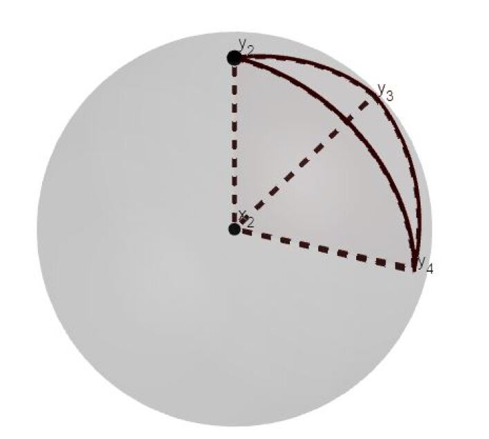
Figure 4. $\wideparen{y_{2}y_{4}}$, $\wideparen{y_{2}y_{3}}$, $\wideparen{y_{3}y_{4}}$ satisfy the triangle inequality

Remark 3.6.

Let us briefly explain why the three angles $\theta$, $\theta_{2}$, $\theta_{4}$ satisfy the triangle inequality. Recall that $\theta=\angle(\overrightarrow{x_{2}x},\overrightarrow{x_{2}x_{4}})$, $\theta_{2}=\angle(\overrightarrow{x_{2}x},\overrightarrow{x_{2}x_{3}})$, $\theta_{4}=\angle(\overrightarrow{x_{2}x_{4}},\overrightarrow{x_{2}x_{3}})$ (See Figure 2). These three angles share the same vertex, $x_{2}$. Let us restrict ourselves in the three dimensional space spanned by the vectors $\{\overrightarrow{x_{2}x},\overrightarrow{x_{2}x_{3}},\overrightarrow{x_{2}x_{4}}\}$, and consider the three dimensional unit sphere $S:=\{y:|y-x_{2}|=1\}$. Suppose that the rays $\overrightarrow{x_{2}x}$, $\overrightarrow{x_{2}x_{3}}$, $\overrightarrow{x_{2}x_{4}}$ intersect with $S$ at the points $y_{2}$, $y_{3}$, $y_{4}$ respectively (see Figure 4). Then $\theta$ is just the length of the arc, which we denote by $\wideparen{y_{2}y_{4}}$, that connects the points $y_{2},y_{4}$ using part of a great circle on $S$. Moreover, the length of the arc $\wideparen{y_{2}y_{4}}$ is the smallest among all possible paths on $S$ that connects $y_{2}$ and $y_{4}$. Thus, the three arcs $\wideparen{y_{2}y_{4}}$, $\wideparen{y_{2}y_{3}}$, $\wideparen{y_{3}y_{4}}$ satisfy the triangle inequality, which is what we desire.

Then we have the following perturbation argument for $C^{1,\beta}$ submanifold without boundary with codimension $k\geq 2$.

Proposition 3.7.

Suppose $r_{2}>0$ is given as the same one in Lemma 3.5. Then for any $p\in(0,\alpha)$, there exists $A_{3}=A_{3}(p,r_{2})>0$ such that for all $x\in D_{\Sigma}$ with $|x|<r_{2}$, we have

$$\bigg{|}p.v.\ \mathcal{A}(d,-\alpha)\int_{D_{\Sigma}}\frac{h(y)^{p}-h(x)^{p}}{|y-x|^{d+\alpha}}dy-C(k,p)h(x)^{p}\delta_{\Sigma}(x)^{-\alpha}\bigg{|}\leq A_{3}(1+\delta_{\Sigma}(x)^{p-\alpha+\beta}+|\log(\delta_{\Sigma}(x))|).$$ (66)

Proof.

Given $x\in D_{\Sigma}$ with $|x|<r_{2}$, the functions $h(x)$ and $h_{x}^{*}$ were already defined as the vertical distance and the distance to the tangent space at $x_{0}$. Recall from (48) that

$$h(x)=\sqrt{1+|\nabla\overrightarrow{\Gamma_{\Sigma}}(\widetilde{x})|^{2}}h_{x}^{*}(x).$$

Then by the calculation of special hyperplane Proposition 2.6, we have

$$p.v.\ \mathcal{A}(d,-\alpha)\int_{D_{\Sigma}}\frac{h_{x}^{*}(y)^{p}-h_{x}^{*}(x)^{p}}{|y-x|^{d+\alpha}}dy-C(k,p)h_{x}^{*}(x)^{p-\alpha}=0.$$

Similar to before, we define $\overrightarrow{\Gamma^{*}}:\mathbb{R}^{d-k}\to\mathbb{R}^{k}$ as the function representing the tangent space at $x_{0}$, i.e.,

$$\Pi_{x}=\{(\widetilde{y},y^{\prime})\in\mathbb{R}^{d-k}\times\mathbb{R}^{k}:y^{\prime}=\overrightarrow{\Gamma^{*}}(\widetilde{y})\}.$$

Denote $D_{\Sigma}^{*}=\mathbb{R}^{d}\backslash\Pi_{x}$, the above two equations lead to

$$p.v.\ \mathcal{A}(d,-\alpha)\int_{D_{\Sigma}}\frac{h(y)^{p}-h(x)^{p}}{|y-x|^{d+\alpha}}dy-C(k,p)h(x)^{p}\delta_{D_{\Gamma}}(x)^{-\alpha}$$

$$=\mathcal{A}(d,-\alpha)\big{(}p.v.\ \int_{D_{\Sigma}}\frac{h(y)^{p}-h(x)^{p}}{|y-x|^{d+\alpha}}dy-p.v.\ \int_{D_{\Sigma}^{*}}\frac{(h_{x}^{*}(y)\sqrt{1+|\nabla\overrightarrow{\Gamma_{\Sigma}}(\widetilde{x})|^{2}})^{p}-h(x)^{p}}{|y-x|^{d+\alpha}}dy\big{)}$$

$$+C(k,p)h(x)^{p}(h_{x}^{*}(x)^{-\alpha}-\delta_{D_{\Sigma}}(x)^{-\alpha})$$

$$:=I+II.$$

For the estimate of $I$, note that the boundary of $D_{\Sigma}$ and $D_{\Sigma}^{*}$ has dimension less than $d-1$, which implies $|\partial D_{\Sigma}|=|\partial D_{\Sigma}^{*}|=0$. Thus

$$I =\mathcal{A}(d,-\alpha)\big{(}p.v.\ \int_{D_{\Sigma}}\frac{h(y)^{p}-h(x)^{p}}{|y-x|^{d+\alpha}}dy-p.v.\ \int_{D_{\Sigma}^{*}}\frac{(h_{x}^{*}(y)\sqrt{1+|\nabla\overrightarrow{\Gamma_{\Sigma}}(\widetilde{x})|^{2}})^{p}-h(x)^{p}}{|y-x|^{d+\alpha}}dy\big{)}$$

$$=\mathcal{A}(d,-\alpha)p.v.\ \int_{\mathbb{R}^{d}}\frac{h(y)^{p}-(h_{x}^{*}(y)\sqrt{1+|\nabla\overrightarrow{\Gamma_{\Sigma}}(\widetilde{x})|^{2}})^{p}}{|y-x|^{d+\alpha}}dy.$$

Now we choose $c_{1}>0$ such that $B(x,r_{2})\subseteq U_{1}$, where $U_{1}$ is define by

$$U_{1}:=\{y=(\widetilde{y},y^{\prime})\in\mathbb{R}^{d-k}\times\mathbb{R}^{k}:|\widetilde{y}-\widetilde{x}|<r_{2},|y^{\prime}|<c_{1}\}.$$ (67)

Then the estimate of $I$ can be splitted into two parts:

$$\frac{1}{\mathcal{A}(d,-\alpha)}|I| \leq\int_{U_{1}}\frac{\big{|}h(y)^{p}-(h_{x}^{*}(y)\sqrt{1+|\nabla\overrightarrow{\Gamma_{\Sigma}}(\widetilde{x})|^{2}})^{p}\big{|}}{|y-x|^{d+\alpha}}dy$$

$$+\int_{B(x,r_{2})^{c}}\frac{\big{|}h(y)^{p}-(h_{x}^{*}(y)\sqrt{1+|\nabla\overrightarrow{\Gamma_{\Sigma}}(\widetilde{x})|^{2}})^{p}\big{|}}{|y-x|^{d+\alpha}}dy.$$

It is easy to see that the second part can be bounded by a universal constant. We only need to focus on the first part. Applying the elementary inequality $|a^{p}-b^{p}|\leq a^{p-1}|a-b|$, we have

$$\big{|}h(y)^{p}-(h_{x}^{*}(y)\sqrt{1+|\nabla\overrightarrow{\Gamma_{\Sigma}}(\widetilde{x})|^{2}})^{p}\big{|}\leq(h_{x}^{*}(y)\sqrt{1+|\nabla\overrightarrow{\Gamma_{\Sigma}}(\widetilde{x})|^{2}})^{p-1}\big{|}h(y)-h_{x}^{*}(y)\sqrt{1+|\nabla\overrightarrow{\Gamma_{\Sigma}}(\widetilde{x})|^{2}}\big{|}$$

Note that $h_{x}^{*}(y)\sqrt{1+|\nabla\overrightarrow{\Gamma_{\Sigma}}(\widetilde{x})|^{2}}$ is actually the vertical distance of $y$ to $\overrightarrow{\Gamma^{*}}$, i.e.,

$$h_{x}^{*}(y)\sqrt{1+|\nabla\overrightarrow{\Gamma_{\Sigma}}(\widetilde{x})|^{2}}=|y^{\prime}-\overrightarrow{\Gamma^{*}}(\widetilde{y})|.$$

Then by triangle inequality, we have

$$\big{|}h(y)-h_{x}^{*}(y)\sqrt{1+|\nabla\overrightarrow{\Gamma_{\Sigma}}(\widetilde{x})|^{2}}\big{|} \leq|\overrightarrow{\Gamma_{\Sigma}}(\widetilde{y})-\overrightarrow{\Gamma^{*}}(\widetilde{y})|=|\overrightarrow{\Gamma_{\Sigma}}(\widetilde{y})-\overrightarrow{\Gamma_{\Sigma}}(\widetilde{x})-(\overrightarrow{\Gamma^{*}}(\widetilde{y})-\overrightarrow{\Gamma^{*}}(\widetilde{x}))|$$

$$\leq c_{2}|\widetilde{y}-\widetilde{x}|^{1+\beta}.$$

For the last inequality, we used the Taylor expansion of $\overrightarrow{\Gamma_{\Sigma}},\overrightarrow{\Gamma^{*}}$ up to order $1+\beta$ and the fact that they are $C^{1,\beta}$ functions. Then our aim is to estimate the following integral:

$$\int_{U_{1}}\frac{\big{|}h(y)^{p}-(h_{x}^{*}(y)\sqrt{1+|\nabla\overrightarrow{\Gamma_{\Sigma}}(\widetilde{x})|^{2}})^{p}\big{|}}{|y-x|^{d+\alpha}}dy\leq\int_{U_{1}}\frac{|y^{\prime}-\overrightarrow{\Gamma^{*}}(\widetilde{y})|^{p-1}|\widetilde{y}-\widetilde{x}|^{1+\beta}}{|y-x|^{d+\alpha}}dy$$

To simplify it, we need to use the following the change of variable

$$\Phi:(\widetilde{y},y^{\prime})\mapsto(\widetilde{y},y^{\prime}-\overrightarrow{\Gamma^{*}}(\widetilde{y})).$$

Note that

$$\Phi(U_{1})\subseteq\{y:|\widetilde{y}-\widetilde{x}|<r_{2},|y^{\prime}|<\widetilde{c_{1}}\}=:\widetilde{U_{1}},$$

and $\Phi$ is Lipschitz: $|\Phi(x)-\Phi(y)|\lesssim|x-y|$, we have

$$\int_{U_{1}}\frac{|y^{\prime}-\overrightarrow{\Gamma^{*}}(\widetilde{y})|^{p-1}|\widetilde{y}-\widetilde{x}|^{1+\beta}}{|y-x|^{d+\alpha}}dy$$

$$\leq c_{2}\int_{U_{1}}\frac{|y^{\prime}-\overrightarrow{\Gamma^{*}}(\widetilde{y})|^{p-1}|\widetilde{y}-\widetilde{x}|^{1+\beta}}{|\Phi(y)-\Phi(x)|^{d+\alpha}}dy$$

$$\leq c_{2}\int_{\widetilde{U}_{1}}\frac{|z^{\prime}|^{p-1}|\widetilde{z}-\widetilde{x}|^{1+\beta}}{\big{(}|\widetilde{z}-\widetilde{x}|^{2}+|z^{\prime}-(x^{\prime}-\overrightarrow{\Gamma^{*}}(\widetilde{x}))|^{2}\big{)}^{(d+\alpha)/2}}dz$$

$$=c_{2}\int_{0}^{r_{2}}\int_{|\widetilde{z}-\widetilde{x}|=r,|z^{\prime}-(x^{\prime}-\overrightarrow{\Gamma^{*}}(\widetilde{x}))|\geq r,\widetilde{U}_{1}}\frac{|z^{\prime}|^{p-1}r^{1+\beta}}{|z^{\prime}-(x^{\prime}-\overrightarrow{\Gamma^{*}}(\widetilde{x}))|^{d+\alpha}}dzdr$$

$$+c_{2}\int_{0}^{r_{2}}\int_{|\widetilde{z}-\widetilde{x}|=r,|z^{\prime}-(x^{\prime}-\overrightarrow{\Gamma^{*}}(\widetilde{x}))|\leq r,\widetilde{U}_{1}}r^{1+\beta-d-\alpha}|z^{\prime}|^{p-1}dzdr$$

$$\leq c_{3}\int_{0}^{r_{2}}\int_{|z^{\prime}|\leq\widetilde{c}_{1},|z^{\prime}-(x^{\prime}-\overrightarrow{\Gamma^{*}}(\widetilde{x}))|\geq r}\frac{|z^{\prime}|^{p-1}r^{d+\beta-k}}{|z^{\prime}-(x^{\prime}-\overrightarrow{\Gamma^{*}}(\widetilde{x}))|^{d+\alpha}}dz^{\prime}dr$$

$$+c_{3}\int_{0}^{r_{2}}\int_{|z^{\prime}|\leq\widetilde{c}_{1},|z^{\prime}-(x^{\prime}-\overrightarrow{\Gamma^{*}}(\widetilde{x}))|\leq r}r^{\beta-\alpha-k}|z^{\prime}|^{p-1}dz^{\prime}dr$$

$$=:c_{3}(I_{1}+I_{2}).$$

For the second inequality, we used the change of variable $z=\Phi(y)$ and for the last inequality, we used the fact that

$$\int_{|\widetilde{z}-\widetilde{x}|=r}d\widetilde{z}\asymp r^{d-k-1}.$$

We split $I_{1}$ into three parts:

$$I_{1} =\bigg{(}\int_{0}^{h(x)/2}+\int_{h(x)/2}^{3h(x)/2}+\int_{3h(x)/2}^{r_{2}}\bigg{)}\int_{|z^{\prime}|\leq\widetilde{c}_{1},|z^{\prime}-(x^{\prime}-\overrightarrow{\Gamma^{*}}(\widetilde{x}))|\geq r}\frac{|z^{\prime}|^{p-1}r^{d+\beta-k}}{|z^{\prime}-(x^{\prime}-\overrightarrow{\Gamma^{*}}(\widetilde{x}))|^{d+\alpha}}dz^{\prime}dr$$

$$=\bigg{(}\int_{0}^{h(x)/2}+\int_{h(x)/2}^{3h(x)/2}+\int_{3h(x)/2}^{r_{2}}\bigg{)}\int_{|z^{\prime}|\leq\frac{\widetilde{c}_{1}}{h(x)},|z^{\prime}-\textbf{e}|\geq\frac{r}{h(x)}}\frac{|z^{\prime}|^{p-1}r^{d+\beta-k}h(x)^{p+k-1-d-\alpha}}{|z^{\prime}-\textbf{e}|^{d+\alpha}}dz^{\prime}dr,$$

Note that $h(x)=|x^{\prime}-\overrightarrow{\Gamma_{\Sigma}}(\widetilde{x})|=|x^{\prime}-\overrightarrow{\Gamma^{*}}(\widetilde{x})|$ because $\overrightarrow{\Gamma_{\Sigma}}(\widetilde{x})=\overrightarrow{\Gamma^{*}}(\widetilde{x})$ and for the second equality, we used the change of variable $\widehat{z}^{\prime}=\frac{z^{\prime}}{h(x)}$ and we denote

$$\textbf{e}=\frac{x^{\prime}-\overrightarrow{\Gamma^{*}}(\widetilde{x})}{|x^{\prime}-\overrightarrow{\Gamma^{*}}(\widetilde{x})|}.$$

We need to estimate them separately.
Estimate of the first term:

$$\int_{0}^{h(x)/2}\int_{|z^{\prime}|\leq\frac{\widetilde{c}_{1}}{h(x)},|z^{\prime}-\textbf{e}|\geq\frac{r}{h(x)}}\frac{|z^{\prime}|^{p-1}r^{d+\beta-k}h(x)^{p+k-1-d-\alpha}}{|z^{\prime}-\textbf{e}|^{d+\alpha}}dz^{\prime}dr$$

$$\leq\int_{0}^{h(x)/2}r^{d+\beta-k}h(x)^{p+k-1-d-\alpha}\bigg{[}\int_{\frac{r}{h(x)}\leq|z^{\prime}-\textbf{e}|\leq\frac{1}{2}}\frac{|z^{\prime}|^{p-1}}{|z^{\prime}-\textbf{e}|^{d+\alpha}}dz^{\prime}+\int_{|z^{\prime}-\textbf{e}|\geq\frac{1}{2}}\frac{|z^{\prime}|^{p-1}}{|z^{\prime}-\textbf{e}|^{d+\alpha}}dz^{\prime}\bigg{]}dr$$

$$\leq c_{4}\int_{0}^{h(x)/2}r^{d+\beta-k}h(x)^{p+k-1-d-\alpha}\bigg{[}\int_{\frac{r}{h(x)}\leq s\leq\frac{1}{2}}\frac{s^{k-1}}{s^{d+\alpha}}ds+1\bigg{]}dr$$

$$\leq c_{5}\int_{0}^{h(x)/2}r^{d+\beta-k}h(x)^{p+k-1-d-\alpha}\bigg{[}(\frac{r}{h(x)})^{k-d-\alpha}+1\bigg{]}dr$$

$$=c_{5}\int_{0}^{h(x)/2}r^{\beta-\alpha}h(x)^{p-1}dr+c_{5}\int_{0}^{h(x)/2}r^{d+\beta-k}h(x)^{p+k-1-d-\alpha}dr$$

$$\leq c_{6}h(x)^{p-\alpha+\beta}$$

For the first inequality, we used the fact that

$$\int_{|z^{\prime}-\textbf{e}|\geq\frac{1}{2}}\frac{|z^{\prime}|^{p-1}}{|z^{\prime}-\textbf{e}|^{d+\alpha}}dz^{\prime}$$

is bounded by a universal constant; for the second inequality above, we used the sphere coordinate and for the last inequality, we used the fact that $\beta>(\alpha-1)_{+}$.
Estimate of the second term:

$$\int_{h(x)/2}^{3h(x)/2}\int_{|z^{\prime}|\leq\frac{\widetilde{c}_{1}}{h(x)},|z^{\prime}-\textbf{e}|\geq\frac{r}{h(x)}}\frac{|z^{\prime}|^{p-1}r^{d+\beta-k}h(x)^{p+k-1-d-\alpha}}{|z^{\prime}-\textbf{e}|^{d+\alpha}}dz^{\prime}dr$$

$$\leq\int_{h(x)/2}^{3h(x)/2}r^{d+\beta-k}h(x)^{p+k-1-d-\alpha}\int_{|z^{\prime}-\textbf{e}|\geq\frac{1}{2}}\frac{|z^{\prime}|^{p-1}}{|z^{\prime}-\textbf{e}|^{d+\alpha}}dz^{\prime}dr$$

$$\leq c_{7}h(x)^{p-\alpha+\beta}.$$

For the first inequality above, we used the fact that

$$\int_{h(x)/2}^{3h(x)/2}r^{d+\beta-k}\asymp h(x)^{d+\beta-k+1}.$$

Estimate of the third term:

$$\int_{3h(x)/2}^{r_{2}}\int_{|z^{\prime}|\leq\frac{\widetilde{c}_{1}}{h(x)},|z^{\prime}-\textbf{e}|\geq\frac{r}{h(x)}}\frac{|z^{\prime}|^{p-1}r^{d+\beta-k}h(x)^{p+k-1-d-\alpha}}{|z^{\prime}-\textbf{e}|^{d+\alpha}}dz^{\prime}dr$$

$$\leq c_{8}\int_{3h(x)/2}^{r_{2}}r^{d+\beta-k}h(x)^{p+k-1-d-\alpha}\int_{|z^{\prime}|\geq\frac{r}{h(x)}}|z^{\prime}|^{p-1-d-\alpha}dz^{\prime}dr$$

$$\leq c_{9}\int_{3h(x)/2}^{r_{2}}r^{d+\beta-k}h(x)^{p+k-1-d-\alpha}(\frac{r}{h(x)})^{p-d-\alpha}dr$$

$$=c_{9}\int_{3h(x)/2}^{r_{2}}r^{p-\alpha+\beta-k}h(x)^{k-1}dr\leq c_{10}h(x)^{p-\alpha+\beta}.$$

For the first inequality, note that when $r\geq\frac{3h(x)}{2}$, $|z^{\prime}-\textbf{e}|\geq\frac{r}{h(x)}$ implies $|z^{\prime}-\textbf{e}|\geq\frac{3}{2}$, thus $|z^{\prime}|\asymp|z^{\prime}-\textbf{e}|$. For the last inequality, note that $k\geq 2$ implies $p-\alpha+\beta-k<-1$, thus

$$\int_{3h(x)/2}^{r_{2}}r^{p-\alpha+\beta-k}dr\lesssim h(x)^{p-\alpha+\beta-k+1}.$$

In summary, combing the estimates of the three terms separately, we get the conclusion that

$$I_{1}\lesssim h(x)^{p-\alpha+\beta}.$$ (68)

To provide the estimate of $I_{2}$, we apply the same procedure as the estimate of $I_{1}$:

$$I_{2} =\int_{0}^{r_{2}}\int_{|z^{\prime}|\leq\widetilde{c}_{1},|z^{\prime}-(x^{\prime}-\overrightarrow{\Gamma^{*}}(\widetilde{x}))|\leq r}r^{\beta-\alpha-k}|z^{\prime}|^{p-1}dz^{\prime}dr$$

$$=\bigg{(}\int_{0}^{h(x)/2}+\int_{h(x)/2}^{3h(x)/2}+\int_{3h(x)/2}^{r_{2}}\bigg{)}r^{\beta-\alpha-k}h(x)^{p+k-1}\int_{|z^{\prime}|\leq\frac{\widetilde{c}_{1}}{h(x)},|z^{\prime}-\textbf{e}|\leq\frac{r}{h(x)}}|z^{\prime}|^{p-1}dz^{\prime}$$

For the second equality, we used the same change of variable and recall that $\textbf{e}=\frac{x^{\prime}-\overrightarrow{\Gamma^{*}}(\widetilde{x})}{|x^{\prime}-\overrightarrow{\Gamma^{*}}(\widetilde{x})|}.$ We will estimate them separately.
Estimate of the first term:

$$\int_{0}^{h(x)/2}r^{\beta-\alpha-k}h(x)^{p+k-1}\int_{|z^{\prime}|\leq\frac{\widetilde{c}_{1}}{h(x)},|z^{\prime}-\textbf{e}|\leq\frac{r}{h(x)}}|z^{\prime}|^{p-1}dz^{\prime}dr$$

$$\leq c_{11}\int_{0}^{h(x)/2}r^{\beta-\alpha-k}h(x)^{p+k-1}\int_{|z^{\prime}-\textbf{e}|\leq\frac{r}{h(x)}}dz^{\prime}dr$$

$$\leq c_{12}\int_{0}^{h(x)/2}r^{\beta-\alpha}h(x)^{p-1}dr=c_{13}h(x)^{p-\alpha+\beta}.$$

For the first inequality, we used the fact that when $r\leq\frac{h(x)}{2}$, $|z^{\prime}-\textbf{e}|\leq\frac{r}{h(x)}$ implies $\frac{1}{2}\leq|z^{\prime}|\leq\frac{3}{2}$; for the second inequality, we used the fact that $\beta>(\alpha-1)_{+}$.
Estimate of the second term:

$$\int_{h(x)/2}^{3h(x)/2}r^{\beta-\alpha-k}h(x)^{p+k-1}\int_{|z^{\prime}|\leq\frac{\widetilde{c}_{1}}{h(x)},|z^{\prime}-\textbf{e}|\leq\frac{r}{h(x)}}|z^{\prime}|^{p-1}dz^{\prime}dr$$

$$\leq\int_{h(x)/2}^{3h(x)/2}r^{\beta-\alpha-k}h(x)^{p+k-1}\int_{|z^{\prime}-\textbf{e}|\leq\frac{3}{2}}|z^{\prime}|^{p-1}dz^{\prime}dr\leq c_{14}h(x)^{p-\alpha+\beta}.$$

Estimate of the third term:

$$\int_{3h(x)/2}^{r_{2}}r^{\beta-\alpha-k}h(x)^{p+k-1}\int_{|z^{\prime}|\leq\frac{\widetilde{c}_{1}}{h(x)},|z^{\prime}-\textbf{e}|\leq\frac{r}{h(x)}}|z^{\prime}|^{p-1}dz^{\prime}dr$$

$$\leq\int_{3h(x)/2}^{r_{2}}r^{\beta-\alpha-k}h(x)^{p+k-1}\bigg{[}\int_{|z^{\prime}-\textbf{e}|\leq\frac{3}{2}}|z^{\prime}|^{p-1}dz^{\prime}+\int_{\frac{3}{2}\leq|z^{\prime}-\textbf{e}|\leq\frac{r}{h(x)}}|z^{\prime}-\textbf{e}|^{p-1}dz^{\prime}\bigg{]}dr$$

$$\leq c_{15}\int_{3h(x)/2}^{r_{2}}r^{\beta-\alpha-k}h(x)^{p+k-1}\bigg{[}1+\int_{\frac{3}{2}\leq s\leq\frac{r}{h(x)}}s^{p+k-2}ds\bigg{]}dr$$

$$\leq c_{16}h(x)^{p-\alpha+\beta}+c_{16}\int_{3h(x)/2}^{r_{2}}r^{p-\alpha-\beta-1}dr$$

$$\leq c_{17}(1+h(x)^{p-\alpha+\beta}+|\log h(x)|)$$

For the second inequality, we used sphere coordinate; for the last inequality, we calculated the integral for $p-\alpha+\beta>0,<0,=0$ separately, same as before.
In summary, the estimate of $I_{2}$ is given as follows:

$$I_{2}\lesssim 1+h(x)^{p-\alpha+\beta}+|\log h(x)|.$$ (69)

For the estimate of $II$, we use Lemma 3.5. In fact,

$$|h(x)^{p}(h_{x}^{*}(x)^{-\alpha}-\delta_{D_{\Sigma}}(x)^{-\alpha})|$$

$$=h(x)^{p}\xi^{-\alpha+1}|h_{x}^{*}(x)-\delta_{D_{\Sigma}}(x)|$$

$$\lesssim\delta_{D_{\Sigma}}(x)^{p}\delta_{D_{\Sigma}}(x)^{-\alpha-1}\delta_{D_{\Sigma}}(x)^{1+\beta}=\delta_{D_{\Sigma}}(x)^{p-\alpha+\beta}.$$

For the first equality, we used mean value theorem for $f(x)=x^{-\alpha}$ and $\xi$ is between $h_{x}^{*}(x)$ and $\delta_{D_{\Sigma}}(x)$. And for the inequality, we have for $|x|<r_{2}$, $|h_{x}^{*}(x)-\delta_{D_{\Sigma}}(x)|\lesssim\delta_{D_{\Sigma}}(x)^{1+\beta}$ by Lemma 3.5. Combing the estimates of $I,II$, we finish the conclusion. ∎

3.3. Perturbation argument for $C^{1,\beta}$ submanifold with codimension $d$.

When $k=d$, $\Sigma_{d,j}$ degenerates to a single point and this case is easier and essentially covered in [6]. In fact, without loss of generality, we assume our open set is $D=\mathbb{R}^{d}\backslash\{0\}$. In this case, the vertical distance $h(x)$ is the same as the distance:

$$h(x):=|x|=\delta_{D}(x).$$

Our perturbation argument in this case is given by Proposition 2.6.

3.4. Perturbation argument for the general case

The assumption on the open set $D$ allows us to write $D$ as

$$D=D^{\prime}\backslash\bigcup_{k=2}^{d}\bigcup_{j=1}^{m_{k}}\Sigma_{k,j},$$

where $D^{\prime}$ is a $C^{1,\beta}$ open set such that $\bigcup_{k=2}^{d}\bigcup_{j=1}^{m_{k}}\Sigma_{k,j}\subseteq D^{\prime}$ and $\partial D^{\prime}=\cup_{j=1}^{m_{1}}\Gamma_{1.j}$. Also recall that for each $1\leq j\leq m_{d}$, $\Gamma_{d,j}$ is a single point. It is easy to see that $\{\Gamma_{k,j}\}_{1\leq k\leq d,1\leq j\leq m_{k}}$ are disjoint, thus we can define

$$s_{1}:=\min\{d(\Sigma_{k,j},\Sigma_{k^{\prime},j^{\prime}}):1\leq k,k^{\prime}\leq d,1\leq j\leq m_{k},1\leq j^{\prime}\leq m_{k^{\prime}},(k,j)\neq(k^{\prime},j^{\prime})\}>0,$$

which is ensured by the disjointness of $\{\Sigma_{k,j}\}_{1\leq k\leq d,1\leq j\leq m_{k}}$. Moreover, suppose $(R_{k,j},\Lambda_{k,j})$ are the characteristics of $\Sigma_{k,j}$, denote

$$s_{2}:=\min\{R_{k,j}:1\leq k\leq d,1\leq j\leq m_{k}\}>0$$

and

$$\Lambda:=\max\{\Lambda_{k,j}:1\leq k\leq d,1\leq j\leq m_{k}\}.$$ (70)

Since the definition of vertical distance requires us to choose a local coordinate system and the underlying function, the local coordinate system should be specified for perturbation argument.
Given any point $w\in\partial D$, we can assume $w\in\Gamma_{k,j}$ for some $1\leq k\leq d,1\leq j\leq m_{j}$, then (27), (28) or (29) holds according to the value of $k$. We can define our vertical distance function $h_{w}$ by

$$h_{w}(y):=\begin{cases}|y_{d}-\Gamma(\widetilde{y})|1_{B(w,\frac{s_{1}\wedge s_{2}}{2})\cap D}(y),\ k=1\\ |y^{\prime}-\overrightarrow{\Gamma}(\widetilde{y})|1_{B(w,\frac{s_{1}\wedge s_{2}}{2})\cap D}(y),\ k=2,\cdots,d-1\\ |y-w|1_{B(w,\frac{s_{1}\wedge s_{2}}{2})\cap D}(y),k=d.\end{cases}$$ (71)

The following perturbation argument for the general case follows from the perturbation arguments of $C^{1,\beta}$ open set and $C^{1,\beta}$ submanifold without boundary with codimension $k\geq 2$ separately:

Proposition 3.8.

There exists a universal constant $0<R<\frac{s_{1}}{2}\wedge\frac{s_{2}}{2}\wedge\frac{1}{2}$, such that for any

$$p\in[\alpha-1,a)\cap(0,\alpha),\ k=1$$

$$p\in(0,\alpha),k\geq 2,$$

there exists $A_{4}>0,\gamma>0$ independent of $w$, such that for all $x\in B(w,R)\cap D$ we have

$$\bigg{|}p.v.\ \mathcal{A}(d,-\alpha)\int_{D}\frac{h_{w}(y)^{p}-h_{w}(x)^{p}}{|y-x|^{d+\alpha}}dy-C(k,p)h_{w}(x)^{p}\delta_{D}(x)^{-\alpha}\bigg{|}$$ (72)

$$\leq A_{4}(1+\delta_{D}(x)^{p-\alpha+\gamma}+|\log(\delta_{D}(x))|).$$

Proof.

First we define the untruncated vertical distance $\bar{h}_{w}$ by :

$$\bar{h}_{w}(y):=\begin{cases}|y_{d}-\Gamma(\widetilde{y})|,\ k=1\\ |y^{\prime}-\overrightarrow{\Gamma}(\widetilde{y})|,\ k=2,\cdots,d-1\\ |y-w|,k=d.\end{cases}$$ (73)

Case 1: k=1: Then by Proposition 3.4, we have for any $x\in B(w,r_{1})\cap D_{\Gamma}$

$$\bigg{|}p.v.\ \mathcal{A}(d,-\alpha)\int_{D_{\Gamma}}\frac{\bar{h}_{w}(y)^{p}-\bar{h}_{w}(x)^{p}}{|y-x|^{d+\alpha}}dy-C(k,p)\bar{h}_{w}(x)^{p}\delta_{D}(x)^{-\alpha}\bigg{|}$$

$$\leq A_{1}(1+\delta_{D}(x)^{p-\alpha+\gamma}+|\log(\delta_{D}(x))|).$$

Note that if we further assume that $x\in B(w,\frac{s_{1}\wedge s_{2}}{2})\cap D$, $\bar{h}_{w}(x)=h_{w}(x)$. Also note that

$$B(w,s_{1}\wedge s_{2})\cap D=B(w,s_{1}\wedge s_{2})\cap D_{\Gamma}.$$

Define

$$R:=\frac{s_{1}\wedge s_{2}\wedge r_{1}\wedge r_{2}}{4}.$$

For $x\in B(w,R)\cap D$,

$$\bigg{|}p.v.\ \mathcal{A}(d,-\alpha)\int_{D}\frac{h_{w}(y)^{p}-h_{w}(x)^{p}}{|y-x|^{d+\alpha}}dy-C(1,p)h_{w}(x)^{p}\delta_{D}(x)^{-\alpha}\bigg{|}$$

$$\leq\bigg{|}p.v.\ \mathcal{A}(d,-\alpha)\int_{D_{\Gamma}}\frac{\bar{h}_{w}(y)^{p}-\bar{h}_{w}(x)^{p}}{|y-x|^{d+\alpha}}dy-C(k,p)\bar{h}_{w}(x)^{p}\delta_{D}(x)^{-\alpha}\bigg{|}$$

$$+\mathcal{A}(d,-\alpha)\bigg{(}\int_{B(w,\frac{s_{1}\wedge s_{2}\wedge r_{1}}{2})^{c}\cap D_{\Gamma}}\frac{|\bar{h}_{w}(y)^{p}-\bar{h}_{w}(x)^{p}|}{|y-x|^{d+\alpha}}dy+\int_{B(w,\frac{s_{1}\wedge s_{2}\wedge r_{1}}{2})^{c}\cap D}\frac{|\bar{h}_{w}(y)^{p}-\bar{h}_{w}(x)^{p}|}{|y-x|^{d+\alpha}}dy\bigg{)}$$

$$\lesssim 1+\delta_{D}(x)^{p-\alpha+\gamma}+|\log(\delta_{D}(x))|.$$

Case 2: $2\leq k\leq d-1$ if $d>2$: This case follows from the same argument except that we use $D_{\overrightarrow{\Gamma}}$ instead of $D_{\Gamma}$ and Proposition 3.7.
Case 3: $k=d$: Assume $\Gamma_{d,j}=\{0\}$. This case follows from the same argument except that we use $\mathbb{R}^{d}\backslash\{0\}$ instead of $D_{\Gamma}$ and Proposition 2.6. ∎

4. Proof of the main theorem

In this section we consider the following operators with multi-singular killing potentials:

$$\mathcal{L}^{\kappa}f(x):=-(-\Delta|_{D})^{\frac{\alpha}{2}}f(x)+\kappa(x)f(x)$$ (74)

where $\kappa(x)=-\sum_{k=1}^{d}\sum_{j=1}^{m_{k}}\lambda_{k,j}\delta_{\Sigma_{k,j}}(x)^{-\alpha},\lambda_{k,j}>0$.
From the factorization result of heat kernels, we only need to show: For fixed $T>0$, for any $t\in(0,T)$, $x\in D$ we have

$$\mathbb{P}^{x}(\tau_{D}>t)\asymp\prod_{k=1}^{d}\prod_{j=1}^{m_{k}}(1\wedge\frac{\delta_{\Gamma_{k,j}}(x)}{t^{1/\alpha}})^{p_{k,j}},$$

where $C(k,p_{k,j})=\lambda_{k,j}$ through (19) or (20) for $k=1$ or $k\geq 2$. From now on $x,t$ will be fixed.
Suppose $\delta_{D}(x)=\delta_{\Gamma_{k,j}}(x)$ for some $1\leq k\leq d,1\leq j\leq m_{k}$. We have three cases to consider: $k=1$ or $2\leq k\leq d-1$(if $d>2$) or $k=d$.
Case 1: $k=1$. In this case, we choose $x_{0}\in\Gamma_{1,j}$ such that $\delta_{\Gamma_{1,j}}(x)=|x-x_{0}|$. Now we construct a local coordinate system $CS_{x_{0}}$ such that

$$B(x_{0},R)\cap D=\{(\widetilde{y},y_{d}):y_{d}>\Gamma(\widetilde{y})\}\cap B(x_{0},R),$$

where $\Gamma$ is a $C^{1,\beta}$ function such that $\Gamma(x_{0})=0,\nabla\Gamma(x_{0})=0$. Then define

$$h_{x}(y):=|y_{d}-\Gamma(\widetilde{y})|1_{B(x_{0},R)\cap D}(y)$$ (75)

By Proposition 3.8, for any $p\in(0,\alpha)$, there exists $A_{2}>0,\gamma>0$, such that for any $z\in B(x_{0},R)\cap D$,

$$\bigg{|}(\Delta)^{\frac{\alpha}{2}}(h_{x}^{p})(z)-C(1,p)h_{x}(z)^{p}\delta_{D}(z)^{-\alpha}\bigg{|}\leq A_{2}(1+\delta_{D}(z)^{p-\alpha+\gamma}+|\log(\delta_{D}(z))|).$$

Now we are able to construct super(sub)-harmonic function based on the above estimates: choose $q_{1,j}\in(p_{1,j},(p_{1,j}+\gamma)\wedge\alpha)$, define

$$v_{1}(y):=h_{x}^{p_{1,j}}(y)+h_{x}^{q_{1,j}}(y),v_{2}(y):=h_{x}^{p_{1,j}}(y)-h_{x}^{q_{1,j}}(y).$$ (76)

For any constant $s>0$, we denote

$$\mathcal{U}(x,s):=B(x_{0},s)\cap D$$ (77)

Then it is easy to show the following lemma:

Lemma 4.1.

There exists $\widetilde{r}_{3}\in(0,R)$, independent of $x$ and $t$, such that for any $z\in\mathcal{U}(x,\widetilde{r}_{3})$,

$$\mathcal{L}^{\kappa}(v_{1})(z)\gtrsim\delta_{D}(z)^{q_{k,j}-\alpha},$$ (78)

$$\mathcal{L}^{\kappa}(v_{2})(z)\lesssim-\delta_{D}(z)^{q_{k,j}-\alpha},$$

where the implicit constants are independent of $z,x,t$.

Proof.

Recall that $\lambda_{1,j}=C(1,p_{1,j})$ through (19), we have

$$\mathcal{L}^{\kappa}(v_{1})(z)$$

$$=p.v.\ \mathcal{A}(d,-\alpha)\int_{D}\frac{h_{x}(y)^{p_{1,j}}-h_{x}(z)^{p_{1,j}}}{|y-z|^{d+\alpha}}dy-C(1,p_{1,j})h_{x}(z)^{p_{1,j}}\delta_{D}(z)^{-\alpha}$$

$$+p.v.\ \mathcal{A}(d,-\alpha)\int_{D}\frac{h_{x}(y)^{q_{1,j}}-h_{x}(z)^{q_{1,j}}}{|y-z|^{d+\alpha}}dy-C(1,q_{1,j})h_{x}(z)^{q_{1,j}}\delta_{D}(z)^{-\alpha}$$

$$+(C(1,q_{1,j})-C(1,p_{1,j}))h_{x}(z)^{q_{1,j}}\delta_{D}(z)^{-\alpha}-\sum_{(\widetilde{k},\widetilde{j})\neq(1,j)}\lambda_{\widetilde{k},\widetilde{j}}\delta_{\Gamma_{\widetilde{k},\widetilde{j}}}(z)^{-\alpha}v_{1}(z)$$

$$\geq-2A_{2}(1+\delta_{D}(z)^{p_{1,j}-\alpha+\gamma}+|\log(\delta_{D}(z))|+\delta_{D}(z)^{q_{1,j}-\alpha+\gamma})+c_{1}\delta_{D}(z)^{q_{1,j}-\alpha}-c_{2}.$$

For the inequality above, we used Proposition 3.8, $C(1,\cdot)$ is a strictly increasing function thus $(C(1,q_{1,j})-C(1,p_{1,j}))>0$, the fact that $\delta_{\Gamma_{\widetilde{k},\widetilde{j}}}(z)\geq R$ for $z\in\mathcal{U}(x,R)$ thus $\delta_{\Gamma_{\widetilde{k},\widetilde{j}}}(z)^{-\alpha}\leq R^{-\alpha}$ and $h_{x}(z)\asymp\delta_{D}(z)$ for $z\in\mathcal{U}(x,R)$.
Now recall that $q_{1,j}\in(p_{1,j},(p_{1,j}+\gamma)\wedge\alpha)$, we have either $p_{1,j}-\alpha+\gamma>0$ or $q_{1,j}-\alpha<p_{1,j}-\alpha+\gamma$. For both cases, $q_{1,j}-\alpha$ is the smallest negative constant thus $\delta_{D}(z)^{q_{1,j}-\alpha}$ is the dominant term as $\delta_{D}(z)$ goes to zero. In other words, we can choose a constant $\widetilde{r}_{3}\in(0,R)$ such that

$$\mathcal{L}^{\kappa}(v_{1})(z)\gtrsim\delta_{D}(z)^{q_{1,j}-\alpha},z\in\mathcal{U}(x,\widetilde{r}_{3}).$$

Following the same calculations, we can show that

$$\mathcal{L}^{\kappa}(v_{2})(z)\lesssim-\delta_{D}(z)^{q_{1,j}-\alpha},z\in\mathcal{U}(x,\widetilde{r}_{3}).$$

∎

To continue our probabilistic analysis, we need to apply Dynkin’s formula. The problem is that $v_{1},v_{2}$ are not in the domain $\mathcal{D}(\mathcal{L}^{\kappa})$ of $\mathcal{L}^{\kappa}$. In fact, they are not even continuous. However, by a standard mollifying procedure, we can avoid this technical issue.

Lemma 4.2.

There exist uniformly bounded $\{f_{n}\},\{g_{n}\}\in C_{c}^{\infty}\subseteq\mathcal{D}(\mathcal{L}^{\kappa})$, a strictly decreasing positive sequence $a_{n}\to 0$, and $r_{3}\in(0,\widetilde{r}_{3}/2)$ such that

• $\lim_{n\to\infty}f_{n}=v_{1},\ \lim_{n\to\infty}g_{n}=v_{2}$ pointwisely on $\mathcal{U}(x,r_{3})$.

• For sufficiently large $n$, we have $\mathcal{L}^{\kappa}(f_{n})(z)\geq 0$ and $\mathcal{L}^{\kappa}(g_{n})(z)\leq 0$ for any $z\in\mathcal{U}(x,r_{3})$ with $\delta_{D}(z)>a_{n}$.

Due to the technicality of the proof, we put it in the Appendix. Assuming Lemma 4.2, we are able to prove the following:

Theorem 4.3.

$\mathbb{P}^{x}(\tau_{D}>t)\asymp(1\wedge\frac{\delta_{D}(x)}{t^{1/\alpha}})^{p_{1,j}}$, where the implicit constants are independent of $x,t$.

Proof.

First choose $C_{1}:=\frac{r_{3}T^{-\frac{1}{\alpha}}}{4}$ and define

$$r=r_{t}=C_{1}t^{\frac{1}{\alpha}}.$$ (79)

If $\delta_{D}(x)\geq r$, then by the interior estimates Lemma 2.3, we have $\mathbb{P}^{x}(\tau_{D}>t)\asymp 1$. Thus we can assume $\delta_{D}(x)=|x-x_{0}|<r=C_{1}t^{1/\alpha}<r_{3}/4$. For any constant $s>0$, we denote

$$D^{int}(s):=\{y\in D:\delta_{D}(y)>s\}$$ (80)

Recall that $a_{n}$ is the sequence given in Lemma 4.2, we have

$$D^{int}(a_{1})\subset\joinrel\subset\cdots\subset\joinrel\subset D^{int}(a_{n})\to D,$$

then for the following sequence of exit times $\tau_{\mathcal{U}(x,r)\cap D^{int}(a_{n})}:=\{t>0:Y_{t}\notin\mathcal{U}(x,r)\cap D^{int}(a_{n})\}$, we have

$$\lim_{n\to\infty}\tau_{\mathcal{U}(x,r)\cap D^{int}(a_{n})}=\tau_{\mathcal{U}(x,r)},\mathbb{P}-a.s.$$ (81)

Then apply Dynkin’s formula, bounded convergence theorem and quasi-left continuity of $Y_{t}$, we have

$$v_{1}(x)=\lim_{n\to\infty}f_{n}(x) =\lim_{n\to\infty}\bigg{[}\mathbb{E}^{x}\big{(}f_{n}(Y_{\tau_{\mathcal{U}(x,r)\cap D^{int}(a_{n})}})\big{)}-\mathbb{E}^{x}\bigg{(}\int_{0}^{\tau_{\mathcal{U}(x,r)\cap D^{int}(a_{n})}}\mathcal{L}^{\kappa}(f_{n})(Y_{s})ds\bigg{)}\bigg{]}$$

$$\leq\lim_{n\to\infty}\mathbb{E}^{x}\big{(}f_{n}(Y_{\tau_{\mathcal{U}(x,r)\cap D^{int}(a_{n})}})\big{)}=\mathbb{E}^{x}\big{(}v_{1}(Y_{\tau_{\mathcal{U}(x,r)}})\big{)}.$$

Since we choose $r=C_{1}t^{1/\alpha}<r_{3}/4$, we have $\mathcal{U}(x,2r)\subseteq\mathcal{U}(x,r_{3})\subseteq\mathcal{U}(x,R)$. Then

$$E^{x}\big{(}v_{1}(Y_{\tau_{\mathcal{U}(x,r)}})\big{)}$$

$$=E^{x}\big{(}v_{1}(Y_{\tau_{\mathcal{U}(x,r)}});Y_{\tau_{\mathcal{U}(x,r)}}\in\mathcal{U}(x,2r)\big{)}+\sum_{n\geq 1}E^{x}\big{(}v_{1}(Y_{\tau_{\mathcal{U}(x,r)}});Y_{\tau_{\mathcal{U}(x,r)}}\in\mathcal{U}(x,2^{n+1}r)\backslash U(x,2^{n}r)\big{)}.$$

Recall that by Lemma 3.2, we have

$$v_{1}(y)\lesssim h_{x}(y)^{p}\lesssim r^{p},\ y\in\mathcal{U}(x,2r),$$

$$v_{1}(y)\lesssim h_{x}(y)^{p}\lesssim 2^{pn}r^{p},\ y\in\mathcal{U}(x,2^{n+1}r)\backslash U(x,2^{n}r).$$

Then by Lévy system formula, we have

$$\mathbb{P}^{x}(Y_{\tau_{\mathcal{U}(x,r)}}\in\mathcal{U}(x,2r))\gtrsim\mathbb{E}^{x}\int_{0}^{\tau_{\mathcal{U}(x,r)}}\int_{\mathcal{U}(x,2r)}\frac{1}{|Y_{s}-z|^{d+\alpha}}dzds\gtrsim r^{-\alpha}\mathbb{E}^{x}(\tau_{\mathcal{U}(x,r)}).$$ (82)

Moreover, for each $n\geq 1$, we have

$$\mathbb{E}^{x}\big{(}v_{1}(Y_{\tau_{\mathcal{U}(x,r)}});Y_{\tau_{\mathcal{U}(x,r)}}\in\mathcal{U}(x,2^{n+1}r)\backslash U(x,2^{n}r)\big{)}$$

$$\lesssim 2^{nq_{1,j}}r^{p_{1,j}}\mathbb{P}^{x}(Y_{\tau_{\mathcal{U}(x,r)}}\in\mathcal{U}(x,2^{n+1}r)\backslash U(x,2^{n}r))$$

$$\lesssim 2^{nq_{1,j}}r^{p_{1,j}}\mathbb{E}^{x}\int_{0}^{\tau_{\mathcal{U}(x,r)}}\int_{\mathcal{U}(x,2^{n+1}r)\backslash U(x,2^{n}r))}\frac{1}{|Y_{s}-z|^{d+\alpha}}dzds$$

$$\lesssim 2^{n(q_{1,j}-\alpha)}r^{p_{1,j}}r^{-\alpha}\mathbb{E}^{x}(\tau_{\mathcal{U}(x,r)})$$

$$\lesssim 2^{n(q_{1,j}-\alpha)}r^{p_{1,j}}\mathbb{P}^{x}(Y_{\tau_{\mathcal{U}(x,r)}}\in\mathcal{U}(x,2r)),$$

where for the last inequality, we used (82). Thus

$$\mathbb{E}^{x}\big{(}v_{1}(Y_{\tau_{\mathcal{U}(x,r)}})\big{)}$$

$$=\mathbb{E}^{x}\big{(}v_{1}(Y_{\tau_{\mathcal{U}(x,r)}});Y_{\tau_{\mathcal{U}(x,r)}}\in\mathcal{U}(x,2r)\big{)}+\sum_{n\geq 1}\mathbb{E}^{x}\big{(}v_{1}(Y_{\tau_{\mathcal{U}(x,r)}});Y_{\tau_{\mathcal{U}(x,r)}}\in\mathcal{U}(x,2^{n+1}r)\backslash U(x,2^{n}r)\big{)}$$

$$\lesssim r^{p_{1,j}}\mathbb{P}^{x}(Y_{\tau_{\mathcal{U}(x,r)}}\in\mathcal{U}(x,2r))+\sum_{n\geq 1}2^{n(q_{1,j}-\alpha)}r^{p_{1,j}}\mathbb{P}^{x}(Y_{\tau_{\mathcal{U}(x,r)}}\in\mathcal{U}(x,2r))$$

$$\lesssim r^{p_{1,j}}\mathbb{P}^{x}(Y_{\tau_{\mathcal{U}(x,r)}}\in\mathcal{U}(x,2r))\leq r^{p_{1,j}}\mathbb{P}^{x}(Y_{\tau_{\mathcal{U}(x,r)}}\in D).$$

Then by Lemma 2.4, we have

$$\mathbb{P}^{x}(\tau_{D}>t)\asymp\mathbb{P}^{x}(Y_{\tau_{\mathcal{U}(x,r)}}\in D)\gtrsim\frac{v_{1}(x)}{r^{p_{1,j}}}\gtrsim\frac{\delta_{D}(x)^{p_{1,j}}}{t^{1/\alpha}},$$

which finishes the lower bound of the theorem. For the upper bound, by applying a similar Dynkin’s formula argument to $g_{n}$, we have

$$v_{2}(x)\geq\mathbb{E}^{x}(v_{2}(Y_{\tau_{\mathcal{U}(x,r)}})).$$ (83)

Now we choose a ball $\mathcal{B}_{t}:=B(w,ct^{1/\alpha})\subseteq\mathcal{U}(x,R)$ such that

$$\mathcal{B}_{t}\cap\mathcal{U}(x,r)=\emptyset,\text{moreover,}\ {\rm dist}(\mathcal{B}_{t},\mathcal{U}(x,r))\gtrsim r^{1/\alpha},$$

$$\delta_{D}(y)\asymp r,\ \forall y\in\mathcal{B}_{t}$$

Then

$$\delta_{D}(x)^{p_{1,j}} \gtrsim v_{2}(x)\geq\mathbb{E}^{x}(v_{2}(Y_{\tau_{\mathcal{U}(x,r)}}))\geq E^{x}(v_{2}(Y_{\tau_{\mathcal{U}(x,r)}});Y_{\tau_{\mathcal{U}(x,r)}}\in\mathcal{B}_{t})$$

$$\gtrsim(r^{p_{1,j}}-r^{q_{1,j}})\mathbb{P}^{x}(Y_{\tau_{\mathcal{U}(x,r)}}\in\mathcal{B}_{t})\gtrsim r^{p_{1,j}}\mathbb{P}^{x}(Y_{\tau_{\mathcal{U}(x,r)}}\in\mathcal{B}_{t}),$$

where the last inequality follows from $p_{1,j}<q_{1,j}$ and $r$ is very small. Then by Lemma 2.4, we have

$$\mathbb{P}^{x}(\tau_{D}>t)\asymp\mathbb{P}^{x}(Y_{\tau_{\mathcal{U}(x,r)}}\in D)\asymp\mathbb{P}^{x}(Y_{\tau_{\mathcal{U}(x,r)}}\in\mathcal{B}_{t})\lesssim\frac{\delta_{D}(x)^{p_{1,j}}}{t^{1/\alpha}},$$

which concludes the proof. ∎

Now recall that from the assumption of the open set $D$, different components of $\partial D$ are separate from each other with at least distance $2R$. Then if $\delta_{D}(x)=|x-x_{0}|$ where $x_{0}\in\Gamma_{1,j}$, we have

$$\delta_{\Gamma_{\widetilde{k},\widetilde{j}}}(x)\geq R,\ (\widetilde{k},\widetilde{j})\neq(1,j).$$

Therefore, for $(\widetilde{k},\widetilde{j})\neq(1,j)$, we have

$$1\wedge\frac{\delta_{\Gamma_{\widetilde{k},\widetilde{j}}}(x)}{t^{1/\alpha}}\asymp 1,\ \text{if}\ \delta_{D}(x)=\delta_{\Gamma_{1,j}}(x).$$

In summary, we have

$$\mathbb{P}^{x}(\tau_{D}>t)\asymp(1\wedge\frac{\delta_{\Gamma_{1,j}}(x)}{t^{1/\alpha}})^{p_{1,j}}\asymp\prod_{\widetilde{k}=1}^{d}\prod_{\widetilde{j}=1}^{m_{\widetilde{k}}}(1\wedge\frac{\delta_{\Gamma_{\widetilde{k},\widetilde{j}}}(x)}{t^{1/\alpha}})^{p_{\widetilde{k},\widetilde{j}}}.$$

Case 2: $2\leq k\leq d-1$ if $d>2$. In this case, we choose $x_{0}\in\Gamma_{k,j}$ such that $\delta_{\Gamma_{k,j}}(x)=|x-x_{0}|$. Now we construct a local coordinate system $CS_{x_{0}}$ such that

$$B(x_{0},R)\cap D=\{(\widetilde{y},y^{\prime})\in\mathbb{R}^{d-k}\times\mathbb{R}^{k}:y^{\prime}\neq\overrightarrow{\Gamma}(\widetilde{y})\}\cap B(x_{0},R),$$

where $\Gamma$ is a $C^{1,\beta}$ vector-valued function such that $\overrightarrow{\Gamma}(x_{0})=0,\nabla\overrightarrow{\Gamma}(x_{0})=0$. Then define

$$\widetilde{h}_{x}(y):=|y^{\prime}-\Gamma(\widetilde{y})|1_{B(x_{0},R)\cap D}(y)$$ (84)

Then following the same procedure, construct

$$\widetilde{v}_{1}(y):=\widetilde{h}_{x}^{p_{k,j}}(y)+\widetilde{h}_{x}^{q_{k,j}}(y),\widetilde{v}_{2}(y):=\widetilde{h}_{x}^{p_{k,j}}(y)-\widetilde{h}_{x}^{q_{k,j}}(y),$$ (85)

we arrive at the conclusion that

$$\mathbb{P}^{x}(\tau_{D}>t)\asymp(1\wedge\frac{\delta_{\Gamma_{k,j}}(x)}{t^{1/\alpha}})^{p_{k,j}}\asymp\prod_{\widetilde{k}=1}^{d}\prod_{\widetilde{j}=1}^{m_{\widetilde{k}}}(1\wedge\frac{\delta_{\Gamma_{\widetilde{k},\widetilde{j}}}(x)}{t^{1/\alpha}})^{p_{\widetilde{k},\widetilde{j}}}.$$

Case 3: $k=d$. In this case, $\Gamma_{d,j}$ degenerates to a single point $\{x_{0}\}$. Then we construct our testing function as

$$\hat{v}_{1}(y):=|y-x_{0}|^{p_{k,j}}1_{\mathcal{U}(x,R)}(y)+|y-x_{0}|^{q_{k,j}}1_{\mathcal{U}(x,R)}(y),$$ (86)

$$\hat{v}_{2}(y):=|y-x_{0}|^{p_{k,j}}1_{\mathcal{U}(x,R)}(y)-|y-x_{0}|^{q_{k,j}}1_{\mathcal{U}(x,R)}(y).$$

Applying the same procedure, we arrive at the conclusion that

$$\mathbb{P}^{x}(\tau_{D}>t)\asymp(1\wedge\frac{\delta_{\Gamma_{d,j}}(x)}{t^{1/\alpha}})^{p_{d,j}}\asymp\prod_{\widetilde{k}=1}^{d}\prod_{\widetilde{j}=1}^{m_{\widetilde{k}}}(1\wedge\frac{\delta_{\Gamma_{\widetilde{k},\widetilde{j}}}(x)}{t^{1/\alpha}})^{p_{\widetilde{k},\widetilde{j}}}.$$

Thus we finish the whole proof of the main theorem.

5. Appendix

In the appendix, we aim to make up some technical details we owe in the main text.

Proof of Lemma 4.2: First we choose a nonnegative function $\varphi\in C_{c}^{\infty}(\mathbb{R}^{d})$ such that $\text{supp}\ \varphi\subseteq B(0,1)$ and $\int_{\mathbb{R}^{d}}\varphi(u)du=1$. Now we choose three positive sequences $\{a_{n}\},\{b_{n}\},\{c_{n}\}$ tending to zero, which we will specify later. Define

$$\varphi_{n}(y):=c_{n}^{d}\varphi(c_{n}y),f_{n}:=\varphi_{n}*(v_{1}1_{D^{int}(b_{n})}),\ g_{n}:=\varphi_{n}*(v_{2}1_{D^{int}(b_{n})}).$$

Then we claim that for properly chosen $\{a_{n}\},\{b_{n}\},\{c_{n}\}$, there exists a constant $r_{3}\in(0,\widetilde{r}_{3})$ such that for sufficiently large $n$, we have

$$\mathcal{L}^{\kappa}(f_{n})(z)\geq 0,\ \mathcal{L}^{\kappa}(g_{n})(z)\leq 0$$

for any $z\in\mathcal{U}(x,r_{3})\cap D^{int}(a_{n})$. Here we recall that the definitions of $\mathcal{U}(x,r_{3})$ and $D^{int}(a_{n})$ are (77) and (80).

$$\mathcal{L}^{\kappa}(f_{n})(z)=\mathcal{L}^{\kappa}(\varphi_{n}*v_{1})(z)-\mathcal{L}^{\kappa}(\varphi_{n}*v_{1}-f_{n})(z)$$

$$=\mathcal{L}^{\kappa}(\varphi_{n}*v_{1})(z)$$

$$+\mathcal{A}(d,-\alpha)\text{p.v.}\ \int_{D}\int_{\mathbb{R}^{d}}\varphi_{n}(u)\frac{\big{(}1_{D^{int}(b_{n})}(y-u)-1\big{)}v_{1}(y-u)-\big{(}1_{D^{int}(b_{n})}(z-u)-1\big{)}v_{1}(z-u)}{|y-z|^{d+\alpha}}dudy$$

$$+\kappa(z)\int_{\mathbb{R}^{d}}\varphi_{n}(u)\big{(}1_{D^{int}(b_{n})}(z-u)-1\big{)}v_{1}(z-u)du$$

$$=:I+II+III.$$

The main challenge comes from $I$. Since $\text{supp}\ \varphi_{n}\subseteq B(0,c_{n})$, thus under the assumptions that

$$\lim_{n\to\infty}\frac{c_{n}}{a_{n}}=0,\lim_{n\to\infty}\frac{b_{n}}{a_{n}}=0,$$ (87)

we have for sufficiently large $n$, $z-u\in D^{int}(b_{n})$ for any $z\in D^{int}(a_{n})$ and $|u|<c_{n}$ thus

$$1_{D^{int}(b_{n})}(z-u)-1=0.$$

Then it is clear that $III$ is equal to zero. For the estimate of $II$, we have

$$|II| =\mathcal{A}(d,-\alpha)\text{p.v.}\ \int_{D}\int_{\mathbb{R}^{d}}\varphi_{n}(u)\frac{\big{(}1-1_{D^{int}(b_{n})}(y-u)\big{)}v_{1}(y-u)}{|y-z|^{d+\alpha}}dudy$$

$$\lesssim\int_{y\in\mathcal{U}(x,R),\delta_{D}(y)\leq 2b_{n}}\int_{\mathbb{R}^{d}}\varphi_{n}(u)\frac{\delta_{D}(y-u)^{p_{1,j}}}{|y-z|^{d+\alpha}}dudy$$

$$\lesssim b_{n}^{p_{1,j}}\int_{y\in\mathcal{U}(x,R),\delta_{D}(y)\leq 2b_{n}}\frac{1}{|y-z|^{d+\alpha}}dy$$

$$\lesssim b_{n}^{p_{1,j}}(a_{n}-2b_{n})^{-d-\alpha}.$$

For the first inequality above, note that if $\delta_{D}(y)>2b_{n}$, we have $\delta_{D}(y-u)\geq 2b_{n}-c_{n}>b_{n}$ thus $1-1_{D^{int}(b_{n})}(y-u)=0$ and recall that from the definition of $v_{1}$ we have $v_{1}(y)\lesssim\delta_{D}(y)^{p_{1,j}}$ for any $y\in\mathcal{U}(x,R)$. For the second inequality, note that $\delta_{D}(y-u)\leq\delta_{D}(y)+|u|\lesssim b_{n}+c_{n}\lesssim b_{n}$. For the last inequality, we use the fact that if $\delta_{D}(y)\leq 2b_{n}$ and $\delta_{D}(z)>a_{n}$, we have $|y-z|\geq a_{n}-2b_{n}$, which is greater than $0$ for $n$ large under the assumption (87).
In summary, if we assume

$$\lim_{n\to\infty}b_{n}^{p_{1,j}}(a_{n}-2b_{n})^{-d-\alpha}=0,$$ (88)

$|II|$ is small for large $n$, which will be enough to conclude our result.
Now we turn to the estimate of $I$:

$$I =\text{p.v.}\int_{D}\int_{\mathbb{R}^{d}}\varphi_{n}(u)\frac{v_{1}(y-u)-v_{1}(z-u)}{|y-z|^{d+\alpha}}dudy-\kappa(z)\int_{\mathbb{R}^{d}}\varphi_{n}(u)v_{1}(z-u)du$$

$$=\int_{\mathbb{R}^{d}}\bigg{(}\text{p.v.}\int_{D}\frac{v_{1}(y-u)-v_{1}(z-u)}{|y-z|^{d+\alpha}}dy-\kappa(z-u)v_{1}(z-u)\bigg{)}\varphi_{n}(u)du$$

$$+\int_{\mathbb{R}^{d}}\varphi_{n}(u)(\kappa(z-u)-\kappa(z))v_{1}(z-u)du$$

$$=\int_{\mathbb{R}^{d}}\bigg{(}\text{p.v.}\int_{D-u}\frac{v_{1}(y)-v_{1}(z-u)}{|y-(z-u)|^{d+\alpha}}dy-\kappa(z-u)v_{1}(z-u)\bigg{)}\varphi_{n}(u)du$$

$$+\int_{\mathbb{R}^{d}}\varphi_{n}(u)(\kappa(z-u)-\kappa(z))v_{1}(z-u)du$$

$$=\int_{\mathbb{R}^{d}}\bigg{(}\text{p.v.}\int_{D}\frac{v_{1}(y)-v_{1}(z-u)}{|y-(z-u)|^{d+\alpha}}dy-\kappa(z-u)v_{1}(z-u)\bigg{)}\varphi_{n}(u)du$$

$$+\bigg{(}\text{p.v.}\int_{D-u}\frac{v_{1}(y)-v_{1}(z-u)}{|y-(z-u)|^{d+\alpha}}dy-\text{p.v.}\int_{D}\frac{v_{1}(y)-v_{1}(z-u)}{|y-(z-u)|^{d+\alpha}}dy\bigg{)}$$

$$+\int_{\mathbb{R}^{d}}\varphi_{n}(u)(\kappa(z-u)-\kappa(z))v_{1}(z-u)du$$

$$=:I_{1}+I_{2}+I_{3}.$$

For the first equality, we used Fubini’s theorem to interchange the order of the double integral. We have to check the condition for Fubini’s theorem to hold, i.e.,

$$\sup_{\varepsilon\in(0,1)}\int_{D,|y-z|\geq\varepsilon}\frac{|v_{1}(y-u)-v_{1}(z-u)|}{|y-z|^{d+\alpha}}dy\lesssim\delta_{D}(z-u)^{q_{1,j}-\alpha},$$

with the implicit constant independent of $z,u$. In fact, the above estimate can be derived in the same way as the proof of Proposition 3.4.
For the estimate of $I_{1}$,

$$I_{1} =\int_{\mathbb{R}^{d}}\bigg{(}\text{p.v.}\int_{D}\frac{v_{1}(y)-v_{1}(z-u)}{|y-(z-u)|^{d+\alpha}}dy-\kappa(z-u)v_{1}(z-u)\bigg{)}\varphi_{n}(u)du\gtrsim\delta_{D}(z-u)^{q_{1,j}}$$

since $z\in\mathcal{U}(x,\widetilde{r}_{3}/2)$ and thus $z-u\in\mathcal{U}(x,\widetilde{r}_{3})$ and we can apply Lemma 4.1.
For the estimate of $I_{2}$, note that if $y\in(D-u)\backslash D\subseteq D^{c}$, $v_{1}(y)=0$ by definition. Moreover, for $y\in D\backslash(D-u)$, we have $v_{1}(y)\lesssim|u|^{p_{1,j}}\leq c_{n}^{p_{i,j}}$. For $\delta_{D}(z)>a_{n}$, $\delta_{D}(z-u)\gtrsim a_{n}$ thus $v_{1}(z-u)\gtrsim a_{n}^{p_{1,j}}$. Thus for large $n$, under the assumption (87),

$$\int_{D\backslash(D-u)}\frac{v_{1}(y)-v_{1}(z-u)}{|y-(z-u)|^{d+\alpha}}dy\leq 0.$$

Then we have

$$I_{2} =\text{p.v.}\int_{D-u}\frac{v_{1}(y)-v_{1}(z-u)}{|y-(z-u)|^{d+\alpha}}dy-\text{p.v.}\int_{D}\frac{v_{1}(y)-v_{1}(z-u)}{|y-(z-u)|^{d+\alpha}}dy$$

$$=\int_{(D-u)\backslash D}\frac{v_{1}(y)-v_{1}(z-u)}{|y-(z-u)|^{d+\alpha}}dy-\int_{D\backslash(D-u)}\frac{v_{1}(y)-v_{1}(z-u)}{|y-(z-u)|^{d+\alpha}}dy$$

$$\geq-v_{1}(z-u)\int_{(D-u)\backslash D}\frac{1}{|y-(z-u)|^{d+\alpha}}dy.$$

Next we aim to get an upper bound of the above integral thus get an lower bound for $I_{2}$. Now we choose $w_{u}\in\partial D$(in fact, $w_{u}\in\Gamma_{1,j}$) with $\delta_{D}(z-u)=|z-u-w_{u}|$, such that

$$B(w_{u},R)\cap D=B(w_{u},R)\cap\{y=(\widetilde{y},y_{d}):y_{d}>\psi^{u}(\widetilde{y})\},$$

where $\psi^{u}$ is a $C^{1,\beta}$ function with $\psi^{u}(w_{u})=0,||\nabla\psi^{u}||_{\infty}\leq\Lambda$ and in $CS_{w_{u}}$, $z-u=(\widetilde{0},\delta_{D}(z-u))$. Then

$$\int_{(D-u)\backslash D}\frac{1}{|y-(z-u)|^{d+\alpha}}dy$$

$$=\int_{(D-u)\backslash D,B(w_{u},R)}\frac{1}{|y-(z-u)|^{d+\alpha}}dy+\int_{(D-u)\backslash D,B(w_{u},R)^{c}}\frac{1}{|y-(z-u)|^{d+\alpha}}dy$$

$$\lesssim\int_{|\widetilde{y}|<\frac{\delta_{D}(z-u)}{2\Lambda}}\int_{\psi^{u}(\widetilde{y})-|u|}^{\psi^{u}(\widetilde{y})}|y_{d}-\delta_{D}(z-u)|^{-d-\alpha}dy_{d}d\widetilde{y}+\int_{\frac{\delta_{D}(z-u)}{2\Lambda}\leq|\widetilde{y}|<R}\int_{\psi^{u}(\widetilde{y})-|u|}^{\psi^{u}(\widetilde{y})}|\widetilde{y}|^{-d-\alpha}dy_{d}d\widetilde{y}$$

$$+\int_{B(z-u,\widetilde{r}_{3})^{c}}\frac{1}{|y-(z-u)|^{d+\alpha}}dy$$

$$\lesssim|u|\delta_{D}(z-u)^{-\alpha-1}+1.$$

For the last inequality, we note that when $|\widetilde{y}|<\frac{\delta_{D}(z-u)}{2\Lambda}$, $|\psi^{u}(\widetilde{y})|\leq\frac{1}{2\Lambda}\Lambda\delta_{D}(z-u)$, thus

$$|y_{d}-\delta_{D}(z-u)|^{-d-\alpha}\lesssim\delta_{D}(z-u)^{-d-\alpha}.$$

The remaining estimates follow from the calculation of the integrals. Thus in summary, the lower bound of $I_{2}$ is given by

$$I_{2}\gtrsim-c_{n}\delta_{D}(z-u)^{p_{1,j}-\alpha-1}-\delta_{D}(z-u)^{p_{1,j}}\gtrsim-\frac{c_{n}}{a_{n}^{-p_{1,j}+\alpha+1}}-\delta_{D}(z-u)^{p_{1,j}}$$

Under the assumption

$$\lim_{n\to\infty}\frac{c_{n}}{a_{n}^{-p_{1,j}+\alpha+1}}=0,$$ (89)

$|I_{2}|$ would be small enough for the conclusion to hold.
For the estimate of $I_{3}$,

$$I_{3} =\bigg{|}\int_{\mathbb{R}^{d}}\sum_{\widetilde{k},\widetilde{j}}\lambda_{\widetilde{k},\widetilde{j}}(\delta_{\Gamma_{\widetilde{k},\widetilde{j}}}(z-u)^{-\alpha}-\delta_{\Gamma_{\widetilde{k},\widetilde{j}}}(z)^{-\alpha})\varphi_{n}(u)v_{1}(z-u)du\bigg{|}$$

$$\lesssim\int_{\mathbb{R}^{d}}\big{|}\delta_{\Gamma_{1,j}}(z-u)^{-\alpha}-\delta_{\Gamma_{1,j}}(z)^{-\alpha}\big{|}\varphi_{n}(u)v_{1}(z-u)du+\int_{\mathbb{R}^{d}}\varphi_{n}(u)v_{1}(z-u)du$$

$$\lesssim\frac{c_{n}}{a_{n}^{-p_{1,j}+\alpha+1}}+\delta_{D}(z-u)^{p_{1,j}},$$

where for the last inequality, we used mean-value theorem for the function $f(x)=x^{-\alpha}$ and the fact the $|\delta_{\Gamma_{1,j}}(z-u)-\delta_{\Gamma_{1,j}}(z)|\lesssim|u|$. Then under the same assumption (89), $|I_{3}|$ would be small enough to control.
In summary, under assumptions on $\{a_{n}\},\{b_{n}\},\{c_{n}\}$ tending to zero: (87),(89),(89), for $n$ large enough we have

$$\mathcal{L}^{\kappa}(f_{n})(z)\gtrsim\delta_{D}(z-u)^{q_{1,j}-\alpha}-1-\delta_{D}(z-u)^{p_{1,j}}\gtrsim\delta_{D}(z)^{q_{1,j}-\alpha}-1-\delta_{D}(z)^{p_{1,j}}.$$

Note that we have $\delta_{D}(z)<r_{3}$ and $q_{1,j}-\alpha<0$, we can choose $r_{3}\in(0,\widetilde{r}_{3})$ such that

$$\mathcal{L}^{\kappa}(f_{n})(z)\gtrsim\delta_{D}(z)^{q_{1,j}-\alpha}\geq 0.$$

The same argument can be applied to $g_{n}$ thus we finish the proof.

References

- [1] Robert M Blumenthal and Ronald K Getoor. Some theorems on stable processes. Transactions of the American Mathematical Society, 95(2):263–273, 1960.
- [2] Krzysztof Bogdan, Krzysztof Burdzy, and Zhen-Qing Chen. Censored stable processes. Probability theory and related fields, 127(1):89–152, 2003.
- [3] Krzysztof Bogdan, Tomasz Grzywny, and Michal Ryznar. Heat kernel estimates for the fractional laplacian with dirichlet conditions. The Annals of Probability, pages 1901–1923, 2010.
- [4] Zhen-Qing Chen, Panki Kim, and Renming Song. Heat kernel estimates for the dirichlet fractional laplacian. Journal of the European Mathematical Society, 12(5):1307–1329, 2010.
- [5] Zhen-Qing Chen and Takashi Kumagai. Heat kernel estimates for stable-like processes on d-sets. Stochastic Processes and their Applications, 108:27–62, 2003.
- [6] Soobin Cho, Panki Kim, Renming Song, and Zoran Vondraček. Factorization and estimates of dirichlet heat kernels for non-local operators with critical killings. Journal de Mathématiques Pures et Appliquées, 143:208–256, 2020.
- [7] Veronica Felli, Debangana Mukherjee, and Roberto Ognibene. On fractional multi-singular schrödinger operators: positivity and localization of binding. Journal of Functional Analysis, 278(4):108389, 2020.
- [8] Fausto Ferrari and Igor E Verbitsky. Radial fractional laplace operators and hessian inequalities. Journal of Differential Equations, 253(1):244–272, 2012.
- [9] Stathis Filippas, Luisa Moschini, and Achilles Tertikas. Sharp two–sided heat kernel estimates for critical schrödinger operators on bounded domains. Communications in mathematical physics, 273(1):237–281, 2007.
- [10] Stathis Filippas, Luisa Moschini, and Achilles Tertikas. Improving estimates to harnack inequalities. Proceedings of the London Mathematical Society, 99(2):326–352, 2009.
- [11] Qingyang Guan. Boundary harnack inequalities for regional fractional laplacian. arXiv preprint arXiv:0705.1614, 2007.
- [12] Tomasz Jakubowski and Jian Wang. Heat kernel estimates of fractional schrödinger operators with negative hardy potential. Potential Analysis, 53(3):997–1024, 2020.
- [13] N Th Varopoulos. Gaussian estimates in lipschitz domains. Canadian Journal of Mathematics, 55(2):401–431, 2003.