Inferring Parsimonious Coupling Statistics in Nonlinear Dynamics with Variational Gaussian Processes

Abstract

Falsification is the basis for testing existing hypotheses, and a great danger is posed when results incorrectly reject our prior notions (false positives). Though nonparametric and nonlinear exploratory methods of uncovering coupling provide a flexible framework to study network configurations and discover causal graphs, multiple comparisons analyses make false positives more likely, exacerbating the need for their control. We aim to robustify the Gaussian Processes Convergent Cross-Mapping (GP-CCM) method through Variational Bayesian Gaussian Process modeling (VGP-CCM). We alleviate computational costs of integrating with conditional hyperparameter distributions through mean field approximations. This approximation model, in conjunction with permutation sampling of the null distribution, permits significance statistics that are more robust than permutation sampling with point hyperparameters. Simulated unidirectional Lorenz-Rossler systems as well as mechanistic models of neurovascular systems are used to evaluate the method. The results demonstrate that the proposed method yields improved specificity, showing promise to combat false positives. …

1 Introduction

Coupling measures derived from data allow discovery of system characteristics and information flow when the experiment does not permit intervention in the physical process. Traditionally, pairwise coupling metric such as mutual information or correlation are used for assessing coupling between systems [1], such as for assessing functional connectivity in the brain [2]. Dynamical system methods have been popular for uncovering coupling, such as Granger causality and its nonparametric extension, transfer entropy [3, 4, 5]. However, in their standard form, they assess linear relationships through multivariate autoregression models [4], though extensions have been made for assessing nonlinear coupling through kernel methods [6]. Nonetheless, such methods have been shown to report spurious detections of causality, i.e. false positives [7, 8]. Straining out the possibilities of false positive is imperative in hypothesis driven analysis to avoid improper conclusions based on a priori expectations [9]–in causal analysis, the prior notion is non causal relationship between two variables.

Convergent cross-mapping was introduced to account for cases when synergistic nonlinear coupling may emerge from complex dynamical systems [10]. This phenomenon is possible to be exploited as, holistically, the history of state space is assessed (nonparametrically) rather than being purely an analysis of the lag values’ predictive power as with Granger causality. Formally, convergent cross-mapping (CCM) suggests that, in deterministic systems, there should be high correlation in predicting a cross-mapped system by taking a state from a state space reconstruction (as in [11]) of a putative variable to the state space reconstruction of a caused variable [10]. Subsequent ameliorations introduced Gaussian processes with the notion that the reconstructed state space has uncertainty, thus a prior Gaussian process mean and covariance functions were applied, either as in [12] to optimize the free parameters for state space construction, in [13] to analyze residuals in cross-mapping, or to assess a probability ratio as in [14]. We shall refer to the latter method in our paper.

Gaussian process models are characterized by mean and covariance (often referred to as the kernel) functions [15]. Though they provide nonparametric inference models for a posteriori analysis of random processes conditioned on observed data, they are sensitive to the hyperparameters of the kernel function that describes the covariance between observations. Point estimates of hyperparameters are optimized by maximum marginal likelihood of the observations. However, these point estimates may provide degenerate distributions when generating null distributions derived from permutation sampling for hypothesis testing as empirically seen in [14] and other contexts of Bayesian modeling[16]. We thus propose placing prior distributions on the hyperparameters and subsequently obtain an approximate posterior distribution conditioned on observations (who a priori are zero mean Gaussian processes) using variational Bayesian methods, hereafter referred to as Variational Gaussian Process Convergent Cross-Mapping (VGP-CCM). This method avoids expensive Markov Chain Monte Carlo integration methods for conditional distributions [17]. With the approximate posterior we integrate out hyperparameters effects from the coupling statistics and derive nondegenrate null distributions for hypothesis testing. We test this amelioration on unidirectional coupled Lorenz-Rossler systems and neurovascular systems.

2 Materials and Methods

2.1 Cross Mapping

A central tenet of nonlinear analysis in state space using a single time series, which we refer to in lower case letters such as $x$, hinges on state space reconstruction, where a time series of a variable in a system is viewed as a projection of system’s topology to a single dimension (focusing on reals, $\mathbb{R}^{N\times 1}$ where N is number of time points), and where using delay-coordinate embedding maps ($\phi(x_{i})=\{x_{i},x_{i-\tau},x_{i-2\tau},...,x_{i-m\tau}\}$ for i in $1..N-\tau m$, where $m$ is an ”embedding dimension” and $\tau$ delay time) of said time series can reconstruct a state space with isomorphisms to the generating system’s structure in terms of differential geometry [11, 18]. Cross-mapping exploits this theoretical feature of reconstructed state spaces and the nature of time series being low dimension projections of systems, such that a state space reconstructed by a putative variable ($\phi(x)$) should be independent of a caused variable ($\phi(y)$, implying its reconstructed state space contains no dynamical information of the caused variable leading to the independence of predictions of a caused variable by a putative variable’s state. On the other hand, a prediction of a putative variable from a caused variable’s state space should not be independent of the putative variable as its reconstructed geometry needs to have topology consistent with that of the putative variable to predict itself. Convergent cross-mapping in its original form approaches this problem as a regression task, particularly as performed by simplex regression [10, 19].

2.2 Gaussian Process Convergent Cross Mapping

Introduced in [14], GP-CCM utilizes probability ratio to determine the most likely coupling direction based on spatial analysis in state space through incorporating a delay-coordinate map into the kernel function that defines the a priori covariance function of the Gaussian process, i.e. $Cov(x_{i},x_{j})=K(\phi(x_{i}),\phi(x_{j}))$. In other words, rather than assess predictive powers through regression analysis, GP-CCM proposed a probabilistic approach that relates the cross-mapping power as a multivariate probability distribution. Let $X$ and $Y$ be stochastic processes that generate the observed time series of $x$ and $y$ respectively. Probability functions for $X$ and $Y$ are derived by posterior analysis from conditioning a joint Gaussian Processes by the observed time series $y$ and $x$ respectively. Consider $\tilde{X}$ and $\tilde{Y}$ the null distributions for uncoupled processes (e.g. through permutation sampling). Then, the null GP-CCM probability ratio test would be:

$$\tilde{\kappa}_{k}(X,Y)=\frac{P(\tilde{Y}|X;\theta_{x})}{P(\tilde{X}|Y;\theta_{y})}$$ (1)

$\theta_{x}$ or $\theta_{y}$ are considered nonrandom point values, $\tilde{\kappa}$ is a function of the null distribution, and $k$ is the permutation sample iteration. For sake of conciseness, we shall abuse the notation, e.g. $P(X|Y)$, for a conditioned distribution, e.g. $P(X|Y=y)$, for the rest of this paper.

Information Theoretic Results

In [14], the maximum a posteriori (MAP) of the distributions $P(\tilde{Y}|X;\theta_{x})$ and $P(\tilde{X}|Y;\theta_{y})$ were used to provide scalar results. Given the form of a normal distribution with dimensionality $d$, mean $\mu$ and covariance $\Sigma$:

$$f_{x}(X)=((2\pi)^{d}|\Sigma|)^{-\frac{1}{2}}\mathrm{exp}((X-\mu)\Sigma^{-1}(X-\mu)^{\top})$$ (2)

The MAP would be where $X=\mu$, making the exponential an identity matrix, thus:

$$MAP(\mathcal{N}(\mu,\Sigma))=((2\pi)^{d}|\Sigma|)^{-\frac{1}{2}}$$ (3)

Which we can see, from taking the negative logarithm, is equivalent to the differential entropy of a Gaussian distribution with an offset of $\frac{d}{2}$:

$$H(\mathcal{N}(\mu,\Sigma)) =\frac{d}{2}+\frac{d}{2}log(2\pi)+\frac{1}{2}log(|\Sigma|)$$ (4)

$$=-log(MAP(\mathcal{N}(\mu,\Sigma)))+\frac{d}{2}$$

Let $K_{k}(\tilde{X},\tilde{Y})=log(\frac{MAP(P(\tilde{Y}|X;\theta_{x})}{MAP(P(\tilde{X})|Y;\theta_{y})})$, we then obtain:

$$K_{k}(\tilde{X},\tilde{Y})=-H(\tilde{Y}|X;\theta_{x})+H(\tilde{X}|Y;\theta_{y})=log(\frac{|\Sigma_{\tilde{X}|Y}|}{|\Sigma_{\tilde{Y}|X}|})$$ (5)

An interpretation of our probability ratio test in information theory can be the difference of the amount of information $X$ provides given we were informed of $Y$ a priori vs how much information $Y$ provides given we were informed of $X$ a priori. Caused variables should provide minimal information to the causing variable’s state space, thus $H(X|Y)<H(Y|X)$ if $X$ drives Y.

Standardizing Results and Null Distributions

N samples of $K_{k}(X,Y)$ can be generated from $N$ permutations. The values $K_{k}(X,Y)$ are normalized by the number of samples in the time series and then passed to a hyperbolic tangent function in order to standardize the values between (-1,1). From the samples of $K_{k}(X,Y)$, an empirical cumulative distribution is derived and a 1 sided test is performed to see whether the probability of the causal statistic is less than an $\alpha$ in the null distribution. $\alpha$ is often chosen to be 0.05. Concretely, to test whether $X$ GP-CCM causes $Y$, the following is calculated:

$$p=\frac{\sum_{j=1}^{N}U(K(X,Y)-K_{j}(\tilde{X},\tilde{Y}))}{N}$$ (6)

Where U is the Heaviside function which is only 1 when the measured statistic for the actual observations $K(X,Y)$ is greater than the permutation samples $K(\tilde{X}$,$\tilde{Y})$, otherwise 0.

2.3 Variational Gaussian Process Convergent Cross Mapping

Variational Approximation of the Hyperparameter Distributions

The proposed method, Variational Gaussian Process Convergent Cross-Mapping (VGP-CCM), proposes to treat hyperparameters as random effects to be integrated out of the model, via Monte Carlo integration, exploiting a proposed a posteriori distribution of hyperparameters $Q(\theta_{x}|X)$ that approximate the true a posteriori distribution $P(\theta_{x}|X)$ in order to exploit independence structures that make integration computational feasible rather than resorting to more expensive methods such as Gibbs conditional sampling of the true posteriori [20].

To elaborate, hyperparameters are considered point estimates with no uncertainty in eq. 1. However, studies have shown that point estimates may not be stable in a variational sense and can correspond to models that overfit [21]. Calculus of variations provides a method to discover models that exhibit minimal ”action” from perturbations in their function. We utilize this framework to discover functions of our hyperparameters from which we can draw samples to integrate out the effects of the hyperparameters in the model subsequently. We modify eq. 1 accordingly:

$$\tilde{\kappa} =\frac{\int P(\tilde{Y}|\theta_{x})P(\theta_{x}|X)d{\theta_{x}}}{\int P(\tilde{X}|\theta_{y})P(\theta_{y}|Y)d{\theta_{y}}}$$ (7)

$$=\frac{P(\tilde{Y}|X)}{P(\tilde{X}|Y)}$$

The hyperparameter posterior distribution tend to be intractable to compute as they depend on the marginal distributions of $P(X)$ or $P(Y)$ (model evidence) respectively:

$$P(\theta_{x}|X) =\frac{P(X|\theta_{x})P(\theta_{x})}{\int P(X|\theta_{x})p(\theta_{x})d{\theta_{x}}}$$ (8)

We, instead, consider a simpler model $Q(\theta_{x})$ that approximates the posterior $P(\theta_{x}|X)$ based on mean field approximations, eliminating the dependency of conditioning samples on $X$ while minimizing the statistical distance in the Kullback-Leibler sense [22] from the true posterior distribution which is conditioned on X. In other words, we want to substitute a simple distribution $Q(\theta_{x})$ with independence structures for $P(\theta_{x}|X)$ in eq. 7 to permit computationally efficient Monte Carlo integration:

$$\tilde{\kappa}\approx\frac{\int P(\tilde{Y}|\theta_{x})Q(\theta_{x})d{\theta_{x}}}{\int P(\tilde{X}|\theta_{y})Q(\theta_{y})d{\theta_{y}}}$$ (9)

The best approximation $Q$ can be derived by maximizing the lower bound for the evidence (ELBO) provided the approximate posterior via the KL divergence.

$$KL (Q||P)=E_{\theta_{x}\sim Q}(log(\frac{Q(\theta_{x})}{P(\theta_{x}|X)}))=E_{\theta_{x}\sim Q}(log(\frac{Q(\theta_{x})P(X)}{P(X|\theta_{x})P(\theta_{x})})$$ (10)

$$=log(P(X))+KL(Q(\theta_{q})||P(\theta_{q}))-E_{\theta_{x}\sim Q}(P(X|\theta_{x}))$$

As the KL divergence is strictly greater than 0, its minimization thereby is also a maximization of the ELBO. This can be seen by multiplying both sides by -1 and taking the evidence ($log(P(X))$) and moving it to the left hand side:

$$ELBO =E_{\theta_{x}\sim Q}(log(P(X|\theta_{x})))-KL(Q(\theta_{x})||P(\theta_{x}))$$ (11)

$$log(P(X)) -KL(Q||P)=ELBO$$

$$log(P(X)) \geq ELBO$$

Thus our objective to obtain the optimal hyperparameter distributions $Q(\theta_{x})$ is to maximize the above ELBO. The next question becomes how to choose the form of our distribution $Q(\theta_{x})$.

Approximate Posterior Form

The form of the posterior distribution is the art of the practitioner based on their domain knowledge. For the sake of this paper, we choose its form to follow a mean-field approximation that factorizes as $Q(\theta)=\prod_{k=1}^{K}Q(\theta_{k})$ for K hyperparameters. $\theta$ comprises the hyperparameters of an exponential squared distance kernel with automatic relevance detection $\sigma$ and $l$ [23], and the inducing pseudopoints for a sparse kernel $z$ [24]. In order to maintain strictly positive parameters for the kernel parameters as well as having a distribution from which we can reparameterize to draw samples to automatically compute gradients [25] and in which we can derive easily the KL-divergence, we choose log normal distributions as their priors. The distribution for the inducing points, instead follows a normal distribution. For the KL divergences in the ELBO, analytic expressions can be derived. It happens that log normal $log\mathcal{N}(\mu,\sigma)$ and normal distribution $\mathcal{N}(\mu,\sigma)$[25] share the same expression for KL divergences.

Note that if the prior P(X) were chosen independent point distributions, i.e. $P(X)=\delta(X-\mu_{p})$, the optimal $Q(X)$ distribution would have a collapsed mode on $\mu_{p}$, arriving at the original formulation of GP-CCM in eq. 1 in the case that the prior $\mu_{p}$ were chosen as the maximum marginal likelihood solution to $P(X;\theta_{x})$.

A priori the hyperparameters are ansatz from the data. We standardize the data to be zero mean unit variance, thus the covariance amplitude $\sigma$ has parameters $\mu_{\sigma}=\mathrm{exp}(1)$ and $\sigma_{\sigma}=1$. Length factor $l$ of the kernel has $\mu_{l}=\mathrm{exp}(1)$, $\sigma_{l}=1$. The inducing points are a priori mean equal to a random selection of a subset of the observations with $\sigma_{z}=1$. Calculus of variations could be used to derive a coordinate ascent method of obtaining the optimal distribution Q[26]. We, instead, choose to maximize the ELBO using stochastic gradient ascent as in [25] and automatic differentiation in PyTorch [27] to avoid manually deriving the update equations. The expectation $E_{\theta_{x}\sim Q}(P(X|\theta_{x}))$ is approximated by 10 draws of $\theta_{x}$ from $Q(\theta_{x})$ [25]. Furthermore, gradient clipping was used to minimize the effect of the stochastic gradient’s variance[28]. The final result from VGP-CCM comes from applying equation eq. 5 to the distributions in eq. 7. Code is publicly available in Python at the author’s Github profile.

2.4 Synthetic Data

Unidirectionally Coupled Lorenz and Rossler

We simulate Rossler (Y) and Lorenz (X) systems with nonlinear unidirectionally coupling defined by either $\epsilon_{x}$ or $\epsilon_{y}$ and diffusion dynamics defined by a 6d Wiener process W. The joint system has the following form:

$$dX_{0} =(\sigma(X_{1}-X_{0})+\epsilon_{y}X_{0}(Y_{0}-1))dt)dt+\sigma_{L}(t)dW_{X1}$$ (12)

$$dX_{1} =(X_{0}(\rho-X_{2})-X_{1})dt+\sigma_{L}(t)dW_{X2}$$

$$dX_{2} =(X_{0}X_{1}-\beta X_{2})dt+\sigma_{L}(t)dW_{X3}$$

$$dY_{0} =(-\omega_{2}Y_{1}-Y_{2}+\epsilon_{x}Y_{0}(X_{0}-1))dt+\sigma_{R}(t)dW_{Y1}$$

$$dY_{1} =(\omega_{2}Y_{0}+aY_{1})dt+\sigma_{R}(t)dW_{Y2}$$

$$dY_{2} =(b+Y_{2}(Y1-c))dt+\sigma_{R}(t)dW_{Y3}$$

The coupling values were chosen as $\epsilon=\{\epsilon_{x},\epsilon_{y}\}=\{(0,0),(2,0),(4,0),(0,0.2),(0,0.5)\}$. Thirty realizations of the dynamical system was drawn, where subsequent permutation analysis was performed to obtain a p-value. The values of the parameters of the system are used in order to induce deterministic chaos as seen in table. 1.

Lorenz $\sigma_{L}$ $dt$ $\sigma$ $\beta$ $\rho$ Rossler $\sigma_{R}$ $dt$ $\omega_{1}$ $\omega_{2}$ a b c $10^{-5}$ 0.1 10 $\frac{8}{3}$ 28 0.1 0.1 1.015 0.918 0.15 0.2 10

Table 1: Parameters of the Lorenz-Rossler systems

Unidirectionally Coupled Neurovascular Responses

The previous system, as mentioned earlier, exhibit highly oscillatory behaviors specified by its chaotic nature where nearby states may exhibit drastically divergent trajectories. We also simulate signals which may not be as drastically oscillatory, though may be emergent of nonlinear phenomenon as seen in neurovascular signals as observed in neuroscientific studies that exploit hemodynamics like functional magnetic resonance imaging (fMRI) or functional near infrared spectroscopy (fNIRS) [29]. From [29], stimuli generating neurovascular signal ($x$) is approximated by a bilinear state equation

$$\dot{x}=Ax+\sum_{j=1}^{m}u_{j}B^{j}x+Cu$$ (13)

Where the $A$ matrix describes the autonomous undriven dynamics of the system (here treated as a diagonal matrix with values -1), $u$ are stimuli of a condition (where the element $u_{j}$ is 0 when $jth$ event is not occurring, and 1 when the $jth$ event is occurring), where $B^{j}$ describes the interconnectivity between voxels of interest (i.e. $\begin{bmatrix}\rho_{11}&\rho_{12}\\ 0&\rho_{22}\end{bmatrix}$ for voxel 1 causing voxel 2, and each $\rho_{ij}$ is an i.i.d. random variable $\rho_{ij}\sim\mathcal{N}(0,1)$). The B matrices do not change in time, rather they are realized for each simulated time course. $C$ describes which voxels the stimulus condition interacts with (in this paper, simulated as a diagonal matrix). In our simulations, we have two conditions $u_{1}$, $u_{2}$ and $u_{3}$. $u_{1}$ and $u_{2}$ are events that occur 10 time each over a period of 1000 seconds; each event lasts 6 seconds on intervals of 1 minute. $u_{1}$ invokes voxel 1 to voxel 2 interactions via a random variable, $\rho^{1}_{12}\sim\mathcal{N}(0,1)$ while $u_{2}$ does not invoke interaction between the voxels, i.e. $\rho^{2}_{12}=0$. $u_{3}$ is a binomial point process with $p=0.3$ that describes random neural activity that elicit no functional interconnectivity between voxels 1 and 2, i.e. $\rho^{3}_{12}=0$. This serves as background noise where the activities are occurring on top of.

After the neural state equations, regional blood flow $f$, blood volume $v$, and deoxyhemoglobin concentration $q$ is simulated using the proposed parameters and mechanistic equations in [29]. The nonlinear response of deoxyhemoglobin, $q$, is the neurovascular variable observed in fMRI and fNIRS. Its emergence from nonlinear equations provides a complex, nonlinearly saturating signal whose causality may be affected by parameters of regional properties that make traditional causal methods hard to apply and begs dynamical systems characterizations [30], and whose characterizations is vital in connectivity analysis in psychophysiological data. We simulate q with observational white noise added to corrupt the SNR to 5dB. Fig. 1 demonstrates an exemplary simulation of these interactions.

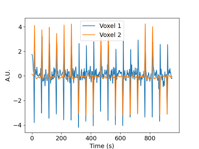
(a) Deoxyhemoglobin time courses

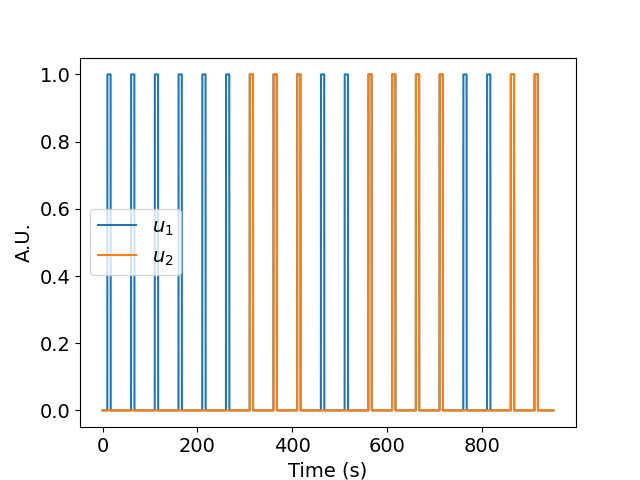
(b) Event time courses

Figure 1: Exemplary Voxel time course without any SNR observation noise perturbations

2.5 Statistical Analysis

For VGP-CCM, we generate the null distribution of the coupling statistic using equation 2, substituting $P(\theta_{x}|X)$ and $P(\theta_{y}|Y)$ with our approximate distributions $Q(\theta_{x})$ and $Q(\theta_{y})$ respectively. $\tilde{Y}$ and $\tilde{X}$ are sampled from 30 permutations of the original time series $X$ and Y respectively. GP-CCM, on the other hand, has its null distribution generated from eq. 1 with its hyperparameters obtained as the maximum a posteriori point estimate from Q obtained in equation 5. An $\alpha=0.05$ is used as the threshold for significance in all tests when applied to eq. 6. Given the Rossler and Lorenz equations each have 3 variables, we perform 9 comparisons ($X_{i}\rightarrow Y_{1},X_{i}\rightarrow Y_{2},X_{i}\rightarrow Y_{3}$ for i in 1…3). Thus, we have 270 tests for each coupling value. We then calculate the specificity, a measure of proneness to type I errors, as $\frac{\text{N correctly accepted $H_{0}$}}{\text{N correctly accepted $H_{0}$ + N incorrectly rejected $H_{0}$}}$ [31]. This same procedure is applied to the neurovascular system, except 100 time series are realized, thus 100 tests for coupling results are performed.

3 Results

	GP-CCM		VGP-CCM
Chaotic System	L$\rightarrow$R	R$\rightarrow$L	L$\rightarrow$R	R$\rightarrow$L
$\epsilon=(0.00,0.00)$	172	94	0	3
$\epsilon=(0.00,0.20)$	203	62	0	62
$\epsilon=(0.00,0.50)$	22	248	1	158
$\epsilon=(2.00,0.00)$	270	0	207	0
$\epsilon=(4.00,0.00)$	270	0	210	0
Neurovascular System	$V_{1}\rightarrow V_{2}$	$V_{2}\rightarrow V_{1}$	$V_{1}\rightarrow V_{2}$	$V_{2}\rightarrow V_{1}$
$B=\begin{bmatrix}\rho_{11}&\rho_{12}\\ 0&\rho_{22}\end{bmatrix}$	75	25	60	6

Table 2: Table displaying the number of rejected $H_{o}$ for each coupling values and each directionality test for the chaotic systems (Rossler to Lorenz equations (R$\rightarrow$L),Lorenz to Rossler equations (L$\rightarrow$ R)) or the neurovascular system (Voxel 1 to Voxel 2 ($V_{1}\rightarrow V_{2}$) or Voxel 2 to Voxel 1 ($V_{2}\rightarrow V_{1}$). First 2 columns are results obtained from results either using point estimates of the hyperparameters (GP-CCM), while the last two columns are results using approximate posterior distributions over hyperparameters (VGP-CCM).

Table 2 displays the set of significance rates for various couplings values for the unidirectionally coupled Lorenz-Rossler systems and for the neurovascular system. For zero coupling, VGP-CCM has only rejects the null hypothesis in 3 out of 270 realizations, whereas GP-CCM rejects the null hypothesis all but 4 of its test. Furthermore, VGP-CCM is more conservative than GP-CCM in dictating whether to make a claim of significant coupling at low coupling values, thus VGP-CCM very rarely made a false directionality claim. For the case of detecting Rossler driving Lorenz coupling, VGP-CCM reports a specificity of 99.6% while GP-CCM reports a specificity of 58.3%. In the direction from Lorenz driving Rossler, GP-CCM and VGP-CCM both report a specificity of 100%. For correctly rejecting the hypothesis in either direction, VGP-CCM has a specificity of 99.8% compared to GP-CCM’s 79.1%. Similarly for the neurovascular systems, the proposed variational VGP-CCM provides more specificity at 94% compared to GP-CCM’s 75%.

Fig. 2 displays cumulative distributions for simulating a Lorenz system of equations driving Rossler equations for coupling values $\epsilon=\{(0,0),(2,0)\}$ between variables X0 and Y0. The cumulative distribution reveals a robust null distribution when using the approximate posterior compared to using fixed values for the hyperparameters and performing permutations where results from only permuting samples results in a degenerate distribution with a collapsed mode. Both GP-CCM and VGP-CCM have an increasing raw coupling statistic as the coupling value increases.

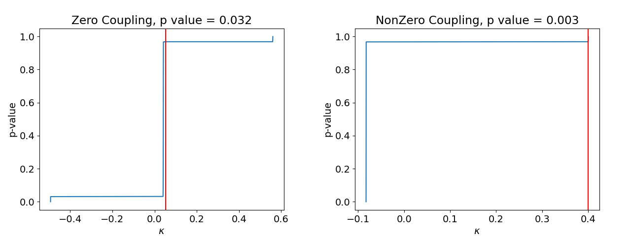
(a) Original GP-CCM method

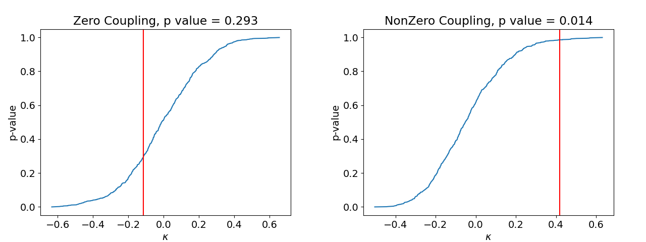
(b) Variational GP-CCM method

Figure 2: Example null distributions and p values for zero and non zero coupling seen from the Lorenz system to the Rossler system using the original GP-CCM method (a) and the proposed variational GP-CCM method (b). The value for nonpermuted maximum a posteriori time series results is shown in red

4 Discussion

We propose the VGP-CCM framework, which extends the GP-CCM to use a variational approximation to the posterior distribution of hyperparameters. The presented study aimed to use a variational approximation to the posterior distribution of hyperparameters to develop a more parsimonious distribution for testing a null uncoupled hypothesis for GP-CCM. Tests were performed on simulated unidirectionally coupled Lorenz-Rossler systems to control the values of coupling between the variables of the system of equations to determine whether GP-CCM and VGP-CCM suffered from false positives in the significance tests and at what coupling could either make significance statements. Neurovascular systems were also simulated to illustrate VGP-CCM’s efficacy at uncovering coupling in more slowly oscillating nonlinear signals compared to the chaotic maps studied in the Lorenz-Rossler system.

From the results over 30 realizations, as seen in table 2, VGP-CCM has much improved results compared to GP-CCM, with nearly 20% greater specificity than GP-CCM. Furthermore, from the simulations of the neurovascular system, we demonstrated that the proposed variational extension continues to provide further robustness even for slow oscillating signals as observed in deoxyhemoglobin signals, again with a similar substantial increase in specificity. As mentioned in the introduction, indeed the degenerate nature of the null distribution, as seen in fig 2a, allowed too much liberty to make claims of significance even in the wrong direction. This proves promising in the case that even in low coupling, VGP-CCM will not make a claim to the wrong direction, giving researchers confidence in the results that if the raw statistic is insignificant but with high value, it may be a matter of needing to collect more realizations, as seen in the low couplings values in table 2.

The prior distribution used in this study were indeed uninformative naively, though they allowed ease of computations, reparameterizations of means and variations with unit Gaussian random sample draws for automatic differentiation, and provided domain constraints. We suggest in studies where domain knowledge of how samples should a priori correlate is available, such as a kernel derived from mechanistic dynamic equations–e.g. time constants in linear ordinary differential equations as performed in dynamic causal modeling [32] or temperature in thermodynamic heat systems[33]–could be used. Otherwise, a separate dataset with labels can be used to infer optimal distributions through cross-validations. Even further directions may consider generative models for the posterior distribution conditioned on data, such as neural networks[23, 17].

From this study, we can conclude that integrating out the hyperparameters from the GP-CCM probability ratio may result in a more parsimonious statistic giving robust null distributions for hypothesis testings. The computational aspects are lessened by avoiding Markov Chain Monte Carlo integration on the true conditional a posteriori distribution, instead opting for variational approximations of the hyperparameter distribution with independent mean field structures. The robustness was verified on simulated data from unidirectional Lorenz-Rossler systems, where VGP-CCM achieved much higher specificity than GP-CCM. Further studies will look into applying this methodology on real world data such as neurophysiological systems.

5 Acknowledgments

The research leading to these results has received partial funding from the European Commission - Horizon 2020 Program under grant agreement n° 813234 of the project “RHUMBO”, and by Italian Ministry of Education and Research (MIUR) in the framework of the CrossLab project (Departments of Excellence).

References

- [1] T. Stankovski, T. Pereira, P. V. E. McClintock, and A. Stefanovska, “Coupling functions: Universal insights into dynamical interaction mechanisms,” Rev. Mod. Phys., vol. 89, p. 045001, Nov 2017.
- [2] K. J. Friston, “Functional and effective connectivity: a review.,” Brain connectivity, vol. 1, no. 1, pp. 13–36, 2011.
- [3] C. Granger, “Investigating causal relations by econometric models and cross-spectral methods,” Econometrica, vol. 37, no. 3, pp. 424–38, 1969.
- [4] T. Schreiber, “Measuring information transfer,” Phys. Rev. Lett., vol. 85, pp. 461–464, Jul 2000.
- [5] L. Barnett, A. B. Barrett, and A. K. Seth, “Granger causality and transfer entropy are equivalent for gaussian variables,” Phys. Rev. Lett., vol. 103, p. 238701, Dec 2009.
- [6] D. Marinazzo, M. Pellicoro, and S. Stramaglia, “Kernel method for nonlinear granger causality,” Phys. Rev. Lett., vol. 100, p. 144103, Apr 2008.
- [7] D. A. Smirnov and B. P. Bezruchko, “Spurious causalities due to low temporal resolution: Towards detection of bidirectional coupling from time series,” vol. 100, p. 10005, oct 2012.
- [8] D. A. Smirnov, “Spurious causalities with transfer entropy,” Phys. Rev. E, vol. 87, p. 042917, Apr 2013.
- [9] K. R. Popper, “Science as falsification,” Conjectures and refutations, vol. 1, no. 1963, pp. 33–39, 1963.
- [10] G. Sugihara, R. May, H. Ye, C.-h. Hsieh, E. Deyle, M. Fogarty, and S. Munch, “Detecting causality in complex ecosystems,” Science, vol. 338, no. 6106, pp. 496–500, 2012.
- [11] F. Takens, “Detecting strange attractors in turbulence,” in Dynamical Systems and Turbulence, Warwick 1980 (D. Rand and L.-S. Young, eds.), (Berlin, Heidelberg), pp. 366–381, Springer Berlin Heidelberg, 1981.
- [12] G. Feng, K. Yu, Y. Wang, Y. Yuan, and P. M. Djurić, “Improving convergent cross mapping for causal discovery with gaussian processes,” in ICASSP 2020 - 2020 IEEE International Conference on Acoustics, Speech and Signal Processing (ICASSP), pp. 3692–3696, 2020.
- [13] G. Feng, J. G. Quirk, and P. M. Djurić, “Detecting causality using deep gaussian processes,” in 2019 53rd Asilomar Conference on Signals, Systems, and Computers, pp. 472–476, 2019.
- [14] A. Ghouse, L. Faes, and G. Valenza, “Inferring directionality of coupled dynamical systems using gaussian process priors: Application on neurovascular systems,” Phys. Rev. E, vol. 104, p. 064208, Dec 2021.
- [15] C. E. Rasmussen and C. K. I. Williams, Gaussian Processes for Machine Learning (Adaptive Computation and Machine Learning). The MIT Press, 2005.
- [16] Y. Chung, A. Gelman, S. Rabe-Hesketh, J. Liu, and V. Dorie, “Weakly informative prior for point estimation of covariance matrices in hierarchical models,” Journal of Educational and Behavioral Statistics, vol. 40, no. 2, pp. 136–157, 2015.
- [17] D. M. Blei, A. Kucukelbir, and J. D. McAuliffe, “Variational inference: A review for statisticians,” Journal of the American Statistical Association, vol. 112, no. 518, pp. 859–877, 2017.
- [18] T. Sauer, J. A. Yorke, and M. Casdagli, “Embedology,” Journal of Statistical Physics, vol. 65, pp. 579–616, Nov 1991.
- [19] G. Sugihara and R. M. May, “Nonlinear forecasting as a way of distinguishing chaos from measurement error in time series,” Nature, vol. 344, no. 6268, pp. 734–741, 1990.
- [20] S. Geman and D. Geman, “Stochastic relaxation, gibbs distributions, and the bayesian restoration of images,” IEEE Transactions on pattern analysis and machine intelligence, no. 6, pp. 721–741, 1984.
- [21] M. J. Beal, Variational Algorithms for Approximate Bayesian Inference. PhD thesis, Gatsby Computational Neuroscience Unit, University College London, 2003.
- [22] S. Kullback and R. A. Leibler, “On Information and Sufficiency,” The Annals of Mathematical Statistics, vol. 22, no. 1, pp. 79 – 86, 1951.
- [23] D. J. C. MacKay, Bayesian Methods for Backpropagation Networks, pp. 211–254. New York, NY: Springer New York, 1996.
- [24] E. Snelson and Z. Ghahramani, “Sparse gaussian processes using pseudo-inputs,” in Proceedings of the 18th International Conference on Neural Information Processing Systems, NIPS’05, (Cambridge, MA, USA), p. 1257–1264, MIT Press, 2005.
- [25] D. P. Kingma and M. Welling, “Auto-Encoding Variational Bayes,” in 2nd International Conference on Learning Representations, ICLR 2014, Banff, AB, Canada, April 14-16, 2014, Conference Track Proceedings, 2014.
- [26] S. Y. Lee, “Gibbs sampler and coordinate ascent variational inference: A set-theoretical review,” Communications in Statistics - Theory and Methods, vol. 0, no. 0, pp. 1–21, 2021.
- [27] A. Paszke, S. Gross, S. Chintala, G. Chanan, E. Yang, Z. DeVito, Z. Lin, A. Desmaison, L. Antiga, and A. Lerer, “Automatic differentiation in pytorch,” 2017.
- [28] Y. Kim, S. Wiseman, A. C. Miller, D. A. Sontag, and A. M. Rush, “Semi-amortized variational autoencoders.,” in ICML (J. G. Dy and A. Krause, eds.), vol. 80 of Proceedings of Machine Learning Research, pp. 2683–2692, PMLR, 2018.
- [29] K. E. Stephan, N. Weiskopf, P. M. Drysdale, P. A. Robinson, and K. J. Friston, “Comparing hemodynamic models with dcm,” Neuroimage, vol. 38, no. 3, pp. 387–401, 2007.
- [30] K. Friston, “Dynamic causal modeling and granger causality comments on: The identification of interacting networks in the brain using fmri: Model selection, causality and deconvolution,” Neuroimage, vol. 58, no. 2-2, p. 303, 2011.
- [31] G. M. Gaddis and M. L. Gaddis, “Introduction to biostatistics: Part 3, sensitivity, specificity, predictive value, and hypothesis testing,” Annals of Emergency Medicine, vol. 19, no. 5, pp. 591–597, 1990.
- [32] K. Friston, L. Harrison, and W. Penny, “Dynamic causal modelling,” NeuroImage, vol. 19, no. 4, pp. 1273–1302, 2003.
- [33] N. Berline, E. Getzler, and V. Michèle, Heat kernels and Dirac operators. Springer, 1996.
- [34] A. Papoulis and S. U. Pillai, Probability, Random Variables, and Stochastic Processes. Boston: McGraw Hill, fourth ed., 2002.