The Application of Accumulation Test in Peaks Over Threshold Modeling with Norwegian Fire Insurance Data
Abstract
Modeling excess remains to be an important topic in insurance data modeling. Among the alternatives to modeling excess, the Peaks Over Threshold (POT) framework with Generalized Pareto distribution (GPD) is regarded as an efficient approach due to its flexibility. However, selecting an appropriate threshold for such a framework is a major difficulty. To address such difficulty, we applied several accumulation tests along with Anderson-Darling test to determine an optimal threshold. Limited simulations were conducted to assess the performance of accumulation tests. Based on the selected thresholds, the fitted GPD with the estimated quantiles can be found. We applied the procedure to the well-known Norwegian Fire Insurance data and constructed the confidence intervals for the Value-at-Risks (VaR). The accumulation test approach provides satisfactory performance in modeling the high quantiles of Norwegian Fire Insurance data compared to the previous graphical methods.
keywords:
Generalized Pareto Distribution\sepSequential Selection Procedure\sepPeaks Over Threshold Modeling\sepTail Risk Estimation\sepAccumulation Tests,
1 Introduction
The selection of a proper risk modeling approach is a major topic in the insurance industry. Among all existing approaches, parametric modeling is preferred due to its flexibility and interpretability. Within parametric methods, the Peaks Over Threshold (POT) approach with Generalized Pareto Distribution (GPD) remains popular due to the support of the Pickands–Balkema–De Haan theorem McNeil (\APACyear1997). However, the performance of such approach is mainly determined by the selection of thresholds. If the threshold is chosen to be too low, the excess distribution might not be well approximated by the GPD; If the threshold is chosen to be too high, number of excesses would not be enough to establish a useful model.
To identify an appropriate threshold in GPD modeling, many different methods have been proposed in the literature (Langousis \BOthers., \APACyear2016; Scarrott \BBA MacDonald, \APACyear2012, see). Gertensgarbe-Werner (GW) plot was first developed to identify the change point that separates non-extreme and extreme parts of the data Gerstengarbe \BBA Werner (\APACyear1989). However, the uniform assumption on the data of this method is an essential limitation. Therefore, this method should be avoided in real applications Langousis \BOthers. (\APACyear2016). Mean Residual Life (MRL) plot was also widely used to determine the GPD thresholds Davison \BBA Smith (\APACyear1990); Lang \BOthers. (\APACyear1999); Coles (\APACyear2001). This method aims to identify the threshold by looking for the linear trend of the candidate thresholds on the GPD parameters. However, the selection of threshold is usually done by a visual inspection, which is subjective. Compared to the methods mentioned above, threshold selection procedures with Goodness-of-Fit (GoF) tests could be interpreted with better support from statistical theory.
The objective of the GPD threshold selection procedures based on the GoF tests is to identify the lowest threshold such that the exceedances above the threshold fit a GPD well. For a single fixed threshold, the GoF test could be easily carried out Choulakian \BBA Stephens (\APACyear2001). However, a candidate set of possible thresholds are usually involved while finding the ’optimal’ threshold. Thus, error control is necessary since the candidate thresholds are tested simultaneously, which generates a multiple-testing problem. Due to the natural ordering of the candidate thresholds, the hypotheses for the GoF tests should also be ordered. Therefore, the False Discovery Rate (FDR) control procedures such as the Benjamini-Hochberg Benjamini \BBA Hochberg (\APACyear1995) or Benjamini-Yekutieli Benjamini \BBA Yekutieli (\APACyear2001) cannot be used without modifications. To adapt the FDR control procedures to the ordered hypotheses testing structure, G’Sell \BOthers. (\APACyear2016) proposed a procedure named ForwardStop. ForwardStop provides a way to choose a stopping point for ordered hypotheses such that the hypotheses occur before the stopping point can be rejected with adequate error control. Bader \BOthers. (\APACyear2018) then adapted this procedure to the selection of GDP thresholds with the application to the rainfall data.
The accumulation tests Li \BBA Barber (\APACyear2017) could be seen as a generalization of the ForwardStop procedure. Li \BBA Barber (\APACyear2017) showed that, any functions that satisfy certain regularity conditions could be utilized in the ordered hypotheses testing procedure with the FDR control at a desired level. In addition to ForwardStop, procedures like SeqStep Barber \BBA Candès (\APACyear2015) or HingeExp Li \BBA Barber (\APACyear2017) could also control FDR under different scenarios.
In this paper, we attempted to adapt both SeqStep and HingExp procedures to the GPD threshold selection problems, with an application to the Norwegian fire insurance data. The rest of the paper is organized as follows: In section 2, an introduction of GPD model and POT method was given, with a brief introduction of accumulation tests for sequential hypotheses testing. Section 3 provides simulations to assess the performance of different accumulation tests in selecting GPD thresholds. The real data analysis of the Norwegian fire insurance data set is given in Section 4. The final section concludes with a discussion and our thoughts about the future directions.
2 Methodology
2.1 POT Modeling and Threshold Selection Procedure
A common practice in extreme value modeling is to apply the Peaks Over Threshold (POT) approach to the exceedances beyond a certain threshold . This approach is built upon the second theorem of extreme value theory (the Pickands-Balkema-De Haan theorem). Under appropriate regularity conditions, the conditional excess function of a sequence of i.i.d. random variable can be well approximated by a Generalized Pareto Distribution with location parameter . A Generalized Pareto distribution is defined with the following cumulative distribution function (CDF):
| (1) |
where . When , the GPD distribution is defined as an exponential distribution with parameter .
The choice of is important in establishing a valuable model when applying the POT method. By the second theorem of the extreme value theory, the exceedances over the sufficiently high threshold follow a GPD approximately. However, if the threshold is chosen to be too high, the corresponding fitted GPD model would have a poor ability to describe the data distribution.
Let be a random sample of size . Assume this random sample is taken such that the regularity conditions for the Pickand-Balkema-De Haan theorem hold. Then, for an appropriate threshold , the exceedances approximately follows a GPD. Thus, the objective is to identify the lowest possible such that the exceedances approximately follow GPD.
2.2 MLE of and when is known
Suppose the threshold is known and both and are unknown. Suppose is fixed, let for . The log-likelihood of is as follows:
| (2) |
Essentially, the maximum of the likelihood function can be obtained:
Davison showed that the solution of the above system of equations can be reduced to finding the solution of equation with one variable, with the following steps Davison \BBA Smith (\APACyear1990):
-
1.
Let . The log-likelihood function becomes:
(3) -
2.
For any fixed value of , the ML estimate of the given is determined by :
(4) .
- 3.
-
4.
Eventually, the estimates of and can be expressed as follows, given the estimate of has been determined by maximizing Equation 5 numerically:
(6)
Grimshaw showed that the MLE for and might not exist in some situations Grimshaw (\APACyear1993). However, Choulakian pointed out that this is not likely to occur especially when the sample size is large enough Choulakian \BBA Stephens (\APACyear2001). Under most of the scenarios, the MLE of and can be obtained with the procedure introduced earlier in this subsection.
2.3 Goodness-of-Fit (GoF) Tests for GPD with Anderson-Darling Statistics
In order to assess the performance of the GPD fit, several tests were developed generally based on the GoF tests such as Anderson-Darling (AD) test. The details for the AD test are provided as follows: Given a sample is arranged in increasing order as , AD test statistic for the uniform distribution is defined as:
| (7) |
Therefore, to use the AD test for assessing the GoF of any distribution with the CDF properly defined, one could always use the probability integral transformation () on the ordered sample first and apply the AD test for the uniform distribution. Notice is the MLE of the parameter under .
2.4 Existing Method: Automated Threshold Selection Procedure
The automated threshold selection for the GPD was developed by utilizing an ordered hypothesis testing procedure named ForwardStop G’Sell \BOthers. (\APACyear2016); Bader \BOthers. (\APACyear2018). The selection procedure for the GPD could be summarized as follows:
-
1.
Pick candidate thresholds as .
-
2.
For each (), shift the data by applying the transformation (). is the sample size. After the shift, only the non-negative s are reserved since only the data values beyond the threshold are used in the fitting of a GPD model. Denote the non-negative s as follows:
Therefore, with determined by each , The corresponding MLE of and ( and ) can be obtained by using the method introduced in section 2.2,
-
3.
Then, for each , the null hypothesis:
is drawn from a GPD distribution,
could be examined by using GoF tests. different p-values are obtained correspondingly.
-
4.
The largest index for the candidate thresholds to be rejected is determined by applying the ForwardStop procedure G’Sell \BOthers. (\APACyear2016) as follows:
(8) where is pre-specified before the selection procedure. is then the optimal threshold.
The above procedure could produce good estimates for the thresholds of GPD if the candidates are chosen properly. For instance, when modeling the rainfall data, Bader \BOthers. (\APACyear2018) selected the thresholds within the and the percentile of the rainfall data and obtained a good geographical explanation based on the results obtained from the automated threshold selection procedure.
2.5 Accumulation Tests
Li and Barber Li \BBA Barber (\APACyear2017) later generalized the results from different ordered hypothesis testing procedures G’Sell \BOthers. (\APACyear2016); Barber \BBA Candès (\APACyear2015) including ForwardStop. A family of accumulation tests were developed to choose a cutoff point such that first hypotheses are rejected, with a modified false discovery rate (FDR) being controlled. Assume hypotheses are ordered sequentially as with corresponding -values . An accumulation function is defined as an integrable nondecreasing function that maps to . Then an accumulation test associated with the function chooses the cutoff as:
where the hypotheses can be rejected at the pre-specified FDR level . Therefore, ForwardStop is essentially a special case of the accumulation test procedure when .
Therefore, if we use any function that satisfies the conditions for the accumulation functions, a generalized GPD threshold selection procedure can be implemented along with the automated threshold selection procedure developed by Bader Bader \BOthers. (\APACyear2018). The flow chart for the generalized GPD threshold selection procedure is summarized in Figure 1.
2.6 VaR and the interval estimation of VaR for GPD
The estimation of Value-at-Risk (VaR) is important for the insurance data modeling. For a loss random variable, VaR at the level of is defined as:
In the insurance industry, VaR is the amount of capital that one insurance company needs to maintain to prevent the company from bankruptcy due to very extreme claims. Given that a random variable follows a GPD given CDF in (1), the VaR of could be easily derived in the following form:
| (9) |
Therefore, for given , and , the ML estimate of is:
As we explained in section 2.2, the MLE of and could be obtained numerically for a given . Smith (\APACyear1984) proved that when , the MLE of and are asymptotically normal and efficient:
where . With the MLE of and , the asymptotic variance of could be derived from the multivariate Delta method. Consider , the gradient . By Delta method, has the asymptotic distribution , where
| (10) | ||||
| (11) |
. By utilizing Delta method, the asymptotic CI for is is given as:
| (12) |
where represents the quantile of a standard Gaussian random variable.
3 Simulation
3.1 Simulation Settings
To assess the performance of sequential testing procedures, we conducted limited simulations. Three different accumulation tests were assessed for our simulations. The accumulation functions of these three accumulation tests are provided as follows:
-
•
ForwardStop:
-
•
SeqStep:
-
•
HingeExp:
For the value of involved in SeqStep and HingExp, we selected as Li and Barber Li \BBA Barber (\APACyear2017) recommended in their work of accumulation tests. For the significance threshold , we selected and in the simulations.
3.2 Scenarios of composite density with GPD tails
To demonstrate the ability of accumulation tests in selecting the thresholds for a GPD distribution in a POT model, we generated samples from four parametric composite distributions. The composite distributions were widely used in the modeling of insurance claim sizes Cooray \BBA Ananda (\APACyear2005); scollnik_composite_2007; Scollnik2012ModelingWW; brazauskas_modeling_2016; grun2019; Liu \BBA Ananda (\APACyear2022\APACexlab\BCnt1, \APACyear2022\APACexlab\BCnt2); mutali_composite_2020; deng_bayesian_2019; ig_pareto; exp_pareto; calderin-ojeda_note_2018. The details of the simulation scenarios are listed in Table 1. For each scenario, replicates were generated.
The mean and the RMSE were used to assess the performances of three tests under all scenarios. The formula for RMSE is provided as follows:
where denotes the chosen threshold for the -th replicate, stands for the true threshold under each scenario, and is the number of replicates.
3.3 Simulation Results
The simulation results are presented in Table 1 () and Table 2 (). For all scenarios, ForwardStop showed great performance, while SeqStep and HingeExp provided unsatisfactory performance. Notice for all sequential testing procedures, the RMSE decrease as the sample size increases.
| Scenario | True Threshold | Head Weight | Tail Weight | Sample Size |
|
|
|
|||||||||
|---|---|---|---|---|---|---|---|---|---|---|---|---|---|---|---|---|
| Mean | RMSE | Mean | RMSE | Mean | RMSE | |||||||||||
| GPD | 0.5 | - | - | n = 100 | 0.517 | 0.047 | 2.223 | 1.042 | 5.273 | 1.692 | ||||||
| n = 200 | 0.514 | 0.041 | 2.012 | 0.876 | 4.973 | 1.474 | ||||||||||
| n = 500 | 0.508 | 0.007 | 1.842 | 0.516 | 4.549 | 1.025 | ||||||||||
| GPD | 0.5 | - | - | n = 100 | 2.020 | 0.013 | 3.333 | 0.665 | 8.664 | 2.118 | ||||||
| n = 200 | 2.016 | 0.009 | 3.307 | 0.487 | 8.177 | 1.764 | ||||||||||
| n = 500 | 2.009 | 0.003 | 3.255 | 0.182 | 7.912 | 0.781 | ||||||||||
| lognormal, GPD | 2 | 0.3 | 0.7 | n = 100 | 1.941 | 0.080 | 5.575 | 1.133 | 9.497 | 1.549 | ||||||
| n = 200 | 1.953 | 0.069 | 4.892 | 0.984 | 8.768 | 1.376 | ||||||||||
| n = 500 | 1.981 | 0.091 | 4.137 | 0.582 | 7.642 | 1.058 | ||||||||||
| lognormal, GPD | 1 | 0.2 | 0.8 | n = 100 | 0.896 | 0.113 | 9.899 | 4.164 | 43.735 | 23.396 | ||||||
| n = 200 | 0.914 | 0.085 | 9.041 | 3.569 | 35.679 | 17.773 | ||||||||||
| n = 500 | 0.946 | 0.038 | 8.152 | 2.146 | 29.177 | 12.380 | ||||||||||
| Scenario | True Threshold | Head Weight | Tail Weight | Sample Size |
|
|
|
|||||||||
|---|---|---|---|---|---|---|---|---|---|---|---|---|---|---|---|---|
| Mean | RMSE | Mean | RMSE | Mean | RMSE | |||||||||||
| GPD | 0.5 | - | - | n = 100 | 0.662 | 0.056 | 3.126 | 1.242 | 7.134 | 1.719 | ||||||
| n = 200 | 0.597 | 0.050 | 2.124 | 0.772 | 6.171 | 1.351 | ||||||||||
| n = 500 | 0.568 | 0.011 | 1.939 | 0.572 | 5.813 | 0.997 | ||||||||||
| GPD | 0.5 | - | - | n = 100 | 2.514 | 0.021 | 3.992 | 0.785 | 12.178 | 2.375 | ||||||
| n = 200 | 2.423 | 0.015 | 3.687 | 0.512 | 10.045 | 1.891 | ||||||||||
| n = 500 | 2.291 | 0.011 | 3.491 | 0.195 | 9.912 | 0.748 | ||||||||||
| lognormal, GPD | 2 | 0.3 | 0.7 | n = 100 | 2.242 | 0.125 | 6.914 | 1.253 | 11.497 | 1.923 | ||||||
| n = 200 | 2.172 | 0.081 | 5.997 | 0.991 | 10.768 | 1.568 | ||||||||||
| n = 500 | 2.104 | 0.092 | 5.237 | 0.693 | 9.645 | 1.342 | ||||||||||
| lognormal, GPD | 1 | 0.2 | 0.8 | n = 100 | 1.196 | 0.146 | 10.891 | 3.928 | 33.614 | 15.463 | ||||||
| n = 200 | 1.131 | 0.103 | 10.141 | 3.261 | 31.436 | 13.616 | ||||||||||
| n = 500 | 1.074 | 0.047 | 9.352 | 2.646 | 27.377 | 11.453 | ||||||||||
4 Real Data Application: Threshold Selection
In this section, the well-known Norwegian Fire Insurance data is used to assess the performance of the different methods of the GPD threshold selection.
4.1 Data
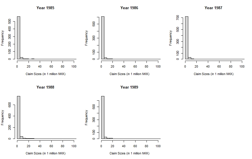
To illustrate the performance of the accumulation tests on the GPD threshold selection problems, we utilized the Norwegian Fire Insurance Data. The data set contains the fire insurance claims from a Norwegian company from year 1972 to 1992. The dataset is available via the R package ’ReIns’ Reynkens \BBA Verbelen (\APACyear2020). No information regarding inflation adjustments was provided so we chose the claims from year 1985 to 1989. Moreover, only the damages over 500,000 Norwegian Krones (NKK) are available. For analysis concern, we scaled the data by 1,000,000. The summary statistics of the claims from year 1985 to 1989 are presented in Table 3. Histograms of the claim sizes from 1985 to 1989 are presented in Figure 2.
| Year | Sample Size | Mean | SD | Q1 | Q2 | Q3 | Maximum |
|---|---|---|---|---|---|---|---|
| 1985 | 607 | 2.553 | 8.013 | 0.680 | 1.000 | 1.712 | 135.080 |
| 1986 | 647 | 2.477 | 9.695 | 0.700 | 0.985 | 1.549 | 188.270 |
| 1987 | 767 | 2.057 | 3.644 | 0.755 | 1.138 | 1.853 | 44.926 |
| 1988 | 827 | 3.176 | 17.677 | 0.762 | 1.176 | 2.049 | 465.365 |
| 1989 | 718 | 2.400 | 7.094 | 0.751 | 1.183 | 1.996 | 145.156 |
4.2 Selection of Accumulation Functions and Methods for Comparison
The accumulation tests that we chose in the simulations were applied to the Norwegian fire insurance data set. In addition, we selected two most commonly-used methods (GW plot and MRL plot) for comparison purposes. We utilized the R packages "tea" and "eva" to construct the plots and select the GPD thresholds.
4.3 Result: Threshold Selection
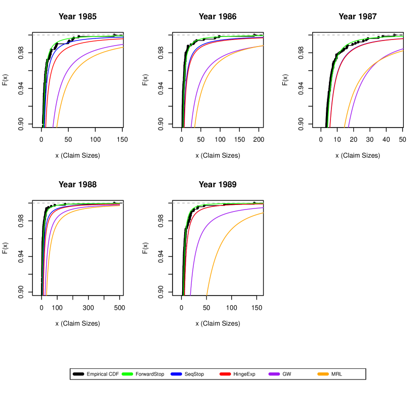
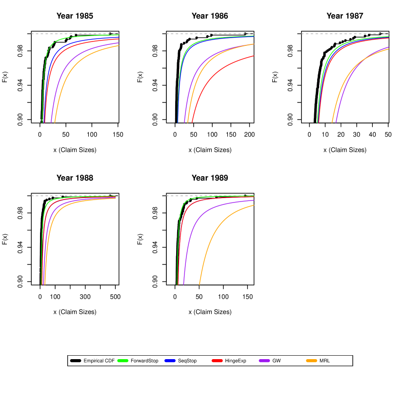
Table 4 presents the selection of the GPD thresholds , the corresponding MLE of the scale parameter and the shape parameter for the Norwegian Fire Insurance Data with the GW plot and the MRL plot; Table 5, 6 and 7 demonstrate the selection of the GPD thresholds , the corresponding MLE of the scale parameter and the shape parameter for the Norwegian Fire Insurance Data with the ForwardStop selection, the SeqStep selection and HingeExp selection. Notice the GW plot and the MRL plot methods provided higher estimates for compared to the selection methods based on the accumulation tests. With these estimates, we were able to create the estimated CDFs of the GPD for the Norwegian Fire Insurance Data, with the different threshold selection methods. Comparisons of the estimated CDFs and the empirical CDFs for the Norwegian Fire Insurance Data are demonstrated in Figures 3 and 4.
We noticed that the estimated CDFs using the threshold selection with accumulation tests are closer to the empirical CDFs than the graphical methods over all the years we selected from the Norwegian Fire Insurance Data. This implies that the accumulation tests have a stronger ability to detect the appropriate thresholds compared to the graphical methods, with the GPD assumptions. Among three accumulation tests, the ForwardStop selection provided the closest fits to the empirical CDFs. Notice if we compare Tables 5, 6 and 7, the selected thresholds with ForwardStop are significantly lower compared to the selected thresholds with HingeExp or SeqStep. This could be relevant since, as mentioned in Section 3.1, only claims with very high values (over 500,000 NKKs) are available. Given the data is obtained in this way, it is likely that the distribution of most of the claims over 500,000 NKKs could be modeled appropriately using GPD, based on the second theorem of extreme theory. Since the ForwardStop selection provided the lowest thresholds among all of the methods mentioned in this study, it obviously includes more claims for GPD modeling in comparison to other methods that chose higher thresholds. Thus, it is reasonable that the ForwardStop selection provided the closest fits to empirical CDFs comapred to all other methods.
It is also notable that the choices of the false discovery proportion have impacts on the selection of the thresholds. With the accumulation tests, (Figure 3) provides better fits to the emiprical CDF compared to (Figure 4), especially for year 1986 and 1987. A possible explanation is that, when is set to be low, the thresholds would be detected earlier based on what was described in section 2.5. Therefore, with the nature of the Norwegian Fire Insurance Data being truncated at 0.5 million NKK, apparently produces the thresholds closer to the truncated point, and hence leads to a closer fit to the data in comparison with .
| Method | Year | Chosen Threshold () | Scale () | Shape () |
|---|---|---|---|---|
| GW Plot | 1985 | 2.570 | 2.764 | 0.843 |
| 1986 | 3.363 | 2.460 | 1.010 | |
| 1987 | 3.499 | 3.014 | 0.536 | |
| 1988 | 3.331 | 3.010 | 0.795 | |
| 1989 | 3.062 | 2.532 | 0.734 | |
| MRL Plot | 1985 | 3.500 | 3.854 | 0.810 |
| 1986 | 4.500 | 4.356 | 0.838 | |
| 1987 | 3.000 | 1.998 | 0.716 | |
| 1988 | 5.000 | 4.388 | 0.766 | |
| 1989 | 8.500 | 10.797 | 0.441 |
| Year | Chosen Threshold () | Scale () | Shape () | |
|---|---|---|---|---|
| 0.01 | 1985 | 0.541 | 0.558 | 0.769 |
| 1986 | 0.677 | 0.539 | 0.798 | |
| 1987 | 0.660 | 0.757 | 0.554 | |
| 1988 | 0.745 | 0.768 | 0.768 | |
| 1989 | 0.531 | 0.764 | 0.567 | |
| 0.05 | 1985 | 0.577 | 0.524 | 0.823 |
| 1986 | 1.079 | 0.655 | 0.970 | |
| 1987 | 0.974 | 0.770 | 0.662 | |
| 1988 | 0.973 | 0.871 | 0.811 | |
| 1989 | 0.555 | 0.751 | 0.584 |
| Year | Chosen Threshold () | Scale () | Shape () | |
| 0.01 | 1985 | 0.862 | 0.677 | 0.874 |
| 1986 | 1.079 | 0.655 | 0.970 | |
| 1987 | 1.086 | 0.816 | 0.677 | |
| 1988 | 1.248 | 0.918 | 0.909 | |
| 1989 | 1.138 | 0.897 | 0.698 | |
| 0.05 | 1985 | 1.193 | 0.876 | 0.921 |
| 1986 | 1.152 | 0.688 | 0.997 | |
| 1987 | 1.104 | 0.818 | 0.682 | |
| 1988 | 1.590 | 1.388 | 0.846 | |
| 1989 | 1.170 | 0.870 | 0.726 |
| Year | Chosen Threshold () | Scale () | Shape () | |
|---|---|---|---|---|
| 0.01 | 1985 | 1.214 | 0.885 | 0.926 |
| 1986 | 1.152 | 0.688 | 0.997 | |
| 1987 | 1.104 | 0.818 | 0.682 | |
| 1988 | 1.590 | 1.388 | 0.846 | |
| 1989 | 1.138 | 0.897 | 0.698 | |
| 0.05 | 1985 | 1.378 | 0.894 | 1.004 |
| 1986 | 6.972 | 3.524 | 1.152 | |
| 1987 | 1.185 | 0.832 | 0.706 | |
| 1988 | 1.659 | 1.533 | 0.814 | |
| 1989 | 1.183 | 0.895 | 0.717 |
4.4 Result: Measuring Tail Risk using VaR
Table 8, 9, 10 and 11 provides the estimates of VaRs at the percent level and the percent level, along with the asymptotic 95% CIs of the VaRs. We labelled the CIs that does not cover the empirical VaRs with red color. Similar to what we described in section 3.3, the accumulation tests (in Tables 9, 10 and 11) generally produced closer estimates to the empirical VaRs compared to the previous graphical methods (in Table 8) over all the years. In addition, notice when using the previous graphical methods, all the asymptotic 95% CIs for the VaRs did not cover the corresponding empirical estimates. This implies the graphical methods generally could not provide satisfactory fittings for the high quantiles.
The 95% asymptotic CIs for VaRs were computed based on the Delta method described in section 2.6. We labeled a CI in red color if the CI does not cover the corresponding empirical VaR estimate. We noticed that the CIs produced from the ForwardStop selection covered almost all the empirical VaR estimates. This implies the ForwardStop selection has the best ability to model the high quantiles of the claim size distributions in comparison with the SeqStep and HingeExp selections.
| Year | Method | VaR(0.90) (95% CI) | VaR(0.95) (95% CI) |
|---|---|---|---|
| 1985 | Empirical | 3.50 | 7.15 |
| GW | 22.13 (18.92, 25.35) | 40.26 (33.89, 46.84) | |
| MRL | 29.46 (25.40, 33.53) | 52.60 (44.81, 66.39) | |
| 1986 | Empirical | 3.34 | 6.97 |
| GW | 25.85 (21.84, 29.86) | 51.12 (42.09, 60.15) | |
| MRL | 35.10 (30.45, 39.75) | 63.29 (54.26, 72.33) | |
| 1987 | Empirical | 3.52 | 6.04 |
| GW | 17.19 (15.46, 18.93) | 25.89 (23.02, 28.75) | |
| MRL | 14.72 (16.09, 20.52) | 24.04 (20.88, 27.21) | |
| 1988 | Empirical | 4.55 | 7.72 |
| GW | 23.16 (20.46, 25.86) | 40.52 (35.35, 45.69) | |
| MRL | 32.69 (29.06, 36.32) | 56.11 (49.35, 62.86) | |
| 1989 | Empirical | 3.86 | 6.19 |
| GW | 18.31 (16.10, 20.52) | 30.71 (26.60, 34.82) | |
| MRL | 51.60 (46.25, 56.96) | 75.77 (67.40, 84.13) |
-
*
Red color indicates the CI does not cover the corresponding empirical VaR estimate.
| Year | VaR(0.90) (95% CI) | VaR(0.95) (95% CI) | |
|---|---|---|---|
| 1985 | Empirical | 3.50 | 7.15 |
| 0.01 | 4.07 (2.34, 5.81) | 7.08 (2.93, 11.23) | |
| 0.05 | 4.18 (1.92, 6.44) | 7.43 (1.77, 13.10) | |
| 1986 | Empirical | 3.34 | 6.97 |
| 0.01 | 4.24 (2.31, 6.18) | 7.32 (2.63, 12.13) | |
| 0.05 | 6.71 (3.29, 10.12) | 12.75 (3.41, 22.08) | |
| 1987 | Empirical | 3.52 | 6.04 |
| 0.01 | 4.19 (3.54, 4.84) | 6.48 (5.26, 7.70) | |
| 0.05 | 5.15 (4.22, 6.08) | 8.26 (6.33, 10.19) | |
| 1988 | Empirical | 4.55 | 7.72 |
| 0.01 | 5.61 (4.30, 6.91) | 9.73 (6.76, 12.70) | |
| 0.05 | 6.85 (5.36, 8.34) | 12.09 (8.67, 15.52) | |
| 1989 | Empirical | 3.86 | 6.19 |
| 0.01 | 4.16 (3.45, 4.86) | 6.55 (5.22, 7.88) | |
| 0.05 | 4.20 (3.46, 4.94) | 6.67 (5.24, 8.09) |
-
*
Red color indicates the CI does not cover the corresponding empirical VaR estimate.
| Year | VaR(0.90) | VaR(0.95) | |
|---|---|---|---|
| 1985 | Empirical | 3.50 | 7.15 |
| 0.01 | 5.88 (3.50, 8.26) | 10.71 (4.68, 16.74) | |
| 0.05 | 8.17 (5.63, 10.71) | 15.26 (8.84, 21.68) | |
| 1986 | Empirical | 3.34 | 6.97 |
| 0.01 | 6.71 (3.29, 10.12) | 12.75 (3.41, 22.08) | |
| 0.05 | 7.32 (3.65, 10.98) | 14.14 (3.96, 24.32) | |
| 1987 | Empirical | 3.52 | 6.04 |
| 0.01 | 5.61 (4.63, 6.59) | 9.04 (7.00, 11.08) | |
| 0.05 | 5.67 (4.67, 6.67) | 9.16 (7.08, 11.24) | |
| 1988 | Empirical | 4.55 | 7.72 |
| 0.01 | 8.43 (6.37, 10.49) | 15.62 (10.51, 20.73) | |
| 0.05 | 11.46 (9.70, 13.21) | 20.64 (16.84, 24.43) | |
| 1989 | Empirical | 3.86 | 6.19 |
| 0.01 | 6.26 (5.17, 7.36) | 10.25 (7.98, 12.53) | |
| 0.05 | 6.34 (5.15, 7.55) | 10.52 (7.95, 13.08) |
-
*
Red color indicates the CI does not cover the corresponding empirical VaR estimate.
| Year | VaR(0.90) | VaR(0.95) | |
|---|---|---|---|
| 1985 | Empirical | 3.50 | 7.15 |
| 0.01 | 8.32 (5.74, 10.89) | 15.57 (9.04, 22.10) | |
| 0.05 | 9.47 (6.10, 12.85) | 18.51 (9.41, 27.61) | |
| 1986 | Empirical | 3.34 | 6.97 |
| 0.01 | 7.32 (3.65, 10.98) | 14.14 (3.96, 24.32) | |
| 0.05 | 47.32 (40.25, 54.40) | 100.38(83.36,117.39) | |
| 1987 | Empirical | 3.52 | 6.04 |
| 0.01 | 5.67 (4.67, 6.67) | 9.16 (7.08, 11.24) | |
| 0.05 | 6.00 (4.91, 7.08) | 9.78 (7.48, 12.07) | |
| 1988 | Empirical | 4.55 | 7.72 |
| 0.01 | 11.46 (9.70, 13.21) | 20.64 (16.84, 24.43) | |
| 0.05 | 12.05 (10.35, 13.74) | 21.35 (17.84, 24.86) | |
| 1989 | Empirical | 3.86 | 6.19 |
| 0.01 | 6.26 (5.17, 7.36) | 10.25 (7.98, 12.53) | |
| 0.05 | 6.44 (5.27, 7.61) | 10.63 (8.17, 13.09) |
-
*
Red color indicates the CI does not cover the corresponding empirical VaR estimate.
5 Conclusion
In this article, three different accumulation tests have been used to generate the GPD models for claim size distributions and VaR estimates over the Norwegian Fire Insurance Data. Among the accumulation tests, the ForwardStop utilizes a smooth logarithmic function as the accumulation function while the SeqStep and the HingeExp employ a discrete step function with a pre-specified parameter as the accumulation function. We also used the previous graphical methods including GW-Plot and MRL-Plot to generate the models for comparison purposes. Among all the models, the ForwardStop selection demonstrates the best performance as it produces the closest fits to the empirical CDFs and the closest estimates to the empirical VaRs at the 90% and 95% level. The SeqStep and the HingeExp also performed better in comparison with previous graphical methods. Therefore, regarding the Norwegian Fire Insurance Data, the threshold selection methods based on the accumulation tests have better ability to capture the features of the claim size distributions compared to the previous widely-used methods.
The threshold selection based on the accumulation tests is attractive due to their good performance fitting the Norwegian Fire Insurance Data. However, one needs to take precautions in terms of the following: the quality of the modeling for the accumulation tests are affected by the chosen FDP (). For instance, the ForwardStop selection with generally overperformed the same procedure with . Hence, before using the accumulation tests, a reasonable selection on is necessary in order to obtain a better model, especially for modeling high quantiles. In addition, both SeqStep and HingeExp use a specific parameter that needs to be specified before the selection procedure. We did not test the effect of on the estimation of GPD modeling in this article. However, it definitely has an impact on the selection of thresholds since different will lead to different choices of the threshold , even with the same dataset.
Finally, we conclude that the accumulation tests have great ability to choose the thresholds in the GPD models for the Norwegian Fire Insurance Data. More extended uses and improvements for such method in the GPD modeling are warranted, especially producing tail risk measures other than VaR (e.g. tail conditional mean) by using the thresholds chosen by the accumulation tests.
References
- Bader \BOthers. (\APACyear2018) \APACinsertmetastarbader_automated_2018{APACrefauthors}Bader, B., Yan, J.\BCBL \BBA Zhang, X. \APACrefYearMonthDay2018\APACmonth03. \BBOQ\APACrefatitleAutomated threshold selection for extreme value analysis via ordered goodness-of-fit tests with adjustment for false discovery rate Automated threshold selection for extreme value analysis via ordered goodness-of-fit tests with adjustment for false discovery rate.\BBCQ \APACjournalVolNumPagesThe Annals of Applied Statistics121310–329. \APACrefnotePublisher: Institute of Mathematical Statistics {APACrefDOI} 10.1214/17-AOAS1092 \PrintBackRefs\CurrentBib
- Barber \BBA Candès (\APACyear2015) \APACinsertmetastarbarber_controlling_2015{APACrefauthors}Barber, R\BPBIF.\BCBT \BBA Candès, E\BPBIJ. \APACrefYearMonthDay2015\APACmonth10. \BBOQ\APACrefatitleControlling the false discovery rate via knockoffs Controlling the false discovery rate via knockoffs.\BBCQ \APACjournalVolNumPagesThe Annals of Statistics4352055–2085. \APACrefnotePublisher: Institute of Mathematical Statistics {APACrefDOI} 10.1214/15-AOS1337 \PrintBackRefs\CurrentBib
- Benjamini \BBA Hochberg (\APACyear1995) \APACinsertmetastarbenjamini_controlling_1995{APACrefauthors}Benjamini, Y.\BCBT \BBA Hochberg, Y. \APACrefYearMonthDay1995. \BBOQ\APACrefatitleControlling the False Discovery Rate: A Practical and Powerful Approach to Multiple Testing Controlling the False Discovery Rate: A Practical and Powerful Approach to Multiple Testing.\BBCQ \APACjournalVolNumPagesJournal of the Royal Statistical Society. Series B (Methodological)571289–300. \APACrefnotePublisher: [Royal Statistical Society, Wiley] \PrintBackRefs\CurrentBib
- Benjamini \BBA Yekutieli (\APACyear2001) \APACinsertmetastarbenjamini_control_2001{APACrefauthors}Benjamini, Y.\BCBT \BBA Yekutieli, D. \APACrefYearMonthDay2001\APACmonth08. \BBOQ\APACrefatitleThe control of the false discovery rate in multiple testing under dependency The control of the false discovery rate in multiple testing under dependency.\BBCQ \APACjournalVolNumPagesThe Annals of Statistics2941165–1188. \APACrefnotePublisher: Institute of Mathematical Statistics \PrintBackRefs\CurrentBib
- Choulakian \BBA Stephens (\APACyear2001) \APACinsertmetastarchoulakian_goodness–fit_2001{APACrefauthors}Choulakian, V.\BCBT \BBA Stephens, M\BPBIA. \APACrefYearMonthDay2001\APACmonth11. \BBOQ\APACrefatitleGoodness-of-Fit Tests for the Generalized Pareto Distribution Goodness-of-Fit Tests for the Generalized Pareto Distribution.\BBCQ \APACjournalVolNumPagesTechnometrics434478–484. \APACrefnotePublisher: Taylor & Francis _eprint: https://doi.org/10.1198/00401700152672573 {APACrefDOI} 10.1198/00401700152672573 \PrintBackRefs\CurrentBib
- Coles (\APACyear2001) \APACinsertmetastarcoles_threshold_2001{APACrefauthors}Coles, S. \APACrefYearMonthDay2001. \BBOQ\APACrefatitleThreshold Models Threshold Models.\BBCQ \BIn S. Coles (\BED), \APACrefbtitleAn Introduction to Statistical Modeling of Extreme Values An Introduction to Statistical Modeling of Extreme Values (\BPGS 74–91). \APACaddressPublisherLondonSpringer. \PrintBackRefs\CurrentBib
- Cooray \BBA Ananda (\APACyear2005) \APACinsertmetastarananda2005{APACrefauthors}Cooray, K.\BCBT \BBA Ananda, M\BPBIM\BPBIA. \APACrefYearMonthDay2005. \BBOQ\APACrefatitleModeling actuarial data with a composite lognormal-Pareto model Modeling actuarial data with a composite lognormal-pareto model.\BBCQ \APACjournalVolNumPagesScandinavian Actuarial Journal20055321-334. {APACrefDOI} 10.1080/03461230510009763 \PrintBackRefs\CurrentBib
- Davison \BBA Smith (\APACyear1990) \APACinsertmetastardavison_models_1990{APACrefauthors}Davison, A\BPBIC.\BCBT \BBA Smith, R\BPBIL. \APACrefYearMonthDay1990. \BBOQ\APACrefatitleModels for Exceedances over High Thresholds Models for Exceedances over High Thresholds.\BBCQ \APACjournalVolNumPagesJournal of the Royal Statistical Society. Series B (Methodological)523393–442. \APACrefnotePublisher: [Royal Statistical Society, Wiley] \PrintBackRefs\CurrentBib
- Gerstengarbe \BBA Werner (\APACyear1989) \APACinsertmetastargert_1989{APACrefauthors}Gerstengarbe, F.\BCBT \BBA Werner, P. \APACrefYearMonthDay1989Jan. \APACrefbtitleA method for the statistical definition of extreme-value regions and their application to meteorological time series A method for the statistical definition of extreme-value regions and their application to meteorological time series (\BVOL 39:4). \PrintBackRefs\CurrentBib
- Grimshaw (\APACyear1993) \APACinsertmetastargrimshaw_computing_1993{APACrefauthors}Grimshaw, S\BPBID. \APACrefYearMonthDay1993. \BBOQ\APACrefatitleComputing Maximum Likelihood Estimates for the Generalized Pareto Distribution Computing Maximum Likelihood Estimates for the Generalized Pareto Distribution.\BBCQ \APACjournalVolNumPagesTechnometrics352185–191. \APACrefnotePublisher: [Taylor & Francis, Ltd., American Statistical Association, American Society for Quality] {APACrefDOI} 10.2307/1269663 \PrintBackRefs\CurrentBib
- G’Sell \BOthers. (\APACyear2016) \APACinsertmetastargsell_sequential_2016{APACrefauthors}G’Sell, M\BPBIG., Wager, S., Chouldechova, A.\BCBL \BBA Tibshirani, R. \APACrefYearMonthDay2016. \BBOQ\APACrefatitleSequential selection procedures and false discovery rate control Sequential selection procedures and false discovery rate control.\BBCQ \APACjournalVolNumPagesJournal of the Royal Statistical Society. Series B (Statistical Methodology)782423–444. \APACrefnotePublisher: [Royal Statistical Society, Wiley] \PrintBackRefs\CurrentBib
- Lang \BOthers. (\APACyear1999) \APACinsertmetastarlang_towards_1999{APACrefauthors}Lang, M., Ouarda, T\BPBIB\BPBIM\BPBIJ.\BCBL \BBA Bobée, B. \APACrefYearMonthDay1999\APACmonth12. \BBOQ\APACrefatitleTowards operational guidelines for over-threshold modeling Towards operational guidelines for over-threshold modeling.\BBCQ \APACjournalVolNumPagesJournal of Hydrology2253103–117. {APACrefDOI} 10.1016/S0022-1694(99)00167-5 \PrintBackRefs\CurrentBib
- Langousis \BOthers. (\APACyear2016) \APACinsertmetastarlangousis_threshold_2016{APACrefauthors}Langousis, A., Mamalakis, A., Puliga, M.\BCBL \BBA Deidda, R. \APACrefYearMonthDay2016. \BBOQ\APACrefatitleThreshold detection for the generalized Pareto distribution: Review of representative methods and application to the NOAA NCDC daily rainfall database Threshold detection for the generalized Pareto distribution: Review of representative methods and application to the NOAA NCDC daily rainfall database.\BBCQ \APACjournalVolNumPagesWater Resources Research5242659–2681. \APACrefnote_eprint: https://agupubs.onlinelibrary.wiley.com/doi/pdf/10.1002/2015WR018502 \PrintBackRefs\CurrentBib
- Li \BBA Barber (\APACyear2017) \APACinsertmetastarli_accumulation_2017{APACrefauthors}Li, A.\BCBT \BBA Barber, R\BPBIF. \APACrefYearMonthDay2017\APACmonth04. \BBOQ\APACrefatitleAccumulation Tests for FDR Control in Ordered Hypothesis Testing Accumulation Tests for FDR Control in Ordered Hypothesis Testing.\BBCQ \APACjournalVolNumPagesJournal of the American Statistical Association112518837–849. \APACrefnotePublisher: Taylor & Francis _eprint: https://doi.org/10.1080/01621459.2016.1180989 {APACrefDOI} 10.1080/01621459.2016.1180989 \PrintBackRefs\CurrentBib
- Liu \BBA Ananda (\APACyear2022\APACexlab\BCnt1) \APACinsertmetastarliu_analyzing_2022{APACrefauthors}Liu, B.\BCBT \BBA Ananda, M\BPBIM\BPBIA. \APACrefYearMonthDay2022\BCnt1. \BBOQ\APACrefatitleAnalyzing insurance data with an exponentiated composite Inverse-Gamma Pareto Model Analyzing insurance data with an exponentiated composite Inverse-Gamma Pareto Model.\BBCQ \APACjournalVolNumPagesCommunications in Statistics - Theory and Methods. {APACrefDOI} 10.1080/03610926.2022.2050399 \PrintBackRefs\CurrentBib
- Liu \BBA Ananda (\APACyear2022\APACexlab\BCnt2) \APACinsertmetastarliu_generalized_2022{APACrefauthors}Liu, B.\BCBT \BBA Ananda, M\BPBIM\BPBIA. \APACrefYearMonthDay2022\BCnt2\APACmonth01. \BBOQ\APACrefatitleA Generalized Family of Exponentiated Composite Distributions A Generalized Family of Exponentiated Composite Distributions.\BBCQ \APACjournalVolNumPagesMathematics10111895. {APACrefDOI} 10.3390/math10111895 \PrintBackRefs\CurrentBib
- McNeil (\APACyear1997) \APACinsertmetastarmcneil_estimating_1997{APACrefauthors}McNeil, A\BPBIJ. \APACrefYearMonthDay1997\APACmonth05. \BBOQ\APACrefatitleEstimating the Tails of Loss Severity Distributions Using Extreme Value Theory Estimating the Tails of Loss Severity Distributions Using Extreme Value Theory.\BBCQ \APACjournalVolNumPagesASTIN Bulletin: The Journal of the IAA271117–137. \APACrefnotePublisher: Cambridge University Press {APACrefDOI} 10.2143/AST.27.1.563210 \PrintBackRefs\CurrentBib
- Reynkens \BBA Verbelen (\APACyear2020) \APACinsertmetastarreins{APACrefauthors}Reynkens, T.\BCBT \BBA Verbelen, R. \APACrefYearMonthDay2020. \BBOQ\APACrefatitleReIns: Functions from "Reinsurance: Actuarial and Statistical Aspects" Reins: Functions from "reinsurance: Actuarial and statistical aspects"\BBCQ [\bibcomputersoftwaremanual]. \APACrefnoteR package version 1.0.10 \PrintBackRefs\CurrentBib
- Scarrott \BBA MacDonald (\APACyear2012) \APACinsertmetastarscarrot{APACrefauthors}Scarrott, C.\BCBT \BBA MacDonald, A. \APACrefYearMonthDay201203. \BBOQ\APACrefatitleA review of extreme value threshold estimation and uncertainty quantification A review of extreme value threshold estimation and uncertainty quantification.\BBCQ \APACjournalVolNumPagesRevstat Statistical Journal1033-60. \PrintBackRefs\CurrentBib
- Smith (\APACyear1984) \APACinsertmetastarsmith_threshold_1984{APACrefauthors}Smith, R\BPBIL. \APACrefYearMonthDay1984. \BBOQ\APACrefatitleThreshold Methods for Sample Extremes Threshold Methods for Sample Extremes.\BBCQ \BIn J\BPBIT. de Oliveira (\BED), \APACrefbtitleStatistical Extremes and Applications Statistical Extremes and Applications (\BPGS 621–638). \APACaddressPublisherDordrechtSpringer Netherlands. \PrintBackRefs\CurrentBib