$4D$ AdS Einstein-Gauss-Bonnet black hole with Yang-Mills field and its thermodynamics

Abstract

We derive an exact black hole solution for the Einstein-Gauss-Bonnet gravity with Yang-Mills field in $4D$ AdS spacetime and investigate its thermodynamic properties to calculate exact expressions for the black hole mass, temperature, entropy and heat capacity. The thermodynamic quantities get modification in the presence of Yang-Mills field, however, entropy remains unaffected by the Yang-Mills charge. The solution exhibits $P\--v$ criticality and belongs to the universality class of Van der Waals fluid. We study the effect of Gauss-Bonnet coupling and Yang-Mills charge on the critical behaviour and black hole phase transition. We observe that the values of critical exponents increase with the Yang-Mills charge and decrease with the Gauss-Bonnet coupling constant.

I Introduction

Einstein theory of general relativity (GR) is one of the most successful theories in theoretical physics. Despite its appreciable achievements, there are still some unsolved problems in the universe such as the hierarchy problem, the cosmological constant problem, and the late time accelerated expansion of the Universe. This reflects that GR is not the ultimate theory and needs further generalization. One of the possible generalization for the standard Einstein-Hilbert action is by adding the higher curvature terms. Natural candidates for the higher curvature corrections are provided by Lovelock gravities, which are the unique theories that give rise to generally covariant field equations lav . Gauss-Bonnet gravity, also called as Einstein-Gauss-Bonnet (EGB), is the simplest extension of the Einstein-Hilbert action to include higher curvature Lovelock terms. A Gauss-Bonnet term appears naturally in the low energy effective action of string theory zwe .

Thermodynamic properties of black holes have been studied for many years hen ; sud4 ; sud5 ; sud6 ; sud7 and found that black hole spacetime can not only be assigned standard thermodynamic variables such as temperature or entropy, but were also shown to possess rich phase structures and admit critical phenomena. Hawking and Page haw were the first who studied the thermodynamic properties of AdS black holes and found the existence of a certain phase transition in the phase space of the (nonrotating uncharged) Schwarzschild-AdS black hole. This was the first order phase transition between thermal AdS space and the Schwarzschild-AdS black hole, with the latter becoming thermodynamically preferred above a certain critical temperature. The study of the phase transitions in higher curvature gravity are subject of present research 05 ; 06 ; 07 . For instance, Van der Waals behaviour, (multiple)-rentrant phase transitions, critical points and isolated critical points for a variety of asymptotically AdS black holes can be found in Refs. 08 ; 09 ; 10 ; 11 ; 12 ; 13 . Although there various black hole solutions exist, but the black hole solution for the EGB gravity with Yang-Mills field and their thermal properties remain unstudied. This provides us an opportunity to bridge this gap.

Recently, Glavan and Lin gla introduced the 4-dimensional theory of gravity with Gauss-Bonnet correction by re-scaling the Gauss-Bonnet coupling $\alpha\to\alpha/D-4$. Here, it is important to note that taking the limit $D\rightarrow 4$ after $\alpha\to\alpha/D-4$ either breaks part of diffeomorphism or leads to extra gravitational degrees of freedom. Clearly, both of these violate conditions of the Lovelock’s theorem lav . A consistent theory of $D\rightarrow 4$ EGB gravity with two dynamical degrees of freedom is proposed by breaking the temporal diffeomorphism invariance Ao1 ; Ao2 . The generalization to other spherically symmetric black holes has also discussed in Refs. fran ; Singh:2020nwo ; Hennigar:2020lsl . Other probes include studies of the regular black holes Singh:2020mty ; Yang:2020jno ; Kumar:2020uyz ; 32 ; 33 ; 35 ; 36 ; 37 , quasi-normal modes Devi:2020uac ; Mishra:2020gce , gravitational lensing Jin:2020emq ; Islam:2020xmy , thermodynamic properties, $P-v$ criticality and phase transition Konoplya:2020cbv ; Wei:2020poh ; Singh:2020xju ; Zhang:2020obn ; Singh20 ; Singh21 ; hendi19 ; hendi20 ; hendi18 ; hendi17 ; hendi16 ; he ; hendi2017 .

In this work, we first obtain a static spherically symmetric black hole solution for EGB gravity with Yang-Mills field. The solution by Glavan and Lin can be recovered from this generalized solution. Actually, the resulting solution interpolates with the Glavan and Lin solution gla in the Yang-Mills charge. In order to analyse thermodynamic property, we estimate the mass, Hawking temperature from area-law and entropy which satisfy the first-law of thermodynamics. The stability of the system is studied by computing the heat capacity. Here, we observe that the heat capacity curve is discontinuous at the critical radius. Further, we notice that there is a flip of sign in the heat capacity around critical radius. Thus, we can say that $4D$ EGB AdS Yang-Mills black holes whose horizon radius is smaller than the critical radius are thermodynamically stable, otherwise it is thermodynamically unstable. Thus, there is a phase transition occurs at critical horizon radius. The phase transition occurs from the higher to lower mass black holes. The critical radius increases along with parameter Gauss-Bonnet coupling constant. The large value of Yang-Mills charge makes the black hole stable. Moreover, we compute the critical exponents, a universal property of phase transition, which exactly match with the mean field theory. Finally, we study the Gibbs free energy which analyses the phase transition of the black holes analogues with the Van der Waals phase transition and find that Yang-Mills charge $\nu$ and Gauss-Bonnet coupling constant $\alpha$ affect the Gibbs free energy of the system.

The paper is organized in seven sections. In section II, we obtain a black hole solution for the EGB action in the presence of Yang-Mills field. Section III outlines the first law of thermodynamics and the stability of black hole. The black hole is considered as the Van der Waals fluid in section IV. Here, critical behaviour of the model and behaviour of Gibbs free energy are calculated in this section. The values of critical exponents are estimated in section V. The discussions and final comments are made in the last section.

II Black Hole Solution for Einstein-Gauss-Bonnet gravity in $4D$ AdS specetime

The Einstein-Gauss-Bonnet (EGB) gravity recently formulated in four dimensions ($4D$) by Glavan and Lin gla as of higher dimension field equation by rescaling the coupling constant. The consistent realization of the idea suggested in Refs. Ao1 ; Ao2 either breaks the part of diffeomorphism or leads to extra gravitational degrees of freedom. A consistent realization of $4D$ EGB gravity which is invariant under spatial diffeomorphism and breaks the time diffeomorphism is proposed by the Aoki, Gorji and Mukhhyama (AGM) Ao1 ; Ao2 . In order to get consistent theory of $4D$ Einstein-Gauss-Bonnet gravity, we should start with Arnowitt-Deser-Misner (ADM) metric Ao1 ; Ao2

$$ds^{2}=-n^{2}dt^{2}+\gamma_{ij}(dx^{i}+n^{j}dt)(dx^{j}+n^{j}dt),$$ (1)

where $n$, $n_{i}$ and $\gamma_{ij}$ correspond to lapse function, the shift vector and the spatial metric, respectively.

The action for EGB gravity theory (in natural unit) is given by Ao2

$$S=\frac{1}{16\pi}\int dtd^{3}xn\sqrt{\gamma}\left[2{R}-{\cal M}+{\alpha}R^{2}_{GB}\right].$$ (2)

Here $R$ is the Ricci scalar of the “spatial metric”, $\alpha$ is the Gauss-Bonnet coupling coefficient $\alpha\geq 0$ and Gauss-Bonnet Lagrangian is defined as

$$R^{2}_{GB}=\frac{1}{2}\left[8{R}^{2}-4{R}{\cal M}-{\cal M}^{2}\right]-\frac{8}{3}\left[8{R}_{ij}{R}^{ij}-4{R}_{ij}{\cal M}^{ij}-{\cal M}_{ij}{\cal M}^{ij}\right],$$ (3)

where ${\cal M}$ is the trace of ${\cal M}_{ij}$ defined as

$${\cal M}_{ij}={R}_{ij}+{\cal K}_{\ k}^{k}{\cal K}_{ij}-{\cal K}_{ik}{\cal K}^{k}_{\ j}\quad\text{with}\quad{\cal K}_{ij}=\frac{1}{2n}\left[\dot{\gamma}_{ij}-2D_{(i}{n}_{j)}-\gamma_{ij}D^{2}\lambda_{GF}\right].$$ (4)

Here, $R$, $R_{ij}$ and ${\cal K}_{ij}$ are the Ricci scalar, Ricci tensor and extrinsic curvature respectively, the covariant derivative compatible with the spatial metric is denoted by $D_{i}$ and Lagrange multiplier related to the gauge-fixing constraint is denoted by $\lambda_{GF}$. One of the properties of the consistent AGM theory described by the action (2) is that the $d\rightarrow 3$ limit of the $d+1$-dimensional solution of EGB gravity is the solution of the AGM theory if it has vanishing Weyl tensor of the spatial metric in $d+1$ dimensions.

Since, our main objective here is to study a black hole solution with Yang-Mills field and their thermal properties in $4D$ EGB gravity. Therefore, it is worth writing the Yang-Mills Lagrangian as

$${\cal F}_{YM}=-F_{\mu\nu}^{(a)}F^{(a)\mu\nu},$$ (5)

where field-strength tensor is defined in terms of gauge potential ${\cal A}_{\mu}^{(a)}$ as $F_{\mu\nu}^{(a)}=2\nabla_{[\mu}{\cal A}_{\nu]}^{(a)}+f_{(b)(c)}^{(a)}{\cal A}_{\mu}^{(b)}{\cal A}_{\nu}^{(c)}$, with the structure constant $f_{(b)(c)}^{(a)}$ which can be calculated with the generator of gauge group $SU(2)$.

In order to obtain static spherically symmetric black hole solution of the EGB gravity with Yang-Mills field (given in Appendix A), we write the following line element:

$$ds^{2}=-f(r)dt^{2}+\frac{1}{f(r)}dr^{2}+r^{2}d\Omega_{D-2},$$ (6)

where $d\Omega_{D-2}$ is the metric of a $(D-2)$-dimensional sphere $S^{D-2}$. Comparing this metric with the ADM metric (1), one confirms that

$$n^{2}=f(r),\qquad n^{i}=0,\qquad\text{and}\qquad\gamma_{ij}=\mbox{diag}\left(\frac{1}{f(r)},r^{2},r^{2}\sin^{2}\theta,\ldots\right).$$ (7)

In order to specify $f(r)$, we appoint the position dependent generators ${\cal T}_{(r)}$, ${\cal T}_{(\theta)}$ and ${\cal T}_{(\phi)}$ of the gauge group rather the standard one $t_{(1)}$, $t_{(2)}$ and $t_{(3)}$. The relations between the basis of $SU(2)$ group and the standard basis are given as

$${\cal T}_{(r)}=\sin\theta\cos\nu\phi t_{(1)}+\sin\theta\sin\nu\phi t_{(2)}+\cos\theta t_{(3)},$$ (8)

$${\cal T}_{(\theta)}=\cos\theta\cos\nu\phi t_{(1)}+\cos\theta\sin\nu\phi t_{(2)}-\sin\theta t_{(3)},$$ (9)

$${\cal T}_{(\phi)}=-\sin\nu\phi t_{(1)}+\cos\nu\phi t_{(2)}.$$ (10)

These generators satisfy the following commutation relations:

$$\left[{\cal T}_{(r)},{\cal T}_{(\theta)}\right]={\cal T}_{(\phi)},\qquad\qquad\left[{\cal T}_{(\phi)},{\cal T}_{(r)}\right]={\cal T}_{(\theta)},\qquad\qquad\left[{\cal T}_{(\theta)},{\cal T}_{(\phi)}\right]={\cal T}_{(r)}.$$ (11)

Meanwhile, we consider the Wu-Yang choice of the gauge potential having the following non-zero components bal :

$${\cal A}_{\theta}^{(a)}=\delta_{(\phi)}^{(a)}\quad\text{and}\qquad{\cal A}_{\phi}^{(a)}=-\nu\sin\theta\delta_{(\theta)}^{(a)}.$$ (12)

The Wu-Yang ansatz and the Yang-Mills tensor field lead to the following non-vanishing component of Yang-Mills field $F_{\theta\phi}^{(r)}=\nu\sin\theta$. The $(r,r)$ components of the Eq. (54) in the limit $D\to 4$ becomes

$$r^{5}-2r^{3}\alpha(f(r)-1)f^{\prime}(r)+r^{4}(f(r)-1)+r^{2}\alpha(f(r)-1)^{2}+\Lambda r^{2}+\frac{\nu}{r^{2}}=0.$$ (13)

For $D\to 4$, we have following solution

$$f_{\pm}(r)=1+\frac{r^{2}}{2\alpha}\left(1\pm\sqrt{1+4\alpha\left(\frac{2M}{r^{3}}-\frac{\nu^{2}}{r^{4}}-\frac{1}{l^{2}}\right)}\,\right),$$ (14)

where it is natural to adopt $\Lambda$ in terms scale length $l$ as $\Lambda=-3/l^{2}$ for AdS solution. This is an exact solution corresponds to the two branch of solution depending on the choice of signature. Here, it is worth mentioning that although one can define the local notions like trapped surfaces and so on, defining the global quantities like event horizon is ambiguous. The $+ve$ signature is not physical as it reduces to Reissner–Nordström black hole with negative mass and imaginary charge. However, $-ve$ signature reduces to the Schwarzschild solution for $\alpha\to 0$, $\nu\to 0$ and $l\to\infty$. Therefore, we limit ourselves to the $-ve$ branch of solution throughout the manuscript. In this solution, $M$ is the integration constant related to the mass of the black hole, $\alpha$ is the Gauss-Bonnet coupling and $\nu$ is Yang-Mills charge related to the hair. In the limit of $\nu=0$, the solution (14) reduces to the $4D$ EGB AdS black hole solution

$$f(r)=1+\frac{r^{2}}{2\alpha}\left(1-\sqrt{1+4\alpha\left(\frac{2M}{r^{3}}-\frac{1}{l^{2}}\right)}\,\right).$$ (15)

The solution by Glavan and Lin gla can be recovered from this solution in the limit of $l\to\infty$. Also, the solution (14) reduces to AdS Schwarzschild black hole when $\nu=0$ and $\alpha\to 0$. This describes AdS Schwarzschild Yang-Mills black hole when $\alpha\to 0$ with following metric:

$$f(r)=1-\frac{2M}{r}+\frac{\nu^{2}}{r^{2}}+\frac{r^{2}}{l^{2}}.$$ (16)

As we know that $f(r)=0$ gives the horizons of the black hole, but Eq. (14) is a transcendental equation and therefore can not be solved analytically. So, we plot the graph to estimate the horizons as shown in the Fig. 1.

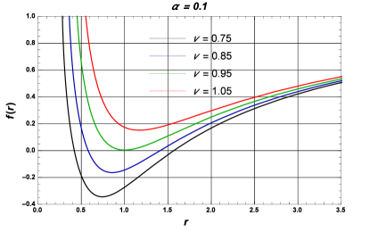
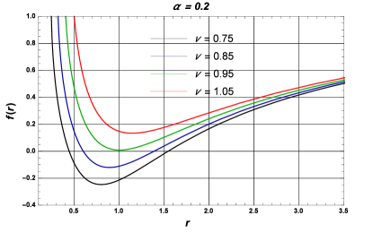
Figure 1: The plots of $f(r)$ vs $r$ for different values of Yang-Mills charge $\nu$ for $-ve$ branch of solution (14) with fixed value of mass $(M=1)$ and ${l=20}$ for different Gauss-Bonnet coupling parameter: $\alpha=0.1$ (left) and $\alpha=0.2$ (right).

	$\alpha=0.1$					$\alpha=0.2$
$\nu$	$r_{-}$	$r_{+}$	$\delta$	$\nu$	$r_{-}$	$r_{+}$	$\delta$
0.75	0.419	1.567	1.146	0.70	0.443	1.543	1.100
0.85	0.579	1.409	0.830	0.80	0.600	1.388	0.788
0.95$(\nu_{c})$	0.995	0.995	0	0.90$(\nu_{c})$	0.995	0.995	0

Table 1: Inner horizon ($r_{-}$), outer horizon ($r_{+}$) and $\delta=r_{+}-r_{-}$ for different values of Yang-Mills charge $\nu$ with fixed value of mass $(M=1)$ and AdS length scale ${l=20}$.

In table 1, we identify the different values of the parameters. Here, $r_{+}$ corresponds to the outer horizon while $r_{-}$ represents the inner horizon. Elementary analysis of the zeros of $f(r)=0$ reveals that it has no zeros if $\nu>\nu_{c}$, one double zero if $\nu=\nu_{c}$, and two simple zeros if $\nu<\nu_{c}$, (Fig. 1). From the figure, it is evident that the two horizons coincide at the critical radius

$$r_{c}=\sqrt{\frac{l^{2}\sqrt{1+\frac{12}{l^{2}}(\alpha+\nu^{2})}-l^{2}}{6}}.$$ (17)

These cases, therefore, describe $4D$ EGB Yang-Mills black hole with degenerate horizon and a non-extreme black hole with both outer and inner Killing horizons, respectively. It is clear that the critical value of $M_{c}$ and $r_{c}$ depend upon the parameters $\alpha$ and $\nu$. Also, the radius of the outer horizon increases with decrease in the Yang-Mills charge $\nu$ and the Gauss-Bonnet coupling $\alpha$ as shown in Fig. 1 and Table 1.

From the standard relation $f(r_{+})=0$, the mass parameter of $4D$ EGB AdS Yang-Mills black hole is calculated as

$$M_{+}=\frac{r_{+}}{2}\left(\frac{r_{+}^{2}+\alpha+\nu^{2}}{r_{+}^{2}}+\frac{r_{+}^{2}}{l^{2}}\right).$$ (18)

From this expression, we can study various thermodynamical quantities of the system.

III Thermodynamics and stability of black hole

In this section, we compute essential thermodynamic quantities which help in checking first-law of thermodynamics and the stability of black holes. In particular we derive Hawking temperature, entropy and heat capacity, chronologically.

The Hawking temperature associated with the black hole is defined in term of horizon radius as following:

$$T_{+}=\frac{\kappa}{2\pi}=\frac{1}{4\pi}f^{\prime}(r)|_{r=r_{+}},$$ (19)

where parameter $\kappa$ refers to the surface gravity.

In our case, the above definition leads to the following value for temperature:

$$T_{+}=\frac{1}{4\pi r_{+}}\left(\frac{r_{+}^{2}-\alpha-\nu^{2}}{r_{+}^{2}+2\alpha}+\frac{3r_{+}^{4}}{l^{2}(r_{+}^{2}+2\alpha)}\right).$$ (20)

For vanishing Yang-Mills charge $\nu=0$, this temperature (20) reduces to the case of the $4D$ AdS EGB black hole,

$$T_{+}=\frac{1}{4\pi r_{+}}\left(\frac{r_{+}^{2}-\alpha}{r_{+}^{2}+2\alpha}+\frac{3r_{+}^{4}}{l^{2}(r_{+}^{2}+2\alpha)}\right).$$ (21)

The relation (20) also reduces to the case of AdS Schwarzschild Yang-Mills black hole and AdS Schwarzschild black hole for $\alpha=0$ and $\nu=0,\alpha=0$, respectively.

Now, in order to study the behaviour of temperature, we plot temperature with respect to event horizon for different values of Yang-Mills charge as shown in Fig. 2.

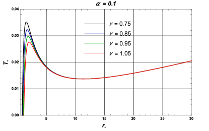
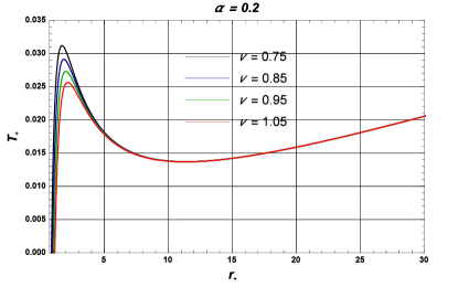
Figure 2: The plot of temperature $T$ vs $r_{+}$ for different values of Yang-Mills charge $\nu$ for Gauss-Bonnet coupling constant $\alpha=0.1$ (left) and $\alpha=0.2$ (right) with fixed value of $l=20$.

From the figure, this is obvious that the Hawking temperature of the $4D$ EGB AdS Yang-Mills black hole grows to a maximum (say $T_{max}$) and then drops to minimum temperature. It turns out that the maximum value of the Hawking temperature decreases with increase of the Yang-Mills charge $\nu$ and Gauss-Bonnet coupling constant $\alpha$. The Hawking temperature vanishes at the critical radius shown in Table 2.

			$\alpha=0.1$					$\alpha=0.2$
$\nu$		0.75	0.85	0.95	1.05		0.75	0.85	0.95	1.05
$r_{c}^{T}$		1.47	1.63	1.82	1.90		1.67	1.77	1.92	2.52
$T_{+}^{Max}$		0.0354	0.323	0.258	0.230		0.0311	0.0290	0.0270	0.256

Table 2: The maximum Hawking temperature ($T_{+}^{max}$) at critical radius ($r_{c}^{T}$) for different values of Yang-Mills charge ($\nu$) with fixed value ${l=20}$.

Now, we calculate another useful quantity associated with the black hole known as entropy $S_{+}$. This black hole can be considered as a thermodynamic system only if the quantities associated with it must obey the first-law of thermodynamics given below

$$dM_{+}=T_{+}dS_{+}+\Phi\,d\nu,$$ (22)

where $\Phi$ is the potential of the black hole. It is matter of calculation only to derive expression of entropy thermo ; Singh:2020xju from the expression (22) at constant $\nu$ as

$$S_{+}=\pi\left(r_{+}^{2}+4\alpha\log[r_{+}]\right).$$ (23)

Finally, we analyse how the background Yang-Mills field affects the thermodynamic stability of the $4D$ EGB AdS black hole by investigating the heat capacity $C_{+}$. The stability of the black hole can be estimated from sign of the heat capacity $C_{+}$ as positive heat capacity reflects the stable black hole and negative reflects the unstable one.

The heat capacity of the black hole can be estimated from the following standard relation cai :

$$C_{+}=\frac{\partial M_{+}}{\partial T_{+}}=\left(\frac{\partial M_{+}}{\partial r_{+}}\right)\left(\frac{\partial r_{+}}{\partial T_{+}}\right).$$ (24)

This leads to

$$C_{+}=\frac{2\pi(r_{+}^{2}+2\alpha)^{2}(3r_{+}^{4}+l^{2}(r_{+}^{2}-\alpha-\nu^{2}))}{3r_{+}^{4}(r_{+}^{2}+6\alpha)-l^{2}(r_{+}^{4}+2\alpha(\alpha+\nu^{2})-r_{+}^{2}(5\alpha+3\nu^{2}))}.$$ (25)

From this expression, it is clearly evident that in the absence of Yang-Mills charge ($\nu$) the heat capacity (25) reduces to

$$C_{+}=\frac{2\pi(r_{+}^{2}+2\alpha)^{2}(3r_{+}^{4}+l^{2}(r_{+}^{2}-\alpha))}{3r_{+}^{4}(r_{+}^{2}+6\alpha)-l^{2}(r_{+}^{4}+2\alpha^{2}-5r_{+}^{2}\alpha)},$$ (26)

which further reduces to the heat capacity of the AdS Schwarzschild black hole in the limit of $\alpha\to 0$. Moreover, Eq. (25) reduces to the heat capacity of the AdS Schwarzschild Yang-Mills black hole when the Gauss-Bonnet coupling switched off ($\alpha\to 0$).

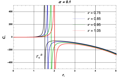
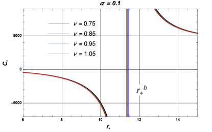
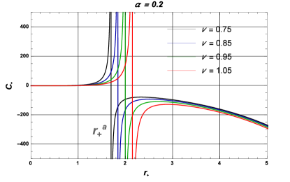
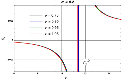
Figure 3: The plot of temperature $T$ vs $r_{+}$ for different values of Yang-Mills charge $\nu$ with fixed value of mass $(M=1)$ and ${l=20}$ for Gauss-Bonnet coupling parameter $\alpha=0.1$ (left) and $\alpha=0.2$ (right).

In order to identify the stability of the heat capacity, we plot expression (25) for different values of Yang-Mills charge $\nu$ and Gauss-Bonnet coupling $\alpha$ as shown in Fig. 3. From the plot, we observe that the heat capacity curve is discontinuous where the temperature is maximum (see Fig. 2 and table 2). The plot clearly shows that the heat capacity diverges at the critical points $r_{+}^{a}$ and $r_{+}^{b}$ with $r_{+}^{a}<r_{+}^{b}$ (see Fig. 3). The $4D$ AdS EGB Yang-Mills black hole is stable for the horizon radius $r_{+}<r_{+}^{a}$ and $r_{+}>r_{+}^{b}$ and unstable for horizon radius $r_{+}^{a}<r_{+}<r_{+}^{b}$. It is obvious from this figure that $4D$ EGB AdS Yang-Mills black hole undergoes phase transition twice firstly at $r_{+}^{a}$ from the stable black hole to the unstable black hole and later at $r_{+}^{b}$ from the unstable black hole ($r_{+}^{a}<r_{+}<r_{+}^{b}$) to stable black hole ($r_{+}>r_{+}^{b}$). Thus, there is a phase transition occurs at $r_{+}=r_{+}^{a}$ and $r_{+}=r_{+}^{b}$ where black hole changes its phase from the stable to unstable phases and vice versa. Further, a divergence of the heat capacity at critical $r_{+}=r_{c}$ signals that this is a second-order phase transition hp ; davis77 .

The heat capacity is discontinuous at $r_{+}=1.47$, at which the Hawking temperature has the maximum value $T_{+}=$ for $\alpha=0.1$ and $\nu=0.75$ (Fig. 3). The phase transition occurs from the higher to lower mass black holes corresponding to positive to negative heat capacity. The critical radius $r_{c}$ increases along with parameter $\alpha$ (cf. Fig. 3 and Table 2).

IV Critical behaviour and phase transition

In the extended phase space the cosmological constant $\Lambda$ is considered as the thermodynamical pressure in order to have Van der Waals like phase transition. The relation between the thermodynamical pressure and cosmological constant is quite standard and given by

$$P=-\frac{\Lambda}{8\pi}=\frac{3}{8\pi l^{2}}.$$ (27)

Here, units are set such that $G=\hbar=c=1$. The pressure and specific volume can be calculated as following:

$$P=\frac{T_{+}(r_{+}^{2}+2\alpha)}{2r_{+}^{3}}-\frac{r_{+}^{2}-\alpha-\nu^{2}}{8\pi r_{+}^{4}},\qquad v=2r_{+}.$$ (28)

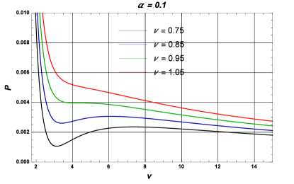
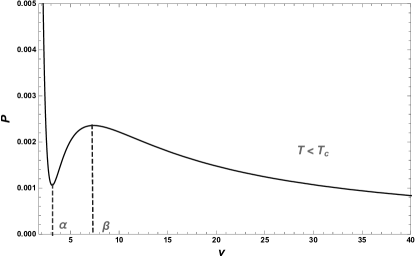
Figure 4: The plot of pressure vs specific volume for $T<T_{c}$, $T=T_{c}$ and $T>T_{c}$ with $T_{c}=0.04038$

In order to study critical behaviour, we plot a $P\--v$ diagram for the $4D$ EGB AdS Yang-Mills black hole as displayed in Fig. 4. Here, we clearly see that a small-large black hole phase transition occurs when the temperature of black hole is less than the critical temperature. To visualize this more clearly, a transition is directly presented on the right panel of Fig. 4. Notice that the $P\--v$ curve contains two stable regions and one unstable region. These stable regions occur for $v\in[0,\alpha]$ and $v\in[\beta,\infty]$ and correspond to the small black hole region and the large black hole region, respectively.

The unstable region $v\in[\alpha,\beta]$ is referred as the spinodal region. In this unstable region, the small and large black hole phase transition can coexist. Furthermore, we note that $\partial P(v,T_{0})/\partial v<0$ for the stable regions, however $\partial P(v,T_{0})/\partial v>0$ for the unstable region.

Mathematically, the two extreme points $\alpha$ and $\beta$ are determined by the relation

$$\left.\frac{\partial P(v,T_{0})}{\partial v}\right|_{\nu=\alpha}=\left.\frac{\partial P(v,T_{0})}{\partial v}\right|_{\nu=\beta}.$$ (29)

Moreover, the inflection point at $\nu=\nu_{0}$ is determined by the relation

$$\left.\frac{\partial^{2}P(v,T_{0})}{\partial v^{2}}\right|_{T}=0.$$ (30)

The critical exponents occur at points of inflections in the $P-v$ diagrams

$$\left.\frac{\partial P_{+}}{\partial r_{+}}\right|_{T}=0,\qquad\qquad\left.\frac{\partial^{2}P_{+}}{\partial r_{+}^{2}}\right|_{T}=0.$$ (31)

This leads to the following values of critical radius, temperature and pressure, respectively rbm ; guna

$$r_{c}=\sqrt{6\alpha+3\nu^{2}+X},$$ (32)

$$T_{c}=\frac{4\alpha+\nu^{2}+X}{2\pi(\sqrt{6\alpha+3\nu^{2}+X})({12\alpha+3\nu^{2}+X})},$$ (33)

$$P_{c}=\frac{52\alpha^{2}+\nu^{2}(9\nu^{2}+49\alpha)+X(3\nu^{2}+7\alpha)}{8\pi({6\alpha+3\nu^{2}+X})^{2}({12\alpha+3\nu^{2}+X})},$$ (34)

where $X=(48\alpha^{2}+48\alpha\nu^{2}+9\nu^{4})^{1/2}.$

These critical values together with relation $v_{c}=2r_{c}$ give the following universal ratio:

$$\rho_{c}=\frac{P_{c}v_{c}}{T_{c}}=\frac{52\alpha^{2}+\nu^{2}(9\nu^{2}+49\alpha)+X(3\nu^{2}+49\alpha)}{2(6\alpha+3\nu^{2}+X)(4\alpha+\nu^{2}+X)}.$$ (35)

In the limit of $\alpha\to 0$ the Eq. (35) resembles to the universal ratio $\rho_{c}=3/8$ rbm . The Universal ratio of the $4D$ AdS EGB black hole $\rho_{c}=0.350$ is slightly smaller than the Van der Waals ratio $\rho_{c}=0.375$ at the small value of $\alpha$ and $\nu$ and the universal ratio increases with increasing values of $\alpha$ and $\nu$ Hegde:2020xlv .

In order to search for the phase structure of the black hole solutions, we derive the free energy in the canonical ensemble. The standard definition for Gibbs free energy reads: $G_{+}=M_{+}-T_{+}S_{+}$ Singh:2020xju . This leads to

$$G_{+} = \frac{3r_{+}^{2}+8\pi Pr_{+}^{4}+3\alpha+3\nu^{2}}{6r_{+}}-\frac{(8\pi Pr_{+}^{4}+r_{+}^{2}-\alpha-\nu^{2})(r_{+}^{2}+4\alpha\log r_{+})}{4r_{+}(r_{+}^{2}+2\alpha)}.$$ (36)

In order to analyse the behaviour of Gibbs free energy, we plot the above expression in terms of temperature. The graph of Gibbs free energy versus temperature for $\alpha=0.1$ and $\alpha=0.2$ with the fixed value of Yang Mills charge $\nu$ is given plotted in Fig. 5.

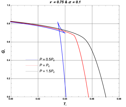
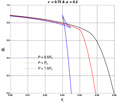
Figure 5: Gibbs free energy vs temperature of $4D$ EGB AdS Yang-Mills black hole for the fixed value of Yang-Mills charge $\nu$. Left: $\alpha=0.1$. Right: $\alpha=0.2$.

The Gibbs free energy which analyses the phase transition of the black holes analogues with the Van der Waals phase transition has the effect of Yang-Mills charge $\nu$ and Gauss-Bonnet coupling constant $\alpha$ on the phase structure of the system. First, we fix the Yang-Mills charge $\nu$ and vary the Gauss-Bonnet coupling constant $\alpha$. The critical pressure and critical temperature increase with critical radius (see Fig. 5) with Yang-Mills charge $\nu$. In $G_{+}-T_{+}$ plots the appearance of characteristic swallow tail shows that the obtained values are critical ones where the phase transition occurs. In Fig. 5, we can see that swallow tail shape exists when $P<P_{c}$ for the first order phase transition and $P=P_{c}$ for the second order phase transition.

V Critical Exponents

In this section, we compute the critical exponent, which is a universal property of phase transition. Usually, near the critical point, a Van der Waals like phase transition is characterized by the four critical exponents $\alpha_{0}$, $\beta$, $\gamma$ and $\delta$ describing the behaviour of the specific heat, order parameter $\eta$, the isothermal compressibility $\kappa_{T}$ and the critical isotherm, respectively. These are defined as

$$C_{v}=T\frac{\partial S}{\partial T}\propto|\tau|^{-\alpha_{0}},\qquad\qquad\eta=v_{l}-v_{s}\propto|\tau|^{\beta},$$ (37)

$$\kappa_{T}=-\frac{1}{v}\frac{\partial v}{\partial p}\propto|\tau|^{-\gamma},\quad\qquad|P-P_{c}|_{T_{c}}\propto|v-v_{c}|^{\delta},$$ (38)

where $\tau=\frac{T-T_{c}}{T_{c}}$ and $v_{l}$ and $v_{s}$ denote specific volume of large and small black holes, respectively.

Now, with the following definitions:

$$p=\frac{P}{P_{c}},\qquad\qquad t=\frac{T}{T_{c}}=\tau+1,\qquad\text{and}\qquad\lambda=\frac{v}{v_{c}},$$ (39)

the equation of state translate into so-called law of corresponding states and reads

$$\frac{8p}{3}=\frac{t}{\lambda}-\frac{t\alpha_{0}}{6\lambda^{3}}-\frac{}{}\left(\frac{1}{\lambda}+\frac{2\alpha_{0}}{\lambda}+\frac{2\nu^{2}}{36\lambda^{4}}\right).$$ (40)

Let us calculate the critical exponents predicted by the corresponding states (40). We define

$$\qquad\qquad\omega=\frac{v-v_{c}}{v_{c}}=\lambda-1.$$ (41)

To find the critical exponents we expend equation of state near the critical points as following:

$$p=1+a_{10}\tau-a_{11}\tau\omega-a_{30}\omega^{3}+{\cal O}(\tau\omega^{2},\omega^{4}),$$ (42)

In the absence of Gauss-Bonnet coefficient, the above coefficients resemble to the Reissner-Nordström black hole. Differentiating the Eq. (42) with respect to $\omega$ for fixed value of $t$, we get

$$dP=P_{c}\left(a_{11}\tau+a_{30}\omega^{2}\right)d\omega.$$ (43)

If the black hole undergoes the phase transition from small to large one keeping temperature and pressure constant while changing the thermodynamic volume from $\omega_{s}$ to $\omega_{l}$, the equation of state always holds, i.e.,

$$p=1+a_{10}\tau-a_{11}\tau\omega_{l}-a_{30}\omega_{l}^{3}=1+a_{10}\tau-a_{11}\tau\omega_{s}-a_{30}\omega_{s}^{3}.$$ (44)

Moreover, during the phase transition, the Maxwell’s area law also holds, i.e.,

$$\int_{\omega_{l}}^{\omega_{s}}\omega dP=\omega\left(a_{11}\tau+a_{30}\omega^{2}\right)dP=0.$$ (45)

Solving for the above equations, we obtain a non-trivial solution

$$\omega_{l}=-\omega_{s}=\sqrt{-\frac{a_{11}\tau}{a_{30}}}=2\sqrt{-\tau}.$$ (46)

Hence we have the order parameter $\eta$ as

$$\eta=v_{c}(\omega_{l}-\omega_{s})=\sqrt{-\frac{a_{11}\tau}{a_{30}}}\propto\sqrt{-t}=4v_{c}\sqrt{-\tau}.$$ (47)

The relations (37) and (47) confirm that $\beta=1/2$.

The isothermal compressibility $\gamma$ is calculated by

$$\kappa_{T}=-\left.\frac{1}{P_{c}(1+\omega)}\frac{\partial\omega}{\partial P}\right|_{T}\propto\frac{1}{6P_{c}}\frac{1}{\tau}.$$ (48)

This implies that $\gamma=1$.

The critical isotherm at $\tau=0$ is estimated from Eq. (42) as $\delta=3$ as $p-1=-\frac{4}{81}(1-\alpha_{0})\omega^{3}$. Consequently, the four critical exponents are identified as

$$\alpha_{0}=0,\qquad\beta=\frac{1}{2},\qquad\gamma=1\qquad\text{and}\qquad\delta=3.$$ (49)

Obviously the entropy is not dependent of temperature and hence the critical exponent $\alpha_{0}=0$. These critical exponents resembles to the Van der Walls fluid and these critical exponents satisfy the following thermodynamics scaling laws

$$\alpha_{0}+2\beta+\gamma=2,\qquad\alpha_{0}+\beta(\delta+1)=2,\qquad(1-\alpha_{0})\delta=1+(2-\alpha_{0}),$$ (50)

$$\gamma(\delta+1)=(2-\alpha_{0})(\delta-1)\qquad\text{and}\qquad\gamma=\beta(\delta-1).$$ (51)

We conclude that the thermodynamics exponents associated with the AdS EGB black hole with Yang-Mills field in the extended phase agree with the mean field theory prediction rbm ; guna ; lala .

Charged (Abelian) black hole solution with some thermal properties have been studied so far for the $4D$ AdS EGB model fran ; Singh:2020xju ; Hegde:2020xlv . Here, we have generalized the black hole solution for $4D$ AdS EGB gravity model in presence of Yang-Mills (non-Abelian) charge. In fact, we explore the critical behaviour, phase transition and the critical exponents also along with thermodynamics of the model. With an appropriate limiting case, one can recover the solutions of aforementioned references.

VI Discussions and Conclusions

We have found an exact solution for $4D$ EGB black hole in the presence of Yang-Mills field which is a generalization of the solution obtained by Glavan and Lin gla . Also, one recovers the Schwarzschild AdS solution for $\alpha\rightarrow 0$, $\nu\rightarrow 0$ and $l\rightarrow\infty$. Furthermore, we have investigated the thermodynamics behaviour of the solution. Here, we have observed that the thermodynamics quantities get modification due to the presence of Yang-Mills charge $\nu$. However, the entropy of the black hole remains unaffected by the Yang-Mills charge and turns out to be the Bekenstein-Hawking area-law for the novel $4D$ EGB black hole. In order to discuss the stability of the black hole we derive the heat capacity. The heat capacity $C_{+}$ diverges at a critical radius $r=r_{c}$, where the temperature has a maximum and $C_{+}>0$ for $r_{+}<r_{c}$ allowing the black hole to become thermodynamically stable.

We also examined the $P\--v$ criticality and phase structure of the $4D$ AdS EGB black hole solution with Yang-Mills charge. We have found that a small-large black hole phase transition occurs for the case where temperature is less than the critical temperature, i.e., $T<T_{c}$. The critical exponents are also calculated which increase with the Yang-Mills charge $\nu$ and decrease with the GB coupling constant $\alpha$. It will be interesting to study the effect of thermal and geometric fluctuation on the thermodynamics of this black hole solution. This is the subject of future investigation.

Appendix A The equations of motion for EGB gravity with Yang-Mills field

The action of the $D$-dimensional EGB gravity in the presence of Yang-Mills field is given by

$$S = \frac{1}{2}\int d^{D}x\sqrt{-g}\left[{\cal R}-2\Lambda+\frac{\alpha}{D-4}{\cal L_{GB}}-{\cal F}_{YM}\right],$$ (52)

where $\mathcal{L_{GB}}$ is Lagrangian density for EGB gravity and has following expression:

$$\mathcal{L_{GB}}={\cal R}_{\mu\nu\gamma\delta}{\cal R}^{\mu\nu\gamma\delta}-4{\cal R}_{\mu\nu}{\cal R}^{\mu\nu}+{\cal R}^{2}.$$

The equation of motion for metric tensor $g_{\mu\nu}$ and the electromagnetic potential ${\cal A}_{\mu}^{(a)}$ are given, respectively, by

$$G_{\mu\nu}+\Lambda g_{\mu\nu}+H_{\mu\nu}=T_{\mu\nu}^{YM},$$ (53)

$$D_{\mu}F^{(a)\mu\nu}=0,$$ (54)

where

$$G_{\mu\nu} = {\cal R}_{\mu\nu}-\frac{1}{2}g_{\mu\nu}{\cal R},$$ (55)

$$H_{\mu\nu} = -\frac{\alpha}{2}\left[8{\cal R}^{\rho\sigma}{\cal R}_{\mu\rho\nu\sigma}-4{\cal R}_{\mu}^{\rho\sigma\lambda}{\cal R}_{\nu\rho\sigma\lambda}-4{\cal R}{\cal R}_{\mu\nu}+8{\cal R}_{\mu\lambda}{\cal R}_{\nu}^{\lambda}\right.$$

$$+ \,\,\left.g_{\mu\nu}\left({\cal R}_{\rho\sigma\gamma\delta}{\cal R}^{\rho\sigma\gamma\delta}-4{\cal R}_{\rho\sigma}{\cal R}^{\rho\sigma}+{\cal R}^{2}\right)\right],$$

$$T_{\mu\nu}^{YM} = -\frac{1}{2}g_{\mu\nu}F_{\rho\sigma}^{(a)}F^{(a)\rho\sigma}+2F_{\mu\sigma}^{(a)}F^{(a)\sigma}_{\ \nu}.$$ (56)

Here ${\cal R}$, ${\cal R}_{\mu\nu}$ and ${\cal R}_{\mu\nu\gamma\delta}$ the $D=d+1$ dimensional Ricci scalar, Ricci tensor and Riemann tensor, respectively.

References

- (1) D. Lovelock, J. Math. Phys. 12 (1971) 498.
- (2) B. Zwiebach, Phys. Lett. B 156 (1985) 315.
- (3) S. H. Hendi, B. Eslam Panah and S. Panahiyan, JHEP 11 (2015) 157.
- (4) S. Upadhyay, Gen. Rel. Grav. 50 (2018) 128.
- (5) S. Upadhyay, S. H. Hendi, S. Panahiyan and B. E. Panah, Prog. Theor. Exp. Phys. 093E01 (2018) 1.
- (6) B. Pourhassan, S. Upadhyay, H. Saadat and H. Farahani, Nucl. Phys. B928 (2018) 415.
- (7) S. Upadhyay, Phys. Lett. B775 (2018) 130.
- (8) S. Hawking and D. N. Page, Commun. Math. Phys. 87 (1983) 577.
- (9) X. O. Camanho, J. D. Edelstein, G. Giribet and A. Gomberoff, Phys. Rev. D 90 (2014) 064028.
- (10) X. O. Camanho, J. D. Edelstein, A. Gomberoff and J. A. Sierra-Garcia, JHEP 10 (2015) 179.
- (11) X. O. Camanho, J. D. Edelstein, G. Giribet and A. Gomberoff, Phys. Rev. D 86 (2012) 124048.
- (12) D. Kubiznak and R.B. Mann, JHEP 07 (2012) 033.
- (13) S. Gunasekaran, R.B. Mann and D. Kubiznak, JHEP 11 (2012) 110.
- (14) N. Altamirano,D. Kubiznak, R.B. Mann and Z. Sherkatghanad, Class. Quant. Grav. 31 (2014) 042001.
- (15) R. A. Hennigar, W. G. Brenna and R. B. Mann, JHEP 07 (2015) 077.
- (16) R. A. Hennigar, D. Kubiznak and R. B. Mann, Phys. Rev. Lett. 115 (2015) 031101.
- (17) R. A. Hennigar and R. B. Mann, Entropy 17 (2015) 8056.
- (18) D. Glavan and C. Lin, Phys. Rev. Lett. 124 (2020) 081301.
- (19) K. Aolki, M. A. Gorji and S. Mukohyama, Phys. Lett. B 810 (2020) 135843.
- (20) K. Aolki, M. A. Gorji and S. Mukohyama, JCAP 2009 (2020) 014.
- (21) P. G. S. Fernandes, Phys. Lett. B 805 (2020) 135468.
- (22) D. V. Singh, S. G. Ghosh and S. D. Maharaj, Phys. Dark Univ. 30 (2020) 100730.
- (23) R. A. Hennigar, D. Kubizňák, R. B. Mann and C. Pollack, JHEP 07 (2020) 027.
- (24) A. Kumar and R. Kumar, arXiv:2003.13104.
- (25) R. A. Konoplya and A. F. Zinhailo, arXiv:2003.01188.
- (26) M. Guo and P. C. Li, arXiv:2003.02523.
- (27) A. Casalino, A. Colleaux, M. Rinaldi and S. Vicentini, arXiv:2003.07068.
- (28) S.-W. Wei and Y.-X. Liu, arXiv:2003.07769.
- (29) R. A. Konoplya and A. Zhidenko, arXiv:2003.07788.
- (30) S. G. Ghosh, D. V. Singh, R. Kumar and S. D. Maharaj, Annals Phys. 424 (2021), 168347.
- (31) K. Yang, B. M. Gu, S. W. Wei and Y. X. Liu, Eur. Phys. J. C 80 (2020) 662.
- (32) S. Devi, R. Roy and S. Chakrabarti, Eur. Phys. J. C 80 (2020) 760.
- (33) A. K. Mishra, Gen. Rel. Grav. 52 (2020) 106.
- (34) X. H. Jin, Y. X. Gao and D. J. Liu, Int. J. Mod. Phys. D 29 (2020) 2050065.
- (35) S. U. Islam, R. Kumar and S. G. Ghosh, JCAP 09 (2020) 030.
- (36) R. A. Konoplya and A. F. Zinhailo, Phys. Lett. B 810 (2020) 135793.
- (37) S. W. Wei and Y. X. Liu, Phys. Rev. D 101 (2020) 104018.
- (38) D. V. Singh and S. Siwach, Phys. Lett. B 808 (2020) 135658.
- (39) C. M. Zhang, D. C. Zou and M. Zhang, Phys. Lett. B 811 (2020) 135955.
- (40) B. K. Singh, R. P. Singh and D. V. Singh, Eur. Phys. J. Plus 136 (2021) 575.
- (41) B. K. Singh, R. P. Singh and D. V. Singh, Eur. Phys. J. Plus 135 (2020) 862.
- (42) S. H. Hendi, M. Momennia, JHEP 10 (2019) 207.
- (43) B. Eslam Panah, Kh. Jafarzade, S. H. Hendi, Nucl. Phys. B 961 (2020) 115269.
- (44) S. H. Hendi, M. Momennia, Phys. Lett. B 777 (2018) 222.
- (45) S. H. Hendi, B. Eslam Panah, S. Panahiyan, M. S. Talezadeh, Eur. Phys. J. C 77 (2017) 133.
- (46) S. H. Hendi, B. Eslam Panah, S. Panahiyan Class. Quant. Grav. 33 (2016) 235007.
- (47) S. H. Hendi, S. Panahiyan, Phys. Rev. D 90 (2014) 124008.
- (48) S. H. Hendi, B. E. Panah and S. Panahiyan, Fortsch. Phys. 66 (2018) 1800005.
- (49) A. B. Balakin, J. P. S. Lemos and A. E. Zayats, Phys. Rev. D 93 (2016) 024008.
- (50) J. M. Bardeen, B. Carter, and S.W. Hawking, Commun. Math. Phys. 31 (1973) 161-170.
- (51) R. G. Cai, Phys. Rev. D 65 (2002) 084014.
- (52) S. Hawking and D. Page, Commun. Math. Phys. 87 (1983) 577.
- (53) P. Davis, Proc. R. Soc. A 353 (1977) 499.
- (54) S. Gunaseharan, D. Kubiznak and R. B. Mann, JHEP 11 (2012) 033.
- (55) D. Kubiznak and R. B. Mann, JHEP 07 (2012) 110.
- (56) K. Hegde, A. Naveena Kumara, C. L. A. Rizwan, A. K. M. and M. S. Ali, arXiv:2003.08778.
- (57) A. Lala, Advances in High Energy Physics 2013 (2013) 1 [arXiv:1205.6121].