Role of limiting dispersal on metacommunity stability and persistence

Abstract

The role of dispersal on the stability and synchrony of a metacommunity is a topic of considerable interest in theoretical ecology. Dispersal is known to promote both synchrony, which enhances the likelihood of extinction, and spatial heterogeneity, which favours the persistence of the population. Several efforts have been made to understand the effect of diverse variants of dispersal in the spatially distributed ecological community. Despite the environmental change strongly affect the dispersal, the effects of controlled dispersal on the metacommunity stability and their persistence remain unknown. We study the influence of limiting the immigration using two patch prey-predator metacommunity at both local and spatial scales. We find that the spread of the inhomogeneous stable steady states (asynchronous states) decreases monotonically upon limiting the predator dispersal. Nevertheless, at the local scale, the spread of the inhomogeneous steady states increases up to a critical value of the limiting factor, favoring the metacommunity persistence, and then starts decreasing for further decrease in the limiting factor with varying local interaction. Interestingly, limiting the prey dispersal promotes inhomogeneous steady states in a large region of the parameter space, thereby increasing the metacommunity persistence both at spatial and local scales. Further, we show similar qualitative dynamics in an entire class of complex networks consisting of a large number of patches. We also deduce various bifurcation curves and stability condition for the inhomogeneous steady states, which we find to agree well with the simulation results. Thus, our findings on the effect of the limiting dispersal can help to develop conservation measures for ecological community.

I Introduction

Synchrony, referring the coherent behaviour of coupled systems Pikovsky et al. (2001), has been studied extensively in numerous fields such as neuroscience, physiology, biology, ecology Izhikevich (2007); Blasius et al. (1999); Liebhold et al. (2004), etc. In population dynamics, synchrony has received a great deal of attention since it can elevate a high risk of extinction Ranta et al. (1995); Liebhold et al. (2004); Briggs and Hoopes (2004); Goldwyn and Hastings (2008). Indeed, understanding the factors and mechanisms that generate population synchrony in ecology is of great importance for conservation and ecosystem management. Three major mechanisms of population synchrony are dispersal, environmental variation and trophic interactions Ranta et al. (1997); Kendall et al. (2000); Liebhold et al. (2004). Among these, dispersal is a widely studied phenomenon in population dynamics Heino et al. (1997); Blasius et al. (1999); Goldwyn and Hastings (2008); Holland and Hastings (2008). Interestingly, dispersal not only leads to synchronized behaviour among the spatially distributed populations, but it can also rescue populations through recolonization Doebeli (1995); Hanski (1998, 1999). Consequently, dispersal can also act as a stabilizing mechanism in diverse systems and has a huge impact on the persistence of ecological communities Briggs and Hoopes (2004); Wang and Loreau (2016). In this scenario, a small change or a control over the dispersal can have tremendous consequences on the stability and ecosystem functioning. In this study, we present how limiting the dispersal of both predator and prey populations can affect the stability and persistence of a spatially distributed community.

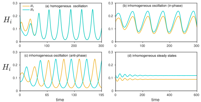
Figure 1: Homogeneous and inhomogeneous stable states of the metacommunity model: (a) homogeneous oscillatory state for $d_{h}=0.2$ and $k=0.2$, (b) inhomogeneous oscillatory states are in in-phase for $d_{h}=1$ and $k=1.2$, (c) inhomogeneous stable oscillatory states are in anti-phase for $d_{h}=0.001$ and $k=0.6$, and (d) inhomogeneous steady states for $d_{h}=0.45$ and $k=0.6$. Other parameters are $r=0.5$, $a=1$, $c=0.5$, $b=0.16$, $m=0.2$, $d_{v}=0.001$ and $\alpha=\beta=1$.

Climate change affects the stability of many ecological communities by altering their dispersal pattern and the associated responses McPeek and Holt (1992); Doebeli and Ruxton (1997); Travis et al. (2013); Fussmann et al. (2014). Major ecological responses to environmental changes include adaptation, migration and extinction Walther et al. (2002); Parmesan (2006); Berg et al. (2010); Walther (2010); Reed et al. (2011). Species that lacks the adaptation for environmental variation tends to migration to suitable habitats. While species migrate, it can face an additional mortality due to failed migration, misdirected migration and also overcrowding Mueller et al. (2013). Typically, species immigration is reduced by habitat loss, habitat fragmentation and anthropogenic changes Walther et al. (2002); Parmesan (2006); Püttker et al. (2011). Indeed, climate change and other factors can also limit the species dispersal. In this connection, theoretical studies addressing the effect of controlled dispersal is extremely rare. Despite a plethora of studies focused on understanding the role of dispersal on the metacommunity persistence, it remains unclear how a limited dispersal affects the metacommunity stability. Since coupled ecological oscillators constitute an efficient framework to understand the dynamical effects of dispersal, in this work, we address (i) how a limited dispersal of both predator and prey populations affects the stability and persistence of a spatially distributed community, and (ii) how limited dispersal along with local and spatial interactions influences the synchronized and asynchronized dynamics of the metacommunity?

In this study, we address the dynamical effects of limiting the dispersal of a predator-prey ecological system. In particular, we investigate the metacommunity persistence using homogeneous (synchronized) and inhomogeneous (asynchronized) dynamical behaviour by limiting the predator and prey dispersal. Our results reveal that a small change in the predator dispersal monotonically reduces the inhomogeneous behaviour as a function of the spatial interaction (predator/prey dispersal rates). In contrast, for a varying local interaction (carrying capacity), a small decrease in the predator dispersal initially increases the inhomogeneous states up to a critical value of the limiting factor and eventually the inhomogeneous states lose its stability resulting in homogeneous dynamical state for further decrease in the degree of the limited dispersal. Moreover, there exists a critical value of the limiting factor below which the metacommunity persists and above which metacommunity has a risk of extinction. On the other hand, limiting the prey dispersal manifests the stable inhomogeneous steady states in a large region of the parameter space, thereby increasing the metacommunity persistence. We also consider an entire class of complex networks of metacommunity to corroborate robustness of the results. We also deduce transcritical and Hopf bifurcation curves along with stability condition for the inhomogeneous steady state for a possible case. We find that the stability condition agrees well with the simulation results. This study unveils that a controlled dispersal strongly influence the metacommunity persistence by altering the asynchronized dynamics.

We organize the paper in the following order. In the ‘Models and methods’ section, we describe a two-patch predator-prey metacommunity model with limiting factors in the diffusive coupling. In the ‘Results’ section, we present the effect of limited predator and prey dispersal using local and spatial interactions. We also deduce the stability condition for the inhomogeneous steady (asynchronized alternative) states for the possible scenario. Subsequently, we elucidate the existence of a critical value of the limited dispersal influencing the synchronized behaviour. Further, we extend our analysis to the entire class of complex networks of metacommunity to generalize our results. Finally, we discuss the ecological significance of our findings in the ‘Discussion’ section.

II Models and methods

II.1 A metacommunity model

We use the well-known Rosenzweig-MacArthur model Rosenzweig and MacArthur (1963) to represent the prey-predator dynamics in each patch, where prey experiences logistic growth and predator exhibits a Holling Type II functional response. We consider two identical patches with diffusive coupling between them, whose governing equation is represented as

$$\frac{dV_{i}}{dt} =rV_{i}\left(1-\frac{V_{i}}{k}\right)-\frac{aV_{i}}{V_{i}+b}H_{i}+d_{v}(\beta V_{j}-V_{i})\;,$$ (1a)

$$\frac{dH_{i}}{dt} =\frac{caV_{i}}{V_{i}+b}H_{i}-mH_{i}+d_{h}(\alpha H_{j}-H_{i})\;,$$ (1b)

where $i,j=1,2$ denote the patch number and $i\neq j$. $V_{i}$ and $H_{i}$ are the prey and predator population densities, respectively. The parameter $r$ denotes the intrinsic growth rate, $k$ denotes the carrying capacity, $a$ and $c$ denote the maximum predation rate and predator efficiency, respectively. Half-saturation constant is denoted by $b$ and the mortality rate of the predator by $m$. These parameters determine the local dynamics of the prey and the predator in a given patch. The spatial interactions of the prey and predator between two patches are determined by the prey dispersal rate $d_{v}$, predator dispersal rate $d_{h}$ and the limiting factors $\alpha$ and $\beta$. Dispersal between the patches is controlled by the limiting factors, which can be decreased from $1$ to zero. For $\alpha=\beta=1$, the coupling is the usual diffusive coupling widely employed in the population ecology Goldwyn and Hastings (2008); Holland and Hastings (2008). $\alpha<1$ accounts for the limited predator dispersal by reducing the immigration of the predator from patch $j$ to patch $i$, while $\beta<1$ accounts for the limited prey dispersal by reducing the immigration of the prey from patch $j$ to patch $i$.

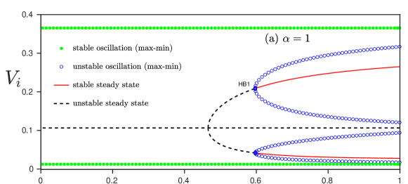
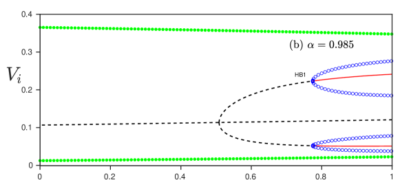
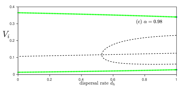
Figure 2: Metacommunity dynamics for limiting the predator dispersal: Bifurcation diagram as a function of predator dispersal rate ($d_{h}$) is shown for different $\alpha$ values. Homogeneous and inhomogeneous states of the metacommunity are shown for (a) $\alpha=1$, (b) $\alpha=0.985$, and (c) $\alpha=0.98$. For a small decrease in $\alpha$, inhomogeneous stable steady states (red solid lines) become unstable. Here HB1 denotes Hopf bifurcation. Other parameters are $\beta=1$, $r=0.5$, $k=0.5$, $a=1$, $c=0.5$, $b=0.16$, $m=0.2$ and $d_{v}=0.001$.

Note that the coupled Rosenzweig-MacArthur model with $\alpha=\beta=1$ has been widely employed to understand the intriguing collective dynamical behaviours under various coupling scenarios Dutta and Banerjee (2015); Arumugam et al. (2016); Arumugam and Dutta (2018); Arumugam et al. (2021). In particular, the coexistence of spatially synchronized state and death state, leading to chimeralike state, has been reported in nonlocally coupled Rosenzweig-MacArthur model Dutta and Banerjee (2015), the phenomenon of rhythmogenesis including amplitude and oscillation deaths has been reported under the environmental coupling Arumugam et al. (2016), the effect of trade-off between the mismatch in the timescale of the species, dispersal and external force on the collective dynamics has been reported in diffusively coupled Rosenzweig-MacArthur model Arumugam and Dutta (2018) and the effect of prey-predator dispersal on the metacommunity persistence in both constant and temporally varying environment has been reported in spatially coupled Rosenzweig-MacArthur models Arumugam et al. (2021).

II.2 Rescaled version of coupled Rosenzweig-MacArthur model

The above two coupled Rosenzweig-MacArthur model with $\alpha$ and $\beta$ limiting predator and prey dispersal rates, respectively, can also be written as a rescaled model with standard diffusive coupling represented as

$$\frac{dV_{i}}{dt} =r_{e}V_{i}\left(1-\frac{V_{i}}{k_{e}}\right)-\frac{aV_{i}}{V_{i}+b}H_{i}+\epsilon_{v}(V_{j}-V_{i})\;,$$ (2a)

$$\frac{dH_{i}}{dt} =\frac{caV_{i}}{V_{i}+b}H_{i}-m_{e}H_{i}+\epsilon_{h}(H_{j}-H_{i})\;,$$ (2b)

where, $r_{e}=r-d_{v}(1-\beta),k_{e}=\frac{r_{e}}{r}k=1-\frac{d_{v}}{r}(1-\beta),\epsilon_{v}=d_{v}\beta,m_{e}=m+d_{h}(1-\alpha)$ and $\epsilon_{h}=d_{h}\alpha$. Here, $r_{e}$ is the decreased growth rate, $m_{e}$ is the increased mortality, $k_{e}$ is the effective carrying capacity, and $\epsilon_{v}$ and $\epsilon_{h}$ are the rescaled coupling coefficients. Since the range of $\beta$ and $\alpha$ lies within $[1,0]$, $r_{e}\leq r$ and $m_{e}\geq m$ resulting in decreased prey growth rate and increased predator death rate in the rescaled version of coupled Rosenzweig-MacArthur model. Note that the results of both the rescaled model with standard diffusive coupling and the original Rosenweig-MacAurther model with limiting predator and prey dispersal rates in the coupling will be exactly similar to each other. In other words, the exact mapping between these two models can also be interpreted as that the observed results may not a pure manifestation of the topological features. However, we prefer to proceed our analysis without rescaling the original Rosenweig-MacAurther model but only by engineering the coupling strategies even though limiting the predator and prey dispersal rates effectively results in an increase in the predator’s death rate $m_{e}$ and decrease in the prey growth rate $r_{e}$, respectively.

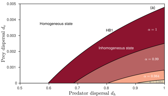
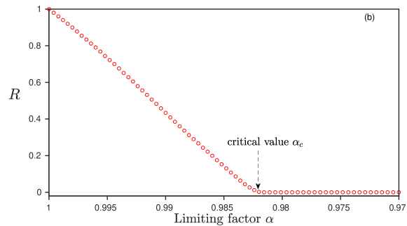
Figure 3: (a) Two parameter bifurcation diagram in $d_{h}-d_{v}$ space at different $\alpha$ values: Hopf bifurcation (HB1) curve separates the region into homogeneous and inhomogeneous stable states. The region below the curve indicates the spread of the inhomogeneous stable states that decreases for decreasing $\alpha$. (b) The normalized area of the spread of the stable inhomogeneous steady states defined as $R=S(\alpha)/S(\alpha=1)$, where $S(\alpha)$ denotes the spread of the stable inhomogeneous steady states for $\alpha$. Other parameter values are $\beta=1$, $r=0.5$, $k=0.5$, $a=1$, $c=0.5$, $b=0.16$ and $m=0.2$.

III Results

Before unravelling the effect of limited dispersal, we illustrate various dynamical states admitted by the metacommunity model for distinct values of the system parameters in Fig. 1. The limiting factors are fixed as $\alpha=\beta=1$, so that the coupling is the regular diffusive coupling, which accounts for the uncontrolled dispersal Arumugam et al. (2021). We numerically integrate the governing equation of the metacommunity model using the Runge-Kutta 4th order algorithm with a step size of $h=0.01$. We have fixed the other parameters as $r=0.5$, $a=1$, $c=0.5$, $b=0.16$, $m=0.2$, and $d_{v}=0.001$ throughout the manuscript unless otherwise specified. Note that we have chosen the model parameters in order to get oscillatory dynamics in the uncoupled model. Indeed, the uncoupled predator-prey model exhibits the oscillatory dynamics when

$$k>\frac{b\left[ac+m+(1-\alpha)d_{h}\right]}{ac+(\alpha-1)d_{h}-m}.$$

The model (1) exhibits similar qualitative dynamics even for other choice of the parameters. Homogeneous oscillatory state is observed for the predator dispersal rate $d_{h}=0.2$ and for the carry capacity $k=0.2$ as depicted in Fig. 1(a), which has a high probability of extinction under environmental stochasticity during the epochs of low population density. Phase synchrony (inhomogeneous oscillatory states) can be observed for $d_{h}=1.0$ and $k=1.2$ (see Fig. 1(b)), which is also prone to global extinction like the homogeneous oscillatory state in Fig. 1(a), but with a lesser probability when compared to the latter at low population density. Anti-phase synchronization (inhomogeneous oscillatory states) can be observed in Fig. 1(c) for $d_{h}=0.001$ and $k=0.6$, which has a much lesser chance of extinction when compared to the homogeneous and phase synchronized populations. One can also observe inhomogeneous steady states (see Fig. 1(d) for $d_{h}=0.45$ and $k=0.6$) of the populations, which usually coexist with homogeneous (synchronized) oscillatory state, resulting in alternative dynamical states for the population to promote their persistence.

III.1 limiting predator dispersal along with spatial interaction

In this section, we will unravel the effect of limiting the predator dispersal on the dynamical transitions of the metacommunity model as a function of spatial parameters (predator and prey dispersal rates). We fix $\beta=1$, so that the preys are allowed to disperse completely, whereas only the predator dispersal is controlled by decreasing the value of $\alpha$. Bifurcation diagrams, plotted using XPPAUT  Ermentrout (2002), illustrating the dynamical transitions as a function of the predator dispersal rate are depicted in Fig. 2 for the carrying capacity $k=0.5$. Extrema of stable homogeneous oscillatory state are plotted as filled circles, while that of unstable oscillatory states are represented by unfilled circles. Stable and unstable steady states are indicated by solid and dashed curves/lines, respectively. For $\alpha=1$, the dispersal among the metacommunity is the usual diffusive coupling between the patches. Only stable homogeneous (synchronized) oscillation among the populations is observed all along the low values of the predatory dispersal for $\alpha=1$, where the homogeneous steady state is unstable (see Fig. 2(a)). The former prevails in the entire explored range of the predator dispersal rate. Subcritical pitchfork bifurcation onsets at $d_{h}=0.48$ resulting in the coexistence of unstable homogeneous and inhomogeneous steady states along with the homogeneous oscillatory state in the range of $d_{h}\in[0.48,0.597)$. A Hopf bifurcation at $d_{h}=0.597$ leads to the onset of stable inhomogeneous steady (asynchronous) states, which coexist along with unstable inhomogeneous oscillatory states. The onset of the former gives rise to the emergence of alternative stable states of the populations thereby leading to an increase in the degree of persistence of the metacommunity in the range of $d_{h}\in[0.597,1.0]$.

Now, we control the dispersal rate of the predators using the limiting factor $\alpha$ and investigate the effect of limited dispersal on the metacommunity persistence. The dynamical transitions of the prey density are depicted in Fig. 2(b) for $\alpha=0.985$. It is evident from the figure that even a feeble decrease in the limiting factor, that is a negligible fraction of decrease in dispersal, results in drastic changes in the metacommunity dynamics. The Hopf bifurcation, resulted in the onset of alternative stable states, now emerges at a higher dispersal rate at $d_{h}=0.7745$ reducing the tolerance of the metacommunity persistence to a narrow range of predator dispersal rate. This effect of limiting dispersal increases to a larger degree for further negligible decrease in the fraction of dispersal. As a consequence, the alternative stable states lose its stability in the explored range of $d_{h}$ even for $\alpha=0.98$, denoting a very small decrease in the degree of the dispersal, endangering the persistence of the metacommunity due to the presence of the homogeneous (synchronous) oscillatory state as the only dynamical state of the metacommunity, which is highly prone to extinction. In the following, we will explore the effect of controlling the predator dispersal on the metacommunity dynamics as a function of the dispersal rate of both prey and predator populations.

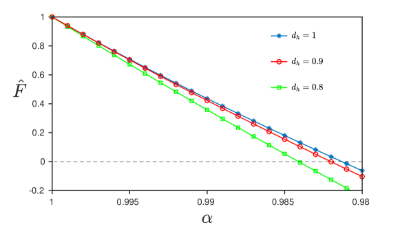
Figure 4: Analytical stability curve for different predator dispersal rates. The values of the parameters are the same as in Fig. 3.

We have depicted the spread of the inhomogeneous steady (asynchronous, alternative) states in the two-parameter bifurcation diagram in Fig. 3(a) for different degree of the dispersal by reducing the limiting factor $\alpha$. Homogeneous oscillatory state is stable in the entire parameter space, while the inhomogeneous steady states are stable in the shaded region, where both the former and the latter coexists. The transition from homogeneous to inhomogeneous steady state is via the Hopf bifurcation as depicted in one parameter bifurcation diagrams in Fig. 2. Note that the Hopf bifurcation curves are obtained from XPPAUT. The spread of the inhomogeneous steady states is maximum for $\alpha=1$, which monotonically decreases for further decrease in the degree of the predator dispersal. Eventually, the inhomogeneous steady states destabilized completely in the same parameter space, where it was stable earlier, at a critical value of $\alpha$ resulting in the homogeneous (synchronous) oscillatory state as the only dynamical state of the metacommunity. The normalized area of the spread of the stable inhomogeneous steady states defined as $R=S(\alpha)/S(\alpha=1)$, where $S(\alpha)$ denotes the spread of the stable inhomogeneous steady states for $\alpha$, is depicted in Fig. 3(b) as a function of $\alpha$. It is evident from the figure that the spread of the stable inhomogeneous steady states decreases monotonically and eventually vanishes at the critical value of $\alpha=\alpha_{c}\approx 0.9818$ corroborating the dynamical transitions observed in the one- and two-parameter bifurcation diagrams.

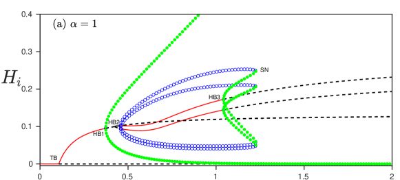
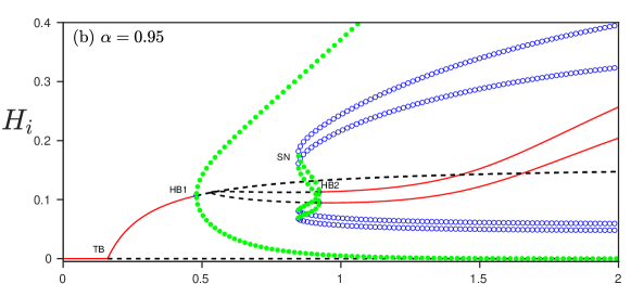
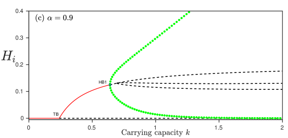
Figure 5: Metacommunity dynamics for limiting the predator dispersal: Bifurcation diagram as a function of the carrying capacity ($k$) is shown for different $\alpha$ values. Homogeneous and inhomogeneous states of the metacommunity are shown for (a) $\alpha=1$, (b) $\alpha=0.95$, and (c) $\alpha=0.9$. For a decrease in $\alpha$, inhomogeneous stable steady states (red solid lines) becomes unstable. Here TB, HB and SN correspond to transcritical bifurcation, Hopf bifurcation and saddle-node bifurcation, respectively. Other parameters are $r=0.5$, $a=1$, $c=0.5$, $b=0.16$, $m=0.2$, $d_{v}=0.001$ and $d_{h}=1$.

It is extremely difficult to extract the inhomogeneous steady states and deduce its stability condition analytically for finite values of prey dispersal rate $d_{v}$. However, for $d_{v}=0$, the inhomogeneous steady states $(V_{1}^{\ast},H_{1}^{\ast},V_{2}^{\ast},H_{2}^{\ast})$ can be deduced as

$$V_{1}^{\ast} =\frac{q_{1}+\sqrt{q_{3}-q_{1}^{2}}}{q_{2}}\;,$$

$$V_{2}^{\ast} =\frac{-\sqrt{q_{4}^{2}-4q_{5}\left(\alpha bkd_{h}-bkd_{h}-\alpha bV_{1}^{\ast}d_{h}-bkm+\alpha kV_{1}^{\ast}d_{h}-\alpha V_{1}^{{}^{\ast}2}d_{h}\right)}+q_{4}}{2q_{5}}\;,$$

$$H_{1}^{\ast} =-\frac{\left(b+V_{1}^{\ast}\right)\left(kV_{1}^{\ast}d_{v}-kV_{2}^{\ast}d_{v}-krV_{1}^{\ast}+rV_{1}^{\ast 2}\right)}{akV_{1}^{\ast}}\;,$$

$$H_{2}^{\ast} =-\frac{\left(b+V_{2}^{\ast}\right)\left(kV_{2}^{\ast}d_{v}-kV_{1}^{\ast}d_{v}-krV_{2}^{\ast}+rV_{2}^{\ast 2}\right)}{akV_{2}^{\ast}}\;,$$

where,

$$q_{1} =\left(d_{h}(2m-2ac)+(m-ac)^{2}-\left(\alpha^{2}-1\right)d_{h}^{2}\right)\left(ack+(\alpha+1)(b-k)d_{h}+m(b-k)\right),$$

$$q_{2} =2\left(ac+(\alpha-1)d_{h}-m\right)\left(ac-(\alpha+1)d_{h}-m\right){}^{2},$$

$$q_{3} =q_{2}\left(ac-(\alpha+1)d_{h}-m\right)\left(a^{2}c^{2}k^{2}+2d_{h}\left(ack(\alpha b-k)+m\left(b^{2}+k^{2}\right)\right)-2ack^{2}m-\left(\alpha^{2}-1\right)\left(b^{2}+k^{2}\right)d_{h}^{2}+m^{2}\left(b^{2}+k^{2}\right)\right),$$

$$q_{4} =-ack-bd_{h}-bm+kd_{h}+km,\qquad\text{and}$$

$$q_{5} =\left(-ac+d_{h}+m\right).$$

The corresponding Jacobian matrix can be given as

$A=\left(\begin{array}[]{cccc}-d_{v}+r\left(1-\frac{2V_{1}^{\ast}}{k}\right)+s_{1}-s_{2}&-s_{5}&d_{v}&0\\ cs_{2}-cs_{1}&cs_{5}-d_{h}-m&0&\alpha d_{h}\\ d_{v}&0&-d_{v}+r\left(1-\frac{2V_{2}^{\ast}}{k}\right)+s_{3}-s_{4}&-s_{6}\\ 0&\alpha d_{h}&cs_{4}-cs_{3}&cs_{6}-d_{h}-m\end{array}\right),$

where, $s_{1}=\frac{ah_{1}V_{1}^{\ast}}{(b+V_{1}^{\ast})^{2}}$, $s_{2}=\frac{ah_{1}}{b+V_{1}^{\ast}}$, $s_{3}=\frac{ah_{2}V_{2}^{\ast}}{\left(b+V_{2}^{\ast}\right){}^{2}}$, $s_{4}=\frac{ah_{2}}{b+V_{2}^{\ast}}$, $s_{5}=\frac{aV_{1}^{\ast}}{b+V_{1}^{\ast}}$, and $s_{6}=\frac{aV_{2}^{\ast}}{b+V_{2}^{\ast}}$. One can deduce the characteristic equation from the Jacobian as

$$\lambda^{4}-Tr(A)\lambda^{3}+a_{2}\lambda^{2}-a_{3}\lambda+Det(A)=0.$$ (3)

The condition for the stability of the inhomogeneous steady (alternative) states can be obtained in terms of the system parameters as

$$F_{\alpha}(a,b,c,k,m,r,\alpha,d_{h}) \,=a_{3}(Tr(A)a_{2}-a_{3})$$

$$\,-Tr(A)^{2}Det(A)>0.$$ (4)

The inhomogeneous steady state is stable for $F_{\alpha}>0$ and unstable for $F_{\alpha}<0$. $\hat{F}=F_{\alpha}/F_{1}$ is depicted in Fig. 4 as a function of the limiting factor for three predator dispersal rates $d_{h}=0.8,0.9$ and $1$. The value of the limiting factor $\alpha$ at which $\hat{F}=0$ corresponds to the critical value $\alpha=\alpha_{c}$, where there is a switch in the stability of the inhomogeneous steady state. The Hopf bifurcation curves plotted using XPPAUT in Fig. 3(a) for the critical values of the limiting factor $\alpha_{c}=0.984$ and $0.982$ coincide with the predator dispersal rate ($x$-axis where $d_{v}=0$) nearly at $d_{h}=0.8$ and $0.9$, respectively, corroborating the critical value of the limiting factor, at which there is change in the stability of the inhomogeneous steady state, obtained using the analytical stability curve in Fig. 4.

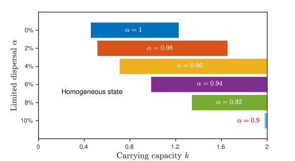
Figure 6: Inhomogeneous states of the metacommunity for different $\alpha$ values: Each horizontal bar denotes the parameter range of $k$ where the metacommunity exhibits inhomogeneous stable steady (asynchronous alternative) states. Other parameters are $\beta=1,r=0.5$, $a=1$, $c=0.5$, $b=0.16$, $m=0.2$, $d_{v}=0.001$ and $d_{h}=1$.

III.2 limiting predator dispersal along with local interaction

In this section, we investigate the influence of the limited predator dispersal and a local parameter (carrying capacity) on the dynamics of the metacommunity for $\beta=1$. The predator density is depicted in the bifurcation diagram as a function of the carrying capacity $k$ (see Fig. 5). The prey and predator dispersal rates are fixed as $d_{v}=0.001$ and $d_{h}=1$, respectively. The dynamical states are the same as in Fig. 2. The trivial steady state lose its stability via a transcritical bifurcation at $k=k_{TB}$ leading to a nontrivial homogeneous steady state, which undergoes a supercritical Hopf bifurcation (HB1) resulting in stable homogeneous oscillation and an unstable steady state at $k=0.4$ for $\alpha=1$ (see Fig. 5(a)). Using the standard linear stability analysis around the homogeneous steady state $\left(\frac{kr+kd_{v}(\beta-1)}{r},0,\frac{kr+kd_{v}(\beta-1)}{r},0\right)$, the transcritical bifurcation at $k=k_{TB}$ can be deduced as

$$k_{TB}=\frac{b(d_{h}+m-\alpha d_{h})}{ac+d_{h}(\alpha-1)-m}.$$

Similarly, one can obtain the Hopf bifurcation

$$k_{HB}=\frac{b\left[ac+m+(1-\alpha)d_{h}\right]}{ac+(\alpha-1)d_{h}-m},$$

by performing a linear stability analysis around the homogeneous steady state $(V^{*},H^{*},V^{*},H^{*})$, where $V^{*}=\frac{bm+bd_{h}(1-\alpha)}{ac-m-d_{h}(1-\alpha)}$, $H^{*}=\frac{bc\left[ack(r+d_{v}(\beta-1))-\left(br+kr+kd_{v}(\beta-1)\right)\left(m+d_{h}(1-\alpha)\right)\right]}{k(ac-m+d_{h}(\alpha-1))^{2}}$. Note that for $\beta=\alpha=1$, the Hopf and pitchfork bifurcation points/curves can be reduced to that in Ref. Arumugam et al. (2021).

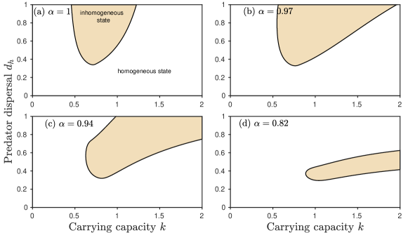
Figure 7: Two parameter bifurcation diagram in $(k,d_{h})$ parameter space for different $\alpha$ values: Here the shaded region indicates the parameter space where the metacommunity exhibits inhomogeneous stable states. Outside the shaded region, metacommunity exhibits only homogeneous state. For decreasing $\alpha$, inhomogeneous region is increased at first, and then decreased. Other parameters are $r=0.5$, $\alpha=1$, $\beta=0.5$, $B=0.16$, $m=0.2$ and $d_{v}=0.001$.

The stable homogeneous oscillatory state prevails in the entire explored range of $k\in[0.4,2]$. Subcritical Hopf bifurcation (HB2) emerges at $k=0.458$ resulting in unstable inhomogeneous oscillations and stable inhomogeneous steady states in the range of $k\in[0.458,1.043)$ leading to the existence of alternative stable states of the metacommunity. The latter lose its stability via a supercritical Hopf bifurcation (HB3) at $k=1.043$ resulting in stable inhomogeneous oscillations in the range $k\in[1.043,1.226)$ and unstable inhomogeneous steady states in the range $k\in[1.043,2.0]$, leaving behind the synchronized oscillatory states as the only stable state of the metacommunity A saddle-node bifurcation emerges at $k=1.226$. In the following, we will unravel the effect of limited dispersal as a function of the carrying capacity.

The bifurcation diagram elucidating the dynamical transitions of the metacommunity for $\alpha=0.95$ is depicted in Fig. 5(b). The dynamical states and their transitions are almost similar to that discussed in Fig. 5(a) for $\alpha=1.0$. Nevertheless, it is evident from the figure that the spread of the stable inhomogeneous steady (asynchronous alternative states) states increased to a larger extent, thereby increasing the degree of persistence of the metacommunity. However, this tendency, enhancing the spread of stable inhomogeneous steady states, of the degree of the dispersal persists up to a critical value and then the steady states lose its stability eventually resulting in the homogeneous (synchronous) oscillatory state as the only dynamical state as illustrated in Fig. 5(c) for $\alpha=0.9$. The spread of the stable inhomogeneous steady states for different values of $\alpha$ is depicted in Fig. 6 as a function of the carrying capacity $k$. It is also evident from the figure that the degree of the spread of inhomogeneous steady states increases initially for a small decrease in the dispersal and eventually decreases for further decrease in the dispersal beyond a critical value of $\alpha$.

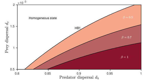
Figure 8: Two parameter bifurcation diagram in $d_{h}-d_{v}$ space at different $\beta$ values: Hopf bifurcation (HB1) curve separates the region into homogeneous and inhomogeneous stable states. Other parameter values are $r=0.5$, $k=0.5$, $a=1$, $c=0.5$, $b=0.16$, $m=0.2$ and $\alpha=0.985$.

The spread of the homogeneous and inhomogeneous states are shown in Fig. 7 as two parameter bifurcation diagrams in $(k,d_{h})$ parameter space for different degree of the predator dispersal. The homogeneous state prevails in the entire parameter space, where as the stable inhomogeneous steady states prevail only in the shaded regions leading to multistability. It is also evident from the figures that the spread of the stable inhomogeneous steady states increases for a small decrease in the degree of the predator dispersal up to a critical value of $\alpha$ and then it starts decreasing as a function of $\alpha$. The stable inhomogeneous steady states eventually destabilized from the entire parameter space, where it was stable, resulting in the homogeneous states as the only dynamical states of the metacommunity. Thus, the degree of limiting the predator dispersal results in increasing the persistence of the metacommuntiy until a critical value, above which it is endangered by the presence of homogeneous (synchronous) states as the only dynamical states of the metacommunity.

III.3 limiting prey dispersal

Now, we will investigate the effect of limiting the prey dispersal on the metacommunity dynamics as a function of the spatial parameter. For complete dispersal of the predators, that is for $\alpha=1$, the effect of limiting the prey dispersal on the metacommunity dynamics can be seen only in a narrow range of the parameter space. Hence, we have fixed $\alpha=0.985$, and depicted the two-parameter bifurcation diagram in the $(d_{h},d_{v})$ parameter space, where the effect of limiting the prey dispersal is well pronounced as evident from Fig. 8. Homogeneous oscillatory state is stable in the entire parameter space, while the inhomogeneous steady states are stable only in the shaded region. The transition from homogeneous oscillator state to inhomogeneous steady states is via the transcritical Hopf bifurcation (HB1) curve, which is obtained from XPPAUT. It is to be noted that for $\beta=1$, that is for uncontrolled prey dispersal, the spread of the inhomogeneous steady states is rather limited to smaller values of $d_{v}$. However, decreasing $\beta$, that is limiting the prey dispersal, manifests the stable inhomogeneous steady states in a larger region of the $(d_{h},d_{v})$ parameter space. For instance, the spread of the stable inhomogeneous steady states are depicted in Fig. 8 for $\beta=0.7$ and $0.5$. Thus, limiting the prey dispersal results in a large degree of the metacommunity persistence in contrast to the effect of limiting the predator dispersal. It is also to be noted that for different degrees of local parameter (carrying capacity), limiting the prey dispersal results in an increase in the metacommunity persistence.

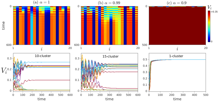
Figure 9: Spatio-temporal dynamics of a random (Erdos-Renyi) network consisting of 20 patches: Top panel shows the spatial dynamics of the metacommunity, whereas the bottom panel shows the respective time series. The metacommunity shows dynamical transitions from 10 clusters to 15 clusters, which further organized into a single cluster for decreasing degree of the limiting factor ($\alpha$). Here initial conditions are the same for each $\alpha$ value. Other parameters are fixed as $\beta=1$, $r=0.5$, $a=1$, $c=0.5$, $b=0.16$, $m=0.2$ and $d_{v}=0.001$.

III.4 limiting predator dispersal in a larger network

To elucidate the generic nature of our results, we consider an arbitrary network consisting of $N=20$ patches, whose governing equation is represented as

$$\frac{dV_{i}}{dt} =rV_{i}\left(1-\frac{V_{i}}{k}\right)-\frac{aV_{i}}{V_{i}+b}H_{i}+\frac{d_{v}}{d_{j}}\sum_{j=1}^{N}g_{ij}\left(\beta V_{j}-V_{i}\right)\;,$$ (5a)

$$\frac{dH_{i}}{dt} =\frac{caV_{i}}{V_{i}+b}H_{i}-mH_{i}+\frac{d_{h}}{d_{j}}\sum_{j=1}^{N}g_{ij}\left(\alpha H_{j}-H_{i}\right)\;,$$ (5b)

where $i=1,\ldots,N$. $g_{ij}$ encodes the topology of the underlying network. $g_{ij}=g_{ji}=1$, if $i$th and $j$th oscillators are connected, otherwise $g_{ij}=g_{ji}=0$. $d_{j}=\sum_{j=1}^{N}g_{ij}$ corresponds to the degree of the $j$th oscillator. The other parameters are the same as in Eq. (1). We have fixed the values of the parameters as $\beta=1.0,r=0.5$, $a=1$, $c=0.5$, $b=0.16$, $m=0.2,d_{h}=1$ $k=0.5$ and $d_{v}=0.001$. The dynamics of a random (Erdos-Renyi) network is depicted as spatiotemporal and time series plots in Fig. 9 for different degree of the predator dispersal. The network exhibits a ten cluster state, corresponding to ten stable steady states, for $\alpha=1$ as evident from the spatiotemporal and time series plots in Fig. 9(a). Nevertheless, decreasing the degree of dispersal to $\alpha=0.99$ results in increase in the number of clusters (see Fig. 9(b)). Note that the multi-cluster state corresponds to the alternative states of the metacommunity elucidating a high degree of their persistence. However, further decrease in the degree of the dispersal decreases the number of multi-cluster and eventually manifests as a single cluster state, as depicted in Fig. 9(c) for $\alpha=0.9$, at a critical value of $\alpha$ signaling a low degree of the metacommunity persistence.

The number of clusters is depicted as a function of the limiting factor $\alpha$ in Fig. 10(a) for the same values of the parameters as in Fig. 9. The size of the multi-cluster states initially varies for small decrease in the limiting factor and eventually decreases resulting in a single cluster state (homogeneous state) at a critical value of $\alpha=\alpha_{c}=0.907$. Thus, it is evident that the observed results of the two patch metacommunity hold for a random network of metacommunity thereby corroborating the generic nature of the results.

Denoting $\rho_{j}$’s ($j=1,2,\ldots,N$) as the eigenvalues of the connectivity matrix $g_{ij}$, characterizing an arbitrary network, which can be ordered as $1.0=\rho_{1}\geq\rho_{2}\geq\ldots\geq-1/(N-1)\geq\rho_{N}\geq-1.0$ Atay (2006). The smallest bounding eigenvalue of the connectivity matrix $g_{ij}$ corresponding to the random network employed in Figs. 9 and 10(a) is found to be $\rho_{N}=-0.987$. It is known that the role of coupling topology on the stability of the homogeneous steady state is determined by $\rho_{N}$ Zou et al. (2013, 2021), which completely characterizes the effect of the connection topology corresponding to an arbitrary network. We have depicted the critical value of the limiting factor $\alpha_{c}$ as a function of $\rho_{N}$ met in Fig. 10(b), which elucidates that our results are generic to any arbitrary network. Note that the entire range of $\rho_{N}\in[-1,0]$ captures all possible coupling topologies. It is to be noted that limiting the prey dispersal rate always results in multi-cluster states (inhomogeneous steady state) promoting metacommunity persistence and hence the above analysis of calculating $\alpha_{c}$ cannot be applied to this case.

Further, different networks can be constructed for the same probability of rewiring ‘$p$’ from complex networks perspective. Noted that the range of $p\in[0,1]$ covers the entire class of network topologies from regular, small world to random (scale-free) networks Watts and Strogatz (1998). The critical value of $\alpha$ is depicted in Fig. 11 as a function of $p$ with error bars characterizing the effect of various network sizes $N$. Specifically, we have chosen $N=20$ to $500$ in steps of $10$. The mean of all the critical values of the limiting factor corresponding to each $N$ is indicated by the filled circle for each $p$, while their variance is denoted by the error bars. Inset in Fig. 11 clearly depicts the error bars. The critical value of the limiting factor in the entire range of $p$ again corroborates the generic nature of our results.

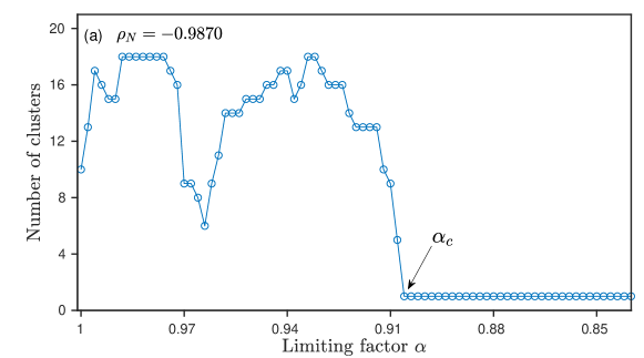
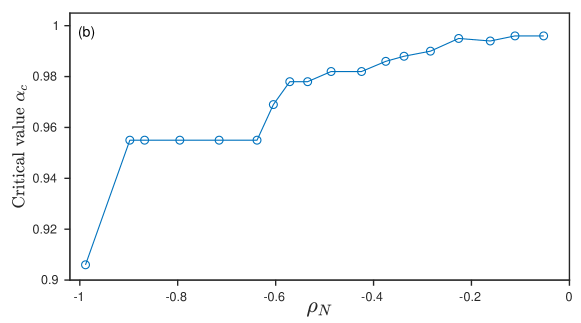
Figure 10: (a) Number of clusters as a function of the limiting factor $\alpha$ for a random network of $20$ nodes showing the transition from inhomogeneous steady states to homogeneous steady state, and (b) $\alpha_{c}$ as a function of the least bounding eigenvalue $\rho_{N}\in[-1,0]$ of the connectivity matrix $g_{ij}$, characterizing the entire class of complex networks

.

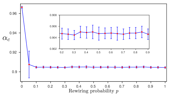
Figure 11: The critical value of predator limiting factor $\alpha_{c}$ as a function of the probability of rewiring $p\in[0,1]$ corresponding to the entire class of complex networks. Mean of all the critical values of the limiting factor corresponding to each $N$ is indicated by the filled circle for each $p$, while their variance is denoted by the error bars. Inset in the specific range of $p$ to clearly depict the error bars.

IV Discussion

In this study, we have addressed how limiting both predator and prey dispersal of a spatially distributed community affects its stability and persistence. Using the homogeneous (synchronized) and inhomogeneous (asynchronized) dynamical states of a diffusively coupled predator-prey metacommunity, we have elucidated the importance of controlled dispersal at local and spatial scales. At spatial scale, a small decrease in the predator immigration through the limiting factor reduces the metacommunity persistence by inducing the homogeneous state. On the other hand, at local scale, metacommunity persistence is increased for a small decrease in the predator immigration up to a critical value and then decreases for further increase in the degree of the limited predator dispersal. Moreover, our findings revealed that there exists a critical value for the limiting factor, below which metacommunity persists and above which metacommunity goes to a high risk state. However, limiting the prey dispersal promotes inhomogeneous steady states in a large region of the parameter space, thereby increasing the metacommunity persistence both at spatial and local scales. Further, we have showed the similar qualitative dynamics for an entire class of complex networks consisting of a large number of patches illustrating the robustness of our results, which remains unaltered in a large range of model parameters. Thus, our findings revealed that dispersal-dependent responses strongly influence the metacommunity persistence. Note that the spread of homogeneous and inhomogeneous steady states in the one-parameter bifurcation diagrams and two phase diagrams only get rescaled for the rescaled model (2).

Dispersal is a fundamental process for structuring natural ecosystems and it is widely recognized in conservation and ecosystem management Blasius et al. (1999); Holland and Hastings (2008). Since dispersal can rescue local populations from complete extinction, it is an important stabilizing mechanism for various ecological communities. However, dispersal induces synchrony among spatially connected populations which can elevate a high risk of extinction as compare to asynchronized dynamics Briggs and Hoopes (2004); Liebhold et al. (2004). Hence, theoretical understanding of population synchrony controlled by dispersal received a great attention. Numerous theoretical studies have addressed the factors and mechanisms of synchrony using various coupling strategies Kendall et al. (2000); Ripa (2000); Goldwyn and Hastings (2008); Arumugam et al. (2016). Our study revealed the synchronized and asynchronized dynamics of the metacommunity through a control on the diffusive dispersal. In particular, a decrease in the species immigration destabilizes the metacommunity through synchronized behaviour. Dispersal stabilizes the metacommunity through a source-sink behaviour whereby some patches have a high population abundance and others have a low population abundance Dias (1996). Various inhomogeneous dynamical states shown in this study represent the source-sink behaviour, which in turn influences the metacommunity persistence.

“Paradox of enrichment”, referring the existence of high-amplitude extinction-prone cycles due to increasing carrying capacity, can destabilize the ecological community (Rosenzweig, 1971). Our findings on varying carrying capacity with a controlled dispersal elucidated the solution to the “paradox of enrichment”. In particular, our results are in line with previous studies that dispersal can prevent the extinction prone cycles by creating inhomogeneous states and provide a solution to the paradox of enrichment (Jansen, 1995; Hauzy et al., 2013; Gounand et al., 2014). In addition, our findings revealed that the inhomogeneous states can be manifested as homogeneous state by limiting the dispersal. Thus, limiting the dispersal offer insights to understand the stability and persistence of a spatially distributed community through synchronized and asynchronized dynamics.

In summary, this study presents the effect of limiting dispersal on metacommunity persistence at local and spatial scales. The dynamics that we observe may apply to other ecological scenarios such as environmental stochasticity, spatial heterogeneity, and higher tropical interactions (i.e., foodweb). Since these ecological scenarios increase the complexity of system, a further investigation is required to understand how limiting the dispersal influences the stability of ecological communities. Overall, this study offers new insights on the stability and persistence of a spatially distributed ecological community.

V Acknowledgements

S. R. C. and R. A. acknowledges IISER-TVM for the financial support. W.Z. acknowledges support from Research Starting Grants from South China Normal University (Grant No. 8S0340), the Natural Science Foundation of Guangdong Province, China (Grant No. 2019A1515011868), and the National Natural Science Foundation of China (Grant No. 12075089). V. K. C. thank DST, New Delhi for computational facilities under the DST-FIST programme (SR/FST/PS-1/2020/135) to the Department of Physics. The work of V. K. C. is also supported by the SERB-DST-MATRICS Grant No. MTR/2018/000676 and CSIR Project under Grant No. 03(1444)/18/EMR-II. DVS is supported by the DST-SERB-CRG Project under Grant No. CRG/2021/000816.

References

- Pikovsky et al. (2001) A. Pikovsky, M. Rosenblum, and J. Kurths, Synchronization: A Universal Concept in Nonlinear Sciences, Cambridge nonlinear science series (Cambridge University Press, 2001).
- Izhikevich (2007) E. Izhikevich, Dynamical Systems in Neuroscience (MIT Press, 2007).
- Blasius et al. (1999) B. Blasius, A. Huppert, and L. Stone, Nature 399, 354 (1999).
- Liebhold et al. (2004) A. Liebhold, W. D. Koenig, and O. N. Bjørnstad, Annual Review of Ecology, Evolution, and Systematics 35, 467 (2004).
- Ranta et al. (1995) E. Ranta, V. Kaitala, J. Lindström, and H. Linden, Proceedings of the Royal Society of London. Series B: Biological Sciences 262, 113 (1995).
- Briggs and Hoopes (2004) C. J. Briggs and M. F. Hoopes, Theoretical population biology 65, 299 (2004).
- Goldwyn and Hastings (2008) E. Goldwyn and A. Hastings, Theoretical population biology 73, 395 (2008).
- Ranta et al. (1997) E. Ranta, V. Kaitala, J. Lindström, and E. Helle, Oikos , 136 (1997).
- Kendall et al. (2000) B. E. Kendall, O. N. Bjørnstad, J. Bascompte, T. H. Keitt, and W. F. Fagan, The American Naturalist 155, 628 (2000).
- Heino et al. (1997) M. Heino, V. Kaitala, E. Ranta, and J. Lindström, Proceedings of the Royal Society of London. Series B: Biological Sciences 264, 481 (1997).
- Holland and Hastings (2008) M. D. Holland and A. Hastings, Nature 456, 792 (2008).
- Doebeli (1995) M. Doebeli, Theoretical population biology 47, 82 (1995).
- Hanski (1998) I. Hanski, Nature 396, 41 (1998).
- Hanski (1999) I. Hanski, Metapopulation Ecology (Oxford University Press, New York, 1999).
- Wang and Loreau (2016) S. Wang and M. Loreau, Ecology Letters 19, 510 (2016).
- McPeek and Holt (1992) M. A. McPeek and R. D. Holt, The American Naturalist 140, 1010 (1992).
- Doebeli and Ruxton (1997) M. Doebeli and G. D. Ruxton, Evolution 51, 1730 (1997).
- Travis et al. (2013) J. M. Travis, M. Delgado, G. Bocedi, M. Baguette, K. Bartoń, D. Bonte, et al., Oikos 122, 1532 (2013).
- Fussmann et al. (2014) K. E. Fussmann, F. Schwarzmüller, U. Brose, A. Jousset, and B. C. Rall, Nature Climate Change 4, 206 (2014).
- Walther et al. (2002) G. Walther, E. Post, P. Convey, A. Menzel, C. Parmesan, T. J. C. Beebee, et al., Nature 416, 389 (2002).
- Parmesan (2006) C. Parmesan, Annual Review of Ecology, Evolution, and Systematics 37, 637 (2006).
- Berg et al. (2010) M. P. Berg, E. T. Kiers, G. Driessen, M. Van Der Heijden, B. W. Kooi, F. Kuenen, M. Liefting, H. A. Verhoef, and J. Ellers, Global Change Biology 16, 587 (2010).
- Walther (2010) G.-R. Walther, Philosophical Transactions of the Royal Society B: Biological Sciences 365, 2019 (2010).
- Reed et al. (2011) T. E. Reed, D. E. Schindler, and R. S. Waples, Conservation Biology 25, 56 (2011).
- Mueller et al. (2013) T. Mueller, R. B. O’Hara, S. J. Converse, R. P. Urbanek, and W. F. Fagan, Science 341, 999 (2013).
- Püttker et al. (2011) T. Püttker, A. A. Bueno, C. dos Santos de Barros, S. Sommer, and R. Pardini, PLoS One 6, e27963 (2011).
- Rosenzweig and MacArthur (1963) M. L. Rosenzweig and R. H. MacArthur, The American Naturalist 97, 209 (1963).
- Dutta and Banerjee (2015) P. S. Dutta and T. Banerjee, Phys. Rev. E 92, 042919 (2015).
- Arumugam et al. (2016) R. Arumugam, P. S. Dutta, and T. Banerjee, Phys. Rev. E 94, 022206 (2016).
- Arumugam and Dutta (2018) R. Arumugam and P. S. Dutta, Phys. Rev. E 97, 062217 (2018).
- Arumugam et al. (2021) R. Arumugam, V. K. Chandrasekar, and D. V. Senthilkumar, Phys. Rev. E 104, 024202 (2021).
- Ermentrout (2002) B. Ermentrout, Simulating, Analyzing, and Animating Dynamical Systems (Society for Industrial and Applied Mathematics, 2002).
- Atay (2006) F. M. Atay, Journal of Differential Equations 221, 190 (2006).
- Zou et al. (2013) W. Zou, D. V. Senthilkumar, M. Zhan, and J. Kurths, Phys. Rev. Lett. 111, 014101 (2013).
- Zou et al. (2021) W. Zou, D. V. Senthilkumar, M. Zhan, and J. Kurths, Physics Reports 931, 1 (2021).
- (36) Connectivity matrix characterized by can be obtained using Watts-Strogaz algorithm with a certain probability of rewiring of a regular network.
- Watts and Strogatz (1998) D. J. Watts and S. H. Strogatz, Nature 393, 440 (1998).
- Ripa (2000) J. Ripa, Oikos 89, 175 (2000).
- Dias (1996) P. C. Dias, Trends in Ecology & Evolution 11, 326 (1996).
- Rosenzweig (1971) M. L. Rosenzweig, Science 171, 385 (1971).
- Jansen (1995) V. A. A. Jansen, Oikos 74, 384 (1995).
- Hauzy et al. (2013) C. Hauzy, G. Nadin, E. Canard, I. Gounand, N. Mouquet, and B. Ebenman, PloS one 8, e82969 (2013).
- Gounand et al. (2014) I. Gounand, N. Mouquet, E. Canard, F. Guichard, C. Hauzy, and D. Gravel, The American Naturalist 184, 752 (2014).