Timelike minimal surfaces in the three-dimensional Heisenberg group

Abstract.

Timelike surfaces in the three-dimensional Heisenberg group with left invariant semi-Riemannian metric are studied. In particular, non-vertical timelike minimal surfaces are characterized by the non-conformal Lorentz harmonic maps into the de Sitter two sphere. On the basis of the characterization, the generalized Weierstrass type representation will be established through the loop group decompositions.

1. Introduction

Constant mean curvature surfaces in three-dimensional homogeneous spaces, specifically Thurston’s eight model spaces [27], have been intensively studied in recent years. One of the reasons is a seminal paper by Abresch-Rosenberg [1], where they introduced a quadratic differential, the so-called the Abresch-Rosenberg differential, analogous to the Hopf differential for surfaces in the space forms and showed that it was holomorphic for a constant mean curvature surface in various classes of three-dimensional homogeneous spaces, such as the Heisenberg group ${\rm Nil}_{3}$, the product spaces $\mathbb{S}^{2}\times\mathbb{R}$ and $\mathbb{H}^{2}\times\mathbb{R}$ etc, see [2] in detail. It is evident that holomorphic quadratic differentials are fundamental for study of global geometry of surfaces, [15]. On the one hand, Berdinsky-Taimanov developed integral representations of surfaces in three-dimensional homogeneous spaces by using the generating spinors and the nonlinear Dirac type equations, [3, 4]. They were natural generalizations of the classical Kenmotsu-Weierstrass representation for surfaces in the Euclidean three-space.

Combining the Abresch-Rosenberg differential and the nonlinear Dirac equation with generating spinors, in [12, 13], Dorfmeister, Inoguchi and the second named author of this paper have established the loop group method for minimal surfaces in ${\rm Nil}_{3}$, where the following left-invariant Riemannian metric has been considered on ${\rm Nil}_{3}$:

$$ds^{2}=dx_{1}^{2}+dx_{2}^{2}+\left(dx_{3}+\frac{1}{2}(x_{2}dx_{1}-x_{1}dx_{2})\right)^{2},$$

In particular, all non-vertical minimal surfaces in ${\rm Nil}_{3}$ have been constructed from holomorphic data, which have been called the holomorphic potentials, through the loop group decomposition, the so-called Iwasawa decomposition, and the construction has been commonly called the generalized Weierstrass type representation. In this loop group method, the Lie group structure of ${\rm Nil}_{3}$ and harmonicity of the left-translated normal Gauss map of a non-vertical surface, which obviously took values in a hemisphere in the Lie algebra of ${\rm Nil}_{3}$, were essential tools. To be more precise, a surface in ${\rm Nil}_{3}$ is minimal if and only if the left-translated normal Gauss map is a non-conformal harmonic map with respect to the hyperbolic metric on the hemisphere, that is, one considers the hemisphere as the hyperbolic two space not the two sphere with standard metric. Since the hyperbolic two space is one of the standard symmetric spaces and the loop group method of harmonic maps from a Riemann surface into a symmetric space have been developed very well [14], thus we have obtained the generalized Weierstrass type representation.

On the one had, it is easy to see that the three-dimensional Heisenberg group ${\rm Nil}_{3}$ can have the following left-invariant semi-Riemannian metrics:

$$ds^{2}_{\pm}=\pm dx_{1}^{2}+dx_{2}^{2}\mp\left(dx_{3}+\frac{1}{2}(x_{2}dx_{1}-x_{1}dx_{2})\right)^{2}.$$

Moreover in [25], it has been shown that the left-invariant semi-Riemannian metrics on ${\rm Nil}_{3}$ with $4$-dimensional isometry group only are the metrics $ds^{2}_{\mp}$. Therefore a natural problem is study of spacelike/timelike, minimal/maximal surfaces in ${\rm Nil}_{3}$ with the above semi-Riemannian metrics in terms of the generalized Weierstrass type representations.

In this paper we will consider timelike surfaces in ${\rm Nil}_{3}$ with the semi-Riemannian metric $ds^{2}_{-}$. For defining the Abresch-Rosenberg differential and the nonlinear Dirac equations with generating spinors, the para-complex structure on a timelike surface is essential, and we will systematically develop theory of timelike surfaces using the para-complex structure, the Abresch-Rosenberg differential and the nonlinear Dirac equations with generating spinors in Section 2. Then the first of the main results in this paper is Theorem 3.2, where non-vertical timelike minimal surfaces in ${\rm Nil}_{3}$ will be characterized in terms of harmonicity of the left-translated normal Gauss map. To be more precise, the left-translated normal Gauss map of a timelike surface takes values in the lower half part of the de Sitter two sphere $\widetilde{\mathbb{S}}^{2}_{1-}=\{(x_{1},x_{2},x_{3})\in\mathfrak{nil}_{3}=\mathbb{L}^{3}\mid-x_{1}^{2}+x_{2}^{2}+x_{3}^{2}=1,x_{3}<0\}$, but it is not a Lorentz harmonic map into $\widetilde{\mathbb{S}}^{2}_{1-}$ with respect to the standard metric on the de Sitter sphere. It will be shown that by combining two stereographic projections, the left-translated normal Gauss map can take values in the upper half part of the de Sitter two sphere with interchanging $x_{1}$ and $x_{2}$, that is, $\mathbb{S}^{2}_{1+}=\{(x_{1},x_{2},x_{3})\in\mathbb{L}^{3}\mid x_{1}^{2}-x_{2}^{2}+x_{3}^{2}=1,x_{3}>0\}$, see Figure 1, and it is a non-conformal Lorentz harmonic into $\mathbb{S}^{2}_{1+}$ if and only if the timelike surface is minimal, see Section 3.1 in details. Note that timelike minimal surfaces in $({\rm Nil}_{3},ds^{2}_{-})$ have been studied through the Weierstrass-Enneper type representation and the Björing problem in [17, 21, 7, 8, 26, 9, 10, 22, 19].

It has been known that timelike constant mean curvature surfaces in the three-dimensional Minkowski space $\mathbb{L}^{3}$ could be characterized by a Lorentz harmonic map into the de Sitter two space, [16, 18, 11, 5, 6]. In fact the Lorentz harmonicity of the unit normal of a timelike surface in $\mathbb{L}^{3}$ is equivalent to constancy of the mean curvature. Furthermore, the generalized Weierstrass type representation for timelike non-zero constant mean curvature surfaces has been established in [11]. In Theorem 4.1, we will show that two maps, which are given by the logarithmic derivative of one parameter family of moving frames of a non-conformal Lorentz harmonic map (the so-called extended frame) into $\mathbb{S}^{2}_{1+}$ with respect to an additional parameter (the so-called spectral parameter), define a timelike non-zero constant mean curvature surface in $\mathbb{L}^{3}$ and a non-vertical timelike minimal surface in ${\rm Nil}_{3}$, respectively.

From the view point of the loop group construction of Lorentz harmonic maps, the construction in [11] is sufficient, however, it is not enough for our study of timelike minimal surfaces in $({\rm Nil}_{3},ds_{-}^{2})$. As we have mentioned above, for defining the Abresch-Rosenberg differential and the nonlinear Dirac equation with generating spinors the para-complex structure is essential. Note that the para-complex structure has been used for study of timelike surface [28, 20]. We can then show that the Abresch-Rosenberg differential is para-holomorphic if a timelike surface has constant mean curvature, Theorem 2.6, which is analogous to the fundamental result of Abresch-Rosenberg.

As a by-product of utilizing the para-complex structure, it is easy to compare our construction with minimal surface in $({\rm Nil}_{3},ds^{2})$, where the complex structure has been used, and moreover, the generalized Weierstrass type representation can be understood in a unified way, that is, the Weierstrass data is just a $2$ by $2$ matrix-valued para-holomorphic function and a loop group decomposition of the solution of a para-holomorphic differential equation gives the extended frame of a non-conformal Lorentz harmonic map in $\mathbb{S}^{2}_{1+}$, Theorem 5.4. One of difficulties is that one needs to have appropriate loop group decompositions in the para-complex setting, that is, Birkhoff and Iwasawa decompositions. In Theorem 5.1, by identifying the double loop groups of $\mathrm{SL}_{2}\mathbb{R}$, that is $\Lambda{\rm SL}_{2}\mathbb{R}_{\sigma}\times\Lambda{\rm SL}_{2}\mathbb{R}_{\sigma}$ and the loop group of ${\rm SL}_{2}\mathbb{C}^{\prime}$, that is, $\Lambda^{\prime}{\rm SL}_{2}\mathbb{C}^{\prime}_{\sigma}$ (where $\mathbb{C}^{\prime}$ denotes the para-complex number) by a natural isomorphism, we will obtain such decompositions. Finally in Section 6, several examples will be shown by our loop group construction. In particular B-scroll type minimal surfaces in ${\rm Nil}_{3}$ will be established in Section 6.4. In Appendix A, we will discuss timelike constant mean curvature surfaces in $\mathbb{L}^{3}$, and in Appendix B, we will see the correspondence between our construction and the construction without the para-complex structure in [11].

2. Timelike surfaces in ${\rm Nil}_{3}$

In this section we will consider timelike surfaces in ${\rm Nil}_{3}$. In particular we will use the para-complex structure and the nonlinear Dirac equation for timelike surfaces. Finally the Lax pair type system for timelike surface will be shown.

2.1. ${\rm Nil}_{3}$ with indefinite metrics

The Heisenberg group is a $3$-dimensional Lie group

$${\rm Nil}_{3}(\tau)=(\mathbb{R}^{3}(x_{1},x_{2},x_{3}),\cdot)$$

for $\tau\neq 0$ with the multiplication

$$(x_{1},x_{2},x_{3})\cdot(y_{1},y_{2},y_{3})=(x_{1}+y_{1},x_{2}+y_{2},x_{3}+y_{3}+\tau(x_{1}y_{2}-y_{1}x_{2})).$$

The unit element of ${\rm Nil}_{3}(\tau)$ is $(0,0,0)$. The inverse element of $(x_{1},x_{2},x_{3})$ is $(-x_{1},-x_{2},-x_{3})$. The groups ${\rm Nil}_{3}(\tau)$ and ${\rm Nil}_{3}(\tau^{\prime})$ are isomorphic if $\tau\tau^{\prime}\neq 0$. The Lie algebra $\mathfrak{nil}_{3}$ of ${\rm Nil}_{3}(\tau)$ is $\mathbb{R}^{3}$ with the relations:

$$[e_{1},e_{2}]=2\tau e_{3},\quad[e_{2},e_{3}]=[e_{3},e_{1}]=0$$

with respect to the normal basis $e_{1}=(1,0,0),e_{2}=(0,1,0),e_{3}=(0,0,1)$. In this paper we consider the left invariant indefinite metric $ds_{-}^{2}$ for ${\rm Nil}_{3}$ as follows:

(2.1) $$ds_{-}^{2}=-(dx_{1})^{2}+(dx_{2})^{2}+\omega_{\tau}\otimes\omega_{\tau},$$

where $\omega_{\tau}=dx_{3}+\tau(x_{2}dx_{1}-x_{1}dx_{2})$. Moreover, we fix the real parameter $\tau$ as $\tau=1/2$ for simplicity. The vector fields $E_{k}\,(k=1,2,3)$ defined by

$$E_{1}=\partial_{x_{1}}-\frac{x_{2}}{2}\partial_{x_{3}},\quad E_{2}=\partial_{x_{2}}+\frac{x_{1}}{2}\partial_{x_{3}}\quad{\rm and}\quad E_{3}=\partial_{x_{3}}$$

are left invariant corresponding to $e_{1},e_{2},e_{3}$ and orthonormal to each other with the timelike vector $E_{1}$ with respect to the metric $ds_{-}^{2}$. The Levi-Civita connection $\nabla$ of $ds_{-}^{2}$ is given by

$$\begin{matrix}\vspace{2pt}\nabla_{E_{1}}E_{1}=0,&\nabla_{E_{1}}E_{2}=\frac{1}{2}E_{3},&\nabla_{E_{1}}E_{3}=-\frac{1}{2}E_{2},\\ \vspace{2pt}\nabla_{E_{2}}E_{1}=-\frac{1}{2}E_{3},&\nabla_{E_{2}}E_{2}=0,&\nabla_{E_{2}}E_{3}=-\frac{1}{2}E_{1},\\ \nabla_{E_{3}}E_{1}=-\frac{1}{2}E_{2},&\nabla_{E_{3}}E_{2}=-\frac{1}{2}E_{1},&\nabla_{E_{3}}E_{3}=0.\\ \end{matrix}$$

2.2. Para-complex structure

Let $\mathbb{C}^{\prime}$ be a real algebra spanned by $1$ and $i^{\prime}$ with following multiplication:

$$(i^{\prime})^{2}=1,\quad 1\cdot i^{\prime}=i^{\prime}\cdot 1=i^{\prime}.$$

An element of the algebra $\mathbb{C}^{\prime}=\mathbb{R}1\oplus\mathbb{R}i^{\prime}$ is called a para-complex number. For a para-complex number $z$ we can uniquely express $z=x+yi^{\prime}$ with some $x,y\in\mathbb{R}$. Similar to complex numbers, the real part $\operatorname{Re}z$, the imaginary part $\operatorname{Im}z$ and the conjugate $\bar{z}$ of $z$ are defined by

$$\operatorname{Re}z=x,\quad\operatorname{Im}z=y\quad{\rm and}\quad\bar{z}=x-yi^{\prime}.$$

For a para-complex number $z=x+yi^{\prime}\in\mathbb{C}^{\prime}$ there exists a para-complex number $w\in\mathbb{C}^{\prime}$ with $z^{1/2}=w$ if and only if

(2.2) $$x+y\geq 0\quad{\rm and}\quad x-y\geq 0.$$

In particular ${i^{\prime}}^{1/2}$ does not exist. Moreover, for a para-complex number $z=x+yi^{\prime}\in\mathbb{C}^{\prime}$, there exists a para-complex number $w\in\mathbb{C}^{\prime}$ such that $z=e^{w}$ if and only if

(2.3) $$x+y>0\quad{\rm and}\quad x-y>0.$$

Let $M$ be an orientable connected 2-manifold, $G$ a Lorentzian manifold and $f:M\to G$ a timelike immersion, that is, the induced metric on $M$ is Lorentzian. The induced Lorentzian metric defines a Lorentz conformal structure on $M$: for a timelike surface there exists a local para-complex coordinate system $z=x+yi^{\prime}$ such that the induced metric $I$ is given by $I=e^{u}dzd\bar{z}=e^{u}\left((dx)^{2}-(dy)^{2}\right)$. Then we can regard $M$ and $f$ as a Lorentz surface and a conformal immersion, respectively. The coordinate system $z$ is called the conformal coordinate system and the function $e^{u}$ the conformal factor of the metric with respect to $z$. For a para-complex coordinate system $z=x+yi^{\prime}$, the partial differentiations are defined by

$$\partial_{z}=\frac{1}{2}(\partial_{x}+i^{\prime}\partial_{y})\quad{\rm and}\quad\partial_{\bar{z}}=\frac{1}{2}(\partial_{x}-i^{\prime}\partial_{y}).$$

2.3. Structure equations

Let $f:M\to{\rm Nil}_{3}$ be a conformal immersion from a Lorentz surface $M$ into ${\rm Nil}_{3}$. Let us denote the inverse element of $f$ by $f^{-1}$. Then the $1$-form $\alpha=f^{-1}df$ satisfies the Maurer-Cartan equation:

(2.4) $$d\alpha+\frac{1}{2}[\alpha\wedge\alpha]=0.$$

For a conformal coordinate $z=x+yi^{\prime}$ defined on a simply connected domain $\mathbb{D}\subset M$, set $\Phi$ as

$$\Phi=f^{-1}f_{z}.$$

The function $\Phi$ takes values in the para-complexification $\mathfrak{nil}_{3}^{\mathbb{C}^{\prime}}$ of $\mathfrak{nil}_{3}$. Then $\alpha$ is expressed as

$$\alpha=\Phi dz+\overline{\Phi}d\bar{z}$$

and the Maurer-Cartan equation (2.4) as

(2.5) $$\Phi_{\bar{z}}-\overline{\Phi}_{z}+[\overline{\Phi},\Phi]=0.$$

Denote the para-complex extension of $ds_{-}^{2}=g=\sum_{i,j}g_{ij}dx_{i}dx_{j}$ to $\mathfrak{nil}_{3}^{\mathbb{C}^{\prime}}$ by the same letter. Then the conformality of $f$ is equivalent to

$$g(\Phi,\Phi)=0,\quad g(\Phi,\overline{\Phi})>0.$$

For the orthonormal basis $\{e_{1},e_{2},e_{3}\}$ of $\mathfrak{nil}_{3}$ we can expand $\Phi$ as $\Phi=\phi_{1}e_{1}+\phi_{2}e_{2}+\phi_{3}e_{3}$. Then the conformality of $f$ can be represented as

(2.6) $$-(\phi_{1})^{2}+(\phi_{2})^{2}+(\phi_{3})^{2}=0,\quad-\phi_{1}\overline{\phi_{1}}+\phi_{2}\overline{\phi_{2}}+\phi_{3}\overline{\phi_{3}}=\frac{1}{2}e^{u},$$

for some function $u$. The conformal factor is given by $e^{u}$. Conversely, for a $\mathfrak{nil}_{3}^{\mathbb{C}^{\prime}}$-valued function $\Phi=\sum_{k=1}^{3}\phi_{k}e_{k}$ on a simply connected domain $\mathbb{D}\subset M$ satisfying (2.5) and (2.6), there exists an unique conformal immersion $f:\mathbb{D}\to{\rm Nil}_{3}$ with the conformal factor $e^{u}$ satisfying $f^{-1}df=\Phi dz+\overline{\Phi}d\bar{z}$ for any initial condition in ${\rm Nil}_{3}$ given at some base point in $\mathbb{D}$.

Next we consider the equation for a timelike surface $f$ with constant mean curvature 0. For $f$ denote the unit normal vector field by $N$ and the mean curvature by $H$. The tension field $\tau(f)$ for $f$ is given by $\tau(f)$ = tr$(\nabla df)$ where $\nabla df$ is the second fundamental form for $(f,N)$. As well known the tension field of $f$ is related to the mean curvature and the unit normal by

(2.7) $$\tau(f)=2HN.$$

By left translating to $(0,0,0)$, we can see this equation rephrased as

(2.8) $$\Phi_{\bar{z}}+\overline{\Phi}_{z}+\left\{\Phi,\overline{\Phi}\right\}=e^{u}Hf^{-1}N$$

where $\{\cdot,\cdot\}$ is the bilinear symmetric map defined by

$$\left\{X,Y\right\}=\nabla_{X}Y+\nabla_{Y}X$$

for $X,Y\in\mathfrak{nil}_{3}$. In particular for a surface with the mean curvature 0, we have

(2.9) $$\Phi_{\bar{z}}+\overline{\Phi}_{z}+\left\{\Phi,\overline{\Phi}\right\}=0.$$

Conversely, for a $\mathfrak{nil}_{3}$-valued function $\Phi=\sum_{k=1}^{3}\phi_{k}e_{k}$ satisfying (2.5), (2.6) and (2.9) on a simply connected domain $\mathbb{D}$, there exists a conformal timelike surface $f:\mathbb{D}\to{\rm Nil}_{3}$ with the mean curvature $0$ and the conformal factor $e^{u}$ satisfying $f^{-1}df=\Phi dz+\overline{\Phi}d\bar{z}$ for any initial condition in ${\rm Nil}_{3}$ given at some base point in $\mathbb{D}$.

2.4. Nonlinear Dirac equation for timelike surfaces

Let us consider the conformality condition of an immersion $f$. We first prove the following lemma:

Lemma 2.1.

If a product $xy$ of two para-complex numbers $x,y\in\mathbb{C}^{\prime}$ has the square root, then there exists $\epsilon\in\{\pm 1,\pm i^{\prime}\}$ such that $\epsilon x$ and $\epsilon y$ have the square roots.

Proof.

By the assumption,

$$\operatorname{Re}(xy)\pm\operatorname{Im}(xy)\geq 0$$

holds, and a simple computation shows that it is equivalent to

$$(\operatorname{Re}(x)\pm\operatorname{Im}(x))(\operatorname{Re}(y)\pm\operatorname{Im}(y))\geq 0.$$

Then the claim follows. ∎

Since the first condition in (2.6) can be rephrased as

(2.10) $$\phi_{3}^{2}=(\phi_{1}+i\phi_{2})(\phi_{1}-i\phi_{2}),$$

and by Lemma 2.1, there exists $\epsilon\in\{\pm 1,\pm i^{\prime}\}$ such that $\epsilon(\phi_{1}+i\phi_{2})$ and $\epsilon(\phi_{1}-i\phi_{2})$ have the square roots. Therefore there exist para-complex functions $\overline{\psi_{2}}$ and $\psi_{1}$ such that

$$\phi_{1}+i\phi_{2}=2\epsilon\overline{\psi_{2}}^{2},\quad\phi_{1}-i\phi_{2}=2\epsilon{\psi_{1}}^{2}$$

hold. Then $\phi_{3}$ can be rephrased as $\phi_{3}=2\psi_{1}\overline{\psi_{2}}$. Let us compute the second condition in (2.6) by using $\{\psi_{1},\overline{\psi_{2}}\}$ as

$$-\phi_{1}\overline{\phi_{1}}+\phi_{2}\overline{\phi_{2}}+\phi_{3}\overline{\phi_{3}}=-2\epsilon\bar{\epsilon}(\psi_{1}\overline{\psi_{1}}-\epsilon\bar{\epsilon}\psi_{2}\overline{\psi_{2}})^{2}.$$

Since we have assumed that the left hand side is positive, $\epsilon$ takes values in

$$\epsilon\in\{\pm i^{\prime}\}.$$

Therefore without loss of generality, we have

(2.11) $$\phi_{1}=\epsilon\left((\overline{\psi_{2}})^{2}+(\psi_{1})^{2}\right),\>\phi_{2}=\epsilon i^{\prime}\left((\overline{\psi_{2}})^{2}-(\psi_{1})^{2}\right),\>\phi_{3}=2\psi_{1}\overline{\psi_{2}}.$$

Then the normal Gauss map $f^{-1}N$ can be represented in terms of the functions $\psi_{1}$ and $\psi_{2}$:

(2.12) $$f^{-1}N=2e^{-u/2}\left(-\epsilon\left(\psi_{1}\psi_{2}-\overline{\psi_{1}}\overline{\psi_{2}}\right)e_{1}+\epsilon i^{\prime}\left(\psi_{1}\psi_{2}+\overline{\psi_{1}}\overline{\psi_{2}}\right)e_{2}-\left(\psi_{2}\overline{\psi_{2}}-\psi_{1}\overline{\psi_{1}}\right)e_{3}\right),$$

where $e^{u/2}=2(\psi_{2}\overline{\psi_{2}}+\psi_{1}\overline{\psi_{1}})$. We can see that, using the functions $(\psi_{1},\psi_{2})$, the structure equations (2.5) and (2.8) are equivalent to the following nonlinear Dirac equation:

(2.13) $$\left(\begin{array}[]{ll}\partial_{z}\psi_{2}+\mathcal{U}\psi_{1}\\ -\partial_{\overline{z}}\psi_{1}+\mathcal{V}\psi_{2}\end{array}\right)=\left(\begin{array}[]{ll}0\\ 0\end{array}\right).$$

Here the Dirac potential $\mathcal{U}$ and $\mathcal{V}$ are given by

(2.14) $$\mathcal{U}=\mathcal{V}=-\frac{H}{2}e^{u/2}+\frac{i^{\prime}}{4}h$$

where

$$e^{u/2}=2\left(\psi_{2}\overline{\psi_{2}}+\psi_{1}\overline{\psi_{1}}\right)\quad{\rm and}\quad h=2\left(\psi_{2}\overline{\psi_{2}}-\psi_{1}\overline{\psi_{1}}\right).$$

Remark 2.2.

1. Without loss of generality, we can take $\psi_{2}\overline{\psi_{2}}+\psi_{1}\overline{\psi_{1}}$ as positive value, if necessary, by replacing $(\psi_{1},\psi_{2})$ into $(-i^{\prime}\psi_{1},i^{\prime}\psi_{2})$.

2. To prove the equations (2.5) and (2.8) from the nonlinear Dirac equation (2.13) with (2.14), the functions $e^{u/2}$ and $h$ in (2.14) and solutions $\psi_{k}\>(k=1,2)$ have to satisfy the relations

   $$e^{u/2}=2(\psi_{2}\overline{\psi_{2}}+\psi_{1}\overline{\psi_{1}}),\quad h=2(\psi_{2}\overline{\psi_{2}}-\psi_{1}\overline{\psi_{1}}).$$

For a timelike surface with the constant mean curvature $H=0$, the Dirac potential takes purely imaginary values. Then, by using (2.12), we have the following lemma.

Lemma 2.3.

Let $f:\mathbb{D}\to({\rm Nil}_{3},ds_{-}^{2})$ be a timelike surface with constant mean curvature $H=0$. Then the following statements are equivalent:

1. The Dirac potential $\mathcal{U}$ is not invertible at $p\in\mathbb{D}$.

2. The function $h$ is equal to zero at $p\in\mathbb{D}$.

3. $E_{3}$ is tangent to $f$ at $p\in\mathbb{D}$.

Remark 2.4.

The equivalence between $(2)$ and $(3)$ holds regardless of the value of $H$. In general, $\mathcal{U}$ is invertible if and only if $(\operatorname{Re}\mathcal{U})^{2}-(\operatorname{Im}\mathcal{U})^{2}\neq 0$.

Hereafter we will exclude the points where $\mathcal{U}$ is not invertible, that is, we will restrict ourselves to the case of

(2.15) $$\left({\rm Re}\,\mathcal{U}\right)^{2}-\left({\rm Im}\,\mathcal{U}\right)^{2}\neq 0.$$

Then, by using (2.3), the Dirac potentials can be written as

(2.16) $$\mathcal{U}=\mathcal{V}=\tilde{\epsilon}e^{w/2}$$

for some $\mathbb{C}^{\prime}$-valued function $w$ and $\tilde{\epsilon}\in\{\pm 1,\pm i^{\prime}\}$. In particular, if the mean curvature is zero and the function $h$ has positive values, then $\tilde{\epsilon}=i^{\prime}$.

2.5. Hopf differential and an associated quadratic differential

The Hopf differential $Adz^{2}$ is the $(2,0)$-part of the second fundamental form for $f$, that is,

$$A=g(\nabla_{\partial_{z}}f_{z},N).$$

A straightforward computation shows that the coefficient function $A$ is rephrased in terms of $\psi_{k}$ as follows:

$$A=2\{\psi_{1}(\overline{\psi_{2}})_{z}-\overline{\psi_{2}}(\psi_{1})_{z}\}-4i^{\prime}\psi_{1}^{2}(\overline{\psi_{2}})^{2}.$$

Next we define a para-complex valued function $B$ by

(2.17) $$B=\frac{1}{4}(2H-i^{\prime})\tilde{A},\quad\mbox{where}\quad\tilde{A}=A-\frac{\phi_{3}^{2}}{2H-i^{\prime}}.$$

Here $A$ and $\phi_{3}$ are the Hopf differential and the $e_{3}$-component of $f^{-1}f_{z}$ for $f$. It is easy to check the quadratic differential $Bdz^{2}$ is defined entirely and it will be called the Abresch-Rosenberg differential.

2.6. Lax pair for timelike surfaces

The nonlinear Dirac equation can be represented in terms of the Lax pair type system.

Theorem 2.5.

Let $\mathbb{D}$ be a simply connected domain in $\mathbb{C}^{\prime}$ and $f:\mathbb{D}\to{\rm Nil}_{3}$ a conformal timelike immersion for which the Dirac potential $\mathcal{U}$ satisfies (2.15). Then the vector $\widetilde{\psi}=(\psi_{1},\psi_{2})$ satisfies the system of equations

(2.18) $$\widetilde{\psi}_{z}=\widetilde{\psi}\widetilde{U},\quad\widetilde{\psi}_{\bar{z}}=\widetilde{\psi}\widetilde{V},$$

where

(2.19) $$\widetilde{U} =\begin{pmatrix}\frac{1}{2}w_{z}+\frac{1}{2}H_{z}\tilde{\epsilon}e^{-w/2}e^{u/2}&-\tilde{\epsilon}e^{w/2}\\ B\tilde{\epsilon}e^{-w/2}&0\end{pmatrix},$$

(2.20) $$\widetilde{V} =\begin{pmatrix}0&-\overline{B}\tilde{\epsilon}e^{-w/2}\\ \tilde{\epsilon}e^{w/2}&\frac{1}{2}w_{\bar{z}}+\frac{1}{2}H_{\bar{z}}\tilde{\epsilon}e^{-w/2}e^{u/2}\end{pmatrix}.$$

Here, $\tilde{\epsilon}\in\{\pm 1,\pm i^{\prime}\}$ is the number decided by (2.16). Conversely, every solution $\widetilde{\psi}$ to (2.18) with (2.16) and (2.14) is a solution of the nonlinear Dirac equation (2.13) with (2.14).

Proof.

By computing the derivative of the Dirac potential $\tilde{\epsilon}e^{w/2}$ with respect to $z$, we have

$$\frac{1}{2}w_{z}\tilde{\epsilon}e^{w/2}=-\frac{1}{2}H_{z}e^{u/2}+2i^{\prime}H\psi_{1}\psi_{2}(\overline{\psi}_{2})^{2}-\frac{2H-i^{\prime}}{2}\psi_{2}(\overline{\psi}_{2})_{z}-\frac{2H+i^{\prime}}{2}\overline{\psi_{1}}(\psi_{1})_{z}.$$

Multiplying the equation above by $\psi_{1}$ and using the function $B$ defined in (2.17), we derive

$$(\psi_{1})_{z}=\left(\frac{1}{2}w_{z}+\frac{1}{2}H_{z}\tilde{\epsilon}e^{-w/2}e^{u/2}\right)\psi_{1}+B\tilde{\epsilon}e^{-w/2}\psi_{2}.$$

The derivative of $\psi_{2}$ with respect to $z$ is given by the nonlinear Dirac equation. Thus we obtain the first equation of (2.18). We can derive the second equation of (2.18) in a similar way by differentiating the potential with respect to $\bar{z}$.

Conversely, if the vector $\widetilde{\psi}=(\psi_{1},\psi_{2})$ is a solution of (2.18), the terms of $(\psi_{1})_{\bar{z}}$ and $(\psi_{2})_{z}$ of (2.18) are the equations just we want. ∎

The compatibility condition of the above system is

(2.21) $$\frac{1}{2}w_{z\bar{z}}+e^{w}-B\overline{B}e^{-w}+\frac{1}{2}(H_{z\bar{z}}+p)\tilde{\epsilon}e^{-w/2}e^{u/2}=0,$$

(2.22) $$\overline{B}_{z}\tilde{\epsilon}e^{-w/2}=-\frac{1}{2}\overline{B}H_{z}e^{-w}e^{u/2}-\frac{1}{2}H_{\bar{z}}e^{u/2},$$

(2.23) $$B_{\bar{z}}\tilde{\epsilon}e^{-w/2}=-\frac{1}{2}BH_{\bar{z}}e^{-w}e^{u/2}-\frac{1}{2}H_{z}e^{u/2},$$

where $p=H_{z}(-w/2+u/2)_{\bar{z}}$ for the (1,1)-entry and $p=H_{\bar{z}}(-w/2+u/2)_{z}$ for the (2,2)-entry. From the above compatibility conditions we have the following:

Theorem 2.6.

For a constant mean curvature timelike surface in ${\rm Nil}_{3}$ which has the Dirac potential invertible anywhere, the Abresch-Rosenberg differential is para-holomorphic.

Remark 2.7.

To obtain a timelike immersion for solutions $w,B$ and $H$ of the compatibility condition (2.21), (2.22) and (2.23), a solution $\widetilde{\psi}=(\psi_{1},\psi_{2})$ of (2.18) has to satisfy

$$\tilde{\epsilon}e^{w/2}=-H(\psi_{2}\overline{\psi_{2}}+\psi_{1}\overline{\psi_{1}})+\frac{i^{\prime}}{2}(\psi_{2}\overline{\psi_{2}}-\psi_{1}\overline{\psi_{1}}).$$

This gives an overdetermined system and it seems not easy to find a general solution for arbitrary $H$, but for minimal surfaces we will show that it will be automatically satisfied.

3. Timelike minimal surfaces in ${\rm Nil}_{3}$

A timelike surface in ${\rm Nil}_{3}$ with the constant mean curvature $H=0$ is called a timelike minimal surface. By Theorem 2.6, the Abresch-Rosenberg differential for a timelike minimal surface is para-holomorphic. For example the triple $B=0,H=0$ and $e^{w}=16/(1+16z\bar{z})^{2}$ is a solution of the compatibility condition (2.21), (2.22) and (2.23). In fact these are derived from a horizontal plane

(3.1) $$f(z)=\left(\frac{2i^{\prime}(z-\bar{z})}{1+z\bar{z}},\frac{2(z+\bar{z})}{1+z\bar{z}},0\right).$$

Thus the horizontal plane (3.1) is a timelike minimal surface in ${\rm Nil}_{3}$. We will give examples of timelike minimal surfaces in Section 6. In this section we characterize timelike minimal surfaces in terms of the normal Gauss map.

3.1. The normal Gauss map

For a timelike surface in ${\rm Nil}_{3}$, the normal Gauss map is given by (2.12). Clearly it takes values in de Sitter two sphere $\widetilde{\mathbb{S}}^{2}_{1}\subset\mathfrak{nil}_{3}$:

$$\widetilde{\mathbb{S}}^{2}_{1}=\left\{x_{1}e_{1}+x_{2}e_{2}+x_{3}e_{3}\in\mathfrak{nil}_{3}\mid-x_{1}^{2}+x_{2}^{2}+x_{3}^{2}=1\right\}.$$

From now on we will assume that the function $h$ takes positive values, that is, the image of the normal Gauss map is in lower half part of the de Sitter two sphere. Moreover, we assume that the timelike surface has the pair of functions $(\psi_{1},\psi_{2})$ of the formula (2.11) with $\epsilon=i^{\prime}$. If the function $h$ takes negative values, or if the functions $(\psi_{1},\psi_{2})$ are given with $\epsilon=-i^{\prime}$, by a similar to the case of $h>0$ and $\epsilon=i^{\prime}$, we can get same results.

The normal Gauss map $f^{-1}N$ can be considered as a map into another de Sitter two sphere in the Minkowski space

$$\mathbb{S}^{2}_{1}=\left\{(x_{1},x_{2},x_{3})\in\mathbb{L}^{3}\mid x_{1}^{2}-x_{2}^{2}+x_{3}^{2}=1\right\}\subset\mathbb{L}^{3}_{(+,-,+)}$$

through the stereographic projections from $(0,0,1)\in\widetilde{\mathbb{S}}^{2}_{1}\subset\mathfrak{nil}_{3}$:

$$\pi_{\mathfrak{nil}}^{+}:\mathfrak{nil}_{3}\supset\widetilde{\mathbb{S}}^{2}_{1}\ni x_{1}e_{1}+x_{2}e_{2}+x_{3}e_{3}\mapsto\left(\frac{x_{1}}{1-x_{3}},\frac{x_{2}}{1-x_{3}},0\right)=\frac{x_{1}}{1-x_{3}}+i^{\prime}\frac{x_{2}}{1-x_{3}}\in\mathbb{C}^{\prime}$$

and from $(0,0,-1)\in\mathbb{S}^{2}_{1}\subset\mathbb{L}^{3}_{(+,-,+)}$:

$$\pi_{\mathbb{L}^{3}}^{-}:\mathbb{L}^{3}_{(+,-,+)}\supset\mathbb{S}^{2}_{1}\ni(x_{1},x_{2},x_{3})\mapsto\left(\frac{x_{1}}{1+x_{3}},\frac{x_{2}}{1+x_{3}},0\right)=\frac{x_{1}}{1+x_{3}}+i^{\prime}\frac{x_{2}}{1+x_{3}}\in\mathbb{C}^{\prime}.$$

In particular, the inverse map $(\pi_{\mathbb{L}^{3}}^{-})^{-1}$ is given by

$$(\pi_{\mathbb{L}^{3}}^{-})^{-1}(g)=\left(\frac{2\operatorname{Re}g}{1+g\overline{g}},\frac{2\operatorname{Im}g}{1+g\overline{g}},\frac{1-g\overline{g}}{1+g\overline{g}}\right)$$

for $g=\left(\operatorname{Re}g,\operatorname{Im}g,0\right)\in\mathbb{C}^{\prime}$. Since the normal Gauss map takes values in the lower half of the de Sitter two sphere in $\mathfrak{nil}_{3}$, the image under the projection $\pi_{\mathfrak{nil}}^{+}$ is in the region enclosed by four hyperbolas, see Figure 1. Two of the four hyperbolas correspond to the vertical points, that is, the points where $h$ vanishes, and the others correspond to the infinite-points, that is, the points where the first fundamental form degenerates. Since first and second sign of metrics of ${\rm Nil}_{3}$ and $\mathbb{L}^{3}_{(+,-,+)}$ are interchanged, the image of each hyperbola under the inverse map $(\pi^{-}_{\mathbb{L}^{3}})^{-1}$ plays the other role.

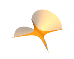
Figure 1. The upper half part of the de Sitter two sphere $\mathbb{S}^{2}_{1}$ (left) and its stereographic projection (middle), and the stereographic projection of the lower half part of $\tilde{\mathbb{S}^{2}_{1}}$ (right).

Define a map $g$ by the composition of the stereographic projection $\pi_{\mathfrak{nil}}^{+}$ with $f^{-1}N$, and then we obtain

$$g=i^{\prime}\frac{\overline{\psi_{1}}}{\psi_{2}}\in\mathbb{C}^{\prime}.$$

Thus the normal Gauss map can be represented as

$$f^{-1}N=\frac{1}{1-g\overline{g}}\left(2\operatorname{Re}(g)e_{1}+2\operatorname{Im}(g)e_{2}-(1+g\overline{g})e_{3}\right)$$

and

(3.2) $$(\pi_{\mathbb{L}^{3}}^{-})^{-1}\circ\pi_{\mathfrak{nil}}^{+}\circ f^{-1}N=\frac{1}{\psi_{2}\overline{\psi_{2}}-\psi_{1}\overline{\psi_{1}}}\left(-2\operatorname{Im}(\psi_{1}\psi_{2}),2\operatorname{Re}(\psi_{1}\psi_{2}),\psi_{2}\overline{\psi_{2}}+\psi_{1}\overline{\psi_{1}}\right).$$

Let $\mathfrak{su}_{1,1}^{\prime}$ be the special para-unitary Lie algebra defined by

$$\mathfrak{su}_{1,1}^{\prime}=\left\{\begin{pmatrix}ai^{\prime}&\bar{b}\\ b&-ai^{\prime}\end{pmatrix}\mid a\in\mathbb{R},b\in\mathbb{C}^{\prime}\right\}$$

with the usual commutator of the matrices. We assign the following indefinite product on $\mathfrak{su}_{1,1}^{\prime}$:

$$\langle X,Y\rangle:=2{\rm tr}(XY).$$

Then we can identify the Lie algebra $\mathfrak{su}_{1,1}^{\prime}$ with $\mathbb{L}^{3}_{(+,-,+)}$ isometrically by

(3.3) $$\mathfrak{su}_{1,1}^{\prime}\ni\frac{1}{2}\begin{pmatrix}ri^{\prime}&-p-qi^{\prime}\\ -p+qi^{\prime}&-ri^{\prime}\end{pmatrix}\longleftrightarrow(p,q,r)\in\mathbb{L}^{3}_{(+,-,+)}.$$

Let ${\rm SU}_{1,1}^{\prime}$ be the special para-unitary group of degree two corresponding to $\mathfrak{su}_{1,1}^{\prime}$:

$${\rm SU}_{1,1}^{\prime}=\left\{\begin{pmatrix}\alpha&\beta\\ \bar{\beta}&\bar{\alpha}\end{pmatrix}\mid\alpha,\beta\in\mathbb{C}^{\prime},\alpha\bar{\alpha}-\beta\bar{\beta}=1\right\}.$$

By the identification (3.3), the represented normal Gauss map (3.2) is equal to

$$(\pi_{\mathbb{L}^{3}}^{-})^{-1}\circ\pi_{\mathfrak{nil}}^{+}\circ f^{-1}N=\frac{i^{\prime}}{2}\operatorname{Ad}(F)\begin{pmatrix}1&0\\ 0&-1\end{pmatrix},$$

where $F$ is a ${\rm SU}_{1,1}^{\prime}$-valued map defined by

(3.4) $$F=\frac{1}{\sqrt{\psi_{2}\overline{\psi_{2}}-\psi_{1}\overline{\psi_{1}}}}\begin{pmatrix}\overline{\psi_{2}}&\overline{\psi_{1}}\\ \psi_{1}&\psi_{2}\end{pmatrix}.$$

The ${\rm SU}_{1,1}^{\prime}$-valued function $F$ defined as above is called a frame of the normal Gauss map $f^{-1}N$.

Remark 3.1.

In general a frame of the normal Gauss map $f^{-1}N$ is not unique, that is, for some frame $F$, there is a freedom of ${\rm SU}_{1,1}^{\prime}$-valued initial condition $F_{0}$ and ${\rm U}_{1}^{\prime}$-valued map $k$ such that $F_{0}Fk$ is an another frame. In this paper we use the particular frame in (3.4), since arbitrary choice of initial condition does not correspond to a given timelike surface $f$.

3.2. Characterization of timelike minimal surfaces

Let $F$ be the frame defined in (3.4) of the normal Gauss map $f^{-1}N$. By taking the gauge transformation

$$F\mapsto F\begin{pmatrix}e^{-w/4}&0\\ 0&e^{-w/4}\end{pmatrix},$$

we can see the system (2.18) is equivalent to the matrix differential equations

(3.5) $$F_{z}=FU,\quad F_{\bar{z}}=FV,$$

where

$$U =\begin{pmatrix}\frac{1}{4}w_{z}+\frac{1}{2}H_{z}\tilde{\epsilon}e^{-w/2}e^{u/2}&-\tilde{\epsilon}e^{w/2}\\ B\tilde{\epsilon}e^{-w/2}&-\frac{1}{4}w_{z}\end{pmatrix},$$

$$V =\begin{pmatrix}-\frac{1}{4}w_{\bar{z}}&-\bar{B}\tilde{\epsilon}e^{-w/2}\\ \tilde{\epsilon}e^{w/2}&\frac{1}{4}w_{\bar{z}}+\frac{1}{2}H_{\bar{z}}\tilde{\epsilon}e^{-w/2}e^{u/2}\end{pmatrix}.$$

We define a family of Maurer-Cartan forms $\alpha^{\mu}$ parameterized by $\mu\in\left\{e^{i^{\prime}t}\,|\,t\in\mathbb{R}\right\}$ as follows:

(3.6) $$\alpha^{\mu}:=U^{\mu}dz+V^{\mu}d\bar{z},$$

where

(3.7) $$U^{\mu} =\begin{pmatrix}\frac{1}{4}w_{z}+\frac{1}{2}H_{z}\tilde{\epsilon}e^{-w/2}e^{u/2}&-\mu^{-1}\tilde{\epsilon}e^{w/2}\\ \mu^{-1}B\tilde{\epsilon}e^{-w/2}&-\frac{1}{4}w_{z}\end{pmatrix},$$

(3.8) $$V^{\mu} =\begin{pmatrix}-\frac{1}{4}w_{\bar{z}}&-\mu\bar{B}\tilde{\epsilon}e^{-w/2}\\ \mu\tilde{\epsilon}e^{w/2}&\frac{1}{4}w_{\bar{z}}+\frac{1}{2}H_{\bar{z}}\tilde{\epsilon}e^{-w/2}e^{u/2}\end{pmatrix}.$$

Theorem 3.2.

Let $f$ be a conformal timelike immersion from a simply connected domain $\mathbb{D}\subset\mathbb{C}^{\prime}$ into ${\rm Nil}_{3}$ satisfying (2.15). Then the following conditions are mutually equivalent$:$

1. $f$ is a timelike minimal surface.

2. The Dirac potential $\mathcal{U}=\tilde{\epsilon}e^{w/2}=-\frac{H}{2}e^{u/2}+\frac{i^{\prime}}{4}h$ takes purely imaginary values.

3. $d+\alpha^{\mu}$ defines a family of flat connections on $\mathbb{D}\times{\rm SU}_{1,1}^{\prime}$.

4. The normal Gauss map $f^{-1}N$ is a Lorentz harmonic map into de Sitter two sphere $\mathbb{S}^{2}_{1}\subset\mathbb{L}^{3}_{(+,-,+)}$.

Proof.

The statement (3) holds if and only if

(3.9) $$(U^{\mu})_{\bar{z}}-(V^{\mu})_{z}+[V^{\mu},U^{\mu}]=0$$

for all $\mu\in\left\{e^{i^{\prime}t}\,|\,t\in\mathbb{R}\right\}$. The coefficients of ${\mu}^{-1},{\mu}^{0}$ and $\mu$ of (3.9) are as follows:

(3.10) $$\mbox{$\mu^{-1}$-part:}\;\;\frac{1}{2}H_{\bar{z}}e^{u/2}=0,\;\;B_{\bar{z}}+\frac{1}{2}BH_{\bar{z}}\tilde{\epsilon}e^{-w/2}e^{u/2}=0,$$

(3.11) $$\mbox{$\mu^{0}$-part:}\;\;\frac{1}{2}w_{z\bar{z}}+e^{w}-B\overline{B}e^{-w}+\frac{1}{2}(H_{z\bar{z}}+p)\tilde{\epsilon}e^{-w/2}e^{u/2}=0,$$

(3.12) $$\mbox{$\mu$-part:}\;\;\overline{B}_{z}+\frac{1}{2}\overline{B}H_{z}\tilde{\epsilon}e^{-w/2}e^{u/2}=0,\;\;\frac{1}{2}H_{z}e^{u/2}=0,$$

where $p$ is $H_{z}(-w/2+u/2)_{\bar{z}}$ for the $(1,1)$-entry and $H_{\bar{z}}(-w/2+u/2)_{z}$ for the $(2,2)$-entry, respectively. Since the equation in (3.11) is a structure equation for the immersion $f$, these are always satisfied, which in fact is equivalent to (2.21).

The equivalence of (1) and (2) is obvious.
We consider $(1)\Rightarrow(3)$. Since $f$ is timelike minimal, by Theorem 2.6, the Abresch-Rosenberg differential $Bdz^{2}$ is para-holomorphic. Hence, the equations (3.10), (3.11) and (3.12) hold. Consequently, the statement $(3)$ holds.

Next we show $(3)\Rightarrow(1)$. Assume that $d+\alpha^{\lambda}$ is flat, that is, (3.10), (3.11) and (3.12) are satisfied. Then it is easy to see that $H$ is constant. Furthermore, since $\alpha^{\mu}$ is valued in $\mathfrak{su}_{1,1}^{\prime}$, we can derive that the mean curvature $H$ is 0 by comparing (2,1)-entry with (1,2)-entry of $\alpha^{\mu}$.
Finally we consider the equivalence between (3) and (4). The condition (3) is (3.9) and it can be rephrased as

(3.13) $$d(*\alpha_{1})+[\alpha_{0}\wedge*\alpha_{1}]=0,$$

where $\alpha_{0}=\alpha^{\prime}_{\mathfrak{k}}dz+\alpha^{\prime\prime}_{\mathfrak{k}}d\bar{z}$ and $\alpha_{1}=\alpha^{\prime}_{\mathfrak{m}}dz+\alpha^{\prime\prime}_{\mathfrak{m}}d\bar{z}$ and $\mathfrak{su}_{1,1}^{\prime}$ has been decomposed as $\mathfrak{su}_{1,1}^{\prime}=\mathfrak{k}+\mathfrak{m}$ with

$$\mathfrak{k}=\left\{\begin{pmatrix}i^{\prime}r&0\\ 0&-i^{\prime}r\end{pmatrix}\mid r\in\mathbb{R}\right\},\quad\mathfrak{m}=\left\{\begin{pmatrix}0&-p-qi^{\prime}\\ -p+qi^{\prime}&0\end{pmatrix}\mid p,q\in\mathbb{R}\right\}.$$

Moreover $*$ denotes the Hodge star operator defined by

$$*dz=i^{\prime}dz,\quad*d\bar{z}=-i^{\prime}d\bar{z}.$$

It is known that by [23, Section 2.1], the harmonicity condition (3.13) is equivalent to the Lorentz harmonicity of the normal Gauss map $f^{-1}N=\tfrac{i^{\prime}}{2}F\sigma_{3}F^{-1}$ into the symmetric space $\mathbb{S}^{2}_{1}$. Thus the equivalence between (3) and (4) follows. ∎

From Theorem 3.2, we define the followings$:$

Definition 3.3.

1. For a timelike minimal surface $f$ in ${\rm Nil}_{3}$ with the frame $F$ in (3.4) of the normal Gauss map, let $F^{\mu}$ be a ${\rm SU}_{1,1}^{\prime}$-valued solution of the matrix differential equation $(F^{\mu})^{-1}dF^{\mu}=\alpha^{\mu}$ with $F^{\mu}|_{\mu=1}=F$. Then $F^{\mu}$ is called an extended frame of the timelike minimal surface $f$.

2. Let $\tilde{F}^{\mu}$ be a ${\rm SU}_{1,1}^{\prime}$-valued solution of $(\tilde{F}^{\mu})^{-1}d\tilde{F}^{\mu}=\alpha^{\mu}$. Then $\tilde{F}^{\mu}$ is called a general extended frame.

Note that an extended frame $F^{\mu}$ and a general extended frame $\tilde{F}^{\mu}$ are differ by an initial condition $F_{0}$, $\tilde{F}^{\mu}=F_{0}F^{\mu}$, and $F^{\mu}$ can be explicitly written as

(3.14) $$F^{\mu}=\frac{1}{\sqrt{\psi_{2}(\mu)\overline{\psi_{2}(\mu)}-\psi_{1}(\mu)\overline{\psi_{1}(\mu)}}}\begin{pmatrix}\overline{\psi_{2}(\mu)}&\overline{\psi_{1}(\mu)}\\ \psi_{1}(\mu)&\psi_{2}(\mu)\end{pmatrix},\quad$$

where $\psi_{j}(\mu=1)=\psi_{j}\;(j=1,2)$ are the original generating spinors of a timelike minimal surface $f$. For a timelike minimal surface, the Maurer-Cartan form $\alpha^{\mu}=U^{\mu}dz+V^{\mu}d\bar{z}$ of a general extended frame $\tilde{F}^{\mu}$ can be written explicitly as follows:

(3.15) $$U^{\mu}=\begin{pmatrix}\frac{1}{2}(\log h)_{z}&-\frac{i^{\prime}}{4}h\mu^{-1}\\ 4{i^{\prime}}Bh^{-1}\mu^{-1}&-\frac{1}{2}(\log h)_{z}\end{pmatrix},\quad V^{\mu}=\begin{pmatrix}-\frac{1}{2}(\log h)_{\bar{z}}&-4{i^{\prime}}\bar{B}h^{-1}\mu\\ \frac{i^{\prime}}{4}h\mu&\frac{1}{2}(\log h)_{\bar{z}}\end{pmatrix}.$$

4. Sym formula and duality between timelike minimal surfaces in three-dimensional Heisenberg group and timelike CMC surfaces in Minkowski space

In this section we will derive an immersion formula for timelike minimal surfaces in ${\rm Nil}_{3}$ in terms of the extended frame, the so-called Sym formula. Unlike the integral represetnation formula, the so-called Weierstrass type representation [21, 26, 10, 19], the Sym-formula will be given by the derivative of the extended frame with respect to the spectral parameter.

We define a map $\Xi:\mathfrak{su}_{1,1}^{\prime}\to\mathfrak{nil}_{3}$ by

(4.1) $$\Xi\left(x_{1}\mathcal{E}_{1}+x_{2}\mathcal{E}_{2}+x_{3}\mathcal{E}_{3}\right):=x_{1}e_{1}+x_{2}e_{2}+x_{3}e_{3}$$

where

(4.2) $$\mathcal{E}_{1}=\frac{1}{2}\begin{pmatrix}0&-i^{\prime}\\ i^{\prime}&0\end{pmatrix},\quad\mathcal{E}_{2}=\frac{1}{2}\begin{pmatrix}0&-1\\ -1&0\end{pmatrix},\quad\mathcal{E}_{3}=\frac{1}{2}\begin{pmatrix}i^{\prime}&0\\ 0&-i^{\prime}\end{pmatrix}.$$

Clearly, $\Xi$ is a linear isomorphism but not a Lie algebra isomorphism. Moreover, define a map $\Xi_{\mathfrak{nil}}:\mathfrak{su}_{1,1}^{\prime}\to{\rm Nil}_{3}$ as $\Xi_{\mathfrak{nil}}=\exp\circ\Xi$, explicitly

(4.3) $$\Xi_{\mathfrak{nil}}\left(\frac{1}{2}\begin{pmatrix}x_{3}i^{\prime}&-x_{2}-x_{1}i^{\prime}\\ -x_{2}+x_{1}i^{\prime}&-x_{3}i^{\prime}\end{pmatrix}\right)=(x_{1},x_{2},x_{3}).$$

Then we can obtain a family of timelike minimal surfaces in ${\rm Nil}_{3}$ from an extended frame of a timelike minimal surface.

Theorem 4.1.

Let $\mathbb{D}$ be a simply connected domain in $\mathbb{C}^{\prime}$ and $F^{\mu}$ be an extended frame defined in (3.14) for some conformal timelike minimal surface on $\mathbb{D}$ for which the functions $\psi_{1},\psi_{2}$ are given by the formula (2.11) with $\epsilon=i^{\prime}$ and the function $h$ defined by (2.14) has positive values on $\mathbb{D}$.

Define maps $f_{\mathbb{L}^{3}}$ and $N_{\mathbb{L}^{3}}$ respectively by

(4.4) $$f_{\mathbb{L}^{3}}=-i^{\prime}\mu(\partial_{\mu}F^{\mu})(F^{\mu})^{-1}-\frac{i^{\prime}}{2}\operatorname{Ad}(F^{\mu})\sigma_{3}\quad\mbox{and}\quad N_{\mathbb{L}^{3}}=\frac{i^{\prime}}{2}\operatorname{Ad}(F^{\mu})\sigma_{3},$$

where $\sigma_{3}=\left(\begin{smallmatrix}1&0\\ 0&-1\end{smallmatrix}\right)$. Moreover, define a map $f^{\mu}:\mathbb{D}\to\mathrm{Nil}_{3}$ by

(4.5) $$f^{\mu}:=\Xi_{\mathrm{nil}}\circ\hat{f}\quad\mbox{with}\quad\hat{f}=(f_{\mathbb{L}^{3}})^{o}-\frac{i^{\prime}}{2}\mu(\partial_{\mu}f_{\mathbb{L}^{3}})^{d},$$

where the superscripts “$o$” and “$d$” denote the off-diagonal and diagonal part, respectively. Then, for each $\mu\in\mathbb{S}^{1}_{1}=\{e^{i^{\prime}t}\in\mathbb{C}^{\prime}\mid t\in\mathbb{R}\}$ the following statements hold$:$

1. The map $f^{\mu}$ is a timelike minimal surface (possibly singular) in ${\rm Nil}_{3}$ and $N_{\mathbb{L}^{3}}$ is the isometric image of the normal Gauss map of $f^{\mu}$. Moreover, $f^{\mu}|_{\mu=1}$ and the original surface are same up to a translation.

2. The map $f_{\mathbb{L}^{3}}$ is a timelike constant mean curvature surface with mean curvature $H=1/2$ in $\mathbb{L}^{3}$ and $N_{\mathbb{L}^{3}}$ is the spacelike unit normal vector of $f_{\mathbb{L}^{3}}$.

Proof.

Because of the continuity of the extended frame with respect to the parameter $\mu$, $F^{\mu}$ can be represented in the form of

$$F^{\mu}=\frac{1}{\sqrt{\psi_{2}(\mu)\overline{\psi_{2}(\mu)}-\psi_{1}(\mu)\overline{\psi_{1}(\mu)}}}\begin{pmatrix}\overline{\psi_{2}(\mu)}&\overline{\psi_{1}(\mu)}\\ \psi_{1}(\mu)&\psi_{2}(\mu)\end{pmatrix}$$

for some $\mathbb{C}^{\prime}$-valued functions $\psi_{1}(\mu)$ and $\psi_{2}(\mu)$ with $\psi_{k}(1)=\psi_{k}$ for $k=1,2$. Since $F^{\mu}$ satisfies the equations

$$F^{\mu}_{z}=F^{\mu}U^{\mu},\quad F^{\mu}_{\bar{z}}=F^{\mu}V^{\mu},$$

with (3.7), (3.8) and $H=0$, by considering the gauge transformation

$$F^{\mu}\mapsto F^{\mu}\begin{pmatrix}\mu^{-1/2}&0\\ 0&\mu^{1/2}\end{pmatrix},$$

it can be shown that the deformation with respect to parameter $\mu$ does not change the Dirac potential, that is, $\psi_{2}(\mu)\overline{\psi_{2}(\mu)}-\psi_{1}(\mu)\overline{\psi_{1}(\mu)}$ is independent of $\mu$.

Since $F^{\mu}$ is ${\rm SU}_{1,1}^{\prime}$-valued, a straightforward computation shows that $i^{\prime}\mu(\partial_{\mu}F^{\mu})(F^{\mu})^{-1}$ and $N_{\mathbb{L}^{3}}$ take values in $\mathfrak{su}_{1,1}^{\prime}$. Hence $f_{\mathbb{L}^{3}}$ is a $\mathfrak{su}_{1,1}^{\prime}$-valued map. Therefore, the diagonal entries of $i^{\prime}\mu(\partial_{\mu}f_{\mathbb{L}^{3}})$ take purely imaginary values and the trace of $i^{\prime}\mu(\partial_{\mu}f_{\mathbb{L}^{3}})$ vanishes. Thus $i^{\prime}\mu(\partial_{\mu}f_{\mathbb{L}^{3}})^{d}$ takes $\mathfrak{su}_{1,1}^{\prime}$ values.

Next we compute $\partial_{z}\hat{f}$. By the usual computations we obtain

$$\partial_{z}f_{\mathbb{L}^{3}} = \partial_{z}\left(-i^{\prime}\mu(\partial_{\mu}F^{\mu})(F^{\mu})^{-1})-\frac{i^{\prime}}{2}\operatorname{Ad}(F^{\mu})\sigma_{3}\right)$$

$$= \operatorname{Ad}(F^{\mu})\left(-i^{\prime}\mu(\partial_{\mu}U^{\mu})-\frac{i^{\prime}}{2}\left[U^{\mu},\sigma_{3}\right]\right)$$

$$= -2\mu^{-1}e^{w/2}\operatorname{Ad}(F^{\mu})\sigma_{3}$$

$$= \mu^{-1}\begin{pmatrix}\psi_{1}(\mu)\overline{\psi_{2}(\mu)}&-(\overline{\psi_{2}(\mu)})^{2}\\ (\psi_{1}(\mu))^{2}&-\psi_{1}(\mu)\overline{\psi_{2}(\mu)}\end{pmatrix}.$$

Then we have

(4.7) $$\partial_{z}f_{\mathbb{L}^{3}} = \frac{1}{2}\begin{pmatrix}\phi_{3}(\mu)&-\phi_{2}(\mu)-i^{\prime}\phi_{1}(\mu)\\ -\phi_{2}(\mu)+i^{\prime}\phi_{1}(\mu)&-\phi_{3}(\mu)\end{pmatrix}$$

$$= \phi_{1}(\mu)\mathcal{E}_{1}+\phi_{2}(\mu)\mathcal{E}_{2}+i^{\prime}\phi_{3}(\mu)\mathcal{E}_{3}$$

with

$$\phi_{1}(\mu)=\mu^{-1}i^{\prime}\left((\overline{\psi_{2}(\mu)})^{2}+(\psi_{1}(\mu)^{2})\right),\quad\phi_{2}(\mu)=\mu^{-1}\left((\overline{\psi_{2}(\mu)})^{2}-(\psi_{1}(\mu)^{2})\right)$$

and

$$\phi_{3}(\mu)=\mu^{-1}2\psi_{1}(\mu)\overline{\psi_{2}(\mu)}.$$

By using (4), we can compute

$$\partial_{z}\left(-\frac{i^{\prime}}{2}\mu\left(\partial_{\mu}f_{\mathbb{L}^{3}}\right)\right) = -\frac{i^{\prime}}{2}\mu\partial_{\mu}(\partial_{z}f_{\mathbb{L}^{3}})$$

$$= i^{\prime}e^{w/2}\mu(-\mu^{-2})\operatorname{Ad}(F^{\mu})\begin{pmatrix}0&1\\ 0&0\end{pmatrix}$$

$$\,+i^{\prime}e^{w/2}\left[i^{\prime}\mu^{-1}(-f_{\mathbb{L}^{3}}-N_{\mathbb{L}^{3}}),-\frac{1}{2}\mu e^{-w/2}\partial_{z}f_{\mathbb{L}^{3}}\right]$$

$$= \frac{i^{\prime}}{2}\partial_{z}f_{\mathbb{L}^{3}}+\left[f_{\mathbb{L}^{3}}+N_{\mathbb{L}^{3}},\frac{1}{2}\partial_{z}f_{\mathbb{L}^{3}}\right].$$

Using (4), we have

$$\left[f_{\mathbb{L}^{3}},\frac{1}{2}\partial_{z}f_{\mathbb{L}^{3}}\right]^{d}=\frac{1}{2}\left(\phi_{2}(\mu)\int\phi_{1}(\mu)dz-\phi_{1}(\mu)\int\phi_{2}(\mu)dz\right)\mathcal{E}_{3}$$

and

$$\left[N_{\mathbb{L}^{3}},\frac{1}{2}\partial_{z}f_{\mathbb{L}^{3}}\right]=\frac{i^{\prime}}{2}\partial_{z}f_{\mathbb{L}^{3}}.$$

Consequently, we have

$$\partial_{z}\left(-\frac{i^{\prime}}{2}\mu\left(\partial_{\mu}f_{\mathbb{L}^{3}}\right)\right)^{d}=\left(\phi_{3}(\mu)+\frac{1}{2}\left(\phi_{2}(\mu)\int\phi_{1}(\mu)dz-\phi_{1}(\mu)\int\phi_{2}(\mu)dz\right)\right)\mathcal{E}_{3}.$$

Thus we obtain

$$\partial_{z}\hat{f} = \partial_{z}(f_{\mathbb{L}^{3}})^{o}+\partial_{z}\left(-\frac{i^{\prime}}{2}\mu\left(\partial_{\mu}f_{\mathbb{L}^{3}}\right)\right)^{d}$$

$$= \phi_{1}(\mu)\mathcal{E}_{1}+\phi_{2}(\mu)\mathcal{E}_{2}+\left(\phi_{3}(\mu)+\frac{1}{2}\left(\phi_{2}(\mu)\int\phi_{1}(\mu)dz-\phi_{1}(\mu)\int\phi_{2}(\mu)dz\right)\right)\mathcal{E}_{3}$$

and then

(4.8) $$(f^{\mu})^{-1}(\partial_{z}f^{\mu})=\phi_{1}(\mu)e_{1}+\phi_{2}(\mu)e_{2}+\phi_{3}(\mu)e_{3}.$$

The equation (4.8) means that, for $\mu=e^{i^{\prime}t}$ with sufficiently small $t\in\mathbb{R}$, the map $f^{\mu}$ is conformal with the conformal parameter $z$ and the conformal factor $4(\psi_{2}(\mu)\overline{\psi_{2}(\mu)}+\psi_{1}(\mu)\overline{\psi_{1}(\mu)})^{2}$. To complete the proof of $(1)$ we check the mean curvature and the normal Gauss map of $f^{\mu}$. Since the Dirac potential of $f^{\mu}$ is same with the one of the original timelike minimal surface, the mean curvature of $f^{\mu}$ is zero for $\mu$ with $\psi_{2}(\mu)\overline{\psi_{2}(\mu)}+\psi_{1}(\mu)\overline{\psi_{1}(\mu)}$ nowhere vanishing on $\mathbb{D}$. Using the map $\mathfrak{nil}_{3}\supset\widetilde{\mathbb{S}}^{2}_{1}\to\mathbb{S}^{2}_{1}\subset\mathbb{L}^{3}_{(+,-,+)}$ defined in Section 3.1, the normal Gauss map of $f^{\mu}$ is converted into $N_{\mathbb{L}^{3}}$. To prove $(2)$, see Appendix A. ∎

Remark 4.2.

In other cases, $h<0$ or $\epsilon=-i^{\prime}$, we can get the same result with Theorem 4.1 by adapting the identification (3.3) between $\mathfrak{su}_{1,1}^{\prime}$ and $\mathbb{L}^{3}_{(+,-,+)}$ and the linear isomorphism (4.1) from $\mathfrak{su}_{1,1}^{\prime}$ to $\mathfrak{nil}_{3}$ precisely. For example, when the original timelike minimal surface has $h>0$ and $\epsilon=-i^{\prime}$, we should replace the identification (3.3) and the linear isomorphism (4.1), respectively, into

$$\mathfrak{su}_{1,1}^{\prime}\ni\frac{1}{2}\begin{pmatrix}ri^{\prime}&-(-p-qi^{\prime})\\ -(-p+qi^{\prime})&-ri^{\prime}\end{pmatrix}\longleftrightarrow(p,q,r)\in\mathbb{L}^{3}_{(+,-,+)}$$

and

$$\Xi\left(x_{1}\mathcal{E}_{1}+x_{2}\mathcal{E}_{2}+x_{3}\mathcal{E}_{3}\right):=-x_{1}e_{1}-x_{2}e_{2}+x_{3}e_{3}$$

where $\mathcal{E}_{j}\;(j=1,2,3)$ is defined in (4.2).

In Theorem 4.1, we recover a given timelike minimal surface in ${\rm Nil}_{3}$ in terms of generating spinors and Sym formula. More generally, we can construct timelike minimal surfaces using a non-conformal harmonic map into $\mathbb{S}^{2}_{1}$. As we have seen in the proof of Theorem 4.1 the harmonicity of a map $N$ into $\mathbb{S}^{2}_{1}$ in terms of

$$d(*\alpha_{1})+[\alpha_{0}\wedge*\alpha_{1}]=0,$$

where $\alpha$ is the Maurer-Cartan form of the frame $\tilde{F}:\mathbb{D}\to{\rm SU}_{1,1}^{\prime}$ of $N$ and moreover, $\alpha=\alpha_{0}+\alpha_{1}$ is the representation in accordance with the decomposition $\mathfrak{su}_{1,1}^{\prime}=\mathfrak{k}+\mathfrak{m}$. Denote the $(1,0)$-part and $(0,1)$-part of $\alpha_{1}$ by $\alpha_{1}{{}^{\prime}}$ and $\alpha_{1}{{}^{\prime\prime}}$, and define a $\mathfrak{su}_{1,1}^{\prime}$-valued $1$-form $\alpha^{\mu}$ for each $\mu\in S^{1}_{1}$ by

$$\alpha^{\mu}:=\alpha_{0}+\mu^{-1}\alpha_{1}{{}^{\prime}}+\mu\alpha_{1}{{}^{\prime\prime}}.$$

Then $\alpha^{\mu}$ satisfies

$$d\alpha^{\mu}+\frac{1}{2}[\alpha^{\mu}\wedge\alpha^{\mu}]=0$$

for all $\mu\in S^{1}_{1}$, and thus there exists $\tilde{F}^{\mu}:\mathbb{D}\to{\rm SU}_{1,1}^{\prime}$ which is smooth with respect to the parameter $\mu$ and satisfies $(\tilde{F}^{\mu})^{-1}d\tilde{F}^{\mu}=\alpha^{\mu}$ for each $\mu$. Thus $\tilde{F}^{\mu}$ is the extended frame of the harmonic map $N$. As well as Theorem 4.1 we can show the following theorem:

Theorem 4.3.

Let $\tilde{F}^{\mu}:\mathbb{D}\to{\rm SU}_{1,1}^{\prime}$ be the extended frame of a harmonic map $N$ into the $\mathbb{S}^{2}_{1}$. Assume that the coefficient function $a$ of $(1,2)$-entry of $\alpha_{1}{{}^{\prime}}$ satisfies $a\overline{a}<0$ on $\mathbb{D}$. Define the maps $\tilde{f}_{\mathbb{L}^{3}}$, $\tilde{N}_{\mathbb{L}^{3}}$ and $\tilde{f}^{\mu}$ respectively by the Sym formulas in (4.4) and (4.5) where $F^{\mu}$ replaced by $\tilde{F}^{\mu}$. Then, under the identification (3.3)of $\mathfrak{su}_{1,1}^{\prime}$ and $\mathbb{L}^{3}$ and the linear isomorphism (4.1) from $\mathfrak{su}_{1,1}^{\prime}$ to $\mathfrak{nil}_{3}$, for each $\mu=e^{i^{\prime}t}\in\mathbb{S}^{1}_{1}$ the following statements hold$:$

1. The map $\tilde{f}_{\mathbb{L}^{3}}$ is a timelike constant mean curvature surface with mean curvature $H=1/2$ in $\mathbb{L}^{3}$ with the first fundamental form $I=-16a\overline{a}dzd\bar{z}$ and $\tilde{N}_{\mathbb{L}^{3}}$ is the spacelike unit normal vector of $\tilde{f}_{\mathbb{L}^{3}}$.

2. The map $\tilde{f}^{\mu}$ is a timelike minimal surface (possibly singular) in ${\rm Nil}_{3}$ and $N_{\mathbb{L}^{3}}$ is the isometric image of the normal Gauss map of $f^{\mu}$. In particular, $\tilde{F}^{\mu}$ is an extended frame of some timelike minimal surface $f$.

Proof.

To prove the theorem, one needs to define generating spinors properly: After gauging the extended frame the upper right corner of $\alpha_{1}^{\prime}$ takes values in purely imaginary, that is $a$ can be assumed to be purely imaginary. Define $h$ by $h=-4i^{\prime}a$, and $\tilde{\psi}_{1}$ and $\tilde{\psi}_{2}$ by putting

$$\tilde{F}_{21}=\sqrt{2}\tilde{\psi}_{1}h^{-1/2},\quad\tilde{F}_{22}=\sqrt{2}\tilde{\psi}_{2}h^{-1/2},$$

respectively. Then $\tilde{\psi}_{1}$ and $\tilde{\psi}_{2}$ are generating spinors of the map $\tilde{f}^{\mu}$ and its angle function is exactly $h=2\left(\tilde{\psi}_{2}\overline{\tilde{\psi}_{2}}-\tilde{\psi}_{1}\overline{\tilde{\psi}_{1}}\right)$. ∎

5. Generalized Weierstrass type representation for timelike minimal surfaces in ${\rm Nil}_{3}$

In this section we will give a construction of timelike minimal surfaces in ${\rm Nil}_{3}$ in terms of the para-holomorphic data, the so-called generalized Weierstrass type representation. The heart of the construction is based on two loop group decompositions, the so-called Birkhoff and Iwasawa decompositions, which are reformulations of [11, Theorem 2.5], see also [24], in terms of the para-complex structure.

5.1. From minimal surfaces to normalized potentials: The Birkhoff decomposition

Let us recall the hyperbola on $\mathbb{C}^{\prime}$:

(5.1) $$\mathbb{S}_{1}^{1}=\{\mu\in\mathbb{C}^{\prime}\mid\mu\bar{\mu}=1,\,\operatorname{Re}\mu>0\}.$$

Since an extended frame $F^{\mu}$ is analytic on $\mathbb{S}_{1}^{1}$ (in fact it is analytic on $\mathbb{C}^{\prime}\setminus\{x(1\pm i^{\prime})\mid x\in\mathbb{R}\}$), it is natural to introduce the following loop groups$:$

$$\Lambda^{\prime}{\rm SL}_{2}\mathbb{C}^{\prime}_{\sigma} =\left\{g:\mathbb{S}_{1}^{1}\to{\rm SL}_{2}\mathbb{C}^{\prime}\mid\begin{array}[]{l}g=\cdots+g_{-1}\mu^{-1}+g_{0}+g_{1}\mu^{1}+\cdots\\ \mbox{and $g(-\mu)=\sigma_{3}g(\mu)\sigma_{3}$}\end{array}\right\},$$

$$\Lambda^{\prime+}{\rm SL}_{2}\mathbb{C}^{\prime}_{\sigma} =\left\{g\in\Lambda^{\prime}{\rm SL}_{2}\mathbb{C}^{\prime}_{\sigma}\mid g=g_{0}+g_{1}\mu^{1}+\cdots\right\}.$$

On the one hand, we define

$$\Lambda^{\prime-}{\rm SL}_{2}\mathbb{C}^{\prime}_{\sigma}=\left\{g\in\Lambda^{\prime}{\rm SL}_{2}\mathbb{C}^{\prime}_{\sigma}\mid g=g_{0}+g_{-1}\mu^{-1}+\cdots\right\}.$$

We now use the lower subscript $*$ for normalization at $\mu=0$ or $\mu=\infty$ by identity, that is

$$\Lambda^{\prime\pm}_{*}{\rm SL}_{2}\mathbb{C}^{\prime}_{\sigma}=\left\{g\in\Lambda^{\prime\pm}{\rm SL}_{2}\mathbb{C}^{\prime}_{\sigma}\mid\mbox{$g(0)=\operatorname{id}$ for $\Lambda^{\prime+}{\rm SL}_{2}\mathbb{C}^{\prime}_{\sigma}$ or $g(\infty)=\operatorname{id}$ for $\Lambda^{\prime-}{\rm SL}_{2}\mathbb{C}^{\prime}_{\sigma}$}\right\}.$$

Moreover, we define the loop group of the special para-unitary group ${\rm SU}_{1,1}^{\prime}:$

$$\Lambda^{\prime}{\rm SU}_{1,1\sigma}^{\prime}=\left\{g\in\Lambda^{\prime}{\rm SL}_{2}\mathbb{C}^{\prime}_{\sigma}\mid\sigma_{3}\left(\overline{g(1/\bar{\mu})}^{T}\right)^{-1}\sigma_{3}=g(\mu)\right\}.$$

Further, let us introduce the following subgroup

$${\rm U}_{1}^{\prime}=\left\{\operatorname{diag}(e^{i^{\prime}\theta},e^{-i^{\prime}\theta})\mid\theta\in\mathbb{R}\right\}.$$

The fundamental decompositions for the above loop groups are Birkhoff and Iwasawa decompositions as follows$:$

Theorem 5.1 (Birkhoff and Iwasawa decompositions).

The loop group $\Lambda^{\prime}{\rm SL}_{2}\mathbb{C}^{\prime}_{\sigma}$ can be decomposed as follows$:$

1. Birkhoff decomposition$:$ The multiplication maps

   (5.2) $$\Lambda^{\prime-}_{*}{\rm SL}_{2}\mathbb{C}^{\prime}_{\sigma}\times\Lambda^{\prime+}{\rm SL}_{2}\mathbb{C}^{\prime}_{\sigma}\to\Lambda^{\prime}{\rm SL}_{2}\mathbb{C}^{\prime}_{\sigma}\quad\mbox{and}\quad\Lambda^{\prime+}_{*}{\rm SL}_{2}\mathbb{C}^{\prime}_{\sigma}\times\Lambda^{\prime-}{\rm SL}_{2}\mathbb{C}^{\prime}_{\sigma}\to\Lambda^{\prime}{\rm SL}_{2}\mathbb{C}^{\prime}_{\sigma}$$

   are diffeomorphism onto the open dense subsets of $\Lambda^{\prime}{\rm SL}_{2}\mathbb{C}^{\prime}_{\sigma}$, which will be called the big cells of $\Lambda^{\prime}{\rm SL}_{2}\mathbb{C}^{\prime}_{\sigma}$.

2. Iwasawa decomposition$:$ The multiplication map

   (5.3) $$\Lambda^{\prime}{\rm SU}_{1,1\sigma}^{\prime}\times\Lambda^{\prime+}{\rm SL}_{2}\mathbb{C}^{\prime}_{\sigma}\to\Lambda^{\prime}{\rm SL}_{2}\mathbb{C}^{\prime}_{\sigma}$$

   is an diffeomorphism onto the open dense subset of $\Lambda^{\prime}{\rm SL}_{2}\mathbb{C}^{\prime}_{\sigma}$, which will be called the big cell of $\Lambda^{\prime}{\rm SL}_{2}\mathbb{C}^{\prime}_{\sigma}$.

Proof.

We first note that a given real Lie algebra $\mathfrak{g}$, the para-complexification $\mathfrak{g}\otimes\mathbb{C}^{\prime}$ of $\mathfrak{g}$ is isomorphic to $\mathfrak{g}\oplus\mathfrak{g}$ as a real Lie algebra, that is, the isomorphism is given explicitly as

(5.4) $$\mathfrak{g}\oplus\mathfrak{g}\ni(X,Y)\mapsto\frac{1}{2}(X+Y)+\frac{1}{2}(X-Y)i^{\prime}\in\mathfrak{g}\otimes\mathbb{C}^{\prime}.$$

Accordingly an isomorphism between $\mathrm{SL}_{2}\mathbb{R}\times\mathrm{SL}_{2}\mathbb{R}$ and ${\rm SL}_{2}\mathbb{C}^{\prime}$ follows. In particular we have an isomorphism between $\{\operatorname{diag}(a,a^{-1})\mid a\in\mathbb{R}^{\times}\}\times\{\operatorname{diag}(a,a^{-1})\mid a\in\mathbb{R}^{\times}\}$ and $\{\operatorname{diag}(re^{i^{\prime}\theta},r^{-1}e^{-i^{\prime}\theta})\mid r\neq 0,\;\theta\in\mathbb{R}\}$ follows. Let us consider two real Lie algebras $\mathfrak{sl}_{2}\mathbb{R}$ and $\mathfrak{su}_{1,1}^{\prime}$:

$$\mathfrak{sl}_{2}\mathbb{R}=\left\{\begin{pmatrix}a&b\\ c&-a\end{pmatrix}\mid a,b,c\in\mathbb{R}\right\},\quad\mathfrak{su}_{1,1}^{\prime}=\left\{\begin{pmatrix}ci^{\prime}&b-ai^{\prime}\\ b+ai^{\prime}&-ci^{\prime}\end{pmatrix}\mid a,b,c\in\mathbb{R}\right\}.$$

Then an explicit map

(5.5) $$X\mapsto\frac{1}{2}(X+X^{*})+\frac{1}{2}(X-X^{*})i^{\prime},\quad X^{*}=-\sigma_{3}\overline{X}^{T}\sigma_{3}$$

induces an isomorphism between $\mathfrak{sl}_{2}\mathbb{R}$ and $\mathfrak{su}_{1,1}^{\prime}$. Note that $X^{*}=-\sigma_{3}X\sigma_{3}$ for $X\in\mathfrak{sl}_{2}\mathbb{R}$. Then accordingly an isomorphism between $\mathrm{SL}_{2}\mathbb{R}$ and ${\rm SU}_{1,1}^{\prime}$ follows.

Let us now define the loop algebras of $\mathfrak{sl}_{2}\mathbb{R}$ by

$$\Lambda\mathfrak{sl}_{2}\mathbb{R}_{\sigma} =\left\{\xi:\mathbb{R}^{+}\to\mathfrak{sl}_{2}\mathbb{R}\mid\mbox{$\xi=\cdots+\xi_{-1}\lambda^{-1}+\xi_{0}+\xi_{1}\lambda+\cdots$ and $\xi(-\lambda)=\sigma_{3}\xi(\lambda)\sigma_{3}$}\right\},$$

$$\Lambda^{\pm}\mathfrak{sl}_{2}\mathbb{R}_{\sigma} =\left\{\xi\in\Lambda\mathfrak{sl}_{2}\mathbb{R}_{\sigma}\mid\xi=\xi_{0}+\xi_{\pm 1}\lambda^{\pm 1}+\cdots\right\}.$$

Moreover, the lower subscript $*$ denotes normalization at $\lambda=0$ and $\lambda=\infty$, that is, $\xi_{0}=0$ in $\Lambda^{\pm}\mathfrak{sl}_{2}\mathbb{R}$. On the one hand the loop algebra of $\mathfrak{su}_{1,1}^{\prime}$ is defined by

$$\Lambda^{\prime}\mathfrak{su}^{\prime}_{1,1\sigma}=\left\{\tau:\mathbb{S}^{1}_{1}\to\mathfrak{su}_{1,1}^{\prime}\mid\tau(-\mu)=\sigma_{3}\tau(\mu)\sigma_{3}\right\}.$$

The Lie algebra of $\Lambda^{\prime}{\rm SL}_{2}\mathbb{C}^{\prime}_{\sigma}$ is defined by

$$\Lambda^{\prime}\mathfrak{sl}_{2}\mathbb{C}^{\prime}_{\sigma}=\left\{\tau:\mathbb{S}^{1}_{1}\to\mathfrak{sl}_{2}\mathbb{C}^{\prime}\mid\mbox{$\tau=\cdots+\tau_{-1}\mu^{-1}+\tau_{0}+\tau_{1}\mu+\cdots$ and $\tau(-\mu)=\sigma_{3}\tau(\mu)\sigma_{3}$}\right\},$$

and it is easy to see that the loop algebra $\Lambda^{\prime}\mathfrak{su}^{\prime}_{1,1\sigma}$ can be extended to the following fixed point set of an anti-linear involution of $\Lambda^{\prime}\mathfrak{sl}_{2}\mathbb{C}^{\prime}_{\sigma}$:

$$\Lambda^{\prime}\mathfrak{su}^{\prime}_{1,1\sigma}=\left\{\tau\in\Lambda^{\prime}\mathfrak{sl}_{2}\mathbb{C}^{\prime}_{\sigma}\mid\tau^{*}(1/\bar{\mu})=\tau(\mu)\right\}.$$

We now identify the two loop algebras $\Lambda\mathfrak{sl}_{2}\mathbb{R}_{\sigma}$ and $\Lambda^{\prime}\mathfrak{su}^{\prime}_{1,1\sigma}$ as follows: Let $\xi=\cdots+\xi_{-1}\lambda^{-1}+\xi_{0}+\xi_{1}\lambda+\cdots$ with $\xi_{i}\in\mathfrak{sl}_{2}\mathbb{R}$ be an element in $\Lambda\mathfrak{sl}_{2}\mathbb{R}_{\sigma}$ and consider the isomorphism (5.5):

$$\xi\mapsto\tilde{\xi} =\xi\ell+\xi^{*}\bar{\ell}$$

$$=\cdots+(\xi_{-1}\ell+\xi_{-1}^{*}\bar{\ell})\lambda^{-1}+\xi_{0}\ell+\xi_{0}^{*}\bar{\ell}+(\xi_{1}\ell+\xi_{1}^{*}\bar{\ell})\lambda+\cdots,$$

where we set

$$\ell=\frac{1}{2}(1+i^{\prime}).$$

Since $\lambda\in\mathbb{R}^{+}$ corresponds to $\lambda=\mu\ell+\mu^{-1}\bar{\ell}$ with $\mu\in\mathbb{S}^{1}_{1}\;(\bar{\mu}=\mu^{-1})$ and the properties of null basis $\{\ell,\bar{\ell}\}$, that is, $\ell\bar{\ell}=0$ and $\ell^{2}=\ell$, $\bar{\ell}\,^{2}=\bar{\ell}$, we have

$$\tilde{\xi}=\cdots+(\xi_{-1}\ell+\xi_{1}^{*}\bar{\ell})\mu^{-1}+(\xi_{0}\ell+\xi_{0}^{*}\bar{\ell})+(\xi_{1}\ell+\xi_{-1}^{*}\bar{\ell})\mu+\cdots.$$

Thus the following map is an isomorphism between $\Lambda\mathfrak{sl}_{2}\mathbb{R}_{\sigma}$ and $\Lambda^{\prime}\mathfrak{su}^{\prime}_{1,1\sigma}$

(5.6) $$\Lambda\mathfrak{sl}_{2}\mathbb{R}_{\sigma}\ni\xi(\lambda)\mapsto\xi(\mu)\ell+\xi^{*}(1/\bar{\mu})\bar{\ell}\in\Lambda^{\prime}\mathfrak{su}^{\prime}_{1,1\sigma},$$

where $\mu=\lambda\ell+\lambda^{-1}\bar{\ell}$.

Then combining two isomorphisms (5.4) and (5.6), we have isomorphisms

$$\Lambda\mathfrak{sl}_{2}\mathbb{R}_{\sigma}\oplus\Lambda\mathfrak{sl}_{2}\mathbb{R}_{\sigma}\cong\Lambda^{\prime}\mathfrak{su}^{\prime}_{1,1\sigma}\oplus\Lambda^{\prime}\mathfrak{su}^{\prime}_{1,1\sigma}\cong\Lambda^{\prime}\mathfrak{sl}_{2}\mathbb{C}^{\prime}_{\sigma},$$

where the maps are explicitly given by

(5.7) $$(\xi(\lambda),\eta(\lambda))\mapsto\left(\xi(\mu)\ell+\xi^{*}(1/\bar{\mu})\bar{\ell},\,\eta(\lambda)\ell+\eta^{*}(1/\bar{\mu})\bar{\ell}\right)$$

for $\Lambda\mathfrak{sl}_{2}\mathbb{R}_{\sigma}\oplus\Lambda\mathfrak{sl}_{2}\mathbb{R}_{\sigma}\cong\Lambda^{\prime}\mathfrak{su}^{\prime}_{1,1\sigma}\oplus\Lambda^{\prime}\mathfrak{su}^{\prime}_{1,1\sigma}$, and

(5.8) $$(\xi(\lambda),\eta(\lambda))\mapsto\xi(\mu)\ell+\eta^{*}(1/\bar{\mu})\bar{\ell}$$

for $\Lambda\mathfrak{sl}_{2}\mathbb{R}_{\sigma}\oplus\Lambda\mathfrak{sl}_{2}\mathbb{R}_{\sigma}\cong\Lambda^{\prime}\mathfrak{sl}_{2}\mathbb{C}^{\prime}_{\sigma}$. Moreover, by the map (5.8), the following isomorphisms follow:

$$\Lambda^{+}\mathfrak{sl}_{2}\mathbb{R}\oplus\Lambda^{-}\mathfrak{sl}_{2}\mathbb{R}\cong\Lambda^{\prime+}\mathfrak{sl}_{2}\mathbb{C}^{\prime}_{\sigma},\quad\Lambda^{-}\mathfrak{sl}_{2}\mathbb{R}\oplus\Lambda^{+}\mathfrak{sl}_{2}\mathbb{R}\cong\Lambda^{\prime-}\mathfrak{sl}_{2}\mathbb{C}^{\prime}_{\sigma}.$$

It is well known that [11, Section 2.1] the loop algebra $\Lambda\mathfrak{sl}_{2}\mathbb{R}_{\sigma}$ is a Banach Lie algebra and thus $\Lambda^{\prime}\mathfrak{sl}_{2}\mathbb{C}^{\prime}_{\sigma}(\cong\Lambda\mathfrak{sl}_{2}\mathbb{R}_{\sigma}\times\Lambda\mathfrak{sl}_{2}\mathbb{R}_{\sigma})$ is also a Banach Lie algebra, and the corresponding loop groups $\Lambda{\rm SL}_{2}\mathbb{R}_{\sigma}$ and $\Lambda^{\prime}{\rm SL}_{2}\mathbb{C}^{\prime}_{\sigma}(\cong\Lambda{\rm SL}_{2}\mathbb{R}_{\sigma}\times\Lambda{\rm SL}_{2}\mathbb{R}_{\sigma})$ become Banach Lie groups, respectively.

Then the Birkhoff and Iwasawa decompositions of $\Lambda{\rm SL}_{2}\mathbb{R}_{\sigma}$ and $\Lambda{\rm SL}_{2}\mathbb{R}_{\sigma}\times\Lambda{\rm SL}_{2}\mathbb{R}_{\sigma}$ were proved in Theorem 2.2 and Theorem 2.5 in [11]: The following multiplication maps

$$\Lambda^{-}{\rm SL}_{2}\mathbb{R}_{\sigma}\times\Lambda^{+}{\rm SL}_{2}\mathbb{R}_{\sigma}\rightarrow\Lambda{\rm SL}_{2}\mathbb{R}_{\sigma},\quad\Lambda^{+}{\rm SL}_{2}\mathbb{R}_{\sigma}\times\Lambda^{-}{\rm SL}_{2}\mathbb{R}_{\sigma}\rightarrow\Lambda{\rm SL}_{2}\mathbb{R}_{\sigma},$$

and

$$\Delta(\Lambda{\rm SL}_{2}\mathbb{R}_{\sigma}\times\Lambda{\rm SL}_{2}\mathbb{R}_{\sigma})\times\Lambda^{+}{\rm SL}_{2}\mathbb{R}_{\sigma}\times\Lambda^{-}{\rm SL}_{2}\mathbb{R}_{\sigma}\rightarrow\Lambda{\rm SL}_{2}\mathbb{R}_{\sigma}\times\Lambda{\rm SL}_{2}\mathbb{R}_{\sigma}$$

are diffeomorphisms onto the open dense subsets of $\Lambda{\rm SL}_{2}\mathbb{R}_{\sigma}$ and $\Lambda{\rm SL}_{2}\mathbb{R}_{\sigma}\times\Lambda{\rm SL}_{2}\mathbb{R}_{\sigma}$, respectively. Then these decomposition theorems can be translated to the Birkhoff and Iwasawa decompositions for $\Lambda^{\prime}{\rm SL}_{2}\mathbb{C}^{\prime}_{\sigma}$. This completes the proof. ∎

Remark 5.2.

In this paper, we consider only the loop group of a Lie group $G$ which is defined on the hyperbola $\mathbb{S}^{1}_{1}$ and has the power series expansion. We have denoted such loop group by the symbol $\Lambda G_{\sigma}$. However in [11], the authors considered the loop group $\tilde{\Lambda}G_{\sigma}$ which was a space of continuous maps from $\mathbb{R}^{+}$ and it can be analytically continued to $\mathbb{C}^{\times}$, that is, an element of $\tilde{\Lambda}G_{\sigma}$ has the power series expansion. If an element of $\tilde{\Lambda}G_{\sigma}$ is restricted to $\mathbb{R}^{+}$, then it corresponds to an element of $\Lambda G_{\sigma}$ as discussed above.

In the following, we assume that an extended frame $F^{\mu}$ is in the big cell of $\Lambda^{\prime}{\rm SL}_{2}\mathbb{C}^{\prime}_{\sigma}$. Using the Birkhoff decomposition in Theorem 5.1, we have the para-holomorphic data from a timelike minimal surface.

Theorem 5.3 (The normalized potential).

Let $F^{\mu}$ be an extended frame of a timelike minimal surface $f$ in ${\rm Nil}_{3}$, and apply the Birkhoff decomposition in Theorem 5.1 as $F^{\mu}=F_{-}^{\mu}F_{+}^{\mu}$ with $F_{-}^{\mu}\in\Lambda^{\prime-}{\rm SL}_{2}\mathbb{C}^{\prime}_{\sigma}$ and $F_{+}^{\mu}\in\Lambda^{\prime+}{\rm SL}_{2}\mathbb{C}^{\prime}_{\sigma}$. Then the Maurer-Cartan form of $F_{-}^{\mu}$, that is, $\xi=(F_{-}^{\mu})^{-1}dF_{-}^{\mu}$, is para-holomorphic with respect to $z$. Moreover, $\xi$ has the following explicit form$:$

(5.9) $$\xi=\mu^{-1}\begin{pmatrix}0&b(z)\\ -\frac{B(z)}{b(z)}&0\end{pmatrix}dz,$$

where

$$b(z)=-\frac{i^{\prime}}{4}\frac{h^{2}(z,0)}{h(0,0)}.$$

The data $\xi$ is called the normalized potential of a timelike minimal surface $f$.

Proof.

Let $F^{\mu}$ be an extended frame of a timelike minimal surface $f$ in ${\rm Nil}_{3}$. Applying the Birkhoff decomposition (5.2) in Theorem 5.1:

$$F^{\mu}=F^{\mu}_{-}F^{\mu}_{+}\in\Lambda^{-}_{*}{\rm SL}_{2}\mathbb{C}^{\prime}_{\sigma}\times\Lambda^{\prime+}{\rm SL}_{2}\mathbb{C}^{\prime}_{\sigma}.$$

Then the Maurer-Cartan form of $F^{\mu}_{-}$ can be computed as

(5.10) $$\xi =(F^{\mu}_{-})^{-1}dF^{\mu}_{-}$$

$$=F_{+}^{\mu}(F^{\mu})^{-1}d\left\{F^{\mu}(F_{+}^{\mu})^{-1}\right\}$$

$$=F_{+}^{\mu}\alpha(F_{+}^{\mu})^{-1}-dF_{+}^{\mu}(F_{+}^{\mu})^{-1}.$$

Since $\xi$ takes values in $\Lambda^{\prime}\mathfrak{sl}_{2}\mathbb{C}^{\prime}_{\sigma}$ and does not have $\mu^{0}$-term, thus

$$\xi=\mu^{-1}F_{+0}\begin{pmatrix}0&-\frac{i^{\prime}}{4}h\\ \frac{4i^{\prime}B}{h}&0\end{pmatrix}F_{+0}^{-1}\Big{|}_{\bar{z}=0}dz,$$

where $F_{+0}^{\mu}$ denotes the first coefficient of $F_{+}^{\mu}$ expansion with respect to $\mu$, that is, $F_{+}^{\mu}=F_{+0}+F_{+1}\mu+F_{+2}\mu^{2}+\cdots$. Therefore $F_{-}^{\mu}$ is para-holomorphic with respect to $z$ and moreover, $\xi$ can be computed as

$$\xi(z,\mu)=\mu^{-1}\begin{pmatrix}0&-\frac{i^{\prime}}{4}h(z,0)f_{0}^{2}(z,0)\\ \frac{4i^{\prime}B(z)}{h(z,0)}f_{0}^{-2}(z,0)&0\end{pmatrix}dz,$$

where $F_{+0}(z,0)=\operatorname{diag}(f_{0}(z,0),f_{0}^{-1}(z,0))$. We now look at the $\mu^{0}$-terms of both sides of (5.10): Then

$$0=(F_{+0}\alpha_{0}^{\prime}F_{+0}^{-1}-dF_{+0}F_{+0}^{-1})|_{\bar{z}=0},$$

where $\alpha_{0}^{\prime}$ is $\alpha_{0}^{\prime}=(\frac{1}{2}\log h_{z}(z,0))\sigma_{3}dz$. It is equivalent to $dF_{+0}=F_{+0}\alpha_{0}^{\prime}$, and therefore

$$f_{0}(z,0)=h^{1/2}(z,0)c,$$

where $c$ is some constant, follows. Since $F_{+0}(0,0)=\operatorname{id}$, thus $c=h^{-1/2}(0,0)$. This completes the proof. ∎

5.2. From para-holomorphic potentials to minimal surface: The Iwasawa decomposition

Conversely, in the following theorem we will show a construction of timelike minimal surface from normalized potentials as defined in (5.9), the so-called generalized Weierstrass type representation.

Theorem 5.4 (The generalized Weierstrass type representation ).

Let $\xi$ be a normalized potential defined in (5.9), and let $F_{-}$ be the solution of

$$\partial_{z}F_{-}=F_{-}\xi,\quad F_{-}(z=0)=\operatorname{id}.$$

Then applying the Iwasawa decomposition in Theorem 5.1 to $F_{-}$, that is $F_{-}=F^{\mu}V_{+}$ with $F^{\lambda}\in\Lambda^{\prime}{\rm SU}_{1,1\sigma}^{\prime}$ and $V_{+}\in\Lambda^{\prime+}{\rm SL}_{2}\mathbb{C}^{\prime}_{\sigma}$, and choosing a proper diagonal ${\rm U}_{1}^{\prime}$-element $k$, $F^{\mu}k$ is an extended frame of the normal Gauss map $f^{-1}N$ of a timelike minimal surface $f$ in ${\rm Nil}_{3}$ up to the change of coordinates.

Proof.

It is easy to see that the solution $F_{-}$ takes values in $\Lambda^{\prime}{\rm SL}_{2}\mathbb{C}^{\prime}_{\sigma}$. Then apply the Iwasawa decomposition to $F_{-}$ (on the big cell), that is,

$$F_{-}=F^{\mu}V_{+}\in\Lambda^{\prime}{\rm SU}_{1,1\sigma}^{\prime}\times\Lambda^{\prime+}{\rm SL}_{2}\mathbb{C}^{\prime}_{\sigma}.$$

We now compute the Maurer-Cartan form of $F^{\mu}$ as $(F^{\mu})^{-1}dF^{\mu}$,

(5.11) $$\alpha^{\mu} =(F^{\mu})^{-1}dF^{\mu}$$

(5.12) $$=V_{+}F_{-}^{-1}d(F_{-}V_{+}^{-1})$$

$$=V_{+}\xi V_{+}^{-1}-dV_{+}V_{+}^{-1}.$$

From the right-hand side of the above equation, it is easy to see $\alpha^{\mu}=\mu^{-1}\alpha_{-1}+\alpha_{0}+\mu^{1}\alpha_{1}+\cdots$. Since $F^{\mu}$ takes values in $\Lambda^{\prime}{\rm SU}_{1,1\sigma}^{\prime}$, thus

$$\alpha^{\mu}=\mu^{-1}\alpha_{-1}+\alpha_{0}+\mu^{1}\alpha_{1},$$

and $\alpha_{j}^{*}=\alpha_{-j}$ holds. From the form of $\xi$ and the right-hand side of (5.11), the Maurer-Cartan form $\alpha^{\mu}$ almost has the form in (3.6). Finally a proper choice of a diagonal ${\rm U}_{1}^{\prime}$-element $k$ and a change of coordinates imply that $\alpha^{\mu}$ is exactly the same form in (3.6). This completes the proof. ∎

Remark 5.5.

Taking an extended frame $\tilde{F}^{\mu}$ given by Theorem 5.4 with a $\Lambda^{\prime}{\rm SU}_{1,1\sigma}^{\prime}$-valued initial condition : $F_{-}(z=0)=A\>\>(A\in\Lambda^{\prime}{\rm SU}_{1,1\sigma}^{\prime})$, extended frames $\tilde{F}^{\mu}$ and $F^{\mu}$ differ by $A$, that is, $\tilde{F}^{\mu}=AF^{\mu}$. In general, timelike minimal surfaces in ${\rm Nil}_{3}$ corresponding to extended frames for different initial conditions are not isometric.

6. Examples

In this section we will give some examples of timelike minimal surfaces in ${\rm Nil}_{3}$ in terms of para-holomorphic potentials and the generalized Weierstrass type representation as explained in the previous section.

6.1. Hyperbolic paraboloids corresponding to circular cylinders

Let $\xi$ be the normalized potential defined as

$$\xi=\mu^{-1}\begin{pmatrix}0&-\frac{i^{\prime}}{4}\\ \frac{i^{\prime}}{4}&0\end{pmatrix}dz.$$

The solution of the equation $dF_{-}=F_{-}\xi$ with the initial condition $F_{-}(z=0)=\operatorname{id}$ is given by

$$F_{-}=\begin{pmatrix}\cos\frac{\mu^{-1}z}{4}&-i^{\prime}\sin\frac{\mu^{-1}z}{4}\\ i^{\prime}\sin\frac{\mu^{-1}z}{4}&\cos\frac{\mu^{-1}z}{4}\end{pmatrix}.$$

Applying the Iwasawa decomposition to the solution $F_{-}$:

$$F_{-}=F^{\mu}V_{+},$$

we obtain an extended frame $F^{\mu}:\mathbb{C}^{\prime}\to\Lambda^{\prime}{\rm SU}_{1,1\sigma}^{\prime}$:

$$F^{\mu}=\begin{pmatrix}\cos\frac{{\mu}^{-1}z+\mu\bar{z}}{4}&-i^{\prime}\sin\frac{{\mu}^{-1}z+\mu\bar{z}}{4}\\ i^{\prime}\sin\frac{{\mu}^{-1}z+\mu\bar{z}}{4}&\cos\frac{{\mu}^{-1}z+\mu\bar{z}}{4}\end{pmatrix}.$$

Then, by Theorem 4.3, we have the map $f_{\mathbb{L}^{3}}$ explicitly

$$f_{\mathbb{L}^{3}}=\frac{1}{2}\begin{pmatrix}-i^{\prime}\cos\frac{\mu^{-1}z+\mu\bar{z}}{2}&-\sin\frac{\mu^{-1}z+\mu\bar{z}}{2}-\frac{\mu^{-1}z-\mu\bar{z}}{2}\\ -\sin\frac{\mu^{-1}z+\mu\bar{z}}{2}+\frac{\mu^{-1}z-\mu\bar{z}}{2}&i^{\prime}\cos\frac{\mu^{-1}z+\mu\bar{z}}{2}\end{pmatrix},$$

and

$$\hat{f}=\frac{1}{2}\begin{pmatrix}-\frac{-\mu^{-1}z+\mu\bar{z}}{4}\sin\frac{\mu^{-1}z+\mu\bar{z}}{2}&-\sin\frac{\mu^{-1}z+\mu\bar{z}}{2}-\frac{\mu^{-1}z-\mu\bar{z}}{2}\\ -\sin\frac{\mu^{-1}z+\mu\bar{z}}{2}+\frac{\mu^{-1}z-\mu\bar{z}}{2}&\frac{-\mu^{-1}z+\mu\bar{z}}{4}\sin\frac{\mu^{-1}z+\mu\bar{z}}{2}\end{pmatrix}.$$

Thus we obtain timelike surfaces $f_{\mathbb{L}^{3}}$ with the constant mean curvature $1/2$ in $\mathbb{L}^{3}$ and timelike minimal surfaces $f^{\mu}$ in ${\rm Nil}_{3}$:

$$f_{\mathbb{L}^{3}}=\left(\sin\frac{\mu^{-1}z+\mu\bar{z}}{2},i^{\prime}\frac{\mu^{-1}z-\mu\bar{z}}{2},-\cos\frac{\mu^{-1}z+\mu\bar{z}}{2}\right)$$

and

$$f^{\mu}=\left(i^{\prime}\frac{\mu^{-1}z-\mu\bar{z}}{2},\sin\frac{\mu^{-1}z+\mu\bar{z}}{2},i^{\prime}\frac{\mu^{-1}z-\mu\bar{z}}{4}\sin\frac{\mu^{-1}z+\mu\bar{z}}{2}\right)$$

for $\mu=e^{i^{\prime}t}$ with sufficiently small $t$ on some simply connected domain $\mathbb{D}$. Each surface $f^{\mu}$ describes a part of a hyperbolic paraboloid $x_{3}=x_{1}x_{2}/2$. Furthermore $f^{\mu}$ has the function $h=1$, the Abresch-Rosenberg differential $B^{\mu}dz^{2}=\mu^{-2}/16dz^{2}$ on $\mathbb{D}$ and the first fundamental form $I$ of $f^{\mu}$ is $I=\cos^{2}(\mu^{-1}z+\mu\bar{z})/2dzd\bar{z}$. The corresponding timelike CMC $1/2$ surfaces $f_{\mathbb{L}^{3}}$ are called circular cylinders.

Figure 2. Hyperbolic paraboloids corresponding to a cylinder (left) and a hyperbolic cylinder (right).

6.2. Hyperbolic paraboloids corresponding to hyperbolic cylinders

Define the normalized potential $\xi$ as

$$\xi=\mu^{-1}\begin{pmatrix}0&-\frac{i^{\prime}}{4}\\ -\frac{i^{\prime}}{4}&0\end{pmatrix}dz.$$

The solution of the equation $dF_{-}=F_{-}\xi$ with the initial condition $F_{-}(z=0)=\operatorname{id}$ is given by

$$F_{-}=\begin{pmatrix}\cosh\frac{\mu^{-1}z}{4}&-i^{\prime}\sinh\frac{\mu^{-1}z}{4}\\ -i^{\prime}\sinh\frac{\mu^{-1}z}{4}&\cosh\frac{\mu^{-1}z}{4}\end{pmatrix}.$$

Applying the Iwasawa decomposition to the solution $F_{-}$:

$$F_{-}=F^{\mu}V_{+},$$

we obtain an extended frame $F^{\mu}:\mathbb{C}^{\prime}\to\Lambda^{\prime}{\rm SU}_{1,1\sigma}^{\prime}$:

$$F^{\mu}=\begin{pmatrix}\cosh\frac{-{\mu}^{-1}z+\mu\bar{z}}{4}&i^{\prime}\sinh\frac{-{\mu}^{-1}z+\mu\bar{z}}{4}\\ i^{\prime}\sinh\frac{-{\mu}^{-1}z+\mu\bar{z}}{4}&\cosh\frac{-{\mu}^{-1}z+\mu\bar{z}}{4}\end{pmatrix}.$$

Then, by Theorem 4.3, we have the map $f_{\mathbb{L}^{3}}$ for $F^{\mu}$ explicitly

$$f_{\mathbb{L}^{3}}=\frac{1}{2}\begin{pmatrix}-i^{\prime}\cosh\frac{-\mu^{-1}z+\mu\bar{z}}{2}&-\frac{\mu^{-1}z+\mu\bar{z}}{2}+i^{\prime}\sinh i^{\prime}\frac{-\mu^{-1}z+\mu\bar{z}}{2}\\ -\frac{\mu^{-1}z+\mu\bar{z}}{2}-i^{\prime}\sinh i^{\prime}\frac{-\mu^{-1}z+\mu\bar{z}}{2}&i^{\prime}\cosh\frac{-\mu^{-1}z+\mu\bar{z}}{2}\end{pmatrix},$$

and thus we obtain timelike surfaces $f_{\mathbb{L}^{3}}$ with the constant mean curvature $1/2$ in $\mathbb{L}^{3}$ and timelike minimal surfaces $f^{\mu}$ in ${\rm Nil}_{3}$:

$$f_{\mathbb{L}^{3}}=\left(\frac{\mu^{-1}z+\mu\bar{z}}{2},-\sinh i^{\prime}\frac{-\mu^{-1}z+\mu\bar{z}}{2},-\cosh\frac{-\mu^{-1}z+\mu\bar{z}}{2}\right)$$

and

$$f^{\mu}=\left(-\sinh i^{\prime}\frac{-\mu^{-1}z+\mu\bar{z}}{2},\frac{\mu^{-1}z+\mu\bar{z}}{2},\frac{\mu^{-1}z+\mu\bar{z}}{4}\sinh i^{\prime}\frac{-\mu^{-1}z+\mu\bar{z}}{2}\right)$$

for any $\mu$ on $\mathbb{C}^{\prime}$. Each timelike minimal surface $f^{\mu}$ describes the hyperbolic paraboloid $x_{3}=-x_{1}x_{2}/2$ and has the function $h=1$, the Abresch-Rosenberg differential $B^{\mu}dz^{2}=-\mu^{-2}/16dz^{2}$ and the first fundamental form $I(\mu)=\left\{\cosh\tfrac{i^{\prime}}{2}(-\mu^{-1}z+\mu\bar{z})\right\}^{2}dzd\bar{z}$. The corresponding timelike CMC $1/2$ surfaces $f_{\mathbb{L}^{3}}$ are called hyperbolic cylinders.

6.3. Horizontal plane

Let $\xi$ be the normalized potential defined by

$$\xi=\mu^{-1}\begin{pmatrix}0&-i^{\prime}\\ 0&0\end{pmatrix}dz.$$

The solution of the equation $dF_{-}=F_{-}\xi$ under the initial condition $F_{-}(z=0)=\operatorname{id}$ is given by

$$F_{-}=\begin{pmatrix}1&-i^{\prime}\mu^{-1}z\\ 0&1\end{pmatrix}.$$

Then by the Iwasawa decomposition of the solution $F_{-}=F^{\mu}V_{+}$, we have an extended frame $F^{\mu}:\tilde{\mathbb{D}}\to\Lambda^{\prime}{\rm SU}_{1,1\sigma}^{\prime}$:

(6.1) $$F^{\mu}=\frac{1}{(1+z\bar{z})^{1/2}}\begin{pmatrix}1&-i^{\prime}\mu^{-1}z\\ i^{\prime}\mu\bar{z}&1\end{pmatrix},$$

where $\tilde{\mathbb{D}}$ is a simply connected domain defined as $\tilde{\mathbb{D}}=\left\{z\in\mathbb{C}^{\prime}|z\bar{z}>-1\right\}$. Then $f_{\mathbb{L}^{3}}$ is given by

$$f_{\mathbb{L}^{3}}=\frac{1}{1+z\bar{z}}\begin{pmatrix}\frac{i^{\prime}(3z\bar{z}-1)}{2}&-2\mu^{-1}z\\ -2\mu\bar{z}&-\frac{i^{\prime}(3z\bar{z}-1)}{2}\end{pmatrix}.$$

Hence the timelike surfaces $f_{\mathbb{L}^{3}}$ with the constant mean curvature $1/2$ in $\mathbb{L}^{3}$ and the timelike minimal surfaces $f^{\mu}$ in ${\rm Nil}_{3}$ are computed as

$$f_{\mathbb{L}^{3}}=\left(\frac{2(\mu^{-1}z+\mu\bar{z})}{1+z\bar{z}},\frac{2i^{\prime}(\mu^{-1}z-\mu\bar{z})}{1+z\bar{z}},\frac{3z\bar{z}-1}{1+z\bar{z}}\right)$$

and

$$f^{\mu}=\left(\frac{2i^{\prime}(\mu^{-1}z-\mu\bar{z})}{1+z\bar{z}},\>\frac{2(\mu^{-1}z+\mu\bar{z})}{1+z\bar{z}},\>0\right).$$

The surfaces $f^{\mu}$ are defined on $D=\left\{z\in\mathbb{C}^{\prime}|-1<z\bar{z}<1\right\}$. In fact the first fundamental form $I$ of $f^{\mu}$ is computed as

$$I=16\frac{(1-z\bar{z})^{2}}{(1+z\bar{z})^{4}}dzd\bar{z}.$$

Moreover the Abresch-Rosenberg differential $B^{\mu}dz^{2}$ vanishes on $D$.

In general the graph of the function $F(x_{1},x_{2})=ax_{1}+bx_{2}+c$ for $a,b,c\in\mathbb{R}$ describes a timelike minimal surface on $\mathbb{D}=\left\{(x_{1},x_{2})\mid-(a+x_{2}/2)^{2}+(b-x_{1}/2)^{2}+1>0\right\}$. This plane has positive Gaussian curvature $K$:

$$K=\frac{2(-(a+\tfrac{1}{2}x_{2})^{2}+(b-\tfrac{1}{2}x_{1})^{2}+1)+1}{4(-(a+\tfrac{1}{2}x_{2})^{2}+(b-\tfrac{1}{2}x_{1})^{2}+1)^{2}},$$

and it will be called the horizontal umbrellas. The horizontal umbrellas are obtained by different choices of initial conditions of the extended frame of $F^{\mu}$ in (6.1). For examples the extended frame $F_{0}F^{\mu}$ with

$$F_{0}=\begin{pmatrix}\cosh a&\mu^{-3}\sinh a\\ \mu^{3}\sinh a&\cosh a\end{pmatrix}\in\Lambda^{\prime}{\rm SU}_{1,1\sigma}^{\prime},$$

where $a\in\mathbb{R}$ gives a horizontal umbrella which is not a horizontal plane.

6.4. B-scroll type minimal surfaces

Let $\xi$ be a normalized potential defined as

$$\xi=\mu^{-1}\begin{pmatrix}0&-\frac{i^{\prime}}{4}\\ -S(z)\bar{\ell}&0\end{pmatrix}dz,$$

where $\bar{\ell}=\frac{1}{2}(1-i^{\prime})$ and $S(z)$ is a para-holomorphic function. The solution $\Phi$ of $d\Phi=\Phi\xi$ with $\Phi(z=0)=\operatorname{id}$ cannot be computed explicitly, but it can be partially computed as follows: It is known that a para-holomorphic function $S(z)$ can be expanded as

$$S(z)=Q(s)\ell+R(t)\bar{\ell}$$

with $s=x+y$ and $t=x-y$ for para-complex coordinates $z=x+i^{\prime}y$, $Q=\operatorname{Re}S+\operatorname{Im}S$ and $R=\operatorname{Re}S-\operatorname{Im}S$. Note that $\ell^{2}=\ell,\bar{\ell}^{2}=\ell,\ell\bar{\ell}=0$. Moreover, from the definition of $s$ and $t$, $dz=\ell ds+\bar{\ell}dt$ follows. Then the para-holomorphic potential $\xi$ can be decomposed by

$$\xi=\xi^{s}\ell+{\xi^{t}}^{*}\bar{\ell},$$

with ${\xi^{t}}^{*}=-\sigma_{3}\left(\overline{\xi^{t}(1/\bar{\mu})}\right)^{T}\sigma_{3}$ and

(6.2) $$\xi^{s}=\lambda^{-1}\begin{pmatrix}0&-\frac{1}{4}\\ 0&0\end{pmatrix}ds,\quad\xi^{t}=\lambda\begin{pmatrix}0&-R(t)\\ \frac{1}{4}&0\end{pmatrix}dt.$$

Then by the isomorphism in (5.6), the pair $(\xi^{s}(\lambda),\xi^{t}(\lambda))$ is the normalized potential in [11, Section 6.2] for a timelike CMC surface in $\mathbb{L}^{3}$ B-scroll. Then the solution of $d\Phi=\Phi\xi$ can be computed by

$$d\Phi^{s}=\Phi^{s}\xi^{s},\quad d\Phi^{t}=\Phi^{t}\xi^{t}\quad\mbox{with}\quad\Phi^{s}(0)=\Phi^{t}(0)=\operatorname{id}$$

and $\Phi$ is given by $\Phi=\Phi^{s}\ell+{\Phi^{t}}^{*}\bar{\ell}$, where $\Phi^{s}=\Phi^{s}(\mu)$ and ${\Phi^{t}}^{*}=\sigma_{3}\overline{\Phi^{t}(1/\bar{\mu})}^{T-1}\sigma_{3}$ for $\Phi^{s},\Phi^{t}\in\Lambda{\rm SL}_{2}\mathbb{R}_{\sigma}$. Then $\Phi^{s}$ can be explicitly integrated as

$$\Phi^{s}=\begin{pmatrix}1&-\frac{1}{4}\lambda^{-1}s\\ 0&1\end{pmatrix},$$

while $\Phi^{t}$ cannot be explicitly integrated. Set

(6.3) $$\Phi^{t}=\operatorname{id}+\sum_{k\geq 1}\lambda^{k}\begin{pmatrix}a_{k}&b_{k}\\ c_{k}&d_{k}\end{pmatrix},$$

where $a_{2k+1}=d_{2k+1}=b_{2k}=c_{2k}=0$ for all $k\geq 1$. Then applying the Iwasawa decomposition in Theorem 5.1 to $\Phi$, that is, $\Phi=F^{\mu}V_{+}$, one can compute

$$\Phi=\Phi^{s}\ell+{\Phi^{t}}^{*}\bar{\ell}=(\hat{F}\ell+\hat{F}^{*}\bar{\ell})(\hat{V}_{+}\ell+\hat{V}_{-}^{*}\bar{\ell}),$$

where $F^{\mu}=\hat{F}\ell+\hat{F}^{*}\bar{\ell}$ and $V_{+}=\hat{V}_{+}\ell+\hat{V}_{-}^{*}\bar{\ell}$ and $\hat{F}\in\Lambda{\rm SL}_{2}\mathbb{R}_{\sigma}$, $\hat{V}_{+}\in\Lambda^{+}{\rm SL}_{2}\mathbb{R}_{\sigma}$ and $\hat{V}_{-}\in\Lambda^{-}{\rm SL}_{2}\mathbb{R}_{\sigma}$. Note that it is equivalent to the Iwasawa decomposition of $\Lambda{\rm SL}_{2}\mathbb{R}_{\sigma}\times\Lambda{\rm SL}_{2}\mathbb{R}_{\sigma}$, that is,

(6.4) $$(\Phi^{s},\Phi^{t})=(\hat{F},\hat{F})(\hat{V}_{+},\hat{V}_{-}).$$

Proposition 6.1.

The map $\hat{F}$ can be computed as follows:

(6.5) $$\hat{F}=\Phi^{t}\Phi_{-},\quad\mbox{with}\quad\Phi_{-}=\begin{pmatrix}\left(1+\frac{1}{4}sc_{1}\right)^{-1}&-\frac{1}{4}\lambda^{-1}s\\ 0&1+\frac{1}{4}sc_{1}\end{pmatrix},$$

where $c_{1}=c_{1}(s,t)$ is the function defined in (6.3).

Proof.

From (6.4), the map $\hat{F}$ can be computed as

$${\Phi^{s}}^{-1}\Phi^{t}=\hat{V}_{+}^{-1}\hat{V}_{-}$$

by the Birkhoff decomposition of $\Phi_{s}^{-1}\Phi^{t}$ and set $\hat{F}=\Phi^{t}\hat{V}_{-}^{-1}=\Phi^{s}\hat{V}_{+}^{-1}$. We then multiply $\Phi_{-}$ on ${\Phi^{s}}^{-1}\Phi^{t}$ by right, and a straightforward computation shows that

$${\Phi^{s}}^{-1}\Phi^{t}\Phi_{-} =\begin{pmatrix}1&\frac{1}{4}\lambda^{-1}s\\ 0&1\\ \end{pmatrix}\left(\operatorname{id}+\sum_{k\geq 1}\lambda^{k}\begin{pmatrix}a_{k}&b_{k}\\ c_{k}&d_{k}\end{pmatrix}\right)\Phi_{-}$$

$$=\left\{\begin{pmatrix}1+\frac{1}{4}sc_{1}&\frac{1}{4}\lambda^{-1}s\\ 0&1\end{pmatrix}+O(\lambda)\right\}\begin{pmatrix}\frac{1}{1+\frac{1}{4}sc_{1}}&-\frac{1}{4}\lambda^{-1}s\\ 0&1+\frac{1}{4}sc_{1}\end{pmatrix}$$

$$=\operatorname{id}+O(\lambda)$$

holds. Therefore ${\Phi^{s}}^{-1}\Phi^{t}\Phi_{-}\in\Lambda^{+}{\rm SL}_{2}\mathbb{R}_{\sigma}$ with identity at $\lambda=0$, and ${\Phi^{s}}^{-1}\Phi^{t}=\hat{V}_{+}^{-1}\Phi_{-}^{-1}$ is the Birkhoff decomposition. This completes the proof. ∎

Plugging the $F^{\mu}$ into $f_{\mathbb{L}^{3}}$ in (4.4), we obtain

$$f_{\mathbb{L}^{3}}=\left\{\gamma(t)+q(s,t)B(t)\right\}\ell+\left\{\gamma(t)+q(s,t)B(t)\right\}^{*}\bar{\ell},$$

where $A^{*}=-\sigma_{3}\overline{A(1/\bar{\mu})}^{T}\sigma_{3}$ for $A\in\Lambda\mathfrak{sl}_{2}\mathbb{R}_{\sigma}$ and

$$\gamma(t) =-i^{\prime}\mu(\partial_{\mu}\Phi^{t})(\Phi^{t})^{-1}-\frac{i^{\prime}}{2}\operatorname{Ad}(\Phi^{t})\sigma_{3},$$

$$B(t) =-i^{\prime}\mu\operatorname{Ad}\Phi^{t}\begin{pmatrix}0&1\\ 0&0\end{pmatrix},$$

$$q(s,t) =\frac{s}{2(1+\frac{1}{16}st)}.$$

Under the new coordinates $(q,t)$, $f_{\mathbb{L}^{3}}$ is a so-called B-scroll, that is, $\gamma$ is null curve in $\mathbb{L}^{3}$ and $B$ is the bi-normal null vector of $\gamma$, see in detail [11, Section 6.2].

Further plugging the $F^{\mu}$ into $\hat{f}$ in (4.5), we obtain

$$\hat{f}=\left\{\hat{\gamma}(t)+q(s,t)\hat{B}(t)\right\}\ell+\left\{\hat{\gamma}(t)+q(s,t)\hat{B}(t)\right\}^{*}\bar{\ell},$$

where

$$\hat{\gamma}(t)=\gamma(t)^{o}-\frac{i^{\prime}}{2}\mu\partial_{\mu}\gamma(t)^{d},\quad\mbox{and}\quad\hat{B}(t)=B(t)^{o}-\frac{i^{\prime}}{2}\mu\partial_{\mu}B(t)^{d}.$$

A straightforward computation shows that $\exp(\hat{\gamma}(t)\ell+\hat{\gamma}(t)^{*}\bar{\ell})$ is null curve in ${\rm Nil}_{3}$ and $\hat{B}(t)\ell+\hat{B}(t)^{*}\bar{\ell}$ is a bi-normal vector of $\exp(\hat{\gamma}(t)\ell+\hat{\gamma}(t)^{*}\bar{\ell})$ analogous to the Minkowski case. Therefore we call $f^{\mu}$ is the B-scroll type minimal surface in ${\rm Nil}_{3}$. We will investigate property of the B-scroll type minimal surface in a separate publication.

Appendix A Timelike constant mean curvature surfaces in $\mathbb{E}^{3}_{1}$

We recall the geometry of timelike surfaces in Minkowski 3-space. Let $\mathbb{L}^{3}$ be the Minkowski 3-space with the Lorentzian metric

$$\langle\cdot,\cdot\rangle=dx_{1}^{2}-dx_{2}^{2}+dx_{3}^{2},$$

where $(x_{1},x_{2},x_{3})$ is the canonical coordinate of $\mathbb{R}^{3}$. We consider a conformal immersion $\varphi:M\to\mathbb{L}^{3}$ of a Lorentz surface $M$ into $\mathbb{L}^{3}$. Take a para-complex coordinate $z=x+i^{\prime}y$ and represent the induced metric by $e^{u}dzd\bar{z}$.

Let $N$ be the unit normal vector field of $\varphi$. The second fundamental form $II$ of $\varphi$ derived from $N$ is defined by

$$II=-\langle d\varphi,dN\rangle.$$

The mean curvature $H$ of $\varphi$ is defined by

$$H=\frac{1}{2}{\rm tr}(II\cdot I^{-1}).$$

For a conformal immersion $\varphi:\mathbb{D}\to\mathbb{L}^{3}$, define para-complex valued functions $\phi_{1},\phi_{2},\phi_{3}$ by

$$\varphi_{z}=(\phi_{2},\phi_{1},\phi_{3}).$$

The analogy of the discussion in Section 2.4 shows that there exists $\epsilon\in\{\pm i^{\prime}\}$ and a pair of para-complex functions $(\psi_{1},\psi_{2})$ such that

$$\phi_{1}=\epsilon\left((\overline{\psi_{2}})^{2}+(\psi_{1})^{2}\right),\quad\phi_{2}=\epsilon i^{\prime}\left((\overline{\psi_{2}})^{2}-(\psi_{1})^{2}\right),\quad\phi_{3}=2i^{\prime}\psi_{1}\overline{\psi_{2}}.$$

Then the conformal factor $e^{u}$ and the unit normal vector field $N$ of $\varphi$ can be represented as

$$e^{u}=4(\psi_{2}\overline{\psi_{2}}-\psi_{1}\overline{\psi_{1}})^{2},$$

(A.1) $$N=\frac{1}{\psi_{2}\overline{\psi_{2}}-\psi_{1}\overline{\psi_{1}}}\left(-\epsilon(\psi_{1}\psi_{2}-\overline{\psi_{1}}\overline{\psi_{2}}),\,\epsilon i^{\prime}(\psi_{1}\psi_{2}+\overline{\psi_{1}}\overline{\psi_{2}}),\,\psi_{2}\overline{\psi_{2}}+\psi_{1}\overline{\psi_{1}}\right).$$

As well as timelike surfaces in ${\rm Nil}_{3}$, we can show that $(\psi_{1},\psi_{2})$ is a solution of the nonlinear Dirac equation for a timelike surface in $\mathbb{L}^{3}$:

(A.2) $$\left(\begin{array}[]{ll}(\psi_{2})_{z}+\mathcal{U}\psi_{1}\\ -(\psi_{1})_{\bar{z}}+\mathcal{V}\psi_{2}\end{array}\right)=\left(\begin{array}[]{ll}0\\ 0\end{array}\right)$$

where $\mathcal{U}=\mathcal{V}=i^{\prime}H\hat{\epsilon}e^{u/2}/2$ and $\hat{\epsilon}$ is the sign of $\psi_{2}\overline{\psi_{2}}-\psi_{1}\overline{\psi_{1}}$. Conversely, if a pair of para-complex functions $(\psi_{1},\psi_{2})$ satisfying the nonlinear Dirac equation (A.2) and $\psi_{2}\overline{\psi_{2}}-\psi_{1}\overline{\psi_{1}}\neq 0$ is given, there exists a conformal timelike surface in $\mathbb{L}^{3}$ with the conformal factor $e^{u}=4(\psi_{2}\overline{\psi_{2}}-\psi_{1}\overline{\psi_{1}})^{2}$.

Theorem A.1.

Let $\mathbb{D}$ be a simply connected domain in $\mathbb{C}^{\prime}$, $\mathcal{U}$ a purely imaginary valued function and the vector $(\psi_{1},\psi_{2})$ a solution of the nonlinear Dirac equation (A.2) satisfying $\psi_{2}\overline{\psi_{2}}-\psi_{1}\overline{\psi_{1}}\neq 0$. Take points $z_{0}\in\mathbb{D}$ and $f(z_{0})\in\mathbb{L}^{3}$, set $\epsilon$ as either $i^{\prime}$ or $-i^{\prime}$ and define a map $\Phi$ by

$$\Phi=\left(\epsilon i^{\prime}\left((\overline{\psi_{2}})^{2}-(\psi_{1})^{2}\right),\,\epsilon\left((\overline{\psi_{2}})^{2}+(\psi_{1})^{2}\right),\,2i^{\prime}\psi_{1}\overline{\psi_{2}}\right).$$

Then the map $f:\mathbb{D}\to\mathbb{L}^{3}$ defined by

(A.3) $$f(z):=f(z_{0})+\operatorname{Re}\left(\int_{z_{0}}^{z}\Phi dz\right)$$

describes a timelike surface in $\mathbb{L}^{3}$.

Proof.

A straightforward computation shows that the $1$-form $\Phi dz+\overline{\Phi}d\bar{z}$ is a closed form. Then Green’s theorem implies that $f(z)$ is well-defined. Thus we have $f_{z}=\Phi$. By setting $\phi_{k}\>(k=1,2,3)$ as $\Phi=(\phi_{2},\phi_{1},\phi_{3})$, we derive $\phi_{2}^{2}-\phi_{1}^{2}+\phi_{3}^{2}=0$ and $\phi_{2}\overline{\phi_{2}}-\phi_{1}\overline{\phi_{1}}+\phi_{3}\overline{\phi_{3}}=2(\psi_{2}\overline{\psi_{2}}-\psi_{1}\overline{\psi_{1}})^{2}$. This means that $f$ is conformal, and then timelike. ∎

Remark A.2.

The timelike surface defined in TheoremA.1 is conformal with respect to the coordinate $z$. Denoting the mean curvature by $H$ and the conformal factor by $e^{u}$ then we have $\mathcal{U}=i^{\prime}H\hat{\epsilon}e^{u/2}/2$ where $\hat{\epsilon}$ is the sign of $\psi_{2}\overline{\psi_{2}}-\psi_{1}\overline{\psi_{1}}$.

Obviously, the Dirac equation for timelike minimal surfaces in $({\rm Nil}_{3},ds_{-}^{2})$ coincides the one for timelike constant mean curvature $H=1/2$ surfaces in $\mathbb{L}^{3}$. Combining the identification of $\mathfrak{su}_{1,1}^{\prime}$ with $\mathbb{L}^{3}$ and (4.7), we can show that the corresponding timelike constant mean curvature $1/2$ surfaces for timelike minimal surfaces $f^{\mu}$ in $({\rm Nil}_{3},ds_{-}^{2})$ are given by $f_{\mathbb{L}^{3}}$ up to translations and represented in the form of (A.3). It is easy to see that the unit normal vector field (A.1) of the timelike surface $f_{\mathbb{L}^{3}}$ can be written as $N_{\mathbb{L}^{3}}$ by the identification of $\mathfrak{su}_{1,1}^{\prime}$ and $\mathbb{L}^{3}$.

Appendix B Without para-complex coordinates

As we have explained in Example 6.4, the normalized potential $\xi$ which is a $1$-form taking values in $\Lambda^{\prime}\mathfrak{sl}_{2}\mathbb{C}^{\prime}_{\sigma}$ can be translated to the pair of two real potentials which is a pair of $1$-forms taking values in $\Lambda\mathfrak{sl}_{2}\mathbb{R}_{\sigma}\times\Lambda\mathfrak{sl}_{2}\mathbb{R}_{\sigma}$. It can be generalized to any normalized potential $\xi$ any pair of two real potentials $(\xi^{s},\xi^{t})$ as follows: For a normalized potential

$$\xi=\mu^{-1}\begin{pmatrix}0&-\frac{i^{\prime}}{4}b(z)\\ 4i^{\prime}\frac{B(z)}{b(z)}&0\end{pmatrix}dz,$$

where $b(z)=h^{2}(z,0)h^{-1}(0,0)$, one can define a pair of $1$-forms by $\xi=\xi^{s}\ell+{\xi^{t}}^{*}\bar{\ell}$ such that

$$\xi^{s}=\lambda^{-1}\begin{pmatrix}0&-\frac{1}{4}f(s)\\ Q(s)/f(s)&0\end{pmatrix}ds,\quad\xi^{t}=\lambda\begin{pmatrix}0&-R(t)/g(t)\\ \frac{1}{4}g(t)&0\end{pmatrix}dt,$$

where para-complex coordinates $z=x+i^{\prime}y$ define null coordinates $(s,t)$ by $x=s+t$ and $y=s-t$, and the functions $f(s)$ and $g(t)$ are given by

$$f(s)=\operatorname{Re}b(s)+\operatorname{Im}b(s),\quad g(t)=\operatorname{Re}b(t)-\operatorname{Im}b(t),$$

and the functions $Q(s)$ and $R(t)$ are given by

(B.1) $$Q(s)=4(\operatorname{Re}B(s)+\operatorname{Im}B(s)),\quad R(t)=4(\operatorname{Re}B(t)-\operatorname{Im}B(t)).$$

Note that we use relations $b(z)=f(s)\ell+g(t)\bar{\ell}$, and $4B(z)=Q(s)\ell+R(t)\bar{\ell}$ with $\ell=\frac{1+i^{\prime}}{2}$ and $1/(f(s)\ell+g(t)\bar{\ell})=\ell/f(s)+\bar{\ell}/g(t)$.

Again that the para-holomorphic solution $\Phi$ taking values in $\Lambda^{\prime}{\rm SL}_{2}\mathbb{C}^{\prime}_{\sigma}$ of $d\Phi=\Phi\xi$ with $\Phi(0)=\operatorname{id}$ can be identified with the pair $(\Phi^{s},\Phi^{t})$ by

$$\Phi=\Phi^{s}\ell+{\Phi^{t}}^{*}\bar{\ell},$$

where $\Phi^{s}=\Phi^{s}(\mu)$ and ${\Phi^{t}}^{*}=\sigma_{3}\overline{\Phi^{t}(1/\bar{\mu})}^{T-1}\sigma_{3}$. Thus using the partial differentiations with respect to $s$ and $t$ by

$$\partial_{s}=\ell\partial_{z}+\bar{\ell}\partial_{\bar{z}}\quad{\rm and}\quad\partial_{t}=\bar{\ell}\partial_{z}+\ell\partial_{\bar{z}},$$

we need to consider the pair of ODEs

$$\partial_{s}\Phi^{s}=\Phi^{s}\xi^{s},\quad\partial_{t}\Phi^{t}=\Phi^{t}\xi^{t},$$

with the initial condition $(\Phi^{s}(0),\Phi^{t}(0))=(\operatorname{id},\operatorname{id})$. The Iwasawa decomposition of $\Phi$, that is $\Phi=F^{\mu}V_{+}$, can be again translated to

$$(\Phi^{s},\Phi^{t})=(\hat{F},\hat{F})(\hat{V}_{+},\hat{V}_{-}).$$

Again note that $F^{\mu}=\hat{F}\ell+{\hat{F}}^{*}\bar{\ell}$ and accordingly the Maurer-Cartan form $\alpha^{\mu}$ of $F^{\mu}$ taking values in $\Lambda^{\prime}\mathfrak{su}^{\prime}_{1,1\sigma}$ can be translated to $\alpha^{\mu}=\hat{\alpha}\ell+\hat{\alpha}^{*}\bar{\ell}$, where

(B.2) $$\hat{\alpha}=\hat{U}ds+\hat{V}dt\quad\mbox{with}\quad\partial_{s}\hat{F}=\hat{F}\hat{U},\quad\partial_{t}\hat{F}=\hat{F}\hat{V}.$$

Note that $\hat{\alpha}=\hat{\alpha}(\mu)$ and $\hat{\alpha}^{*}=-\sigma_{3}\overline{\hat{\alpha}(1/\bar{\mu})}^{T}\sigma_{3}$. Then a straightforward computation shows that

(B.3) $$\hat{U}=\begin{pmatrix}\frac{1}{2}(\log\hat{h})_{s}&-\frac{1}{4}\lambda^{-1}\hat{h}\\ \lambda^{-1}Q(s)\hat{h}^{-1}&-\frac{1}{2}(\log\hat{h})_{s}\end{pmatrix},\quad\hat{V}=\begin{pmatrix}-\frac{1}{2}(\log\hat{h})_{t}&-\lambda R(t)\hat{h}^{-1}\\ \frac{1}{4}\lambda\hat{h}&\frac{1}{2}(\log\hat{h})_{t}\end{pmatrix}$$

hold, where for a angle function $h=h(z,\bar{z})$, $\hat{h}$ is defined by $\hat{h}(s,t)=\operatorname{Re}h(s,t)+\operatorname{Im}h(s,t)$, and $F^{\mu}$ has the Maurer-Caran form in (3.15).

Note that when we consider that $\alpha$ takes values in $\mathfrak{su}_{1,1}^{\prime}$, the spectral parameter takes

$$\mu=e^{i^{\prime}\theta}=\cosh(\theta)+i^{\prime}\sinh(\theta)\in\mathbb{S}_{1}^{1}\quad(\theta\in\mathbb{R}).$$

Then the corresponding spectral parameter $\lambda$ is given by

$$\lambda=e^{\theta}=\cosh(\theta)+\sinh(\theta)\in\mathbb{R}^{+}.$$

We would like to note that, in [11], the null coordinate is used. Moreover, the spectral parameter $\lambda$ is replaced by $\lambda^{-1}$, and then $\hat{U}$ (resp. $\hat{V}$) in this paper plays a role of $U(\lambda^{-1})$ (resp. $V(\lambda^{-1})$) in [11, Section 5].

Acknowledgement: We would like to thank the anonymous referee for carefully reading the manuscript and for pointing out to us a number of typographical errors and for giving good suggestions.

References

• [1] U. Abresch, H. Rosenberg. A Hopf differential for constant mean curvature surfaces in ${\bf S}^{2}\times{\bf R}$ and ${\bf H}^{2}\times{\bf R}$. Acta Math. 193(2): 141–174, 2004.
• [2] U. Abresch, H. Rosenberg. Generalized Hopf differentials. Mat. Contemp. 28: 1–28, 2005.
• [3] D. A. Berdinskiĭ. Surfaces of constant mean curvature in the Heisenberg group (Russian). Mat. Tr. 13(2): 3–9, 2010. English translation: Siberian Adv. Math. 22(2): 75–79, 2012.
• [4] D. A. Berdinskiĭ, I. A. Taĭmanov. Surfaces in three-dimensional Lie groups (Russian). Sibirsk. Mat. Zh. 46(6): 1248–1264, 2005. English translation: Siberian Math. J. 46(6): 1005–1019, 2005.
• [5] D. Brander, M. Svensson. Timelike constant mean curvature surfaces with singularities. J. Geom. Anal. 24(3): 1641–1672, 2014.
• [6] D. Brander, M. Svensson. The geometric Cauchy problem for surfaces with Lorentzian harmonic Gauss maps. J. Differential Geom. 93(1): 37–66, 2013.
• [7] R. M. B. Chaves, M. P. Dussan, M. Magid. Björling problem for timelike surfaces in the Lorentz-Minkowski space. J. Math. Anal. Appl. 377(2): 481–494, 2011.
• [8] A. A. Cintra, F. Mercuri, I. I. Onnis. The Bjorling problem for minimal surfaces in a Lorentzian three-dimensional Lie group. Ann. Mat. Pura Appl. 195(1): 95–110, 2016.
• [9] A. A. Cintra, F. Mercuri, I. I. Onnis. Minimal surfaces in Lorentzian Heisenberg group and Damek-Ricci spaces via the Weierstrass representation. J. Geom. Phys. 121: 396–412, 2017.
• [10] A. A. Cintra, I. I. Onnis. Enneper representation of minimal surfaces in the three-dimensional Lorentz-Minkowski space. Ann. Mat. Pura Appl. 197(1): 21–39, 2018.
• [11] J. Dorfmeister, J. Inoguchi, M. Toda. Weierstraß-type representation of timelike surfaces with constant mean curvature. in: Differential geometry and integrable systems (Tokyo, 2000), Contemp. Math. 308: 77–99, 2002.
• [12] J. F. Dorfmeister, J. Inoguchi, S.-P. Kobayashi. A loop group method for minimal surfaces in the three-dimensional Heisenberg group. Asian J. Math. 20(3): 409–448, 2016.
• [13] J. F. Dorfmeister, J. Inoguchi, S.-P. Kobayashi. Minimal surfaces with non-trivial topology in the three-dimensional Heisenberg group. Arxiv:1903.00795, 2019.
• [14] J. Dorfmeister, F. Pedit, H. Wu. Weierstrass type representation of harmonic maps into symmetric spaces. Comm. Anal. Geom. 6(4): 633–668, 1998.
• [15] I. Fernandez, P. Mira. Holomorphic quadratic differentials and the Bernstein problem in Heisenberg space. Trans. Amer. Math. Soc. 361(11): 5737–5752, 2009.
• [16] J. Inoguchi. Timelike surfaces of constant mean curvature in Minkowski 3-space. Tokyo J. Math. 21(1): 141–152, 1998.
• [17] J. Inoguchi, T. Kumamoto, N. Ohsugi, Y. Suyama. Differential geometry of curves and surfaces in 3-dimensional homogeneous spaces I, II. Fukuoka Univ. Sci. Rep. 29(2): 155–182, 1999, 30(1): 17–47, 2000.
• [18] J. Inoguchi, M. Toda. Timelike minimal surfaces via loop groups. Acta Appl. Math. 83(3): 313–355, 2004.
• [19] J. J. Konderak. A Weierstrass representation theorem for Lorentz surfaces. Complex Var. Theory Appl. 50(5):319–332, 2005.
• [20] M. A. Lawn. Immersions of Lorentzian surfaces in $\mathbb{R}^{2,1}$. J. Geom. Physc. 58(6): 683–700, 2008.
• [21] J. H. Lira, M. Melo, F. Mercuri. A Weierstrass representation for minimal surfaces in 3-dimensional manifolds. Results Math. 60(1): 311–323, 2011.
• [22] M. A. Magid. Timelike surfaces in Lorentz 3-space with prescribed mean curvature and Gauss map. Hokkaido Math. J. 20(3): 447–464, 1991.
• [23] M. Melko, I. Sterling. Application of soliton theory to the construction of pseudospherical surfaces in ${\bf R^{3}}$. Ann. Global Anal. Geom. 11(1): 65–107, 1993.
• [24] A. Pressley, G. Segal. Loop groups. Oxford Mathematical Monographs. The Clarendon Press Oxford University Press, New York, 1986. Oxford Science Publications.
• [25] S. Rahmani, Métriques de Lorentz sur les groupes de Lie unimodulaires, de dimension trois, [Lorentz metrics on three-dimensional unimodular Lie groups]. J. Geom. Phys. 9(3): 295–302, 1992.
• [26] B. A. Shipman, P. D. Shipman, D. Packard. Generalized Weierstrass-Enneper representations of Euclidean, spacelike, and timelike surfaces: a unified Lie-algebraic formulation. J. Geom. 108(2): 545–563, 2017.
• [27] W. M. Thurston (S. Levy ed.). Three-dimensional geometry and topology. Vol. 1, Princeton Math. Series, Vol. 35, Princeton Univ. Press, 1997.
• [28] T. Weinstein. An introduction to Lorentz surfaces. De Gruyter Expositions in Mathematics, 22. Walter de Gruyter & Co., Berlin, 1996.