The splitting algorithms by Ryu, by Malitsky-Tam, and by Campoy applied to normal cones of linear subspaces converge strongly to the projection onto the intersection

Abstract

Finding a zero of a sum of maximally monotone operators is a fundamental problem in modern optimization and nonsmooth analysis. Assuming that the resolvents of the operators are available, this problem can be tackled with the Douglas-Rachford algorithm. However, when dealing with three or more operators, one must work in a product space with as many factors as there are operators. In groundbreaking recent work by Ryu and by Malitsky and Tam, it was shown that the number of factors can be reduced by one. A similar reduction was achieved recently by Campoy through a clever reformulation originally proposed by Kruger. All three splitting methods guarantee weak convergence to some solution of the underlying sum problem; strong convergence holds in the presence of uniform monotonicity.

In this paper, we provide a case study when the operators involved are normal cone operators of subspaces and the solution set is thus the intersection of the subspaces. Even though these operators lack strict convexity, we show that striking conclusions are available in this case: strong (instead of weak) convergence and the solution obtained is (not arbitrary but) the projection onto the intersection. To illustrate our results, we also perform numerical experiments.

2020 Mathematics Subject Classification: Primary 41A50, 49M27, 65K05, 47H05; Secondary 15A10, 47H09, 49M37, 90C25.

Keywords: best approximation, Campoy splitting, Hilbert space, intersection of subspaces, linear convergence, Malitsky-Tam splitting, maximally monotone operator, nonexpansive mapping, resolvent, Ryu splitting.

1 Introduction

Throughout the paper, we assume that

$$X$$ is a real Hilbert space

with inner product $\left\langle{\cdot},{\cdot}\right\rangle$ and induced norm $\|\cdot\|$. Let $A_{1},\ldots,A_{n}$ be maximally monotone operators on $X$. (See, e.g., [8] for background on maximally monotone operators.) One central problem in modern optimization and nonsmooth analysis asks to

find $$x\in X 0\in(A_{1}+\cdots+A_{n})x$$ such that . (1)

In general, solving 1 may be quite hard. Luckily, in many interesting cases, we have access to the firmly nonexpansive resolvents $J_{A_{i}}:=(\operatorname{Id}+A_{i})^{-1}$ and their associated reflected resolvents $R_{A_{i}}=2J_{A_{i}}-\operatorname{Id}$ which opens the door to employ splitting algorithms to solve 1. The most famous instance is the Douglas-Rachford algorithm [18] whose importance for this problem was brought to light in the seminal paper by Lions and Mercier [24]. However, the Douglas-Rachford algorithm requires that $n=2$; if $n\geq 3$, one may employ the Douglas-Rachford algorithm to a reformulation in the product space $X^{n}$ [16, Section 2.2]. In recent breakthrough work by Ryu [27], it was shown that for $n=3$ one may formulate an algorithm that works in $X^{2}$ rather than $X^{3}$. We will refer to this method as Ryu’s algorithm. Very recently, Malitsky and Tam proposed in [25] an algorithm for a general $n\geq 3$ that is different from Ryu’s and that operators in $X^{n-1}$. (No algorithms exist in product spaces featuring fewer factors than $n-1$ factors in a certain technical sense. See also [13] for an extension of the Malitsky-Tam algorithm to handle linear operators.) We will review these algorithms as well as a recent (Douglas-Rachford based) algorithm introduced by Campoy [15] in Section 3 below. These three algorithms are known to produce some solution to 1 via a sequence that converges weakly. Strong convergence holds in the presence of uniform monotonicity.

The aim of this paper is provide a case study for the situation when the maximally monotone operators $A_{i}$ are normal cone operators of closed linear subspaces $U_{i}$ of $X$. These operators are not even strictly monotone. Our main results show that the splitting algorithms by Ryu, by Malitsky-Tam, and by Campoy actually produce a sequence that converges strongly ! We are also able to identify the limit to be the projection onto the intersection $U_{1}\cap\cdots\cap U_{n}$ ! The proofs of these results rely on the explicit identification of the fixed point set of the underlying operators. Moreover, a standard translation technique gives the same result for affine subspaces of $X$ provided their intersection is nonempty.

The paper is organized as follows. In Section 2, we collect various auxiliary results for later use. The known convergence results on Ryu splitting, on Malitsky-Tam splitting, and on Campoy splitting are reviewed in Section 3. Our main results are presented in Section 4. Matrix representations of the various operators involved are provided in Section 5. These are useful for our numerical experiments in Section 6. We investigate the case of three lines in the Euclidean plane in Section 7. Finally, we offer some concluding remarks in Section 8.

The notation employed in this paper is standard and follows largely [8]. When $z=x+y$ and $x\perp y$, then we also write $z=x\oplus y$ to stress this fact. Analogously for the Minkowski sum $Z=X+Y$, we write $Z=X\oplus Y$ as well as $P_{Z}=P_{X}\oplus P_{Y}$ for the associated projection provided that $X\perp Y$.

2 Auxiliary results

In this section, we collect useful properties of projection operators and results on iterating linear/affine nonexpansive operators. We start with projection operators.

2.1 Projections

Fact 2.1.

Suppose $U$ and $V$ are nonempty closed convex subsets of $X$ such that $U\perp V$. Then $U\oplus V$ is a nonempty closed subset of $X$ and $P_{U\oplus V}=P_{U}\oplus P_{V}$.

Proof. See [8, Proposition 29.6]. $\hfill\quad\blacksquare$

Here is a well known illustration of 2.1 which we will use repeatedly in the paper (sometimes without explicit mentioning).

Example 2.2.

Suppose $U$ is a closed linear subspace of $X$. Then $P_{U^{\perp}}=\operatorname{Id}-P_{U}$.

Proof. The orthogonal complement $V:=U^{\perp}$ satisfies $U\perp V$ and also $U+V=X$; thus $P_{U+V}=\operatorname{Id}$ and the result follows. $\hfill\quad\blacksquare$

Fact 2.3.

(Anderson-Duffin) Suppose that $X$ is finite-dimensional and that $U,V$ are two linear subspaces of $X$. Then $P_{U\cap V}=2P_{U}(P_{U}+P_{V})^{\dagger}P_{V}$, where “^†” denotes the Moore-Penrose inverse of a matrix.

Proof. See, e.g., [8, Corollary 25.38] or the original [1]. $\hfill\quad\blacksquare$

Corollary 2.4.

Suppose that $X$ is finite-dimensional and that $U,V,W$ are three linear subspaces of $X$. Then

$$P_{U\cap V\cap W}=4P_{U}(P_{U}+P_{V})^{\dagger}P_{V}\big{(}2P_{U}(P_{U}+P_{V})^{\dagger}P_{V}+P_{W}\big{)}^{\dagger}P_{W}.$$

Proof. Use 2.3 to find $P_{U\cap V}$, and then use 2.3 again on $(U\cap V,W)$. $\hfill\quad\blacksquare$

Corollary 2.5.

Suppose that $X$ is finite-dimensional and that $U,V$ are two linear subspaces of $X$. Then

$$P_{U+V} =\operatorname{Id}-2P_{U^{\perp}}(P_{U^{\perp}}+P_{V^{\perp}})^{\dagger}P_{V^{\perp}}$$

$$=\operatorname{Id}-2(\operatorname{Id}-P_{U})\big{(}2\operatorname{Id}-P_{U}-P_{V}\big{)}^{\dagger}(\operatorname{Id}-P_{V}).$$

Proof. Indeed, $U+V=(U^{\perp}\cap V^{\perp})^{\perp}$ and so $P_{U+V}=\operatorname{Id}-P_{U^{\perp}\cap V^{\perp}}$. Now apply 2.3 to $(U^{\perp},V^{\perp})$ followed by Example 2.2. $\hfill\quad\blacksquare$

Fact 2.6.

Let $Y$ be a real Hilbert space, and let $A\colon X\to Y$ be a continuous linear operator with closed range. Then $P_{{\operatorname{ran}}\,A}=AA^{\dagger}$.

Proof. See, e.g., [8, Proposition 3.30(ii)]. $\hfill\quad\blacksquare$

2.2 Linear (and affine) nonexpansive iterations

We now turn results on iterating linear or affine nonexpansive operators.

Fact 2.7.

Let $L\colon X\to X$ be linear and nonexpansive, and let $x\in X$. Then

$$L^{k}x\to P_{\operatorname{Fix}L}(x)\quad\Leftrightarrow\quad L^{k}x-L^{k+1}x\to 0.$$

Proof. See [4, Proposition 4], [5, Theorem 1.1], [9, Theorem 2.2], or [8, Proposition 5.28]. (The versions in [4] and [5] are much more general.) $\hfill\quad\blacksquare$

Fact 2.8.

Let $T\colon X\to X$ be averaged nonexpansive with $\operatorname{Fix}T\neq\varnothing$. Then $(\forall x\in X)$ $T^{k}x-T^{k+1}x\to 0$.

Proof. See Bruck and Reich’s paper [14] or [8, Corollary 5.16(ii)]. $\hfill\quad\blacksquare$

Corollary 2.9.

Let $L\colon X\to X$ be linear and averaged nonexpansive. Then $(\forall x\in X)$ $L^{k}x\to P_{\operatorname{Fix}L}(x)$.

Proof. Because $0\in\operatorname{Fix}L$, we have $\operatorname{Fix}L\neq\varnothing$. Now combine 2.7 with 2.8. $\hfill\quad\blacksquare$

Fact 2.10.

Let $L$ be a linear nonexpansive operator and let $b\in X$. Set $T\colon X\to X\colon x\to Lx+b$ and suppose that $\operatorname{Fix}T\neq\varnothing$. Then $b\in{\operatorname{ran}}\,(\operatorname{Id}-L)$, and for every $x\in X$ and $a\in(\operatorname{Id}-L)^{-1}b$, the following hold:

1. $b=a-La\in{\operatorname{ran}}\,(\operatorname{Id}-L)$.

2. $\operatorname{Fix}T=a+\operatorname{Fix}L$.

3. $P_{\operatorname{Fix}T}(x)=P_{\operatorname{Fix}L}(x)+P_{(\operatorname{Fix}L)^{\perp}}(a)$.

4. $T^{k}x=L^{k}(x-a)+a$.

5. $L^{k}x\to P_{\operatorname{Fix}L}x$ $\Leftrightarrow$ $T^{k}x\to P_{\operatorname{Fix}T}x$.

Proof. See [10, Lemma 3.2 and Theorem 3.3]. $\hfill\quad\blacksquare$

Remark 2.11.

Consider 2.10 and its notation. If $a\in(\operatorname{Id}-L)^{-1}b$ then $P_{(\operatorname{Fix}L)^{\perp}}(a)$ is likewise because $b=(\operatorname{Id}-L)a=(\operatorname{Id}-L)(P_{\operatorname{Fix}L}(a)+P_{(\operatorname{Fix}L)^{\perp}}(a))=(\operatorname{Id}-L)P_{(\operatorname{Fix}L)^{\perp}}(a)$; moreover, using [20, Lemma 3.2.1], we see that

$$(\operatorname{Id}-L)^{\dagger}b=(\operatorname{Id}-L)^{\dagger}(\operatorname{Id}-L)a=P_{(\ker(\operatorname{Id}-L))^{\perp}}(a)=P_{(\operatorname{Fix}L)^{\perp}}(a),$$

where again “^†” denotes the Moore-Penrose inverse of a continuous linear operator (with possibly nonclosed range). So given $b\in X$, we may concretely set

$$a=(\operatorname{Id}-L)^{\dagger}b\in(\operatorname{Id}-L)^{-1}b;$$

with this choice, (iii) turns into the even more pleasing identity

$$P_{\operatorname{Fix}T}(x)=P_{\operatorname{Fix}L}(x)+a.$$

3 Ryu, Malitsky-Tam, and Campoy splitting

In this section, we present the precise form of Ryu’s, the Malitsky-Tam, and Campoy’s algorithms and review known convergence results.

3.1 Ryu splitting

We start with Ryu’s algorithm. In this subsection,

$$A,B,C X$$ are maximally monotone operators on ,

with resolvents $J_{A},J_{B},J_{C}$, respectively. The problem of interest is to

find $$x\in X 0\in(A+B+C)x$$ such that , (2)

and we assume that 2 has a solution. The algorithm pioneered by Ryu [27] provides a method for finding a solution to 2. It proceeds as follows. Set

$$M\colon X\times X\to X\times X\times X\colon\begin{pmatrix}x\\ y\end{pmatrix}\mapsto\begin{pmatrix}J_{A}(x)\\[2.84526pt] J_{B}(J_{A}(x)+y)\\[2.84526pt] J_{C}\big{(}J_{A}(x)-x+J_{B}(J_{A}(x)+y)-y\big{)}\end{pmatrix}.$$ (3)

Next, denote by $Q_{1}\colon X\times X\times X\to X\colon(x_{1},x_{2},x_{3})\mapsto x_{1}$ and similarly for $Q_{2}$ and $Q_{3}$. We also set $\Delta:=\big{\{}{(x,x,x)\in X^{3}}~{}\big{|}~{}{x\in X}\big{\}}$. We are now ready to introduce the Ryu operator

$$T:=T_{\text{\scriptsize Ryu}}\colon X^{2}\to X^{2}\colon z\mapsto z+\big{(}(Q_{3}-Q_{1})Mz,(Q_{3}-Q_{2})Mz\big{)}.$$ (4)

Given a starting point $(x_{0},y_{0})\in X\times X$, the basic form of Ryu splitting generates a governing sequence via

$$(\forall{k\in{\mathbb{N}}})\quad(x_{k+1},y_{k+1}):=(1-\lambda)(x_{k},y_{k})+\lambda T(x_{k},y_{k}).$$ (5)

The following result records the basic convergence properties by Ryu [27], and recently improved by Aragón-Artacho, Campoy, and Tam [2].

Fact 3.1.

(Ryu and also Aragon-Artacho-Campoy-Tam) The operator $T_{\text{\scriptsize Ryu}}$ is nonexpansive with

$$\operatorname{Fix}T_{\text{\scriptsize Ryu}}=\big{\{}{(x,y)\in X\times X}~{}\big{|}~{}{J_{A}(x)=J_{B}(J_{A}(x)+y)=J_{C}(R_{A}(x)-y)}\big{\}}$$ (6)

and

$$\operatorname{zer}(A+B+C)=J_{A}\big{(}Q_{1}\operatorname{Fix}T_{\text{\scriptsize Ryu}}\big{)}.$$

Suppose that $0<\lambda<1$ and consider the sequence generated by 5. Then there exists $(\bar{x},\bar{y})\in X\times X$ such that

$$(x_{k},y_{k})\>{\rightharpoonup}\>(\bar{x},\bar{y})\in\operatorname{Fix}T_{\text{\scriptsize Ryu}},$$

$$M(x_{k},y_{k})\>{\rightharpoonup}\>M(\bar{x},\bar{y})\in\Delta,$$

and

$$\big{(}(Q_{3}-Q_{1})M(x_{k},y_{k}),(Q_{3}-Q_{2})M(x_{k},y_{k})\big{)}\to(0,0).$$ (7)

In particular,

$$J_{A}(x_{k})\>{\rightharpoonup}\>J_{A}\bar{x}\in\operatorname{zer}(A+B+C).$$

Proof. See [27] and [2]. $\hfill\quad\blacksquare$

3.2 Malitsky-Tam splitting

We now turn to the Malitsky-Tam algorithm. In this subsection, let $n\in\{3,4,\ldots\}$ and let $A_{1},A_{2},\ldots,A_{n}$ be maximally monotone operators on $X$. The problem of interest is to

find $$x\in X 0\in(A_{1}+A_{2}+\cdots+A_{n})x$$ such that , (8)

and we assume that 8 has a solution. The algorithm proposed by Malitsky and Tam [25] provides a method for finding a solution to 8. Now set

$$M\colon X^{n-1} \to X^{n}\colon\begin{pmatrix}z_{1}\\ \vdots\\ z_{n-1}\end{pmatrix}\mapsto\begin{pmatrix}x_{1}\\ \vdots\\ x_{n-1}\\ x_{n}\end{pmatrix},\quad\text{where}\;\;$$ (9a)

$$(\forall i\in\{1,\ldots,n\})\;\;x_{i}=\begin{cases}J_{A_{1}}(z_{1}),&\text{if $i=1$;}\\ J_{A_{i}}(x_{i-1}+z_{i}-z_{i-1}),&\text{if $2\leq i\leq n-1$;}\\ J_{A_{n}}(x_{1}+x_{n-1}-z_{n-1}),&\text{if $i=n$.}\end{cases}$$ (9b)

As before, we denote by $Q_{1}\colon X^{n}\to X\colon(x_{1},\ldots,x_{n-1},x_{n})\mapsto x_{1}$ and similarly for $Q_{2},\ldots,Q_{n}$. We also set

$$\Delta:=\big{\{}{(x,\ldots,x)\in X^{n}}~{}\big{|}~{}{x\in X}\big{\}},$$ (10)

which is also known as the diagonal in $X^{n}$. We are now ready to introduce the Malitsky-Tam (MT) operator

$$T:=T_{\text{\scriptsize MT}}\colon X^{n-1}\to X^{n-1}\colon\mathbf{z}\mapsto\mathbf{z}+\begin{pmatrix}(Q_{2}-Q_{1})M\mathbf{z}\\ (Q_{3}-Q_{2})M\mathbf{z}\\ \vdots\\ (Q_{n}-Q_{n-1})M\mathbf{z}\end{pmatrix}.$$ (11)

Given a starting point $\mathbf{z}_{0}\in X^{n-1}$, the basic form of MT splitting generates a governing sequence via

$$(\forall{k\in{\mathbb{N}}})\quad\mathbf{z}_{k+1}:=(1-\lambda)\mathbf{z}_{k}+\lambda T\mathbf{z}_{k}.$$ (12)

The following result records the basic convergence.

Fact 3.2.

(Malitsky-Tam) The operator $T_{\text{\scriptsize MT}}$ is nonexpansive with

$$\operatorname{Fix}T_{\text{\scriptsize MT}}=\big{\{}{z\in X^{n-1}}~{}\big{|}~{}{Mz\in\Delta}\big{\}},$$ (13)

$$\operatorname{zer}(A_{1}+\cdots+A_{n})=J_{A_{1}}\big{(}Q_{1}\operatorname{Fix}T_{\text{\scriptsize MT}}\big{)}.$$

Suppose that $0<\lambda<1$ and consider the sequence generated by 12. Then there exists $\bar{\mathbf{z}}\in X^{n-1}$ such that

$$\mathbf{z}_{k}\>{\rightharpoonup}\>\bar{\mathbf{z}}\in\operatorname{Fix}T_{\text{\scriptsize MT}},$$

$$M\mathbf{z}_{k}\>{\rightharpoonup}\>M\bar{\mathbf{z}}\in\Delta,$$

and

$$(\forall(i,j)\in\{1,\ldots,n\}^{2})\quad(Q_{i}-Q_{j})M\mathbf{z}_{k}\to 0.$$ (14)

In particular,

$$Q_{1}M\mathbf{z}_{k}\>{\rightharpoonup}\>Q_{1}M\bar{\mathbf{z}}\in\operatorname{zer}(A_{1}+\cdots+A_{n}).$$

Proof. See [25]. $\hfill\quad\blacksquare$

3.3 Campoy splitting

Finally, we turn to Campoy’s algorithm [15]. Again, let $n\in\{3,4,\ldots\}$ and let $A_{1},A_{2},\ldots,A_{n}$ be maximally monotone operators on $X$. The problem of interest is to

find $$x\in X 0\in(A_{1}+A_{2}+\cdots+A_{n})x$$ such that , (15)

and we assume again that 15 has a solution. Denote the diagonal in $X^{n-1}$ by $\Delta$, and define the embedding operator $E$ by

$$E\colon X\to X^{n-1}\colon x\mapsto(x,x,\ldots,x).$$ (16)

Next, define two operators ${\mathbf{A}}$ and ${\mathbf{B}}$ on $X^{n-1}$ by

$${\mathbf{A}}\colon(x_{1},\ldots,x_{n-1}) \mapsto\tfrac{1}{n-1}\big{(}A_{n}x_{1},\ldots,A_{n}x_{n-1}\big{)}+N_{\Delta}(x_{1},\ldots,x_{n-1}),$$

$${\mathbf{B}}\colon(x_{1},\ldots,x_{n-1}) \mapsto\big{(}A_{1}x_{1},\ldots,A_{n-1}x_{n-1}\big{)}.$$

We note that this way of splitting is also contained in early works of Alex Kruger (see [22] and [23]) to whom we are grateful for making us aware of this connection. However, the relevant resolvents (see 3.3) were only very recently computed by Campoy. We now define the Campoy operator by

$$T:=T_{\text{\scriptsize C}}\colon X^{n-1}\to X^{n-1}\colon\mathbf{z}\mapsto R_{{\mathbf{B}}}R_{{\mathbf{A}}}\mathbf{z}=\mathbf{z}-2J_{{\mathbf{A}}}\mathbf{z}+2J_{{\mathbf{B}}}R_{{\mathbf{A}}}\mathbf{z}.$$ (17)

Given a starting point $\mathbf{z}_{0}\in X^{n-1}$, the basic form of Campoy’s splitting algorithm generates a governing sequence via

$$(\forall{k\in{\mathbb{N}}})\quad\mathbf{z}_{k+1}:=(1-{\lambda}\big{)}\mathbf{z}_{k}+{\lambda}T\mathbf{z}_{k}.$$ (18)

The following result records basic properties and the convergence result.

Fact 3.3.

(Campoy) The operators ${\mathbf{A}}$ and ${\mathbf{B}}$ are maximally monotone, with resolvents

$$M:=J_{{\mathbf{A}}}\colon(x_{1},\ldots,x_{n-1}) \mapsto E\bigg{(}J_{\frac{1}{n-1}A_{n}}\Big{(}\tfrac{1}{n-1}\sum_{i=1}^{n-1}x_{i}\Big{)}\bigg{)},$$ (19a)

$$J_{{\mathbf{B}}}\colon(x_{1},\ldots,x_{n-1}) \mapsto\big{(}J_{A_{1}}x_{1},\ldots,J_{A_{n-1}}x_{n-1}\big{)},$$ (19b)

respectively. We also have

$$\operatorname{zer}({\mathbf{A}}+{\mathbf{B}})=E\big{(}\operatorname{zer}(A_{1}+\cdots+A_{n})\big{)}.$$

The operator

$$F_{\text{\scriptsize C}}:=\tfrac{1}{2}\operatorname{Id}+\tfrac{1}{2}T_{\text{\scriptsize C}}=\operatorname{Id}-J_{{\mathbf{A}}}+J_{{\mathbf{B}}}R_{{\mathbf{A}}}$$ (20)

is the standard Douglas-Rachford (firmly nonexpansive) operator for finding a zero of ${\mathbf{A}}+{\mathbf{B}}$ and its reflected version is the Campoy operator $T_{\text{\scriptsize C}}=2F_{\text{\scriptsize C}}-\operatorname{Id}$ is therefore nonexpansive. Suppose that $0<\lambda<1$ and consider the sequence generated by 18. Then there exists $\bar{\mathbf{z}}\in X^{n-1}$ such that

$$\mathbf{z}_{k}\>{\rightharpoonup}\>\bar{\mathbf{z}}\in\operatorname{Fix}T_{\text{\scriptsize C}},$$

$$M\mathbf{z}_{k}=J_{{\mathbf{A}}}\mathbf{z}_{k}\>{\rightharpoonup}\>J_{{\mathbf{A}}}\bar{\mathbf{z}}\in\operatorname{zer}({\mathbf{A}}+{\mathbf{B}}).$$

Proof. See [15, Theorem 3.3(i)–(iii) and Theorem 5.1], and [8, Theorem 26.11]. $\hfill\quad\blacksquare$

If one wishes to avoid the product space reformulation, then one may set

$$p_{k}:=J_{\frac{1}{n-1}A_{n}}\Big{(}\frac{1}{n-1}\sum_{i=1}^{n-1}z_{k,i}\Big{)}$$

so that $J_{{\mathbf{A}}}(\mathbf{z}_{k})=E(p_{k})$. Now for $i\in\{1,\dots,n-1\}$, we define

$$x_{k,i}:=J_{A_{i}}(2p_{k}-z_{k,i}).$$

It follows that

$$\begin{pmatrix}x_{k,1}\\ \vdots\\ x_{k,n-1}\end{pmatrix}=J_{{\mathbf{B}}}(R_{\hrulefill{\mathbf{A}}}(\mathbf{z})).$$

Now one can rewrite Campoy’s algorithm as follows (and this is his original formulation): Given a starting point $(z_{0,1},\ldots,z_{0,n-1})\in X^{n-1}$ and $k\in\mathbb{N}$, update

$$p_{k} =J_{\frac{1}{n-1}A_{n}}\bigg{(}\frac{1}{n-1}\sum_{i=1}^{n-1}z_{k,i}\bigg{)},$$ (21a)

$$(\forall i\in\{1,\ldots,n-1\})\qquad x_{k,i} =J_{A_{i}}(2p_{k}-z_{k,i}),$$ (21b)

$$(\forall i\in\{1,\ldots,n-1\})\quad z_{k+1,i} =z_{k,i}+\lambda(x_{k,i}-p_{k}),$$ (21c)

which gives us the equivalence of 18 and 21c.

For future use in Section 5, we bring the Campoy operator into a framework similar to the other algorithms. As before, we denote by $Q_{1}\colon X^{n-1}\to X\colon(x_{1},\ldots,x_{n-1})\mapsto x_{1}$ and similarly for $Q_{2},\ldots,Q_{n}$. We recall from 19a that

$$M :X^{n-1}\to X^{n-1}:\mathbf{z}=\begin{pmatrix}z_{1}\\ \vdots\\ z_{n-1}\end{pmatrix}\mapsto\begin{pmatrix}J_{\frac{1}{n-1}A_{n}}\Big{(}\frac{1}{n-1}\sum_{i=1}^{n-1}z_{i}\Big{)}\\ \vdots\\ J_{\frac{1}{n-1}A_{n}}\Big{(}\frac{1}{n-1}\sum_{i=1}^{n-1}z_{i}\Big{)}\end{pmatrix},$$ (22a)

and we set

$$S :X^{n-1}\to X^{n-1}:\mathbf{z}=\begin{pmatrix}z_{1}\\ \vdots\\ z_{n-1}\end{pmatrix}\mapsto\begin{pmatrix}x_{1}\\ \vdots\\ x_{n-1}\end{pmatrix},\quad\text{where}\;\;$$ (22b)

$$(\forall i\in\{1,\ldots,n-1\})\;\;x_{i}=J_{A_{i}}(2Q_{i}M\mathbf{z}-z_{i}).$$ (22c)

We can then rewrite the Campoy operator in 17 as

$$T=T_{\text{\scriptsize C}}\colon X^{n-1}\to X^{n-1}\colon\mathbf{z}\mapsto\mathbf{z}+2S\mathbf{z}-2M\mathbf{z}.$$ (23)

4 Main results

We are now ready to tackle our main results. We shall find useful descriptions of the fixed point sets of the Ryu, the Malitsky-Tam, and the Campoy operators. These description will allow us to deduce strong convergence of the iterates to the projection onto the intersection.

4.1 Ryu splitting

In this subsection, we assume that

$$U,V,W X$$ are closed linear subspaces of .

We set

$$A:=N_{U},\;\;B:=N_{V},\;\;C:=N_{W}.$$

Then

$$Z:=\operatorname{zer}(A+B+C)=U\cap V\cap W.$$

Using linearity of the projection operators, the operator $M$ defined in 3 turns into

$$M\colon X\times X\to X\times X\times X\colon\begin{pmatrix}x\\ y\end{pmatrix}\mapsto\begin{pmatrix}P_{U}x\\[2.84526pt] P_{V}P_{U}x+P_{V}y\\[2.84526pt] P_{W}P_{U}x+{\color[rgb]{0,0,0}P_{W}}P_{V}P_{U}x-P_{W}x{\color[rgb]{0,0,0}+}P_{W}P_{V}y-P_{W}y\end{pmatrix},$$ (24)

while the Ryu operator is still (see 4)

$$T:=T_{\text{\scriptsize Ryu}}\colon X^{2}\to X^{2}\colon z\mapsto z+\big{(}(Q_{3}-Q_{1})Mz,(Q_{3}-Q_{2})Mz\big{)}.$$ (25)

We now determine the fixed point set of the Ryu operator.

Lemma 4.1.

Let $(x,y)\in X\times X$. Then

$$\operatorname{Fix}T=\big{(}Z\times\{0\}\big{)}\oplus\Big{(}\big{(}U^{\perp}\times V^{\perp})\cap\big{(}\Delta^{\perp}+(\{0\}\times W^{\perp})\big{)}\Big{)},$$ (26)

where $\Delta:=\big{\{}{(x,x)\in X\times X}~{}\big{|}~{}{x\in X}\big{\}}$. Consequently, setting

$$E:=\big{(}U^{\perp}\times V^{\perp})\cap\big{(}\Delta^{\perp}+(\{0\}\times W^{\perp})\big{)},$$

we have

$$P_{\operatorname{Fix}T}(x,y)=(P_{Z}x,0)\oplus P_{E}(x,y)\in(P_{Z}x\oplus U^{\perp})\times V^{\perp}.$$ (27)

Proof. Note that $(x,y)=(P_{W^{\perp}}y+(x-P_{W^{\perp}}y),P_{W^{\perp}}y+P_{W}y)=(P_{W^{\perp}}y,P_{W^{\perp}}y)+(x-P_{W^{\perp}}y,P_{W}y)\in\Delta+(X\times W)$. Hence

$$X\times X=\Delta+(X\times W)\;\;\text{is closed;}$$

consequently, by, e.g., [8, Corollary 15.35],

$$\Delta^{\perp}+(\{0\}\times W^{\perp})\;\;\text{is closed.}$$ (28)

Next, using 6, we have the equivalences

$$(x,y)\in\operatorname{Fix}T_{\text{\scriptsize Ryu}}$$

$$\Leftrightarrow P_{U}x=P_{V}\big{(}P_{U}x+y\big{)}=P_{W}\big{(}R_{U}x-y\big{)}$$

$$\Leftrightarrow P_{U}x\in Z\;\land\;y\in V^{\perp}\;\land\;P_{U}x=P_{W}\big{(}P_{U}x-P_{U^{\perp}}x-y\big{)}$$

$$\Leftrightarrow x\in Z+U^{\perp}\;\land\;y\in V^{\perp}\;\land\;P_{U^{\perp}}x+y\in W^{\perp}.$$

Now define the linear operator $S\colon X\times X\to X\colon(x,y)\mapsto x+y$. Hence

$$\operatorname{Fix}T_{\text{\scriptsize Ryu}} =\big{\{}{(x,y)\in(Z+U^{\perp})\times V^{\perp}}~{}\big{|}~{}{P_{U^{\perp}}x+y\in W^{\perp}}\big{\}}$$

$$=\big{\{}{(z+u^{\perp},v^{\perp})}~{}\big{|}~{}{z\in Z,\,u^{\perp}\in U^{\perp},\,v^{\perp}\in V^{\perp},\,u^{\perp}+v^{\perp}\in W^{\perp}}\big{\}}$$

$$=(Z\times\{0\})\oplus\big{(}(U^{\perp}\times V^{\perp})\cap S^{-1}(W^{\perp})\big{)}.$$

On the other hand, $S^{-1}(W^{\perp})=(\{0\}\times W^{\perp})+\ker S=(\{0\}\times W^{\perp})+\Delta^{\perp}$ is closed by 28. Altogether,

$$\operatorname{Fix}T_{\text{\scriptsize Ryu}}=(Z\times\{0\})\oplus\big{(}(U^{\perp}\times V^{\perp})\cap((\{0\}\times W^{\perp})+\Delta^{\perp})\big{)},$$

i.e., 26 holds. Finally, 27 follows from 2.1. $\hfill\quad\blacksquare$

We are now ready for the main convergence result on Ryu’s algorithm.

Theorem 4.2.

(main result on Ryu splitting) Given $0<\lambda<1$ and $(x_{0},y_{0})\in X\times X$, generate the sequence $(x_{k},y_{k})_{k\in{\mathbb{N}}}$ via

$$(\forall{k\in{\mathbb{N}}})\quad(x_{k+1},y_{k+1}):=(1-\lambda)(x_{k},y_{k})+\lambda T(x_{k},y_{k}).$$

Then

$$M(x_{k},y_{k})\to\big{(}P_{Z}(x_{0}),P_{Z}(x_{0}),P_{Z}(x_{0})\big{)};$$ (29)

in particular,

$$P_{U}(x_{k})\to P_{Z}(x_{0}).$$

Proof. Set $T_{\lambda}:=(1-\lambda)\operatorname{Id}+\lambda T$ and observe that $(x_{k},y_{k})_{k\in{\mathbb{N}}}=(T^{k}_{\lambda}(x_{0},y_{0}))_{k\in{\mathbb{N}}}$. Hence, by Corollary 2.9 and 27

$$(x_{k},y_{k}) \to P_{\operatorname{Fix}T_{\lambda}}(x_{0},y_{0})=P_{\operatorname{Fix}T}(x_{0},y_{0})$$

$$=(P_{Z}x_{0},0)+P_{E}(x_{0},y_{0})\in(P_{Z}x_{0}\oplus U^{\perp})\times V^{\perp},$$

where $E$ is as in Lemma 4.1. Hence $Q_{1}M(x_{k},y_{k})=P_{U}x_{k}\to P_{U}(P_{Z}x_{0})=P_{Z}x_{0}$. Now 7 yields

$$\lim_{k\to\infty}Q_{1}M(x_{k},y_{k})=\lim_{k\to\infty}Q_{2}M(x_{k},y_{k})=\lim_{k\to\infty}Q_{3}M(x_{k},y_{k})=P_{Z}x_{0},$$

i.e., 29 and we’re done. $\hfill\quad\blacksquare$

4.2 Malitsky-Tam splitting

Let $n\in\{3,4,\ldots\}$. In this subsection, we assume that $U_{1},\ldots,U_{n}$ are closed linear subspaces of $X$. We set

$$(\forall i\in\{1,2,\ldots,n\})\quad A_{i}:=N_{U_{i}}\;\;\text{and}\;\;P_{i}:=P_{U_{i}}.$$

Then

$$Z:=\operatorname{zer}(A_{1}+\cdots+A_{n})=U_{1}\cap\cdots\cap U_{n}.$$

The operator $M$ defined in 9 turns into

$$M\colon X^{n-1} \to X^{n}\colon\begin{pmatrix}z_{1}\\ \vdots\\ z_{n-1}\end{pmatrix}\mapsto\begin{pmatrix}x_{1}\\ \vdots\\ x_{n-1}\\ x_{n}\end{pmatrix},\quad\text{where}\;\;$$ (30a)

$$(\forall i\in\{1,\ldots,n\})\;\;x_{i}=\begin{cases}P_{1}(z_{1}),&\text{if $i=1$;}\\ P_{i}(x_{i-1}+z_{i}-z_{i-1}),&\text{if $2\leq i\leq n-1$;}\\ P_{n}(x_{1}+x_{n-1}-z_{n-1}),&\text{if $i=n$}\end{cases}$$ (30b)

and the MT operator remains (see 11)

$$T:=T_{\text{\scriptsize MT}}\colon X^{n-1}\to X^{n-1}\colon\mathbf{z}\mapsto\mathbf{z}+\begin{pmatrix}(Q_{2}-Q_{1})M\mathbf{z}\\ (Q_{3}-Q_{2})M\mathbf{z}\\ \vdots\\ (Q_{n}-Q_{n-1})M\mathbf{z}\end{pmatrix}.$$ (31)

We now determine the fixed point set of the Malitsky-Tam operator.

Lemma 4.3.

The fixed point set of the MT operator $T=T_{\text{\scriptsize MT}}$ is

$$\operatorname{Fix}T =\big{\{}{(z,\ldots,z)\in X^{n-1}}~{}\big{|}~{}{z\in Z}\big{\}}\oplus E,$$ (32)

where

$$E :={\operatorname{ran}}\,\Psi\cap\big{(}X^{n-2}\times U_{n}^{\perp})$$ (33a)

$$\subseteq U_{1}^{\perp}\times\cdots\times(U_{1}^{\perp}+\cdots+U_{n-2}^{\perp})\times\big{(}(U_{1}^{\perp}+\cdots+U_{n-1}^{\perp})\cap U_{n}^{\perp}\big{)}$$ (33b)

and

$$\Psi\colon U_{1}^{\perp}\times\cdots\times U_{n-1}^{\perp} \to X^{n-1}$$ (34a)

$$(y_{1},\ldots,y_{n-1}) \mapsto(y_{1},y_{1}+y_{2},\ldots,y_{1}+y_{2}+\cdots+y_{n-1})$$ (34b)

is the continuous linear partial sum operator which has closed range.

Let $\mathbf{z}=(z_{1},\ldots,z_{n-1})\in X^{n-1}$, and set $\bar{z}:=(z_{1}+z_{2}+\cdots+z_{n-1})/(n-1)$. Then

$$P_{\operatorname{Fix}T}\mathbf{z}=(P_{Z}\bar{z},\ldots,P_{Z}\bar{z})\oplus P_{E}\mathbf{z}\in X^{n-1}$$ (35)

and hence

$$P_{1}(Q_{1}P_{\operatorname{Fix}T})\mathbf{z}=P_{Z}\bar{z}.$$ (36)

Proof. Assume temporarily that $\mathbf{z}\in\operatorname{Fix}T$ and set $\mathbf{x}=M\mathbf{z}=(x_{1},\ldots,x_{n})$. Then $\bar{x}:=x_{1}=\cdots=x_{n}$ and so $\bar{x}\in Z$. Now $P_{1}z_{1}=x_{1}=\bar{x}\in Z$ and thus

$$z_{1}\in\bar{x}+U_{1}^{\perp}\subseteq Z+U_{1}^{\perp}.$$

Next, $\bar{x}=x_{2}=P_{2}(x_{1}+z_{2}-z_{1})=P_{2}x_{1}+P_{2}(z_{2}-z_{1})=P_{2}\bar{x}+P_{2}(z_{2}-z_{1})=\bar{x}$, which implies $P_{2}(z_{2}-z_{1})=0$ and so $z_{2}-z_{1}\in U_{2}^{\perp}$. It follows that

$$z_{2}\in z_{1}+U_{2}^{\perp}.$$

Similarly, by considering $x_{3},\ldots,x_{n-1}$, we obtain

$$z_{3}\in z_{2}+U_{3}^{\perp},\ldots,z_{n-1}\in z_{n-2}+U_{n-1}^{\perp}.$$ (37)

Finally, $\bar{x}=x_{n}=P_{n}(x_{1}+x_{n-1}-z_{n-1})=P_{n}(\bar{x}+\bar{x}-z_{n-1})=2\bar{x}-P_{n}z_{n-1}$, which implies $P_{n}z_{n-1}=\bar{x}$, i.e., $z_{n-1}\in\bar{x}+U_{n}^{\perp}$. Combining with 37, we see that $z_{n-1}$ satisfies

$$z_{n-1}\in(z_{n-2}+U_{n-1}^{\perp})\cap(P_{1}z_{1}+U_{n}^{\perp}).$$

To sum up, our $\mathbf{z}\in\operatorname{Fix}T$ must satisfy

$$z_{1} \in Z+U_{1}^{\perp}$$ (38a)

$$z_{2} \in z_{1}+U_{2}^{\perp}$$ (38b)

$$\;\;\vdots$$ (38c)

$$z_{n-2} \in z_{n-3}+U_{n-2}^{\perp}$$ (38d)

$$z_{n-1} \in(z_{n-2}+U_{n-1}^{\perp})\cap(P_{1}z_{1}+U_{n}^{\perp}).$$ (38e)

We now show the converse. To this end, assume now that our $\mathbf{z}$ satisfies 38. Note that $Z^{\perp}=\overline{U_{1}^{\perp}+\cdots+U_{n}^{\perp}}$. Because $z_{1}\in Z+U_{1}^{\perp}$, there exists $z\in Z$ and $u_{1}^{\perp}\in U_{1}^{\perp}$ such that $z_{1}=z\oplus u_{1}^{\perp}$. Hence $x_{1}=P_{1}z_{1}=P_{1}z=z$. Next, $z_{2}\in z_{1}+U_{2}^{\perp}$, say $z_{2}=z_{1}+u_{2}^{\perp}=z\oplus(u_{1}^{\perp}+u_{2}^{\perp})$, where $u_{2}^{\perp}\in U_{2}^{\perp}$. Then $x_{2}=P_{2}(x_{1}+z_{2}-z_{1})=P_{2}(z+u_{2}^{\perp})=P_{2}z=z$. Similarly, there exists also $u_{3}^{\perp}\in U_{3}^{\perp},\ldots,u_{n-1}^{\perp}\in U_{n-1}^{\perp}$ such that $x_{3}=\cdots=x_{n-1}=z$ and $z_{i}=z\oplus(u_{1}^{\perp}+\cdots+u_{i}^{\perp})$ for $2\leq i\leq n-1$. Finally, we also have $z_{n-1}=z\oplus u_{n}^{\perp}$ for some $u_{n}^{\perp}\in U_{n}^{\perp}$. Thus $x_{n}=P_{n}(x_{1}+x_{n-1}-z_{n-1})=P_{n}(2z-(z+u_{n}^{\perp}))=P_{n}z=z$. Altogether, $\mathbf{z}\in\operatorname{Fix}T$. We have thus verified the description of $\operatorname{Fix}T$ announced in 32, using the convenient notation of the operator $\Psi$ which is easily seen to have closed range.

Next, we observe that

$$D:=\big{\{}{(z,\ldots,z)\in X^{n-1}}~{}\big{|}~{}{z\in Z}\big{\}}=Z^{n-1}\cap\Delta,$$ (39)

where $\Delta$ is the diagonal in $X^{n-1}$ which has projection $P_{\Delta}(z_{1},\ldots,z_{n})=(\bar{z},\ldots,\bar{z})$ (see, e.g., [8, Proposition 26.4]). By convexity of $Z$, we clearly have $P_{\Delta}(Z^{n-1})\subseteq Z^{n-1}$. Because $Z^{n-1}$ is a closed linear subspace of $X^{n-1}$, [17, Lemma 9.2] and 39 yield $P_{D}=P_{Z^{n-1}}P_{\Delta}$ and therefore

$$P_{D}\mathbf{z}=P_{Z^{n-1}}P_{\Delta}\mathbf{z}=\big{(}P_{Z}\bar{z},\ldots,P_{Z}\bar{z}\big{)}.$$ (40)

Combining 32, 2.1, 39, and 40 yields 35.

Finally, observe that $Q_{1}(P_{E}\mathbf{z})\in U_{1}^{\perp}$ by 33. Thus $Q_{1}(P_{\operatorname{Fix}T}\mathbf{z})\in P_{Z}\bar{z}+U_{1}^{\perp}$ and 36 follows. $\hfill\quad\blacksquare$

We are now ready for the main convergence result on the Malitsky-Tam algorithm.

Theorem 4.4.

(main result on Malitsky-Tam splitting) Given $0<\lambda<1$ and $\mathbf{z}_{0}=(z_{0,1},\ldots,z_{0,n-1})\in X^{n-1}$, generate the sequence $(\mathbf{z}_{k})_{k\in{\mathbb{N}}}$ via

$$(\forall{k\in{\mathbb{N}}})\quad\mathbf{z}_{k+1}:=(1-\lambda)\mathbf{z}_{k}+\lambda T\mathbf{z}_{k}.$$

Set

$$p:=\frac{1}{n-1}\big{(}z_{0,1}+\cdots+z_{0,n-1}\big{)}.$$

Then there exists $\bar{\mathbf{z}}\in X^{n-1}$ such that

$$\bar{\mathbf{z}}_{k}\to\bar{\mathbf{z}}\in\operatorname{Fix}T,$$

and

$$M\mathbf{z}_{k}\to M\bar{\mathbf{z}}=(P_{Z}p,\ldots,P_{Z}p)\in X^{n}.$$ (41)

In particular,

$$P_{1}(Q_{1}\mathbf{z}_{k})=Q_{1}M\mathbf{z}_{k}\to P_{Z}(p)=\tfrac{1}{n-1}P_{Z}\big{(}z_{0,1}+\cdots+z_{0,n-1}\big{)}.$$ (42)

Consequently, if $x_{0}\in X$ and $\mathbf{z}_{0}=(x_{0},\ldots,x_{0})\in X^{n-1}$, then

$$P_{1}Q_{1}\mathbf{z}_{k}\to P_{Z}x_{0}.$$ (43)

Proof. Set $T_{\lambda}:=(1-\lambda)\operatorname{Id}+\lambda T$ and observe that $(\mathbf{z}_{k})_{k\in{\mathbb{N}}}=(T_{\lambda}^{k}\mathbf{z})_{k\in{\mathbb{N}}}$. Hence, by Corollary 2.9 and Lemma 4.3,

$$\mathbf{z}_{k} \to P_{\operatorname{Fix}T_{\lambda}}\mathbf{z}_{0}=P_{\operatorname{Fix}T}\mathbf{z}_{0}$$

$$=(P_{Z}p,\ldots,P_{Z}p)\oplus P_{E}(\mathbf{z}_{0}),$$

where $E$ is as in Lemma 4.3. Hence, using also 36,

$$Q_{1}M\mathbf{z}_{k} =P_{1}Q_{1}\mathbf{z}_{k}$$

$$\to P_{1}Q_{1}\big{(}(P_{Z}p,\ldots,P_{Z}p)\oplus P_{E}(\mathbf{z}_{0})\big{)}$$

$$=P_{1}\big{(}P_{Z}p+Q_{1}(P_{E}(\mathbf{z}_{0}))\big{)}$$

$$\in P_{1}\big{(}P_{Z}p+U_{1}^{\perp}\big{)}$$

$$=\{P_{1}P_{Z}p\}$$

$$=\{P_{Z}p\},$$

i.e., $Q_{1}M\mathbf{z}_{k}\to P_{Z}p$. Now 14 yields $Q_{i}M\mathbf{z}_{k}\to P_{Z}p$ for every $i\in\{1,\ldots,n\}$. This yields 41 and 42.

The “Consequently” part is clear because when $\mathbf{z}_{0}$ has this special form, then $p=x_{0}$. $\hfill\quad\blacksquare$

4.3 Campoy splitting

Let $n\in\{3,4,\ldots\}$. In this subsection, we assume that $U_{1},\ldots,U_{n}$ are closed linear subspaces of $X$. We set

$$(\forall i\in\{1,2,\ldots,n\})\quad A_{i}:=N_{U_{i}}\;\;\text{and}\;\;P_{i}:=P_{U_{i}}.$$

Then

$$Z:=\operatorname{zer}(A_{1}+\cdots+A_{n})=U_{1}\cap\cdots\cap U_{n}.$$

By 19,

$$J_{{\mathbf{A}}}\colon(x_{1},\ldots,x_{n-1}) \mapsto E\bigg{(}P_{n}\Big{(}\tfrac{1}{n-1}\sum_{i=1}^{n-1}x_{i}\Big{)}\bigg{)},$$ (44a)

$$J_{{\mathbf{B}}}\colon(x_{1},\ldots,x_{n-1}) \mapsto\big{(}P_{1}x_{1},\ldots,P_{n-1}x_{n-1}\big{)}.$$ (44b)

Now recall from 16 that $E:x\mapsto(x,\dots,x)$ and denote by $\Delta=\{(x,\dots,x)\in X^{n-1}\mid x\in X\}$, which is the diagonal in $X^{n-1}$. We are now ready for the following result.

Lemma 4.5.

Set $\widetilde{U}:=E(U_{n})=U_{n}^{n-1}\cap\Delta\subseteq X^{n-1}$ and $\widetilde{V}:=U_{1}\times\cdots\times U_{n-1}\subseteq X^{n-1}$. Then for every $\mathbf{z}=(z_{1},\ldots,z_{n-1})\in X^{n-1}$ and $\bar{z}=\tfrac{1}{n-1}\sum_{i=1}^{n-1}z_{i}$, we have

$$J_{{\mathbf{A}}}\mathbf{z} =P_{U_{n}^{n-1}}P_{\Delta}\mathbf{z}=(P_{n}\bar{z},\ldots,P_{n}\bar{z})=P_{\widetilde{U}}\mathbf{z},$$ (45a)

$$J_{{\mathbf{B}}}\mathbf{z} =P_{U_{1}\times\cdots\times U_{n-1}}\mathbf{z}=P_{\widetilde{V}}\mathbf{z},$$ (45b)

$$T =T_{\text{\scriptsize C}}=\operatorname{Id}-2J_{{\mathbf{A}}}+2J_{{\mathbf{B}}}R_{{\mathbf{A}}},$$ (45c)

and

$${\mathbf{A}}=N_{\widetilde{U}}\;\;\text{and}\;\;{\mathbf{B}}=N_{\widetilde{V}}.$$ (46)

Moreover, $\widetilde{U}\cap\widetilde{V}=Z^{n-1}\cap\Delta$, $P_{\operatorname{Fix}T}=P_{\widetilde{U}\cap\widetilde{V}}\oplus P_{{\widetilde{U}}^{\perp}\cap{\widetilde{V}}^{\perp}}$, and

$$J_{{\mathbf{A}}}P_{\operatorname{Fix}T}\mathbf{z}=P_{E(Z)}\mathbf{z}=E(P_{Z}\bar{z}).$$ (47)

Proof. It is clear from 44a that $J_{{\mathbf{A}}}\mathbf{z}=P_{U_{n}^{n-1}}P_{\Delta}\mathbf{z}$. Note that $P_{U_{n}^{n-1}}(\Delta)\subseteq\Delta$. It thus follows from [17, Lemma 9.2] that

$$P_{\Delta}P_{U_{n}^{n-1}}=P_{U_{n}^{n-1}}P_{\Delta}=P_{U_{n}^{n-1}\cap\Delta}=P_{\widetilde{U}}.$$ (48)

and 45a follows. The formula for 45b is clear from 44b.

It is clear from 17 and 20 that $F_{\text{\scriptsize C}}$ is the Douglas-Rachford operator for the pair $({\mathbf{A}},{\mathbf{B}})$, which has the same fixed point set as the Campoy operator $T_{\text{\scriptsize C}}$. In view of 46, this is the feasibility case applied to the pair of subspaces $(\widetilde{U},\widetilde{V})$. Note that

$$\widetilde{U}\cap\widetilde{V}=E(Z)=Z^{n-1}\cap\Delta.$$ (49)

By [6, Proposition 3.6], $\operatorname{Fix}T=(\widetilde{U}\cap\widetilde{V})\oplus({\widetilde{U}}^{\perp}\cap{\widetilde{V}}^{\perp})$,

$$P_{\operatorname{Fix}T}=P_{\widetilde{U}\cap\widetilde{V}}\oplus P_{{\widetilde{U}}^{\perp}\cap{\widetilde{V}}^{\perp}},$$ (50)

and

$$J_{{\mathbf{A}}}P_{\operatorname{Fix}T}=P_{\widetilde{U}}P_{\operatorname{Fix}T}=P_{\widetilde{U}\cap\widetilde{V}}=P_{E(Z)}=P_{Z^{n-1}\cap\Delta}=P_{Z^{n-1}}P_{\Delta},$$ (51)

where the rightmost identity in 51 follows from the same argument as in the proof of 48. $\hfill\quad\blacksquare$

Theorem 4.6.

(main result on Campoy splitting) Given $\mathbf{z}_{0}=(z_{0,1},\ldots,z_{0,n-1})\in X^{n-1}$ and $0<\lambda<1$, generate the sequence $(\mathbf{z}_{k})_{k\in{\mathbb{N}}}$ via

$$(\forall{k\in{\mathbb{N}}})\quad\mathbf{z}_{k+1}:=(1-\lambda)\mathbf{z}_{k}+\lambda T\mathbf{z}_{k}.$$

Set

$$\bar{z}:=\frac{1}{n-1}\big{(}z_{0,1}+\cdots+z_{0,n-1}\big{)}.$$

Then

$${\mathbf{z}}_{k}\to P_{\operatorname{Fix}T}\bar{\mathbf{z}}_{0}\in\operatorname{Fix}T$$ (52)

and

$$M\mathbf{z}_{k}=J_{{\mathbf{A}}}\mathbf{z}_{k}\to J_{{\mathbf{A}}}P_{\operatorname{Fix}T}{\mathbf{z}}_{0}=(P_{Z}\bar{z},\ldots,P_{Z}\bar{z})\in X^{n}.$$ (53)

Proof. Because $T$ is nonexpansive (see 3.3), we see that 52 follows from Corollary 2.9. Finally, 53 follows from 47. $\hfill\quad\blacksquare$

For future use in Section 5, we note that the operators defined in 22a and 22b turn into

$$M :X^{n-1}\to X^{n-1}:\mathbf{z}=\begin{pmatrix}z_{1}\\ \vdots\\ z_{n-1}\end{pmatrix}\mapsto\frac{1}{n-1}\begin{pmatrix}\sum_{i=1}^{n-1}P_{n}(z_{i})\\ \vdots\\ \sum_{i=1}^{n-1}P_{n}(z_{i})\end{pmatrix}\quad\text{and}\;\;$$ (54a)

$$S :X^{n-1}\to X^{n-1}:\mathbf{z}=\begin{pmatrix}z_{1}\\ \vdots\\ z_{n-1}\end{pmatrix}\mapsto\begin{pmatrix}x_{1}\\ \vdots\\ x_{n-1}\end{pmatrix},\quad\text{where}\;\;$$ (54b)

$$(\forall i\in\{1,\ldots,n\})\;\;x_{i}=P_{i}(2Q_{i}M\mathbf{z}-z_{i}),$$ (54c)

while the Campoy operator remains (see 23)

$$T=T_{\text{\scriptsize C}}\colon X^{n-1}\to X^{n-1}\colon\mathbf{z}\mapsto\mathbf{z}+2S\mathbf{z}-2M\mathbf{z}.$$ (55)

4.4 Extension to the consistent affine case

In this subsection, we comment on the behaviour of the above splitting algorithms in the consistent affine case. To this end, we shall assume that $V_{1},\ldots,V_{n}$ are closed affine subspaces of $X$ with nonempty intersection:

$$V:=V_{1}\cap V_{2}\cap\cdots\cap V_{n}\neq\varnothing.$$

We repose the problem of finding a point in $Z$ as

find $$x\in X 0\in(A_{1}+A_{2}+\cdots+A_{n})x$$ such that ,

where each $A_{i}=N_{V_{i}}$. When we consider Ryu splitting, we also impose $n=3$. Set $U_{i}:=V_{i}-V_{i}$, which is the parallel space of $V_{i}$. Now let $v\in V$. Then $V_{i}=v+U_{i}$ and hence $J_{N_{V_{i}}}=P_{V_{i}}=P_{v+U_{i}}$ satisfies $P_{v+U_{i}}=v+P_{U_{i}}(x-v)=P_{U_{i}}x+P_{U_{i}^{\perp}}(v)$. Put differently, the resolvents from the affine problem are translations of the the resolvents from the corresponding linear problem which considers $U_{i}$ instead of $V_{i}$.

The construction of the operator $T\in\{T_{\text{\scriptsize Ryu}},T_{\text{\scriptsize MT}},T_{\text{\scriptsize C}}\}$ now shows that it is a translation of the corresponding operator from the linear problem. And finally $T_{\lambda}=(1-\lambda)\operatorname{Id}+\lambda T$ is a translation of the corresponding operator from the linear problem which we denote by $L_{\lambda}$: $L_{\lambda}=(1-\lambda)\operatorname{Id}+\lambda L$, where $L$ is the Ryu operator, the Malitsky-Tam operator, or the Campoy operator of the parallel linear problem, and there exists $b\in X^{n-1}$ such that

$$T_{\lambda}(x)=L_{\lambda}(x)+b.$$

By 2.10 (applied in $X^{n-1}$), there exists a vector $a\in X^{n-1}$ such that

$$(\forall{k\in{\mathbb{N}}})\quad T_{\lambda}^{k}x=a+L_{\lambda}^{k}(x-a).$$ (56)

In other words, the behaviour in the affine case is essentially the same as in the linear parallel case, appropriately shifted by the vector $a$. Moreover, because $L_{\lambda}^{k}\to P_{\operatorname{Fix}L}$ in the parallel linear setting, we deduce from 2.10 that

$$T_{\lambda}^{k}\to P_{\operatorname{Fix}T}$$

By 56, the rate of convergence in the affine case are identical to the rate of convergence in the parallel linear case.

Each of our three algorithms under consideration features an operator $M$ — see 24, 30, 54a — for Ryu splitting, for Malitksy-Tam splitting, for Campoy splitting, respectively. In all cases, the convergence results established guarantee that

$$\overline{M}T^{k}_{\lambda}\mathbf{z}_{0}\to P_{V}\overline{z},$$

where $\overline{M}$ returns the arithmetic average of the output of $M$, where $\mathbf{z}_{0}$ is the starting point, and where $\overline{z}$ is either the first component of $\mathbf{z}_{0}$(for Ryu splitting) or the arithmetic average of the components of $\mathbf{z}_{0}$ (for Malitsky-Tam and for Campoy splitting); see 29, 42, and 53.

To sum up this subsection, we note that in the consistent affine case, Ryu’s, the Malitsky-Tam, and Campoy’s algorithm each exhibits the same pleasant convergence behaviour as their linear parallel counterparts!

It is, however, less clear how these algorithms behave when $V=\varnothing$.

5 Matrix representation

In this section, we assume that $X$ is finite-dimensional, say

$$X=\mathbb{R}^{d}.$$

All three splitting algorithms considered in this paper are of the form

$$T_{\lambda}^{k}\to P_{\operatorname{Fix}T},\quad\text{where $0<\lambda<1$ and $T_{\lambda}=(1-\lambda)\operatorname{Id}+\lambda T$.}$$ (57)

In anticipation of Section 6, we will also consider a fourth operator based on “POCS”, the (sequential) method of Projections Onto Convex Sets. Starting from Section 4, we have dealt with a special case where $T$ is a linear operator; hence, so is $T_{\lambda}$ and by [10, Corollary 2.8], the convergence of the iterates is linear because $X$ is finite-dimensional. What can be said about this rate? By [7, Theorem 2.12(ii) and Theorem 2.18], a (sharp) lower bound for the rate of linear convergence is the spectral radius of $T_{\lambda}-P_{\operatorname{Fix}T}$, i.e.,

$$\rho\big{(}T_{\lambda}-P_{\operatorname{Fix}T}\big{)}:=\max\big{|}\{\text{(possibly complex) eigenvalues of $T_{\lambda}-P_{\operatorname{Fix}T}$}\}\big{|},$$

while an upper bound is the operator norm

$$\big{\|}T_{\lambda}-P_{\operatorname{Fix}T}\big{\|}.$$

The lower bound is optimal and close to the true rate of convergence, see [7, Theorem 2.12(i)]. Both spectral radius and operator norms of matrices are available in programming languages such as Julia [12] which features strong numerical linear algebra capabilities. In order to compute these bounds for the linear rates, we must provide matrix representations for $T$ (which immediately gives rise to one for $T_{\lambda}$) and for $P_{\operatorname{Fix}T}$. In the previous sections, we casually switched back and forth being column and row vector representations for readability. In this section, we need to get the structure of the objects right. To visually stress this, we will use square brackets for vectors and matrices.

For the remainder of this section, we fix three linear subspaces $U,V,W$ of $\mathbb{R}^{d}$, with intersection

$$Z:=U\cap V\cap W.$$

We assume that the matrices $P_{U},P_{V},P_{W}$ in $\mathbb{R}^{d\times d}$ are available to us (and hence so are $P_{U^{\perp}},P_{V^{\perp}},P_{W^{\perp}}$ and $P_{Z}$, via Example 2.2 and Corollary 2.4, respectively).

5.1 Ryu splitting

In this subsection, we consider Ryu splitting. First, the block matrix representation of the operator $M$ occurring in Ryu splitting (see 24) is

$$M=\begin{bmatrix}P_{U}\;&0\\[4.5pt] P_{V}P_{U}\;&P_{V}\\[4.5pt] P_{W}P_{U}+P_{W}P_{V}P_{U}-P_{W}\;\;&P_{W}P_{V}-P_{W}\end{bmatrix}\in\mathbb{R}^{3d\times 2d}.$$ (58)

Hence, using 25, we obtain the following matrix representation of the Ryu splitting operator $T=T_{\text{\scriptsize Ryu}}$:

$$T ={\color[rgb]{0,0,0}\begin{bmatrix}\operatorname{Id}\;&0\\[4.5pt] 0\;&\operatorname{Id}\end{bmatrix}+}\begin{bmatrix}-\operatorname{Id}&0&\operatorname{Id}\\[4.5pt] 0&-\operatorname{Id}&\operatorname{Id}\end{bmatrix}\begin{bmatrix}P_{U}\;&0\\[4.5pt] P_{V}P_{U}\;&P_{V}\\[4.5pt] P_{W}P_{U}+P_{W}P_{V}P_{U}-P_{W}\;\;&P_{W}P_{V}-P_{W}\end{bmatrix}$$ (59a)

$$=\begin{bmatrix}{\color[rgb]{0,0,0}\operatorname{Id}}-P_{U}+P_{W}P_{U}+P_{W}P_{V}P_{U}-P_{W}&\;\;P_{W}P_{V}-P_{W}\\[4.5pt] P_{W}P_{U}+P_{W}P_{V}P_{U}-P_{W}-P_{V}P_{U}&\;\;{\color[rgb]{0,0,0}\operatorname{Id}+}P_{W}P_{V}-P_{V}-P_{W}\end{bmatrix}\in\mathbb{R}^{2d\times 2d}.$$ (59b)

Next, we set, as in Lemma 4.1,

$$\Delta =\big{\{}{[x,x]^{\intercal}\in\mathbb{R}^{2d}}~{}\big{|}~{}{x\in X}\big{\}},$$ (60a)

$$E =\big{(}U^{\perp}\times V^{\perp})\cap\big{(}\Delta^{\perp}+(\{0\}\times W^{\perp})\big{)}$$ (60b)

so that, by 27,

$$P_{\operatorname{Fix}T}\begin{bmatrix}x\\ y\end{bmatrix}=\begin{bmatrix}P_{Z}x\\ 0\end{bmatrix}+P_{E}\begin{bmatrix}x\\ y\end{bmatrix}.$$ (61)

With the help of Corollary 2.4, we see that the first term, $[P_{Z}x,0]^{\intercal}$, is obtained by applying the matrix

$$\begin{bmatrix}P_{Z}&0\\ 0&0\end{bmatrix}=\begin{bmatrix}4P_{U}(P_{U}+P_{V})^{\dagger}P_{V}\big{(}2P_{U}(P_{U}+P_{V})^{\dagger}P_{V}+P_{W}\big{)}^{\dagger}P_{W}&0\\ 0&0\end{bmatrix}\in\mathbb{R}^{2d\times 2d}$$ (62)

to $[x,y]^{\intercal}$. Let’s turn to $E$, which is an intersection of two linear subspaces. The projector of the left linear subspace making up this intersection, $U^{\perp}\times V^{\perp}$, has the matrix representation

$$P_{U^{\perp}\times V^{\perp}}=\begin{bmatrix}\operatorname{Id}-P_{U}&0\\ 0&\operatorname{Id}-P_{V}\end{bmatrix}.$$ (63)

We now turn to the right linear subspace, $\Delta^{\perp}+(\{0\}\times W^{\perp})$, which is a sum of two subspaces whose complements are $\Delta^{\perp\perp}=\Delta$ and $((\{0\}\times W^{\perp})^{\perp}=X\times W$, respectively. The projectors of the last two subspaces are

$$P_{\Delta}=\frac{1}{2}\begin{bmatrix}\operatorname{Id}&\operatorname{Id}\\ \operatorname{Id}&\operatorname{Id}\end{bmatrix}\;\;\text{and}\;\;P_{X\times W}=\begin{bmatrix}\operatorname{Id}&0\\ 0&P_{W}\end{bmatrix},$$

respectively. Thus, Corollary 2.5 yields

$$P_{\Delta^{\perp}+(\{0\}\times W^{\perp})}$$ (64a)

$$=\begin{bmatrix}\operatorname{Id}&0\\ 0&\operatorname{Id}\end{bmatrix}-2\cdot\frac{1}{2}\begin{bmatrix}\operatorname{Id}&\operatorname{Id}\\ \operatorname{Id}&\operatorname{Id}\end{bmatrix}\left(\frac{1}{2}\begin{bmatrix}\operatorname{Id}&\operatorname{Id}\\ \operatorname{Id}&\operatorname{Id}\end{bmatrix}+\begin{bmatrix}\operatorname{Id}&0\\ 0&P_{W}\end{bmatrix}\right)^{\dagger}\begin{bmatrix}\operatorname{Id}&0\\ 0&P_{W}\end{bmatrix}$$ (64b)

$$=\begin{bmatrix}\operatorname{Id}&0\\ 0&\operatorname{Id}\end{bmatrix}-2\begin{bmatrix}\operatorname{Id}&\operatorname{Id}\\ \operatorname{Id}&\operatorname{Id}\end{bmatrix}\begin{bmatrix}{3}\operatorname{Id}&\operatorname{Id}\\ \operatorname{Id}&\operatorname{Id}+2P_{W}\end{bmatrix}^{\dagger}\begin{bmatrix}\operatorname{Id}&0\\ 0&P_{W}\end{bmatrix}.$$ (64c)

To compute $P_{E}$, where $E$ is as in 60b, we combine 63, 64 under the umbrella of 2.3 — the result does not seem to simplify so we don’t typeset it. Having $P_{E}$, we simply add it to 62 to obtain $P_{\operatorname{Fix}T}$ because of 61.

5.2 Malitsky-Tam splitting

In this subsection, we turn to Malitsky-Tam splitting for the current setup — this corresponds to Section 4.2 with $n=3$ and where we identify $(U_{1},U_{2},U_{3})$ with $(U,V,W)$. The block matrix representation of $M$ from 30 is

$$\begin{bmatrix}P_{U}\;&0\\[4.5pt] -P_{V}(\operatorname{Id}-P_{U})\;&P_{V}\\[4.5pt] P_{W}(P_{U}+P_{V}P_{U}-P_{V})\;\;&-P_{W}(\operatorname{Id}-P_{V})\end{bmatrix}\in\mathbb{R}^{3d\times 2d}.$$ (65)

Thus, using 31, we obtain the following matrix representation of the Malitsky-Tam splitting operator $T=T_{\text{\scriptsize MT}}$:

$$T ={\color[rgb]{0,0,0}\begin{bmatrix}\operatorname{Id}\;&0\\[4.5pt] 0\;&\operatorname{Id}\end{bmatrix}+}\begin{bmatrix}-\operatorname{Id}&\operatorname{Id}&0\\[4.5pt] 0&-\operatorname{Id}&\operatorname{Id}\end{bmatrix}\begin{bmatrix}P_{U}\;&0\\[4.5pt] -P_{V}(\operatorname{Id}-P_{U})\;&P_{V}\\[4.5pt] P_{W}(P_{U}+P_{V}P_{U}-P_{V})\;\;&-P_{W}(\operatorname{Id}-P_{V})\end{bmatrix}$$ (66a)

$$=\begin{bmatrix}{\color[rgb]{0,0,0}\operatorname{Id}}-P_{U}-P_{V}(\operatorname{Id}-P_{U})&\;\;P_{V}\\[4.5pt] P_{V}(\operatorname{Id}-P_{U})+P_{W}(P_{U}+P_{V}P_{U}-P_{V})&\;\;{\color[rgb]{0,0,0}\operatorname{Id}}-P_{V}-P_{W}(\operatorname{Id}-P_{V})\end{bmatrix}$$ (66b)

$$=\begin{bmatrix}(\operatorname{Id}-P_{V})(\operatorname{Id}-P_{U})&\;\;P_{V}\\[4.5pt] (\operatorname{Id}-P_{W})P_{V}(\operatorname{Id}-P_{U})+P_{W}P_{U}&\;\;(\operatorname{Id}-P_{W})(\operatorname{Id}-P_{U})\end{bmatrix}\in\mathbb{R}^{2d\times 2d}.$$ (66c)

Next, in view of 35, we have

$$P_{\operatorname{Fix}T}=\frac{1}{2}\begin{bmatrix}P_{Z}&P_{Z}\\ P_{Z}&P_{Z}\end{bmatrix}+P_{E},$$ (67)

where (see 33 and 34)

$$E={\operatorname{ran}}\,\Psi\cap(X\times W^{\perp})$$ (68)

and

$$\Psi\colon U^{\perp}\times V^{\perp}\to X^{2}\colon\begin{bmatrix}y_{1}\\ y_{2}\end{bmatrix}\mapsto\begin{bmatrix}y_{1}\\ y_{1}+y_{2}\end{bmatrix}.$$

We first note that

$${\operatorname{ran}}\,\Psi={\operatorname{ran}}\,\begin{bmatrix}\operatorname{Id}&0\\ \operatorname{Id}&\operatorname{Id}\end{bmatrix}\begin{bmatrix}P_{U^{\perp}}&0\\ 0&P_{V^{\perp}}\end{bmatrix}={\operatorname{ran}}\,\begin{bmatrix}P_{U^{\perp}}&0\\ P_{U^{\perp}}&P_{V^{\perp}}\end{bmatrix}.$$

We thus obtain from 2.6 that

$$P_{{\operatorname{ran}}\,\Psi}=\begin{bmatrix}P_{U^{\perp}}&0\\ P_{U^{\perp}}&P_{V^{\perp}}\end{bmatrix}\begin{bmatrix}P_{U^{\perp}}&0\\ P_{U^{\perp}}&P_{V^{\perp}}\end{bmatrix}^{\dagger}.$$ (69)

On the other hand,

$$P_{X\times W^{\perp}}=\begin{bmatrix}\operatorname{Id}&0\\ 0&P_{W^{\perp}}\end{bmatrix}.$$ (70)

In view of 68 and 2.3, we obtain

$$P_{E}=2P_{{\operatorname{ran}}\,\Psi}\big{(}P_{{\operatorname{ran}}\,\Psi}+P_{X\times W^{\perp}}\big{)}^{\dagger}P_{X\times W^{\perp}}.$$ (71)

We could now use our formulas 69 and 70 for $P_{{\operatorname{ran}}\,\Psi}$ and $P_{X\times W^{\perp}}$ to obtain a more explicit formula for $P_{E}$ — but we refrain from doing so as the expressions become unwieldy. Finally, plugging the formula for $P_{Z}$ from Corollary 2.4 into 67 as well as plugging 71 into 67 yields a formula for $P_{\operatorname{Fix}T}$.

5.3 Campoy splitting

In this subsection, we look at the Campoy splitting for the current setup — this corresponds to Section 4.2 with $n=3$ and where we identify $(U_{1},U_{2},U_{3})$ with $(U,V,W)$.

Using the linearity of $P_{W}$, we see that the block matrix representation of $M$ from 54a is

$$M=\frac{1}{2}\begin{bmatrix}P_{W}&P_{W}\\ P_{W}&P_{W}\end{bmatrix}.$$ (72)

We then write $S$ from 54b as

$$S =\begin{bmatrix}P_{U}&0\\ 0&P_{V}\end{bmatrix}\left\lparen 2M-\begin{bmatrix}\operatorname{Id}&0\\ 0&\operatorname{Id}\end{bmatrix}\right\rparen$$

$$=\begin{bmatrix}P_{U}&0\\ 0&P_{V}\end{bmatrix}{\begin{bmatrix}P_{W}-\operatorname{Id}&P_{W}\\ P_{W}&P_{W}-\operatorname{Id}\end{bmatrix}}$$

$$=\begin{bmatrix}P_{U}P_{W}-P_{U}&P_{U}P_{W}\\ P_{V}P_{W}&P_{V}P_{W}-P_{V}\end{bmatrix}.$$

Therefore, using 55, we see that the Campoy operator $T=T_{C}$ is expressed as

$$T =\begin{bmatrix}\operatorname{Id}&0\\ 0&\operatorname{Id}\end{bmatrix}+2S-2M$$ (73a)

$$=\begin{bmatrix}\operatorname{Id}&0\\ 0&\operatorname{Id}\end{bmatrix}+2\begin{bmatrix}P_{U}P_{W}-P_{U}&P_{U}P_{W}\\ P_{V}P_{W}&P_{V}P_{W}-P_{V}\end{bmatrix}-\begin{bmatrix}P_{W}&P_{W}\\ P_{W}&P_{W}\end{bmatrix}$$ (73b)

$$=\begin{bmatrix}\operatorname{Id}+2P_{U}P_{W}-2P_{U}-P_{W}&2P_{U}P_{W}-P_{W}\\ 2P_{V}P_{W}-P_{W}&\operatorname{Id}+2P_{V}P_{W}-2P_{V}-P_{W}\end{bmatrix}.$$ (73c)

We set, as in Lemma 4.5,

$$\widetilde{U}:=W^{2}\cap\Delta\;\;\text{and}\;\;\widetilde{V}:=U\times V,$$

where $\Delta$ is the diagonal in $X^{2}$, and we obtain from 45

$$P_{\widetilde{U}}=P_{W^{2}}P_{\Delta}=\begin{bmatrix}P_{W}&0\\ 0&P_{W}\end{bmatrix}\frac{1}{2}\begin{bmatrix}\operatorname{Id}&\operatorname{Id}\\ \operatorname{Id}&\operatorname{Id}\end{bmatrix}=\frac{1}{2}\begin{bmatrix}P_{W}&P_{W}\\ P_{W}&P_{W}\end{bmatrix}\quad\text{and}\quad P_{\widetilde{V}}=\begin{bmatrix}P_{U}&0\\ 0&P_{V}\end{bmatrix}.$$ (74)

We now use these projection formulas along with Lemma 4.5, 2.3, and Example 2.2 to obtain

$$P_{\operatorname{Fix}T} =P_{\widetilde{U}\cap\widetilde{V}}+P_{\widetilde{U}^{\perp}\cap\widetilde{V}^{\perp}}$$ (75a)

$$=2P_{\widetilde{U}}(P_{\widetilde{U}}+P_{\widetilde{V}})^{\dagger}P_{\widetilde{V}}+2(\operatorname{Id}-P_{\widetilde{U}})(2\operatorname{Id}-P_{\widetilde{U}}-P_{\widetilde{V}})^{\dagger}(\operatorname{Id}-P_{\widetilde{V}}).$$ (75b)

If desired, one may express $P_{\operatorname{Fix}T}$ in terms of $P_{U},P_{V},P_{W}$ by substituting 74 into 75; however, due to limited space, we refrain from listing the outcome.

5.4 POCS

When applied to linear subspaces, it is known that the method of projections onto convex sets (POCS) converges to the projection onto the intersection. Hence POCS is a natural (sequential) algorithm to compare the above splitting methods to. The standard POCS operator is $P_{W}P_{V}P_{U}$. We now derive a corresponding operator $T$ based on the notion of averaged operators (see, e.g., [8, Section 4.5] for more on this notion). Observe first that each projector is $\tfrac{1}{2}$-averaged ([8, Remark 4.34(iii)]). Next, using [8, Proposition 4.46], the composition $P_{W}P_{V}P_{U}$ is $\tfrac{3}{4}$-averaged. We therefore set

$$T:=\tfrac{4}{3}P_{W}P_{V}P_{U}-\tfrac{1}{3}\operatorname{Id}.$$ (76)

Then

$$\operatorname{Fix}T=U\cap V\cap W=Z$$ (77)

so $P_{\operatorname{Fix}T}=P_{Z}$ and $P_{W}P_{V}P_{U}=T_{3/4}$. Because $T$ is nonexpansive, 57 yields that $T^{k}_{\lambda}\to P_{Z}$ when $0<\lambda<1$. Note that POCS operates in the original space $X$ and not in a product space like the other operators.

Remark 5.1.

(sequential vs parallel) Consider the much simpler case of comparing alternating projections (unrelaxed POCS for two subspaces) to parallel projections. Combining works by Kayalar and Weinert [21, Theorem 2] (see also [17, Theorem 9.31]) and by Badea, Grivaux, and Müller [3, Proposition 3.7] yields

$$\|\tfrac{1}{2}(P_{U}+P_{V})-P_{U\cap V}\|=\tfrac{1}{2}\|P_{V}P_{U}-P_{U\cap V}\|+\tfrac{1}{2},$$ (78)

which shows that alternating projections perform better than parallel projections. Unfortunately, the situation is less clear for $3$ or more subspaces – we refer the reader to [3, Theorem 4.4.(i)] where an estimate for the unrelaxed POCS operator is presented. However, the case of two subspaces indicates that it would not come as a surprise if a sequential methods outperforms a parallel one.

6 Numerical experiments

We now describe several experiments to evaluate the performance of the algorithms described in Section 5. Each instance of an experiment involves three subspaces $U_{i}$ of dimension $d_{i}$ for $i\in\{1,2,3\}$ in $X=\mathbb{R}^{d}$. By [26, equation (4.419) on page 205],

$$\dim(U_{1}+U_{2})=d_{1}+d_{2}-\dim(U_{1}\cap U_{2}).$$

Hence

$$\dim(U_{1}\cap U_{2})=d_{1}+d_{2}-\dim(U_{1}+U_{2})\geq d_{1}+d_{2}-d.$$

Thus $\dim(U_{1}\cap U_{2})\geq 1$ whenever

$$d_{1}+d_{2}\geq d+1.$$ (79)

Similarly,

$$\dim(Z)\geq\dim(U_{1}\cap U_{2})+d_{3}-d\geq d_{1}+d_{2}-d+d_{3}-d=d_{1}+d_{2}+d_{3}-2d.$$

Along with 79, a sensible choice for $d_{i}$ satisfies

$$d_{i}\geq 1+\lceil 2d/3\rceil$$

because then $d_{1}+d_{2}\geq 2+2\lceil 2d/3\rceil\geq 2+4d/3>2+d$. Hence $d_{1}+d_{2}\geq 3+d$ and $d_{1}+d_{2}+d_{3}>3+3\lceil 2d/3\rceil\geq 3+2d$. The smallest $d$ that gives proper subspaces is $d=6$, for which $d_{1}=d_{2}=d_{3}=5$ satisfy the above conditions.

We now describe our set of three numerical experiments designed to observe different aspects of the algorithms.

6.1 Experiment 1: Bounds on the rates of linear convergence

As shown in Section 5, we have lower and upper bounds on the rate of linear convergence of the operator $T_{\lambda}$. We conduct this experiment to observe how these bounds change as we vary $\lambda$. To this end, we generate 1000 instances of triples of linear subspaces $(U_{1},U_{2},U_{3})$. This was done by randomly generating triples of three matrices $(B_{1},B_{2},B_{3})$ each drawn from $\mathbb{R}^{6\times 5}$. These were used to define the range spaces of these subspaces, which in turn gave us the projection onto $U_{i}$ (using, e.g., [8, Proposition 3.30(ii)]) as

$$P_{U_{i}}=B_{i}B_{i}^{\dagger}.$$

For each instance, algorithm, and $\lambda\in\{{0.01\cdot k}~{}\big{|}~{}{k\in\{1,2,\ldots,110\}}\}$, we obtain the operators $T_{\lambda}$ and $P_{\operatorname{Fix}T}$ as outlined in Section 5 and compute the spectral radius and operator norm of $T_{\lambda}-P_{\operatorname{Fix}T}$. Note that the convergence of the algorithms is only guaranteed for $\lambda\in\{{0.01\cdot k}~{}\big{|}~{}{k\in\{1,2,\ldots,99\}}\}$, but we have plotted beyond this range to observe the behaviour of the algorithms. Figure 1 reports the median of the spectral radii and operator norms for each $\lambda$.

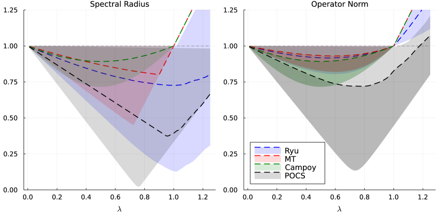
Figure 1: Experiment 1: The median (solid line) and range (shaded region) of the spectral radii and operator norms

For the spectral radius, while Ryu shows a steady decline in the median value for $\lambda<1$, Malitsky-Tam, Campoy, and POCS start increasing well before $\lambda=1$. The maximum value, which can be seen by the range of these values for each algorithm, is some value less than, but close to $1$ for all $\lambda<1$. The operator norm plot, which provides the upper bound for the convergence rates, also stays below 1 for $\lambda<1$. For MT, the sharp edge in the spectral norm appears as the spectral radius involves the maximum of different spectral values. By visual inspection, we see that for Campoy the lower and upper bounds coincide — we weren’t aware of this beforehand and are now able to provide a rigorous proof in Remark 6.1 below.

Remark 6.1.

(relaxed Douglas-Rachford operator) Suppose that $T=T_{\text{\scriptsize C}}$ is the Campoy operator which implies that $T_{\lambda}=(1-\lambda)\operatorname{Id}+\lambda T$ is the relaxed Douglas-Rachford operator for finding a zero of the sum of two normal cone operators of two linear subspaces. By [7, Theorem 3.10(i)], the matrix $T_{\lambda}$ is normal, i.e., $T_{\lambda}T_{\lambda}^{*}=T_{\lambda}^{*}T_{\lambda}$. Moreover, [6, Proposition 3.6(i)] yields $\operatorname{Fix}T=\operatorname{Fix}T_{\lambda}=\operatorname{Fix}T_{\lambda}^{*}=\operatorname{Fix}T^{*}$. Set $P:=P_{\operatorname{Fix}T}=P_{\operatorname{Fix}T^{*}}$ for brevity. Then $P=P^{*}$ and $T_{\lambda}P=P=T_{\lambda}^{*}P$. Taking the transpose yields $PT_{\lambda}^{*}=P=PT_{\lambda}$. Thus

$$(T_{\lambda}-P)(T_{\lambda}-P)^{*} =T_{\lambda}T_{\lambda}^{*}-T_{\lambda}P-PT_{\lambda}^{*}+P$$

$$=T_{\lambda}T_{\lambda}^{*}-P$$

$$=T_{\lambda}^{*}T_{\lambda}-P$$

$$=T_{\lambda}^{*}T_{\lambda}-T_{\lambda}^{*}P-PT_{\lambda}+P$$

$$=(T_{\lambda}-P)^{*}(T_{\lambda}-P),$$

i.e., $T_{\lambda}-P$ is normal as well. Now [19, page 431f] implies that the matrix $T_{\lambda}-P$ is radial, i.e., its spectral radius coincides with its operator norm. This explains that the two (green) curves for the Campoy algorithm in Figure 1 are identical.

6.2 Experiment 2: Number of iterations to achieve prescribed accuracy

Because we know the limit points of the governing as well as shadow sequences, we investigate how varying $\lambda$ affects the number of iterations required to approximate the limit to a given accuracy. For Experiment 2, we fix 100 instances of triples of subspaces $(U_{1},U_{2},U_{3})$. We also fix 100 different starting points in $\mathbb{R}^{6}$. For each instance of the subspaces, starting point $\mathbf{z}_{0}$ and $\lambda\in\{{0.01\cdot k}~{}\big{|}~{}{k\in\{1,2,\ldots,199\}}\}$, we obtain the number of iterations (up to a maximum of $10^{4}$ iterations) required to achieve $\varepsilon=10^{-6}$ accuracy.

For the governing sequence, the limit $P_{\operatorname{Fix}T}(\mathbf{z}_{0})$ is used to determine the stopping condition. Figure 2 reports the median number of iterations required for each $\lambda$ to achieve the given accuracy.

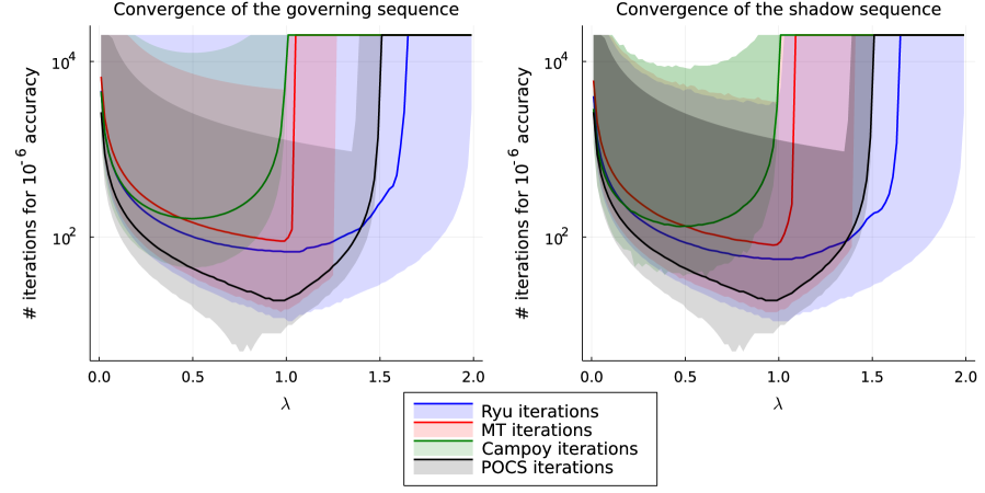
Figure 2: Experiment 2: The median (solid line) and range (shaded region) of the number of iterations for the governing and shadow sequences

For the shadow sequence, we compute the median number of iterations required to achieve $\varepsilon=10^{-6}$ accuracy for the sequence $(\overline{M}\mathbf{z}_{k})_{k\in{\mathbb{N}}}$ with respect to its limit $P_{Z}z_{0}$, where $z_{0}$ is the average of the components of $\mathbf{z}_{0}$. See Figure 2 for results. For POCS, we pick the governing sequence equal to the shadow sequence.

For Ryu and MT in both experiments, increasing values of $\lambda$ result in a decreasing number of median iterations required for $\lambda<1$. For Campoy, the median iterations reach the minimum at $\lambda\approx 0.5$ and keep increasing after that. As is evident from the maximum number of iterations required for a fixed $\lambda$, the shadow sequence converges before the governing sequence for larger values of $\lambda$ in $\left]0,1\right[$. One can also see that Ryu consistently requires fewer median iterations for both the governing and the shadow sequence to achieve the same accuracy as MT for a fixed lambda. However, Campoy performs better than Ryu for small values of $\lambda$, and beats MT for a larger range of $\lambda\in\left]0,0.5\right[$. POCS naturally performed better for all values of $\lambda$. Its behaviour for values of $\lambda$ beyond 1 is similar to Ryu.

6.3 Experiment 3: Convergence plots of shadow sequences

In this experiment, we measure the distance of the terms of the governing (and shadow) sequence from its limit point, to observe how the iterates of the algorithms approach the solution. Guided by Figure 2, we pick the $\lambda$ for which the median iterates are the least: $\lambda=0.99$ for Ryu, $\lambda=0.97$ for MT, and $\lambda=0.57$ for Campoy. Similar to the setup of Experiment 2, we fix 100 starting points and 100 triples of subspaces $(U_{1},U_{2},U_{3})$. We then run the algorithms for 150 iterations for each starting point and each set of subspaces, and we measure the distance of the iterates $\overline{M}\mathbf{z}_{k}$ to its limit $P_{Z}z_{0}$. Figure 3 reports the median of these values for each iteration counter $k\in\{1,\dots,150\}$. Again note that for POCS, the governing sequence coincides with the shadow sequence. As can be seen in Figure 3 for both governing and shadow sequences, Ryu converges faster to the solution compared to MT and Campoy. Ryu and MT show faint “rippling” as is well known to occur for the Douglas-Rachford algorithm. Campoy, already being a DR algorithm, has more prominent ripples. As seen in the previous experiment, POCS outperforms the rest of the algorithms for its optimal value of $\lambda$.

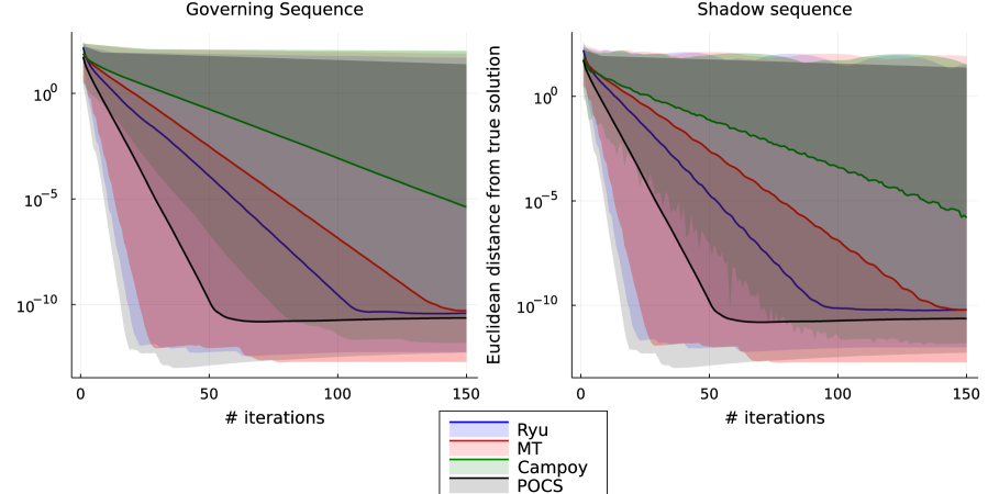
Figure 3: Experiment 3: Convergence plot of the governing and shadow sequences. The median (solid line) and range (shaded region) of distances are reported.

6.4 Discussion

We tested the performance of these algorithms in the specific case of 3 subspaces in $\mathbb{R}^{6}$ through different experiments. The performance of Ryu is better than that of MT and Campoy; however, MT and Campoy have the upper hand when it comes to extending to more subspaces since Ryu is only designed for the 3 subspaces case. Being a sequential algorithm operating solely in the original space (rather than a product space), POCS is faster than the three others in terms of convergence — but the scope of these algorithms is not restricted to projection operators.

7 Three simple lines in the Euclidean plane

In this section, we consider a very simple situation: Three lines passing through the origin, where the second line bisects the angle between the first and the third. We follow the set up in [6, Section 5]. Suppose that $X=\mathbb{R}^{2}$, and set $e_{0}:=[1,0]^{T}$, $e_{\pi/2}:=[0,1]^{T}$, and also

$$e_{\theta}:=\cos(\theta)e_{0}+\sin(\theta)e_{\pi/2}.$$

Define the counterclockwise rotator

$$R_{\theta}:=\begin{bmatrix}\cos(\theta)&-\sin(\theta)\\ \sin(\theta)&\cos(\theta)\end{bmatrix}$$

and now set

$$U:=\mathbb{R}e_{0},\quad V:=\mathbb{R}e_{\theta}=R_{\theta}(U),\quad W:=\mathbb{R}e_{2\theta}=R_{2\theta}(U),$$

where $\theta\in\left]0,\pi/2\right[$. It is clear that $Z=U\cap V\cap W=\{0\}=U\cap V=V\cap W=U\cap W$ and that the Friedrichs angle between $U$ and $V$, and between $V$ and $W$, is $\theta$ while the Friedrichs angle between $U$ and $W$ is $2\theta$. The projectors associated with $U,V,W$ are

$$P_{U} =\begin{bmatrix}1&0\\ 0&0\end{bmatrix},$$

$$P_{V} =\begin{bmatrix}\cos^{2}(\theta)&\sin(\theta)\cos(\theta)\\ \sin(\theta)\cos(\theta)&\sin^{2}(\theta)\end{bmatrix},$$

$$P_{W} =\begin{bmatrix}\cos^{2}(2\theta)&\sin(2\theta)\cos(2\theta)\\ \sin(2\theta)\cos(2\theta)&\sin^{2}(2\theta)\end{bmatrix}.$$

In the next few subsections, we discuss what the relevant splitting operators turn into, while in the last subsection we summarize our findings. The overall strategy is clear: Find a formula for the splitting operator $T$ and then for $\operatorname{Fix}T$. Consider $((1-\lambda)\operatorname{Id}+\lambda T)-P_{\operatorname{Fix}T}$ and determine its largest absolute eigenvalue and its largest spectral value to find the spectral radius and the operator norm. It turns out that this is easier said than done — even with the help of SageMath [28].

7.1 Ryu splitting

The underlying $T=T_{\text{\scriptsize Ryu}}$ (see 59) turns out to be

$$T =\begin{bmatrix}2\cos^{4}(\theta)-\cos^{2}(\theta)&-2\big{(}2\cos^{3}(\theta)-\cos(\theta)\big{)}\sin(\theta)&-2\sin^{4}(\theta)+\sin^{2}(\theta)&-\big{(}2\cos^{3}(\theta)-\cos(\theta)\big{)}\sin(\theta)\\ 2\cos^{3}(\theta)\sin(\theta)&-4\cos^{2}(\theta)\sin^{2}(\theta)+1&2\cos(\theta)\sin^{3}(\theta)&2\cos^{4}(\theta)-2\cos^{2}(\theta)\\ 2\cos^{4}(\theta)-2\cos^{2}(\theta)&-2\big{(}2\cos^{3}(\theta)-\cos(\theta)\big{)}\sin(\theta)&-2\cos^{4}(\theta)+2\cos^{2}(\theta)&-2\cos^{3}(\theta)\sin(\theta)\\ \big{(}2\cos^{3}(\theta)-\cos(\theta)\big{)}\sin(\theta)&-4\cos^{2}(\theta)\sin^{2}(\theta)&-\big{(}2\cos^{3}(\theta)-\cos(\theta)\big{)}\sin(\theta)&2\cos^{4}(\theta)-\cos^{2}(\theta)\end{bmatrix}.$$

Following the procedure of Section 5.1, one eventually arrives at

$$P_{\operatorname{Fix}T}=\begin{bmatrix}0&0&0&0\\ 0&-\frac{1}{4\sin^{2}(\theta)-5}&\frac{2\cos(\theta)\sin(\theta)}{4\cos^{2}(\theta)+1}&-\frac{2\big{(}\cos^{4}(\theta)-\cos^{2}(\theta)\big{)}}{4\sin^{4}(\theta)-5\sin^{2}(\theta)}\\ 0&\frac{2\cos(\theta)\sin(\theta)}{4\cos^{2}(\theta)+1}&\frac{4\big{(}\sin^{4}(\theta)-\sin^{2}(\theta)\big{)}}{4\sin^{2}(\theta)-5}&\frac{4\big{(}\cos^{5}(\theta)-\cos^{3}(\theta)\big{)}}{\big{(}4\cos^{2}(\theta)+1\big{)}\sin(\theta)}\\ 0&-\frac{2\big{(}\cos^{4}(\theta)-\cos^{2}(\theta)\big{)}}{4\sin^{4}(\theta)-5\sin^{2}(\theta)}&\frac{4\big{(}\cos^{5}(\theta)-\cos^{3}(\theta)\big{)}}{\big{(}4\cos^{2}(\theta)+1\big{)}\sin(\theta)}&-\frac{4\cos^{4}(\theta)}{4\sin^{2}(\theta)-5}\end{bmatrix}.$$

Now set $T_{\lambda}:=(1-\lambda)\operatorname{Id}+\lambda T$. We are again interested in the spectral radius and the operator norm of $T_{\lambda}-P_{\operatorname{Fix}T}$ — unfortunately, even with the help of SageMath [28], we were not able to compute these quantities. In fact, even the assignment $\lambda=\tfrac{1}{2}$ did not lead to manageable expressions.

7.2 Malitsky-Tam splitting

Using 66, we find that $T=T_{\text{\scriptsize MT}}$ is

$$T=\begin{bmatrix}0&-\cos(\theta)\sin(\theta)&\cos^{2}(\theta)&\cos(\theta)\sin(\theta)\\ 0&\cos^{2}(\theta)&\cos(\theta)\sin(\theta)&\sin^{2}(\theta)\\ 4\cos^{4}(\theta)-4\cos^{2}(\theta)+1&2\cos(\theta)\sin^{3}(\theta)&0&-2\big{(}2\cos^{3}(\theta)-\cos(\theta)\big{)}\sin(\theta)\\ 2\big{(}2\cos^{3}(\theta)-\cos(\theta)\big{)}\sin(\theta)&2\sin^{4}(\theta)-\sin^{2}(\theta)&0&-4\cos^{2}(\theta)\sin^{2}(\theta)+1\end{bmatrix}.$$

Following the recipe outlined in Section 5.2 yields

$$P_{\operatorname{Fix}T} =\begin{bmatrix}0&0&0&0\\ 0&\tfrac{1}{2}&\cos(\theta)\sin(\theta)&\sin^{2}(\theta)-\tfrac{1}{2}\\ 0&\cos(\theta)\sin(\theta)&-2\sin^{4}(\theta)+2\sin^{2}(\theta)&2\cos(\theta)\sin^{3}(\theta)-\cos(\theta)\sin(\theta)\\ 0&\sin^{2}(\theta)-\tfrac{1}{2}&2\cos(\theta)\sin^{3}(\theta)-\cos(\theta)\sin(\theta)&2\sin^{4}(\theta)-2\sin^{2}(\theta)+\tfrac{1}{2}\end{bmatrix}.$$

Now set $T_{\lambda}:=(1-\lambda)\operatorname{Id}+\lambda T$. We are again interested in the spectral radius and the operator norm of $T_{\lambda}-P_{\operatorname{Fix}T}$. Unfortunately, even with the help of SageMath [28], we were not able to compute eigenvalues or the operator norm, even when we specialized to $\lambda=\tfrac{1}{2}$.

7.3 Campoy splitting

Using 73, we compute the Campoy operator $T=T_{\text{\scriptsize C}}$ to be

$$T=\begin{bmatrix}-\sin^{2}(2\theta)&\sin(2\theta)\cos(2\theta)&\cos^{2}(2\theta)&\sin(2\theta)\cos(2\theta)\\ -\sin(2\theta)\cos(2\theta)&\cos^{2}(2\theta)&-\sin(2\theta)\cos(2\theta)&-\sin^{2}(2\theta)\\ \cos(2\theta)&\sin(2\theta)&0&0\\ 0&0&-\sin(2\theta)&\cos(2\theta)\end{bmatrix}.$$

The operator $T$ is actually an isometry (as can be checked directly or after applying [8, Proposition 3.5]); unfortunately, we could not determine $P_{\operatorname{Fix}T}$ because the computation of the symbolic computation of Moore-Penrose inverses in 75 turned out to be too complicated even when using SageMath [28].

7.4 POCS

The method of Projections onto Convex Sets (POCS) is known to converge to the projection onto the intersection when applied to linear subspaces. In contrast to the parallel splitting methods discussed above, POCS is sequential in nature not requiring any product space. First, we note that

$$P_{W}P_{V}P_{U} =\begin{bmatrix}2\cos^{4}(\theta)-\cos^{2}(\theta)&0\\ 2\cos^{3}(\theta)\sin(\theta)&0\end{bmatrix}=\cos^{2}(\theta)\begin{bmatrix}2\cos^{2}(\theta)-1&0\\ 2\cos(\theta)\sin(\theta)&0\end{bmatrix}$$

$$=\cos^{2}(\theta)\begin{bmatrix}\cos(2\theta)&0\\ \sin(2\theta)&0\end{bmatrix}.$$

Next, the reflected POCS operator $T$ (see 76) simplifies to

$$T :=\tfrac{4}{3}P_{W}P_{V}P_{U}-\tfrac{1}{3}\operatorname{Id}=\tfrac{1}{3}\begin{bmatrix}{8}\cos^{4}({\theta})-{4}\cos^{2}({\theta})-{1}&0\\ {8}\cos^{3}({\theta})\sin({\theta})&-{1}\end{bmatrix}.$$

Note that $\operatorname{Fix}T=\{0\}$ and hence $P_{\operatorname{Fix}T}=0$. Thus Next, we set as before $T_{\lambda}:=(1-\lambda)\operatorname{Id}+\lambda T$; hence,

$$T_{\lambda}-P_{\operatorname{Fix}T}=(1-\lambda)\operatorname{Id}+\lambda T.$$

After simplification, the two eigenvalues of $T_{\lambda}-P_{\operatorname{Fix}T}=T_{\lambda}$ are seen to be real and equal to $1-\tfrac{4}{3}\lambda$ and $1+\tfrac{4}{3}\lambda\big{(}2\sin^{4}(\theta)-3\sin^{2}(\theta))$. It follows that the spectral radius of $T_{\lambda}-P_{\operatorname{Fix}T}$ is equal to

$$\max\big{\{}\big{|}1-\tfrac{4}{3}\lambda\big{|},\big{|}1+\tfrac{4}{3}\lambda\big{(}2\sin^{4}(\theta)-3\sin^{2}(\theta)\big{)}\big{|}\big{\}}.$$

The eigenvalues of $(T_{\lambda}-P_{\operatorname{Fix}T})^{*}(T_{\lambda}-P_{\operatorname{Fix}T})=T_{\lambda}^{*}T_{\lambda}$ are available but too complicated to list here. To make progress analytically, we assume that

$$\lambda=\tfrac{4}{3},$$

i.e., we consider the original POCS operator $P_{W}P_{V}P_{U}$. The spectral radius of $T_{\lambda}-P_{\operatorname{Fix}T}$ simplifies then to

$$1+2\sin^{4}(\theta)-3\sin^{2}(\theta)=\cos^{2}(\theta)\cos(2\theta)$$

while the operator norm of $T_{\lambda}-P_{\operatorname{Fix}T}$ is

$$\cos^{2}(\theta).$$

7.5 Discussion

It is tempting to ask whether the splitting methods by Ryu, by Malitksy-Tam, and by Campoy allow a complete analysis like the one available for Douglas–Rachford splitting for two subspaces as carried out in [6]. Unfortunately, a symbolic analysis of these methods seems much harder even for the shockingly simple case considered in this section. Thus at present, we are rather pessimistic about the prospect of obtaining pleasant convergence rate for this new breed of splitting methods — but we hope that the reader will prove us wrong!

8 Conclusion

In this paper, we investigated the recent splitting methods by Ryu, by Malitsky-Tam, and by Campoy in the context of normal cone operators for subspaces. We discovered and proved that all three algorithms find not just some solution but in fact the projection of the starting point onto the intersection of the subspaces. Moreover, convergence of the iterates is strong even in infinite-dimensional settings. Our numerical experiments illustrated that Ryu’s method seems to converge faster although neither Malitsky-Tam splitting nor Campoy splitting is limited in its applicability to just 3 subspaces.

Two natural avenues for future research are the following. Firstly, when $X$ is finite-dimensional, we know that the convergence rate of the iterates is linear. While we illustrated this linear convergence numerically in this paper, it is open whether there are natural bounds for the linear rates in terms of some version of angle between the subspaces involved. For the prototypical Douglas-Rachford splitting framework, this was carried out in [6] and [7] in terms of the Friedrichs angle. Secondly, what can be said in the inconsistent affine case? Again, the Douglas-Rachford algorithm may serve as a guide to what the expected results and complications might be; see, e.g., [11]. However, these topics for further research appear to be quite hard.

References

- [1] W.N. Anderson and R.J. Duffin, Series and parallel addition of matrices, Journal of Mathematical Analysis and Applications 26, 576–594, 1969. https://doi.org/10.1016/0022-247X(69)90200-5
- [2] F.J. Aragón-Artacho, R. Campoy, and M.K. Tam, Strengthened splitting methods for computing resolvents, Computational Optimization and Applications 80, 549–585, 2021. https://doi.org/10.1007/s10589-021-00291-6
- [3] C. Badea, S. Grivaux, and V. Müller, The rate of convergence in the method of alternating projections, St. Petersburg Mathematical Journal 23(3), 413–434, 2011. https://doi.org/10.1090/S1061-0022-2012-01202-1
- [4] J.B. Baillon, Quelques propriétés de convergence asymptotique pour les contractions impaires, Comptes rendus de l’Académie des Sciences 238, Aii, A587–A590, 1976.
- [5] J.B. Baillon, R.E. Bruck, and S. Reich, On the asymptotic behavior of nonexpansive mappings and semigroups in Banach spaces, Houston Journal of Mathematics 4(1), 1–9, 1978. https://www.math.uh.edu/~hjm/restricted/archive/v004n1/0001BAILLON.pdf
- [6] H.H. Bauschke, J.Y. Bello Cruz, T.T.A. Nghia, H.M. Phan, and X. Wang, The rate of linear convergence of the Douglas-Rachford algorithm for subspaces is the cosine of the Friedrichs angle, Journal of Approximation Theory 185, 63–79, 2014. https://doi.org/10.1016/j.jat.2014.06.002
- [7] H.H. Bauschke, J.Y. Bello Cruz, T.T.A. Nghia, H.M. Phan, and X. Wang, Optimal rates of linear convergence of relaxed alternating projections and generalized Douglas-Rachford methods for two subspaces, Numerical Algorithms 73, 33–76, 2016. https://doi.org/10.1007/s11075-015-0085-4
- [8] H.H. Bauschke and P.L. Combettes, Convex Analysis and Monotone Operator Theory in Hilbert Spaces, second edition, Springer, 2017. https://doi.org/10.1007/978-3-319-48311-5
- [9] H.H. Bauschke, F. Deutsch, H. Hundal, and S.-H. Park, Accelerating the convergence of the method of alternating projections, Transactions of the AMS 355(9), 3433–3461, 2003. https://doi.org/10.1090/S0002-9947-03-03136-2
- [10] H.H. Bauschke, B. Lukens, and W.M. Moursi, Affine nonexpansive operators, Attouch-Théra duality, and the Douglas-Rachford algorithm, Set-Valued and Variational Analysis 25, 481–505, 2017. https://doi.org/10.1007/s11228-016-0399-y
- [11] H.H. Bauschke and W.M. Moursi, The Douglas-Rachford algorithm for two (not necessarily intersecting) affine subspaces, SIAM Journal on Optimization 26(2), 968–985, 2016. https://doi.org/10.1137/15M1016989
- [12] J. Bezanson, A. Edelman, S. Karpinski, and V.B. Shah, Julia: a fresh approach to numerical computing, SIAM Review 59(1), 65–98, 2017. https://doi.org/10.1137/141000671
- [13] L.M. Briceño-Arias, Resolvent splitting with minimal lifting for composite monotone inclusions. https://arxiv.org/abs/2111.09757v2
- [14] R.E. Bruck and S. Reich, Nonexpansive projections and resolvents of accretive operators in Banach spaces, Houston Journal of Mathematics 3(4), 459–470, 1977. https://www.math.uh.edu/~hjm/restricted/archive/v003n4/0459BRUCK.pdf
- [15] R. Campoy, A product space reformulation with reduced dimension for splitting algorithms, Computational Optimization and Applications 83, 319–348, 2022. https://doi.org/10.1007/s10589-022-00395-7
- [16] P.L. Combettes, Iterative construction of the resolvent of a sum of maximal monotone operators, Journal of Convex Analysis 16(4), 727–748, 2009. https://www.heldermann.de/JCA/JCA16/JCA163/jca16044.htm
- [17] F. Deutsch, Best Approximation in Inner Product Spaces, Springer, 2001. https://doi.org/10.1007/978-1-4684-9298-9
- [18] J. Douglas and H.H. Rachford, On the numerical solution of heat conduction problems in two and three space variables, Transactions of the AMS 82, 421–439, 1956. https://doi.org/10.1090/S0002-9947-1956-0084194-4
- [19] M. Goldberg and G. Zwas, On matrices having equal spectral radius and spectral norm, Linear Algebra and its Applications 8, 427–434, 1974. https://doi.org/10.1016/0024-3795(74)90076-7
- [20] C.W. Groetsch, Generalized Inverses of Linear Operators, Marcel Dekker, 1977.
- [21] S. Kayalar and H.L. Weinert, Error bounds for the method of alternating projections, Mathematics of Control, Signals, and Systems 1, 43–59, 1988. https://doi.org/10.1007/BF02551235
- [22] A.Y. Kruger, Generalized differentials of nonsmooth functions, 1981, Minsk. Deposited in VINITI no. 1332-81. Available from https://asterius.federation.edu.au/akruger/research/publications.html as https://asterius.federation.edu.au/akruger/research/papers/1332-81.pdf.
- [23] A.Y. Kruger, Generalized differentials of nonsmooth functions, and necessary conditions for an extremum, Siberian Mathematics Journal 26, 370–379, 1985. https://doi.org/10.1007/BF00968624. Available from https://asterius.federation.edu.au/akruger/research/publications.html as https://asterius.federation.edu.au/akruger/research/papers/1985_SMJ3.pdf.
- [24] P.-L. Lions and B. Mercier, Splitting algorithms for the sum of two nonlinear operators, SIAM Journal on Numerical Analysis 16, 964–979, 1979. https://doi.org/10.1137/0716071
- [25] Y. Malitsky and M.K. Tam, Resolvent splitting for sums of monotone operators with minimal lifting. https://arxiv.org/abs/2108.02897v2
- [26] C.D. Meyer, Matrix Analysis and Applied Linear Algebra, SIAM, 2000.
- [27] E.K. Ryu, Uniqueness of DRS as the 2 operator resolvent-splitting and impossibility of 3 operator resolvent-splitting, Mathematical Programming (Series A) 182, 233–273, 2020. https://doi.org/10.1007/s10107-019-01403-1
- [28] The Sage Developers, SageMath, https:www.sagemath.org, 2022.