Incorporating Hierarchy into Text Encoder: a Contrastive Learning Approach for Hierarchical Text Classification

Abstract

Hierarchical text classification is a challenging subtask of multi-label classification due to its complex label hierarchy. Existing methods encode text and label hierarchy separately and mix their representations for classification, where the hierarchy remains unchanged for all input text. Instead of modeling them separately, in this work, we propose Hierarchy-guided Contrastive Learning (HGCLR) to directly embed the hierarchy into a text encoder. During training, HGCLR constructs positive samples for input text under the guidance of the label hierarchy. By pulling together the input text and its positive sample, the text encoder can learn to generate the hierarchy-aware text representation independently. Therefore, after training, the HGCLR enhanced text encoder can dispense with the redundant hierarchy. Extensive experiments on three benchmark datasets verify the effectiveness of HGCLR.

1 Introduction

Hierarchical Text Classification (HTC) aims to categorize text into a set of labels that are organized in a structured hierarchy Silla and Freitas (2011). The taxonomic hierarchy is commonly modeled as a tree or a directed acyclic graph, in which each node is a label to be classified. As a subtask of multi-label classification, the key challenge of HTC is how to model the large-scale, imbalanced, and structured label hierarchy Mao et al. (2019).

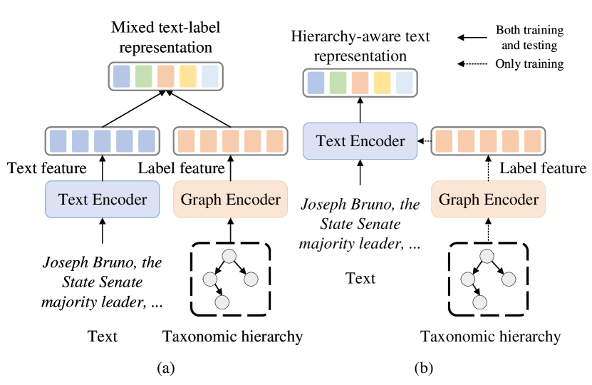
Figure 1: Two ways of introducing hierarchy information. (a) Previous work model text and labels separately and find a mixed representation. (b) Our method incorporating hierarchy information into text encoder for a hierarchy-aware text representation.

The existing methods of HTC have variously introduced hierarchical information. Among recent researches, the state-of-the-art models encode text and label hierarchy separately and aggregate two representations before being classified by a mixed feature Zhou et al. (2020); Deng et al. (2021). As denoted in the left part of Figure 1, their main goal is to sufficiently interact between text and structure to achieve a mixed representation Chen et al. (2021), which is highly useful for classification Chen et al. (2020a). However, since the label hierarchy remains unchanged for all text inputs, the graph encoder provides exactly the same representation regardless of the input. Therefore, the text representation interacts with constant hierarchy representation and thus the interaction seems redundant and less effective. Alternatively, we attempt to inject the constant hierarchy representation into the text encoder. So that after being fully trained, a hierarchy-aware text representation can be acquired without the constant label feature. As in the right part of Figure 1, instead of modeling text and labels separately, migrating label hierarchy into text encoding may benefit HTC by a proper representation learning method.

To this end, we adopt contrastive learning for the hierarchy-aware representation. Contrastive learning, which aims to concentrate positive samples and push apart negative samples, has been considered as effective in constructing meaningful representations Kim et al. (2021). Previous work on contrastive learning illustrates that it is critical to building challenging samples Alzantot et al. (2018); Wang et al. (2021b); Tan et al. (2020); Wu et al. (2020). For multi-label classification, we attempt to construct high-quality positive examples. Existing methods for positive example generation includes data augmentation Meng et al. (2021); Wu et al. (2020), dropout Gao et al. (2021), and adversarial attack Wang et al. (2021b); Pan et al. (2021). These techniques are either unsupervised or task-unspecific: the generation of positive samples has no relation with the HTC task and thus are incompetent to acquire hierarchy-aware representations. As mentioned, we argue that both the ground-truth label as well as the taxonomic hierarchy should be considered for the HTC task.

To construct positive samples which are both label-guided and hierarchy-involved, our approach is motivated by a preliminary observation. Notice that when we classify text into a certain category, most words or tokens are not important. For instance, when a paragraph of news report about a lately sports match is classified as “basketball”, few keywords like “NBA” or “backboard” have large impacts while the game result has less influence. So, given a sequence and its labels, a shorten sequence that only keeps few keywords should maintain the labels. In fact, this idea is similar to adversarial attack, which aims to find “important tokens” which affect classification most Zhang et al. (2020). The difference is that adversarial attack tries to modify “important tokens” to fool the model, whereas our approach modifies “unimportant tokens” to keep the classification result unchanged.

Under such observation, we construct positive samples as pairs of input sequences and theirs shorten counterparts, and propose Hierarchy-Guided Contrastive Learning (HGCLR) for HTC. In order to locate keywords under given labels, we directly calculate the attention weight of each token embedding on each label, and tokens with weight above a threshold are considered important to according label. We use a graph encoder to encode label hierarchy and output label features. Unlike previous studies with GCN or GAT, we modify a Graphormer Ying et al. (2021) as our graph encoder. Graphormer encodes graphs by Transformer blocks and outperforms other graph encoders on several graph-related tasks. It models the graph from multiple dimensions, which can be customized easily for HTC task.

The main contribution of our work can be summarized as follows:

• We propose Hierarchy-Guided Contrastive Learning (HGCLR) to obtain hierarchy-aware text representation for HTC. To our knowledge, this is the first work that adopts contrastive learning on HTC.

• For contrastive learning, we construct positive samples by a novel approach guided by label hierarchy. The model employs a modified Graphormer, which is a new state-of-the-art graph encoder.

• Experiments demonstrate that the proposed model achieves improvements on three datasets. Our code is available at https://github.com/wzh9969/contrastive-htc.

2 Related Work

2.1 Hierarchical Text Classification

Existing work for HTC could be categorized into local and global approaches based on their ways of treating the label hierarchy Zhou et al. (2020). Local approaches build classifiers for each node or level while the global ones build only one classifier for the entire graph. Banerjee et al. (2019) builds one classifier per label and transfers parameters of the parent model for child models. Wehrmann et al. (2018) proposes a hybrid model combining local and global optimizations. Shimura et al. (2018) applies CNN to utilize the data in the upper levels to contribute categorization in the lower levels.

The early global approaches neglect the hierarchical structure of labels and view the problem as a flat multi-label classification Johnson and Zhang (2015). Later on, some work tries to coalesce the label structure by recursive regularization Gopal and Yang (2013), reinforcement learning Mao et al. (2019), capsule network Peng et al. (2019), and meta-learning Wu et al. (2019). Although such methods can capture the hierarchical information, recent researches demonstrate that encoding the holistic label structure directly by a structure encoder can further improve performance. Zhou et al. (2020) designs a structure encoder that integrates the label prior hierarchy knowledge to learn label representations. Chen et al. (2020a) embeds word and label hierarchies jointly in the hyperbolic space. Zhang et al. (2021) extracts text features according to different hierarchy levels. Deng et al. (2021) introduces information maximization to constrain label representation learning. Zhao et al. (2021) designs a self-adaption fusion strategy to extract features from text and label. Chen et al. (2021) views the problem as semantic matching and tries BERT as text encoder. Wang et al. (2021a) proposes a cognitive structure learning model for HTC. Similar to other work, they model text and label separately.

2.2 Contrastive Learning

Contrastive learning is originally proposed in Computer Vision (CV) as a weak-supervised representation learning method. Works such as MoCo He et al. (2020) and SimCLR Chen et al. (2020b) have bridged the gap between self-supervised learning and supervised learning on multiple CV datasets. A key component for applying contrastive learning on NLP is how to build positive pairs Pan et al. (2021). Data augmentation techniques such as back-translation Fang et al. (2020), word or span permutation Wu et al. (2020), and random masking Meng et al. (2021) can generate pair of data with similar meanings. Gao et al. (2021) uses different dropout masks on the same data to generate positive pairs. Kim et al. (2021) utilizes BERT representation by a fixed copy of BERT. These methods do not rely on downstream tasks while some researchers leverage supervised information for better performance on text classification. Wang et al. (2021b) constructs both positive and negative pairs especially for sentimental classification by word replacement. Pan et al. (2021) proposes to regularize Transformer-based encoders for text classification tasks by FGSM Goodfellow et al. (2014), an adversarial attack method based on gradient. Though methods above are designed for classification, the construction of positive samples hardly relies on their categories, neglecting the connection and diversity between different labels. For HTC, the taxonomic hierarchy models the relation between labels, which we believe can help positive sample generation.

3 Problem Definition

Given a input text $x=\{x_{1},x_{2},...,x_{n}\}$, Hierarchical Text Classification (HTC) aims to predict a subset $y$ of label set $Y$, where $n$ is the length of the input sequence and $k$ is the size of set $Y$. The candidate labels $y_{i}\in Y$ are predefined and organized as a Directed Acyclic Graph (DAG) $G=(Y,E)$, where node set $Y$ are labels and edge set $E$ denotes their hierarchy. For simplicity, we do not distinguish a label with its node in the hierarchy so that $y_{i}$ is both a label and a node. Since a non-root label of HTC has one and only one father, the taxonomic hierarchy can be converted to a tree-like hierarchy. The subset $y$ corresponds to one or more paths in $G$: for any non-root label $y_{j}\in y$, a father node (label) of $y_{j}$ is in the subset $y$.

4 Methodology

In this section, we will describe the proposed HGCLR in detail. Figure 2 shows the overall architecture of the model.

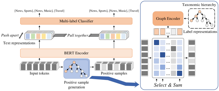
Figure 2: An overview of HGCLR under a batch of 3. HGCLR adopts a contrastive learning framework to regularize BERT representations. We construct positive samples by masking unimportant tokens under the guidance of hierarchy and labels. By pulling together and pushing apart representations, the hierarchy information can be injected into the BERT encoder.

4.1 Text Encoder

Our approach needs a strong text encoder for hierarchy injection, so we choose BERT Devlin et al. (2019) as the text encoder. Given an input token sequence:

$$x=\{{\rm[CLS]},x_{1},x_{2},...,x_{n-2},{\rm[SEP]}\}$$ (1)

where $\rm[CLS]$ and $\rm[SEP]$ are two special tokens indicating the beginning and the end of the sequence, the input is fed into BERT. For convenience, we denote the length of the sequence as $n$. The text encoder outputs hidden representation for each token:

$$H=\rm{BERT}(x)$$ (2)

where $H\in\mathbb{R}^{n\times d_{h}}$ and $d_{h}$ is the hidden size. We use the hidden state of the first token ($\rm[CLS]$) for representing the whole sequence $h_{x}=h_{\rm[CLS]}$.

4.2 Graph Encoder

We model the label hierarchy with a customized Graphormer Ying et al. (2021). Graphormer models graphs on the base of Transformer layer Vaswani et al. (2017) with spatial encoding and edge encoding, so it can leverage the most powerful sequential modeling network in the graph domain. We organize the original feature for node $y_{i}$ as the sum of label embedding and its name embedding:

$$f_{i}={\rm label\_emb}(y_{i})+{\rm name\_emb}(y_{i}).$$ (3)

Label embedding is a learnable embedding that takes a label as input and outputs a vector with size $d_{h}$. Name embedding takes the advantage of the name of the label, which we believe contains fruitful information as a summary of the entire class. We use the average of BERT token embedding of the label as its name embedding, which also has a size of $d_{h}$. Unlike previous work which only adopts names on initialization, we share embedding weights across text and labels to make label features more instructive. With all node features stack as a matrix $F\in\mathbb{R}^{k\times d_{h}}$, a standard self-attention layer can then be used for feature migration.

To leverage the structural information, spatial encoding and edge encoding modify the Query-Key product matrix $A^{G}$ in the self-attention layer:

$$A^{G}_{ij}=\frac{(f_{i}W_{Q}^{G})(f_{j}W_{K}^{G})^{T}}{\sqrt{d_{h}}}+c_{ij}+b_{\phi(y_{i},y_{j})}$$ (4)

where $c_{ij}=\frac{1}{D}\sum_{n=1}^{D}w_{e_{n}}$ and $D=\phi(y_{i},y_{j})$. The first term in Equation 4 is the standard scale-dot attention, and query and key are projected by $W_{Q}^{G}\in\mathbb{R}^{d_{h}\times d_{h}}$ and $W_{K}^{G}\in\mathbb{R}^{d_{h}\times d_{h}}$. $c_{ij}$ is the edge encoding and $\phi(y_{i},y_{j})$ denotes the distance between two nodes $y_{i}$ and $y_{j}$. Since the graph is a tree in our problem, for node $y_{i}$ and $y_{j}$, one and only one path $(e_{1},e_{2},...,e_{D})$ can be found between them in the underlying graph $G^{\prime}$ so that $c_{ij}$ denotes the edge information between two nodes and $w_{e_{i}}\in\mathbb{R}^{1}$ is a learnable weight for each edge. $b_{\phi(y_{i},y_{j})}$ is the spatial encoding, which measures the connectivity between two nodes. It is a learnable scalar indexed by $\phi(y_{i},y_{j})$.

The graph-involved attention weight matrix $A^{G}$ is then followed by Softmax, multiplying with value matrix and residual connection & layer normalization to calculate the self-attention,

$$L=\rm LayerNorm({\rm softmax}(A^{G})V+F)$$ (5)

We use $L$ as the label feature for the next step. The Graphormer we use is a variant of the self-attention layer, for more details on the full structure of Graphormer, please refer to the original paper.

4.3 Positive Sample Generation

As mentioned, the goal for the positive sample generation is to keep a fraction of tokens while retaining the labels. Given a token sequence as Equation 1, the token embedding of BERT is defined as:

$$\{e_{1},e_{2},...,e_{n}\}={\rm BERT\_emb}(x)$$ (6)

The scale-dot attention weight between token embedding and label feature is first calculated to determine the importance of a token on a label,

$$q_{i}=e_{i}W_{Q},k_{j}=l_{j}W_{K},A_{ij}=\frac{q_{i}k_{j}^{T}}{\sqrt{d_{h}}}$$ (7)

The query and key are token embeddings and label features respectively, and $W_{Q}\in\mathbb{R}^{d_{h}\times d_{h}}$ and $W_{K}\in\mathbb{R}^{d_{h}\times d_{h}}$ are two weight matrices. Thus, for a certain $x_{i}$, its probability of belonging to label $y_{j}$ can be normalized by a Softmax function.

Next, given a label $y_{j}$, we can sample key tokens from that distribution and form a positive sample $\hat{x}$. To make the sampling differentiable, we replace the Softmax function with Gumbel-Softmax Jang et al. (2016) to simulate the sampling operation:

$$P_{ij}={\rm gumbel\_softmax}(A_{i1},A_{i2},...,A_{ik})_{j}$$ (8)

Notice that a token can impact more than one label, so we do not discretize the probability as one-hot vectors in this step. Instead, we keep tokens for positive examples if their probabilities of being sampled exceed a certain threshold $\gamma$, which can also control the fraction of tokens to be retrained. For multi-label classification, we simply add the probabilities of all ground-truth labels and obtain the probability of a token $x_{i}$ regarding its ground-truth label set $y$ as:

$$P_{i}=\sum_{j\in y}P_{ij}$$ (9)

Finally, the positive sample $\hat{x}$ is constructed as:

$$\hat{x}=\{x_{i}\text{ if }P_{i}>\gamma\text{ else }\mathbf{0}\}$$ (10)

where $\mathbf{0}$ is a special token that has an embedding of all zeros so that key tokens can keep their positions. The select operation is not differentiable, so we implement it differently to make sure the whole model can be trained end-to-end. Details are illustrated in Appendix A.

The positive sample is fed to the same BERT as the original one,

$$\hat{H}={\rm BERT}(\hat{x})$$ (11)

and get a sequence representation $\hat{h_{x}}$ with the first token before being classified. We assume the positive sample should retain the labels, so we use classification loss of the positive sample as a guidance of the graph encoder and the positive sample generation.

4.4 Contrastive Learning Module

Intuitively, given a pair of token sequences and their positive counterpart, their encoded sentence-level representation should be as similar to each other as possible. Meanwhile, examples not from the same pair should be farther away in the representation space.

Concretely, with a batch of $N$ hidden state of positive pairs $(h_{i},\hat{h_{i}})$, we add a non-linear layer on top of them:

$$c_{i}=W_{2}{\rm ReLU}(W_{1}h_{i})$$ (12)

$$\hat{c_{i}}=W_{2}{\rm ReLU}(W_{1}\hat{h_{i}})$$

where $W_{1}\in\mathrm{R}^{d_{h}\times d_{h}}$, $W_{2}\in\mathrm{R}^{d_{h}\times d_{h}}$. For each example, there are $2(N-1)$ negative pairs, i.e., all the remaining examples in the batch are negative examples. Thus, for a batch of $2N$ examples $\mathbf{Z}=\{z\in\{c_{i}\}\cup\{\hat{c_{i}}\}\}$, we compute the NT-Xent loss Chen et al. (2020b) for $z_{m}$ as:

$$L_{m}^{con}=-\log\frac{\exp({\rm sim}(z_{m},\mu(z_{m}))/\tau)}{\sum^{2N}_{i=1,i\not=m}\exp({\rm sim}(z_{m},z_{i})/\tau)}$$ (13)

where $\rm sim$ is the cosine similarity function as ${\rm sim}(u,v)=u\cdot v/\|u\|\|v\|$ and $\mu$ is a matching function as:

$$\mu(z_{m})=\left\{\begin{array}[]{ll}c_{i},\text{ if }z_{m}=\hat{c_{i}}&\\ \hat{c_{i}},\text{ if }z_{m}=c_{i}&\end{array}\right.$$ (14)

$\tau$ is a temperature hyperparameter.

The total contrastive loss is the mean loss of all examples:

$$L^{con}=\frac{1}{2N}\sum_{m=1}^{2N}L_{m}^{con}$$ (15)

4.5 Classification and Objective Function

Following previous work Zhou et al. (2020), we flatten the hierarchy for multi-label classification. The hidden feature is fed into a linear layer, and a sigmoid function is used for calculating the probability. The probability of text $i$ on label $j$ is:

$$p_{ij}={\rm sigmoid}(W_{c}h_{i}+b_{c})_{j}$$ (16)

where $W_{C}\in\mathbb{R}^{k\times d_{h}}$ and $b_{c}\in\mathbb{R}^{k}$ are weights and bias. For multi-label classification, we use a binary cross-entropy loss function for text $i$ on label $j$,

$$L_{ij}^{C}=-y_{ij}\log(p_{ij})-(1-y_{ij})\log(1-p_{ij})$$ (17)

$$L^{C}=\sum_{i=1}^{N}\sum_{j=1}^{k}L_{ij}^{C}$$ (18)

where $y_{ij}$ is the ground truth. The classification loss of the constructed positive examples $\hat{L^{C}}$ can be calculated similarly by Equation 16 and Equation 18 with $\hat{h_{i}}$ substituting for $h_{i}$.

The final loss function is the combination of classification loss of original data, classification loss of the constructed positive samples, and the contrastive learning loss:

$$L=L^{C}+\hat{L^{C}}+\lambda L^{con}$$ (19)

where $\lambda$ is a hyperparameter controlling the weight of contrastive loss.

During testing, we only use the text encoder for classification and the model degenerates to a BERT encoder with a classification head.

Dataset	$|Y|$	Depth	Avg($|y_{i}|$)	Train	Dev	Test
WOS	141	2	2.0	30,070	7,518	9,397
NYT	166	8	7.6	23,345	5,834	7,292
RCV1-V2	103	4	3.24	20,833	2,316	781,265

Table 1: Data Statistics. $|Y|$ is the number of classes. Depth is the maximum level of hierarchy. Avg($|y_{i}|$) is the average number of classes per sample.

Model	WOS		NYT		RCV1-V2
	Micro-F1	Macro-F1	Micro-F1	Macro-F1	Micro-F1	Macro-F1
Hierarchy-Aware Models
TextRCNN Zhou et al. (2020)	83.55	76.99	70.83	56.18	81.57	59.25
HiAGM Zhou et al. (2020)	85.82	80.28	74.97	60.83	83.96	63.35
HTCInfoMax Deng et al. (2021)	85.58	80.05	-	-	83.51	62.71
HiMatch Chen et al. (2021)	86.20	80.53	-	-	84.73	64.11
Pretrained Language Models
BERT (Our implement)	85.63	79.07	78.24	65.62	85.65	67.02
BERT Chen et al. (2021)	86.26	80.58	-	-	86.26	67.35
BERT+HiAGM (Our implement)	86.04	80.19	78.64	66.76	85.58	67.93
BERT+HTCInfoMax (Our implement)	86.30	79.97	78.75	67.31	85.53	67.09
BERT+HiMatch Chen et al. (2021)	86.70	81.06	-	-	86.33	68.66
HGCLR	87.11	81.20	78.86	67.96	86.49	68.31

Table 2: Experimental results of our proposed model on several datasets. For a fair comparison, we implement some baseline with BERT encoder. We cannot reproduce the BERT results reported in Chen et al. (2021) so that we also report the results of our version of BERT.

5 Experiments

5.1 Experiment Setup

Datasets and Evaluation Metrics

We experiment on Web-of-Science (WOS) Kowsari et al. (2017), NYTimes (NYT) Sandhaus (2008), and RCV1-V2 Lewis et al. (2004) datasets for comparison and analysis. WOS contains abstracts of published papers from Web of Science while NYT and RCV1-V2 are both news categorization corpora. We follow the data processing of previous work Zhou et al. (2020). WOS is for single-path HTC while NYT and RCV1-V2 include multi-path taxonomic labels. The statistic details are illustrated in Table 1. Similar to previous work, We measure the experimental results with Macro-F1 and Micro-F1.

Implement Details

For text encoder, we use bert-base-uncased from Transformers Wolf et al. (2020) as the base architecture. Notice that we denote the attention layer in Eq. 4 and Eq. 7 as single-head attentions but they can be extended to multi-head attentions as the original Transformer block. For Graphormer, we set the attention head to $8$ and feature size $d_{h}$ to $768$. The batch size is set to $12$. The optimizer is Adam with a learning rate of $3e-5$. We implement our model in PyTorch and train end-to-end. We train the model with train set and evaluate on development set after every epoch, and stop training if the Macro-F1 does not increase for $6$ epochs. The threshold $\gamma$ is set to $0.02$ on WOS and $0.005$ on NYT and RCV1-V2. The loss weight $\lambda$ is set to $0.1$ on WOS and RCV1-V2 and $0.3$ on NYT. $\gamma$ and $\lambda$ are selected by grid search on development set. The temperature of contrastive module is fixed to $1$ since we have achieved promising results with this default setting in preliminary experiments.

Baselines

We select a few recent work as baselines. HiAGM Zhou et al. (2020), HTCInfoMax Deng et al. (2021), and HiMatch Chen et al. (2021) are a branch of work that propose fusion strategies for mixed text-hierarchy representation. HiAGM applies soft attention over text feature and label feature for the mixed feature. HTCInfoMax improves HiAGM by regularizing the label representation with a prior distribution. HiMatch matches text representation with label representation in a joint embedding space and uses joint representation for classification. HiMatch is the state-of-the-art before our work. All approaches except HiMatch adopt TextRCNN Lai et al. (2015) as text encoder so that we implement them with BERT for a fair comparison.

5.2 Experimental Results

Main results are shown in Table 2. Instead of modeling text and labels separately, our model can make more use of the strong text encoder by migrating hierarchy information directly into BERT encoder. On WOS, the proposed HGCLR can achieve 1.5% and 2.1% improvement on Micro-F1 and Macro-F1 respectively comparing to BERT and is better than HiMatch even if its base model has far better performance.

BERT was trained on news corpus so that the base model already has decent performance on NYT and RCV1-V2, outperforming post-pretrain models by a large amount. On NYT, our approach observes a 2.3% boost on Macro-F1 comparing to BERT while sightly increases on Micro-F1 and outperform previous methods on both measurements.

On RCV1-V2, all baselines hardly improve Micro-F1 and only influence Macro-F1 comparing to BERT. HTCInfoMax experiences a decrease because its constraint on text representation may contradict with BERT on this dataset. HiMatch behaves extremely well on RCV1-V2 with Macro-F1 as measurement while our approach achieves state-of-the-art on Micro-F1. Besides the potential implement difference on BERT encoder, RCV1-V2 dataset provides no label name, which invalids our name embedding for label representation. Baselines like HiAGM and HiMatch only initialize labl embedding with their names so that this flaw has less impact. We will discuss more on name embedding in next section.

5.3 Analysis

Ablation Models	Micro-F1	Macro-F1
BERT	85.75	79.36
HGCLR	87.46	81.52
-r.p. GCN	87.06	80.63
-r.p. GAT	87.18	81.45
-r.m. graph encoder	86.67	80.11
-r.m. contrastive loss	86.72	80.97

Table 3: Performance when replace or remove some components of HGCLR on the development set of WOS. r.p. stands for replace and r.m. stands for remove. We remove the contrastive loss by setting $\lambda=0$.

The main differences between our work and previous ones are the graph encoder and contrastive learning. To illustrate the effectiveness of these two parts, we test our model with them replaced or removed. We report the results on the development set of WOS for illustration. We first replace Graphormer with GCN and GAT (r.p. GCN and r.p. GAT), results are in Table 3. We find that Graphormer outperforms both graph encoders on this task. GAT also involves the attention mechanism but a node can only attend to its neighbors. Graphormer adopts global attention where each node can attend to all others in the graph, which is proven empirically more effective on this task. When the graph encoder is removed entirely (-r.m. graph encoder), the results drop significantly, showing the necessity of incorporating graph encoder for HTC task.

The model without contrastive loss is similar to a pure data augmentation approach, where positive examples stand as augment data. As the last row of Table 3, on development set, both the positive pair generation strategy and the contrastive learning framework have contributions to the model. Our data generation strategy is effective even without contrastive learning, improving BERT encoder by around 1% on two measurements. Contrastive learning can further boost performance by regularizing text representation.

We further analyze the effect of incorporating label hierarchy, the Graphormer, and the positive samples generation strategy in detail.

5.3.1 Effect of Hierarchy

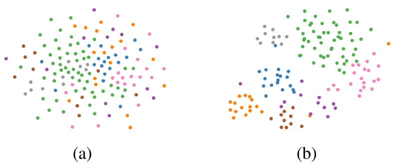
Figure 3: T-SNE visualization of the label representations on WOS dataset. Dots with same color are labels with a same father. (a) BERT model. (b) Our approach.

Our approach attempts to incorporating hierarchy into the text representation, which is fed into a linear layer for probabilities as in Equation 16. The weight matrix $W_{C}$ can be viewed as label representations and we plot theirs T-SNE projections under default configuration. Since a label and its father should be classified simultaneously, the representation of a label and its father should be similar. Thus, if the hierarchy is injected into the text representation, labels with the same father should have more similar representation to each other than those with a different father. As illustrated in Figure 3, label representations of BERT are scattered while label representations of our approach are clustered, which demonstrates that our text encoder can learn a hierarchy-aware representation.

Variants of Graphormer	Micro-F1	Macro-F1
Base architecture	87.46	81.52
-w/o name embedding	86.40	80.40
-w/o spatial encoding	86.88	80.42
-w/o edge encoding	87.25	80.54

Table 4: Performance with variants of Graphormer on development set of WOS. We remove name embedding, spatial encoding, and edge encoding respectively. “w/o” stands for “without”.

Generation Strategy	Micro-F1	Macro-F1
Hierarchy-guided	87.46	81.52
Dropout	86.94	79.91
Random masking	87.19	81.16
Adversarial attack	86.67	80.24

Table 5: Impact of different positive example generation techniques on the development set of WOS. Hierarchy-guided is the proposed method. We control the valid tokens in positive samples roughly the same for random methods. We select FGSM as the attack algorithm following Pan et al. (2021).

5.3.2 Effect of Graphormer

As for the components of the Graphormer, we validate the utility of name embedding, spatial encoding, and edge encoding. As in Table 4, all three components contribute to embedding the graph. Edge encoding is the least useful among these three components. Edge encoding is supposed to model the edge features provided by the graph, but the hierarchy of HTC has no such information so that the effect of edge encoding is not fully embodied in this task. Name embedding contributes most among components. Previous work only initialize embedding weights with label name but we treat it as a part of input features. As a result, neglecting name embedding observes the largest drop, which may explain the poor performance on RCV1-V2.

5.3.3 Effect of Positive Example Generation

To further illustrate the effect of our data generation approach, we compare it with a few generation strategies. Dropout Gao et al. (2021) uses no positive sample generation techniques but contrasts on the randomness of the Dropout function using two identical models. Random masking Meng et al. (2021) is similar to our approach except the remained tokens are randomly selected. Adversarial attack Pan et al. (2021) generates positive examples by an attack on gradients.

As in Table 5, a duplication of the model as positive examples is effective but performs poorly. Instead of dropping information at neuron level, random masking drops entire tokens and boosts Macro-F1 by over 1%, indicating the necessity of building hard enough contrastive examples. The adversarial attack can build hard-enough samples by gradient ascending and disturbance in the embedding space. But the disturbance is not regularized by hierarchy or labels so that it is less effective since there is no guarantee that the adversarial examples remain the label. Our approach guided the example construction by both the hierarchy and the labels, which accommodates with HTC most and achieves the best performance.

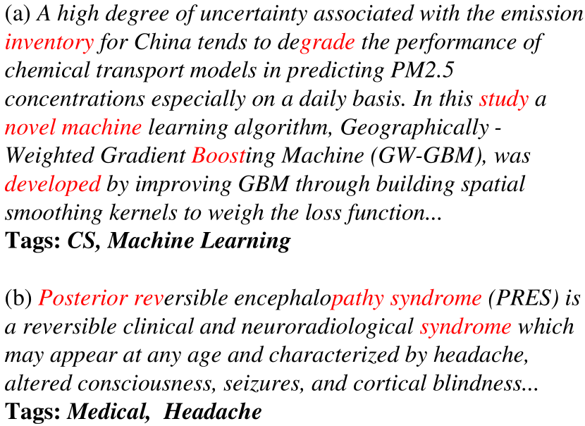
Figure 4: Two fragments of the generated positive examples. Tokens in red are kept for positive examples. We omit a few unrelated tokens (such as a, the, or comma) for clarity.

In Figure 4, we select two cases to further illustrate the effect of labels on positive samples generation. In the first case, word machine strongly indicates this passage belongs to Machine Learning so that it is kept for positive examples. In the second case, syndrome is related to Medical and PRES occurs several times among Headache. Because of the randomness of sampling, our approach cannot construct an example with all keywords. For instance, learning in case one or headache in case two is omitted in this trial, which adds more difficulties for contrastive examples.

6 Conclusion

In this paper, we present Hierarchy-guided Contrastive Learning (HGCLR) for hierarchy text classification. We adopt contrastive learning for migrating taxonomy hierarchy information into BERT encoding. To this end, we construct positive examples for contrastive learning under the guidance of a graph encoder, which learns label features from taxonomy hierarchy. We modify Graphormer, a state-of-the-art graph encoder, for better graph understanding. Comparing to previous approaches, our approach empirically achieves consistent improvements on two distinct datasets and comparable results on another one. All of the components we designed are proven to be effective.

Appendix A Trick for Token Selection

To make sure $P_{i}$ in Equation 10 can acquire gradients, we choose to modify token embedding instead of the token itself. As in Equation 6, $e_{i}$ is the token embedding of $x_{i}$ and can have gradient. The positive counterpart of $e_{i}$ is denoted as:

$$\hat{e_{i}}=e_{i}((P_{i}+Detach(1-P_{i}))\text{ if }P_{i}>\gamma\text{ else }0),$$ (20)

where $Detach$ is a function that ignores the gradient of its input. Numerically, $\hat{e_{i}}$ is either $e_{i}$ or $0$ depending on the threshold $\gamma$, which serves the same purpose as Equation 10. As for gradient,

$$\frac{\partial\hat{e_{i}}}{\partial P_{i}}=e_{i}\text{ if }P_{i}>\gamma\text{ else }0,$$ (21)

which makes $P_{i}$ can be updated by back-propagation.

References

- Alzantot et al. (2018) Moustafa Alzantot, Yash Sharma, Ahmed Elgohary, Bo-Jhang Ho, Mani Srivastava, and Kai-Wei Chang. 2018. Generating natural language adversarial examples. In Proceedings of the 2018 Conference on Empirical Methods in Natural Language Processing, pages 2890–2896, Brussels, Belgium. Association for Computational Linguistics.
- Banerjee et al. (2019) Siddhartha Banerjee, Cem Akkaya, Francisco Perez-Sorrosal, and Kostas Tsioutsiouliklis. 2019. Hierarchical transfer learning for multi-label text classification. In Proceedings of the 57th Annual Meeting of the Association for Computational Linguistics, pages 6295–6300, Florence, Italy. Association for Computational Linguistics.
- Chen et al. (2020a) Boli Chen, Xin Huang, Lin Xiao, Zixin Cai, and Liping Jing. 2020a. Hyperbolic interaction model for hierarchical multi-label classification. In Proceedings of the AAAI Conference on Artificial Intelligence, volume 34, pages 7496–7503.
- Chen et al. (2021) Haibin Chen, Qianli Ma, Zhenxi Lin, and Jiangyue Yan. 2021. Hierarchy-aware label semantics matching network for hierarchical text classification. In Proceedings of the 59th Annual Meeting of the Association for Computational Linguistics and the 11th International Joint Conference on Natural Language Processing (Volume 1: Long Papers), pages 4370–4379, Online. Association for Computational Linguistics.
- Chen et al. (2020b) Ting Chen, Simon Kornblith, Mohammad Norouzi, and Geoffrey Hinton. 2020b. A simple framework for contrastive learning of visual representations. In International conference on machine learning, pages 1597–1607. PMLR.
- Deng et al. (2021) Zhongfen Deng, Hao Peng, Dongxiao He, Jianxin Li, and Philip Yu. 2021. HTCInfoMax: A global model for hierarchical text classification via information maximization. In Proceedings of the 2021 Conference of the North American Chapter of the Association for Computational Linguistics: Human Language Technologies, pages 3259–3265, Online. Association for Computational Linguistics.
- Devlin et al. (2019) Jacob Devlin, Ming-Wei Chang, Kenton Lee, and Kristina Toutanova. 2019. BERT: Pre-training of deep bidirectional transformers for language understanding. In Proceedings of the 2019 Conference of the North American Chapter of the Association for Computational Linguistics: Human Language Technologies, Volume 1 (Long and Short Papers), pages 4171–4186, Minneapolis, Minnesota. Association for Computational Linguistics.
- Fang et al. (2020) Hongchao Fang, Sicheng Wang, Meng Zhou, Jiayuan Ding, and Pengtao Xie. 2020. Cert: Contrastive self-supervised learning for language understanding. arXiv preprint arXiv:2005.12766.
- Gao et al. (2021) Tianyu Gao, Xingcheng Yao, and Danqi Chen. 2021. Simcse: Simple contrastive learning of sentence embeddings. In Proceedings of the 2021 Conference on Empirical Methods in Natural Language Processing, pages 6894–6910.
- Goodfellow et al. (2014) Ian J Goodfellow, Jonathon Shlens, and Christian Szegedy. 2014. Explaining and harnessing adversarial examples. arXiv preprint arXiv:1412.6572.
- Gopal and Yang (2013) Siddharth Gopal and Yiming Yang. 2013. Recursive regularization for large-scale classification with hierarchical and graphical dependencies. In Proceedings of the 19th ACM SIGKDD international conference on Knowledge discovery and data mining, pages 257–265.
- He et al. (2020) Kaiming He, Haoqi Fan, Yuxin Wu, Saining Xie, and Ross Girshick. 2020. Momentum contrast for unsupervised visual representation learning. In Proceedings of the IEEE/CVF Conference on Computer Vision and Pattern Recognition, pages 9729–9738.
- Jang et al. (2016) Eric Jang, Shixiang Gu, and Ben Poole. 2016. Categorical reparameterization with gumbel-softmax. arXiv preprint arXiv:1611.01144.
- Johnson and Zhang (2015) Rie Johnson and Tong Zhang. 2015. Effective use of word order for text categorization with convolutional neural networks. In Proceedings of the 2015 Conference of the North American Chapter of the Association for Computational Linguistics: Human Language Technologies, pages 103–112, Denver, Colorado. Association for Computational Linguistics.
- Kim et al. (2021) Taeuk Kim, Kang Min Yoo, and Sang-goo Lee. 2021. Self-guided contrastive learning for BERT sentence representations. In Proceedings of the 59th Annual Meeting of the Association for Computational Linguistics and the 11th International Joint Conference on Natural Language Processing (Volume 1: Long Papers), pages 2528–2540, Online. Association for Computational Linguistics.
- Kowsari et al. (2017) Kamran Kowsari, Donald E Brown, Mojtaba Heidarysafa, Kiana Jafari Meimandi, Matthew S Gerber, and Laura E Barnes. 2017. Hdltex: Hierarchical deep learning for text classification. In 2017 16th IEEE international conference on machine learning and applications (ICMLA), pages 364–371. IEEE.
- Lai et al. (2015) Siwei Lai, Liheng Xu, Kang Liu, and Jun Zhao. 2015. Recurrent convolutional neural networks for text classification. In Proceedings of the Twenty-Ninth AAAI Conference on Artificial Intelligence, pages 2267–2273.
- Lewis et al. (2004) David D Lewis, Yiming Yang, Tony Russell-Rose, and Fan Li. 2004. Rcv1: A new benchmark collection for text categorization research. Journal of machine learning research, 5(Apr):361–397.
- Mao et al. (2019) Yuning Mao, Jingjing Tian, Jiawei Han, and Xiang Ren. 2019. Hierarchical text classification with reinforced label assignment. In Proceedings of the 2019 Conference on Empirical Methods in Natural Language Processing and the 9th International Joint Conference on Natural Language Processing (EMNLP-IJCNLP), pages 445–455, Hong Kong, China. Association for Computational Linguistics.
- Meng et al. (2021) Yu Meng, Chenyan Xiong, Payal Bajaj, Paul Bennett, Jiawei Han, Xia Song, et al. 2021. Coco-lm: Correcting and contrasting text sequences for language model pretraining. Advances in Neural Information Processing Systems, 34.
- Pan et al. (2021) Lin Pan, Chung-Wei Hang, Avirup Sil, Saloni Potdar, and Mo Yu. 2021. Improved text classification via contrastive adversarial training. arXiv preprint arXiv:2107.10137.
- Peng et al. (2019) Hao Peng, Jianxin Li, Senzhang Wang, Lihong Wang, Qiran Gong, Renyu Yang, Bo Li, Philip Yu, and Lifang He. 2019. Hierarchical taxonomy-aware and attentional graph capsule rcnns for large-scale multi-label text classification. IEEE Transactions on Knowledge and Data Engineering.
- Sandhaus (2008) Evan Sandhaus. 2008. The new york times annotated corpus. Linguistic Data Consortium, Philadelphia, 6(12):e26752.
- Shimura et al. (2018) Kazuya Shimura, Jiyi Li, and Fumiyo Fukumoto. 2018. HFT-CNN: Learning hierarchical category structure for multi-label short text categorization. In Proceedings of the 2018 Conference on Empirical Methods in Natural Language Processing, pages 811–816, Brussels, Belgium. Association for Computational Linguistics.
- Silla and Freitas (2011) Carlos N Silla and Alex A Freitas. 2011. A survey of hierarchical classification across different application domains. Data Mining and Knowledge Discovery, 22(1):31–72.
- Tan et al. (2020) Samson Tan, Shafiq Joty, Min-Yen Kan, and Richard Socher. 2020. It’s morphin’ time! Combating linguistic discrimination with inflectional perturbations. In Proceedings of the 58th Annual Meeting of the Association for Computational Linguistics, pages 2920–2935, Online. Association for Computational Linguistics.
- Vaswani et al. (2017) Ashish Vaswani, Noam Shazeer, Niki Parmar, Jakob Uszkoreit, Llion Jones, Aidan N Gomez, Łukasz Kaiser, and Illia Polosukhin. 2017. Attention is all you need. Advances in neural information processing systems, 30.
- Wang et al. (2021a) Boyan Wang, Xuegang Hu, Peipei Li, and S Yu Philip. 2021a. Cognitive structure learning model for hierarchical multi-label text classification. Knowledge-Based Systems, 218:106876.
- Wang et al. (2021b) Dong Wang, Ning Ding, Piji Li, and Haitao Zheng. 2021b. CLINE: Contrastive learning with semantic negative examples for natural language understanding. In Proceedings of the 59th Annual Meeting of the Association for Computational Linguistics and the 11th International Joint Conference on Natural Language Processing (Volume 1: Long Papers), pages 2332–2342, Online. Association for Computational Linguistics.
- Wehrmann et al. (2018) Jonatas Wehrmann, Ricardo Cerri, and Rodrigo Barros. 2018. Hierarchical multi-label classification networks. In International Conference on Machine Learning, pages 5075–5084. PMLR.
- Wolf et al. (2020) Thomas Wolf, Lysandre Debut, Victor Sanh, Julien Chaumond, Clement Delangue, Anthony Moi, Pierric Cistac, Tim Rault, Remi Louf, Morgan Funtowicz, Joe Davison, Sam Shleifer, Patrick von Platen, Clara Ma, Yacine Jernite, Julien Plu, Canwen Xu, Teven Le Scao, Sylvain Gugger, Mariama Drame, Quentin Lhoest, and Alexander Rush. 2020. Transformers: State-of-the-art natural language processing. In Proceedings of the 2020 Conference on Empirical Methods in Natural Language Processing: System Demonstrations, pages 38–45, Online. Association for Computational Linguistics.
- Wu et al. (2019) Jiawei Wu, Wenhan Xiong, and William Yang Wang. 2019. Learning to learn and predict: A meta-learning approach for multi-label classification. In Proceedings of the 2019 Conference on Empirical Methods in Natural Language Processing and the 9th International Joint Conference on Natural Language Processing (EMNLP-IJCNLP), pages 4354–4364, Hong Kong, China. Association for Computational Linguistics.
- Wu et al. (2020) Zhuofeng Wu, Sinong Wang, Jiatao Gu, Madian Khabsa, Fei Sun, and Hao Ma. 2020. Clear: Contrastive learning for sentence representation. arXiv preprint arXiv:2012.15466.
- Ying et al. (2021) Chengxuan Ying, Tianle Cai, Shengjie Luo, Shuxin Zheng, Guolin Ke, Di He, Yanming Shen, and Tie-Yan Liu. 2021. Do transformers really perform badly for graph representation? Advances in Neural Information Processing Systems, 34.
- Zhang et al. (2020) Wei Emma Zhang, Quan Z Sheng, Ahoud Alhazmi, and Chenliang Li. 2020. Adversarial attacks on deep-learning models in natural language processing: A survey. ACM Transactions on Intelligent Systems and Technology (TIST), 11(3):1–41.
- Zhang et al. (2021) Xinyi Zhang, Jiahao Xu, Charlie Soh, and Lihui Chen. 2021. La-hcn: Label-based attention for hierarchical multi-label text classification neural network. Expert Systems with Applications, page 115922.
- Zhao et al. (2021) Rui Zhao, Xiao Wei, Cong Ding, and Yongqi Chen. 2021. Hierarchical multi-label text classification: Self-adaption semantic awareness network integrating text topic and label level information. In International Conference on Knowledge Science, Engineering and Management, pages 406–418. Springer.
- Zhou et al. (2020) Jie Zhou, Chunping Ma, Dingkun Long, Guangwei Xu, Ning Ding, Haoyu Zhang, Pengjun Xie, and Gongshen Liu. 2020. Hierarchy-aware global model for hierarchical text classification. In Proceedings of the 58th Annual Meeting of the Association for Computational Linguistics, pages 1106–1117, Online. Association for Computational Linguistics.