Connecting Low- and High-Redshift Weak Emission-Line Quasars via HST Spectroscopy of Ly$\alpha$ Emission

Abstract

We present ultraviolet spectroscopy covering the Ly$\alpha$ + N V complex of six candidate low-redshift ($0.9<z<1.5$) weak emission-line quasars (WLQs) based on observations with the Hubble Space Telescope. The original systematic searches for these puzzling Type 1 quasars with intrinsically weak broad emission lines revealed an $N\approx 100$ WLQ population from optical spectroscopy of high-redshift ($z>3$) quasars, defined by a Ly$\alpha$ + N V rest-frame equivalent width (EW) threshold $<15.4$ Å. Identification of lower-redshift ($z<3$) WLQ candidates, however, has relied primarily on optical spectroscopy of weak broad emission lines at longer rest-frame wavelengths. With these new observations expanding existing optical coverage into the ultraviolet, we explore unifying the low- and high-$z$ WLQ populations via EW[Ly$\alpha$+N V]. Two objects in the sample unify with high-$z$ WLQs, three others appear consistent with the intermediate portion of the population connecting WLQs and normal quasars, and the final object is consistent with typical quasars. The expanded wavelength coverage improves the number of available line diagnostics for our individual targets, allowing a better understanding of the shapes of their ionizing continua. The ratio of EW[Ly$\alpha$+N V] to EW[Mg II] in our sample is generally small but varied, favoring a soft ionizing continuum scenario for WLQs, and we find a lack of correlation between EW[Ly$\alpha$+N V] and the X-ray properties of our targets, consistent with a “slim-disk” shielding gas model. We also find indications that weak absorption may be a more significant contaminant in low-$z$ WLQ populations than previously thought.

1 Introduction

Supermassive black holes (SMBHs; $10^{7}\lesssim M_{\rm BH}\lesssim 10^{9}~{}M_{\odot}$) reside in the nuclei of all large galaxies, and it is likely that every SMBH goes through at least one luminous quasar phase where it accretes at $\gtrsim$10% of its Eddington luminosity ($L_{\rm Edd}$; e.g., Soltan 1982; Richstone et al. 1998; Kormendy & Ho 2013). In the standard unification paradigm (e.g., Antonucci, 1993; Urry & Padovani, 1995), one of the most prominent components of unobscured (i.e., Type 1) quasars is the broad emission line region (BELR), where gas embedded deep within the gravitational potential well of the SMBH reprocesses photons from the accretion disk and X-ray corona into Doppler-broadened line emission (e.g., Rees, 1984; Osterbrock & Mathews, 1986; Peterson, 1993; Bentz et al., 2009). These broad lines are observed with typical FWHM $\gtrsim 10^{3}$ km s^-1 in rest-frame optical and ultraviolet (UV) spectroscopy (e.g., Osterbrock & Shuder, 1982).

Examples of Type 1 quasars with unusually weak or missing broad emission lines have emerged over the last $\sim$25 years (e.g., McDowell et al., 1995; Fan et al., 1999; Anderson et al., 2001; Leighly et al., 2007a). Using the Sloan Digital Sky Survey (SDSS; York et al., 2000), Diamond-Stanic et al. (2009, hereafter DS09) performed the first systematic search for these weak-lined quasars (WLQs), revealing the existence of a population of such objects. DS09 measured the rest-frame equivalent width (EW) of the Ly$\alpha$ $\lambda$1216 + N V $\lambda$1240 complex in $\sim$5000 high-redshift ($z>3$) quasars. Finding that the general population follows a log-normal distribution in EW[Ly$\alpha$+N V] except for a $>3\sigma$-weak tail with an excess of $\sim$100 objects, they defined WLQs as having EW[Ly$\alpha$+N V] $<15.4$ Å. They also identified a similar excess in the $>3\sigma$-weak tail of the distribution of the C IV $\lambda$1549 broad emission line, corresponding to EW[C IV] $<10$ Å. The weak BELR in WLQs is very likely an intrinsic feature, i.e., it is not solely an artifact of orientation-induced obscuration or absorption (e.g., Anderson et al. 2001; DS09), gravitational lensing or microlensing (e.g., Shemmer et al. 2006; DS09), and/or Doppler boosting (e.g., Plotkin et al. 2010a; Lane et al. 2011).

WLQs are usually observed to have optical$-$UV continuum shapes similar to those of typical quasars. However, their broad emission lines of high ionization potential (e.g., C IV) appear to be preferentially weakened compared to lines of low ionization potential (e.g., H$\beta$), which suggests their BELR gas is placed in an unusual ionization state by exposure to an abnormally soft photoionizing continuum (e.g., Dietrich et al. 2002; Plotkin et al. 2015, hereafter P15). At the same time, WLQs are also known to exhibit unusual X-ray properties. A relatively large fraction of WLQs ($\sim$50%) are X-ray weak compared to typical quasars ($\lesssim$6%), and they can extend to more extreme values of X-ray weakness (e.g., Ni et al., 2018; Pu et al., 2020). X-ray normal WLQs generally show steep power-law X-ray spectra with a soft excess, suggesting high accretion rates (e.g., Luo et al., 2015; Marlar et al., 2018). On the other hand, the population of X-ray weak WLQs appears to have hard X-ray spectra on average, indicating likely absorption and/or reflection (e.g., Wu et al., 2012; Luo et al., 2015). Furthermore, while the normal radio-quiet quasar population displays a correlation between X-ray weakness and lower EW[C IV] (Gibson et al., 2008), this correlation does not appear to extend to the WLQ population (Ni et al., 2018, 2022; Timlin et al., 2020).

Several physical interpretations have been proposed to explain the above observational characteristics of WLQs. Presently, the foremost is that of a column of “shielding” gas existing between the X-ray corona and BELR (e.g., Wu et al., 2011, 2012; Luo et al., 2015), likely related to the inner edge of an optically- and geometrically-thick, super-Eddington “slim” accretion disk (e.g., Abramowicz et al., 1988; Czerny, 2019) and its wide-angle outflows (e.g., Murray et al., 1995; Castelló-Mor et al., 2017; Jiang et al., 2019; Giustini & Proga, 2019). This configuration is expected to shield the BELR from X-ray and extreme UV radiation emitted by the corona and innermost regions of the accretion disk, softening the incident ionizing continuum. The varied X-ray properties we observe are then explained as a byproduct of orientation, as the edge of the disk and the outflows will obscure X-ray emission from our line of sight at larger inclination angles (Luo et al. 2015; Ni et al. 2022; see also Fig. 1 of Ni et al. 2018).

Alternative explanations have been suggested for the WLQ phenomenon that we describe below for completeness, but we stress that none can also explain the unusual X-ray properties of WLQs (unless WLQs represent a heterogeneous population of objects, and/or multiple mechanisms contribute to their broad line weakness). Other ways to produce preferentially weaker high-ionization potential emission lines include WLQs being powered by exceptionally massive accreting SMBHs ($M_{\rm BH}>3.6\times 10^{9}M_{\odot}$ for non-spinning black holes), which could produce cooler accretion disks with softer ionizing spectra (Laor & Davis, 2011), or super-Eddington accretion producing weaker X-ray coronae, thereby yielding softer, UV-peaked spectral energy distributions (SEDs) (e.g., Leighly et al., 2007a, b). In other cases, it has been suggested that the BELR is gas deficient (e.g., Shemmer et al., 2010; Hryniewicz et al., 2010).

The large sample of WLQs from DS09 consists exclusively of high redshift ($z>3$) objects. This bias is simply an artifact of the SDSS optical spectral range. Nevertheless, WLQ candidates have also been identified at lower redshifts ($z<3$), but with the caveat that their selection is based on weak broad emission lines at longer wavelengths, such as C IV, C III] $\lambda$1909, and/or Mg II $\lambda$2800 (e.g., Collinge et al., 2005; Hryniewicz et al., 2010; Plotkin et al., 2010a, b; Meusinger & Balafkan, 2014). This redshift-based division of the WLQ population poses two problems. First, the lack of a universal standard for classification hampers our ability to confidently unify the two populations (e.g., Nikołajuk & Walter, 2012; Wu et al., 2012; Luo et al., 2015). Second, given that the BELR is expected to produce broad emission lines across the entire rest-frame optical$-$UV range, failure to capture that full range in individual objects prevents the use of diagnostics critical for discriminating between different models for broad line weakness.

Here, we present a pilot study using the Space Telescope Imaging Spectrograph (STIS; Woodgate et al. 1998) aboard the Hubble Space Telescope (HST) to extend existing SDSS optical coverage of six candidate low-redshift WLQs ($1\lesssim z\lesssim 1.5$) into the UV. Our primary objective is to compare EW[Ly$\alpha$+N V] between low- and high-redshift WLQs and assess whether the two populations can indeed be unified. Expanding the wavelength coverage for these six individual objects also increases the number of available line diagnostics, allowing a better understanding of the shapes of their ionizing continua.

The paper is organized as follows: In Section 2, we describe our HST STIS observations and data reduction. Section 3 covers our spectral analysis, including measurement of the UV continuum shape and emission line strengths. We present our results in Section 4 and discuss them in the contexts of the parent quasar and high-redshift WLQ populations in Section 5. Finally, we summarize our conclusions in Section 6. Throughout, we use the term “quasar” to specifically denote Type 1 quasars. We adopt the following cosmology: $H_{0}=67.4$ km s^-1 Mpc^-1, $\Omega_{\rm M}=0.315$, and $\Omega_{\rm\Lambda}=0.685$ (Planck Collaboration et al., 2020).

2 Hubble Space Telescope Observations

2.1 Sample Selection

Figure 1: (a) SDSS i-band absolute magnitude, $M_{i}$ (at $z=2$; see Richards et al. 2006) vs. redshift, $z$. Blue diamonds represent our initial sample of 43 potential target low-$z$ WLQ candidates, and yellow stars represent the final six targets selected for HST observation (see Section 2.1). For comparison, pink squares show the high-$z$ WLQ catalog of DS09. Grey dots represent the 105,783 objects (via a random sample of 5,000) in the full SDSS DR7 quasar catalog (Schneider et al., 2010). (b) Histograms comparing the relative SDSS $\Delta(u-g)$ (top panel) and $\Delta(g-r)$ (bottom panel) color distributions of GALEX-selected (blue hatched bins) vs. rejected (orange dotted bins) objects from our initial sample of 43 potential targets. We find no statistical difference between the GALEX-selected and rejected distributions (see Section 2.1).

We identified potential HST targets by examining lists of $z<3$, weak-featured quasars that were serendipitously recovered during searches for BL Lac objects in SDSS data releases ($\sim$$10^{2}$ objects; Collinge et al., 2005; Anderson et al., 2007; Plotkin et al., 2010b). These quasars passed optical spectroscopic criteria to be classified as BL Lac objects, i.e., all observed emission lines had EW $<5$ Å, and the 4000 Å break, if present, was smaller than $40\%$ (see Plotkin et al. 2010b for details). However, all objects also had faint radio detections or upper limits that firmly placed them in the radio-quiet regime, based on data from the Faint Images of the Radio Sky at Twenty cm survey (FIRST; Becker et al. 1995) and the NRAO VLA Sky Survey (NVSS; Condon et al. 1998). To exclude targets that might have weakly-beamed continua, we only considered objects with radio loudnesses $R<8$, which represents a $>3\sigma$ departure from the expected radio loudness of normal SDSS BL Lac objects (e.g., Plotkin et al. 2010b). We then restricted ourselves to objects with secure redshifts from weak emission features, which left 43 potential targets. The redshifts and SDSS $i$-band magnitudes of these 43 low-$z$ WLQ candidates are shown relative to both the parent SDSS quasar population and high-$z$ WLQs from DS09 in Figure 1a.

To select targets for UV observations with HST, we correlated these 43 objects to the GALEX UV catalogs (Bianchi et al., 2011, 2017). Using a 3 arcsecond match radius and visually examining the GALEX images for each match, we identified 29 sources with suitable GALEX counterparts. The remaining 14 objects were rejected, comprising six matched objects with a GALEX “artifact” or “extractor” flag, two objects lacking a GALEX detection within the match radius, and six objects with locations not covered by GALEX. To determine whether these cuts bias the sample toward objects with bluer continua in their SDSS spectra, we performed Kolmogorov–Smirnov (K-S) and Anderson-Darling (A-D) tests comparing the distributions of the 29 “GALEX-selected” vs. 14 “rejected” objects in relative SDSS optical $\Delta(u-g)$ and $\Delta(g-r)$ colors. The results of these tests are in good agreement with the null hypothesis: for $\Delta(u-g)$, $p=0.69$ and 0.25 from the K-S and A-D tests, respectively, and for $\Delta(g-r)$, $p=0.04$ (K-S) and 0.05 (A-D); see also Figure 1b.

We next restricted the 29-object GALEX-selected sample to include only objects with $0.9<z<1.5$ and GALEX NUV apparent magnitudes $m_{\rm NUV}<19.1$. These cuts were necessary for economical HST observations, allowing us to obtain sufficient signal-to-noise ($>10$ per resolution element) near the continuum of the Ly$\alpha$ + N V emission complex in only 1$-$2 HST orbits per target. After applying the above cuts, we were left with a sample of six candidate WLQs (see Table 1). All six objects have roughly similar optical$-$UV luminosities ($l$_{2500 Å} $\sim 10^{31}$ erg s^-1 Hz^-1). Furthermore, while we did not utilize X-ray emission as an explicit selection criterion, all of our candidates have been observed by the Chandra X-ray Observatory (Wu et al., 2012; Luo et al., 2015), and they fortuitously span nearly the full range of X-ray to optical flux ratios so far observed for WLQs. Throughout this work, we refer to each object by its SDSS designation truncated to the first four digits. All of our targets but one (SDSS J1447) lack coverage of [O III] or H$\beta$ emission, so for consistency we simply adopt the values from Hewett & Wild (2010) as “systemic” redshifts. We do not attempt to measure redshift from Ly$\alpha$ emission as it is expected to be weak/absent in our targets.

2.2 Observations and Data Reduction

Observations with STIS were completed under HST program GO-13298 (PI Plotkin) in Cycle 21, using the NUV-MAMA detector with the G230L grating ($R\approx 500$, dispersion $\Delta\lambda=1.58$ Å pixel^-1) and $52^{\prime\prime}\times 0.2^{\prime\prime}$ slit. One target (SDSS J1447) required two orbits, while the other five targets were each observed in a single orbit. Two exposures per orbit were taken, dithered along the slit in order to correct for cosmic rays and hot pixels. Table 1 summarizes the targets and observations.

Table 1: Sample Properties and HST STIS Observation Log

Source Name	$z$	$m_{\rm NUV}$	$\log l$2500 Å	$L_{\rm bol}/L_{\rm Edd}$	$\alpha_{\rm ox}$	$\Delta\alpha_{\rm ox}$	Obs. Date	Exp. Time
(SDSS J)		(mag)	(erg s-1 Hz-1)					(s)
(1)	(2)	(3)	(4)	(5)	(6)	(7)	(8)	(9)
081250.80+522530.8	1.153	19.13	30.90	$0.23$	$-$2.03a	$-$0.41	2014 Sep 04	2446
090843.25+285229.8	0.933	19.09	30.55	$0.17$	$-$1.46b	0.11	2014 Feb 26	2250
125219.48+264053.9	1.288	18.76	31.06	$0.11$	$-$2.03a	$-$0.39	2014 Apr 24	2270
144741.76$-$020339.1	1.431	19.11	30.97	$1.33$	$-$1.76b	$-$0.13	2014 Aug 22	3593
153044.08+231013.5	1.406	18.76	31.25	$0.32$	$-$1.45a	0.22	2014 Mar 03	2260
162933.60+253200.6	1.340	18.76	30.71	$0.03$	$-$1.62b	$-$0.03	2014 May 08	2230

Note. — Column (1): object name. Column (2): redshift from Hewett & Wild (2010). Column (3): GALEX NUV apparent magnitude (Bianchi et al., 2011, 2017). Column (4): base-10 logarithm of the 2500 Å specific luminosity, $l$_{2500 Å}$=4\pi D^{2}_{\rm L}f$_{2500 Å}$/(1+z)$, where $f$_{2500 Å} is the flux density at 2500 Å from Shen et al. (2011) and $D_{\rm L}$ is the luminosity distance found using the astropy.cosmology package (Astropy Collaboration et al., 2013, 2018). Column (5): Eddington ratio (Mg II-based estimate) from Shen et al. (2011), except for SDSS J1447 (H$\beta$-based estimate) from P15. Column (6): optical$-$UV to X-ray spectral slope $\alpha_{\rm ox}=$ 0.3838 log$(f_{\rm 2keV}/f$_{2500 Å}) (see Section 4.2). Column (7): X-ray weakness parameter $\Delta\alpha_{\rm ox}=\alpha_{\rm ox}-\alpha_{\rm ox,qso}$, where $\alpha_{\rm ox,qso}$ is the value predicted by the $\alpha_{\rm ox}$$-$$l\textsubscript{2500 {\AA}}$ anticorrelation displayed by broad-line radio-quiet quasars (e.g., Steffen et al. 2006; Just et al. 2007; Timlin et al. 2020). For consistency with prior WLQ studies, we adopt the best-fit relationship given by Just et al. (2007). Column (8): HST observation date. Column (9): total HST observation exposure time.

^a Found using $f_{\rm 2keV}$ from Wu et al. (2012).

^b Found using $f_{\rm 2keV}$ from Luo et al. (2015).

Calibrated spectra (at each dither position) were downloaded from the Mikulski Archive for Space Telescopes, which used the calstis v3.4 reduction pipeline. Further processing was performed using the STSDAS package in PyRAF. We first removed the dither offsets using the task sshift, and then combined each sub-exposure using mscomb to create a single spectrum per object. Finally, one-dimensional spectra were extracted using the task x1d with an 11-pixel aperture, which were then corrected for Galactic extinction using the Schlafly & Finkbeiner (2011) recalibration of the Schlegel et al. (1998) maps and adopting a Cardelli et al. (1989) reddening law. The resulting HST UV spectra are presented in Figure 2.

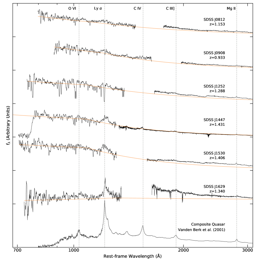
Figure 2: UV spectra redward to 3100 Å for all six target WLQ candidates. The gaps are breaks in spectral coverage; left of the gap is the HST STIS spectrum for all, and right of the gap is the SDSS spectrum for all but SDSS J1447. For SDSS J1447, we instead show the X-shooter spectrum from P15 in order to illustrate its C IV emission. The bottom-most spectrum is the quasar composite from Vanden Berk et al. (2001), shown for comparison. Observed flux density is plotted in solid black, and the fitted power-law continuum (See Section 3.1) is plotted in orange. The vertical axis is the flux density ($f_{\lambda}$) in arbitrary linear units, with ticks denoting the zero-flux level for each spectrum. Our targets have been individually scaled on this axis to display as much detail as possible, while the Vanden Berk et al. (2001) spectrum is scaled to have its $f_{\lambda}$ level at 1450 Å roughly match that of SDSS J0908. The horizontal axis gives the rest-frame wavelength in Å on a log₁₀ scale. Rest-frame wavelength positions of several prominent quasar emission lines are indicated by vertical dashed lines with labels at figure top. The spectra have been smoothed via 1D box convolution (5 pixel width). Note: SDSS J1447 shows a prominent Mg II absorption feature at $\lambda_{\rm rest}\approx 2340$ Å. The apparent strength of this feature is likely enhanced due to noise, as in the observed frame it falls near the UVB/VIS break in X-shooter coverage.

3 Analysis

Table 2: Fitting Parameters and Measurements of Broken Power Law Continua

Source Name	Fit Windowsa	$\lambda_{\rm break}$	$\alpha_{\rm FUV}$	$\alpha_{\rm NUV}$	Comments
(SDSS)		(Å)
(1)	(2)	(3)	(4)	(5)	(6)
J0812	A, D, H, L, O, R, T	$1145.7^{+3.0}_{-195.7}$	$-1.0\pm 0.2$	$-1.4^{+0.3}_{-0.1}$	NAL system at $z\approx 0.79$: Mg II $\lambda 2800$, C IV $\lambda 1549$, Ly$\alpha$, O VI $\lambda 1035$, Ly$\beta$.b
J0908	D, H, L, O, R, T	$1200.0^{+62.4}_{-220.1}$	$-1.0^{+0.4}_{-0.3}$	$-2.0^{+0.3}_{-0.2}$	$\cdots$
J1252	A, D, I, M, O, R, S	$1086.2^{+6.3}_{-35.9}$	$-0.5\pm 0.2$	$-1.5\pm 0.2$	NAL system at $z\approx 1.24$: Si IV $\lambda 1398$, Ly$\alpha$, Ly$\beta$, and O VI $\lambda 1035$.
J1447	C, F, J, K, N, Q	$1084.8^{+8.9}_{-0.6}$	$-0.5\pm 0.1$	$-2.2\pm 0.2$	NAL system at $z\approx 1.03$: Mg II $\lambda 2800$, C IV $\lambda 1549$, Lyman edge.b
J1530	B, G, H, L, P	$1090.5^{+12.9}_{-30.6}$	$-0.3^{+0.2}_{-0.1}$	$-2.0\pm 0.2$	$\cdots$
J1629c	E, H, L, O, R	$\cdots$	$+0.9^{+0.8}_{-1.4}$	$-1.6\pm 0.1$	HST spectrum appears reddened (see Appendix A.6).

Note. — Column (1): object name. Column (2): rest-frame windows used in fitting a broken power law continuum to each object’s full HST STIS spectrum (see Section 3.1). Column (3): wavelength of the power law break. Column (4): best-fit power law index ($f_{\lambda}\propto\lambda^{\alpha_{\lambda}}$) and $1\sigma$ uncertainty for the broken power law fit to the HST FUV continuum (blueward of the break). Column (5): best-fit power law index and $1\sigma$ uncertainty for our broken power law fit to the HST NUV continuum (redward of the break), for all targets but J1629. Column (6): comments on identified NAL systems (see Section 5.3).

^a Continuum fit windows (in Å) corresponding to letter indices in Column (2): A: 800$-$820. B: 810$-$820. C: 811$-$820. D: 850$-$880. E: 855$-$880. F: 850$-$870. G: 870$-$880. H: 1090$-$1105. I: 1085$-$1090. J: 1082$-$1088. K: 1097$-$1102. L: 1140$-$1155. M: 1140$-$1145. N: 1140$-$1149. O: 1280$-$1290. P: 1275$-$1284. Q: 1275$-$1285. R: 1315$-$1325. S: 1350$-$1362. T: 1440$-$1465.

^b Absorption system was tentatively identified by Seyffert et al. (2013).

^c The fit windows listed for SDSS J1629 are used only to find its FUV spectral index ($\alpha_{\rm FUV}$) from the HST spectrum (see Section 3.1). Its NUV spectral index ($\alpha_{\rm NUV}$) is measured from the SDSS continuum, fit using the windows 2150$-$2250 and 3900$-$3940 Å. We do not report a power law break value for this object.

3.1 Continuum

To constrain the continuum shape of each HST UV spectrum, we fit a broken power law model of the form

$$f_{\lambda}\propto\begin{cases}\left(\lambda/\lambda_{\rm break}\right)^{\alpha_{\rm FUV}}&:\lambda<\lambda_{\rm break}\\ \left(\lambda/\lambda_{\rm break}\right)^{\alpha_{\rm NUV}}&:\lambda>\lambda_{\rm break}\end{cases}$$

where $\lambda_{\rm break}$ is the wavelength location of the break. Throughout the rest of this work, we define “FUV” as the portion of the HST spectrum blueward of the break and “NUV” as that redward of the break, so that the spectral indices of the corresponding continua are given by $\alpha_{\rm FUV}$ and $\alpha_{\rm NUV}$, respectively. We perform all spectral analyses in the rest-frame.

The exact range of HST rest-frame spectral coverage varies by target (illustrated in Figure 2), with bounds falling between 675$-$842 Å at the short-$\lambda$ end and 1310$-$1636 Å at the long-$\lambda$ end. There are a number of corresponding rest-frame wavelength windows commonly used for continuum fitting throughout the literature (e.g., Telfer et al., 2002; Diamond-Stanic et al., 2009; Stevans et al., 2014), chosen for their general dearth of emission line contamination. However, most of our six candidates show signatures of narrow absorption line (NAL) systems in their HST spectra, so we customized these windows as needed on a per-object basis. We provide the wavelength ranges adopted for each object in Table 2, along with basic information regarding absorption systems we identified via visual inspection of each spectrum.

We performed the model continuum fit to the observed flux densities (weighted by the $1\sigma$ uncertainty for each measurement) within these spectral windows via a $\chi^{2}$ minimization routine, and we imposed bounds on the break location of $950$ Å $\leq\lambda_{\rm break}\leq 1300$ Å (based on, e.g., Zheng et al., 1997; Telfer et al., 2002; Shang et al., 2005; Stevans et al., 2014). The resulting best-fit spectral indices, $\alpha_{\rm FUV}$ and $\alpha_{\rm NUV}$, are given in Table 2.

To estimate uncertainty in the spectral indices for each object, we used a Monte Carlo algorithm to generate a set of 5,000 mock spectra. We adjusted the flux density of each pixel within our fitting windows via random sampling of a normal distribution where the mean and standard deviation were set respectively to the observed flux density and uncertainty. We then re-fit a broken power law model to each simulated spectrum. We assigned $\pm 1\sigma$ error bars by finding the 16^th and 84^th percentile values of the resulting distributions of $\alpha_{\rm FUV}$ and $\alpha_{\rm NUV}$ from each set of 5,000 simulated spectra.

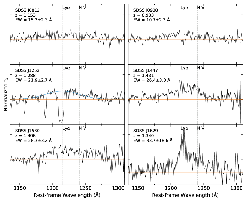
Figure 3: Expanded view of the Ly$\alpha+$N V complex for each WLQ candidate. The orange lines represent the best-fit linear continua. For SDSS J1252, the fitted Gaussian model of the emission complex is shown by a blue curve (see Section 3.2.1). Vertical dashed lines indicate the wavelength locations of Ly$\alpha$ and N V. Note: all objects are shown with identical vertical scale except SDSS J1629, which is shown at a reduced scale to accommodate the full emission feature.

In principle, we could extend the wavelength coverage for our continuum fits by including emission-free regions from the SDSS spectrum of each target. However, there is a risk of flux variability between the SDSS and HST epochs, so we did not utilize the SDSS for our continuum fitting. The only exception is SDSS J1629, which shows a redder spectrum overall and a positive $\alpha_{\rm FUV}$. We attempted to fit a broken power law to only the HST spectrum, but extrapolating the NUV fit to longer wavelengths under-predicted the flux expected from the SDSS at an unreasonable level (see Figure 2), almost certainly because the HST spectrum is more affected by absorption than the SDSS. Thus, for only this source, we fit the NUV continuum using the SDSS spectrum, adopting rest-frame windows 2150$-$2250 and 3900$-$3940 Å. We include the resulting best-fit value as $\alpha_{\rm NUV}$ in Table 2 for completeness, but because SDSS J1629 ultimately does not survive as a WLQ candidate (see Section 4), the exact value adopted for its NUV continuum does not influence any final conclusions.

3.2 Line Measurements

To examine the properties of UV emission lines in our six candidate WLQs, we measured line strength via EW for the Ly$\alpha+$N V complex. We also measured the EW and blueshift of broad C IV emission for SDSS J0908 (the only one of our six targets with this line within the spectral range of our HST observations). The spectral regions covering the Ly$\alpha+$N V and C IV complexes are shown in Figures 3 and 4, respectively.

3.2.1 Ly$\alpha+$N V

We adopted the method described by DS09 (with some slight modifications) to measure the strength of the blended Ly$\alpha+$N V complex. We fit a local linear continuum to each spectrum via a $\chi^{2}$ minimization routine using two 20 Å windows centered on $\lambda$_rest $=$ 1145 Å and 1285 Å (for SDSS J1252, we masked the ranges 1135$-$1138 and 1143$-$1150 Å to avoid significant absorption features). We then performed a simple trapezoidal integration of the normalized flux above the best-fit linear continuum within the range 1160$-$1290 Å to measure the rest-frame EW[Ly$\alpha$+N V]. One candidate, SDSS J1252, shows strong absorption features over the broad Ly$\alpha$ emission (visible in Figure 3 and discussed further in Section 5.3); in this case only, we masked out the wavelengths affected by absorption, fit a single broad Gaussian to model the intrinsic emission profile, and measured EW[Ly$\alpha$+N V] by integrating over the Gaussian model.

Table 3: Emission Line Measurements and Derived Quantities

Source Name	EW[Ly$\alpha$]	EW[C IV]	$\Delta v$[C IV]	EW[Mg II]	$R_{\rm Ly\alpha,MgII}$	$M_{\rm NUV}$
	(Å)	(Å)	(km s-1)	(Å)		(mag)
(1)	(2)	(3)	(4)	(5)	(6)	(7)
SDSS J0812	$15.3\pm 2.3$	$\cdots$	$\cdots$	$8.4\pm 0.7$	$1.83\pm 0.31$	$-25.05\pm 0.29$
SDSS J0908	$10.7\pm 2.3$	$8.3^{+3.8}_{-6.5}$	$1741.9\pm 249.6$	$7.8\pm 1.0$	$1.37\pm 0.34$	$-24.21\pm 0.57$
SDSS J1252	$21.9\pm 2.7$	$\cdots$	$\cdots$	$8.7\pm 0.4$	$2.51\pm 0.33$	$-25.60\pm 0.31$
SDSS J1447a	$26.4\pm 3.0$	$7.7^{+0.2}_{-1.3}$	$1319^{+759}_{-381}$	$13.1^{+2.5}_{-0.1}$	$2.06\pm 0.45$	$-24.89\pm 0.57$
SDSS J1530	$28.3\pm 3.2$	$\cdots$	$\cdots$	$12.9\pm 0.4$	$2.19\pm 0.25$	$-25.34\pm 0.51$
SDSS J1629	$83.7\pm 18.6$	$\cdots$	$\cdots$	$12.3\pm 0.1$	$6.81\pm 1.70$	$-25.62\pm 0.30$
DS09 quasarsb	$63.6^{+38.3}_{-24.0}$	$41.9^{+25.5}_{-15.8}$	$\cdots$	$\cdots$	$\cdots$	$\cdots$
Int-$z$ quasarsc	$\cdots$	$36.6^{+24.9}_{-14.8}$	$\cdots$	$\cdots$	$\cdots$	$\cdots$
Low-$z$ quasarsd	$\cdots$	$\cdots$	$\cdots$	$30.7^{+10.9}_{-8.0}$	$\cdots$	$\cdots$
VB01 compositee	$92.91\pm 0.72$	$23.78\pm 0.10$	$\cdots$	$32.28\pm 0.07$	$2.88\pm 0.02$	$\cdots$

Note. — Column (1): object name. Column (2): measured rest-frame EW and approximate $\pm 1\sigma$ uncertainty for the Ly$\alpha+$N V blend (see Section 3.2.1). Columns (3): measured rest-frame EW and approximate $\pm 1\sigma$ uncertainty for C IV emission (see Section 3.2.2). Column (4): line-of-sight blueshift (defined to be positive for approaching motion) and approximate $\pm 1\sigma$ uncertainty for C IV emission. Column (5): Rest-frame EW and $1\sigma$ uncertainty for Mg II emission, obtained from Shen et al. (2011) except when noted otherwise. Column (6): ratio of Ly$\alpha$ to Mg II line strength, $R_{\rm Ly\alpha,MgII}=$ EW[Ly$\alpha$+N V]$/$EW[Mg II] (see Section 5.2). Column (7): K-corrected NUV absolute magnitude (see Section 4.1).

^aC IV and Mg II measurements for SDSS J1447 are obtained from P15.

^bFor convenience, the final four rows provide quantities from various comparison samples (see Section 3.3 for further description). This row gives the mean values of the log-normal distributions of EW[Ly$\alpha$+N V] and EW[C IV] in the DS09 quasar sample. The quoted uncertainties are the $1\sigma$ ranges of each distribution.

^cThis row gives the mean value of the log-normal distribution of EW[C IV] in the “intermediate-redshift” quasar sample (see Section 3.3). The quoted uncertainty is the $1\sigma$ range of the distribution.

^dThis row gives the mean value of the log-normal distribution of EW[Mg II] in the “low-redshift” quasar sample (see Section 3.3). The quoted uncertainty is the $1\sigma$ range of the distribution.

^eThis row quotes emission line measurements from the Vanden Berk et al. (2001) composite quasar spectrum.

Uncertainties on the best-fit line measurements are dominated by systemic uncertainty in our ability to accurately place the local continuum level. To account for both statistical and systemic uncertainties, we adopted the scheme described in Appendix B.1 of P15. We began with the best-fit local linear continuum and recorded both goodness of fit $\chi^{2}_{\rm best}$ and degrees of freedom $\nu_{\rm best}$. We then generated a $51\times 51$ grid of mock linear continua for each spectrum by varying the observed flux density within each continuum fit window by evenly-stepped factors (ranging between approximately 0.8 and 1.2, depending on the source) across the grid and re-fitting the linear continuum. We compared each $i^{th}$ mock continuum model in the grid to the original spectrum, recording $\chi^{2}_{i}$, computing the relative $\Delta\chi^{2}_{i}=\chi^{2}_{i}-\chi^{2}_{\rm best}$, and measuring EW_i. The $68\%$ ($\sim$1$\sigma$) confidence interval corresponds to continua with $\Delta\chi^{2}_{i}=2.3$ (Avni, 1976). From all continua with $|\Delta\chi^{2}_{i}|$ within this $1\sigma$ confidence range, we recorded the corresponding maximum and minimum EW_i values, and compared these to the best-fit EW measurements to determine approximate $\pm 1\sigma$ uncertainties. EW[Ly$\alpha$+N V] best-fit measurements and uncertainties for all six candidates are given in Table 3.

3.2.2 C IV

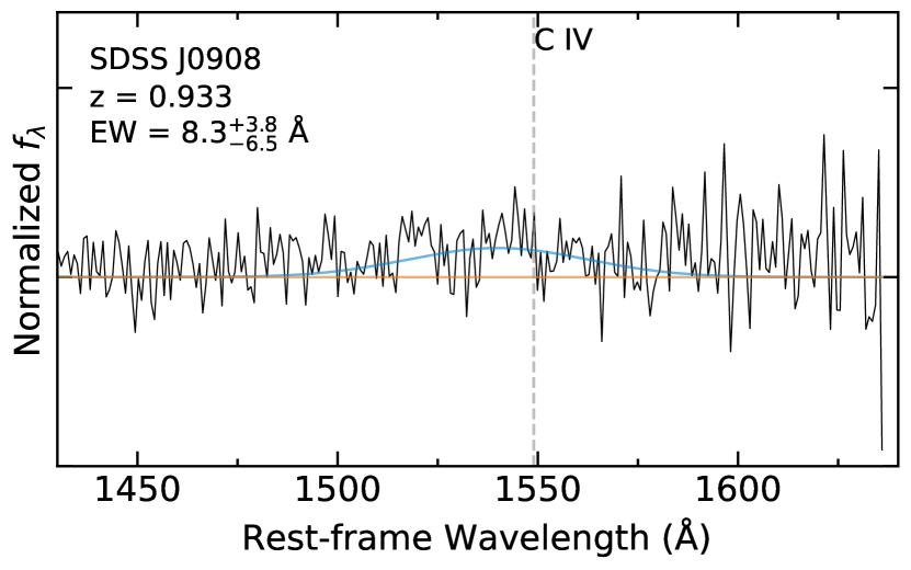
Figure 4: Expanded view of the C IV complex for SDSS J0908. The orange line represents the best-fit linear continuum. The Gaussian model fitted to the emission complex is shown by a blue curve (see Section 3.2.2). The vertical dashed line gives the C IV rest-frame wavelength location to illustrate the blueshift of the observed emission feature.

The HST spectral coverage for SDSS J0908 runs redward to $\lambda$_rest $\approx 1630$ Å, making it unique among our observations in that it provides coverage of C IV emission. For this target, we measured EW[C IV] and its uncertainty in a manner similar to that described in Section 3.2.1, with the local linear continuum fit using windows at $\lambda$_rest $=$ 1435$-$1455 and 1570$-$1580 Å, a single Gaussian curve fit to the emission line feature (shown in Figure 4), and integration performed over the range 1450$-$1580 Å. We also measured the blueshift of the emission line from 1549 Å to the centroid of the Gaussian fit. The results are provided in Table 3.

3.3 Luminosity-Matched Samples of Comparison Radio-Quiet Quasars

To derive a sample of “normal” radio-quiet quasars for comparison of optical$-$UV properties, we considered objects from the SDSS DR7 quasar sample (Schneider et al., 2010) and the Shen et al. (2011) catalog. We limited the selection to quasars targeted for spectroscopy using the algorithm of Richards et al. (2002), and excluded objects identified by Shen et al. (2011) as BAL or radio-loud quasars. We also excluded any objects identified by Collinge et al. (2005) or Plotkin et al. (2010b) as “weak-featured.” To ensure we compare our WLQ candidates to radio-quiet quasars of similar optical$-$UV luminosity and redshift, we limited our selection to the ranges $30.5\leq\log l$_{2500 Å} $\leq 31.5$ (erg s^-1 Hz^-1) and $0.9<z<2.5$. We then found available $m_{\rm NUV}$ measurements by correlating the remaining objects to the GALEX UV catalogs (Bianchi et al., 2017) with a $3^{\prime\prime}$ match radius, excluding any match with a poor quality (i.e., artifact or extractor) flag. There are 14,713 radio-quiet quasars in the resulting set, which we partition further by designating a “low-redshift” quasar sample with $0.9<z<1.5$ (6,381 quasars) and an “intermediate-redshift” quasar sample with $1.5<z<2.5$ (8,332 quasars). Any potentially unidentified WLQs remaining in the sample are likely too few in number to have a significant impact on the statistics.

For easy comparison with average quantities, we add the following information to Table 3 beneath our six targets. We list the mean values of the log-normal distributions of EW[Ly$\alpha$+N V] and EW[C IV] in the high-redshift ($z>3$) quasar sample of DS09, the mean of the log-normal distribution of EW[C IV] in the “intermediate-redshift” quasar sample (using measurements from Shen et al. 2011, limited to 7,906 objects with $>250$ good pixels for C IV), and the mean of the log-normal distribution of EW[Mg II] (again using measurements from Shen et al. 2011, limited to 6,341 objects with $>250$ good pixels for Mg II) in the “low-redshift” quasar sample. We adopt the $1\sigma$ range of each distribution as the quoted uncertainty. In the final row of Table 3, we quote Ly$\alpha$, C IV, and Mg II EW measurements, as well as the ratio $R_{\rm Ly\alpha,MgII}=$ EW[Ly$\alpha$+N V]$/$EW[Mg II] (discussed in Section 5.2), from the Vanden Berk et al. (2001) composite quasar.

4 Results

Figure 5 shows the distribution of EW[Ly$\alpha$+N V] values for our targets in comparison to the DS09 WLQ population. According to the DS09 definition (EW[Ly$\alpha$+N V] $<$ 15.4 Å), only two of our targets qualify as WLQs: SDSS J0812 and SDSS J0908, with EW[Ly$\alpha$+N V] $=15.3\pm 2.3$ and $10.7\pm 2.3$ Å, respectively. SDSS J0908 further qualifies as a WLQ according to its weak EW[C IV] $=8.3^{+3.8}_{-6.5}$ Å (see Section 1).

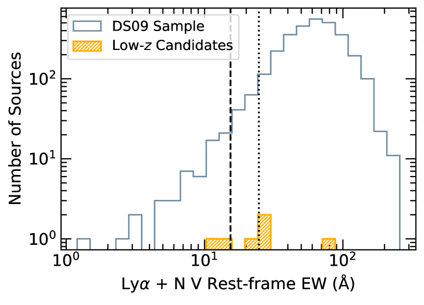
Figure 5: Histogram of the EW[Ly$\alpha$+N V] distribution for our candidate WLQs (orange bins) vs. the full DS09 catalog (blue-outlined bins). Both axes are given on a log scale. The vertical dashed line shows the $3\sigma$ ($<15.4$ Å) weak threshold for WLQ classification, and the vertical dotted line shows the $2\sigma$ ($<27.4$ Å) weak threshold. Two of our targets (SDSS J0812 and SDSS J0908) meet the DS09 criterion for WLQ classification, while one (SDSS J1629) is typical of normal quasars, and the remaining three are somewhat weak ($\sim 2\sigma$) compared to the mean of the best-fit log-normal distribution (see DS09).

Of the remaining four objects, three have EW[Ly$\alpha$+N V] $\approx 20-30$ Å, which is still relatively weak compared to the Vanden Berk et al. (2001) composite quasar spectrum (EW[Ly$\alpha$] $=92.91\pm 0.72$ Å). For reference, the $>2\sigma$-weak tail of the DS09 WLQ distribution corresponds to EW[Ly$\alpha$+N V] $<24.7$ Å. Considering that WLQs represent one extreme of a continuous population, it is therefore likely that these three objects, while not bona fide WLQs, still represent the intermediate part of the population that connects WLQs to normal radio-quiet quasars (as explored for C IV by Ni et al. 2018). This matter introduces an important caveat; while we adopt the same $3\sigma$ and $2\sigma$ weakness thresholds in order to classify our targets in relation to the known population, DS09 (see Section 2 therein) stress that these boundaries are motivated primarily by the statistics of their sample and are therefore somewhat arbitrary. Until a more robust, physically-motivated set of criteria for WLQ selection can be established, the accuracy and precision of such thresholds are uncertain.

The final target, SDSS J1629, has a highly-reddened HST spectrum and shows EW[Ly$\alpha$+N V] $=83.7\pm 18.6$ Å (i.e., typical of normal radio-quiet quasars). This source clearly does not survive as a WLQ candidate, and it is excluded from the remaining discussion (for completeness, its individual properties are discussed in Appendix A.6).

4.1 UV Continuum Properties

Our measured NUV spectral indices ($\alpha_{\rm NUV}$; Table 2) are generally typical of normal quasars (compared to, e.g., $\alpha_{\rm NUV}=-1.54$ from Vanden Berk et al. 2001 and the $\alpha_{\rm NUV}$ distribution shown in Figure 2 of Ivashchenko et al. 2014). Except for SDSS J1629, our measured $\alpha_{\rm FUV}$ values are also generally consistent with normal quasars (e.g., $\alpha_{\rm FUV}=-0.43$ for radio-quiet quasars from Telfer et al. 2002).

Further supporting typical continuum shapes, the observed-frame NUV luminosities of our targets are similar to normal radio-quiet quasars at comparable redshifts and observed-frame optical luminosities. In Table 3 we tabulate $K$-corrected (to $z=0$) absolute NUV magnitudes for our targets, $M_{\rm NUV}=m_{\rm NUV}-DM-K$, where $m_{\rm NUV}$ is the GALEX NUV apparent magnitude (Bianchi et al., 2017), $DM$ is the distance modulus, and $K=2.5\,(1+\alpha_{\rm NUV})\log(1+z)$ is the $K$-correction (see, e.g., Hogg 1999) for which we adopt the best-fit $\alpha_{\rm NUV}$ from each of our candidates. Our targets have a mean absolute magnitude $\langle M_{\rm NUV}\rangle=-25.02\pm 0.47$ (the quoted error is the standard deviation).

We compare our targets’ $M_{\rm NUV}$ values to those of the “low-redshift” quasar sample found in Section 3.3 (calculated as described above, but assuming $\alpha_{\rm NUV}=-1.54$). For this sample, $\langle M_{\rm NUV}\rangle=-24.61\pm 0.65$ (the quoted error is the standard deviation). Given the small number of HST targets, we employ three different non-parametric statistical tests to compare the distributions of $M_{\rm NUV}$, including K-S and A-D tests (both of which compare the distributions of two different populations) and a Mann-Whitney (M-W) test (which compares the means of two populations). No test rejects the null hypothesis, providing $p=0.13$, 0.17, and 0.06 for the K-S, A-D, and M-W tests, respectively. Thus, the UV luminosities of our WLQ candidates appear to be consistent with those of other SDSS-selected radio-quiet quasars at similar redshifts and with similar optical luminosities, with the caveat of small number statistics.

4.2 Comparison of Ly$\alpha$ with X-ray Properties

Figure 6: (a) X-ray to optical flux ratio $\alpha_{\rm ox}$ vs. specific luminosity at 2500 Å. The HST targets are shown by yellow-filled stars, the WLQ sample of Shemmer et al. (2009) by pink-filled squares, and the Ni et al. (2018) extreme and intermediate WLQ samples (including objects from Wu et al. 2012 and Luo et al. 2015) by blue-filled diamonds. Grey dots represent the combined Steffen et al. (2006) and Just et al. (2007) parent quasar samples. Downward arrows represent upper limits on $\alpha_{\rm ox}$ from X-ray non-detections. We adopt $l$_{2500 Å} directly from each reference because the scale shown is not visibly sensitive to minor changes in the adopted cosmology. The dashed line indicates the $\alpha_{\rm ox}$ and $l$_{2500 Å} anticorrelation slope given by Eq. (3) of Just et al. (2007), while the dotted line shows the conventional demarcation between X-ray normal and X-ray weak, $\Delta\alpha_{\rm ox}\leq-0.2$. Our targets have luminosities roughly similar to each other, and they span the range of $\Delta\alpha_{\rm ox}$ for WLQs. (b) $\Delta\alpha_{\rm ox}$ vs. EW[Ly$\alpha$+N V]. Yellow-filled symbols are our HST targets (SDSS designations are given in the legend). The grey-filled squares denote DS09 WLQs for which we have found $\Delta\alpha_{\rm ox}$ using $f_{\rm 2keV}$ measurements from Shemmer et al. (2009) and $f$_{2500 Å} from Shen et al. (2011). The horizontal dotted line indicates the $\Delta\alpha_{\rm ox}\leq-0.2$ demarcation for X-ray weakness, while the vertical dashed line is the EW[Ly$\alpha$+N V] $<15.4$ Å WLQ cutoff. For these samples (both combined and separately), we do not have a correlation between X-ray weakness and Ly$\alpha+$N V emission (see Section 4.2).

To examine our targets in the context of the varied X-ray properties displayed by WLQs (see Section 1), we compare their Ly$\alpha$ and observed X-ray emission strengths. All of our HST targets have been observed by the Chandra X-ray Observatory, and we adopt the $f_{\rm 2keV}$ flux densities tabulated by Wu et al. (2012) and Luo et al. (2015) in addition to the $f$_{2500 Å} flux densities from Shen et al. (2011). Following Tananbaum et al. (1979), we define an object’s optical$-$UV to X-ray spectral slope as

$$\alpha_{\rm ox}=0.3838\log(f_{\rm 2keV}/f\textsubscript{2500 {\AA}}).$$

We also adopt the X-ray weakness parameter,

$$\Delta\alpha_{\rm ox}=\alpha_{\rm ox}-\alpha_{\rm ox,qso},$$

where $\alpha_{\rm ox,qso}$ is the value predicted by the $\alpha_{\rm ox}$ and $l\textsubscript{2500 {\AA}}$ anticorrelation displayed by broad-line quasars (for consistency with prior WLQ studies, we adopt the best-fit relationship given by Eq. (3) of Just et al. 2007; see also, e.g., Steffen et al. 2006; Lusso et al. 2010; Timlin et al. 2020). Our targets’ $\alpha_{\rm ox}$ and $\Delta\alpha_{\rm ox}$ values are given in Table 1, and Figure 6a shows them in relation to the WLQ samples of Shemmer et al. (2009), Wu et al. (2012), Luo et al. (2015), and Ni et al. (2018), as well as quasars from Steffen et al. (2006) and Just et al. (2007).

We compare $\Delta\alpha_{\rm ox}$ against EW[Ly$\alpha$+N V] for our targets combined with the small subset of 6 DS09 WLQs possesssing corresponding $f_{\rm 2keV}$ measurements in the literature (obtained from Shemmer et al. 2009), shown in Figure 6b. Within this sample, there is no correlation between X-ray weakness and Ly$\alpha$ weakness: a Pearson correlation test gives a correlation coefficient $r=0.17$ ($p=0.78$) for our 5-target subset alone, and $r=-0.07$ ($p=0.84$) for the $N=11$ combined sample. This result is consistent with the results of Ni et al. (2018, 2022) and Timlin et al. (2020) for C IV in WLQs.

5 Discussion

We obtained UV spectra of six candidate low-redshift ($0.9<z<1.5$) WLQs using STIS on HST. Our targets were selected primarily on the basis of weak Mg II emission in their SDSS spectra (described in Section 2.1 and tabulated in Table 3), and we have extended their UV coverage blueward to $\sim$700$-$800 Å in the rest-frame. In addition to covering the Ly$\alpha$ + N V complex, this expanded spectral coverage allows more complete constraints on the UV continuum, as well as comparison of the relative strengths of high- and low-ionization emission lines. As noted in Section 4, two of our targets qualify as WLQs based on the weakness of their Ly$\alpha$ + N V emission, and another three may represent the intermediate part of the population (hereafter, simply “intermediate quasars”) between WLQs and typical radio-quiet quasars. We begin this section with a brief discussion of SDSS J0908, which represents our best example of a low-redshift WLQ. More detailed information on each individual target, including SDSS J0908, is provided in Appendix A.

5.1 SDSS J0908, a Low-$z$ WLQ

SDSS J0908 has the weakest Ly$\alpha$ + N V emission among our HST targets, and it also survives as a WLQ on account of its weak broad C IV emission. We quantify the weakness of its C IV emission in the context of the Modified Baldwin Effect (e.g., Baldwin 1977; Baskin & Laor 2004; Shemmer & Lieber 2015), whereby in normal radio-quiet quasars, EW[C IV] is observed to decrease with increasing Eddington ratio ($L_{\rm bol}/L_{\rm Edd}$, a parameterization of the mass-weighted accretion rate). It appears that WLQs tend not to follow this anticorrelation, instead having EW values significantly lower than expected for their $L_{\rm bol}/L_{\rm Edd}$ (Shemmer & Lieber 2015). In SDSS J0908, EW[C IV] is a factor of $\sim$2 weaker than expected (at a significance $>3\sigma$) for its $L_{\rm bol}/L_{\rm Edd}$.

SDSS J0908 also shows moderate blueshift of the broad C IV emission line ($\Delta v$[C IV] $=1741.9\pm 249.6$ km s^-1 relative to the systemic redshift). We interpret this blueshift in the context of “disk-wind” models (e.g., Emmering et al., 1992; Murray et al., 1995; Marziani et al., 1996; Elvis, 2000; Leighly & Moore, 2004; Richards et al., 2011), in which high-ionization BELR emission is dominated at one end of observed EW$-$blueshift parameter space by a disk (or failed wind) component with high EW and low blueshift, and at the other end by a wind component with low EW and high blueshift, likely driven by increasing $L_{\rm bol}/L_{\rm Edd}$ (Giustini & Proga, 2019). Most relevant here is that some WLQs occupy a distinctly wind-dominated regime (e.g., Wu et al. 2012; Luo et al. 2015; P15). The combination of moderately weak and blueshifted C IV and only mildly weak Mg II (see Table 3) in SDSS J0908 is consistent with the disk-wind model and the observed trend for WLQs to move into the wind-dominated regime as C IV EW diminishes (for visual comparison, see Figure 8 of P15).

These results present a curious contrast between the properties of SDSS J0908 and another of our targets, SDSS J1447, for which C IV was measured by P15. As noted above, EW[C IV] in SDSS J0908 is more than $3\sigma$ weaker than expected from the Modified Baldwin Effect. On the other hand, SDSS J1447, despite being weak in C IV per the DS09 paradigm, was found by P15 to be only $\sim$1.5$\sigma$ weaker than expected from the Modified Baldwin Effect (although see caveat below regarding $L_{\rm bol}/L_{\rm Edd}$ derived from virial black-hole mass estimates). Accordingly, P15 predicted that SDSS J1447 is not a WLQ. Indeed, we find that it is insufficiently weak in Ly$\alpha$ + N V emission to qualify as a WLQ (although we reiterate that it may be an intermediate quasar), and its ratio of EW[Ly$\alpha$+N V] to EW[C IV] is higher than SDSS J0908. Dietrich et al. (2002) suggested that the (classical, luminosity-based) Baldwin Effect for high-ionization lines in typical radio-quiet quasars depends partly on the ionization energy of the species, and that the anticorrelation slope is steeper for C IV than for Ly$\alpha$. If this suggestion holds true for the Modified Baldwin Effect, we speculate that the ratio EW[Ly$\alpha$+N V]$/$EW[C IV] in normal radio-quiet quasars might increase with $L_{\rm bol}/L_{\rm Edd}$, and weak C IV in very luminous quasars may not always guarantee weak Ly$\alpha$. Therefore, when attempting to classify high-$L_{\rm bol}/L_{\rm Edd}$ WLQs in the absence of Ly$\alpha$ coverage, it may be useful to first verify that EW[C IV] departs significantly from the Modified Baldwin Effect. However, we caution that the above comparison and interpretation may suffer from substantial systematic uncertainties associated with single-epoch virial black-hole mass estimation techniques (e.g., Shen, 2013, and references therein). The P15 estimate for SDSS J1447 is H$\beta$-based, while the Shen et al. (2011) estimates for our remaining targets (including SDSS J0908) are Mg II-based and are likely to be affected by non-virial motions of the broad line gas (e.g., Wu et al. 2011; P15; Yi et al. 2022, submitted).

Rivera et al. (2022, submitted) suggest parameterizing quasars using the “C IV distance,” as it evaluates objects in relation to a best-fit polynomial curve in EW$-$blueshift parameter space (e.g., see Fig. 12 of Rivera et al. 2020) and may provide a better indicator of $L_{\rm bol}/L_{\rm Edd}$ than the Modified Baldwin Effect. Intriguingly, even in “C IV distance” space, some WLQs could still be outliers. For example, SDSS J0908 and J1447 occupy similar positions in EW$-$blueshift parameter space (and thus have similar C IV distances), yet they display different Ly$\alpha$ properties as discussed in the previous paragraph (with the above caveat of black-hole mass estimation methods).

5.2 Comparison of Optical$-$UV and X-ray Properties

The X-ray and multiwavelength properties of our targets were previously examined by Wu et al. (2012) and Luo et al. (2015), and were found to be most consistent with the slim-disk scenario (Section 1). The expanded wavelength coverage afforded by the HST spectra complements these studies by allowing further tests of the shapes of the objects’ ionizing continua. Notably, we have found a lack of correlation between EW[Ly$\alpha$+N V] and X-ray weakness (Section 4.2) that is also consistent with the slim-disk scenario, as it implies the BELR is exposed to an X-ray$-$optical SED different from the one we observe.

We are also now able to consider the ratio $R_{\rm Ly\alpha,MgII}=$ EW[Ly$\alpha$+N V]$/$EW[Mg II] (see Table 3; except where noted, Mg II measurements are taken from Shen et al. 2011). Unfortunately, we are not aware of a sizable sample of quasars in our targets’ redshift range with uniform coverage of both the Ly$\alpha$ and Mg II complexes, so we limit our comparison to the ratio of “typical” EW values from the Vanden Berk et al. (2001) composite quasar spectrum (listed in Table 3), where $R_{\rm Ly\alpha,MgII}=2.88$. All of our targets fall below this ratio, with a mean of $\langle R_{\rm Ly\alpha,MgII}\rangle=2.0\pm 0.4$ (the quoted error is the standard deviation). The lowest value belongs to our best-confirmed WLQ, SDSS J0908, and for objects with larger EW[Mg II], the ratio tends toward the expectation for typical quasars. This result implies that while both species are weaker than normal, they do not diminish equally; Ly$\alpha$ is preferentially weaker than Mg II, which is generally expected from a soft ionizing SED (and disfavors previous suggestions that WLQ BELRs could be gas deficient). This result is also consistent with studies of other high- to low-ionization line ratios, such as C IV to Mg II and H$\beta$ (e.g., Wu et al. 2012; P15), and it highlights limitations of basing searches for low-$z$ WLQs solely on the properties of low-ionization lines.

Given the slim-disk model’s emphasis on super-Eddington accretion, it is intriguing that our bona fide WLQs do not have particularly high $L_{\rm bol}/L_{\rm Edd}$ estimates, while the intermediate quasar SDSS J1447 does (Table 1). However, we reiterate that these estimates may be highly uncertain, as noted in Section 5.1. Marlar et al. (2018) included SDSS J1447 in a study investigating the X-ray spectra of a sample of WLQs; they found that it had a soft X-ray excess with a steep 0.5$-$8 keV power-law photon index ($\Gamma=2.21^{+0.16}_{-0.15}$) and suggested this result was connected to high $L_{\rm bol}/L_{\rm Edd}$ (based on, e.g., Done et al. 2012). SDSS J0908 was examined in X-ray prior to this by Luo et al. (2015) and, notably, was also found to have a soft X-ray excess with a steep photon index, albeit with a somewhat larger uncertainty ($\Gamma=2.2^{+0.5}_{-0.4}$). It is plausible that $L_{\rm bol}/L_{\rm Edd}$ is simply underestimated for SDSS J0908.

For completeness, we briefly evaluate our targets in the contexts of alternative scenarios for soft ionizing SEDs. Our spectral-index measurements from HST seem to disfavor the exceptionally massive SMBH scenario (Laor & Davis, 2011). We measure $\alpha_{\rm NUV}$ and $\alpha_{\rm FUV}$ typical of normal radio-quiet quasars (see Section 4.1), while Laor & Davis (2011) predict steeply-falling spectra at $\lambda<1000$ Å. There is also the possibility that intrinsic X-ray weakness from a cold accretion disk is responsible for a soft ionizing SED, as with the weak-lined PHL 1811 (Leighly et al., 2007a, b). This interpretation is unlikely to apply to WLQs, however, because: (1) on average, X-ray weak WLQs show signs of X-ray absorption or obscuration (e.g., Wu et al., 2012; Luo et al., 2015); (2) $\sim$50% of the WLQ population is still X-ray normal (e.g., Luo et al., 2015; Ni et al., 2018; Pu et al., 2020); and (3) there does not appear to be a correlation between X-ray weakness and emission-line weakness in the WLQ/intermediate populations (Section 4.2). Indeed, our most securely-confirmed WLQ, SDSS J0908, is X-ray normal ($\Delta\alpha_{\rm ox}=0.11$) and is therefore contrary to the intrinsic X-ray weakness scenario.

5.3 Intrinsic NALs and BALs in Weak-Lined Quasars

There is mounting evidence suggesting that outflow components such as disk winds are generally responsible for intrinsic NAL and BAL features in quasars (e.g., Culliton et al., 2019; Yi et al., 2019a; Lu & Lin, 2019; Rankine et al., 2020), and that some observed properties of wind-dominated quasars, such as C IV emission line blueshift, may arise from the same outflow systems (Yi et al., 2020). Recently, Yi et al. (2019b) observed a Mg II BAL (i.e., “LoBAL,” displaying both low- and high-ionization absorption lines) WLQ with prominent BALs that disappeared and emerged over a period of $\sim$6 years. They suggested this activity was the result of transverse motion of outflowing gas, likely associated with a disk wind. There may be an overlap between wind-dominated WLQs and intrinsic NAL/BAL quasars that has yet to be explored in detail, as most WLQ studies exclude objects with clear signs of BALs to ensure that weak emission features are intrinsic and X-ray results are more straightforwardly interpretable.

Of our targets, SDSS J0812 and SDSS J1447 display signatures of intervening NAL systems, tentatively identified in the SDSS quasar Mg II absorber catalog of Seyffert et al. (2013), and now confirmed via identification of additional, shorter-$\lambda$ absorption lines in the HST spectra (see Table 2). These systems are offset blueward from the objects’ systemic redshifts by $v_{\rm off}>100,000$ km s^-1, such that it is unlikely they are either intrinsic (i.e., physically related to outflows from the central engine) or associated (i.e., observed at the quasar systemic redshift) (e.g., Misawa et al., 2007; Shen & Ménard, 2012).

We have also tentatively identified in SDSS J1252 a narrow absorption system, with a blueward offset $v_{\rm off}\approx 14,400$ km s^-1, that has not been previously reported. Notably, this system lacks an identifiable Mg II $\lambda 2800$ absorption doublet in the SDSS spectrum. The remaining two objects, SDSS J0908 and SDSS J1530, appear to contain narrow absorption features in their HST spectra, and while we cannot identify specific systems, they also do not show corresponding narrow absorption in their SDSS spectra. While this result may be $-$ at least in part $-$ an effect of the SDSS spectral resolution, we cannot discount the possibility that these absorption systems are variable. Intervening NALs are not seen to vary greatly over decade scales, but variability and moderately high velocity offsets are two of the hallmarks expected of intrinsic NALs originating from quasar outflows such as disk winds (e.g., Culliton et al., 2019, and references therein).

While more detailed characterization of these systems is beyond the scope of this paper, an additional feature in the spectrum of SDSS J1252 bears further comment. From the identified NAL system, we expect to see a Mg II $\lambda 1240$ absorption doublet centered on $\lambda$_rest $\approx 1212.5$ Å. Indeed, a strong absorption feature is identified here (see Figure 3). However, this Mg II transition is expected to be relatively weak based on its oscillator strength ($f\lesssim 0.0006$; Kelleher & Podobedova 2008; Danforth et al. 2016, and references therein), and we suspect that the observed feature is instead Ly$\alpha$ from a different, associated absorption system (at $v_{\rm off}\approx 750$ km s^-1 as measured from 1216 Å to the center of the trough). Based on visual examination of the observed trough width, we estimate ${\rm FWHM}\approx 1970$ km s^-1 and tentatively propose that SDSS J1252 is a mini-BAL quasar.

The above results and interpretations imply there may be physical qualities of BAL, mini-BAL, and/or intrinsic NAL quasars that relate to WLQs, but they also hint at weaker, possibly variable, intrinsic absorption systems being a more significant UV-band contaminant in $z<3$ WLQs or intermediate quasars than indicated by SDSS-based surveys of the general quasar population. For example, LoBAL quasars have a tendency to possess redder continua, stronger Fe II emission, and comparatively weak C III] emission in tandem with typical X-ray weakness; this behavior is commonly attributed to a larger viewing angle into the central engine (e.g., Weymann et al., 1991; Voit et al., 1993). Qualitatively, some X-ray weak WLQs and intermediate quasars (such as SDSS J1252) also display these features in contrast to their X-ray normal counterparts (Wu et al., 2012; Luo et al., 2015). If WLQs arise through the slim-disk scenario (in which X-ray weakness and our likelihood of looking “through” winds are both expected to increase with inclination angle), and if WLQ winds are physically similar to those driving BALs and/or intrinsic NALs (e.g., if they are both linked to higher $L_{\rm bol}/L_{\rm Edd}$), then intrinsic absorption at moderate velocity offsets might be more observationally common in X-ray weak WLQs than X-ray normal WLQs (see Rivera et al. 2020 and Richards et al. 2021 for similar discussions in regard to associated absorption lines at the systemic redshift).

Several aspects of WLQ central engines need further exploration before confidently connecting WLQ winds with those driving BALs or intrinsic NALs. For example, the extent to which X-ray variability is possible across the full WLQ population needs characterization (Ni et al., 2020), as does the likelihood of the BAL condition itself contributing to observed X-ray weakness (e.g., Green et al., 1995; Gallagher et al., 2002). This question would benefit from multi-epoch X-ray and optical$-$UV observations (in particular, higher-resolution UV spectra) of verified low-$z$ WLQs, with an emphasis on searching for variable, associated BALs/NALs in a wind-dominated, X-ray weak sample (e.g., Yi et al., 2019b).

6 Summary and Conclusions

We have presented HST STIS UV spectroscopy covering the Ly$\alpha$ + N V complex for six candidate WLQs at low redshift ($0.9<z<1.5$). Combined with the objects’ SDSS spectra, these observations allow direct comparison of high- and low-ionization emission species in individual objects. The HST targets possess UV continuum slopes and luminosities typical of normal radio-quiet quasars. While all six quasars display relatively weak Mg II emission in their SDSS spectra, the new constraints on their Ly$\alpha$ + N V emission qualify only two (SDSS J0812 and SDSS J0908) as bona fide WLQs under the definition introduced by DS09. Additionally, we obtain a constraint on weak C IV emission for SDSS J0908 that further secures its classification as a WLQ. One target (SDSS J1629) appears heavily reddened in its HST spectrum but otherwise shows Ly$\alpha$ + N V emission similar to normal radio-quiet quasars, so it is excluded from analysis. The remaining three targets (SDSS J1252, SDSS J1447, and SDSS J1530) still have somewhat weak Ly$\alpha$ + N V emission and likely represent the intermediate part of the population between WLQs and typical radio-quiet quasars (see Ni et al. 2018). All HST targets were initially selected on the basis of weak Mg II emission, but the observed range of Ly$\alpha$ EW further supports previous conclusions that weak low-ionization lines do not guarantee exceptionally weak high-ionization lines (e.g., Shemmer et al. 2010; Wu et al. 2012; P15; Luo et al. 2015).

The WLQ SDSS J0908 is more than $3\sigma$ weaker in C IV than expected from the Modified Baldwin Effect (e.g., Shemmer & Lieber 2015), while P15 found that SDSS J1447 is only $\sim$1.5$\sigma$ weaker than expected and predicted (correctly) that it does not meet the weak EW[Ly$\alpha$+N V] threshold. We tentatively (with caveats discussed in Section 5.1) suggest that, in the absence of Ly$\alpha$ coverage, it may be useful to verify that a quasar’s EW[C IV] is significantly weaker than predicted by the Modified Baldwin Effect before classifying it as a WLQ. This proposal requires additional validation, however, which may be possible by obtaining a sample of low-$z$ WLQ candidates with coverage of both Ly$\alpha$ and C IV as well as a reliable constraint on $L_{\rm bol}/L_{\rm Edd}$ from multiple estimate techniques (e.g., virial black-hole mass, $\Gamma-L_{\rm bol}/L_{\rm Edd}$ relationship, and/or C IV distance$-L_{\rm bol}/L_{\rm Edd}$ relationship).

We have compared the strengths of high- vs. low-ionization emission lines in our targets via the ratio $R_{\rm Ly\alpha,MgII}=$ EW[Ly$\alpha$+N V]$/$EW[Mg II] and evaluated them in the contexts of various proposed models for BELR weakness. Our targets display a range of comparatively small $R_{\rm Ly\alpha,MgII}$ with preferentially weak Ly$\alpha$, which favors a soft ionizing SED scenario. Furthermore, the UV and X-ray properties of our targets (including a lack of correlation found between EW[Ly$\alpha$+N V] and X-ray weakness) suggest they are not intrinsically X-ray weak, and they appear to be most consistent with the “slim-disk” shielding gas scenario (e.g., Wu et al., 2011, 2012; Luo et al., 2015; Ni et al., 2018, 2022). However, we still cannot dismiss the possibility that WLQs represent a heterogeneous population with multiple mechanisms contributing toward BELR weakness (e.g., P15). Additionally, an open issue remains in that the slim-disk model emphasizes high $L_{\rm bol}/L_{\rm Edd}$, while existing Mg II-based estimates for our bona fide WLQs are not particularly high. The X-ray properties of SDSS J0908 suggest that $L_{\rm bol}/L_{\rm Edd}$ may be underestimated, but this remains to be verified.

Finally, we unexpectedly found evidence of NAL systems in several of the HST spectra, despite little to no sign of their presence in the corresponding SDSS spectra. While the majority of these appear to be intervening systems, we find tentative indications that a NAL system observed in SDSS J1252 may be intrinsic (i.e., physically related to outflows from the central engine). We have also observed a stronger absorption feature overlapping the Ly$\alpha$ emission of SDSS J1252, so we suspect this object may be a mini-BAL quasar. These findings hint at relatively weak absorption being more of a contaminant in the candidate WLQ population than previously thought, posing a challenge to low-$z$ WLQ identification. Given that recent observations of both BALs and associated NALs in normal quasars and WLQs have suggested a wind-driven source or component of absorption (e.g., Culliton et al., 2019; Lu & Lin, 2019; Yi et al., 2019b, 2020), we speculate that in the context of the orientation-dependent, slim-disk shielding gas scenario, intrinsic (though possibly variable) BALs and/or NALs may be more common in X-ray weak WLQs than X-ray normal WLQs. This result provides not only more avenues for comparison between WLQ and normal radio-quiet quasar populations, but also further potential insight into general quasar properties.

Appendix A Notes on Individual Objects

A.1 SDSS J0812

With EW[Ly$\alpha$+N V] $=15.3\pm 2.3$ Å, this object qualifies as a WLQ according to the DS09 criterion. While the 1$\sigma$ uncertainty could plausibly push it above the 15.4 Å threshold, we reiterate that this boundary should not be considered fixed (Section 4; see also Section 2 of DS09). A spectrum covering C IV (which unfortunately falls within the gap between the SDSS and our HST spectra) would be useful to help confirm its WLQ classification.

While we confirm the presence of an intervening NAL system for this object at $z=0.79$ (originally identified in the Mg II absorber catalog of Seyffert et al. 2013), there is no indication this system influences the observed flux within the Ly$\alpha$ measurement range, nor is there any evidence of broad absorption troughs in either the HST or SDSS spectra. We conclude that this object is likely intrinsically weak-lined.

A.2 SDSS J0908

We classify this object as a WLQ, with EW[Ly$\alpha$+N V] $=10.7\pm 2.3$ Å and EW[C IV] $=8.3^{+3.8}_{-6.5}$ Å. Its C IV emission is more than $3\sigma$ weaker than anticipated from the Modified Baldwin Effect (based on its $L_{\rm bol}/L_{\rm Edd}$; e.g., Shemmer & Lieber 2015; with the caveat of virial black-hole mass estimates discussed in Section 5.1), and is also blueshifted ($\Delta v$[C IV] $=1742\pm 249.6$ km s^-1). While this WLQ is X-ray normal ($\Delta\alpha_{\rm ox}=0.11$), its $\Delta\alpha_{\rm ox}-$EW[C IV] relationship is within the observed range for WLQs (e.g., Ni et al., 2018, 2022; Timlin et al., 2020).

While there are possible NAL features in the HST spectrum at short wavelength, no system is identified, and the Ly$\alpha$ measurement range does not appear to be affected. Since there is also no evidence of broad absorption troughs, this object is likely intrinsically weak-lined.

A.3 SDSS J1252

Despite not showing any significant absorption features in its SDSS spectrum, this quasar displays a NAL system at $z=1.24$ in its HST spectrum, as well as a strong, possibly associated Ly$\alpha$ absorber (see Section 5.3). Consequently, we suspect this may be a mini-BAL quasar, although further analysis in this regard is outside the scope of this work. Our EW measurement (EW[Ly$\alpha$+N V] $=21.9\pm 2.7$ Å) may constitute a lower limit, but it nevertheless clearly excludes SDSS J1252 from classification as a WLQ.

A.4 SDSS J1447

SDSS J1447 was studied extensively in the rest-frame optical$-$UV range by P15 using spectra from the X-shooter spectrograph (Vernet et al., 2011) on the Very Large Telescope, producing line measurements for key emission features including H$\alpha$, H$\beta$, Mg II, and C IV. Our HST observation extends rest-frame UV spectral coverage of this quasar blueward from $\sim$1450 Å to $\sim$675 Å, allowing comparison with Ly$\alpha$. Despite SDSS J1447’s mildly weak C IV emission, the strength of its Ly$\alpha$ emission (EW[Ly$\alpha$+N V] $=26.4\pm 3.0$ Å) excludes it from classification as a WLQ. This confirms the conclusion reached by P15, who noted that because its C IV emission was only $\sim$1.5$\sigma$ weaker than expected for its $L_{\rm bol}/L_{\rm Edd}$ and displayed relatively low blueshift, it was likely not a WLQ (instead suggesting it may be an intermediate quasar).

We have confirmed the presence of an intervening NAL system (originally identified by Seyffert et al. 2013) at $z=1.03$ for this quasar. This system includes a Lyman edge visible near the blue limit of the HST spectrum. The broad Ly$\alpha$ emission line may experience some absorption (evidenced by what appears to be a prominent N V $\lambda 1243$ Å remnant; Figure 3), although for the present we do not attempt to characterize this feature.

A.5 SDSS J1530

This object is excluded from WLQ qualification based on the measurement of EW[Ly$\alpha$+N V] $=28.3\pm 3.2$ Å. It displays no detectable NAL features in its SDSS spectrum, and although there may be possible NALs in its HST spectrum, we are unable to identify a system.

A.6 SDSS J1629

This object displays a combined (HST+SDSS) spectrum that is redder than typical, and we have measured a positive-valued FUV continuum slope (i.e., $\alpha_{\rm FUV}>0$). It is not possible to find a broken power law fit that aptly represents the entire observed NUV range, so we measure the NUV continuum slope ($\alpha_{\rm NUV}$) for this quasar using the SDSS spectrum. Its measurement of EW[Ly$\alpha$+N V] $=83.7\pm 18.6$ Å is essentially normal (compared to, e.g., the “typical” $92.91\pm 0.72$ Å from the composite of Vanden Berk et al. 2001), clearly excluding it from classification as a WLQ, and its $L_{\rm bol}/L_{\rm Edd}$ estimate (with the caveat of virial black-hole mass estimates; see Section 5.1) is an order of magnitude smaller than in our other targets. Based on these characteristics, we have largely excluded this quasar from Sections 4 and 5.

Luo et al. (2015) demonstrated that this quasar is neither X-ray weak ($\Delta\alpha_{\rm ox}=-0.02$) nor particularly red in its SDSS spectrum (relative color $\Delta(g-i)=0.01$), yet it appears to have a significantly harder X-ray hardness ratio than most of the WLQ candidates they observed (see their Table 1). Given the appearance of its HST spectrum and the lack of a soft X-ray excess, we suspect it is simply highly absorbed across the UV to soft X-ray band. It is also intriguing that the observed HST flux does not agree well with the GALEX NUV apparent magnitude (see Luo et al. 2015, panel 3 of the extended online version of their Fig. 11, for a visual of the SED incorporating GALEX $m_{\rm NUV}$), further indicating that absorption (or perhaps variability) may be involved. In the optical$-$UV range, it appears the onset of the absorption unfortunately falls within the gap between the HST and SDSS spectra. Combined with this quasar’s somewhat weak Mg II emission, the above results leave the exact state of its ionizing continuum and its physical differences with WLQs and intermediate quasars in question. These questions may yet be useful as drives for future observations of larger samples.

References

- Abramowicz et al. (1988) Abramowicz, M. A., Czerny, B., Lasota, J. P., & Szuszkiewicz, E. 1988, ApJ, 332, 646, doi: 10.1086/166683
- Anderson et al. (2001) Anderson, S. F., Fan, X., Richards, G. T., et al. 2001, AJ, 122, 503, doi: 10.1086/321168
- Anderson et al. (2007) Anderson, S. F., Margon, B., Voges, W., et al. 2007, AJ, 133, 313, doi: 10.1086/509765
- Antonucci (1993) Antonucci, R. 1993, ARA&A, 31, 473, doi: 10.1146/annurev.aa.31.090193.002353
- Astropy Collaboration et al. (2013) Astropy Collaboration, Robitaille, T. P., Tollerud, E. J., et al. 2013, A&A, 558, A33, doi: 10.1051/0004-6361/201322068
- Astropy Collaboration et al. (2018) Astropy Collaboration, Price-Whelan, A. M., Sipőcz, B. M., et al. 2018, AJ, 156, 123, doi: 10.3847/1538-3881/aabc4f
- Avni (1976) Avni, Y. 1976, ApJ, 210, 642, doi: 10.1086/154870
- Baldwin (1977) Baldwin, J. A. 1977, MNRAS, 178, 67P, doi: 10.1093/mnras/178.1.67P
- Baskin & Laor (2004) Baskin, A., & Laor, A. 2004, MNRAS, 350, L31, doi: 10.1111/j.1365-2966.2004.07833.x
- Becker et al. (1995) Becker, R. H., White, R. L., & Helfand, D. J. 1995, ApJ, 450, 559, doi: 10.1086/176166
- Bentz et al. (2009) Bentz, M. C., Walsh, J. L., Barth, A. J., et al. 2009, ApJ, 705, 199, doi: 10.1088/0004-637X/705/1/199
- Bianchi et al. (2011) Bianchi, L., Herald, J., Efremova, B., et al. 2011, Ap&SS, 335, 161, doi: 10.1007/s10509-010-0581-x
- Bianchi et al. (2017) Bianchi, L., Shiao, B., & Thilker, D. 2017, ApJS, 230, 24, doi: 10.3847/1538-4365/aa7053
- Cardelli et al. (1989) Cardelli, J. A., Clayton, G. C., & Mathis, J. S. 1989, ApJ, 345, 245, doi: 10.1086/167900
- Castelló-Mor et al. (2017) Castelló-Mor, N., Kaspi, S., Netzer, H., et al. 2017, MNRAS, 467, 1209, doi: 10.1093/mnras/stx153
- Collinge et al. (2005) Collinge, M. J., Strauss, M. A., Hall, P. B., et al. 2005, AJ, 129, 2542, doi: 10.1086/430216
- Condon et al. (1998) Condon, J. J., Cotton, W. D., Greisen, E. W., et al. 1998, AJ, 115, 1693, doi: 10.1086/300337
- Culliton et al. (2019) Culliton, C., Charlton, J., Eracleous, M., Ganguly, R., & Misawa, T. 2019, MNRAS, 488, 4690, doi: 10.1093/mnras/stz1642
- Czerny (2019) Czerny, B. 2019, Universe, 5, 131, doi: 10.3390/universe5050131
- Danforth et al. (2016) Danforth, C. W., Keeney, B. A., Tilton, E. M., et al. 2016, ApJ, 817, 111, doi: 10.3847/0004-637X/817/2/111
- Diamond-Stanic et al. (2009) Diamond-Stanic, A. M., Fan, X., Brandt, W. N., et al. 2009, ApJ, 699, 782, doi: 10.1088/0004-637X/699/1/782
- Dietrich et al. (2002) Dietrich, M., Hamann, F., Shields, J. C., et al. 2002, ApJ, 581, 912, doi: 10.1086/344410
- Done et al. (2012) Done, C., Davis, S. W., Jin, C., Blaes, O., & Ward, M. 2012, MNRAS, 420, 1848, doi: 10.1111/j.1365-2966.2011.19779.x
- Elvis (2000) Elvis, M. 2000, ApJ, 545, 63, doi: 10.1086/317778
- Emmering et al. (1992) Emmering, R. T., Blandford, R. D., & Shlosman, I. 1992, ApJ, 385, 460, doi: 10.1086/170955
- Fan et al. (1999) Fan, X., Strauss, M. A., Gunn, J. E., et al. 1999, ApJ, 526, L57, doi: 10.1086/312382
- Gallagher et al. (2002) Gallagher, S. C., Brandt, W. N., Chartas, G., & Garmire, G. P. 2002, ApJ, 567, 37, doi: 10.1086/338485
- Gibson et al. (2009) Gibson, R. R., Brandt, W. N., Gallagher, S. C., & Schneider, D. P. 2009, ApJ, 696, 924, doi: 10.1088/0004-637X/696/1/924
- Gibson et al. (2008) Gibson, R. R., Brandt, W. N., & Schneider, D. P. 2008, ApJ, 685, 773, doi: 10.1086/590403
- Giustini & Proga (2019) Giustini, M., & Proga, D. 2019, A&A, 630, A94, doi: 10.1051/0004-6361/201833810
- Green et al. (1995) Green, P. J., Schartel, N., Anderson, S. F., et al. 1995, ApJ, 450, 51, doi: 10.1086/176118
- Hamann & Sabra (2004) Hamann, F., & Sabra, B. 2004, in Astronomical Society of the Pacific Conference Series, Vol. 311, AGN Physics with the Sloan Digital Sky Survey, ed. G. T. Richards & P. B. Hall, 203. https://arxiv.org/abs/astro-ph/0310668
- Harris et al. (2020) Harris, C. R., Millman, K. J., van der Walt, S. J., et al. 2020, Nature, 585, 357, doi: 10.1038/s41586-020-2649-2
- Hewett & Wild (2010) Hewett, P. C., & Wild, V. 2010, MNRAS, 405, 2302, doi: 10.1111/j.1365-2966.2010.16648.x
- Hogg (1999) Hogg, D. W. 1999, arXiv e-prints, astro. https://arxiv.org/abs/astro-ph/9905116
- Hryniewicz et al. (2010) Hryniewicz, K., Czerny, B., Nikołajuk, M., & Kuraszkiewicz, J. 2010, MNRAS, 404, 2028, doi: 10.1111/j.1365-2966.2010.16418.x
- Ivashchenko et al. (2014) Ivashchenko, G., Sergijenko, O., & Torbaniuk, O. 2014, MNRAS, 437, 3343, doi: 10.1093/mnras/stt2137
- Jiang et al. (2019) Jiang, Y.-F., Stone, J. M., & Davis, S. W. 2019, ApJ, 880, 67, doi: 10.3847/1538-4357/ab29ff
- Just et al. (2007) Just, D. W., Brandt, W. N., Shemmer, O., et al. 2007, ApJ, 665, 1004, doi: 10.1086/519990
- Kelleher & Podobedova (2008) Kelleher, D. E., & Podobedova, L. I. 2008, Journal of Physical and Chemical Reference Data, 37, 267, doi: 10.1063/1.2735328
- Kellermann et al. (1989) Kellermann, K. I., Sramek, R., Schmidt, M., Shaffer, D. B., & Green, R. 1989, AJ, 98, 1195, doi: 10.1086/115207
- Kormendy & Ho (2013) Kormendy, J., & Ho, L. C. 2013, ARA&A, 51, 511, doi: 10.1146/annurev-astro-082708-101811
- Lane et al. (2011) Lane, R. A., Shemmer, O., Diamond-Stanic, A. M., et al. 2011, ApJ, 743, 163, doi: 10.1088/0004-637X/743/2/163
- Laor & Davis (2011) Laor, A., & Davis, S. W. 2011, MNRAS, 417, 681, doi: 10.1111/j.1365-2966.2011.19310.x
- Leighly et al. (2007a) Leighly, K. M., Halpern, J. P., Jenkins, E. B., & Casebeer, D. 2007a, ApJS, 173, 1, doi: 10.1086/519768
- Leighly et al. (2007b) Leighly, K. M., Halpern, J. P., Jenkins, E. B., et al. 2007b, ApJ, 663, 103, doi: 10.1086/518017
- Leighly & Moore (2004) Leighly, K. M., & Moore, J. R. 2004, ApJ, 611, 107, doi: 10.1086/422088
- Lu & Lin (2019) Lu, W.-J., & Lin, Y.-R. 2019, ApJ, 887, 119, doi: 10.3847/1538-4357/ab517e
- Luo et al. (2015) Luo, B., Brandt, W. N., Hall, P. B., et al. 2015, ApJ, 805, 122, doi: 10.1088/0004-637X/805/2/122
- Lusso et al. (2010) Lusso, E., Comastri, A., Vignali, C., et al. 2010, A&A, 512, A34, doi: 10.1051/0004-6361/200913298
- Marlar et al. (2018) Marlar, A., Shemmer, O., Anderson, S. F., et al. 2018, ApJ, 865, 92, doi: 10.3847/1538-4357/aad812
- Marziani et al. (1996) Marziani, P., Sulentic, J. W., Dultzin-Hacyan, D., Calvani, M., & Moles, M. 1996, ApJS, 104, 37, doi: 10.1086/192291
- McDowell et al. (1995) McDowell, J. C., Canizares, C., Elvis, M., et al. 1995, ApJ, 450, 585, doi: 10.1086/176168
- Meusinger & Balafkan (2014) Meusinger, H., & Balafkan, N. 2014, A&A, 568, A114, doi: 10.1051/0004-6361/201423810
- Misawa et al. (2007) Misawa, T., Charlton, J. C., Eracleous, M., et al. 2007, ApJS, 171, 1, doi: 10.1086/513713
- Murray et al. (1995) Murray, N., Chiang, J., Grossman, S. A., & Voit, G. M. 1995, ApJ, 451, 498, doi: 10.1086/176238
- Ni et al. (2018) Ni, Q., Brandt, W. N., Luo, B., et al. 2018, MNRAS, 480, 5184, doi: 10.1093/mnras/sty1989
- Ni et al. (2020) Ni, Q., Brandt, W. N., Yi, W., et al. 2020, ApJ, 889, L37, doi: 10.3847/2041-8213/ab6d78
- Ni et al. (2022) Ni, Q., Brandt, W. N., Luo, B., et al. 2022, MNRAS, in press, arXiv:2202.05279. https://arxiv.org/abs/2202.05279
- Nikołajuk & Walter (2012) Nikołajuk, M., & Walter, R. 2012, MNRAS, 420, 2518, doi: 10.1111/j.1365-2966.2011.20216.x
- Noterdaeme et al. (2019) Noterdaeme, P., Balashev, S., Krogager, J. K., et al. 2019, A&A, 627, A32, doi: 10.1051/0004-6361/201935371
- Osterbrock & Mathews (1986) Osterbrock, D. E., & Mathews, W. G. 1986, ARA&A, 24, 171, doi: 10.1146/annurev.aa.24.090186.001131
- Osterbrock & Shuder (1982) Osterbrock, D. E., & Shuder, J. M. 1982, ApJS, 49, 149, doi: 10.1086/190793
- Peterson (1993) Peterson, B. M. 1993, PASP, 105, 247, doi: 10.1086/133140
- Planck Collaboration et al. (2020) Planck Collaboration, Aghanim, N., Akrami, Y., et al. 2020, A&A, 641, A6, doi: 10.1051/0004-6361/201833910
- Plotkin et al. (2010a) Plotkin, R. M., Anderson, S. F., Brandt, W. N., et al. 2010a, ApJ, 721, 562, doi: 10.1088/0004-637X/721/1/562
- Plotkin et al. (2010b) —. 2010b, AJ, 139, 390, doi: 10.1088/0004-6256/139/2/390
- Plotkin et al. (2015) Plotkin, R. M., Shemmer, O., Trakhtenbrot, B., et al. 2015, ApJ, 805, 123, doi: 10.1088/0004-637X/805/2/123
- Pu et al. (2020) Pu, X., Luo, B., Brandt, W. N., et al. 2020, ApJ, 900, 141, doi: 10.3847/1538-4357/abacc5
- Rankine et al. (2020) Rankine, A. L., Hewett, P. C., Banerji, M., & Richards, G. T. 2020, MNRAS, 492, 4553, doi: 10.1093/mnras/staa130
- Rees (1984) Rees, M. J. 1984, ARA&A, 22, 471, doi: 10.1146/annurev.aa.22.090184.002351
- Richards et al. (2021) Richards, G. T., Plotkin, R. M., Hewett, P. C., et al. 2021, ApJ, 914, L14, doi: 10.3847/2041-8213/ac0256
- Richards et al. (2001) Richards, G. T., Fan, X., Schneider, D. P., et al. 2001, AJ, 121, 2308, doi: 10.1086/320392
- Richards et al. (2002) Richards, G. T., Fan, X., Newberg, H. J., et al. 2002, AJ, 123, 2945, doi: 10.1086/340187
- Richards et al. (2006) Richards, G. T., Strauss, M. A., Fan, X., et al. 2006, AJ, 131, 2766, doi: 10.1086/503559
- Richards et al. (2011) Richards, G. T., Kruczek, N. E., Gallagher, S. C., et al. 2011, AJ, 141, 167, doi: 10.1088/0004-6256/141/5/167
- Richstone et al. (1998) Richstone, D., Ajhar, E. A., Bender, R., et al. 1998, Nature, 385, A14. https://arxiv.org/abs/astro-ph/9810378
- Rivera et al. (2022) Rivera, A. B., Richards, G. T., Gallagher, S. C., et al. 2022, ApJ, submitted
- Rivera et al. (2020) Rivera, A. B., Richards, G. T., Hewett, P. C., & Rankine, A. L. 2020, ApJ, 899, 96, doi: 10.3847/1538-4357/aba62c
- Schlafly & Finkbeiner (2011) Schlafly, E. F., & Finkbeiner, D. P. 2011, ApJ, 737, 103, doi: 10.1088/0004-637X/737/2/103
- Schlegel et al. (1998) Schlegel, D. J., Finkbeiner, D. P., & Davis, M. 1998, ApJ, 500, 525, doi: 10.1086/305772
- Schneider et al. (2010) Schneider, D. P., Richards, G. T., Hall, P. B., et al. 2010, AJ, 139, 2360, doi: 10.1088/0004-6256/139/6/2360
- Seyffert et al. (2013) Seyffert, E. N., Cooksey, K. L., Simcoe, R. A., et al. 2013, ApJ, 779, 161, doi: 10.1088/0004-637X/779/2/161
- Shang et al. (2005) Shang, Z., Brotherton, M. S., Green, R. F., et al. 2005, ApJ, 619, 41, doi: 10.1086/426134
- Shemmer et al. (2009) Shemmer, O., Brandt, W. N., Anderson, S. F., et al. 2009, ApJ, 696, 580, doi: 10.1088/0004-637X/696/1/580
- Shemmer & Lieber (2015) Shemmer, O., & Lieber, S. 2015, ApJ, 805, 124, doi: 10.1088/0004-637X/805/2/124
- Shemmer et al. (2006) Shemmer, O., Brandt, W. N., Schneider, D. P., et al. 2006, ApJ, 644, 86, doi: 10.1086/503543
- Shemmer et al. (2010) Shemmer, O., Trakhtenbrot, B., Anderson, S. F., et al. 2010, ApJ, 722, L152, doi: 10.1088/2041-8205/722/2/L152
- Shen (2013) Shen, Y. 2013, Bulletin of the Astronomical Society of India, 41, 61. https://arxiv.org/abs/1302.2643
- Shen et al. (2008) Shen, Y., Greene, J. E., Strauss, M. A., Richards, G. T., & Schneider, D. P. 2008, ApJ, 680, 169, doi: 10.1086/587475
- Shen & Ménard (2012) Shen, Y., & Ménard, B. 2012, ApJ, 748, 131, doi: 10.1088/0004-637X/748/2/131
- Shen et al. (2011) Shen, Y., Richards, G. T., Strauss, M. A., et al. 2011, ApJS, 194, 45, doi: 10.1088/0067-0049/194/2/45
- Soltan (1982) Soltan, A. 1982, MNRAS, 200, 115, doi: 10.1093/mnras/200.1.115
- Steffen et al. (2006) Steffen, A. T., Strateva, I., Brandt, W. N., et al. 2006, AJ, 131, 2826, doi: 10.1086/503627
- Stevans et al. (2014) Stevans, M. L., Shull, J. M., Danforth, C. W., & Tilton, E. M. 2014, ApJ, 794, 75, doi: 10.1088/0004-637X/794/1/75
- Stocke et al. (1992) Stocke, J. T., Morris, S. L., Weymann, R. J., & Foltz, C. B. 1992, ApJ, 396, 487, doi: 10.1086/171735
- Tananbaum et al. (1979) Tananbaum, H., Avni, Y., Branduardi, G., et al. 1979, ApJ, 234, L9, doi: 10.1086/183100
- Taylor (2005) Taylor, M. B. 2005, in Astronomical Society of the Pacific Conference Series, Vol. 347, Astronomical Data Analysis Software and Systems XIV, ed. P. Shopbell, M. Britton, & R. Ebert, 29
- Telfer et al. (2002) Telfer, R. C., Zheng, W., Kriss, G. A., & Davidsen, A. F. 2002, ApJ, 565, 773, doi: 10.1086/324689
- Timlin et al. (2020) Timlin, J. D., Brandt, W. N., Ni, Q., et al. 2020, MNRAS, 492, 719, doi: 10.1093/mnras/stz3433
- Urry & Padovani (1995) Urry, C. M., & Padovani, P. 1995, PASP, 107, 803, doi: 10.1086/133630
- Vanden Berk et al. (2001) Vanden Berk, D. E., Richards, G. T., Bauer, A., et al. 2001, AJ, 122, 549, doi: 10.1086/321167
- Vernet et al. (2011) Vernet, J., Dekker, H., D’Odorico, S., et al. 2011, A&A, 536, A105, doi: 10.1051/0004-6361/201117752
- Virtanen et al. (2020) Virtanen, P., Gommers, R., Oliphant, T. E., et al. 2020, Nature Methods, 17, 261, doi: 10.1038/s41592-019-0686-2
- Voit et al. (1993) Voit, G. M., Weymann, R. J., & Korista, K. T. 1993, ApJ, 413, 95, doi: 10.1086/172980
- Weymann et al. (1981) Weymann, R. J., Carswell, R. F., & Smith, M. G. 1981, ARA&A, 19, 41, doi: 10.1146/annurev.aa.19.090181.000353
- Weymann et al. (1991) Weymann, R. J., Morris, S. L., Foltz, C. B., & Hewett, P. C. 1991, ApJ, 373, 23, doi: 10.1086/170020
- Woodgate et al. (1998) Woodgate, B. E., Kimble, R. A., Bowers, C. W., et al. 1998, PASP, 110, 1183, doi: 10.1086/316243
- Wu et al. (2012) Wu, J., Brandt, W. N., Anderson, S. F., et al. 2012, ApJ, 747, 10, doi: 10.1088/0004-637X/747/1/10
- Wu et al. (2011) Wu, J., Brandt, W. N., Hall, P. B., et al. 2011, ApJ, 736, 28, doi: 10.1088/0004-637X/736/1/28
- Yi et al. (2019a) Yi, W., Brandt, W. N., Hall, P. B., et al. 2019a, ApJS, 242, 28, doi: 10.3847/1538-4365/ab1f90
- Yi et al. (2019b) Yi, W., Vivek, M., Brandt, W. N., et al. 2019b, ApJ, 870, L25, doi: 10.3847/2041-8213/aafc1d
- Yi et al. (2020) Yi, W., Zuo, W., Yang, J., et al. 2020, ApJ, 893, 95, doi: 10.3847/1538-4357/ab7eb8
- Yi et al. (2022) Yi, W., Brandt, W. N., Ni, Q., et al. 2022, ApJ, submitted
- York et al. (2000) York, D. G., Adelman, J., Anderson, John E., J., et al. 2000, AJ, 120, 1579, doi: 10.1086/301513
- Zheng et al. (1997) Zheng, W., Kriss, G. A., Telfer, R. C., Grimes, J. P., & Davidsen, A. F. 1997, ApJ, 475, 469, doi: 10.1086/303560