Self-restricting Noise and Exponential Decay in Quantum Dynamics

Abstract

States of open quantum systems usually decay continuously under environmental interactions. Quantum Markov semigroups model such processes in dissipative environments. It is known that a finite-dimensional quantum Markov semigroup with detailed balance induces exponential decay toward a subspace of invariant or fully decayed states. In contrast, we analyze continuous processes that combine coherent and stochastic processes, precluding detailed balance. First, we find counterexamples to analogous decay bounds for these processes and prove conditions under which they fail. Second, we prove that the relationship between the strength of local noise applied to part of a larger system and overall decay of the whole is non-monotonic. Noise can suppress interactions that would spread it. Faster decay of a subsystem may thereby slow overall decay. We observe this interplay numerically and its discrete analog experimentally on IBM Q systems. Our main results explain and generalize the phenomenon theoretically. Finally, we observe that in spite of its absence at early times, exponential decay re-appears for unital, finite-dimensional semigroups at finite time.

A quantum state exposed to its environment usually decays toward a fixed point that is invariant under environmental interactions. This open-system time-evolution is responsible for decoherence, thermal equilibration, noise in quantum transmission, and many other important processes. An important job of quantum information theory is to understand such decay and its exceptions, estimate rates, and invent strategies to improve control.

Existing theory shows exponential decay for processes involving just noise or thermal equilibration. Much of quantum science, however, involves coherent time-evolution driven by a Hamiltonian, such as gates in quantum computation, interactions in many-body physics, etc. The theory of decay induced by such processes has been less clear. We find that sometimes noise suppresses its own spread, yielding a non-monotonic relationship between noise strength and overall decay rate. Exceedingly strong noise applied to a subsystem often slows the decay it induces on other parts of a system, effectively isolating itself. To summarize the title phenomenon of this paper, self-restricting noise, formalized in Theorem III.3: if a quantum system’s coherent, Hamiltonian-driven dynamics change the fixed point subspace of a dissipative subprocess, then there is a regime in which the rate of decay to the overall fixed point subspace scales inversely with that attributed to the dissipative part by itself.

In addition to reporting the unexpected phenomenon of self-restricting noise, our results fill several missing pieces in the theory of decay. We also find counter-examples to universal exponential decay when combining coherent with noisy processes, a less surprising but important feature. Finally, we observe theoretically that exponential decay still appears above arbitrary, finite timescales for common forms of unital noise and derive a formula estimating the drop in relative entropy. We note potential implications for the theory of quantum capacity, error reduction techniques, and expectations about quantum computing with noise.

To summarize main results:

• We show as Theorem III.3 that noise applied to one part of a coherently interacting system suppresses interactions, slowing its own spread and preserving more information than weaker noise. This Theorem also characterizes circumstances under which short-time exponential decay of relative entropy to a fixed point is assured or violated.

• We show as Theorem III.5 that unital, finite-dimensional semigroups nonetheless induce exponential decay with respect to an arbitrary but finite, minimal timescale. We discuss why this result does not contradict Theorem III.3: as the chosen time unit goes to zero, so must the decay rate.

• In Section IV, we demonstrate a discrete-time, experimental analog of self-restricting noise, in which increasingly frequent application of a completely depolarizing channel to one subsystem reduces the decay induced on an interacting subsystem. These results are obtained from IBM Quantum systems.

Though the paper is primarily theoretical, we also use numerical and experimental examples to illustrate the main phenomena.

I.1 Background

In general, dynamics of open systems are given by quantum channels. A quantum channel is (mathematically) a completely positive, trace-preserving map on densities, and it (physically) models a transformation on a quantum system given by unitary dynamics including both the original system and its environment. When that environment is stationary and dissipative, these dynamics take the form of a quantum Markov semigroup, a family of quantum channels $\Phi^{t}$ parameterized by time $t\geq 0$. Just as a Hamiltonian $H$ generates a family of unitaries $U^{t}=\exp(-itH)$, a Lindbladian $\mathcal{L}$. In mathematics, the Lindbladian would conventionally be a Heisenberg picture superoperator with pre-adjoint $\mathcal{L}_{*}$ acting on densities. Since we work with the Schrödinger picture superoperator on densities, we denote this by $\mathcal{L}$ instead of $\mathcal{L}_{*}$. We nonetheless use the mathematical sign convention that $-\mathcal{L}$ is the generator, rather than $+\mathcal{L}$.generates a quantum Markov semigroup $\Phi^{t}=\exp(-t\mathcal{L})$ [1, 2]. The Lindbladian is an open system generalization of the Hamiltonian to non-unitary dynamics. Quantum Markov semigroups can induce non-invertible processes, as information is lost to the environment.

A series of results [3, 4, 5] have shown that all Lindbladians having detailed balance with respect to a GNS inner product [6] obey a complete, modified logarithmic-Sobolev inequality (CMLSI) based on the modified logarithmic Sobolev inequality defined in [7, 8, 9]. For a semigroup $(\Phi^{t}:t\in\mathbb{R}^{+})$ in terms of the quantum relative entropy $D(\cdot\|\cdot)$, $\lambda$-CMLSI states that

$$D(\Phi^{t}(\rho)\|\Phi^{t}\circ\mathcal{E}(\rho))\leq e^{-\lambda t}D(\rho\|\mathcal{E}(\rho))$$ (1)

for all input densities $\rho$, where $\lambda>0$, and $\mathcal{E}$ is a projection to the fixed point subspace of states that do not decay under $\Phi^{t}$. Furthermore, the “completeness” of the inequality refers to its stability under tensor extensions and products: we may extend $\Phi^{t}$ to $\Phi^{t}\otimes\text{Id}$ for an auxiliary system of any size and the CMLSI constant $\lambda$ remains the same. Though the quantum relative entropy has many information-theoretic interpretations, we use it primarily as as distance-like notion. Decay of relative entropy implies loss of information or distinguishability from a fully decohered or equilibrated fixed point state. CMLSI implies that the diamond norm distance $\|\Phi^{t}-\mathcal{E}\|_{\Diamond}$ and trace distance $d_{\text{tr}}$ of $\Phi^{t}(\rho)$ to a fixed point decay exponentially:

$$\|\Phi^{t}-\mathcal{E}\|_{\Diamond}=2\max_{\rho}d_{\text{tr}}(\Phi^{t}(\rho),\mathcal{E}(\rho))\leq 2e^{-\lambda t/2}\sqrt{\ln d}$$

in dimension $d$, where the maximum includes extensions by an untouched auxiliary system. Diamond norm distance is complementary to process fidelity, which quantifies similarity of channels. CMLSI also implies bounds on decoherence times, capacities, a variety of resource measures, mixing times, and even quantum advantage in near-term algorithms [10, 11, 12]. Properties of relative entropy as discussed in Section III.1 have made general CMLSI more tractable than directly obtaining analogous trace distance bounds.

Nonetheless, important questions have remained open. In particular, detailed balance is often broken when a process includes coherent rotations in addition to noise. Should exponential decay still hold? We consider Lindbladian generators of the form

$$\mathcal{L}(\rho)=i[H,\rho]+\mathcal{S}(\rho)\hskip 2.84544pt$$ (2)

on an input state $\rho$, where $\mathcal{S}$ is a dissipative part, and $H$ a Hamiltonian generator of unitary time evolution. When it exists, we may denote $\mathcal{E}_{0}:=\lim_{t\rightarrow\infty}\exp(-t\mathcal{S})$ as the fixed point subspace projection of $\mathcal{S}$. Similarly, when possible, we denote a projection $\mathcal{E}$ and unitary rotation $R_{t}$ such that $\exp(-t\mathcal{L})\rightarrow\Phi^{t}\circ\mathcal{E}=R_{t}\circ\mathcal{E}$ as the analogous notion of a (potentially rotating) non-decay subspace for $\mathcal{L}$. We refer to $H$ as generating coherent dynamics, rotation, or drift, and to $\mathcal{S}$ as generating stochastic dynamics, noise, or decay. We refer to this combined form as a decay+drift Lindbladian. Under sufficiently loose conditions on $\mathcal{S}$, the form of Equation (2) is universal and admits a unique decomposition into Hamiltonian and dissipative part [2, 13].

Based on results for Lindbladians with GNS detailed balance, one might expect exponential decay to hold generally in the absence of error correction. Analogous to CMLSI, we define a notion of rotated CMLSI with a time-varying, decay-invariant subspace. While this notion extends the concept of CMLSI to include coherent subprocesses, we find it does not hold in general. Some systems decay sub-exponentially at short times as demonstrated in Counterexamples III.1 and III.2. Information may hide in a subsystem or basis that is far in some sense from the noise. More broadly, strong noise induces a competition between Zeno-like effects and long-time decay.

II A Conceptual Preview: Simple Numerical Examples

II.1 Simulated Spin Chain with Depolarizing End

Though the main results of this paper are analytical, we set the stage and build intuition by simulating a simple, commonly studied example: a spin chain in one spatial dimension with open boundary conditions.

1

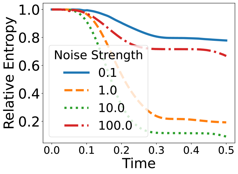
2

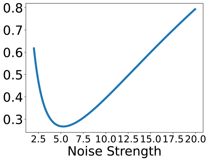
3

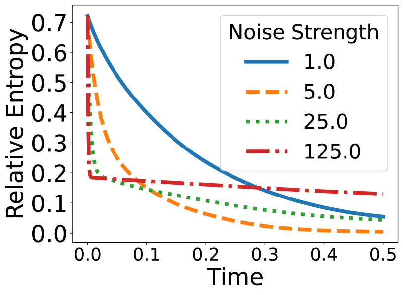
4

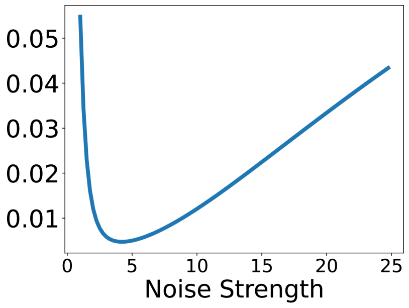
5

Figure 1: Relative entropy of a 4-qubit spin chain to (fully decayed) complete mixture: (1) Spin chain illustration. The noised qubit is on top and shaded yellow. The 3 qubits below are shaded green with nearest-neighbor interactions. (2) Relative entropy vs. time with input $(\hat{1}/2)^{\otimes 3}\otimes|{0}\rangle\langle{0}|$, where the legend notes $\gamma$ in Equation (3); (3) Relative entropy vs. $\gamma$ at time $t=0.5$ with input $\ket{0000}$. (4) Relative entropy vs. time averaged over 50 randomly selected input densities. (5) Relative entropy vs. $\gamma$ averaged over densities at $t=0.5$.

Using Qiskit Dynamics, we simulate $XX+YY$ nearest neighbor interactions (see [14] for a simple example of a similar system) on 4 qubits. We add depolarizing noise to the first qubit in the chain, which continuously randomizes the state of that subsystem concurrently with the aforementioned interactions. The simulated Lindbladian has the form

$$\mathcal{L}=i\Big{[}2\pi\sum_{j=1}^{3}(X_{j}X_{j+1}+Y_{j}Y_{j+1}),\rho\Big{]}-\gamma(\hat{1}/2\otimes\rho^{(2-4)}-\rho)\hskip 2.84544pt,$$ (3)

where $\rho^{(2-4)}$ denotes the marginal on the 2nd-4th qubits, and $X,Y,Z$ denote unnormalized Pauli matrices. We compute relative entropy of the 4-qubit chain with respect to its fixed point of complete mixture, starting from initial state $\ket{0000}$ or $(\hat{1}/2)^{\otimes 3}\otimes|{0}\rangle\langle{0}|$. We also show result for random input densities. Results are plotted in Figure 1. We denote by $\gamma$ a parameter multiplying the noise terms, which controls the strength of noise relative to time and interaction terms. Note that one may technically define the depolarizing channel with depolarizing “probability” greater than 1 - we do not study this regime. Strong noise in our case refers to extremely fast decay to complete mixture, not to extending the parameter range beyond that.

In Figure 1.(2), we examine the model defined by Equation (3) with initial state $(\hat{1}/2)^{\otimes 3}\otimes|{0}\rangle\langle{0}|$. Here we see almost no initial decay, as we examine in Counterexample III.1. More surprising is the inversion in the relationship between noise strength and entropy decay when going from 10.0 to 100.0. Figure 1.(3) further illuminates this observation by showing relative entropy at fixed time as a function of $\gamma$ for input state $\ket{0000}$. To confirm that the effects observed are not state-specific, we also show computations averaged over random density matrix choices. While decay rate expectedly correlates with noise strength for weak noise, the relationship soon inverts. One sees in 1 (2) and (4) a rebound effect, in which stronger noise begins to increase rather than decay the relative entropy at fixed time. The explanation of this phenomenon relies on a Zeno-like effect known as the generalized adiabatic theorem [15]. Extremely strong noise suppresses the interaction between the noised qubit and others, slowing its own spread.

This simple example serves primarily to motivate the the primary studies of this paper. First, however, we turn to an even simpler system.

II.2 An Even Simpler Example

Consider the following scenario: two qubits $A$ and $B$ undergo coherent time-evolution under an interaction Hamiltonian $H=Z\otimes X/2$, while $A$ undergoes depolarizing noise. Hence the system’s evolution is described by the (adjoint) Lindbladian

$$\mathcal{L}(\rho):=i[Z\otimes X/2,\rho]-\gamma(\hat{1}/2\otimes\rho^{B}-\rho)\hskip 2.84544pt.$$ (4)

The fixed point conditional expectation of the stochastic part, $\mathcal{S}(\rho)=-\gamma(\hat{1}/2\otimes\rho^{B}-\rho)$, is $\mathcal{E}_{0}(\rho)=\hat{1}/2\otimes\rho^{B}$. That of $\mathcal{L}$ is $\mathcal{E}(\rho)=\hat{1}/4$, complete mixture. Here $\mathcal{E}_{0}(H)=0$, generating the identity. Let $\Phi_{ZX(t)}$ denote the unitary generated by $H$ in time $t$.

We simulate time-evolution under $\mathcal{L}$ using Qiskit.

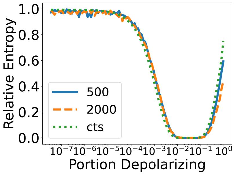
1

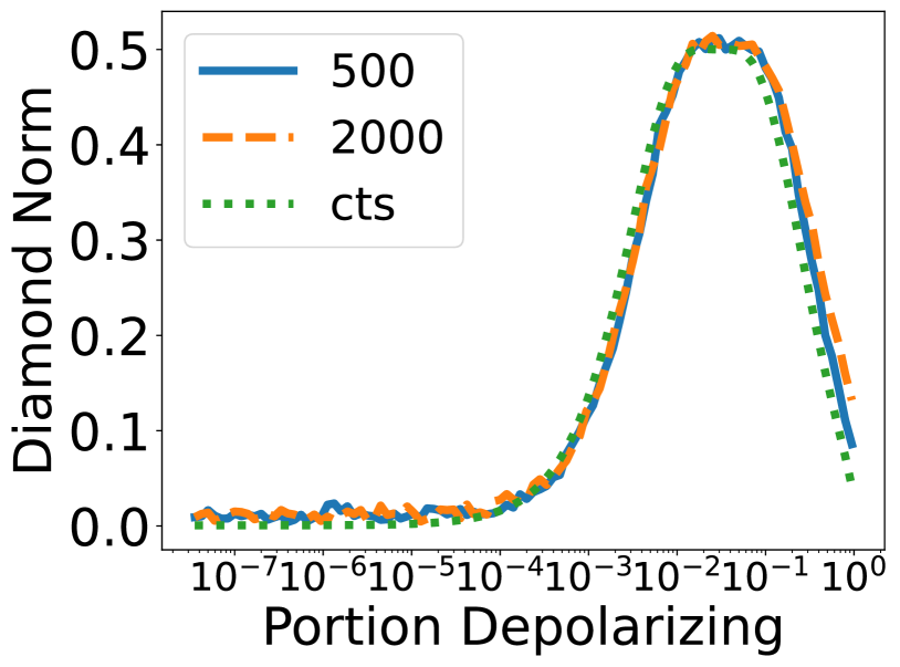
2

Figure 2: Plots of metrics for 2-qubit simulations. Legend shows the number of steps in a Trotter decomposition or “cts” when the simulation is for continuous time in Qiskit Dynamics. (1) Relative entropy of qubit $B$’s state to the fixed point under dephasing, which for this input is completely mixed. (2) Diamond norm distance to the identity (non-decaying) channel.

We first choose $t=4\pi$ so that a fully coherent rotation results in perfect fidelity with the original state. We choose an input state of $|{00}\rangle\langle{00}|$, which decays to complete mixture. We vary $\gamma$ such that $(1-\exp(-\gamma t))$ (the depolarizing likelihood) falls between $3.35*10^{-8}$ and $1.0$, scaled logarithmically. Since qubit $A$ mixes immediately, we study how qubit $B$ decays toward the expected fixed point of complete mixture. Results appear in Figure 2.

We observe counter-intuitively non-monotonic decay with noise strength. For very small values of $\gamma$, the state expectedly does not decay noticeably. As we tune $\gamma$ up, we see a region of strong decay, where a time of $4\pi$ is long enough to mostly dephase qubit $B$ under almost continuous interactions with a regularly noised qubit $A$. With large $\gamma$, however, the relationship inverts. As the noise channel approaches completely depolarizing, we see the decay slow with increasing $\gamma$. We vary Trotter step number to rule this out as an underlying mechanism. Having done so, we proceed to explain the (qualitative) effect theoretically.

III Theoretical Results and Explanation of Observed Phenomena

GNS detailed balance states that for any pair of operators $x,y$, $\text{tr}(\omega x^{\dagger}\mathcal{L}(y))=\text{tr}(\omega\mathcal{L}(x)^{\dagger}y)$, where $\dagger$ denotes Hermitian conjugation. Detailed balance is self-adjointness with respect to the $\omega$-weighted GNS inner product, as described in Subsection III.1 and fully developed in [6]. Often, adding a Hamiltonian term to a Lindbladian breaks GNS detailed balance.

Hamiltonians introduce a technical complication: unitary components in a semigroup may continue to rotate states within protected subspaces indefinitely, so they need not approach a fixed point subspace. Purely Hamltonian time-evolution is the simplest example of a non-trivial semigroup that never decays to a fixed point. To accommodate this and more sophisticated examples, we define (C)MLSI with respect to $\Phi^{t}\circ\mathcal{E}$ as in Equation (1). For semigroups with GNS detailed balance, $\Phi^{t}\circ\mathcal{E}=\mathcal{E}$, so the distinction is ompletely trivial. One may consider our notion to constitute a rotated analog of (C)MLSI if wishing to maintain the $D(\Phi^{t}(\cdot)\|\mathcal{E}(\cdot))$ form exactly.

MLSI does not hold for all finite-dimensional semigroups, as illustrated by the following counterexamples.

Counterexample III.1 (Nearest-Neighbor Interactions with Endpoint Noise).

In this counterexample, we consider an $n$-qubit Hamiltonian of the form $H=\sum_{j=1}^{n}H_{j,j+1}+H_{j}\hskip 2.84544pt.$ This form represents nearest-neighbor interactions on a one-dimensional chain with open boundary conditions. Notable examples include the Heisenberg and Ising models. We also consider a stochastic generator $\mathcal{S}=\mathcal{S}_{1}\otimes\hat{1}^{\otimes n-1}$, which acts only on the leftmost qubit. Physically, we may think of such a system as well-isolated from its noisy environment except for the left end of the chain. Until the $(n-1)$th term in a Taylor expansion of the semigroup around $t=0$, no term contains more than $n-2$ qubit swaps.

Via continuity of relative entropy to a subalgebra restriction (see [16, Lemma 7] and [17, Proposition 3.7]),

$$D(\Phi^{t}(\rho)\|\mathcal{E}(\Phi^{t}(\rho)))\geq(1-O(t^{n-1}\log t))D(\rho\|\mathcal{E}(\rho))\hskip 2.84544pt.$$

Since $\Phi^{t}$ cannot have MLSI with any $\lambda>0$, it does not have MLSI.

To be more specific, consider a swap chain in which $H=\sum_{j=1}^{n-1}X_{j}X_{j+1}+Y_{j}Y_{j+1}$ as in Subsubsection II.1. Let $A_{1},...,A_{n}$ denote qubit subsystems . We add a stochastic generator of noise on the 1st qubit, $\mathcal{S}(\rho)=\rho-\hat{1}/2\otimes\text{tr}_{A_{1}}(\rho)$. The equilibrium state of the swap chain is an overall complete mixture. Now consider the input state $\rho=(\hat{1}/2)^{\otimes(n-1)}\otimes|{0}\rangle\langle{0}|$, which is in equilibrium everywhere except the rightmost qubit. Relative entropy decay at small $t$ proceeds as $O(t^{n-1}\log t)$, representing sublinear tunneling amplitude for the state at one end to undergo noise at the other. The fixed point accounts for propagation of noise throughout the entire system, but noise takes time to propagate along the chain. This counterexample is illustrated numerically in Subsubsection II.1.

Counterexample III.2 (Dephasing + Basis Drift).

Consider the Lindbladian

$$\mathcal{L}(\rho)=i[X,\rho]-\gamma(Z\rho Z-\rho)\hskip 2.84544pt,$$

where $X,Z$ are the usual qubit Pauli matrices. This Lindbladian combines rotation via the Pauli $X$ matrix with dephasing in the $Z$ basis. The long-term behavior of this Lindbladian is depolarizing, as any state not in the $Z$ basis becomes more mixed, and a state diagonal in the $Z$ basis rotates to another basis. We apply $\mathcal{L}$ to the input state $|{0}\rangle\langle{0}|$. Again using continuity of relative entropy to a subalgebra restriction,

$$D(\Phi^{t}(|{0}\rangle\langle{0}|)\|\hat{1}/2)\geq(1-O(t^{2}\log t))D\big{(}|{0}\rangle\langle{0}|\big{\|}\hat{1}/2\big{)}\hskip 2.84544pt.$$ (5)

Analogously to how in Counterexample III.1 noise takes time to propagate between qubits, here it takes time to propagate between bases. This counterexample to MLSI also recalls the quantum Zeno effect [18].

For a Lindbladian in the form of Equation (2), the fixed point of the stochastic generator $\mathcal{S}$ will not coincide with the overall fixed point of the process unless its projector $\mathcal{E}_{0}$ commutes with $H$. When these fixed point projectors differ, a system initially in the fixed point subspace of $\mathcal{S}$ takes time to see decay. Furthermore, strong noise can actually suppress its own spread:

Theorem III.3 (Self-restricting Noise).

Let $\mathcal{L}(\rho)=i[H,\rho]+\mathcal{S}(\rho)$ be a decay+drift Lindbladian generating semigroup $\Phi^{t}$ with fixed point conditional expectation $\mathcal{E}$ up to a possible persistent rotation. Assume that for every input density $\rho$, $\Phi_{0}^{t}(\rho):=\exp(-t\mathcal{S})(\rho)$ decays exponentially in trace distance or relative entropy to $\mathcal{S}$’s fixed point subspace with rate at least $\lambda_{0}$.

• If $H$ commutes with $\Phi_{0}^{\infty}$, and $\lambda_{0}$ is the (C)MLSI constant of $\Phi^{t}_{0}$, then $\mathcal{E}=\Phi_{0}^{\infty}$, and

  $$\hskip 21.68231ptD(\Phi^{t}(\rho)\|\Phi^{t}\mathcal{E}(\rho))\leq e^{-\lambda_{0}t}D(\rho\|\mathcal{E}(\rho))\text{ for all }t>0\hskip 2.84544pt.$$

If $H$ does not commute with $\Phi_{0}^{\infty}$, then…

• …for some input densities $\rho$ and asymptotically small $t$,

  $$\hskip 21.68231ptD(\Phi^{t}(\rho)\|\Phi^{t}\mathcal{E}(\rho))\geq(1-O(t^{2}\log t))D(\rho\|\mathcal{E}(\rho))>0\hskip 2.84544pt.$$

• … if the relative entropy or trace distance of $\Phi^{t}(\rho)$ to a fixed point decays exponentially for every input $\rho$ with rate $\lambda$ at sufficiently long times, then $\lambda\leq O(\|H\|_{\infty}/\sqrt{\lambda_{0}})$.

A formal, technical version of Theorem III.3’s final statement with calculable constants appears as Theorem B.17 in the Supplementary Information, and the proof of the complete Theorem appears thereafter. Furthermore, Theorem B.17 generalizes $H$ to another Lindbladian $\mathcal{L}_{1}$ under some assumptions about fixed point subspace projections. Theorem III.3 assumes the existence of a fixed point projection $\mathcal{E}_{0}$ for $\mathcal{S}$ and overall fixed point projection $\mathcal{E}$ up to rotation, which is necessary for the usual formulation of exponential decay to make sense.

The surprising aspect of Theorem III.3 is not the breakdown of CMLSI at short times, but that the decay rate of $\mathcal{L}$, $\lambda$, is upper-bounded inversely to that of $\mathcal{S},\lambda_{0}$. Theorem III.3 starts to explain the observations in Section II. In the limit of infinite noise strength, the system approaches Zeno dynamics generated by $\mathcal{E}_{0}(H)$ acting on $\mathcal{E}_{0}(\rho)$ - see Theorem III.8. While Zeno dynamics immediately apply the maximal decay induced by $\mathcal{S}$, they also constrain how $H$ can effectively change $\mathcal{E}_{0}$, maintaining protected subspaces from $\mathcal{S}$ that would otherwise be exposed via interplay with $H$. As a common example discussed subsequently, one may consider a Lindbladian of the form $\mathcal{L}(\rho)=i[H,\rho]+\gamma\mathcal{S}(\rho)$ for $\gamma>0$ such that $H$ and $\mathcal{S}$ do not commute. As $\gamma\rightarrow\infty$, the overall decay induced by $\mathcal{L}$ to its fixed point subspace scales as $1/\sqrt{\gamma}$. This effect emerges when the ratio of dissipative strength to Hamiltonian strength is large - it would not necessarily appear, for instance, as one increases an overall scale parameter affecting both $H$ and $\mathcal{S}$.

In general, if a Lindbladian’s Hamiltonian does not commute with the decay part’s invariant projection, overall CMLSI will fail at short times, and self-restriction will appear for strong noise. In practice, one might expect noise to affect different bases or subsystems heterogeneously, but not so much that it only applies to one part. Analogous results apply: weakly noised subsystems’ initial decay reflects their decay rates at short times rather than those of interacting, noisier subsystems.

Example III.4.

Rather than model noise via semigroup dynamics, a common alternative defines an explicit environment coupled to the system via Hamiltonian interaction terms (for instance, see [19, 20]). Intuitively, one might expect to recover dissipative semigroup dynamics on the original system by adding dissipative noise to the environment in such a model, then taking the noise strength to infinity: $\mathcal{L}(\cdot)=i([H_{sys},\cdot]+[H_{int},\cdot])+\gamma\mathcal{S}_{env}(\cdot)$, where $\mathcal{S}_{env}$ applies depolarizing noise as in Section II as $\gamma\rightarrow\infty$. We see, however, that this intuition fails: as $\gamma\rightarrow\infty$, the interaction Hamiltonian $H_{int}$ reduces to Zeno dynamics generated by $\mathcal{E}_{sys}(H_{int})$, acting unitarily on the original system.

Despite the failure of CMLSI and appearance of self-restricting noise, we still expect exponential decay with estimable rate after finite time:

Theorem III.5 (Exponential Decay with Drift).

Let $(\Phi^{t})$ be a unital, finite-dimensional semigroup. For any $\tau>0$, there is some $\lambda_{\tau}<1$ such that

$$D(\Phi^{t}(\rho)\|\Phi^{t}\circ\mathcal{E}(\rho))\leq\lambda_{\tau}^{\lfloor t/\tau\rfloor}D(\rho\|\mathcal{E}(\rho))$$

for all $t>0$, where $\lfloor\cdot\rfloor$ denotes the floor function. The same $\lambda_{\tau}$ holds under extensions of the form $\Phi^{t}\rightarrow\Phi^{t}\otimes\hat{1}^{B}$ on any finite-dimensional auxiliary system $B$.

In Section III.1, we also derive a concrete way of calculating $\lambda_{\tau}$ in the technical version, Theorem III.16. When $\mathcal{L}$ describes purely unitary time-evolution, Theorem III.5 is trivially satisfied with equality - $\mathcal{E}$ becomes the identity, and $D(\Phi^{t}(\rho)\|\Phi^{t}\mathcal{E}(\rho))=0$ for all $\rho$ and $t>0$.

Theorem III.5 is somewhat of a counterpoint to Theorem III.3, showing that CMLSI-like decay appears at intermediate-long timescales, albeit with constants that may depend in a complicated, non-monotonic way on prior noise strength parameters. To understand the assumptions and constants in Theorem III.5 and how they compare with Theorem III.3, we examine how distinct regimes compare qualitatively to observations in Subsection II.2. We consider a Lindbladian of the form $\mathcal{L}(\rho)=i[H,\rho]+\gamma\mathcal{S}(\rho)$, in which the explicit parameter $\gamma>0$ tunes noise strength. As a specific example, we recall Equation (4). Analyzing distinct regimes:

• For small $\gamma$, $\Phi^{t}(\rho)\approx\exp(-it[H,\cdot])(\rho)$. Relative entropy decays slowly. In Figure 2, this regime corresponds roughly to 0-1% depolarizing noise.

• The regime of strongest overall decay appears for intermediate values of $\gamma$, such as with 1-10% depolarizing noise in Figure 2.

• When $\gamma$ is large and $t$ not too small, $\Phi^{t}\approx\tilde{R}_{t}\mathcal{E}_{0}$ for rotation $\tilde{R}_{t}$ generated by $\mathcal{E}_{0}(H)$. This modified Hamiltonian generates Zeno dynamics, which may explore subspaces remaining invariant under $\mathcal{E}_{0}$ and $\mathcal{S}$. This regime corresponds to 10-100% depolarizing noise in Figure 2. Self-restriction as in Theorem III.3 protects information in the fixed point subspace of $\mathcal{S}$, which might be larger than the fixed point subspace of $\mathcal{L}$.

Though Theorem III.5 agrees qualitatively with simulation, we expect the quantitative correspondence to be loose. The simulations of Subsection II use input states chosen to show large effects in low dimension. Theorem III.5 trades away this optimality in magnitude for generality.

Exponential decay is known for quantum circuits undergoing local depolarizing noise, which constrains quantum advantage for optimization problems [11]. In a distinct but related model, heralded dephasing noise was also shown to induce exponential convergence to complete mixture [21]. Though many prior works including [11] and [21] model noise as occurring between gate layers, real circuits combine both gate-simultaneous and passive noise. We see via Theorem III.5 that random gates create depolarizing from dephasing and similar noise:

Corollary III.6.

Consider an ensemble of circuits of fixed depth, where each gate is approximated by a sequence of time-independent Hamiltonians. Let each layer have a probability at least $q\in(0,1)$ to apply each gate in a set that is universal for single qubits. Let each qubit in the system simultaneously undergo noise via a mixture of unitaries. Then the system’s expected relative entropy and trace distance to complete mixture decay exponentially.

This Corollary is proven in Supplementary Information Subsection B.3. In contrast, we consider some implications of Theorem III.3 . Let a Hamiltonian time-evolution or quantum circuit implemented by successive Hamiltonians undergo simultaneous…

• …extremely strong, depolarizing noise on some qubits for the total duration of execution. Then from the output one may approximately recover the output of a smaller, noiseless circuit $\tilde{C}$, which is known post-execution and insulated from the strong noise.

• …uniform, per-qubit, extremely strong dephasing noise for the total duration of execution. Then an input in the invariant basis is approximately unchanged at output, as Zeno dynamics suppress gate executions.

Both statements are consequences of self-restricting noise. The second above scenario may hint at why macroscopic, unshielded systems, which likely experience strong environmental dephasing, can maintain definite, classical states instead of randomizing under out-of-basis Hamiltonians.

Due to their tensor-stability, decay inequalities such as CMLSI can bound quantum capacities [10]. Via the Lloyd-Shor-Devetak Theorem [22, 23, 24], the quantum capacity $Q(\Phi)$ of quantum channel $\Phi$ has an expression given by a regularized quantum relative entropy. Hence the results of Theorem III.3 and Theorem III.5 apply to quantum capacity. In particular, we would see in a process such as described by Equation (4) that the channel has capacity of approximately 2 qubits in the regime of negligible noise, zero quantum capacity in intermediate regimes at sufficiently long times, and capacity of 1 qubit in the strong noise limit. A Shannon-theoretic consequence of self-restricting noise is the re-emergence of non-zero quantum capacity under strong dissipation.

Example III.7.

Consider a simple model of a propagating photon carrying one qubit each in its polarization and orbital angular momentum (OAM) degrees of freedom, such as in [25], but passing through a hypothetical medium that couples polarization to OAM. If the photon undergoes depolarizing noise in the OAM degree of freedom, then the relative entropy to a fully-depolarized state may follow the curves shown in Figure 2. As noise strength increases, the quantum capacity of the channel goes to zero, and it later becomes entanglement-breaking. However, as the noise strength is increased further, it will eventually regain the capability to transmit entanglement, and even regain non-zero capacity.

A related phenomenon to Theorem III.3 is that fast dissipation may protect systems from Hamiltonian interactions with other environment systems [26], acting as a sort of error suppression. While this phenomenon is known for the quantum Zeno effect, our Theorem III.8 implies that such effects may occur via continuous, semigroup-driven dissipation, not just through discrete, interrupting measurements. Furthermore, our results show explicitly how the power of these schemes relates to the protective dissipation having a large CMLSI or trace norm decay constant. While strong, universal lower bounds on decay rates are usually bad news for those seeking to avoid decoherence, fast decay can become protective.

III.1 Mathematical Derivation of the Main Results

By $\mathbb{B}(\mathcal{H})$ we denote the space of bounded operators on Hilbert space $\mathcal{H}$, and by $\mathcal{D}(\mathcal{H})$ we denote the space of densities. By $\hat{1}$ we denote the identity matrix. For a unitary matrix $U$, we denote by $R_{U}$ the channel that applies that unitary matrix via conjugation such that $R_{U}(X):=UXU^{\dagger}$ for any $X\in\mathbb{B}(\mathcal{H})$. If there is a family of unitaries $(U_{j})$, we may denote $R_{j}:=R_{U_{j}}$ when it is clear from context. A quantum channel is a completely positive, trace-preserving map, usually denoted by $\Phi,\Psi,$ or $\Theta$. For products of quantum channels, we use concatenation to denote composition or the “$\circ$” symbol to optimize readability, e.g. $\Phi\Psi(\rho)=\Phi(\Psi(\rho))=\Phi\circ\Psi(\rho)$. We often use the diamond norm to compare quantum channels, denoted $\|\cdot\|_{\Diamond}$. We also characterize similarity of quantum densities using the fidelity given by $F(\rho,\omega)=\text{tr}(\sqrt{\sqrt{\rho}\omega\sqrt{\rho}})^{2}$. By process fidelity we refer to the fidelity between Choi matrices. See Appendix A for more information on norms used in this paper.

Relative entropy inequalities herein are restricted to finite dimension, though they should in principle extend to infinite dimension with re-derivation of some referenced inequalities. The Zeno-like norm bounds derived in Appendix B in principle generalize to some infinite-dimensional settings, but that is not the focus of this paper.

A quantum Markov semigroup (QMS) is a family of channels $(\Phi^{t})$ for $t\in\mathbb{R}^{+}$ (continuous case) or $t\in\mathbb{N}$ (discrete case) with the essential property that $\Phi^{t}\Phi^{s}=\Phi^{t+s}$. For any quantum channel $\Phi$, $(\Phi^{t}:t\in\mathbb{N})$ is a discrete semigroup of powers of the channel. Any continuous QMS has an adjoint Lindbladian generator $\mathcal{L}$ such that $\Phi^{t}=\exp(-t\mathcal{L})$ for any $t\in\mathbb{R}^{+}$. For a Hamiltonian $H$, we denote by $i[H,\cdot]$ the transformation given by $i[H,\cdot](x):=i[H,x]$ for an operator $x$. Hence $R_{\exp(-iHt)}=\exp(-i[H,\cdot])$. A Lindbladian generalizes Hamiltonian time-evolution to open systems.

For a normal, faithful density $\omega\in\mathcal{D}(\mathcal{H})$, the GNS inner-product with respect to $\omega$ is defined for $x,y\in\mathbb{B}(\mathcal{H})$ as $\braket{x,y}_{\omega}=\text{tr}(\omega x^{*}y)$ in a tracial setting. We say that a Lindbladian has GNS detailed balance or that $\mathcal{L}$ is GNS self-adjoint when $\mathcal{L}$ is self-adjoint with respect to the GNS inner product for an implied (or explicitly written) invariant density $\omega$. Formally, the standard Lindbladian is $\mathcal{L}^{*}$, the adjoint of $\mathcal{L}$ with respect to the trace.

Any Lindbladian with GNS detailed balance has a fixed point subspace $\mathcal{N}_{\omega}$ related to its fixed point von Neumann algebra $\mathcal{N}$ [6]. There is a fixed point projector $\mathcal{E}_{\omega}$ to $\mathcal{N}_{\omega}$, the pre-adjoint of a conditional expectation $\mathcal{E}_{\omega}^{*}$ with respect to the trace. As with the Lindbladian, we denote by $\mathcal{E}$ the completely positive, trace-preserving or Schrödinger picture quantum channel, and by $\mathcal{E}^{*}$ its adjoint. We may refer to $\mathcal{E}$ as a conditional expectation. We may denote by $\mathcal{E}$ a conditional expectation or related channel, at times suppressing the explicit subscript. Some additional properties of $\mathcal{E}$ are described in Appendix A. We also recall the Pimsner-Popa indices, which we denote for subspace projections,

$$\begin{split}&C(\mathcal{E})=\inf\{c>0|\rho\leq c\mathcal{E}(\rho)\forall\rho\in\mathcal{M}_{*}\}\\ &C_{cb}(\mathcal{E})=\sup_{n\in\mathbb{N}}C(\mathcal{E}\otimes\text{Id}^{n})\hskip 2.84544pt.\end{split}$$

as considered in [17, 5] and originally by Pimsner and Popa [27] as a finite-dimensional analog of the Jones index [28]. When $\mathcal{E}$ has is GNS self-adjoint with respect to density $\omega$, $C_{cb}(\mathcal{E})\leq d^{2}\omega_{\text{min}}^{-1}$, where $d$ is the dimension of the space and $\omega_{\text{min}}^{-1}$ the minimum eigenvalue of $\omega$.

A starting point for this work is the quantum version of the modified logarithmic Sobolev inequality (MLSI) introduced by Kastoryano and Temme [9]. Stochastic versions of this inequality appear in earlier literature [7, 8]. MLSI differs from but was inspired by the earlier notion of logarithmic Sobolev inequalities [29, 30]. An important, more recent observation is that while the canonical log-Sobolev inequality fails for semigroups that lack a unique fixed point state [31], the modified version may remain valid [32]. This observation motivated the notion of a complete modified logarithmic-Sobolev inequality (CMLSI) [33]. A finite-dimensional semigroup generated by $\mathcal{L}$ has $\lambda$-CMLSI if and only if

$$\begin{split}&D\big{(}\big{(}e^{-\mathcal{L}t}\otimes\hat{1}^{B}\big{)}(\rho)\big{\|}\big{(}e^{-\mathcal{L}t}\otimes\hat{1}^{B}\big{)}\circ(\mathcal{E}\otimes\hat{1}^{B})(\rho)\big{)}\\ &\leq e^{-\lambda t}D(\rho\|(\mathcal{E}\otimes\hat{1})(\rho))\end{split}$$ (6)

for all extensions by a finite-dimensional auxiliary subsystem $B$. In the literature, CMLSI is often stated equivalently with $(\mathcal{E}\otimes\hat{1}^{B})(\rho)$ as the second argument to the left-hand side relative entropy. One might take this as the definition and consider our notion to constitute a “rotated” CMLSI-like notion. CMLSI with some constant is known for all finite-dimensional quantum Markov semigroups having GNS detailed balance with respect to a faithful state. This result was derived in a self-contained way in [5]. It was simultaneously derived in [4] for semigroups that are self-adjoint with respect to the trace, which via [3] also extends to all finite-dimensional semigroups with detailed balance.

Though the quantum Zeno effect is historically stated in terms of measurements [18], a number of results that include versions of the generalized Zeno effect [34, 35, 36, 37, 38], dynamical decoupling [19, 20], and adiabatic theorems [39, 15] show that many kinds of fast quantum processes can modify the effective dynamics of a simultaneous, slower process. Here we show a Zeno-like bound in terms of CMLSI constants:

Theorem III.8.

Let $\mathcal{L}$ be a bounded Lindbladian and $t>0$. Let $\Phi$ be any quantum channel with fixed point subspace projection $\mathcal{E}_{0}$. If $D(\Phi(\rho)\|\mathcal{E}(\rho))\leq e^{-\lambda}D(\rho\|\mathcal{E}(\rho))$ for all $\rho$ including auxiliary extensions or if $\|\Phi^{k}-\mathcal{E}_{0}\|_{\Diamond}\leq e^{-\lambda k}b$ for constant $b>0$ and large $k\in\mathbb{N}$, then

$$\|\big{(}\Phi\circ e^{-\mathcal{L}t/k}\big{)}^{k}-e^{-\mathcal{E}_{0}\mathcal{L}\mathcal{E}_{0}t}\mathcal{E}_{0}\|_{\Diamond}\leq\begin{cases}O(t^{2}/k)\text{ any $\lambda$ }\\ O(t^{2}/\lambda k)\text{ small $\lambda$.}\end{cases}$$

For any Lindbladian $\mathcal{S}$ such that $\|e^{-\mathcal{S}t}-\mathcal{E}_{0}\|_{\Diamond}\leq e^{-\lambda t}b$ (as implied by $\lambda$-CMLSI),

$$\big{\|}e^{-(\mathcal{S}+\mathcal{L})t}-e^{-\mathcal{E}_{0}\mathcal{L}\mathcal{E}_{0}t}\mathcal{E}_{0}\big{\|}_{\Diamond}\leq O\Big{(}\frac{t^{2}}{\lambda}\Big{)}\hskip 2.84544pt.$$

If $\mathcal{L}=i[H,\cdot]$ for some Hamiltonian $H$, then $\exp(-\mathcal{E}_{0}\mathcal{L}\mathcal{E}_{0}t)\circ\mathcal{E}_{0}(\rho)$ is equivalent to unitary evolution generated by $\mathcal{E}_{0}(H)$ applied to $\mathcal{E}_{0}(\rho)$ for any input $\rho$.

Theorem III.8 is a version of the generalized quantum Zeno effect. For continuous dissipation, it is sometimes referred to as an adiabatic theorem or watchdog effect. Theorem III.8 is a shortened version of Theorem B.14, Remark B.16, and Remark B.6, which derives constants, can account for time-varying interruption channels in the discrete case, and may for some cases substitute alternate norm conditions. The semigroup generated by $\mathcal{E}_{0}\mathcal{L}\mathcal{E}_{0}$ is conventionally referred to as the Zeno dynamics. For discrete interruption by a fixed point projection as in Subsection IV, Proposition B.5 yields a more specific bound with tighter constants.

Though Theorem III.8 is similar to results of [15, 36, 38], it bounds convergence in terms of CMLSI and decay constants. This distinction may seem subtle, but it is essential to Theorem III.3, which compares decay constants of a Lindbladian and its rotation-free constituent. Furthermore, the asymptotic dependence on $t$ and $\mathcal{L}$ is explicitly shown and of polynomial order. As seen in Example B.18, there are cases in which stronger decay does not arise from multiplicative comparability. The primary argument of the proof is that the first order terms in Taylor series for the original dynamics and Zeno limit are equivalent after expanding in both the number of discrete steps ($k$ in Theorem III.8) and a matrix order comparison parameter determined by the decay constant. The result then follows from analytically and combinatorially bounding the higher-order terms in both of these parameters. To derive the continuous case, we use a Kato-Suzuki-Trotter formula in the $k\rightarrow\infty$ limit. Because Theorem III.8 is similar to known inequalities, we state it as a method rather than a main result of this paper. Still, it is possible that Theorem III.8 is of independent interest.

Proving Theorem III.5 is subtle because of the possibility for Zeno-like effects to block decay to the long-time fixed point subspace. A method of intuitive relevance noted in [40, 41] allows one to build up MLSI estimates for a complicated system from simpler subprocesses. Were we to follow that philosophy, we might attempt to combine decay estimates from effective noise processes at different times. A counter-intuitive consequence of Theorem III.8 and the broader Zeno effect, however, is that a chain of projections may approach the action of a unitary on a particular subspace. Let $\mathcal{E}_{t}:=R_{\exp(-iHt)}\circ\mathcal{E}_{0}\circ R_{\exp(iHt)}$ for Hamiltonian $H$ and any $t\in\mathbb{R}$. Note that for any $k\in\mathbb{N}$, $\mathcal{E}_{t}\mathcal{E}_{t-1/k}...\mathcal{E}_{1/k}=R_{\exp(-iHt)}\circ(\mathcal{E}_{0}R_{\exp(iHt/k)})^{k}\hskip 2.84544pt$. As a direct consequence,

$$\lim_{k\rightarrow\infty}\mathcal{E}_{t}\mathcal{E}_{t-1/k}...\mathcal{E}_{1/k}\mathcal{E}_{0}=R_{\exp(i(\mathcal{E}_{0}(H)-H)t)}\circ\mathcal{E}_{0}$$ (7)

Though each $\mathcal{E}_{t},...,\mathcal{E}_{1/k}$ is a projection that we might interpret as rotation-free, in the continuum limit, the chain of composed projections approaches unitary rotation following $\mathcal{E}_{0}$. In the limit, such a chain of conditional expectations does not induce decay of a state toward an intersection of fixed point subspaces but rotates the subspace projected to by $\mathcal{E}_{0}$.

Ultimately, however, we obtain Theorem III.5. To prove it, we first recall the notion of the multiplicative domain: for a unital channel $\Phi$ in finite dimension defined on the predual of a von Neumann algebra $\mathcal{M}$, the multiplicative domain is

$$\begin{split}\mathcal{N}_{\Phi}=\{&x\in\mathcal{M}:\Phi(y)\Phi(x)=\Phi(yx),\\ &\text{ and }\Phi(x)\Phi(y)=\Phi(xy)\text{ }\forall y\in\mathcal{M}\}\hskip 2.84544pt.\end{split}$$

The multiplicative domain $\mathcal{N}_{\Phi}$ is a subalgebra, and as such, it comes with a unique (predual) conditional expectation $\mathcal{E}_{\Phi}:\mathcal{M}\rightarrow\mathcal{N}_{\Phi}$. We say that $\mathcal{E}_{\Phi}$ is trace-symmetric in that it is its own adjoint map with respect to the inner product induced by $\braket{X,Y}=\text{tr}(X^{\dagger}Y)$.

Lemma III.9.

Let $(\Phi^{t})$ be a unital semigroup generated by $\mathcal{L}$. If $D(\Phi^{\tau}_{*}\Phi^{\tau}(\rho)\|\hat{1}/d)=D(\rho\|\hat{1}/d)$ for any $\tau>0$ and input density $\rho$ in dimension $d$, then $\Phi^{t}_{*}\Phi^{t}(\rho)=\rho$ for all $t\geq 0$.

Proof.

Since $\Phi^{\tau}$ is unital, $\Phi^{\tau}_{*}$ is as well. Hence $D(\Phi^{\tau}_{*}\Phi^{\tau}(\rho)\|\hat{1}/d)\leq D(\Phi^{\tau}(\rho)\|\hat{1}/d)$, which equals $D(\rho\|\hat{1}/d)$ by the assumed condition in the Lemma. By the data processing inequality and unitality, $D(\Phi^{t}(\rho)\|\hat{1}/d)=D(\rho\|\hat{1}/d)$ for all $t\in[0,\tau]$. It follows that $\Phi^{s}$ is inverted by its Petz recovery map [42] with respect to $\hat{1}/d$ on this subspace, which is equal to $\Phi_{*}^{t}$, its (pre-)adjoint under the trace. Hence $\Phi_{*}^{t}\circ\Phi_{t}(\rho)=\rho$ for all $t\in[0,\tau]$.

For all $s>0$ and for bounded $\mathcal{L}$ (as automatically assured in finite dimension),

$$\Phi^{s}_{*}\circ\Phi^{s}(\rho)=e^{-s\mathcal{L}_{*}}e^{-s\mathcal{L}}(\rho)=\sum_{j,k=0}^{\infty}s^{j+k}\frac{(-1)^{j+k}}{j!k!}\mathcal{L}^{j}_{*}\circ\mathcal{L}^{k}(\rho)$$

is manifestly analytic in $s$ within finite dimension and equal to its Taylor series around $s=0$, even after extending its domain from $s\in[0,\infty)$ to the complex plane. Because $\Phi^{s}_{*}\circ\Phi^{s}(\rho)$ is constant on the interval $[0,\tau]$, it must hold that

$$\frac{d^{(k)}}{ds^{(k)}}\big{(}\Phi^{s}_{*}\circ\Phi^{s}(\rho)\big{)}\Big{|}_{s=0}=0$$

for all $k\in\mathbb{N}$. Hence $\Phi^{s}_{*}\circ\Phi^{s}(\rho)=\rho$ is constant for all $s\geq 0$. ∎

Lemma III.10.

Let $(\Phi^{t})$ be a finite-dimensional, unital semigroup. For any $\tau>0$, $\Phi^{t}_{*}\circ\Phi^{t}\circ\mathcal{E}_{\Phi^{\tau}}=\mathcal{E}_{\Phi^{\tau}}\circ\Phi^{t}_{*}\circ\Phi^{t}=\mathcal{E}_{\Phi^{\tau}}$ for all $t>0$.

Proof.

Recall as noted in [43] that $\Phi^{\tau}$ is an isometry on $\mathcal{N}_{\Phi^{\tau}}$. Since $\Phi^{\tau}=\Phi^{s}\circ\Phi^{\tau-s}$, and $\Phi^{\tau-s}$ is unital,

$$D(\mathcal{E}_{\Phi^{\tau}}(\rho)\|\hat{1}/d)=D(\Phi^{s}(\mathcal{E}_{\Phi^{\tau}}(\rho))\|\Phi^{s}(\hat{1}/d))$$

for all $s\in[0,\tau]$. Applying Lemma III.9, we find that $\Phi^{t}_{*}\circ\Phi^{t}\circ\mathcal{E}_{\Phi^{\tau}}=\mathcal{E}_{\Phi^{\tau}}$ for any input state $\rho$. Since $\mathcal{E}_{\Phi^{\tau}}$ is self-adjoint with respect to the trace, $(\Phi_{*}^{s}\circ\Phi^{s}\circ\mathcal{E}_{\Phi^{\tau}})_{*}=\mathcal{E}_{\Phi^{\tau}}\circ\Phi_{*}^{s}\circ\Phi^{s}=\mathcal{E}_{\Phi^{\tau}}$.

∎

Lemma III.10 begins to connect the notion of the multiplicative domain to that of a fixed point subspace up to persistent rotation as discussed in Section III. For rotation-free semigroups, it makes sense to think of decay to a fixed point subspace. This intuition fails under rotation, as illustrated by the simple example of fully coherent time-evolution under a Hamiltonian, which never decays the state a fixed point subspace. The multiplicative domain projects to a space that is fully decayed in the senses that entropy no longer increases, and all further time-evolution by the semigroup is invertible, but the projection does not average over coherent rotations as would a fixed point projection. The following Lemma characterizes how a semigroup’s fixed point up to rotation relates to the multiplicative domain at finite $\tau>0$:

Lemma III.11.

Let $(\Phi^{t})$ be a unital quantum Markov semigroup. Assume there exists a conditional expectation $\mathcal{E}$ such that $\Phi^{t}\mathcal{E}=\mathcal{E}\Phi^{t}=R^{t}\mathcal{E}=\mathcal{E}R^{t}$ for time-dependent unitary rotation $R^{t}$, and $\Phi^{t}$ approaches $\Phi^{t}\mathcal{E}$ in diamond norm for sufficiently large $t$. Then for any $\tau>0$, $\mathcal{E}_{\Phi^{\tau}}=\mathcal{E}$.

Proof.

We may easily extend rotations from $t\geq 0$ to $r\in\mathbb{R}$ by identifying $R^{-t}=R^{t}_{*}$. Then by our original assumptions, $\|\Phi^{t}-R^{t}\mathcal{E}\|_{\Diamond}\leq\epsilon$ for arbitrarily small $\epsilon$ and sufficiently large $t$. Furthermore,

$$\Phi^{t}_{*}\mathcal{E}=(\mathcal{E}\Phi^{t})_{*}=(\Phi^{t}\mathcal{E})_{*}=(R^{t}\mathcal{E})_{*}=(\mathcal{E}R^{t})_{*}=R^{-t}\mathcal{E}\hskip 2.84544pt.$$

Hence using contractiveness of the diamond norm under quantum channels, $\|\Phi^{t}_{*}\Phi^{t}-\mathcal{E}\|_{\Diamond}\leq\epsilon$. Using Lemma III.10,

$$\mathcal{E}\mathcal{E}_{\Phi^{\tau}}=\lim_{t\rightarrow\infty}(\Phi^{t}_{*}\Phi^{t})\mathcal{E}_{\Phi^{\tau}}=\mathcal{E}_{\Phi^{\tau}}\hskip 2.84544pt.$$

By self-adjointness of $\mathcal{E}_{\Phi^{\tau}}$, we also find immediately that $\mathcal{E}_{\Phi^{\tau}}\mathcal{E}=\mathcal{E}_{\Phi^{\tau}}$. This part of the proof shows that the subspace projected to by $\mathcal{E}_{\Phi^{\tau}}$ is contained in that projected to by $\mathcal{E}$.

To complete the proof, we now must show that $\mathcal{E}_{\Phi^{\tau}}\mathcal{E}=\mathcal{E}$. Let $U^{t}$ be defined such that $R^{t}(\cdot)=U^{t}\cdot U^{t}_{\dagger}$. Then for any operators $x,y$ and all $t\geq 0$

$$\begin{split}&\Phi^{t}(\mathcal{E}(x))\Phi^{t}(y)=U^{t}\mathcal{E}(x)U^{t}_{\dagger}\Phi^{t}(y)\\ &=U^{t}(\mathcal{E}(x)U^{t}_{\dagger}\Phi^{t}(y)U^{t})U^{t}_{\dagger}=U^{t}(\mathcal{E}(x)R^{-t}\Phi^{t}(y))U^{t}_{\dagger}\hskip 2.84544pt.\end{split}$$

We observe that $R^{-t}\Phi^{t}(y)\mathcal{E}=\mathcal{E}$. Let $R^{-t}\Phi^{t}$ have the Kraus representation

$$R^{-t}\Phi^{t}(\omega)=\sum_{i}K_{i}\omega K_{i}^{\dagger}$$

for all inputs $\omega$. Via [44, Theorem 4.25, online version at https://cs.uwaterloo.ca/%7Ewatrous/TQI/, accessed Jan 2023], $\mathcal{E}(x)$ being in the fixed point subspace of the unital channel $R^{-t}\Phi^{t}$ implies that $[\mathcal{E}(x),K_{i}]=0$ for every $i$. Since $(R^{-t}\Phi^{t})_{*}=\Phi^{t}_{*}R^{t}$ has the same Kraus decomposition up to the exchange $K_{i}\leftrightarrow K_{i}^{\dagger}$ and also leaves $\mathcal{E}(x)$ invariant, $[\mathcal{E}(x),K_{i}^{\dagger}]=0$ for every $i$ as well. Commutation with the Kraus operators shows that $R^{-t}\Phi^{t}$ is a bimodule map for the space projected to by $\mathcal{E}$, hence $\mathcal{E}(x)R^{-t}\Phi^{t}(y)=R^{-t}\Phi^{t}(\mathcal{E}(x)y)$. After cancelling unitary rotations, we find that $\mathcal{E}$ outputs to a subspace of the multiplicative domain of $\Phi^{\tau}$, completing the Lemma. ∎

The next several Lemmas show that there exists a conditional expectation $\mathcal{E}$ such that $\Phi^{t}\mathcal{E}=\mathcal{E}\Phi^{t}=R^{t}\mathcal{E}=\mathcal{E}R^{t}$.

Lemma III.12.

Let $\Phi$ and $\Psi$ be unital quantum channels and $\rho$ a finite-dimenional density such that $\Psi\circ\Phi(\rho)=\rho$. Then $\Phi(\rho)=U\rho U_{\dagger}$ for some unitary $U$.

Proof.

Since $\Phi$ is unital, $\Phi(\rho)\prec\rho$ (in majorization). Since $\Psi$ inverts $\Phi$ on $\rho$ and is also unital, $\Phi(\rho)\succ\rho$ as well. It is well-known that as a result, $\Phi(\rho)$ and $\rho$ have the same eigenvalues up to permutation, so one obtains a unitary map converting one to the other by composing the unitaries for diagonalization and the requisite permutation. ∎

Lemma III.13.

Let $(\Phi^{t})$ be a finite-dimensional, unital semigroup. There exists a trace-symmetric conditional expectation $\mathcal{E}$ such that for any $\epsilon,\tau>0$, and sufficiently large $n\in\mathbb{N}$,

$$\begin{split}&\|(\Phi^{\tau}_{*}\Phi^{\tau})^{n}-\mathcal{E}\|_{\Diamond}\leq\epsilon\hskip 2.84544pt,\hskip 2.84544pt\|(\Phi^{\tau}\Phi^{\tau}_{*})^{n}-\mathcal{E}\|_{\Diamond}\leq\epsilon,\\ &\text{ and }\|[\Phi^{\tau},(\Phi^{\tau}_{*}\Phi^{\tau})^{n}]\|_{\Diamond}\leq\epsilon\hskip 2.84544pt\end{split}$$

Proof.

Via [45, Theorem 6.7], since $\Phi^{\tau}_{*}\Phi^{\tau}$ is trace-symmetric, $\lim_{m\rightarrow\infty}(\Phi^{\tau}_{*}\Phi^{\tau})^{m}=\mathcal{E}$ for some fixed point projection $\mathcal{E}$. We easily see that $\mathcal{E}$ is also self-adjoint with respect to the trace, which suffices to show that it has the defining conditional expectation property: $\text{tr}(x\mathcal{E}(y))=\text{tr}(\mathcal{E}(x)\mathcal{E}(y))$ for all input matrices $x$ and $y$ (see [5] for more info on this property). Furthermore, [45, Theorem 6.7] states that $\lim_{m\rightarrow\infty}(\Phi^{\tau}_{*}\Phi^{\tau})^{m}\rightarrow\mathcal{E}$, which within finite dimension we are free to take as convergence in diamond norm. Using the monotonicity of diamond norm under channel application to both arguments and that $\mathcal{E}$ is a fixed point projection, we have such convergence for all $n$ sufficiently large.

It follows almost immediately that $\Phi^{\tau}_{*}\Phi^{\tau}\mathcal{E}=\mathcal{E}$. By unitality and the data processing inequality for relative entropy,

$$D(\Phi^{\tau}_{*}\Phi^{\tau}\mathcal{E}(\rho)\|\hat{1}/d)\leq D(\Phi^{\tau}\mathcal{E}(\rho)\|\hat{1}/d)\leq D(\Phi^{t}\mathcal{E}(\rho)\|\hat{1}/d)$$

for all $t\in[0,\tau]$ and input densities $\rho$, so these all coincide. By Lemma III.9, we then have for any $t\geq 0$ that $(\Phi^{t}_{*}\Phi^{t})\mathcal{E}=\mathcal{E}$ independently from the choice of $\tau$ used in the definition of $\mathcal{E}$. The only way for this to be possible in full generality for all $\tau$ is that $\lim_{m\rightarrow\infty}(\Phi^{\tau}_{*}\Phi^{\tau})^{m}$ converges to the same fixed point projection for all $\tau>0$.

Next, we must show that $(\Phi^{\tau}\Phi^{\tau}_{*})^{m}$ has analogous properties for the same $\mathcal{E}$. We observe that

$$\Phi^{\tau}(\Phi^{\tau}_{*}\Phi^{\tau})^{m}=(\Phi^{\tau}\Phi^{\tau}_{*})^{m}\Phi^{\tau}\hskip 2.84544pt.$$ (8)

By Taylor expansion and Remark B.1,

$$\begin{split}&\|\Phi^{\tau}(\Phi^{\tau}_{*}\Phi^{\tau})^{m}-(\Phi^{\tau}_{*}\Phi^{\tau})^{m}\|_{\Diamond},\|(\Phi^{\tau}\Phi^{\tau}_{*})^{m}\Phi^{\tau}-(\Phi^{\tau}\Phi^{\tau}_{*})^{m}\|_{\Diamond}\\ &\leq\tau\|\mathcal{L}\|_{\Diamond}\exp(\tau\|\mathcal{L}\|_{\Diamond})\hskip 2.84544pt.\end{split}$$

Hence

$$\|(\Phi^{\tau}_{*}\Phi^{\tau})^{m}-(\Phi^{\tau}\Phi^{\tau}_{*})^{m}\|_{\Diamond}\leq 2\tau\|\mathcal{L}\|_{\Diamond}\exp(\tau\|\mathcal{L}\|_{\Diamond})\hskip 2.84544pt.$$

While the commutator bound goes to zero as $\tau\rightarrow 0$, it does not depend on $m$. Using the first part of the Lemma, for any $\tau,s$, and $\epsilon>0$, $\exists$ an $m$ such that

$$\|(\Phi^{\tau}_{*}\Phi^{\tau})^{m}-(\Phi^{s}_{*}\Phi^{s})^{m}\|_{\Diamond}\leq\epsilon\hskip 2.84544pt.$$

The analogous relation holds for $(\Phi^{s}_{*}\Phi^{s})$ by analogous properties for the semigroup $\Phi^{s}_{*}$. Hence for any $\tau,s$, and $\epsilon>0$, the triangle inequality implies that

$$\|(\Phi^{s}_{*}\Phi^{s})^{m}-(\Phi^{s}\Phi^{s}_{*})^{m}\|_{\Diamond}\leq 2\epsilon+\tau\|\mathcal{L}\|_{\Diamond}\exp(\tau\|\mathcal{L}\|_{\Diamond})\hskip 2.84544pt.$$

Though $m$ is not necessarily uniform in $\tau$, we are still free to choose $\tau>0$ arbitrarily small, then choose $m$ large enough to set $\epsilon$ arbitrarily. Hence the entire right-hand side can be made arbitrarily small. Using the first part of the Lemma, $(\Phi^{s}_{*}\Phi^{s})^{m}$ and $(\Phi^{s}\Phi^{s}_{*})^{m}$ converge to respective projection $\mathcal{E}$ and $\tilde{\mathcal{E}}$ in diamond norm, which we can prove arbitrarily close to each other. In finite dimension, arbitrary closeness of projections suffices to prove that they are equal.

Recalling Equation 8 with $\|(\Phi^{\tau}\Phi^{\tau}_{*})^{m}-(\Phi^{\tau}_{*}\Phi^{\tau})^{m}\|_{\Diamond}\leq 2\epsilon$ recovers the final commutator bound for all $\tau$. ∎

Lemma III.14.

Let $(\Phi^{t})$ be a finite-dimensional, unital semigroup. Then for any $\epsilon>0$…

1. …there exists a $t>0$ such that for all $s\geq 0$ and $r\geq t$, $\|\Phi^{s}_{*}\Phi^{s+r}-\Phi^{r}\|_{\Diamond}\leq\epsilon$.

2. …for any $\tau>0$ and $s>0$, there exists a $t>0$ such that $\|(\Phi^{s}_{*}\Phi^{s})^{k}\Phi^{t}-\Phi^{t}\|_{\Diamond}\leq\epsilon$ for all $s\geq 0$ and sufficiently large $k>0$.

Proof.

When relative entropy is with respect to complete mixture for a unital channel, the Petz map is equal to a universal recovery map [46] that ensures high-fidelity approximate recovery when a channel does not substantially change relative entropy. Using the well-known monotone convergence theorem, $D(\Phi^{t}(\rho)\|\hat{1}/d)$ converges to some value as $t\rightarrow\infty$. Due to its monotonicity and to $\rho$ being chosen from a finite set (even including an auxiliary system of the same dimension as $\Phi^{t}$s input), $D(\Phi^{s+t}(\rho)\|\Phi^{s}(\hat{1}/d))-D(\Phi^{t}(\rho)\|\hat{1}/d)$ can be made arbitrarily small uniformly in $\rho$ for sufficiently large $t$. Within finite dimension, the fidelity guarantee from approximate recovery then implies a concrete bound on diamond norm distance of channels, yielding that $\Phi^{s}_{*}\circ\Phi^{s}$ leaves outputs of $\Phi^{t}$ invariant.

To derive the third inequality, we iterate the bound from (1) using monotonicity of the diamond norm and the triangle inequality, yielding that $\|(\Phi^{s}_{*}\circ\Phi^{s})^{k}\circ\Phi^{t}-\Phi^{t}\|_{\Diamond}\leq k\delta$ for any $\delta>0$. We then note via Lemma III.13 that for any $\eta>0$, there exists a finite $k$ for which $\|(\Phi^{s}_{*}\circ\Phi^{s})^{k+l}-(\Phi^{s}_{*}\circ\Phi^{s})^{k}\|_{\Diamond}\leq\eta$ for all $l\in\mathbb{N}$. Combining these inequalities yields an upper bound of $k\delta+\eta$ on the desired norm. We may set $\eta$ to e.g. $\epsilon/2$ by taking sufficiently large $k$, then set $\delta k$ small enough that $\delta k\leq\epsilon/2$ by taking sufficiently large $t$. ∎

The previous Lemmas assemble into one that we will use subsequently:

Lemma III.15.

Let $(\Phi^{t})$ be a unital semigroup. Then there is a trace-symmetric conditional expectation that projects to the multiplicative domain of $\Phi^{\tau}$ for any $\tau$. There is a family of rotations for which $\Phi^{t}\mathcal{E}=\mathcal{E}\Phi^{t}=R^{t}\mathcal{E}=\mathcal{E}R^{t}$. For sufficiently large $t$, $\Phi^{t}$ is arbitrarily close to $\Phi^{t}\mathcal{E}$.

Proof.

We start by combining Lemma III.14 with Lemma III.13, finding that for any $\epsilon_{1}>0$, there is a sufficiently large $t>0$ such that $\|\mathcal{E}\Phi^{t}-\Phi^{t}\|_{\Diamond}\leq\epsilon_{1}$. Here $\mathcal{E}=\lim_{m\rightarrow\infty}(\Phi^{\tau}_{*}\Phi^{\tau})^{m}$ for any $\tau$. Via the commutator bound from Lemma III.13, $\Phi^{t}\mathcal{E}=\Phi^{t\%\tau}\mathcal{E}\Phi^{t-(t\%\tau)}$, where “$\%$” denotes the modulus or remainder operator. Since any $\tau>0$ will work, we find a $\tau$ for any $t$ obtaining this relation with $t\%\tau=0$.

Lemma III.12 shows that $\mathcal{E}\Phi^{t}=R^{t}\mathcal{E}$ for some family of rotations $R^{t}(\cdot):=U^{t}\cdot U_{\dagger}^{t}$. We extend $R^{t}$ to $t<0$ via the identification $R^{-t}=R^{t}_{*}$. Since $\mathcal{E}$ is self-adjoint under the trace, $\mathcal{E}R^{t}=(R^{-t}\mathcal{E})_{*}$. We then apply the same arguments for $(\Phi^{t}_{*})$, using same $\mathcal{E}$ via Lemma III.13 and obtaining that $\Phi^{t}_{*}\mathcal{E}=\tilde{R}^{t}\mathcal{E}$. Furthermore,

$$\Phi^{t}_{*}\Phi^{t}\mathcal{E}=\Phi^{t}_{*}\mathcal{E}\Phi^{t}=\tilde{R}^{t}\mathcal{E}\Phi^{t}=\tilde{R}^{t}\Phi^{t}\mathcal{E}=\tilde{R}^{t}R^{t}\mathcal{E}=\mathcal{E}\hskip 2.84544pt.$$

Hence $\tilde{R}^{t}\mathcal{E}=R^{-t}\mathcal{E}$. This observation allows us to derive the expected commutation of $R^{t}$ and $\mathcal{E}$. In particular, $\mathcal{E}R^{t}=(R^{-t}\mathcal{E})_{*}=(\Phi^{*}\mathcal{E})_{*}=\mathcal{E}\Phi^{t}=\Phi^{t}\mathcal{E}=R^{t}\mathcal{E}$.

Finally, Lemma III.11 allows us to conclude that $\mathcal{E}=\mathcal{E}_{\Phi^{\tau}}$, the multiplicative domain projection, for any choice of $\tau>0$. ∎

To prove Theorem III.5 / III.16 and derive explicit constants, we recall the cp-order: for a pair of channels $\Phi$ and $\Psi$ defined on the same domain and range, $\Phi\geq_{cp}\Psi$ if $(\Phi\otimes\text{Id}^{B})(\rho)\geq(\Psi\otimes\text{Id}^{B})(\rho)$ for all input densities $\rho$ and auxiliary extensions to a system $B$.

Theorem III.16 (Concrete Constants for Theorem III.5).

Let $(\Phi^{t})$ be a unital, finite-dimensional semigroup. For any $\tau>0$, there exists a minimal $k\in\mathbb{N}$ and fixed point projection $\mathcal{E}$ such that

$$(1+1/10)\mathcal{E}\geq_{cp}(\Phi^{\tau}_{*}\Phi^{\tau})^{k}\geq(1-1/10)\mathcal{E}\hskip 2.84544pt.$$

For $\lambda_{\tau}=(1-1/2k)$,

$$D(\Phi^{t}(\rho)\|\Phi^{t}\circ\mathcal{E}(\rho))\leq\lambda_{\tau}^{\lfloor t/\tau\rfloor}D(\rho\|\mathcal{E}(\rho))$$

for all $t>0$, where $\lfloor\cdot\rfloor$ denotes the floor function. The same $\lambda_{\tau}$ holds under extensions of the form $\Phi^{t}\rightarrow\Phi^{t}\otimes\hat{1}^{B}$ on any finite-dimensional auxiliary system $B$.

Proof of Theorem III.5 / Theorem III.16.

The first part of the Theorem is the assertion that for some $k\in\mathbb{N}$, $(\Phi^{\tau}_{*}\Phi^{\tau})^{k}$ becomes cp-order comparable to $\mathcal{E}$. By Lemma III.15, $\|\Phi^{t}-R^{t}\mathcal{E}\|_{\Diamond}\leq\epsilon$ for any $\epsilon>0$ and sufficiently large $t$. We recall the $\|\cdot\|_{2\rightarrow 2,cb}$ norm as described in Appendix A. Within finite dimension, diamond norm convergence implies that $\|\Phi^{t}-\Phi^{t}\mathcal{E}\|_{2\rightarrow 2,cb}<1$ for sufficiently large $t$. Without loss of generality, we may enlarge the value of $t$ such that $t=l\tau$ for some $l\in\mathbb{N}$. We observe that $(\Phi^{t}-\Phi^{t}\mathcal{E})=(\Phi^{\tau}-\Phi^{\tau}\mathcal{E})^{l}$. A key property of the $2\rightarrow 2$ norm is its multiplicativity: $\|(\Phi^{\tau}-\Phi^{\tau}\mathcal{E})^{l}\|_{2\rightarrow 2,cb}=\|\Phi^{\tau}-\Phi^{\tau}\mathcal{E}\|_{2\rightarrow 2,cb}^{l}<1$. Since the $l$th power is strictly less than 1, so must be $\|\Phi^{\tau}-\Phi^{\tau}\mathcal{E}\|_{2\rightarrow 2,cb}$. Now [43, Proposition 2.2] shows that $\lim_{k\rightarrow\infty}(\Phi^{\tau}_{*}\Phi^{\tau})^{k}=\mathcal{E}_{\Phi^{\tau}}$, which we know by Lemma III.11 is equal to $\mathcal{E}$. We also recall the primary argument of [40, Remark 1.7], which is now easily adapted to show that there exists some $k$ for which $(\Phi_{*}^{\tau}\Phi^{\tau})^{k}$ is cp-order comparable to $\mathcal{E}$.

Next, we apply [43, Theorem 2.6], which shows with Lemma III.11 that

$$D(\Phi^{\tau}(\rho)\|\Phi^{\tau}\mathcal{E}(\rho))\leq(1-1/2k)D(\rho\|\mathcal{E}(\rho))\hskip 2.84544pt.$$ (9)

We also note that this result is stable under the substitution $\Phi^{\tau}\rightarrow\Phi^{\tau}\otimes\text{Id}^{B}$. By the assumptions of the Theorem and by Lemma III.11, $D(\Phi^{\tau}(\rho)\|\Phi^{\tau}\mathcal{E}(\rho))=D(\Phi^{\tau}(\rho)\|\mathcal{E}(\Phi^{\tau}(\rho)))$. For any $t>0$, we iterate Equation (9) $\lfloor t/\tau\rfloor$ and use data processing to finish if $t$ is not divisible by $\tau$. ∎

Theorem III.5’s generality in light of Theorem III.3 constrains the size of $\lambda_{\tau}$ for small $\tau$. Given the breakdown of CMLSI in general, it must hold that $\lambda_{\tau}\rightarrow 0$ as $\tau\rightarrow 0$. Indeed, the intuition for this constraint is apparent from Counterexample III.1. Consider a localized, depolarizing process at one end of a spin chain, while a pure qubit sits at the other. As shown in the Counterexample, the relative drop in relative entropy to a fixed point subspace is no faster than $O(t^{n-1}\log t)$ for small $t$. This slowness results from the time needed for information at the pure end to propagate to the noised end, or vice-versa in the Heisenberg picture. At finite $\tau>0$, there will have been some propagation of local operators. The analytic nature of the exponential function ensures that even small values of $\tau$ sample effective noise processes at long effective propagation times, but the magnitude of resulting terms is suppressed by the number of links crossed. Hence we expect $\lambda_{\tau}\leq O(\tau^{n-2}\log\tau)$ as well. By the data processing inequality for relative entropy, $\lambda_{\tau}$ is always monotonically increasing in $\tau$.

IV A Discrete Analog in Experiment

To better illustrate and confirm observations and results,

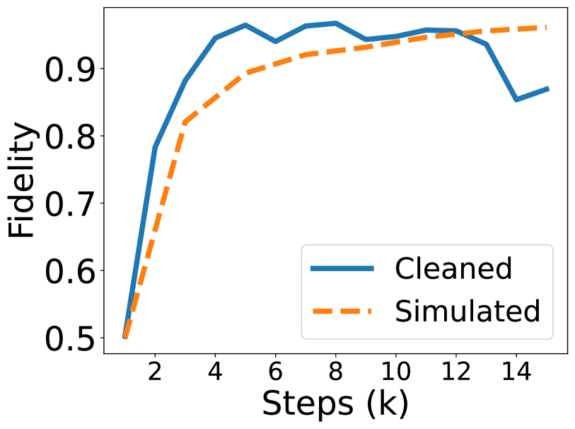
1

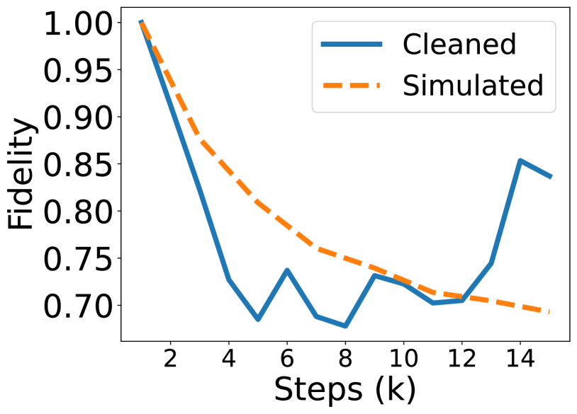
2

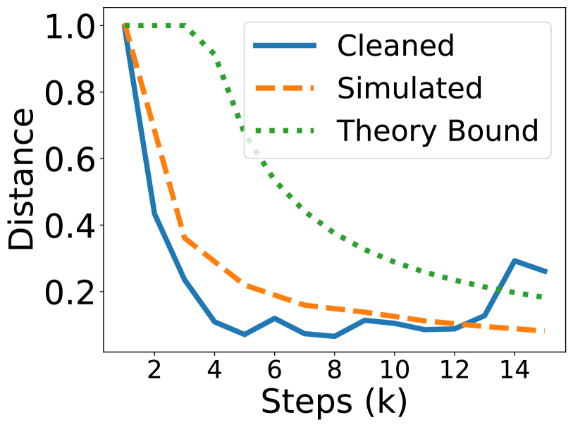
3

Figure 3: Plots of de-noised data for qubit $B$ undergoing the channel described by Equation (10). (1) Process fidelity (similarity) of channel with non-decaying identity. (2) Process fidelity with fully decayed fixed point. (3) Diamond norm distance from non-decaying identity with theoretical bound from Equation (11).

we recall the analogy between the generalized Zeno effect [35, 36], which describes continuous processes frequently interrupted by discrete channels, and the adiabatic Theorem [15], in which a fast, continuous process suppresses some aspects of a simultaneous, slower, continuous process. In this Section, we experimentally observe how the generalized Zeno effect causes depolarizing noise to self-restrict.

We consider the channel given by

$$\Phi_{(k)}=(\mathcal{E}_{0}\circ\Phi_{ZX(\pi/(2k))})^{k}\circ\mathcal{E}_{0}\hskip 2.84544pt.$$ (10)

This channel is analogous to Equation (4) in our simplified numerical example, but replacing the continuous noise by discrete interruptions. Since a rotation of $\pi/2$ corresponds to a fully entangling gate, we take a total possible rotation of $\pi/2$. The number of interruptions is $k$. Combining Equation (4) with a bound derived from Proposition B.5 and Lemma B.7 in the Supplementary Information, a tightened special case of Theorem III.8, we calculate theoretically that

$$\big{\|}\Phi_{(k)}-\mathcal{E}_{0}\big{\|}_{\Diamond}\leq\min\Big{\{}\frac{\pi^{2}}{4k}e^{\pi/2k},1.0\Big{\}}\hskip 2.84544pt.$$ (11)

Overall, we observe the predicted phenomenon: as $k$ increases, qubit $B$ is protected from interactions with the frequently depolarized qubit $A$. The real experiment appears to converge to protective Zeno dynamics more quickly than its simulated, noiseless counterpart, as seen in Figures 3.(1) and 3.(3). The accelerated convergence is potentially explainable by a small but $k$-independent under-rotation in each instance of $\Phi_{ZX(t)}$, which compounds with increasing $k$.

Comparing the experimental results shown in Figure 3 to theory and simulation, we see qualitative agreement. Since Equation (11) is intended as an upper bound, not a prediction of the experimental value, we do not necessarily expect quantitative agreement. We do see that the experimental value exceeds the ideal upper bound at large step number, which probably reflects the prevalence of real hardware noise that is not part of our model. Primarily, the experiment illustrated in Figure 3 demonstrates how what appears to be more depolarizing noise applied can reduce ultimate mixture in an interacting system. This example is analogous to the preceding, continuous scenarios, in which directly tuning up the noise rate protected neighboring qubits. Though intended to support theoretical and numerical results, this experiment may be of independent interest as a counter-intuitive consequence of the generalized Zeno effect.

To bypass unintended noise, we apply a principle inspired by error mitigation. In our scenario, an analogous procedure is greatly simplified by the fact that most forms of device noise do not resemble dephasing in the $X$ basis. Given a $4\times 4$ Choi matrix $M$ from process tomography on a single qubit, one may model the effect of incoherently applying the $X$ operator by

$$\frac{|M_{14}|+|M_{23}|}{|M_{14}|-|M_{23}|}=\exp(\chi t)\hskip 2.84544pt,$$ (12)

where $\chi\in\mathbb{R}^{+}$ is a parameter controlling the strength of $X$-basis dephasing noise. One may see via the “$D^{4}$” model introduced in [47] that a combination of $Z$-basis dephasing, amplitude damping, depolarizing, and coherent phase drift do not directly affect the ratio given in Equation (12). Hence we may extract the expected effect of $\Phi_{(k)}$ independently from common forms of noise in superconducting qubits. To extract the Zeno effect from the noise induced by real hardware, we solve for $\chi$ as in Equation (12) via the Choi matrix from process tomography, then use $\chi$ to construct a purely dephasing channel. See Section D in the Supplementary Information for more details on inferring different contributions to noise.

V Conclusions and Further Open Problems

Our results extend extend decay theory from processes with GNS detailed balance to those combining unitary with dissipative dynamics. Often bypassing detailed balance entirely, we derive results based on assumed decay properties of the dissipative part, usually weaker assumptions than GNS detailed balance. Nonetheless, a long-running problem in semigroup theory is to understand the most general class of canonical dissipator [13]. In this paper, we focus on how adding a Hamiltonian affects decay rate. It remains open whether there exist canonically dissipative (having no extractable, non-trivial Hamiltonian part), finite-dimensional generators that do not decay states to a fixed point subspace or do so slower than exponentially.

We observe via Theorem III.5 a discrepancy between continuous and discrete processes, demonstrating the role of continuous time in forestalling CMLSI-like decay. The restriction to unitality in Theorem III.5 ensures that coherent dynamics ultimately commute with projection to the overall fixed point subspace, so the fixed point subspace of the dissipative component is always at least as large as that of the combined process. Such an assumption is potentially violated, for instance, when amplitude damping co-occurs with rotations out of the computational basis. Furthermore, initial relative entropy is unbounded for fixed point states with arbitrarily small components. These complications naturally extend to those encountered with non-Markovian processes. In full generality, changing unitary dynamics might preclude any meaningful notion of a fixed point or invariant state space, requiring a different formulation of decay.

In none of the scenarios considered herein do we directly observe coherent dynamics suppressing dissipative noise. Failure of CMLSI results not from suppression of noise, but from initial noise leaving a larger subspace invariant than does the eventual decay. In self-restriction, noise quickly dissipates an initially exposed subsystem or basis, but impedes its own spread, protecting other subsytems. A natural follow-up question is whether coherent dynamics do suppress noise more directly as well. One may observe via Taylor expansion that a Hamiltonian does not suppress first order relative entropy decay via dissipative Lindbladian terms. Explicitly modeling system-environment interaction Hamiltonians, however, suggests that coherent dynamics can suppress noise, relating the Zeno effect with the noise reduction technique known as dynamical decoupling [19, 20]. Future work may address scenarios in which a natural or a priori desirable process may automatically resist environmental interactions. As this level of modeling contains an explicit, time-varying environment state, it is no longer within the usual setting of quantum Markov semigroups or dissipative subprocesses. Therefore, we expect substantially different formulations and methods to apply.

VI Acknowledgements

We thank John Smolin and Marius Junge for helpful feedback. NL is supported by the IBM Postdoc program at the Chicago Quantum Exchange. We acknowledge the use of IBM Quantum services for this work. In this paper we used ibm_lagos, which is one of the IBM Quantum Falcon Processors. The views expressed are those of the authors, and do not reflect the official policy or position of IBM or the IBM Quantum team.

The authors declare no competing interests.

VII Data and Code Availability

All data that support the plots within this paper and other findings of this study are available from the corresponding author upon reasonable request for uses compatible with the IBM Quantum End User Agreement.

Code used for the experimental and numerical portions of this paper is available from the corresponding author upon reasonable request.

Appendix A Mathematical Background

A.1 Distance and Entropy Measures

We recall the quantum relative entropy given by

$$D(\rho\|\sigma):=\text{tr}(\rho\log\rho-\rho\log\sigma)\hskip 2.84544pt.$$

for two densities $\rho,\sigma\in\mathcal{D}(\mathcal{H})$ and introduced by Umegaki [48]. Beyond tracial settings, the relative entropy has a more general definition via Tomita-Takesaki modular theory. The logarithm base does not matter when comparing ratios or asymptotic orders, so many inequalities herein need not explicitly specify a base. We will by default denote “$\log$” with base 2 for compatibility with the experimental conventions in Section IV, and “$\ln$” for the natural logarithm.

For a quantum channel (completely positive, trace-preserving map) $\Phi$, we denote by $\Phi^{*}$ the adjoint of $\Phi$ with respect to the trace (a completely positive, unital map).

By $\rho\geq\sigma$, we mean that $\rho$ is greater than $\sigma$ in the Loewner order: $\rho-\sigma$ is a non-negative matrix. We say for a pair of quantum channels $\Phi,\Psi:\mathcal{D}(\mathcal{H})\rightarrow\mathcal{D}(\mathcal{H})$ that $\Psi\geq_{cp}\Phi$ iff

$$(\Psi\otimes\hat{1}^{B})(\rho)\geq(\Psi\otimes\hat{1}^{B})(\rho)$$

for all input densities $\rho$ and finite-dimensional auxiliary systems $B\cong\mathbb{M}_{n}$ such that $n\in\mathbb{N}$. We call this and the associated symbols $<_{cp},\leq_{cp}$, and $>_{cp}$ cp-order relations. Via the Choi-Jamiolkowski isomorphism, a finite-dimensional quantum channel is fully defined by its action on one side of a maximally entangled state between its input space and an auxiliary space of the same dimension. Hence if $\Phi\geq_{cp}(1-\epsilon)\Psi$, then $\Phi=(1-\epsilon)\Psi+\epsilon\Theta$ for some $\epsilon\in(0,1)$ and other channel $\Theta$.

We denote the Schatten norms $\|\cdot\|_{p}$ for $p\in[0,\infty]$. The trace distance is given by

$$d_{tr}(\rho,\sigma):=\frac{1}{2}\|\rho-\sigma\|_{1}\hskip 2.84544pt.$$

In general, for a pair of Banach spaces $\mathcal{A}$ and $\mathcal{B}$ with respective norms $\|\cdot\|_{\mathcal{A}}$ and $\|\cdot\|_{\mathcal{B}}$, the $\mathcal{A}\rightarrow\mathcal{B}$ norm on maps from $\mathcal{A}$ to $\mathcal{B}$ is given by

$$\|\Phi\|_{\mathcal{A}\rightarrow\mathcal{B}}:=\sup_{\rho\in\mathcal{A}}\frac{\|\Phi(\rho)\|_{\mathcal{B}}}{\|\rho\|_{\mathcal{A}}}\hskip 2.84544pt.$$

For von Neumann algebras of the same type $\mathcal{A}$ and $\mathcal{B}$, we denote $\|\Phi\|_{\mathcal{A}\rightarrow\mathcal{B},cb}:=\sup_{\mathcal{C}}\|\Phi\otimes\hat{1}^{C}\|_{\mathcal{A}\otimes\mathcal{C}\rightarrow\mathcal{B}\otimes\mathcal{C}}$, where $\mathcal{C}$ is an extension over von Neumann algebras of the same type as $\mathcal{A}$ and $\mathcal{B}$ with a compatible norm in each tensor product. We denote $\|\Phi\|_{p\rightarrow q,cb}=\|\Phi\|_{\mathcal{A}\rightarrow\mathcal{B},cb}$ in which $\|\cdot\|_{\mathcal{A}}=\|\cdot\|_{p}$ and $\|\cdot\|_{\mathcal{B}}=\|\cdot\|_{q}$. The diamond norm on a map $\Phi$ is defind as $\|\Phi\|_{\Diamond}:=\|\Phi\|_{1\rightarrow 1,cb}$. We call a map $\Phi$ an $\mathcal{A}\rightarrow\mathcal{B}$ contraction if $\|\Phi\|_{\mathcal{A}\rightarrow\mathcal{B}}\leq 1$. When $\Phi$ is a map from a normed Banach space $\mathcal{A}$ to itself, we denote $\|\Phi\|:=\|\Phi\|_{\mathcal{A}\rightarrow\mathcal{A}}$.

When $\mathcal{E}$ is the conditional expectation to the fixed point subspace of a Lindbladian with detailed balance, we note the following properties:

1. $\mathcal{E}$ is idempotent (hence a projection).

2. $\mathcal{E}$ is self-adjoint with respect to the GNS inner product for $\omega$.

3. $\mathcal{E}$ has the following bimodule property: for any $a,b\in\mathcal{N}$ and $x\in\mathbb{B}(\mathcal{H})$, $\mathcal{E}^{*}(axb)=a\mathcal{E}^{*}(x)b$. Following, for any density $\rho\in\mathcal{D}(\mathcal{H})$, $\mathcal{E}(a\rho b)=a\mathcal{E}(\rho)b$.

Appendix B Generalized Zeno Effect and Entropy Decay

Much of this Section is devoted to a technical reanalysis of the generalized Zeno effect. Rather than spectral properties of the channels involved, we base our estimates on cp-order inequalities and seek comparability with CMLSI and $\lambda$-decay. The bounds derived herein are nonetheless in terms of norms as described in Appendix A. These bounds are in principle very general, requiring only sub-multiplicativity of $\|\cdot\|_{\mathcal{A}\rightarrow\mathcal{B}}$ in addition to its being a norm. A restriction, however, is that many of the results must assume contractivity of most or all maps involved. The diamond norm is especially convenient in this sense, as channels automatically satisfy this assumption. The diamond norm is however only obviously usable in algebras with a finite trace, which extends it to some but not all infinite-dimensional settings. In principle, one could apply results herein using the Kosaki norms [49] in all von Neumann algebras, but more care would be needed to ensure contractivity of involved maps and in some cases boundedness and analyticity. Since the purpose of this paper is however to understand the relationship between the Zeno effect and mostly finite-dimensional semigroup theory, we will not be too concerned with technical barriers in non-tracial settings. For infinite-dimensional versions of the generalized Zeno effect, see [37, 38].

To simplify notation, let

$$F^{({m})}_{{a}}:=\frac{a^{m}\exp(a)}{m!}$$ (13)

for any scalar $a>0$, $k\in\mathbb{N}$.

Remark B.1.

For any $a>0$ such that $\exp(a)$ equals its Taylor series,

$$\exp(a)-\sum_{n=0}^{k}\frac{a^{n}}{n!}=\sum_{n={k+1}}^{\infty}\frac{a^{n}}{n!}=a^{k+1}\sum_{n=0}^{\infty}\frac{a^{n}}{(n+k+1)!}\leq\frac{a^{k+1}\exp(a)}{(k+1)!}=F^{({k+1})}_{{a}}\hskip 2.84544pt.$$

Lemma B.2.

Let $\mathcal{L}$, and $\mathcal{E}$ be respectively a Lindbladian and a map on the same von Neumann algebra. Let $\mathcal{A}$ be a normed input subspace that is preserved by $\mathcal{L}$, and $\mathcal{B}$ be the normed output space of $\mathcal{E}$. Then for any $t\in\mathbb{R}$

$$\Big{\|}\mathcal{E}\circ\sum_{m=k}^{\infty}\frac{(it)^{m}}{m!}\mathcal{L}^{m}\Big{\|}_{\mathcal{A}\rightarrow\mathcal{B},(cb)}\leq F^{({k})}_{{\|\mathcal{L}\|_{\mathcal{A},(cb)}t}}\|\mathcal{E}\|_{\mathcal{A}\rightarrow\mathcal{B},(cb)}\hskip 2.84544pt.$$

Proof.

First, we name a given input $\rho$ and use the triangle inequality to separate terms.

$$\begin{split}\Big{\|}\mathcal{E}\circ\sum_{m=k}^{\infty}\frac{(it)^{m}}{m!}\mathcal{L}\Big{\|}_{\mathcal{A}\rightarrow\mathcal{B},(cb)}\leq\sum_{m=k}^{\infty}\frac{t^{m}}{m!}\|\mathcal{E}\circ\mathcal{L}^{m}\|_{\mathcal{A}\rightarrow\mathcal{B},(cb)}\hskip 2.84544pt.\end{split}$$ (14)

We then consider each term.

$$\|\mathcal{E}\circ\mathcal{L}^{m}(\rho)\|_{\mathcal{A}\rightarrow\mathcal{B},(cb)}\leq\|\mathcal{E}\|_{\mathcal{A}\rightarrow\mathcal{B},cb}\|\mathcal{L}^{m}(\rho)\|_{\mathcal{A},(cb)}\hskip 2.84544pt.$$

The proof then follows from Remark B.1. ∎

Lemma B.3.

Let $(f_{m})_{m=1}^{k},(g_{m})_{m=1}^{k}$ be families of maps for $k\in\mathbb{N}$ such that $f_{m}\circ f_{m-1}$ and $g_{m}\circ g_{m-1}$ are valid compositions. Let $\omega_{l}=\prod_{m=1}^{l}f_{m}(\rho)$ for input $\rho$ and each $l\in 1...k$. Then

$$\bigg{(}\prod_{m=1}^{k}f_{m}-\prod_{m=1}^{k}g_{m}\bigg{)}(\rho)=\sum_{l=1}^{k}\Big{(}\prod_{n=l+1}^{k}g_{n}\Big{)}(f_{l}-g_{l})(\omega_{l-1})\hskip 2.84544pt.$$

Proof.

For each value of $l$,

$$\Big{(}\prod_{n=l+1}^{k}g_{n}\Big{)}(\omega_{l})-\Big{(}\prod_{n=l}^{k}g_{n}\Big{)}(\omega_{l-1})=\Big{(}\prod_{n=l+1}^{k}g_{n}\Big{)}(f_{l}-g_{l})(\omega_{l-1})\hskip 2.84544pt.$$

The Lemma then follows from induction. ∎

Corollary B.4.

Let $(f_{m})_{m=1}^{k},(g_{m})_{m=1}^{k}$ be families of maps as in Lemma B.3 from a submultiplicatively normed Banach space to itself. Then

$$\bigg{\|}\prod_{m=1}^{k}g_{m}-\prod_{m=1}^{k}f_{m}\bigg{\|}\leq\sum_{l=0}^{k-1}\bigg{\|}\prod_{n=l+1}^{k}g_{n}\bigg{\|}\bigg{\|}\prod_{n=1}^{l-1}f_{n}\bigg{\|}\|f_{l}-g_{l}\|\hskip 2.84544pt.$$

Proof.

We apply Lemma B.3 to the normed quantity in the left hand side, obtaining that

$$\bigg{\|}\prod_{m=1}^{k}g_{m}-\prod_{m=1}^{k}f_{m}\bigg{\|}=\sup_{\rho}\frac{1}{\|\rho\|}\bigg{\|}\sum_{l=1}^{k}\Big{(}\prod_{n=l+1}^{k}g_{n}\Big{)}(f_{l}-g_{l})\Big{(}\prod_{m=1}^{l-1}f_{m}\Big{)}(\rho)\bigg{\|}\hskip 2.84544pt.$$

Via the triangle inequality, we may separate the terms in the sum. We then split the product via submultiplicativity. The overall supremum over $\rho$ then underestimates the per-term and per-factor suprema, completing the Corollary. ∎

B.1 Results for Interruptions by Conditional Expectations

Here we consider a continuous process interrupted by a conditional expectation. The results of this Subsection underpin the the theory bound in Subsection IV recalled as Equation (11). Furthermore, they show in a relatively simple calculation how Zeno-like bounds arise from Taylor expansion and norm comparison. These calculations may guide the intuition for the more complicated results of Subsection B.2.

Proposition B.5.

Let $\mathcal{L}$ and $\mathcal{E}$ be respectively a Lindbladian and projection to the subspace $\mathcal{N}\subseteq\mathcal{A}$ defined on Banach space $\mathcal{A}$ such that $\exp(-\mathcal{L})$ is equal to its Taylor series. Let $(t_{m})_{m=1}^{k}$ be a family of values in $\mathbb{R}^{+}$ such that $t_{m}=O(1/k)$. Let $t=\sum_{m}t_{m}$. Then

$$\begin{split}&\Big{\|}\prod_{m=1}^{k}(\mathcal{E}\exp(-\mathcal{L}t_{m})\mathcal{E})-\exp(-t\mathcal{E}\circ\mathcal{L}\circ\mathcal{E})\Big{\|}_{\mathcal{N}\rightarrow\mathcal{N},(cb)}=O(1/k)\\ &\leq\sum_{m=1}^{k}\big{(}\|\mathcal{E}\|_{\mathcal{A}\rightarrow\mathcal{N},(cb)}F^{({2})}_{{t_{m}\|\mathcal{L}\|_{\mathcal{A}\rightarrow\mathcal{A},(cb)}}}+F^{({2})}_{{t_{m}\|\mathcal{E}\mathcal{L}\mathcal{E}\|_{\mathcal{N}\rightarrow\mathcal{N},(cb)}}}\big{)}\Big{\|}\exp\Big{(}-\mathcal{E}\mathcal{L}\mathcal{E}\sum_{n=m+1}^{k}t_{n}\Big{)}\Big{\|}_{\mathcal{N}\rightarrow\mathcal{N},(cb)}\hskip 2.84544pt.\end{split}$$

Proof.

First, we show for one value of $t$ that

$$\|\mathcal{E}\exp(-\mathcal{L}t)\mathcal{E}(\rho)-\exp(-t\mathcal{E}\circ\mathcal{L}\circ\mathcal{E})\mathcal{E}\|_{\mathcal{N}\rightarrow\mathcal{N},(cb)}\leq\big{(}F^{({2})}_{{\|\mathcal{L}\|_{\mathcal{N}\rightarrow\mathcal{A}}t}}+F^{({2})}_{{\|\mathcal{E}\circ\mathcal{L}\circ\mathcal{E}\|_{\mathcal{N}\rightarrow\mathcal{A},(cb)}t}}\big{)}\hskip 2.84544pt.$$ (15)

For any input $\rho$, one may Taylor expand

$$\begin{split}(\mathcal{E}\circ\exp(-\mathcal{L}t)\circ\mathcal{E})(\rho)=\mathcal{E}(\rho)-t\mathcal{E}(\mathcal{L}(\mathcal{E}(\rho)))+\mathcal{E}\Big{(}\sum_{m=2}^{\infty}\frac{(-t)^{m}}{m!}\mathcal{L}^{m}(\mathcal{E}(\rho))\Big{)}\end{split}$$ (16)

The terms up to first order in $t$ match those of $\exp(-t\mathcal{E}\circ\mathcal{L}\circ\mathcal{E})$. Via the triangle inequality and idempotence of $\mathcal{L}$, what remains is to bound the distance of higher order terms,

$$\Big{\|}\mathcal{E}\Big{(}\sum_{m=2}^{\infty}\frac{(-t)^{m}}{m!}\mathcal{L}^{m}(\mathcal{E}(\rho))-\sum_{m=2}^{\infty}\frac{(-t)^{m}}{m!}(\mathcal{E}\circ\mathcal{L}\circ\mathcal{E})^{m}(\mathcal{E}(\rho))\Big{)}\Big{\|}_{\mathcal{N}\rightarrow\mathcal{N},(cb)}\hskip 2.84544pt.$$

We apply Lemma B.2 to each higher-order sequence individually, using the triangle inequality to separate them. This step completes the proof of Equation (15).

We then apply Corollary B.4. The fact that $\exp(a)\exp(b)=\exp(a+b)$ whenever $[a,b]=0$ completes the Proposition. ∎

Proposition B.5 simplifies when bounding the diamond norm, because quantum channels are contractions. Hence

$$\Big{\|}\prod_{m=1}^{k}(\mathcal{E}\exp(-\mathcal{L}t_{m}/k)\mathcal{E})-\exp(-t\mathcal{E}\circ\mathcal{L}\circ\mathcal{E})\circ\mathcal{E}\Big{\|}_{\Diamond}\leq\sum_{m=1}^{k}\big{(}F^{({2})}_{{t_{m}\|\mathcal{L}\|_{\Diamond}/k}}+F^{({2})}_{{t_{m}\|\mathcal{E}\mathcal{L}\mathcal{E}\|_{\Diamond}/k}}\big{)}\hskip 2.84544pt.$$ (17)

Proposition B.5 yields additional simplifications when $\mathcal{L}$ has the form of a Hamiltonian:

Remark B.6.

When $\mathcal{E}$ is a conditional expectation and $\mathcal{L}=i[H,\cdot]$ for some Hamiltonian $H$, the bimodule property of conditional expectations implies that for any input $\rho$,

$$\mathcal{E}(i[H,\mathcal{E}(\rho)])=i\mathcal{E}(H\mathcal{E}(\rho))-i\mathcal{E}(\mathcal{E}(\rho)H)=i[\mathcal{E}(H),\mathcal{E}(\rho)]\hskip 2.84544pt.$$ (18)

Lemma B.7.

For any $p$ such that $\|\cdot\|_{p\rightarrow p}$ is a norm and $\|\cdot\|_{p}$ obeys Hölder’s inequality,

$$\|[H,\cdot]^{m}\|_{p\rightarrow q,(cb)}\leq 2^{m}\|H\|_{\infty}^{m}\sup_{\rho}\|\rho\|_{q}/\|\rho\|_{p}$$

Proof.

For Hamiltonians, we use the fact that $[H,\cdot]^{m}(\rho)$ generates $2^{m}$ terms on any density $\rho$, each of which contains $m$ powers of $H$ and one of $\rho$. Using Hölder’s inequality and its inductive generalization,

$$\|H^{k}\rho H^{m-k}\|_{p}\leq\|H^{k}\|_{\infty}\|\rho H^{m-k}\|_{p}\leq\|H^{k}\|_{\infty}\|\|\rho\|_{p}\|H^{m-k}\|_{\infty}\leq\|\rho\|_{p}\|H\|_{\infty}^{m}$$

for any integer $k$ such that $0\leq k\leq m$. Hence

$$\|[H,\cdot]^{m}\|_{p\rightarrow p}=\sup_{\rho}\|[H,\cdot]^{m}(\rho)\|_{p}/\|\rho\|_{p}\leq 2^{m}\|H\|_{\infty}^{m}\hskip 2.84544pt.$$

To conclude the Lemma, we return to Equation (14) and re-assemble the exponential series, using Remark B.1. ∎

B.2 Results for Maps Converging to Fixed Points

Here we show Zeno-like effects for both discrete channels compositions and Lindbladian-generated semigroups that converge toward a fixed point projection $\mathcal{E}$. Generalizing the results of the previous Section, those of this Section no longer assume that the interruption is itself a projection.

Lemma B.8.

Let $(\Phi_{m})_{m=1}^{k}$ be a family of bounded maps on Banach space $\mathcal{A}$. Let $(\mathcal{L}_{m})_{m=1}^{k}$ be a family of bounded Lindbladians. Let $t_{1},...,t_{k}\in\mathbb{R}^{+}$. Then

$$\bigg{\|}\prod_{m=1}^{k}(\Phi_{m}\circ e^{-\mathcal{L}_{m}t_{m}})-\prod_{m=1}^{k}(\Phi_{m}\circ(1-\mathcal{L}_{m}t_{m}))\bigg{\|}\leq\sum_{r=1}^{k}\bigg{\|}\prod_{m=r+1}^{k}\Phi_{m}e^{-\mathcal{L}_{m}t_{m}/k}\bigg{\|}F^{({2})}_{{\|\mathcal{L}_{m}\|t_{r}}}\hskip 2.84544pt.$$

Proof.

The Lemma follows from noting that $(1-\mathcal{L}t)$ is the 1st order Taylor expansion of $e^{-\mathcal{L}t}$ for any $t\in\mathbb{R}^{+}$, so

$$\|e^{-\mathcal{L}_{m}t_{m}}-(1-\mathcal{L}t_{m})\|\leq F^{({2})}_{{\|\mathcal{L}_{m}\|t_{m}}}$$

for each $m\in 1...k$. Corollary B.4 completes the Lemma. ∎

While it is often intuitive to think of a Lindbladian as having units of inverse time and appearing alongside a time parameter in the expression $\exp(-\mathcal{L}t)$, $t$ is formally redundant in many of the mathematical expressions we will use. When $t$ is an overall parameter (not changing by interval as in Lemma B.8), we may instead write $\exp(-\mathcal{L})$, implicitly absorbing $t$ as a multiplying factor in $\mathcal{L}$. Doing so simplifies notation, and one may trivially re-extract the parameter $t$ by substituting $\mathcal{L}\rightarrow t\mathcal{L}$ in resulting expressions.

Subsequent Lemmas require some combinatoric notation. For $m<k\in\mathbb{N}$, let

$$WS(m,k)\subset\{[l_{1},...,r_{1}],...,[l_{m},...,r_{m}]:1=l_{1}\leq r_{1}<l_{2}\leq r_{2}...<l_{m}\leq r_{m}=k\}$$

denote the set of partitions of $k$ into $m$ contiguous, ordered, non-overlapping intervals. For given $W\in WS(m,k)$, let $W(j)$ denotes a contiguous sequence of indices for $j\in 1...m$. Let $|W(j)|$ denote the number of indices in $W(j)$, which we will refer to as its length. By $W(j)[l]$ we denote the $l$th index in $W(j)$ for $l\in 1...|W(j)|$. As an example, we might take $W=(1\mapsto[1,2,3],2\mapsto[4,5])\in WS(2,5)$, in which case $W(1)=[1,2,3],W(2)=[4,5]$, and $W(2)[1]=4$. In this example, we would have $l_{1}=1,r_{1}=3,l_{2}=4,r_{2}=5$.

For any $n\leq k$, let $WS(m,k,n)\subseteq WS(m,k)$ denote the subset of partitions such that $|W(j)|\geq n$ for all $j\in 1...m$. Note that $WS(m,k,n)$ is the empty set whenever $n>k/m$.

Lemma B.9.

Let $(\Phi_{m})_{m=1}^{k}$ be a family contractions on a Banach space for any $k\in\mathbb{N}$. Let $(\mathcal{L}_{m})_{m=1}^{k}$ be bounded Lindbladians such that $e^{-\mathcal{L}_{m}}$ is also contractive for each $m$. Let $\|\mathcal{L}\|:=\max_{m}\{\|\mathcal{L}_{m}\|\}$. Then for any $\alpha:\mathbb{N}\rightarrow(1/k,1)$ and $n\in 1...k$,

$$\begin{split}&\bigg{\|}\prod_{m=1}^{k}\Big{(}\Phi_{m}\Big{(}1-\frac{\mathcal{L}_{m}}{k}\Big{)}\Big{)}-\sum_{m=0}^{n}\frac{(-1)^{m}}{k^{m}}\sum_{W}\prod_{j=1}^{m}(\Phi_{W(j)}\mathcal{L}_{W,j})\Phi_{W(m+1)}\bigg{\|}\\ &\leq\sum_{m=1}^{n}\frac{\alpha(m)m\|\mathcal{L}\|^{m}}{(1-m)!}+\sum_{m=n+1}^{k}\frac{\|\mathcal{L}\|^{m}}{m!},\end{split}$$ (19)

where $\Phi_{W(j)}=\Phi_{W(j)[|W(j)|],k}\circ...\circ\Phi_{W(j)[1],k}$, and the sum over $W$ is within the set $WS(m+1,k,\alpha(m)k)$, and each $\mathcal{L}_{W,j}\in(\mathcal{L}_{m})$ is the Lindbladian appearing between the partitions $W(j)$ and $W(j+1)$.

Proof.

For convenience of notation, let the norm distance in this Lemma be denoted $\Delta$.

The first step is the binomial expansion, where we substitute the index $r$ for $m$ on the left hand side,

$$\prod_{r=1}^{k}(\Phi_{r}(1-\mathcal{L}_{m}/k))=\sum_{m=0}^{k}\frac{(-1)^{m}}{k^{m}}\sum_{W\in WS(m+1,k)}\Big{(}\prod_{j=1}^{m}(\Phi_{W(j)}\mathcal{L}_{W,j})\Big{)}\Phi_{W(m+1)}\hskip 2.84544pt.$$ (20)

We see that the right hand side of Equation (20) is the same as that in the compared quantity from the desired inequality, except that the latter sums over $WS(m+1,k,\alpha(l)k)$ instead of over $WS(m+1,k)$. Hence we must bound the number and magnitude of terms containing short partitions.

Assume we are given some function $\alpha:\mathbb{N}\rightarrow\mathbb{R}^{+}$ and consider a particular value of $m$ as in Equation (20). The number of partitions containing at least one segment of length at most length $\alpha(m)k$ is upper-bounded by $(k\text{ choose }m-1)\times(2\lceil\alpha(m)mk\rceil\text{ choose }1)/2$, since we can consider first placing $m-1$ partition boundaries within $k$ locations, then choose a final partition boundary that is no more than $\alpha(m)k$ indices away from one of the $m-1$ original boundaries or from first or last index. The divisor of 2 arises from the invariance under exchange between the final boundary and its close neighbor. This bound is an overcount, since the first $m-1$ placements might already contain one or more partitions that are too small. We will ignore this overcounting, since for $k/m>>\alpha(m)k$, it is not expected to contribute much. Using the triangle inequality to recombine the sum in Equation (20),

$$\Delta\leq\sum_{m=0}^{k}\frac{\|\mathcal{L}\|^{m}}{k^{m}}\binom{k}{m-1}\lceil\alpha(m)mk\rceil\hskip 2.84544pt.$$

It is easy to see that $(k\text{ choose }m-1)\leq k(k-1)^{m-2}/(m-1)!$. We then observe that $(k-1)/k\leq k/(k+1)$ and that $\lceil\alpha(m)mk\rceil\leq\alpha(m)m(k+1)$. Hence for $m\leq n$,

$$\ \frac{k(k-1)^{m-2}\lceil\alpha(m)mk\rceil}{k^{m}(m-1)!}\leq\frac{\alpha(m)m}{(1-m)!}$$

We then separately handle the terms with $m>n$. Returning to Equation (20), we apply the coarse bound that the cardinality $|WS(m+1,k)|\leq(k\text{ choose }m)\leq k^{m}/m!$. Hence

$$\bigg{\|}\sum_{m=n+1}^{k}\frac{(-1)^{m}}{k^{m}}\sum_{W\in WS(m+1,k)}\prod_{j=1}^{m}(\Phi_{W(j)}\mathcal{L}_{W,j})\Phi_{W(m+1)}\bigg{\|}\leq\sum_{m=n+1}^{k}\frac{\|\mathcal{L}\|^{m}}{m!}\hskip 2.84544pt.$$

∎

Lemma B.10.

Let $(\Phi_{m})_{m=1}^{k}$ and $(\mathcal{L}_{m})_{m=1}^{k}$ be as in Lemma B.9 with the additional assumption that for given $r\in\mathbb{N}$ and $\gamma\in(0,k]$, $\Phi_{W(j)}\geq_{cp}(1-\epsilon)\mathcal{E}$ whenever $|W(j)|\geq k/\gamma$. Then

$$\begin{split}&\bigg{\|}\sum_{m=0}^{k}\frac{(-1)^{m}}{k^{m}}\sum_{W\in WS_{k}}\prod_{j=1}^{m}(\Phi_{W(j)}\mathcal{L}_{W,j})\Phi_{W(m+1)}-\sum_{m=0}^{k}\sum_{W\in WS_{k}}\frac{(-1)^{m}}{k^{m}}\prod_{j=1}^{m}(\mathcal{E}\mathcal{L}_{W,j}\mathcal{E})\bigg{\|}\\ &\hskip 2.84544pt\leq\epsilon^{\lfloor\gamma/r\rfloor}\|\mathcal{L}\|\exp(\|\mathcal{L}\|)+\sum_{m=r}^{k}\frac{\|\mathcal{L}\|^{m}}{(m-1)!}\hskip 2.84544pt,\end{split}$$

where $WS_{k}:=WS(m+1,k,\lfloor k/m\rfloor)$ in the sums, and $\|\mathcal{L}\|:=\max_{m}\|\mathcal{L}_{m}\|$.

Proof.

We first consider the terms for individual values of $m\leq k$, rewriting

$$\sum_{W}\prod_{j=1}^{m}(\Phi_{W(j)}\mathcal{L}_{W,j})\Phi_{W(m+1)}=\sum_{W}\prod_{j=1}^{m}(((1-\epsilon_{m})\mathcal{E}+\epsilon_{m}\Psi_{W(j)})\mathcal{L}_{W,j})((1-\epsilon_{m})\mathcal{E}+\epsilon_{m}\Psi_{W(m+1)})$$

for some maps $\{\Psi_{W(j)}:j=1...m+1\}$ such that $\mathcal{E}\Psi_{W(j)}=\Psi_{W(j)}\mathcal{E}=\mathcal{E}$. Here $W\in WS(m+1,k,\lfloor k/m\rfloor)$, and $\epsilon_{m}=\epsilon^{\lfloor\gamma/m\rfloor}$. We estimate the distance

$$\begin{split}&\Big{\|}\prod_{j=1}^{m}(((1-\epsilon_{m})\mathcal{E}+\epsilon_{m}\Psi_{W(j)})\mathcal{L}_{W,j})((1-\epsilon_{m})\mathcal{E}+\epsilon_{m}\Psi_{W(m+1)})-\prod_{j=1}^{m}(-\mathcal{E}\mathcal{L}_{W,j}\mathcal{E})\Big{\|}\\ &\hskip 2.84544pt\hskip 2.84544pt\leq\|\mathcal{L}\|^{m}\big{(}1-(1-\epsilon^{\lfloor\gamma/r\rfloor})^{m}\big{)}\end{split}$$

for a single value of $W$. This bound follows from the number of $\mathcal{E}$ vs. $\Psi_{W(j)}$ being binomially distributed in the first term after expanding, since the compared expressions match when the former contains only $\mathcal{E}$ and $\mathcal{L}$ factors. When $m=0$, the inequality is trivial. Via Bernoulli’s inequality, we simplify the expression for $m>0$ to $(1-(1-\epsilon^{\lfloor\gamma/m\rfloor})^{m}\big{)}\leq m\epsilon^{\lfloor\gamma/m\rfloor}$. Hence

$$\begin{split}&\Big{\|}\sum_{m=0}^{k}\frac{1}{k^{m}}\sum_{W}\prod_{j=1}^{m}(((1-\epsilon_{m})\mathcal{E}+\epsilon_{m}\Psi_{W(j)})\mathcal{L}_{W,j})((1-\epsilon_{m})\mathcal{E}+\epsilon_{m}\Psi_{W(m+1)})\\ &\hskip 2.84544pt\hskip 2.84544pt\hskip 2.84544pt-\sum_{m=0}^{k}\frac{(-1)^{m}}{k^{m}}\sum_{W}\prod_{j=1}^{m}(\mathcal{E}\mathcal{L}_{W,j}\mathcal{E})\Big{\|}\leq\sum_{m=0}^{k}\frac{1}{k^{m}}\binom{k}{m}\|\mathcal{L}\|^{m}m\epsilon^{\lfloor\gamma/m\rfloor}\leq\sum_{m=0}^{k}\frac{\|\mathcal{L}\|^{m}}{m!}m\epsilon^{\lfloor\gamma/m\rfloor}\hskip 2.84544pt,\end{split}$$ (21)

where the final inequality follows from recalling that $(k\text{ choose }m)\leq k^{m}/m!$. Then

$$\sum_{m=0}^{k}\frac{\|\mathcal{L}\|^{m}}{m!}m\epsilon^{\lfloor\gamma/m\rfloor}\leq\sum_{m=0}^{r}\frac{\|\mathcal{L}\|^{m}}{m!}m\epsilon^{\lfloor\gamma/m\rfloor}+\sum_{m=r}^{k}\frac{\|\mathcal{L}\|^{m}}{(m-1)!}\hskip 2.84544pt.$$

For an overestimate, we note that $\epsilon^{\lfloor\gamma/m\rfloor}\leq\epsilon^{\lfloor\gamma/r\rfloor}$ for all $m\in 1...r$. Hence

$$...\leq\epsilon^{\lfloor\gamma/r\rfloor}\|\mathcal{L}\|\exp(\|\mathcal{L}\|)+\sum_{m=r}^{k}\frac{\|\mathcal{L}\|^{m}}{(m-1)!}\hskip 2.84544pt.$$

∎

Theorem B.11.

Let $(\Phi_{m})_{m=1}^{k}$ be a family of norm contractions for any $k\in\mathbb{N}$ all having fixed point projector $\mathcal{E}$. Let $(\mathcal{L}_{m})_{m=1}^{k}$ be bounded Lindbladians such that $e^{-\mathcal{L}_{m}s}$ is contractive for all $s\in\mathbb{R}^{+}$ and $m$. Let $\|\mathcal{L}\|:=\max_{m}\|\mathcal{L}_{m}\|$. Let $\gamma\in\mathbb{R}^{+}$ such that for any consecutive sequence $\Phi_{W}=\Phi_{j_{1}},...,\Phi_{j_{\lceil k/\gamma\rceil}}$, $\Phi_{W}\geq_{cp}(1-\epsilon)\mathcal{E}$. For any $a>0$ and $q\in 1...k$, if $\lceil a\gamma/q\log_{\epsilon}(\gamma/q)\rceil\geq\|\mathcal{L}\|/q+3$, then

$$\begin{split}\Big{\|}\prod_{m=1}^{k}\big{(}\Phi_{m}\circ e^{-\mathcal{L}_{m}/k}\big{)}-\prod_{m=1}^{k}e^{-\mathcal{E}\mathcal{L}_{m}\mathcal{E}}\Big{\|}\leq&(k+k\%q)\big{(}F^{({2})}_{{\|\mathcal{L}\|/k}}+F^{({2})}_{{\|\mathcal{E}\mathcal{L}\mathcal{E}\|/k}}\big{)}\\ &\hskip 2.84544pt+q\Big{(}\frac{q}{\gamma}(F^{({1})}_{{\|\mathcal{L}\|/q}}+\epsilon^{1/a})+\beta(a,\gamma/q,\epsilon,\|\mathcal{L}\|/q)\Big{)}\hskip 2.84544pt,\end{split}$$

where $\%$ denotes the modulus operator, and

$$\beta(a,\gamma,\epsilon,l):=\frac{1}{\sqrt{2\pi\lceil a\gamma\log_{\epsilon}(\gamma/q)\rceil}}\Big{(}\frac{el}{\lceil a\gamma\log_{\epsilon}\gamma\rceil}\Big{)}^{\lceil a\gamma\log_{\epsilon}\gamma\rceil}\hskip 2.84544pt.$$

Proof.

The Theorem follows from Lemmas B.8, B.9, and B.10 with appropriate parameters. For general convenience, note that

$$\sum_{m=r}^{k}\|\mathcal{L}\|/(m-1)!=\|\mathcal{L}\|\sum_{m=r-1}^{k-1}\|\mathcal{L}\|^{m}/m!$$ (22)

for any $r\in 1...k$.

Let $\Delta_{1}$ denote the contribution from Lemma B.8. Under the assumptions of this Theorem,

$$\Delta_{1}\leq k(F^{({2})}_{{\|\mathcal{L}\|/k}}+F^{({2})}_{{\|\mathcal{E}\mathcal{L}\mathcal{E}\|/k}})\hskip 2.84544pt.$$

Let $\Delta_{2}$ denote the contribution from Lemma B.9 with $\alpha(m)=1/\gamma m$ and $n=k$. Using Equation (22),

$$\Delta_{2}\leq\sum_{m=1}^{k}\|\mathcal{L}\|^{m}m\alpha(m)/(m-1)!=\|\mathcal{L}\|\sum_{m=0}^{k}\frac{\|\mathcal{L}\|^{m}}{\gamma m!}=\frac{1}{\gamma}F^{({1})}_{{\|\mathcal{L}\|}}\hskip 2.84544pt.$$

Consider Lemma B.10 for $r\in\mathbb{N}$. Using some series identities [50] and overestimating by replacing $k-1\rightarrow\infty$,

$$\sum_{m=r-1}^{k-1}\|\mathcal{L}\|^{m}/m!\leq e^{\|\mathcal{L}\|}\frac{\Gamma(r-1)-\Gamma(r-1,\|\mathcal{L}\|)}{\Gamma(r-1)}=\frac{e^{\|\mathcal{L}\|}}{(r-1)!}\int_{0}^{\|\mathcal{L}\|}t^{r-2}e^{t}dt\hskip 2.84544pt,$$

where $\Gamma(\cdot,\cdot)$ denotes the upper incomplete Gamma function and $\Gamma(\cdot)$ the gamma function. Assuming that $r\geq\|\mathcal{L}\|+2$, one can easily check that $t^{r-2}e^{-t}$ is increasing on the integrated region. Hence we may estimate $t^{r-2}e^{-t}\leq\|\mathcal{L}\|^{r-2}e^{-\|\mathcal{L}\|}$ over the entire integral, obtaining an upper bound of $\|\mathcal{L}\|^{r-1}e^{-\|\mathcal{L}\|}$. Via Equation (22) and Robbins’s precise form of Stirling’s approximation [51], $m!\geq\sqrt{2\pi m}(m/e)^{m}$. Hence

$$\sum_{m=r-1}^{k-1}\|\mathcal{L}\|^{m}/m!\leq\frac{1}{\sqrt{2\pi(r-1)}}\Big{(}\frac{e\|\mathcal{L}\|}{r-1}\Big{)}^{r-1}\hskip 2.84544pt.$$

Letting the contribution from Lemma B.10 be denoted $\Delta_{3}$,

$$\Delta_{3}\leq\epsilon^{\lfloor\gamma/r\rfloor}+\frac{1}{\sqrt{2\pi(r-1)}}\Big{(}\frac{e\|\mathcal{L}\|}{r-1}\Big{)}^{r-1}\hskip 2.84544pt.$$

To optimize this expression, it will be convenient to set $r=\lceil a\gamma/\log_{\epsilon}\gamma\rceil-1$, assuming $\gamma$ large enough that $r\geq\|\mathcal{L}\|+2$, and where $a>0$ is a free parameter. We then find

$$\Delta_{3}\leq\frac{\epsilon^{1/a}}{\gamma}+\frac{1}{\sqrt{2\pi\lceil a\gamma/\log_{\epsilon}\gamma\rceil}}\Big{(}\frac{e\|\mathcal{L}\|}{\lceil a\gamma/\log_{\epsilon}\gamma\rceil}\Big{)}^{\lceil a\gamma/\log_{\epsilon}\gamma\rceil}\hskip 2.84544pt.$$

Let $\Delta_{4}$ denote the contribution from again applying Lemma B.8, this time to relate the term $\sum_{m=0}^{k}(\mathcal{E}\mathcal{L}\mathcal{E})^{m}/k^{m}=(1-\mathcal{E}\mathcal{L}\mathcal{E}/k)^{k}$ to the desired $\exp(-\mathcal{E}\mathcal{L}\mathcal{E}/k)$. We find $\Delta_{4}\leq kF^{({2})}_{{\|\mathcal{E}\mathcal{L}\mathcal{E}\|/k}}$.

Via the triangle inequality, $\sum_{r=1}^{4}\Delta_{r}$ yields that

$$\begin{split}\Big{\|}\prod_{m=1}^{k}\big{(}\Phi_{m}\circ e^{-\mathcal{L}/k}\big{)}-e^{-\mathcal{E}\mathcal{L}\mathcal{E}}\mathcal{E}\Big{\|}&\leq k\big{(}F^{({2})}_{{\|\mathcal{L}\|/k}}+F^{({2})}_{{\|\mathcal{E}\mathcal{L}\mathcal{E}\|/k}}\big{)}+\frac{1}{\gamma}(F^{({1})}_{{\|\mathcal{L}\|}}+\epsilon^{1/a})\\ &+\frac{1}{\sqrt{2\pi\lceil a\gamma/\log_{\epsilon}\gamma\rceil}}\Big{(}\frac{e\|\mathcal{L}\|}{\lceil a\gamma/\log_{\epsilon}\gamma\rceil}\Big{)}^{\lceil a\gamma/\log_{\epsilon}\gamma\rceil}\hskip 2.84544pt.\end{split}$$ (23)

Finally, we introduce $q$. We may trivially re-express

$$\begin{split}&\prod_{m=1}^{k}\big{(}\Phi_{m}\circ e^{-\mathcal{L}/k}\big{)}-e^{-\mathcal{E}\mathcal{L}\mathcal{E}}\mathcal{E}\\ &\hskip 2.84544pt=\prod_{m=0}^{q-2}\Big{(}\prod_{n=1}^{k/q}\big{(}\Phi_{m(k/q)+n}\circ e^{-(\mathcal{L}/q)/(k/q)}\big{)}\Big{)}\prod_{n=1}^{k\%q}\big{(}\Phi_{m(k/q)+n}\circ e^{-(\mathcal{L}/q)/(k/q)}\big{)}-\big{(}e^{-\mathcal{E}\mathcal{L}\mathcal{E}/q}\big{)}^{q}\mathcal{E}\hskip 2.84544pt.\end{split}$$

If $q$ does not divide $k$, then we may greatly simplify and slightly loosen the bound by effectively extending the product until it does, for instance letting $\Phi_{m}=\Phi_{m\%k}$ and $\mathcal{L}_{m}=\mathcal{L}_{m\%k}$. Hence letting $\tilde{k}=k+k\%q$,

$$\begin{split}&\Big{\|}\prod_{m=1}^{k}\big{(}\Phi_{m}\circ e^{-\mathcal{L}_{m}/k}\big{)}-\prod_{m=1}^{k}e^{-\mathcal{E}\mathcal{L}_{m}\mathcal{E}}\Big{\|}\leq\Big{\|}\prod_{m=0}^{q-1}\Big{(}\prod_{n=1}^{\tilde{k}/q}\big{(}\Phi_{m(\tilde{k}/q)+n}\circ e^{-(\mathcal{L}/q)/(k/q)}\big{)}\Big{)}-\big{(}e^{-\mathcal{E}\mathcal{L}\mathcal{E}/q}\big{)}^{q}\mathcal{E}\Big{\|}\hskip 2.84544pt.\end{split}$$

Via Corollary B.4 and the norm-contractiveness assumption on the maps involved,

$$\begin{split}...\leq&\sum_{m=0}^{q-1}\frac{\tilde{k}}{q}\big{(}F^{({2})}_{{\|\mathcal{L}\|/k}}+F^{({2})}_{{\|\mathcal{E}\mathcal{L}\mathcal{E}\|/k}}\big{)}+\frac{q}{\gamma}(F^{({1})}_{{\|\mathcal{L}\|/q}}+\epsilon^{1/a})\\ &+\frac{1}{\sqrt{2\pi\lceil a\gamma/q\log_{\epsilon}(\gamma/q)\rceil}}\Big{(}\frac{e\|\mathcal{L}\|/q}{\lceil a\gamma/q\log_{\epsilon}(\gamma/q)\rceil}\Big{)}^{\lceil a\gamma/q\log_{\epsilon}(\gamma/q)\rceil}\hskip 2.84544pt.\end{split}$$

The final expression results from the sum. ∎

Theorem B.11 applies straightforwardly in the continuous case, in which we take $k\rightarrow\infty$ and show that the corresponding conditions on $\gamma$ scale appropriately:

Corollary B.12.

Let $\mathcal{S}$ be a bounded Lindbladian with fixed point projector $\mathcal{E}$ on a Banach space such that $\exp(-\mathcal{S}/\gamma)\geq_{cp}(1-\epsilon)\mathcal{E},\gamma\in\mathbb{R}^{+}$. Let $\mathcal{L}$ be a bounded Lindbladian such that $e^{-\mathcal{L}t}$ is also contractive for all $t\in\mathbb{R}^{+}$, $q\in\mathbb{N}$, and $a>0$ such that $\lceil a\gamma/q\log_{\epsilon}(\gamma/q)\rceil\geq\|\mathcal{L}\|/q+3$. Then

$$\Big{\|}e^{-(\mathcal{S}+\mathcal{L})}-e^{-\mathcal{E}\mathcal{L}\mathcal{E}}\mathcal{E}\Big{\|}\leq q\Big{(}\frac{q}{\gamma}(F^{({1})}_{{\|\mathcal{L}\|/q}}+\epsilon^{1/a})+\beta(a,\gamma/q,\epsilon,\|\mathcal{L}\|/q)\Big{)}\hskip 2.84544pt.$$

Proof.

The Corollary follows from the Kato-Suzuki-Trotter formula [52] as $k\rightarrow\infty$ and from Theorem B.11. ∎

In the discrete case, however, even a large value of $k$ does not immediately appear to eliminate dependence on $\gamma$. This is however an artifact of the statement: for larger $k$, we can obtain the same $\epsilon$ with correspondingly scaled $\gamma$. Intuitively, we may bunch channel instances to trade $k$ for $\gamma$. Here we do so explicitly as a Corollary:

Corollary B.13.

Let $(\Phi_{m})_{m=1}^{k}$ be a family of contractive channels with shared fixed point projection $\mathcal{E}$. Let $g\in\mathbb{N}$ such that for any consecutive sequence $\Phi_{W}=\Phi_{j_{1}},...,\Phi_{j_{g}}$, $\Phi_{W}\geq_{cp}(1-\epsilon)\mathcal{E}$. Let $\mathcal{L}$ be a bounded Lindbladian such that $e^{-\mathcal{L}t}$ is contractive for all $t\in\mathbb{R}^{+}$. For any $q\in\mathbb{N}$ and $a>0$ such that $\gamma:=(k+k\%w)/g$ satisfies the conditions of Theorem B.11, it holds that

$$\begin{split}&\Big{\|}\prod_{m=1}^{k}\big{(}\Phi_{m}\circ e^{-\mathcal{L}/k}\big{)}-e^{-\mathcal{E}\mathcal{L}\mathcal{E}}\mathcal{E}\Big{\|}\leq(k+k\%q)\big{(}F^{({2})}_{{\|\mathcal{L}\|/k}}+F^{({2})}_{{\|\mathcal{E}\mathcal{L}\mathcal{E}\|/k}}\big{)}\\ &\hskip 2.84544pt+q\Big{(}\frac{gq}{k}(F^{({1})}_{{\|\mathcal{L}\|/q}}+\epsilon^{1/a})+\beta(a,k/gq,\epsilon,\|\mathcal{L}\|/q)\Big{)}\hskip 2.84544pt,\end{split}$$

where $\beta$ is defined as in Theorem B.11.

Proof.

We calculate $g=\lceil(k+k\%q)/\gamma\rceil$. Then Theorem B.11 yields the Corollary. ∎

A subtle but ultimately crucial distinction between Corollary B.12 and the main Theorems of [15] is that instead of an explicit weighting factor in the exponential, $\gamma$ describes a potentially more implicit decay rate. Hence we may relate these Zeno-like bounds to semigroup decay. First, we consider decay in the operator norm.

Theorem B.14.

Let $\mathcal{L}$ be a bounded Lindbladian in dimension $d$ such that $e^{-\mathcal{L}t}$ is a contractive quantum Markov semigroup for all $t\in\mathbb{R}^{+}$. Let $\mathcal{E}_{0}$ be a projection. Given $\epsilon\in(0,1)$, let $c_{\epsilon}\leq d^{2}$ be the minimum constant such that if any channel $\Psi$ has $\Psi\mathcal{E}_{0}=\mathcal{E}_{0}\Psi=\mathcal{E}_{0}$ and $\sup_{\rho}\|\Psi-\mathcal{E}_{0}\|\leq\epsilon/c_{\epsilon}$, then $\Psi\geq_{cp}(1-\epsilon)\mathcal{E}_{0}$. Such a $c_{\epsilon}$ exists as long as $\|\cdot\|$ bounds the infinity norm of outputs. Furthermore, set $\gamma:=\lambda/\ln(c_{\epsilon}b/\epsilon)q$ for $q\in\mathbb{N}$ and $\lambda$ defined subsequently. Let $a>0$. Assume $\lceil a\gamma/q\log_{\epsilon}(\gamma/q)\rceil\geq\|\mathcal{L}\|/q+3$. Then…

1. Let $\mathcal{S}$ be a Lindbladian in dimension $d$ generating contractive semigroup $\Phi^{t}$ with fixed point projection $\mathcal{E}_{0}$ such that for all $t>0$,

   $$\|\Phi^{t}-\mathcal{E}_{0}\|\leq e^{-\lambda t}b$$

   for some $b>0$. Then

   $$\begin{split}&\Big{\|}e^{-(\mathcal{S}+\mathcal{L})}-e^{-\mathcal{E}\mathcal{L}\mathcal{E}}\mathcal{E}\Big{\|}\leq q\Big{(}\frac{1}{\gamma}(F^{({1})}_{{\|\mathcal{L}\|/q}}+\epsilon^{1/a})+\beta(a,\gamma/q,\epsilon,\|\mathcal{L}\|/q)\Big{)}\hskip 2.84544pt.\end{split}$$

2. Let $(\Phi_{m})_{m=1}^{n}$ be a family of contractive quantum channels in dimension $d$ with shared fixed point projection $\mathcal{E}_{0}$ such that $q\leq k$,

   $$\|\Phi_{m_{1}}...\Phi_{m_{k}}-\mathcal{E}_{0}\|\leq e^{-\lambda k}b$$

   for $k\in 1...n$, any consecutive, increasing subsequence $(m_{j}\in 1...n)_{j=1}^{k}$, and $b>0$. Then for sufficiently large $k$,

   $$\begin{split}&\Big{\|}\prod_{m=1}^{k}\big{(}\Phi_{m}\circ e^{-\mathcal{L}/k}\big{)}-e^{-\mathcal{E}\mathcal{L}\mathcal{E}}\mathcal{E}\Big{\|}\leq(k+k\%q)\big{(}F^{({2})}_{{\|\mathcal{L}\|/k}}+F^{({2})}_{{\|\mathcal{E}\mathcal{L}\mathcal{E}\|/k}}\big{)}\\ &\hskip 2.84544pt+q\Big{(}\frac{\lceil 1/\gamma\rceil}{k}(F^{({1})}_{{\|\mathcal{L}\|/q}}+\epsilon^{1/a})+\beta(a,k/q\lceil 1/\gamma\rceil,\epsilon,\|\mathcal{L}\|/q)\Big{)}\hskip 2.84544pt.\end{split}$$

Proof.

Existence and an explicit value of $c_{0}$ is given by [40, Proposition 2.16] or [10, Lemma 41]. For (1), we apply Corollary B.12. For (2), we use Corollary B.13 with $g=\lceil 1/\gamma\rceil/q$. ∎

Though the conditions of Theorem B.14 might not always be satisfied, one can always multiply $\mathcal{S}$ by a constant factor until they are reached. This multiplication is analogous to the formulation in [15], where the bound is in terms of an explicit such factor. In contrast, our bound also depends explicitly on other aspects of $\mathcal{S}$, which might include such components as the connectivity of an underlying model, effective temperature, etc.

Remark B.15.

In principle, we could extend Theorem B.14 to unequally spaced times, replacing $t/k$ by $t_{m}$ for $m\in 1...k$. Using Theorem B.11, it would be easy to do so in terms of $k\max_{m}t_{m}$. A more sophisticated approach might obtain a bound in terms of $\sum_{m}t_{m}$ or other moments.

Similarly, we could also in principle allow the semigroups $\mathcal{L}$ and $\mathcal{S}$ to vary in time, as $\mathcal{S}(t)$ and $\mathcal{L}(t)$. As long as all constants involved were appropriately bounded over every time interval, one might again obtain an overall bound in terms of their maxima/minima or sums.

Either of these generalizations would however complicate the Theorem and its proof to obtain some technical enhancements we do not need for the primary results of this paper. Hence we leave the option to future work should it be desired. A potential follow-up paper may attempt to more fully address the issue of time-varying Lindbladians, including the possibility that the invariant subalgebra varies in ways not captured by a unitarily rotating fixed point projection.

Remark B.16.

If a $d$-dimensional semigroup $\Phi^{t}$ generated by $\mathcal{S}$ has $\lambda$-CMLSI to fixed point projection $\mathcal{E}_{0}$, then via Pinsker’s inequality,

$$\|\Phi^{t}-\mathcal{E}_{0}\|_{\Diamond}\leq e^{-\lambda t/2}\sqrt{2\ln C_{cb}(\mathcal{E}_{0})}\hskip 2.84544pt.$$

Similarly, if a family of channels $(\Phi_{m})_{m=1}^{n}$ all have a complete strong data processing inequality to a shared fixed point projections $\mathcal{E}_{0}$ in that

$$D((\Phi_{m}(\rho)\otimes\hat{1}^{B})\|(\mathcal{E}_{0}\otimes\hat{1}^{B})(\rho))\leq e^{-\lambda/2}D(\rho\|(\mathcal{E}_{0}\otimes\hat{1}^{B})(\rho))$$

for any $\rho^{A}B$ with $|A|=d$, then

$$\|\Phi_{m_{1}}...\Phi_{m_{k}}-\mathcal{E}_{0}\|_{\Diamond}\leq e^{-\lambda k}\sqrt{2\ln C_{cb}(\mathcal{E}_{0})}$$

for any $k\in\mathbb{N}$ and $(\Phi_{m_{j}})_{j=1}^{k}$. Hence diamond norm bounds imply the conditions of Theorem B.14. Via Pinsker’s inequality, relative entropy decay bounds imply norm bounds used in Theorem B.14 with $b=\sqrt{2\ln C_{cb}(\mathcal{E}_{0})}$ and exponential decay rate $\lambda/2$, noting that $\ln C_{cb}(\mathcal{E}_{0})\leq 2\ln d$.

To prove Theorem III.8, we invoke Theorem B.14 with Remark B.16. We choose $w=\lfloor t\|\mathcal{L}\|\rfloor$, which extracts the second term’s dependence on $t\|\mathcal{L}\|$ to a quadratic factor instead of the potentially exponentially dependence in $F^{({1})}_{{t\|\mathcal{L}\|}}$. The choice of $w$ in Theorem III.8 is ultimately why the dependence of $\lambda$ on $\lambda_{0}$ in Theorem III.3 is inverse square root, rather than e.g. inverse logarithmic.

For a GNS self-adjoint Lindbladian, the strategy of [40] is to reduce the problem of combining constituent Lindbladians to one of quasi-factorization, which estimates the relative entropy to an intersection fixed point conditional expectation in terms of the relative entropy with respect to constituents. As illustrated in Counterexamples III.1 and III.2, this approach often fails with time dependence, as early dynamics may not sufficiently represent later mixing processes.

Theorem B.17 (Technical Version of Self-Restricting Noise as in Theorem III.3).

Let $\mathcal{L}=\mathcal{L}_{1}+\mathcal{S}$ generate $\Phi^{t}$, where $\mathcal{L}_{1}$ is a bounded Lindbladian and $\mathcal{S}$ a Lindbladian with GNS detailed balance such that

$$\|e^{-t\mathcal{S}}-\mathcal{E}_{0}\|_{\Diamond}\leq e^{-\lambda_{0}t}b_{0}$$

for constant $b_{0}>0$. Given $\epsilon\in(0,1)$, let $c_{\epsilon}\leq d^{2}$ be the minimum constant such that if any channel $\Psi$ has $\Psi\mathcal{E}_{0}=\mathcal{E}_{0}\Psi=\mathcal{E}_{0}$ and $\sup_{\rho}\|\Psi-\mathcal{E}_{0}\|\leq\epsilon/c_{\epsilon}$, then $\Psi\geq_{cp}(1-\epsilon)\mathcal{E}_{0}$. If there exists a $t_{0}>0$ for which

$$\|\Phi^{t}-\mathcal{E}\|_{\Diamond}\leq e^{-\lambda t}b\text{ when }t\geq t_{0}\hskip 2.84544pt,$$

for some $b>0$, then letting $\alpha=\inf_{t>t_{0}}\{\|R_{t}\mathcal{E}-e^{-\mathcal{E}_{0}\mathcal{L}_{1}\mathcal{E}_{0}}\mathcal{E}_{0}\|_{\Diamond}\}$,

$$\lambda\leq\frac{2\|\mathcal{L}_{1}\|(e+\epsilon)}{\alpha}\sqrt{\frac{2\ln(c_{\epsilon}b_{0}/\epsilon)}{\lambda_{0}}}\ln\bigg{(}\frac{2b}{\alpha}\bigg{)}$$

for sufficiently large $\lambda_{0}$.

Proof.

Via the triangle inequality,

$$\|\Phi^{t}-R_{t}\mathcal{E}\|_{\Diamond}\geq\alpha-\Big{\|}\Phi^{t}-e^{-it\mathcal{E}_{0}\mathcal{L}_{1}\mathcal{E}_{0}}\mathcal{E}_{0}\Big{\|}_{\Diamond}\hskip 2.84544pt.$$ (24)

Let $\gamma:=\lambda_{0}/2\ln(c_{\epsilon}b_{0}/\epsilon)$ for arbitrary $t>t_{0}$. Via Theorem B.14 with $\lambda_{0}$ sufficiently large and

$$\Big{\|}\Phi^{t}-e^{-t\mathcal{E}_{0}\mathcal{L}_{1}\mathcal{E}_{0}}\mathcal{E}_{0}\Big{\|}_{\Diamond}\leq\lceil t\|\mathcal{L}_{1}\|\rceil\Big{(}\frac{\lceil t\|\mathcal{L}_{1}\|\rceil}{\gamma}(e+\epsilon^{1/a})+\beta(a,\gamma/\lceil t\|\mathcal{L}_{1}\|\rceil,\epsilon,1)\Big{)}\hskip 2.84544pt,$$

where $\beta$ is as in Theorem B.11. Combining the above with Equation (24) and assumed decay of $\Phi^{t}$,

$$e^{-\lambda t}b\geq\|R_{t}\mathcal{E}-e^{-t\mathcal{E}_{0}\mathcal{L}_{1}\mathcal{E}_{0}}\mathcal{E}_{0}\|_{\Diamond}-\lceil t\|\mathcal{L}_{1}\|\rceil\Big{(}\frac{\lceil t\|\mathcal{L}_{1}\|\rceil}{\gamma}(e+\epsilon^{1/a})+\beta(a,\gamma/\lceil t\|\mathcal{L}_{1}\|\rceil,\epsilon,1)\Big{)}\hskip 2.84544pt.$$

Re-arranging the inequality, we obtain that

$$\lambda\leq-\frac{1}{t}\ln\bigg{(}\frac{1}{b}\Big{(}\|R_{t}\mathcal{E}-e^{-t\mathcal{E}_{0}\mathcal{L}_{1}\mathcal{E}_{0}}\mathcal{E}_{0}\|_{\Diamond}-\lceil t\|\mathcal{L}_{1}\|\rceil\Big{(}\frac{\lceil t\|\mathcal{L}_{1}\|\rceil}{\gamma}(e+\epsilon^{1/a})+\beta(a,\gamma/\lceil t\|\mathcal{L}_{1}\|\rceil,\epsilon,1)\Big{)}\Big{)}\bigg{)}.$$ (25)

To obtain a concrete bound, we choose a value of $t$. This choice is constrained by two aspects: first, Theorem B.14 requires that

$$\lceil a(\gamma/\lceil t\|\mathcal{L}_{1}\|\rceil)/\log_{\epsilon}(\gamma/\lceil t\|\mathcal{L}_{1}\|\rceil)\rceil\geq t\|\mathcal{L}_{1}\|/\lceil t\|\mathcal{L}_{1}\|\rceil+3\hskip 2.84544pt.$$

We may assume that the right hand side is at most 4. To further simplify, we set $a=1$. Second, the argument of the logarithm in Equation (25) must remain positive. As long as $\mathcal{E}_{0}\neq\mathcal{E}$, and $\mathcal{E}_{0}\mathcal{L}_{1}\mathcal{E}_{0}$ has a fixed point also differing from $\mathcal{E}$, one may easily see that $\alpha>0$ via some input states, such as $\rho$ such that $\mathcal{E}_{0}(\rho)=\rho$. For large $\gamma$, the second constraint dominates. We choose $t$ to be the largest such value such that

$$\lceil t\|\mathcal{L}_{1}\|\rceil=\sqrt{\frac{\alpha\gamma}{2(e+\epsilon)}}\hskip 2.84544pt.$$

We again note that for sufficiently large $\gamma$, the ceiling function is effectively asborbed by the non-tight factor of $1/\sqrt{2}$. The $\beta(...)$ term in Equation (25) is subleading, so we absorb it by appending the above factor of $1/\sqrt{2}$. Equation (25) thereby implies that

$$\lambda\leq-\frac{2\|\mathcal{L}_{1}\|(e+\epsilon)}{\alpha\sqrt{\gamma}}\ln\bigg{(}\frac{\alpha}{2b}\bigg{)}\hskip 2.84544pt.$$

This Equation completes the Theorem, which we finish by substituting the defined value of $\gamma$. ∎

Though our Zeno-like bound, Theorem III.8, is analogous to the primary result of [15], it does not immediately follow. A subtle but essential difference is that the main Theoerms of [15] control the relative strength of processes through an explicit multiplier, “$\gamma$.” In contrast, Theorem III.8 uses the CMLSI constant of the stochastic part of the process. The following example illustrates a scenario in which growth of the CMLSI constant emerges not from an explicit multiplier but from the internal structure of the process:

Example B.18.

Let $G$ be a finite, undirected graph on $n$ vertices, defined as as a set of pairs $\{i,j\}:i,j\in 1...n$. Let

$$\Phi_{l,j}(\rho)=\ket{l}\braket{j}{\rho}{j}\bra{l}+\ket{j}\braket{l}{\rho}{l}\bra{j}+\Big{(}\sum_{s\neq l,j}|{s}\rangle\langle{s}|\otimes\hat{1}^{B}\Big{)}\rho\Big{(}\sum_{r\neq l,j}|{r}\rangle\langle{r}|\otimes\hat{1}^{B}\Big{)}$$

represent a single edge on Hilbert space of dimension $n$, with the possibility of extension by an arbitrary auxiliary system with an interaction Hamiltonian $H$. As noted in [40], the complete graph Lindbladian given by

$$\mathcal{S}_{n}(\rho)=\rho-\sum_{i\in 1...n}\ket{i}\bra{i}$$

has $O(n)$-CMLSI. Also noted therein is that $C_{cb}(\mathcal{E}_{0})\leq n^{2}$ . Hence via Theorem III.8, the complete graph is $O(\ln n/n)$ even though for $\alpha>1$, $\mathcal{S}_{\alpha n}$ is not a straightforward extension of $a\mathcal{S}_{n}$ for any scalar $a>1$. Accelerated convergence to the Zeno limit arises because the structure of all-to-all interactions, which in the absence of a $1/n$ normalization factor cause the degree of the graph and hence the mixing time of a random walk to decrease with size. Hence this family of Lindbladians exhibits growing decay rate that is not captured by an overall factor multiplying the Lindbladian.

So far, we have completed the main technical arguments needed for the non-decay part of Theorem III.3. We now turn to semigroups in which decay does pass from a dissipative part to a generator combining it with a Hamiltonian part.

Lemma B.19.

Let $\mathcal{L}$ be a Lindbladian with $\sigma$-detailed balance and fixed point projector $\mathcal{E}$. Let $\tilde{\mathcal{L}}$ be a Lindbladian that commutes with $\mathcal{E}$. If $\mathcal{L}$ has $\lambda$-(C)MLSI, then $\mathcal{L}+\tilde{\mathcal{L}}$ decays states to the projection given by $\mathcal{E}$ as though having $\lambda$-CMLSI. If $\Psi_{1},...,\Psi_{m}$ are quantum channels that commute with $\mathcal{E}$, then

$$D(\Psi_{1}\Phi^{t_{1}}\Psi_{2}\Phi^{t_{2}}...\Phi^{t_{m-1}}\Psi_{m}(\rho)\|\Psi_{1}...\Psi_{m}\mathcal{E}(\rho))\leq e^{-\lambda t}D(\rho\|\mathcal{E}(\rho))$$

for any $t_{1},...,t_{m-1}>0$ such that $t_{1}+...+t_{m-1}=t$.

Proof.

First, we prove the discrete case, in which channels $\Psi_{1},...,\Psi_{m}$ surround and intersperse with $\exp(-\mathcal{L}t)$. Via the data processing inequality,

$$D(\Psi_{1}\Phi^{t_{1}}...\Phi^{t_{m-1}}\Psi_{m}(\rho)\|\Psi_{1}...\Psi_{m}\mathcal{E}(\rho))\leq D(\Phi^{t_{1}}\Psi_{2}...\Phi^{t_{m-1}}\Psi_{m}(\rho)\|\Psi_{2}...\Psi_{m}\mathcal{E}(\rho))\hskip 2.84544pt.$$

Then using assumed (C)MLSI,

$$\begin{split}D(\Phi^{t_{1}}&\Psi_{2}...\Phi^{t_{m-1}}\Psi_{m}(\rho)\|\Psi_{2}...\Psi_{m}\mathcal{E}(\rho))=D(\Phi^{t_{1}}\Psi_{2}...\Phi^{t_{m-1}}\Psi_{m}(\rho)\|\mathcal{E}(\Psi_{2}\Phi^{t_{1}}...\Phi^{t_{m-1}}\Psi_{m}(\rho)))\\ &\leq(1-\lambda(t-1))D(\Psi_{2}...\Phi^{t_{m-1}}\Psi_{m}(\rho)\|\mathcal{E}(\Psi_{2}\Phi^{t_{1}}...\Phi^{t_{m-1}}\Psi_{m}))\hskip 2.84544pt.\end{split}$$

Iterating the inequality completes the discrete case. For the continuous case, replacing $\Psi_{1},...,\Psi_{m}$ by a Lindbladian $\tilde{\mathcal{L}}$, we apply the same argument with the Kato-Suzuki-Trotter expansion, stating for small time $\tau$ and bounded Lindbladians of the form in Equation (2) that

$$\Phi^{\tau}(\rho)=\Phi^{\tau}_{\mathcal{L}}\tilde{\Phi}^{\tau}(\rho)+O(\tau^{2}),$$

where $\tilde{\Phi}^{\tau}$ is generated by $\tilde{\mathcal{L}}$ and $\Phi^{\tau}_{\mathcal{L}}$ by $\mathcal{L}$. We then have

$$D(\Phi^{t}(\rho)\|\mathcal{E}(\tilde{\Phi}^{t}(\rho)))=D(\Phi^{\tau}\tilde{\Phi}^{\tau}\Phi^{t-\tau}(\rho)\|\mathcal{E}\tilde{\Phi}^{\tau}\tilde{\Phi}^{t-\tau}(\rho))+O(\tau^{2}\log\tau),$$

where the correction term follows from the continuity of relative entropy with respect to a subalgebraic restriction, [16, Lemma 7] and [17, Proposition 3.7]. Via assumed (C)MLSI and the data processing inequality for relative entropy, the above Equation leads to the conclusion that

$$D(\Phi^{t}(\rho)\|\tilde{\Phi}^{t}\mathcal{E}(\rho))\leq e^{-\lambda\tau}D(\Phi^{t-\tau}(\rho)\|\tilde{\Phi}^{t-\tau}\mathcal{E}(\rho))+O(\tau^{2}\log\tau)\hskip 2.84544pt.$$

Iterating completes the Remark as we take the limit $\tau\rightarrow\infty$. ∎

Proof of Theorem III.3.

Following Theorem B.17, there are two points remaining to prove in Theorem III.3, relating to whether CMLSI will hold for semigroups combining a Hamiltonian term $H$ and a dissipative generator $\mathcal{S}$ in the form of Equation (2) such that $\mathcal{S}$ has fixed point conditional expectation $\mathcal{E}_{0}$.

When conjugation by $H$ commutes with $\mathcal{E}_{0}$, then the transference of CMLSI from $\mathcal{S}$ to $\mathcal{L}=[H,\cdot]+\mathcal{S}$ follows [40, Proposition 1.6], setting $\mathcal{L}_{0}$ therein equal to $-i[H,\cdot]$. We reprove a similar result as Lemma B.19

When conjugation by $H$ does not commute with $\mathcal{E}_{0}$, let $\mathcal{E}$ be the fixed point subspace projection of $\mathcal{L}$ up to a persistent rotation $t\mapsto R_{t}$. Let $\Phi_{U}^{t}$ and $\Phi_{0}^{t}$ respectively denote the semigroups generated by $-i[H,\cdot]$ and by $\mathcal{S}$. Note that $\Phi_{U}^{t}$ naturally extends to a group defined for all $t\in\mathbb{R}$, not just positive time. Let $|{\psi}\rangle\langle{\psi}|$ denote the Bell input yielding the Choi matrix of the generated semigroup $\Phi^{t}$ as the output of $\text{Id}\otimes\Phi^{t}$, which also yields Choi matrices for $\Phi_{0}^{t}$, $\Phi_{U}^{t}$, and $\mathcal{E}_{0}$. By assumption, $\mathcal{E}$ commutes with $\Phi^{\tau}$ for small $\tau$, implying it commutes with $\Phi^{\tau}_{U}$, while $\mathcal{E}_{0}$ must not. Therefore, $\mathcal{E}_{0}\neq\mathcal{E}$. It must thereby hold via faithfulness of relative entropy that $D(\mathcal{E}_{0}(\rho)\|\mathcal{E}(\rho))>0$. Furthermore,

$$\Phi^{\tau}(\mathcal{E}_{0}(|{\psi}\rangle\langle{\psi}|))=R_{\exp(-iH\tau)}R_{\exp(-\mathcal{S}\tau)}\mathcal{E}_{0}(|{\psi}\rangle\langle{\psi}|)=R_{\exp(-iH\tau)}\mathcal{E}_{0}(|{\psi}\rangle\langle{\psi}|)+O(\tau^{2})$$

by the Suzuki-Trotter expansion and because $\mathcal{E}_{0}$ is a fixed point subspace projector of $\mathcal{S}$. Recalling the continuity of relative entropy to a subspace projection [16, Lemma 7],

$$D(\Phi^{\tau}(\mathcal{E}_{0}(|{\psi}\rangle\langle{\psi}|))(\rho)\|\mathcal{E}(R_{t}(\rho)))\geq D(\mathcal{E}_{0}(|{\psi}\rangle\langle{\psi}|)(\rho)\|\mathcal{E}(\rho))+O(\tau^{2}\log\tau)\hskip 2.84544pt.$$

While the statement at first glance appears to be an additive bound, that $D(\mathcal{E}_{0}(|{\psi}\rangle\langle{\psi}|)\|\mathcal{E}(|{\psi}\rangle\langle{\psi}|))$ is lower bounded uniformly in $\tau$ yields a multiplicative bound. ∎

Remark B.20.

As with Remark B.16, we may easily extend Theorems III.3 and B.17 to use CMLSI constants. In particular, we would use Pinsker’s inequality to make the substitutions $\lambda\rightarrow\lambda/2$, $\lambda_{0}\rightarrow\lambda_{0}/2$, $b=\sqrt{2\ln C_{cb}(\mathcal{E})}$, and $b_{0}=\sqrt{2\ln C_{cb}(\mathcal{E}_{0})}$.

B.3 Proof of Circuit Bounds

Following uses in the literature [53, 21], we recall:

Definition B.21 (Switch Channel).

Let $\Psi:S(\mathcal{H})\rightarrow S(\mathcal{H}^{\prime})$ be a quantum channel. The binary switch channel $\Phi_{p}[\Theta,\Psi]:S(\mathcal{H})\rightarrow S(\mathcal{H}^{\prime})\otimes l_{1}^{m}$ is then given by a convex combination,

$$\Phi_{p}[\Theta,\Psi](\rho)=(1-p)\Theta(\rho)\otimes|{0}\rangle\langle{0}|+p\Psi(\rho)\otimes|{1}\rangle\langle{1}|\hskip 2.84544pt.$$

Lemma B.22.

Let $\Phi_{p_{j}}[\Theta_{j},\Psi_{j}]$ be switch channels for $j\in 1...n$, where $\Psi_{j}$ is a channel with a completely mixed fixed point and $\ln(1-\lambda_{j})$-decay, and each $\Theta_{j}$ is any unital channel. Assume that $\prod_{j}\Psi_{j}$ has completely mixed fixed point. Then for any $\epsilon>0$ and $\rho\in S(A_{1}...A_{n}B)$

$$D\Big{(}\prod_{j=1}^{n}\Phi_{p_{j}}[\Theta_{j},\Psi_{q_{j}}]\otimes\hat{1}^{B}(\rho)\Big{\|}\prod_{j=1}^{n}\Phi_{p_{j}}[\Theta_{j},\Psi_{q_{j}}]\otimes\hat{1}^{B}\mathcal{E}(\rho)\Big{)}\leq(1-\alpha\lambda p+O(\sqrt[4]{n}))D(\rho\|\mathcal{E}(\rho))\hskip 2.84544pt,$$

where $\mathcal{E}$ is the conditional expectation given by $\mathcal{E}(\rho)=\hat{1}^{A_{1}...A_{n}}/|A_{1}...A_{n}|\otimes\rho^{B}$, $p=\min_{j}\{p_{j}\}$, $\lambda=\min_{j}\{\lambda_{j}\}$, and $\alpha$ is a constant determined by the $\Psi_{j}$. In particular, if the $\Psi_{j}$ apply to distinct subsystems in tensor product, then $\alpha=O(1)$.

Proof.

First we condition on the case of exactly $m>(p-\epsilon)n$ applications of $\Psi_{j}$ for appropriate $j$. Since $\Theta_{j}$ are assumed unital, we obtain an upper bound on relative entropy to a mixed fixed point by replacing $\Theta_{j}\rightarrow\hat{1}$ for all $j$. Let $S_{j}$ denote the set of $m$ choices of $j$ values, and for $s\in S$, $s_{k}$ denote the $k$th index for $k\in 1...m$. Then for any $s\in S$,

$$\begin{split}&D\Big{(}\prod_{j\in s}\Psi_{j}(\rho)\Big{\|}\prod_{j\in s}\Psi_{j}\mathcal{E}(\rho)\Big{)}=D\Big{(}\prod_{j\in s}\Psi_{j}(\rho)\Big{\|}\mathcal{E}\prod_{j\in s}\Psi_{j}(\rho)\Big{)}\\ &=D\Big{(}\Psi_{j_{m}}\prod_{j\in s_{1},...,s_{m-1}}\Psi_{j}(\rho)\|\Psi_{j_{m}}\mathcal{E}\prod_{j\in s_{1},...,s_{m-1}}\Psi_{j}(\rho)\Big{)}\hskip 2.84544pt,\end{split}$$ (26)

by noting that $\mathcal{E}$ commutes with every possible $\Psi_{j}$. For convenience of notation, let $\tilde{\rho}:=\prod_{j\in s_{1},...,s_{m-1}}\Psi_{j}(\rho)$. We now apply the usual decay merging trick, using the chain rule of relative entropy for conditional expectations to add up individual contributions to a subtracted total. Let $\mathcal{E}_{s}$ denote the maximal fixed point subspace of all $\Psi_{j}$ for $j\in s$, which also commutes with $\Psi_{j}$ for all $j$.

$$\begin{split}...&=D(\Psi_{j_{m}}(\tilde{\rho})\|\Psi_{j_{m}}\mathcal{E}_{s}(\tilde{\rho}))=D(\Psi_{j_{m}}(\tilde{\rho})\|\mathcal{E}_{m}(\tilde{\rho}))+D(\mathcal{E}_{m}(\tilde{\rho})\|\mathcal{E}_{s}(\tilde{\rho}))\\ &\leq(1-\lambda_{j})D(\tilde{\rho}\|\mathcal{E}_{m}(\tilde{\rho}))+D(\mathcal{E}_{m}(\tilde{\rho})\|\mathcal{E}_{s}(\tilde{\rho}))\\ &=D(\tilde{\rho}\|\mathcal{E}_{s}(\tilde{\rho}))-\lambda_{j}D(\tilde{\rho}\|\mathcal{E}_{m}(\tilde{\rho}))\hskip 2.84544pt,\end{split}$$ (27)

where $\mathcal{E}_{m}$ is the fixed point projection of $\Psi_{j_{m}}$. The first equality is the chain rule of relative entropy, the inequality follows from assumed decay induced by $\Psi_{m}$, and the second equality again uses the chain rule. By induction, letting $\mathcal{E}_{j}$ denote the respective $j$th fixed point projection,

$$\begin{split}D\Big{(}\prod_{j\in s}\Psi_{j}(\rho)\Big{\|}\prod_{j\in s}\Psi_{j}\mathcal{E}_{s}(\rho)\Big{)}&\leq D(\rho\|\mathcal{E}_{s}(\rho))-\sum_{j\in s}\lambda_{j}D(\tilde{\rho}_{j}\|\mathcal{E}_{j}(\tilde{\rho}_{j}))\\ &\leq D(\rho\|\mathcal{E}_{s}(\rho))-\lambda\sum_{j}D(\tilde{\rho}_{j}\|\mathcal{E}_{j}(\tilde{\rho}_{j}))\hskip 2.84544pt,\end{split}$$

where $\tilde{\rho}_{j}=(\prod_{k\in s_{1},...,s_{j-1}}\Psi_{k})\rho_{j}$. Using [40, Lemma 3.2], the data processing inequality, and the commutation of $\mathcal{E}_{j}$ with $\Psi_{j}$,

$$\begin{split}D(\tilde{\rho}_{j}\|\mathcal{E}_{j}(\tilde{\rho}_{j}))+D(\tilde{\rho}_{j}\|\sigma)\geq D(\tilde{\rho}_{j+1}\|\mathcal{E}_{j}(\Psi_{j}(\sigma)))\end{split}$$

for any state $\sigma$. Starting at $\sigma=\rho_{0}=\rho$, we iteratively apply this inequality to yield that

$$\lambda\sum_{j}D(\tilde{\rho}_{j}\|\mathcal{E}_{j}(\tilde{\rho}_{j}))\geq D\Big{(}\prod_{j\in s}\Psi_{j}(\rho)\Big{\|}\prod_{j\in s}\Psi_{j}\mathcal{E}_{j}(\rho)\Big{)}\hskip 2.84544pt.$$

If $[\mathcal{E}_{j},\mathcal{E}_{k}]=0$ for all $j$ and $k$, then

$$D\Big{(}\prod_{j\in s}\Psi_{j}(\rho)\Big{\|}\prod_{j\in s}\Psi_{j}\mathcal{E}_{j}(\rho)\Big{)}=\beta_{0}D\Big{(}\prod_{j\in s}\Psi_{j}(\rho)\Big{\|}\mathcal{E}_{s}(\rho)\Big{)}\hskip 2.84544pt.$$

for $\beta_{0}=1$. In other circumstances, there may still exist some non-trivial $\beta_{0}$ up to which the above holds. Hence

$$D\Big{(}\prod_{j\in s}\Psi_{j}(\rho)\Big{\|}\prod_{j\in s}\Psi_{j}\mathcal{E}_{s}(\rho)\Big{)}\leq D(\rho\|\mathcal{E}_{s}(\rho))-\beta_{0}\lambda D\Big{(}\prod_{j\in s}\Psi_{j}(\rho)\Big{\|}\mathcal{E}_{s}(\rho)\Big{)}\hskip 2.84544pt,$$

which on re-arrangement yields that

$$D\Big{(}\prod_{j\in s}\Psi_{j}(\rho)\Big{\|}\prod_{j\in s}\Psi_{j}\mathcal{E}_{s}(\rho)\Big{)}\leq\frac{1}{1+\beta_{0}\lambda}D(\rho\|\mathcal{E}_{s}(\rho))\hskip 2.84544pt.$$

for all $s\in S$. Let $\alpha_{0}:=1/(1+\beta_{0}\lambda)$. Now we re-introduce the average of choices of $s$. Via quasi-factorization of the relative entropy (see [5, 40]), there exists a constant $\beta_{1}$ such that

$$\binom{n}{m}^{-1}\sum_{s\in S}D(\rho\|\mathcal{E}_{s}(\rho))\geq\beta_{1}D(\rho\|\mathcal{E}(\rho))\hskip 2.84544pt.$$

As the leading combinatoric factor balances the number of terms, we expect $\beta_{1}=\Omega(1)$ for commuting conditional expectations (as well as many other scenarios). When each $\Psi_{j}$ applies to a distinct subsystem, $\beta_{1}\geq 1/\lceil n/m\rceil$ by arranging the sum to combine disjoint conditional expectations. Hence in total,

$$\binom{n}{m}^{-1}\sum_{s\in S}D\Big{(}\prod_{j\in s}\Psi_{j}(\rho)\Big{\|}\prod_{j\in s}\Psi_{j}\mathcal{E}_{s}(\rho)\Big{)}\leq\Big{(}1-\alpha_{0}\beta_{1}\lambda(p-\epsilon)-O(\sqrt[4]{n}))\Big{)}D(\rho\|\mathcal{E}(\rho))\hskip 2.84544pt.$$

The probability that fewer than $p-\epsilon$ systems are affected by $\Psi_{j}$ for appropriate $j$ is given by a binomial distribution, so using the Chernoff and Hoeffding bounds and letting $m$ denote the number of such systems,

$$\text{Pr}(m\leq(p-\epsilon)n)\leq\exp(-nD((p-\epsilon)\|p))\leq\exp(-2n\epsilon^{2})\hskip 2.84544pt,$$ (28)

where $D(\cdot\|\cdot)$ evaluated on a scalar is the relative entropy of a binary variable with that probability of one outcome, and we assume that $(p-\epsilon)n$ is an integer. Both the exponential and the rounding error are easily absorbed in an $O(1/n)$ correction. If we set $\epsilon=\sqrt[4]{n}$, then we may absorb both the $-\epsilon$ and other corrections in a total correction of the same order. This bound completes the Lemma, noting that larger $m$ only decrease the relative entropy by more. ∎

Corollary B.23.

Let $G$ be a gate set that is universal for single qubits, where each gate $u_{g}$ is sufficiently well-approximated by applying a sequence of time-independent Hamiltonians $H_{g,1},...,H_{g,k}$ for finite integer $k$ in fixed time. Let $\Theta$ be any single-qubit channel given by random rotations about one or more axes through the Bloch sphere. Then the channel induced by simultaneous application of $u_{g}$ and $\mathcal{S}$ has as its fixed point the complete mixture on that qubit, and $\lambda$-decay for some $\lambda>0$ with probability bounded above zero.

Proof.

The Corollary follows from noting that if a gate set is universal for single qubits, then any basis must be rotated at least sometimes. Unless completely trivial, the dissipative term $\mathcal{S}$ must have a fixed point projection that decoheres states in a basis or projects to complete mixture, since these are the only unital conditional expectations for one qubit. In the case of a basis, when this basis is rotating simultaneously with noise application, one may confirm that at least some depolarization is induced. Hence the multiplicative domain projection as in Theorem III.5 is depolarizing. Via Theorem III.5, the combination of noise and rotation thereby induces decay. ∎

Corollary B.24 (Restatement of Corollary III.6).

Let $\mathcal{C}$ be an ensemble of circuits of fixed depth on gate set $G$, where each gate is well-approximated by a sequence of time-independent Hamilotians. Let $\mu$ be a measure such that each layer has a probability at least $q\in(0,1)$ to apply each gate in a set that is universal for single qubits. Let each qubit in the system simultaneously undergo noise via random rotations about possibly fixed axes through the Bloch sphere. Then the system’s expected relative entropy and trace distance to complete mixture decay exponentially over this ensemble.

This result remains true in the presence of additional unital (e.g. non-local) noise. Furthermore, it holds even if the noise channel is applied heralded with finite probability.

Proof.

Via Corollary B.23, we may regard each layer as applying depolarizing noise with completely mixed fixed point and $\lambda$-CLSI to each qubit with finite probability, and a unital channel otherwise. We then iterate Lemma B.22 for $l$ layers, noting that the previous layers’ heralding flags can be included in subsequent layers’ auxiliary systems. Finally, we may use the data processing inequality to remove any unwanted heralding flags at the output. ∎

Appendix C Numerical Details

The simulations in Subsection II.1 run in Qiskit dynamics using the Lindbladian solver. Von Neumann entropies were calculated using Qiskit’s ‘quantum_info.entropy’ subroutine and subtracted from $4.0$ to obtain the relative entropy with respect to the completely mixed fixed point state. Random densities were generated using seed values 100-149 using the qiskit.quantum_info.random_density_matrix method with the Hilbert-Schmidt metric. We denote the (unnormalized) Pauli matrices

$$X=\begin{pmatrix}0&1\\ 1&0\end{pmatrix}\text{, }Y=\begin{pmatrix}0&-i\\ i&0\end{pmatrix}\text{, }Z=\begin{pmatrix}1&0\\ 0&-1\end{pmatrix}\hskip 2.84544pt.$$

The simulations in Subsection II.2 were conducted using Qiskit and Qiskit Dynamics. To approximate continuous dynamics on the circuit-based Qiskit, we simulate the Trotter expanded version

$$(\exp(-itH/k)\exp(-t\gamma\mathcal{S}/k))^{k}\hskip 2.84544pt.$$

The unitary rotation was implemented as a parameterized RZX gate, and the depolarizing noise using a Qiskit NoiseModel in the AerSimulator. These simulations were carried out using the ‘density_matrix’ method with 8192 shots and channels inferred using Qiskit’s ‘process_tomography_circuits’ and ‘process_tomography_fitter’ subroutine and class for the single ‘B’ qubit. The ‘cts’ simulation was run using Qiskit Dynamics with the Lindbladian solver using a Bell state input to directly compute the Choi matrix. Different simulators and Trotter step values were used to corroborate that counter-intuitive observations reflect a quantum phenomnenon, rather than a quirk of discretization or finite stepsize effect.

Appendix D Experimental Details

Experiments were run on the ibmq_lagos through Qiskit. To minimize shot noise, 32000 shots were used per circuit. A single-qubit process tomography uses 12 circuits, each with a distinct combination of preparation and post-processing gates. Tomography circuits were generated automatically using Qiskit’s “process_tomography_circuits” subroutine and fit using Qiskit’s “ProcessTomographyFitter.” At the time of running, the two auxiliary qubits respectively had reset times of $0.99\mu s$ and $1.00\mu s$. The auxiliary qubit had $T_{1}$ of $156\mu s$ and $T_{2}$ of $158\mu s$. The $CX$ gate from $A$ to $B$ had reported error $0.0076$, which one may interpret as one minus the fidelity as determined by IBM’s randomized benchmarking [54]. Though the full $CX$ gate would take $256ns$, the pulsed $\Phi_{ZX(\pi/(2k))}$ was slightly shorter, taking $214ns$ for its fully entangling version and $155ns$ when $k>1$. For larger values of $k$, smaller $XZ$ rotations were applied by reducing the pulse amplitude using Qiskit’s RZXCalibrationBuilder based on techniques of [55]. The RZX form of interaction was chosen because of its relation to commonly used gates on this computing platform.

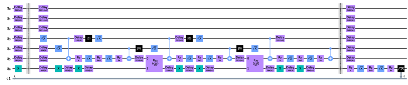
Figure 4: The circuit to apply the channel $\Phi_{(2)}$. Qubit $q_{6}$ on the ibmq_lagos serves as $B$, $q_{5}$ as $A$, and $q_{3}$ and $q_{4}$ as auxiliaries. Figure created using IBM Quantum, generated using Qiskit and the Matplotlib backend. Gates within the two barriers apply $\Phi_{(k)}$, while gates surrounding the barriers are inserted by Qiskit’s channel tomography.

In simulation, one may program the channel $\Phi_{(k)}$ almost exactly. In experiment, there are several challenges. First, IBMQ devices do not natively implement depolarizing channels, since they are typically undesirable in computation. Second, unintended noise on qubit $B$ may induce mixture independently from any process on $A$, confounding intended effects. Third, small, two-qubit rotations also differ from the typical use case of gate-based quantum computers. For the experiment, we apply the following procedure:

1. The device is initialized in the computational basis $\ket{0...0}$ state.

2. Channel tomography preparation gates are applied to qubit $B$.

3. The following sequence of steps is repeated for $k$ rounds:

   1. Apply $\mathcal{E}_{0}$: $S_{Z}$ gates are applied to each of two auxiliary qubits. One $CX$ gate is applied from the first auxiliary to $A$. One Hadamard is applied to $A$. One $CX$ is applied from the second auxiliary to $A$. Reset operations begin on both auxiliaries.

   2. Apply $\Phi_{ZX(\pi/(2k))}$: using the Qiskit class RZXCalibrationBuilder and OpenPulse access, a pulsed implementation of $\Phi_{ZX(\pi/(2k))}$ is applied from qubit $A$ to qubit $B$.

   3. Wait for the next cycle: between each application of $\Phi_{ZX(\pi/(2k))}$ or the beginning or end of the circuit, dynmical decoupling is applied to $B$ via a pair of $X$ gates inserted via Qiskit’s dynamical decoupling routine.

4. $\mathcal{E}$ is applied again without the reset operations.

5. Channel tomography is applied to qubit $B$. Qubit $A$ is assumed to be fully depolarized, as the state of it and the auxiliaries is discarded.

At $k=16$, $|M_{14}|-|M_{23}|<0$, resulting in a negative argument to the logarithms used to solve Equation (12) for $\chi$. This over-rotation in $X$ may result from passive drift, from overrotation in the application of $\Phi_{ZX(\pi/(2k))}$, or even from random fluctuations when both $|M_{14}|$ and $|M_{23}|$ are small. Based on the unexpectedly fast convergence observed in Figure 3.(1) and Figure 3.(3), it appears that a buildup in calibration errors is likely. This explanation is consistent with the difficulty in calibrating $\Phi_{ZX(\pi/(2k))}$ for large values of $k$. Since experiments with $k>15$ may fail to reflect intended parameters, we truncate the results presented in Figure 3 to earlier points.

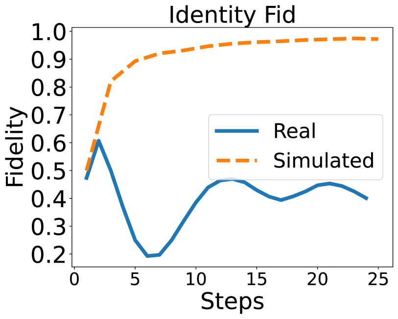
1

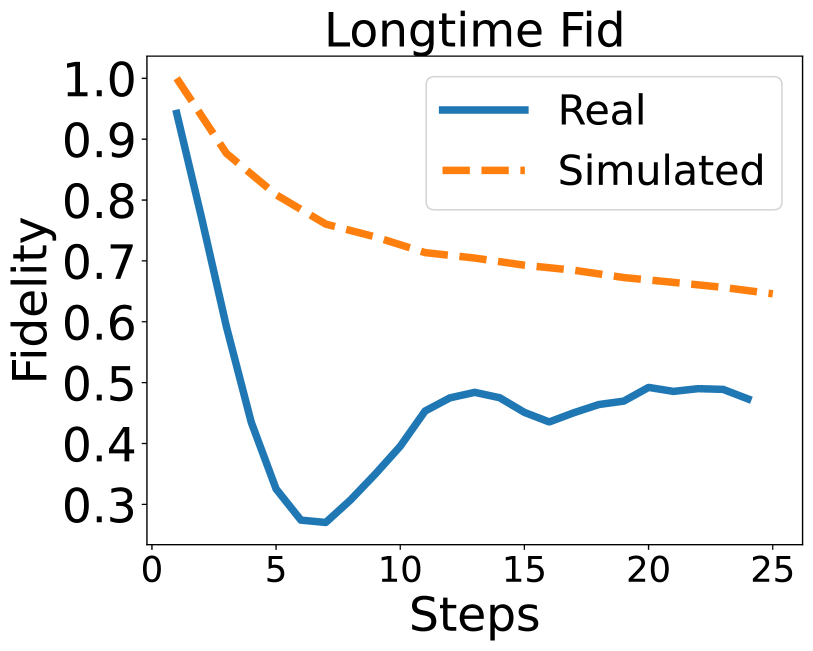
2

Figure 5: Plots of raw metrics for qubit $B$ undergoing the channel described by Equation (10). (1) Fidelity of induced channel’s Choi matrix with the identity process. (2) Fidelity with the long-time fixed point.

Raw metrics are shown in Figure 5. To better represent and understand the actual channels observed, we use a similar method as the $D^{4}$ model in [47]. While the intended decoherence is $X$-basis dephasing as inferred in Subsection IV, unintended decoherence commonly appears as a combination of depolarizing, amplitude damping, dephasing, and coherent phase drift. Unlike in [47], here we study single channels rather than repeated composition of the same channel, so we do not use the “$t$” parameter considered therein. We make the simplifying assumption that noise is applied simultaneously as in a continuous semigroup - this does not constrain the parameter range of the model but resolves the ambiguity due to non-commutativity of amplitude damping with depolarizing noise and $X$-basis decoherence. We add continuous $X$-basis dephasing to the original model. We denote by $\epsilon$ a depolarizing parameter, by $\eta$ a $Z$-basis amplitude damping parameter, by $\delta$ a $Z$-basis dephasing parameter, by $\theta$ a phase drift angle, and by $\chi$ the same $X$-basis dephasing parameter as in Equation (12).

For small values of $k$, there is an initial increase in fidelity of $\Phi_{(k)}$ with the identity channel on $B$ showinn in Figure 5. Nonetheless, fidelity quickly begins to drop. Experimental results then begin to diverge from noiseless simulation. Though the pulse-based $\Phi_{ZX(\pi/(2k))}$ yields improved performance compared with the default mapping to native gates, it does not decline as $1/k$ but enters a regime of diminishing returns (see [55] for details). Furthermore, each application of $\mathcal{E}_{0}$ requires approximately $1\mu s$ waiting for the auxiliary qubits to reset. Based on the reported $T_{1}$ and $T_{2}$ for qubit $B$, one may reasonably estimate that each application of $\mathcal{E}\circ\Phi_{ZX(\pi/(2k))}$ induces on the order of $1-2\%$ infidelity via passive noise. The effects of unintended hardware noise increase with $k$, contrasting the protective scaling of the Zeno effect. For $k>5$, unintended noise appears to dominate. Not only does fidelity of $\Phi_{(k)}$ with the identity channel quickly begin to decrease, but fidelity with the long-time fixed point (in which $B$ is fully dephased in the $X$ basis) also drops quickly.

A channel is fully characterized by its Choi matrix, the result of applying the channel to one half of a maximally entangled pair. The Choi matrix of an identity channel is given by the density matrix of $(\ket{00}+\ket{11})/\sqrt{2}$, a maximally entangled state in which the output and reference mirror each other. To infer noise parameters from a Choi matrix, we solve for specific elements of the Choi matrix under modeled noise in the computational basis. In particular, letting $M_{j,l}$ denote the $j,l$th entry,

$$\begin{split}M_{11}&=\Big{(}\frac{1}{2}-\frac{\epsilon+2\eta+\chi}{4(\epsilon+\eta+\chi)}\Big{)}e^{-(\epsilon+\eta+\chi)}+\frac{\epsilon+2\eta+\chi}{4(\epsilon+\eta+\chi)}\text{, and }\\ M_{44}&=\Big{(}\frac{1}{2}-\frac{\epsilon+\chi}{4(\epsilon+\eta+\chi)}\Big{)}e^{-(\epsilon+\eta+\chi)}+\frac{\epsilon+\chi}{4(\epsilon+\eta+\chi)}\hskip 2.84544pt.\end{split}$$

Because the channel only touches one half of the Bell pair, we may assume that $M_{22}=1/2-M_{11}$ and that $M_{33}=1/2-M_{44}$. For off-diagonal elements,

$$\begin{split}|M_{14}|+|M_{23}|&=\frac{1}{2}e^{-(\eta/2+\epsilon+\delta)}\\ |M_{14}|-|M_{23}|&=\frac{1}{2}e^{-(\eta/2+\epsilon+\delta+\chi)}\hskip 2.84544pt.\end{split}$$ (29)

These 4 matrix elements suffice to fully define the 4 parameters $\epsilon,\eta,\delta$, and $\chi$. In practice, we find simple a simple formula for $\chi$ as in (12), which allows us to extract this parameter immediately. We then use Scipy’s “scipy.optimize.minimize” subroutine to solve for $\epsilon$ and $\eta$, after which we can easily solve for $\delta$ in terms of $|M_{14}|+|M_{23}|$. We find $\theta$ independently as the phase of $M_{14}$. These inferred parameters uniquely determine $M_{11},M_{22},M_{12},M_{14},M_{23},M_{41},M_{32},M_{33}$, and $M_{44}$. In this model, we assume that other elements are zero.

Figure 6 shows unintended noise parameters over time.

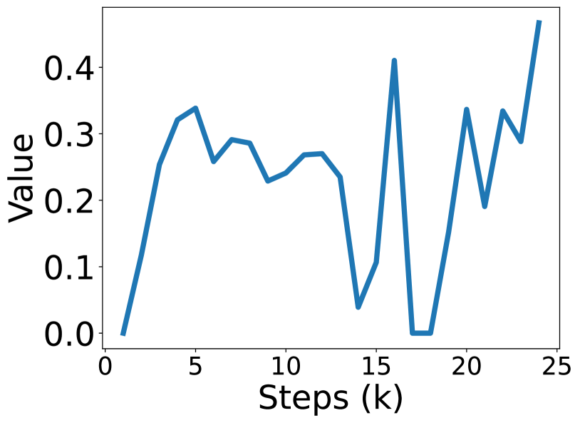
1 $\epsilon$

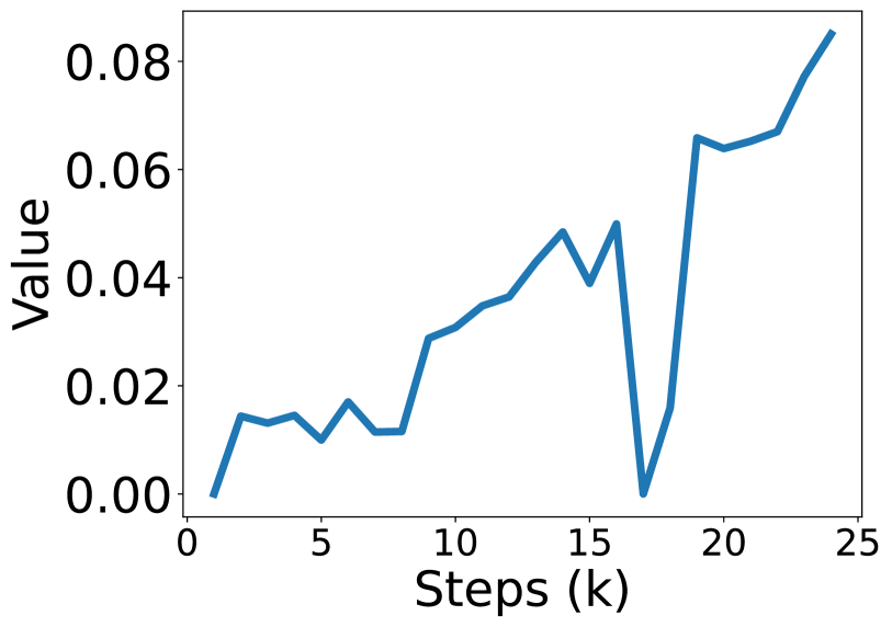
2 $\eta$

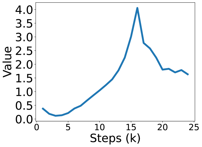
3 $\delta$

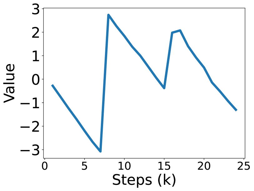
4 $\theta$

Figure 6: Plots of noise parameters by step number.

While coherent phase drift is non-trivial, this should not have a substantial effect on inferred $X$-basis dephasing. Otherwise, the dominant noise contribution is from $Z$-basis dephasing, which by reducing the magnitude of off-diagonal elements may reduce the precision of the inferred $\chi$ in Equation (12). Dominance of $Z$-basis dephasing as unintended noise is consistent with passive decoherence during resets, but this explanation is not consistent with the similarity in reported $T_{1}$ and $T_{2}$ noise and lack of substantial amplitude damping contribution. Dephasing noise appears to peak at 16 steps, the same point where $\chi$ becomes negative (and is set to 0 in further parameter inference), while other parametrs show spikes at this point. This observation is consistent with the explanation that $\chi$ becomes negative due to uncertainty in the ratio of the sum and difference in Equation (29) when both have small values. It also appear that the pulsed interactions might drive dephasing noise or suppress other kinds of noise.

A qubit undergoing dephasing noise in two bases also is effectively depolarized. Though complete depolarization is indistinguishable from complete dephasing in both of two mutually unbiased bases, the partial versions of these channels do allow one to distinguish noise contributions via the ratio of each dephased contribution to the depolarized portion. In Figure 6, the depolarizing parameter corresponds to that left over after accounting for both kinds of dephasing. Here we see evidence that in this case, depolarizing noise arises more as a consequence of dephasing in two bases than via direct replacement of the state by complete mixture.

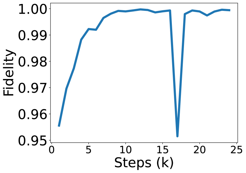
1

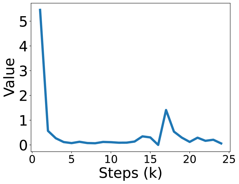
2

Figure 7: (1) Process fidelity of inferred model’s reconstructed channel with the observed channel. (2) Inferred dephasing parameter $\chi$ as in Equation (12).

Finally, we arrive at the culmination of this analysis in Figure 7. First, Figure 7.(1) shows the process fidelity of the inferred model with the channel tomography. Since observed fidelities are at least 95% with a mean of 99%, the noise model does not lose much information about the state. Figure 7.(2) shows the inferred $\chi$ parameter, which is used to reconstruct the cleaned data for Figure 3.

References

- Lindblad [1976] G. Lindblad, Communications in Mathematical Physics 48, 119 (1976).
- Gorini et al. [1976] V. Gorini, A. Kossakowski, and E. C. G. Sudarshan, Journal of Mathematical Physics 17, 821 (1976), publisher: American Institute of Physics.
- Junge et al. [2019] M. Junge, N. LaRacuente, and C. Rouzé, arXiv:1911.08533 [math-ph, physics:quant-ph] (2019).
- Gao et al. [2021] L. Gao, M. Junge, and H. Li, arXiv:2102.04434 [quant-ph] (2021).
- Gao and Rouzé [2021] L. Gao and C. Rouzé, arXiv:2102.04146 [quant-ph] (2021).
- Carlen and Maas [2017] E. A. Carlen and J. Maas, Journal of Functional Analysis 273, 1810 (2017).
- Arnold et al. [1998] A. Arnold, P. Markowich, G. Toscani, and A. Unterreiter, , 77 (1998).
- Bobkov and Tetali [2003] S. Bobkov and P. Tetali, in Proceedings of the thirty-fifth annual ACM symposium on Theory of computing, STOC ’03 (Association for Computing Machinery, New York, NY, USA, 2003) pp. 287–296.
- Kastoryano and Temme [2013] M. J. Kastoryano and K. Temme, Journal of Mathematical Physics 54, 052202 (2013), publisher: American Institute of Physics.
- Bardet et al. [2021] I. Bardet, M. Junge, N. LaRacuente, C. Rouzé, and D. Stilck França, IEEE Transactions on Information Theory , 1 (2021), conference Name: IEEE Transactions on Information Theory.
- Stilck França and García-Patrón [2021] D. Stilck França and R. García-Patrón, Nature Physics 17, 1221 (2021), number: 11 Publisher: Nature Publishing Group.
- Bardet et al. [2022a] I. Bardet, A. Capel, L. Gao, A. Lucia, D. Pérez-García, and C. Rouzé, “Rapid thermalization of spin chain commuting Hamiltonians,” (2022a).
- Hayden and Sorce [2021] P. Hayden and J. Sorce, arXiv:2108.08316 [cond-mat, physics:math-ph, physics:quant-ph] (2021).
- noa [2021] “Solving the Lindblad dynamics of a qubit chain — Qiskit Dynamics Solvers 0.2.1 documentation,” (2021).
- Burgarth et al. [2019] D. Burgarth, P. Facchi, H. Nakazato, S. Pascazio, and K. Yuasa, Quantum 3, 152 (2019), publisher: Verein zur Förderung des Open Access Publizierens in den Quantenwissenschaften.
- Winter [2016] A. Winter, Communications in Mathematical Physics 347, 291 (2016).
- Gao et al. [2020a] L. Gao, M. Junge, and N. LaRacuente, International Journal of Mathematics 31, 2050046 (2020a), publisher: World Scientific Publishing Co.
- Misra and Sudarshan [1977] B. Misra and E. C. G. Sudarshan, Journal of Mathematical Physics 18, 756 (1977), publisher: American Institute of Physics.
- Facchi et al. [2004] P. Facchi, D. A. Lidar, and S. Pascazio, Physical Review A 69, 032314 (2004), publisher: American Physical Society.
- Hahn et al. [2021] A. Hahn, D. Burgarth, and K. Yuasa, arXiv:2112.04242 [quant-ph] (2021).
- Deshpande et al. [2022] A. Deshpande, P. Niroula, O. Shtanko, A. V. Gorshkov, B. Fefferman, and M. J. Gullans, arXiv:2112.00716 [cond-mat, physics:quant-ph] (2022).
- Lloyd [1997] S. Lloyd, Physical Review A 55, 1613 (1997), publisher: American Physical Society.
- Shor [2002] P. W. Shor, (2002), in lecture notes, MSRI Workshop on Quantum Computation.
- Devetak [2005] I. Devetak, IEEE Transactions on Information Theory 51, 44 (2005), conference Name: IEEE Transactions on Information Theory.
- Barreiro et al. [2008] J. T. Barreiro, T.-C. Wei, and P. G. Kwiat, Nature Physics 4, 282 (2008), number: 4 Publisher: Nature Publishing Group.
- Erez et al. [2004] N. Erez, Y. Aharonov, B. Reznik, and L. Vaidman, Physical Review A 69, 062315 (2004), publisher: American Physical Society.
- Pimsner and Popa [1986] M. Pimsner and S. Popa, Annales scientifiques de l’École Normale Supérieure 19, 57 (1986).
- Jones [1983] V. F. R. Jones, Inventiones mathematicae 72, 1 (1983).
- Gross [1975a] L. Gross, American Journal of Mathematics 97, 1061 (1975a), publisher: Johns Hopkins University Press.
- Gross [1975b] L. Gross, Duke Mathematical Journal 42, 383 (1975b), publisher: Duke University Press.
- Bardet and Rouzé [2018] I. Bardet and C. Rouzé, arXiv:1803.05379 [math-ph, physics:quant-ph] (2018).
- Bardet [2017] I. Bardet, arXiv:1710.01039 [math-ph, physics:quant-ph] (2017).
- Gao et al. [2020b] L. Gao, M. Junge, and N. LaRacuente, Annales Henri Poincaré 21, 3409 (2020b).
- Barankai and Zimborás [2018] N. Barankai and Z. Zimborás, arXiv:1811.02509 [math-ph, physics:quant-ph] (2018).
- Möbus and Wolf [2019] T. Möbus and M. M. Wolf, Journal of Mathematical Physics 60, 052201 (2019), publisher: American Institute of Physics.
- Burgarth et al. [2020] D. Burgarth, P. Facchi, H. Nakazato, S. Pascazio, and K. Yuasa, Quantum 4, 289 (2020), publisher: Verein zur Förderung des Open Access Publizierens in den Quantenwissenschaften.
- Becker et al. [2021] S. Becker, N. Datta, and R. Salzmann, Annales Henri Poincaré (2021), 10.1007/s00023-021-01075-8.
- Möbus and Rouzé [2021] T. Möbus and C. Rouzé, arXiv:2111.13911 [math-ph, physics:quant-ph] (2021).
- Kato [1950] T. Kato, Journal of the Physical Society of Japan 5, 435 (1950), publisher: The Physical Society of Japan.
- LaRacuente [2022] N. LaRacuente, Journal of Mathematical Physics 63, 122203 (2022), publisher: American Institute of Physics.
- Bardet et al. [2022b] I. Bardet, A. Capel, and C. Rouzé, Annales Henri Poincaré 23, 101 (2022b).
- Petz [1988] D. Petz, The Quarterly Journal of Mathematics 39, 97 (1988).
- Gao et al. [2022] L. Gao, M. Junge, N. LaRacuente, and H. Li, “Complete order and relative entropy decay rates,” (2022).
- Watrous [2018] J. Watrous, The Theory of Quantum Information (Cambridge University Press, Cambridge, 2018).
- Junge and Xu [2006] M. Junge and Q. Xu, Journal of the American Mathematical Society 20, 385 (2006).
- Junge et al. [2018] M. Junge, R. Renner, D. Sutter, M. M. Wilde, and A. Winter, Annales Henri Poincaré 19, 2955 (2018).
- LaRacuente et al. [2022] N. LaRacuente, K. N. Smith, P. Imany, K. L. Silverman, and F. T. Chong, arXiv:2201.08825 [quant-ph] (2022).
- Umegaki [1962] H. Umegaki, Kodai Mathematical Seminar Reports 14, 59 (1962), publisher: Tokyo Institute of Technology, Department of Mathematics.
- Kosaki [1984] H. Kosaki, Journal of Functional Analysis 56, 29 (1984).
- [50] “sum(a^n/n!, n, m, infinity) - Wolfram|Alpha,” .
- Robbins [1955] H. Robbins, The American Mathematical Monthly 62, 26 (1955), publisher: Mathematical Association of America.
- Suzuki [1976] M. Suzuki, Communications in Mathematical Physics 51, 183 (1976).
- Gao et al. [2018] L. Gao, M. Junge, and N. Laracuente, Journal of Mathematical Physics 59, 062203 (2018), publisher: American Institute of Physics.
- Magesan et al. [2012] E. Magesan, J. M. Gambetta, and J. Emerson, Physical Review A 85, 042311 (2012), publisher: American Physical Society.
- Stenger et al. [2021] J. P. T. Stenger, N. T. Bronn, D. J. Egger, and D. Pekker, Physical Review Research 3, 033171 (2021).