Optical angular momentum in atomic transitions: a paradox

Abstract

Stated simply the paradox is as follows: it is clear that the orbital angular momentum of a light beam in its direction of propagation is an intrinsic quantity, and therefore has the same value everywhere in the beam. How then can a Gaussian beam, with precisely zero orbital angular momentum, drive a (single-photon) quadrupole transition which requires the transfer of angular momentum $2\hbar$ to an absorbing atom?

I Introduction

It has long been appreciated that light has mechanical properties including energy, momentum and also angular momentum. The energy property was known to the ancients but the first suggestion of the momentum appears to be by Kepler who observed that the dust tails of comets point away from the sun and ascribed this effect to radiation pressure Kepler . It was Maxwell who first calculated the radiation pressure due to sunlight on the surface of the earth Maxwell and Poynting who quantified the momentum and energy flux associated with the electromagnetic field Poyntingvec ; Poyntingbook . Poynting also proposed that light can carry angular momentum and suggested, in particular, that angular momentum was associated with circular polarisation Poyntingspin .

The modern study of optical angular momentum, and in particular of orbital angular momentum, can be traced to the work of Allen et al Les who showed that laser modes, specifically the Laguerre-Gaussian modes, carry $\ell\hbar$ units of orbital angular momentum about the beam axis for each photon, where $\ell$ is the charge of the phase vortex at the centre of the mode. Within the paraxial regime we can assign also a separate spin part of $\pm\hbar$ per photon associated with the circular polarisation. The combination of these orbital and spin parts of the optical angular momentum has proven to be most versatile and has found numerous and diverse applications OAMbook ; Bekshaev ; Alison ; Andrews ; PhilTrans .

Optical angular momentum plays a crucial role in the interaction between light and matter. Selection rules between atomic and molecular energy levels are determined in terms of changes in angular momentum Condon ; Kuhn ; CohenT ; Sobelman , as are transitions occurring in nuclei Rose . The strongest transitions in an atom are those mediated by the electric dipole interaction. For these the conservation of angular momentum imposes selection rules on the electronic total angular momentum and on the angular momentum component quantum numbers in the form $\Delta l=\pm 1$ and $\Delta m=0,\pm 1$. (It is an accident of history that the letter $l$ is used both for the $z$-component of the optical angular momentum and also for the electronic total angular momentum quantum number. In the hope of avoiding confusion we use different fonts for these two quantities, $\ell$ for the optical orbital angular momentum and $l$ for the total electronic angular momentum quantum number.) The required angular momentum is readily provided by the absorption of a photon with the appropriate polarisation; in particular the absorption of a left- or right-circularly polarised photon exciting a transition with $\Delta m=+1$ or $-1$ respectively. The absorption of a photon in this way transfers energy to excite the atom and spin angular momentum to change the internal angular momentum. It is not possible for the required angular momentum to be provided by the orbital angular momentum of the field Bennett . The absorbed photon transfers, also, linear momentum and also orbital angular momentum to the centre of mass motion of the atom Lembessis . The last of these has its strongest and most subtle effect when the atom is in the vicinity of an optical vortex BerryDennis ; Qcore ; superkick .

In this paper we are principally concerned with angular momentum transfer to an atom via higher-order multipolar transitions and, in particular, by an electric quadrupole transition, in which the angular momentum of the atom changes by $\Delta l=+2$, $\Delta m=+2$. We have in mind something like the $5^{2}S_{1/2}$ to $5^{2}D_{5/2}$ transition in Rubidium 87 Kien , but our analysis is not restricted to a particular transition or atom. In an elegant experiment, Afanasev et al showed that such a transition can be enhanced if the atom (in the experiment it was a calcium 40 ion) is held at the vortex core of a suitably prepared beam. In one case in particular, a circularly polarised $\ell=1$ beam was employed, so that the required two quanta of angular momentum are provided by one of optical spin angular momentum and one of optical orbital angular momentum Afanasev .

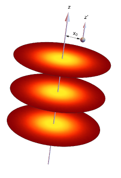
Figure 1: An atom displaced a distance $x_{0}$ from the z-axis of a Gaussian beam. This beam has flat phase fronts and therefore the orbital angular momentum about the beam’s $z$-axis is zero. The orbital angular momentum about the atom’s axis $z^{\prime}$ is also identically zero, as orbital angular momentum is intrinsic, and therefore we must ask from where the atom can obtain the two quanta of angular momenta required to drive the stated quadrupole transition.

The paradox in our title arises when we consider driving the quadrupole transition by a circularly polarised beam of light carrying zero units of orbital angular momentum, as shown in Figure 1. The phase fronts are approximately perpendicular to the propagation direction and do not have the helical form characteristic of the presence of orbital angular momentum Les ; OAMbook ; Bekshaev ; Alison ; Andrews ; PhilTrans . Such a beam carries only one quantum of spin angular momentum per photon and, moreover, as both the spin and the orbital angular momenta are intrinsic, it appears to be the case that whatever the position of the atom, no quanta of orbital angular momenta are available. How then is the angular momentum conserved in such a transition?

II Optical orbital angular momentum: intrinsic or extrinsic?

In mechanics it is often helpful and straightforward to separate spin and orbital angular momentum. The motion of the Earth, for example, is readily separated into an intrinsic spin component (responsible for the cycle of days and nights) and an extrinsic orbital motion associated with the calendar year. The former is intrinsic in that its value does not depend on the position of the chosen axis, but the latter does depend on the choice of axis and so is extrinsic. For light the situation is more subtle. We have long known how to extract spin and orbital parts Darwin but it is clear that, although these are separately measurable, neither is a true angular momentum vanEnk ; Rot ; natures .

We are concerned with the component of the optical angular momentum in the direction of propagation of our light beam. Here we can readily identify separate spin and orbital parts of the total angular momentum and, indeed, observe the individual contributions from these Anna . However in this case both the spin and orbital parts are intrinsic, that is they are unchanged if we evaluate them about any axis parallel to the direction of the beam. Berry provided a simple and general proof of this, which we reproduce here Berry .

The spin part of the optical angular momentum is intrinsic and we can determine the extrinsic or intrinsic nature of the orbital part by examining the total angular momentum. Consider a beam of light propagating in the $z$-direction, carrying some quantity of the $z$-component of angular momentum. If we shift by ${\bf r}_{0}$ the axis about which the angular momentum is evaluated, then we find that the total angular momentum changes to

$$J^{\prime}_{z}=J_{z}-({\bf r}_{0}\times{\bf p})_{z}\,,$$ (1)

where ${\bf p}$ is the total momentum of the beam. Yet if the beam is propagating in the $z$-direction, then the transverse components of the total momentum of the light $p_{x}$ and $p_{y}$, are both zero and we conclude that the angular momentum of the beam is independent of the position about which it is determined: $J^{\prime}_{z}=J_{z}$. The spin angular momentum is intrinsic and it follows, therefore, that the orbital part is also intrinsic.

III Electric dipole and electric quadrupole transitions

To highlight the issue of angular momentum conservation, we present here simple analyses of a $\Delta m=+1$ electric dipole transition and a $\Delta m=+2$ quadrupole transition, both driven by a circularly polarised Gaussian beam of light which carries $\hbar$ units of spin angular momentum per photon, but zero units of orbital angular momentum. For definiteness we consider a pair of transitions from the ground state of atomic Rubidium 87, $5^{2}S_{1/2}$, to the $5^{2}P_{3/2}$ level and to the $4^{2}D_{5/2}$ level. The first of these is an electric dipole transition with $\Delta l=+1$ and $\Delta m=+1$, corresponding to the gain, by the atom, of one quantum $\hbar$ of angular momentum. The second is an electric quadrupole transition in which the atom acquires two quanta, $2\hbar$, of angular momentum from the single photon absorbed.

III.1 Electric dipole transition

The electric dipole transition is associated with the interaction energy of the form Edwin ; Rodney

$$V_{d}=-D_{i}E_{i}\,,$$ (2)

where ${\bf D}$ is the dipole moment operator for the atom and ${\bf E}$ is the resonant driving electric field. Here we adopt the summation convention in which repeated indices imply a summation over the three cartesian coordinates. The dipole moment has the form

$$D_{i}=-e\sum_{\alpha}r^{\alpha}_{i}$$ (3)

where the summation runs over all the atomic charges. For Rubidium we need consider only the valence electron and so replace the summation by the coordinates (relative to the nucleus) of this single electron, so the dipole moment operator becomes

$$D_{i}=-er_{i}\,.$$ (4)

Let us consider the interaction matrix element for the transition from the ground state, $5^{2}S_{1/2}$, to the excited state, $5^{2}P_{3/2}$. As we are increasing the energy of the atom, we can associate this with photon absorption and therefore with the positive frequency, $e^{-i\omega t}$, part of the electric field. We consider a monochromatic paraxial (or weakly focussed) beam of light propagating in the $z$-direction. Hence we can write the transition matrix element from the ground state ($|g\rangle=|5,0,0,1/2\rangle$, where the four entries in this state correspond to the quantum numbers $n$, $l$, $m$ and $s$) to the excited state ($|e\rangle=|5,1,1,1/2\rangle$) in the form

$$\langle e|V_{d}|g\rangle=e\langle e|r_{i}|g\rangle E_{i}({\bf R})e^{-i\omega t}\,.$$ (5)

Here $E_{i}({\bf R})$ is the space-dependent part of the complex electric field at the position of the atom. The dominant components of the electric field lie in the $x-y$ plane and there is no need to consider, for our purposes, the much smaller component in the $z$-direction.

To determine the optimal form of the field with which to drive the transition, we need to evaluate the required form of the dipole matrix element. To this end we note that the wavefunction for the electron to which the field is coupled can be written in the form

$$\psi_{n,l,m}({\bf r})=R_{n,l}Y^{m}_{l}(\vartheta,\varphi)\,,$$ (6)

where $Y^{m}_{l}(\vartheta,\varphi)$ is the spherical harmonic Condon ; Kuhn ; CohenT ; Sobelman and we have omitted mention of the electron spin, which does not change in the transition. We then find that the dipole matrix element is

$$d_{i} =\langle e|D_{i}|g\rangle$$

$$=-e\int_{0}^{\infty}r^{2}dr\int_{0}^{\pi}\sin\vartheta\int_{0}^{2\pi}d\varphi R_{5,1}(r)Y^{1*}_{1}(\vartheta,\varphi)r_{i}R_{5,0}(r)Y^{0}_{0}(\vartheta,\varphi)\,,$$ (7)

where the spherical harmonics are

$$Y^{0}_{0}(\vartheta,\varphi) =\frac{1}{2}\sqrt{\frac{1}{\pi}}$$

$$Y^{1}_{1}(\vartheta,\varphi) =-\sqrt{\frac{3}{8\pi}}\sin\vartheta e^{i\varphi}\,.$$ (8)

It follows that the components of the dipole matrix element are

$$d_{x} =\frac{e}{\sqrt{6}}\int_{0}^{\infty}r^{2}drR_{5,1}rR_{5,0}=d$$

$$d_{y} =-id\,.$$ (9)

Hence the matrix element of the interaction energy is

$$\langle e|V_{d}|g\rangle=-d(E_{x}({\bf R})-iE_{y}({\bf R}))e^{-i\omega t}\,.$$ (10)

To maximise the magnitude of this, and thereby find the maximum rate for driving this transition, we simply set $E_{y}=iE_{x}$, so that the electric field takes the form

$${\bf E}({\bf R})=\frac{E_{0}({\bf R})}{\sqrt{2}}(\hat{\bf x}+i\hat{\bf y})e^{-i\omega t}\,,$$ (11)

where $\hat{\bf x}$ and $\hat{\bf y}$ are unit vectors in the $x$- and $y$-directions. Note that this corresponds to a field with left-handed circular polarisation, corresponding to $+\hbar$ spin angular momentum per photon.

Whatever the position of the absorbing atom, the intrinsic spin angular momentum of the light provides the required single quantum of angular momentum about the displaced $z$-axis centred on the position of the atom. The only dependence on position comes from the spatial variation of the strength of the field $E_{0}$ and hence the intensity.

III.2 Electric quadrupole excitation

The electric quadrupole interaction energy depends on the derivatives of the electric field at the position of the atom:

$$V_{q}=Q_{ij}\nabla_{i}E_{j}\,,$$ (12)

where $Q_{ij}$ is the quadrupole moment defined to be Edwin ; Rodney

$$Q_{ij}=-\frac{1}{2}r_{i}r_{j}\,.$$ (13)

Note that both the electric dipole and electric quadrupole interactions can readily be derived within the Power-Zienau-Woolley multipolar expansion Bennett ; Edwin . We are interested in transitions in our Rubidium atom from the ground state, $5^{2}P_{1/2}$, to the excited state, $4^{2}D_{5/2}$. We can write the transition matrix element from the ground to the excited state ($|e\rangle=|4,2,2,1/2\rangle$) in the form

$$\langle e|V_{q}|\rangle=-\frac{1}{2}\langle e|r_{i}r_{j}|g\rangle\nabla_{j}E_{i}e^{-i\omega t}\,,$$ (14)

where the derivatives of the field are evaluated at the position of the atom ${\bf R}$.

To determine the form of the field required to drive this transition, we need to evaluate the quadrupole matrix element. In order to calculate this we require the spherical harmonic associated with the excited state:

$$Y^{2}_{2}(\vartheta,\varphi)=\frac{1}{4}\sqrt{\frac{15}{2\pi}}\sin^{2}\vartheta e^{i2\varphi}\,.$$ (15)

Hence our quadrupole matrix elements $\langle e|Q_{ij}|g\rangle$ are

$$q_{xx} =\langle e|Q_{xx}|g\rangle$$

$$=-\frac{e}{2}\frac{1}{\sqrt{30}}\int_{0}^{\infty}r^{2}drR_{4,2}(r)r^{2}R_{5,0}(r)$$

$$=\mathcal{Q}$$

$$q_{xy} =-i\mathcal{Q}=q_{yx}$$

$$q_{yy} =-\mathcal{Q}\,.$$ (16)

To proceed let us consider the possible forms for the driving field. As noted above, the dominant components will be in the $x$- and $y$-directions and it is the derivatives of the field that couple to the atom. To this end we expand the components of the electric field as a Taylor-Maclaurin series in the form

$$E_{x}({\bf r}) =E_{x}({\bf R})e^{-i\omega t}+(x-X)\frac{\partial}{\partial x}E_{x}({\bf R})e^{-i\omega t}+(y-Y)\frac{\partial}{\partial y}E_{x}({\bf R})e^{-i\omega t}+\cdots$$

$$=E_{x}({\bf R})e^{-i\omega t}+[\alpha(x-X)+\beta(y-Y)]E^{(1)}({\bf R})e^{-i\omega t}+\cdots$$

$$E_{y}({\bf r}) =E_{y}({\bf R})e^{-i\omega t}+(x-X)\frac{\partial}{\partial x}E_{y}({\bf R})e^{-i\omega t}+(y-Y)\frac{\partial}{\partial y}E_{y}({\bf R})e^{-i\omega t}+\cdots$$

$$=E_{y}({\bf R})e^{-i\omega t}+[\gamma(x-X)+\delta(y-Y)]E^{(1)}({\bf R})e^{-i\omega t}+\cdots\,.$$ (17)

Without loss of generality, we can fix select our four complex constants such that $|\alpha|^{2}+|\beta|^{2}+|\gamma|^{2}+|\delta|^{2}=2$. With this choice we fix $E^{(1)}({\bf R})$ to be

$$E^{(1)}({\bf R})=\left.\frac{1}{\sqrt{2}}\left[\sum_{i,j=x,y}\left(\nabla_{i}E_{j}\right)\left(\nabla_{i}E^{*}_{j}\right)\right]^{1/2}\right|_{\bf R}\,.$$ (18)

We can compare this with the required form for our particular transition, for which we have calculated the quadrupole matrix elements, Eq. (III.2). Thus,

$$Q_{ij}\nabla_{i}E_{j}=E^{(1)}e^{-i\omega t}\mathcal{Q}(\alpha-i\beta-i\gamma-\delta)\,.$$ (19)

Clearly this is maximised if the magnitudes of each of our parameters $\alpha,\beta,\gamma$ and $\delta$ are equal. There is one arbitrary phase, but if we choose $\alpha$ to be real and positive, then the strongest driving occurs for

$$\alpha=\frac{1}{\sqrt{2}}\,,\quad\beta=\frac{i}{\sqrt{2}}=\gamma\,,\quad\delta=-\frac{1}{\sqrt{2}}\,.$$ (20)

Note that the fact that $\delta=-\alpha$ is a consequence of the transversality of the electric field $(\nabla_{i}E_{i}=0)$. The values of $\alpha,\beta,\gamma$ and $\delta$ correspond to an electric field in the vicinity of the atom of the form

$${\bf E}({\bf r})={\bf E}({\bf R})e^{-i\omega t}+E^{(1)}e^{-i\omega t}[(x-X)+i(y-Y)]\frac{1}{\sqrt{2}}(\hat{\bf x}+i\hat{\bf y})\,,$$ (21)

the second term of which corresponds to a circularly polarised $\ell=+1$ beam, with a charge $+1$ phase vortex centred on the atom, at $(X,Y)$, corresponding to $+\hbar$ of orbital angular momentum per photon.

IV The paradox

We have determined the required form of the electric field in order to drive our quadrupole transition; it should be circularly polarised, with an $\ell=+1$ phase vortex centred on the position of the atom. Let us see how a simple circularly polarised Gaussian beam performs. To this end consider an electric field of the form

$${\bf E}=E_{0}\frac{1}{\sqrt{2}}(\hat{\bf x}+i\hat{\bf y})\frac{1}{\sqrt{\pi}w_{0}}\exp\left(-\frac{(x^{2}+y^{2})}{2w_{0}^{2}}\right)e^{-i\omega t}\ .$$ (22)

It is straightforward to calculate the quadrupole coupling matrix element for an atom at position $(X,Y)$ in this field:

$$\langle e|V_{q}|g\rangle=E_{0}\mathcal{Q}\sqrt{\frac{2}{\pi}}\frac{1}{w^{3}_{0}}(X+iY)\exp\left(-\frac{(X^{2}+Y^{2})}{2w^{2}_{0}}\right)\,.$$ (23)

This is non-zero everywhere apart from along the $z$-axis, corresponding to the centre of the beam, for which $X=0=Y$. The perturbative transition probability, which is proportional to the squared modulus of this matrix element, is greatest for an atom at a distance $w_{0}$ from the centre of the beam, where the gradient of the magnitude of the field is greatest.

It follows that a circularly polarised Gaussian beam with only one quantum of angular momentum per photon can readily excite a quadrupole transition requiring two quanta of angular momentum. Moreover, because the orbital angular momentum is an intrinsic quantity, the orbital angular momentum of the beam about an axis passing through the atom is also zero. The puzzle, therefore, is where can the required second quantum of angular momentum have come from?

V An insight from quantum theory

We recall that a mode of well-defined orbital angular momentum is an eigenmode of the differential operator $-i\partial/\partial\phi$. Indeed it was the similarity between this property and the form of the quantum mechanical operator for the $z$-component of the angular momentum $L_{z}=-i\hbar\partial/\partial\phi$ that led to the conclusion that such eigenmodes carry $\ell\hbar$ of orbital angular momentum for each photon Les . The $z$-component of the orbital angular momentum about an axis shifted from the $z$-axis to $x=x_{0}$, $L^{\prime}_{z}$ is related to that about the $z$-axis $L_{z}$ by

$$L^{\prime}_{z}=L_{z}-x_{0}p_{y}\,,$$ (24)

where $p_{y}$ is the operator corresponding to the $y$-component of the linear momentum. As in Berry’s demonstration, this means that the total values of $L_{z}$ and $L^{\prime}_{z}$, which correspond to the expectation values in quantum theory, are the same Berry . The operators $L_{z}$ and $L^{\prime}_{z}$, however, are incompatible in that they do not commute:

$$[L^{\prime}_{z},L_{z}]=i\hbar x_{0}p_{x}$$ (25)

and it follows that $L_{z}$ and $L^{\prime}_{z}$ do not share common eigenmodes. Hence an eigenmode of $\hat{L}_{z}$ must correspond to a superpositon of eigenmodes of $L^{\prime}_{z}$. It is worth remarking that this simple idea does not seem to appear in texts concerned with the quantum theory of angular momentum RoseAM ; Brink ; Edmonds ; BiedenharnEd ; BiedenharnBook ; Zare . We note, however, that the angular momenta about different axes have been shown to occur for free electrons moving in a uniform magnetic field making it possible to separate angular momenta associated with the cyclotron and diamagnetic angular momenta Greenshields . It is worth noting that in the commutator (25), $x_{0}$ can be arbitrarily large. This is a reflection of the fact that the difference between $L_{z}$ and $L^{\prime}_{z}$ is the product of the $y$-component of the momentum operator and $x_{0}$, the distance between the two rotation axes considered. This is reminiscent of the parallel axes theorem in mechanics Kibble .

Consider a normalised wavefunction of the same form as our Gaussian mode:

$$\psi(x,y)=\frac{1}{\sqrt{\pi}w_{0}}\exp\left(-\frac{(x^{2}+y^{2})}{2w^{2}_{0}}\right)\,.$$ (26)

This is an eigenfunction of $L_{z}$ with eigenvalue $0$ and therefore the expectation value of $L^{\prime}_{z}$ is also $0$. It is not an eigenfunction of $L^{\prime}_{z}$, however, and has the non-zero variance

$$\Delta L^{\prime 2}_{z}=x^{2}_{0}\langle p^{2}_{y}\rangle=\frac{\hbar^{2}x^{2}_{0}}{2w^{2}_{0}}\,.$$ (27)

When expressed in terms of the corresponding orbital angular momentum numbers $\ell$ and $\ell^{\prime}$ (associated with the operators $L_{z}$ and $L^{\prime}_{z}$ respectively) this variance becomes

$$\Delta\ell^{\prime 2}=\frac{x^{2}_{0}}{2w^{2}_{0}}\,.$$ (28)

This indicates that our mode with zero orbital angular momentum about the $z$-axis includes a superposition of a range of eigenmodes of the orbital angular momentum about our displaced axis and suggests that our atom, undergoing a quadrupole transition, absorbs a photon from the $\ell^{\prime}=+1$ eigenmodes of $L^{\prime}_{z}$ within this superposition.

To test the idea suggested above we seek to expand our Gaussian mode in terms of a complete set of angular-momentum eigenmodes centred on the position of the atom. We introduce a primed set of coordinates, $(x^{\prime},y^{\prime})$ or $(\rho^{\prime},\phi^{\prime})$, centred on the position of the atom. In terms of these coordinates our normalised Gaussian mode has the form

$$\psi(x^{\prime},y^{\prime})=\frac{1}{\sqrt{\pi}w_{0}}\exp\left(-\frac{[(x^{\prime}+x_{0})^{2}+y^{\prime 2}]}{2w^{2}_{0}}\right)\,.$$ (29)

The Laguerre-Gaussian modes are all eigenmodes of $L^{\prime}_{z}$ angular momentum and we can use them as a complete basis Siegman ; Milonni :

$$u_{p^{\prime}\ell^{\prime}}(\rho^{\prime},\phi^{\prime})=\frac{1}{w_{0}}\left(\frac{p^{\prime}!}{\pi(|\ell^{\prime}|+p^{\prime})!}\right)^{1/2}\exp\left(-\frac{\rho^{\prime 2}}{2w^{2}_{0}}\right)\left(\frac{\rho^{\prime}}{w_{0}}\right)^{|\ell^{\prime}|}L^{|\ell^{\prime}|}_{p^{\prime}}\left(\frac{\rho^{\prime 2}}{w^{2}_{0}}\right)e^{i\ell^{\prime}\phi^{\prime}}\,.$$ (30)

Our expansion has the form

$$\psi(x^{\prime},y^{\prime})=\sum_{\ell^{\prime}=-\infty}^{\infty}\sum_{p^{\prime}=0}^{\infty}c_{p^{\prime}\ell^{\prime}}u_{p^{\prime}\ell^{\prime}}(\rho^{\prime},\phi^{\prime})$$ (31)

and we can exploit the orthonormality of the Laguerre-Gaussian modes to show that the expansion coefficients have the form RobertaRes :

$$c_{p^{\prime}\ell^{\prime}}=(-1)^{p^{\prime}}\left(\frac{1}{(|\ell^{\prime}|+p^{\prime})!p^{\prime}!}\right)^{1/2}\left(-\frac{x_{0}}{2w_{0}}\right)^{2p^{\prime}+|\ell^{\prime}|}\exp\left(-\frac{x^{2}_{0}}{4w^{2}_{0}}\right)\,.$$ (32)

It is clear, in particular, that modes with $\ell^{\prime}=+1$ are present in the superposition. It is from these modes that the atom can absorb a single photon, acquiring in the process $+\hbar$ from the orbital angular momentum to add to the single quantum of spin angular momentum.

We can use the expansion to determine the fraction of the total intensity that is in modes with the required optical angular momentum to drive the quadrupole transition. It is convenient to express this in terms of the probability that any single photon in the beam has orbital angular momentum $\hbar$:

$$P(\ell^{\prime}) =\sum_{p^{\prime}=0}^{\infty}|c_{p^{\prime}\ell^{\prime}}|^{2}$$

$$=\exp\left(-\frac{x^{2}_{0}}{2w^{2}_{0}}\right)I_{\ell^{\prime}}\left(\frac{x^{2}_{0}}{2w^{2}_{0}}\right)\,,$$ (33)

where $I_{n}$ is the modified Bessel function of the first kind of order $n$. It is clear that the mean value of $\ell^{\prime}$ is zero. This follows directly from the fact that $I_{-n}=I_{n}$. We can show by direct calculation from this probability distribution, moreover, that

$$\Delta\ell^{\prime 2}=\frac{x^{2}_{0}}{2w^{2}_{0}}\,,$$ (34)

as anticipated above.

The fraction of the light that is in the correct mode for driving our quadrupole transition is $\exp(-x^{2}_{0}/2w^{2}_{0})I_{1}(x^{2}_{0}/2w^{2}_{0})$. This probability is depicted in Figure 2. We note that if the atom is positioned on the beam axis, so that $x_{0}=0$, this probability is zero and the field cannot drive the quadrupole transition. As we move the position of the atom away from the beam axis the probability that the local orbital angular momentum is $+\hbar$ increases and with it the probability of exciting the transition. At large distances from the beam axis the spread in the distribution of the orbital angular momentum increases and with this the components of the field having $\ell=+1$ decrease in amplitude.

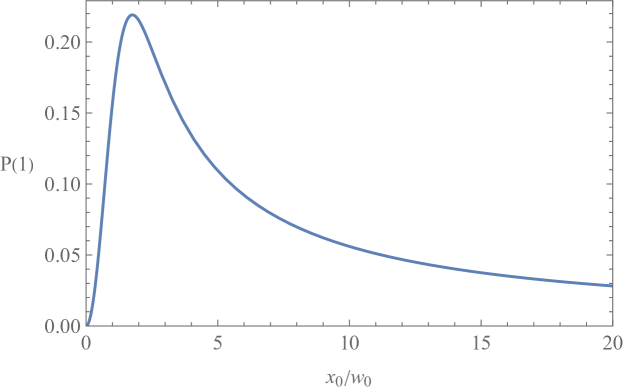
Figure 2: The probability $P(1)$ that any single photon in the beam has orbital angular momentum $\hbar$, as a function of relative position from the beam waist $\frac{x_{0}}{w_{0}}$, as given by Eq. V.

VI Resolution: orbital angular momentum is quasi-intrinsic

It is certainly true that the optical orbital angular momentum is an intrinsic quantity in that the total orbital angular momentum is unchanged by a parallel displacement of the axis about which it is calculated. Yet this is not the whole story as such a displacement leaves the total mean orbital angular momentum unchanged, but the mode is not an eigenmode of the orbital angular momentum about the displaced axis. In this sense it is, perhaps, better to think of the optical orbital angular momentum as a quasi-intrinsic quantity RobertaPRL : it is, in effect, intrinsic on average.

An atom positioned off the axis of a circularly polarised Gaussian beam can interact with any of a superposition of eigenmodes of $L^{\prime}_{z}$ (about an axis passing through the atom). This means that the orbital angular momentum required to conserve angular momentum in a quadrupole transition is readily available to the atom at every position except on the beam axis.

VII Absorption from a beam with no angular momentum

As a final point we ask how our quadrupole transition can be driven by a Gaussian beam that is linearly polarised. The issue here is that such a beam carries zero orbital angular momentum, but also zero spin angular momentum. We have seen that an atom that is not on the beam axis sees a field that is a superposition of orbital angular momentum modes about an axis passing through the atom and, in this way, the field can provide the required quantum of orbital angular momentum.

If the field is linearly polarised then it carries zero units of spin angular momentum. As the spin angular momentum is intrinsic, it is zero at every point in a linearly polarised beam and we can ask where the required quantum of spin angular momentum comes from. The solution to this question mirrors that for the orbital angular momentum paradox in that a linearly polarised beam is an equally weighted superposition of left- and right-handed circularly polarised beams. This follows simply from the decomposition

$$\hat{\bf x}=\frac{1}{\sqrt{2}}\left[\frac{1}{\sqrt{2}}\left(\hat{\bf x}+i\hat{\bf y}\right)+\frac{1}{\sqrt{2}}\left(\hat{\bf x}-i\hat{\bf y}\right)\right]\,.$$ (35)

It follows that half of the light in a linearly polarised beam carries the required spin angular momentum to drive either a $\Delta m=+1$ electric dipole transition or, in combination with the correct component orbital angular momentum mode, a $\Delta m=+2$ electric quadrupole transition.

VIII Conclusion

The orbital angular momentum of a light beam in the direction of propagation is intrinsic, which means that its value is the same everywhere in the beam Berry . Our paradox was that given this intrinsic nature, where does the required angular momentum come from to drive a $\Delta m=+2$ electric quadrupole transition? The resolution, inspired by quantum theory, is that modes of well-defined orbital angular momentum about the beam axis do not also have well-defined orbital angular momentum about a displaced axis; the orbital angular momenta about the $z$- and $z^{\prime}$-axes are, in effect, incompatible quantities.

It follows that a Gaussian beam with precisely zero orbital angular momentum per photon about the beam axis is also a superposition of modes with all possible orbital angular momenta about any axis parallel to that of the beam RobertaRes ; RobertaPRL . The orbital angular momentum required to drive an electric quadrupole transition derives from the modes in this superposition that have $+\hbar$ orbital angular momentum about an axis passing through the atom. This exists at all positions in the beam except on the beam axis.

The ideas and the paradox presented and resolved here apply, also, to higher order multipolar transitions. An electric octopole transition, with $\Delta m=+3$ for example Roberts , can be driven by a circularly polarised Gaussian beam if the absorbing atom is away from the beam axis. In this case there are two quanta of orbital angular momentum required and these will come from those modes in the superposition with $\ell^{\prime}=+2$.

References

References

- (1) Kepler J 1619 De cometis libelli tres (Augustae Vindelicorum: A. Apergeri)
- (2) Maxwell J C 1998 A treatise on electricity and magnetism vol. 2 (Oxford: Oxford University Press) Art. 793
- (3) Poynting J H 1884 On the transfer of energy in the electromagnetic field Phil. Trans. 175 343–361
- (4) Poynting J H 1910 The pressure of light (London: Richard Clay and Sons)
- (5) Poynting J H 1909 The wave-motion of a revolving shaft, and a suggestion as to the angular momentum in a beam of circularly polarised light Proc. Roy. Soc. A 82 560–567
- (6) Allen L, Beijersbergen M W, Spreeuw R J C and Woerdman J P (1992) Orbital angular momentum of light and the transformation of Laguerre-Gaussian laser modes Phys Rev A 45 8185–8189
- (7) Allen L, Barnett S M and Padgett M J 2003 Optical angular momentum (London: Institute of Physics Publishing)
- (8) Bekhshaev A, Soskin M and Vasnetsov M 2008 Paraxial light beams with orbital angular momentum (New York: Nova)
- (9) Yao A M and Padgett M J 2011 Orbital angular momentum: origins, behavior and applications Adv. Opt. Photon. 3 161–204
- (10) Andrews D L and Babiker M eds. 2012 The angular momentum of light (Cambridge: Cambridge University Press)
- (11) Barnett S M, Babiker M and Padgett M J eds. 2017 Optical orbital angular momentum Phil. Trans. R. Soc. 375 issue 2087
- (12) Condon E U and Shortley G H 1953 The theory of atomic spectra (Cambridge: Cambridge University Press)
- (13) Kuhn H G 1962 Atomic spectra (Bristol: Arrowsmith)
- (14) Cohen-Tannoudji C, Diu B and Laloë F Quantum mechanics vol. 2 (New York: Wiley)
- (15) Sobelman I I 1979 Atomic spectra and radiative transitions (Berlin: Springer-Verlag)
- (16) Rose M E 1955 Multipole fields (New York: Wiley)
- (17) Babiker M, Bennett C R, Andrews D L and Dávila Romero L C 2002 Orbital angular momentum exchange in the interaction of twisted light with molecules Phys. Rev. Lett. 89 143601
- (18) Babiker M, Andrews D L and Lembessis V E 2019 Atoms in complex twisted light J. Opt. 21 013001
- (19) Berry M V and Dennis M R 2004 Quantum cores of optical phase singularities J. Opt. A: Pure Appl. Opt. 6 S178–180
- (20) Barnett S M 2008 On the quantum core of an optical vortex J. Mod. Opt. 55 2279–2292
- (21) Barnett S M and Berry M V 2013 Superweak momentum transfer near optical vortices J. Opt. 15 125701
- (22) Kien F L, Ray T, Nieddu T, Busch T and Chormaic S N 2018 Enhancement of the quadrupole interaction fo an atom with the guided light of an ultrathin optical fiber Phys. Rev. A 97 013821
- (23) Afanasev A, Carlson C E, Schmiegelov T, Schultz J, Scmidt-Kaler F ad Solyanik M 2018 Experimental verification of position-dependent angular-momentum selection rules for absorption of twisted light by a bound electron New J. Phys. 20 023032
- (24) Darwin C G 1931 Notes on the theory of radiation Proc. R. Soc. Lond. A 136 36–52
- (25) van Enk S J and Nienhuis G 1994 Spin and orbital angular momentum of photons Europhys. Lett. 25 497–501
- (26) Barnett S M 2010 Rotation of electromagnetic fields and the nature of optical angular momentum J. Mod. Opt. 57 1339–1343
- (27) Barnett S M, Allen L, Cameron R P, Gilson C R, Padgett M J, Speirits F C and Yao A M 2016 On the natures of the spin and orbital parts of optical angular momentum J. Opt. 18 064004
- (28) O’Neil A T, MacVicar I, Allen L and Padgett M J 2002 Intrinsic and extrinsic nature of the orbital angular momentum of light Phys. Rev. Lett. 88 1–4
- (29) Berry M V 1998 Paraxial beams of spinning light in Singular optics eds. Soskin M S and Vasnetsov M V SPIE 3487 6–11
- (30) Power E A 1964 Introductory quantum electrodynamics (London: Longmans)
- (31) Loudon R 2000 The quantum theory of light 3rd ed. (Oxford: Oxford University Press)
- (32) Rose M E 1995 Elementary theory of angular momentum (New York: Dover)
- (33) Brink D M and Satchler G R 1968 Angular momentum 2nd ed. (Oxford: Oxford University Press)
- (34) Edmonds A R 1974 Angular momentum in quantum mechanics (Princeton University Press: Princeton NJ)
- (35) Biedenharn L C and van Dam H eds. 1965 Quantum theory of angular momentum (New York: Academic Press)
- (36) Biedenharn L C and Louck J D 1985 Angular momentum in quantum physics (Cambridge: Cambridge University Press)
- (37) Zare R N 1988 Angular momentum: understanding spatial effects in chemistry and physics (New York: Wiley)
- (38) Greenshields C R, Franke-Arnold S and Stamps R L 2015 Parallel axis theorem for free-space electron wavefunctions New J. Phys. 17 093015
- (39) Kibble T W B 1973 Classical mechanics 2nd ed. (London: McGraw-Hill)
- (40) Siegman A E 1986 Lasers (Sausalito CA: University Science Books)
- (41) Milonni P W and Eberly J H 2010 Laser Physics (Hoboken NJ: Wiley)
- (42) Barnett S M and Zambrini R 2006 Resolution in rotation measurements J. Mod. Opt. 53 613–625
- (43) Zambrini R and Barnett S M 2006 Quasi-intrinsic angular momentum and the measurement of its spectrum Phys. Rev. Lett. 96 113901
- (44) Roberts M, Taylor P, Barwood G P, Gill P, Klein H A and Rowley W R C 1997 Observation of an electric octopole transition in a single ion Phys. Rev. Lett 78 1876