1em \setkomafontcaptionlabel \setkomafontcaption
Global Constraints on Yukawa Operators in the Standard Model Effective Theory
Abstract
CP-violating contributions to Higgs–fermion couplings are absent in the standard model of particle physics (SM), but are motivated by models of electroweak baryogenesis. Here, we employ the framework of the SM effective theory (SMEFT) to parameterise deviations from SM Yukawa couplings. We present the leading contributions of the relevant operators to the fermionic electric dipole moments (EDMs). We obtain constraints on the SMEFT Wilson coefficients from the combination of LHC data and experimental bounds on the electron, neutron, and mercury EDMs, and for the first time, we perform a combined fit to LHC and EDM data allowing the presence of CP-violating contributions from several fermion species simultaneously. Among other results, we find non-trivial correlations between EDM and LHC constraints even in the multi-parameter scans, for instance, when floating the CP-even and CP-odd couplings to all third-generation fermions.
1 Introduction
Charge-Parity (CP) violating contributions to Higgs–fermion couplings are a well-motivated possibility of physics beyond the standard model (SM) that might help address the problem of baryogenesis with new dynamics at the electroweak scale. As is well known, any such contributions are strongly constrained by null measurements of electric dipole moments (EDMs), and less strongly by Higgs production and decay data from colliders. It is also well known that the presence of several CP-violating phases can lead to cancellations and thus weaker bounds [1]. The interplay of EDM and collider constraints, in the presence of several CP-violating Higgs couplings to fermions simultaneously, is less well-known. In Ref. [2] constraints in the presence of two CP-violating parameters have been studied in detail. In this work, we scan over up to six different parameters.
Frequently, model-independent bounds on such interactions have obtained in the so-called “ framework” by rescaling the SM Yukawa coupling by an overall factor and a complex phase. In Ref. [3], bounds on these factors have been obtained by studying contributions to EDMs through Barr–Zee diagrams with internal fermion loops. In Refs. [4, 5] it was shown by explicit calculation within the framework that bosonic two-loop diagrams have a large impact on the EDM bounds for light quarks. However, it was later pointed out that the way these bosonic contributions had been been computed lead to a gauge dependent result [6]. This is related to the fact the naive implementation of the framework, in which only the dimension-four Higgs couplings are modified, is not a consistent quantum field theory. A consistent alternative that resembles the framework most closely would be to use Higgs effective theory (HEFT) [7]. In HEFT, the dimension-four couplings are complemented by the necessary higher dimension interactions to facilitate gauge-independent results.
Another consistent way of obtaining model-independent bounds for CP-violating Higgs-fermion interactions is the use of the SM effective field theory (SMEFT) [8]; see Refs. [2, 9, 10, 11] for recent work in this direction. We take the same approach in this article.
For the purpose of this work, we assume that the contributions to the EDMs of the SM fermions arise from physics at a scale that is sufficiently higher than the electroweak scale. This permits us to parameterize deviations from the SM in terms of operators in SMEFT. We will assume that any of the operator of the form may have non-zero coefficients. Here, is the complex Higgs doublet field, a left-handed doublet fermion field, a right-handed singlet fermion field, and we have suppressed flavour indices. The reason for focussing on this class of operators is that they are the only dimension-six operators that induce tree-level modifications to Higgs–fermion couplings. See Sec. 2 for a detailed discussion. These operators will contribute to leptonic and hadronic dipole moments via a series of matching and renormalization-group (RG) evolution. Our analysis takes into account the leading effects that arise at two-loop order in the electroweak interactions, as well as leading-logarithmic QCD corrections below the electroweak scale. We neglect any effects of CP-odd, flavour off-diagonal operators. The study of these effects is relegated to future work.
To understand the complex interplay between the operators we consider requires us to vary multiple Wilson coefficients simultaneously. To explore this computationally challenging multidimensional parameter space, we make use of the GAMBIT [12] global fitting framework, to which we have added a new module that allows for calculations of EDMs in this EFT, as well as the corresponding experimental likelihoods. We have also expanded the existing ColliderBit [13] module to be able to determine constraints on the Wilson coefficients from measured properties of the Higgs boson at the LHC.
This work contains several new aspects and presents nontrivial results. For the first time, we perform a multi-parameter fit to both LHC and EDM data. This corresponds to a more realistic scenario than single-parameter fits, as in a UV-complete model several CP phases are expected to be present. Moreover, we complement and correct some of the analytic expressions in the literature. In addition to updating existing constraints on either individual CP-odd Yukawa couplings (Figs. 4 and 5), or two CP-odd Yukawa couplings as in Ref. [2] (Fig. 6), we scan over up to six CP-even / CP-odd Yukawa couplings simultaneously for the first time (Figs. 7 - 11). While this represents still only a subset of all Yukawa operators, we argue that with current experimental results, including more parameters will not lead to additional significant constraints. For instance, allowing for any CP-odd contribution to the Yukawa of a light fermion (electron, or up and down quark) would allow to fully cancel the corresponding EDM constraint, thus leaving only the LHC bounds in a trivial way. However, we find several nontrivial effects. Focusing on the heavier fermions, we find an intricate interplay between LHC and precision constraints that weakens the EDM bounds without lifting them fully. Not even by allowing for six independent parameters can we cancel all EDM constraints among the third-generation fermions, and nontrivial EDM bounds remain. A detailed discussion of these issues is found in Sec. 7.
In our analysis, we do not take into account perturbative and hadronic uncertainties. The effects of hadronic uncertainties on EDM bounds have been studied in detail in Ref. [2] (see also Ref. [14]), and will not be repeated here. They are relevant mainly for bounds on CP-violating Higgs couplings to the light quarks that arise from hadronic EDMs, as collider bounds are nearly absent. When allowing for the presence of several Wilson coefficients at the same time, EDM bounds tend to get canceled and only collider bounds remain, so hadronic uncertainties are less relevant. Note also that bounds from arising from the electron EDM have no hadronic uncertainty. However, there is a large, previously overlooked perturbative uncertainty regarding the bottom and charm couplings, as discussed in Sec. 3. This uncertainty is analogous to the case discussed in Ref. [15], and will be studied in detail in a forthcoming publication [16]. As not all relevant higher-order corrections are currently known, they are neglected in this analysis.
This paper is organised as follows. In Section 2 we specify the operators that we want to constrain; namely, those that modify the SM Yukawa couplings at tree level. We then derive the modified Higgs–fermion couplings in the broken electroweak phase. In Sec. 3 we discuss the effective theory valid below the electroweak scale. The analytic contributions of the SMEFT operators to the partonic EDM of leptons and quarks are collected in Sec. 4. Most of these results are taken from the literature, although a few results are presented here for the first time. Furthermore, we correct several errors in the literature. In Sec. 5 we summarize the contributions of the partonic EDMs to the EDM of the physical systems that are actually constrained by experiment. Sec. 6 describes the collider constraints on the SMEFT operators, and contains a short discussion of the expected contribution of operator with mass dimension eight. Our main results are contained in Sec. 7. We conclude in Sec. 8. App. A contains the full generic -gauge Lagrangian in the broken phase. In App. B we discuss the alternative flavour basis in the electroweak broken phase that has been used in Ref. [17].
2 Effective theory above the electroweak scale – SMEFT
In this work we consider the SM augmented with SMEFT operators that induce tree-level modifications to the Yukawa couplings. In the unbroken phase, the relevant part of the Lagrangian reads
| (1) |
Here, , , denote the triplets (in generation space) of right-handed up-, down-, and charged-lepton fields, while and are the corresponding left-handed triplets. In accordance, the Yukawa matrices , , and Wilson coefficients , , , are generic complex matrices. The primes indicate that they are not necessarily couplings in the mass-eigenstate basis. Phases in the Yukawa couplings and Wilson coefficients can potentially induce beyond-the-SM (BSM) CP-violating contributions to Higgs–fermion couplings. As is well-known, not all these complex parameters are physical, due to the freedom of choosing the phases of the left- and right-handed fermion fields. To isolate the physical BSM parameters, we express as many parameters as possible in terms of observed quantities, e.g., the fermion masses and CKM matrix elements. To this end, we rewrite the Lagrangian in the broken phase using the linear decomposition of the Higgs field as
| (2) |
The terms that induce the fermion masses are
| (3) |
In analogy to the SM, we diagonalise the complete matrix in parentheses by biunitary transformations, parameterised by the field redefinitions
| (4) |
with , and , complex matrices chosen such that after this rotation, the mass Lagrangian is
| (5) |
Here, the are real and diagonal matrices with entries that correspond to the observed fermion masses, i.e., . In other words, the conditions on , read
| (6) |
The kinetic terms of the fermions are also affected by the transformation in Eq. (4), which leads to the appearance of the CKM matrix in the charged gauge interactions of the left-handed quarks, in complete analogy to the SM.
The interaction terms of the fermions with a single Higgs field from Eq. (1) after performing the transformation in Eq. (4) are given by
| (7) |
where we defined . We see that, in the most general case, we can parametrise any deviation with respect to the SM by the rotated Wilson coefficients . For later convenience, we split these coefficients into their real and imaginary parts,
| (8) |
with real. This implies that the operator combinations proportional to the diagonal terms are self-adjoint.
In the current work we consider the effect of the flavour-diagonal contributions, , for the case that they contain additional sources of CP violation. This implies, as we shall see, that is non-zero. Note, however, that in the absence of any type of flavour alignment with the SM Yukawas these operators also induce flavour violation beyond the SM, which we do not consider in this work. In a concrete model, we thus expect additional to constraints from such flavour off-diagonal contributions of (see Ref. [18] for a recent discussion). It is, however, possible to obtain both CP-even and CP-odd modifications in the flavour-diagonal Yukawas without any flavour-violation beyond the SM. This corresponds to a UV scenario in which the unitary transformations in Eqs. (6) and (4) that rotate to the mass eigenstates simultaneously diagonalise the coefficients . In this setup is diagonal but not necessarily real, meaning that CP violation beyond the SM is still possible.
In unitarity gauge, all BSM effects in our setup are contained in the Yukawa Lagrangian in the mass-eigenstate basis
| (9) |
Here, the sum runs over all charged fermion fields, , and we have traded the generation indices on the Wilson coefficients in favour of the flavour label, , since we focus on the flavour-diagonal case. We will use this more compact notation in the remainder of this work. In App. A we present the corresponding Lagrangian for generic gauge. A different basis has been used in Ref. [17] to present the bounds, see App. B.
Often, the framework is employed to parametrise flavour-diagonal CP-violation in the Yukawas [3, 15, 5]. The corresponding Lagrangian reads
| (10) |
with a real parameter controlling the absolute value of the modification and a CP-violating phase, such that and reproduces the SM. Eq. (10) should be thought of as the dimension-four part of the corresponding HEFT Lagrangian in unitarity gauge. As long dimension-six SMEFT is a good approximation, and the and interactions in Eq. (9) do not affect the observables considered, the bounds on directly translate to bounds on the -framework parameters via
| (11) |
This is actually the case for the observables and the precision that we consider. A possible exception is the top contribution to the LHC observables, see the discussion in Sec. 6.
Using the Lagrangian in Eq. (9) we will be able to set constraints on the couplings from LHC measurements. Low-energy probes of CP-violation, however, also place significant constraints on these couplings. Our aim is capture the numerically leading effects. To this end we work with a tower of effective theories. Apart from a few exceptions that we discuss below, the RG evolution from to within SMFET can be neglected as (most) Yukawa operators do not mix into the CP-violating dipoles for the electron and light-quarks, relevant for EDMs. In this case the leading effects are obtained at the electroweak scale by matching to the effective theory in which the heavy degrees of the SM are integrated out, and by subsequently running to the hadronic scale. In contrast, the few contributions that are induced from (two-loop) mixing within SMEFT will come with a UV-sensitive logarithm, .
3 Effective theory below the electroweak scale
We will extract constraints on the coefficients in Eq. (9) from the experimental bounds on the electron, neutron, and mercury EDMs. We will make the assumption that these EDMs are induced solely by the electron and partonic CP-violating electric and chromoelectric dipole operators, and the purely gluonic CP-violating Weinberg operator [19] with coefficients , , , and , respectively. Therefore, we neglect (subleading) contributions from the matrix elements of four-fermion operators. Here, collectively denotes light quarks, , , . The charm-quark is typically not included since presently there are no lattice computations for the hadronic matrix elements of its operators. The above coefficients are traditionally defined via the effective, CP-odd Lagrangian valid at hadronic energies GeV [20],
| (12) |
Here, , are the generators of SU in the fundamental representation normalised as Tr, is the number of colors, and we collect our conventions for the field strength and its dual below. The contributions from the Weinberg operator turn out to be subdominant because of its small nuclear matrix elements [21, 20], but we keep them for completeness.
The partonic dipole moments and as well as the coefficient are obtained from the SMEFT Wilson coefficients in Eq. (9) via a sequence of matching at the weak scale, and the bottom- and charm-flavour thresholds, as well as the RG evolution between each scale, as outlined in Refs. [22, 23, 3, 15, 24]. The resummation of logarithms is phenomenologically relevant for the hadronic dipole operators that mix under QCD. In the current analysis, we work at the leading-logarithmic order for quark operators. QCD corrections are also large for the bottom- and charm-quark contributions to the electron EDM. They are currently unknown [16] and are therefore not included in our analysis.
To perform the sequence of matching and RG evolution connecting the electroweak-scale Lagrangian, Eq. (9), with the hadronic-scale one, Eq. (12), requires the full flavour-conserving, CP-odd effective Lagrangian below the electroweak scale up to mass dimension six. In the conventions and basis of Ref. [15], adapted from Ref. [23], it reads:
| (13) |
where the sums run over all active quarks with masses below the weak scale, e.g., in the five-flavour theory. The linearly independent operators are111The definition of the , operators in terms of the -tensor is convenient when going beyond leading-logarithmic approximation, as they remain selfadjoint also in dimensions. It is thus convenient to also define and the dipoles and in an analogous manner. To express the operators in the more conventional notation one can use the relation where . For details concerning the next-to-leading-logarithmic analysis see Ref. [15].
| (14) | ||||||
| (15) | ||||||
| (16) | ||||||
| (17) | ||||||
| (18) |
The powers of and in the operator definitions above are fixed such that all Wilson coefficients have the same dimension, thus making the calculation of operator mixing more transparent.
as well as some of the anomalous dimensions which control operator mixing depend on the conventions for the covariant derivatives for quarks and leptons, the field strength tensor, and the dual tensors. Our conventions (same as in Ref. [15]) read
| (19) | ||||||
with (not unimportantly) .
The comparison of Eqs. (12) and (13) gives the relation between , , , and the Wilson coefficients of the three-flavour EFT evaluated at the hadronic scale GeV:
| (20) |
Note that is scale independent with regard to the strong interaction, i.e., with GeV. The procedure to calculate , , , and depends on the flavour quantum numbers of the SMEFT operators. In the following section, we describe the different cases and present the corresponding results.
4 Electroweak matching and RG evolution to the hadronic scale
In this section we discuss how to obtain the Wilson coefficients of the EFT below the electroweak scale as a function of the Yukawa SMEFT Wilson coefficients. Since all operators in Eq. (13) are CP odd, all contributions are proportional to the CP-odd couplings . The final results for the required initial conditions , , , , , and are collected below in Eqs. (23), (24), (25), (26), and (27), respectively. These are all the initial conditions required for the leading-log QCD analysis.
We begin the discussion with contributions that are UV sensitive, i.e., proportional to . There are two equivalent ways of obtaining them. One way is to identify those SMEFT Yukawa operators that mix into the SMEFT dipole operators , and . The mixing induces dipole Wilson coefficient proportional to the leading UV logarithm , and the subsequent tree-level matching onto the Lagrangian Eq. (13) potentially induces non-zero coefficients , , and . In fact, only the following cases occur: the operator mixes at the two-loop, electroweak level into the leptonic dipole operators
| (21) |
Analogously, the Yukawa operators with mix into the quark dipole operators
| (22) |
with for and for . Here, are the Pauli matrices acting in space. (Here, we considered only mixing into dipole operators with light fermions.) The two-loop mixing has been calculated for the electron case in Ref. [24].
An alternative way of obtaining these terms is to directly perform the two-loop electroweak matching calculation to extract , for the light-fermion flavours (see representative diagrams in the lower panels in Fig. 2). For these coefficients, the contributions to the matching proportional to the SMEFT coefficients are divergent and thus include a term proportional to the UV-sensitive logarithm . We performed the matching calculation explicitly and find that only the contributions to are UV sensitive, while the matching for is UV finite. To obtain gauge-independent results in this calculation, it was necessary [6] to include the dimension-five vertices in the Lagrangian in the broken phase (see App. A) that were missed in Ref. [4]. The UV-divergent contributions are a direct consequence of including these dimension-five vertices. The corresponding logarithmic terms in our results for are in agreement with the anomalous dimension presented in Ref. [24]. The UV-sensitive logarithms for the quark case are presented here for the first time.
When electroweak UV logarithms are induced, the electroweak non-logarithmic terms in the matching at that accompany them are scheme dependent and formally part of the next-to-leading-logarithmic (NLL) approximation. They should not be included in the analysis and we thus disregard them.
For those contributions that are not UV sensitive, we directly perform the matching of the SMEFT Lagrangian Eq. (9) onto the effective Lagrangian Eq. (13), integrating out the heavy degrees of the SM (top quark, Higgs, and the and bosons). In all calculations we employ a general gauge for all gauge bosons and have verified the independence of our results of the gauge-fixing parameters. All calculations were performed using self-written FORM [25] routines, implementing when necessary the two-loop recursion presented in Refs. [26, 27]. The amplitudes were generated using QGRAF [28] and FeynArts [29].
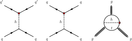
At tree level and leading order in the expansion, integrating out the Higgs induces the following non-zero initial conditions for four-quark operators (see first two diagrams in Fig. 1)
| (23) |
with . In principle, also the analogous operators with leptons are induced (, ). However, since we will rely on a fixed-order computation to predict (see below), these operators do not enter our analysis.
The matching at the electroweak scale also induces the Weinberg and dipole operators, but only at the two-loop level. The Weinberg operator obtains a two-loop initial condition at only from the top-quark operator (see third diagram in Fig. 1):
| (24) |
with defined in Eq. (39). This result agrees with Ref. [3], but is, as far as we are aware, presented here for the first time in a non-parametric form.
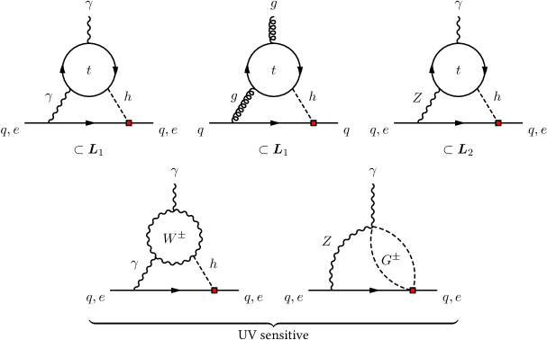
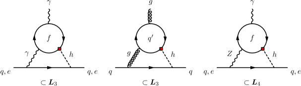
The electron photon dipole (), and light-quark photon and gluon dipoles (, with ) all receive two-loop initial conditions by integrating out the top quark and the Higgs, , and bosons:
| (25) | ||||
| (26) | ||||
| (27) |
with the precise decomposition of the coefficient functions , , and discussed below.
A few clarifications regarding Eqs. (25)–(27) are in order. We calculate the electroweak matching in fixed-order perturbation theory whenever there are no QCD corrections that are enhanced by large logarithms related to light fermion masses. This is the case for all diagrams with top-quark loops, and the diagrams with lepton loops contributing to the electron dipole, i.e. the contributions that are proportional to . (We also neglect the running of the electromagnetic coupling constant.) Therefore, the coefficients do not receive threshold contributions from virtual quarks other than the top quark, since those are properly included via the RG-mixing of the four-quark operators (Eq. (23)) into , see below. In principle, also the contributions to of all quarks other than the top should be obtained from the RG evolution; however, the corresponding mixed QED-QCD RG evolution is currently unknown222The QCD corrections to the bottom and charm contributions are naively estimated to be large (factor of a few in ) but require a more complex calculation [16].. Thus, we temporarily include the contribution of bottom and charm quarks to with a fixed-order calculation, with the understanding that corrections to these results may be large. On the other hand, we do not include the corresponding fixed-order results for the light-quark (, , ) contributions to . In addition to the issue of the large unkown QCD corrections, these contributions are suppressed by the light-quark masses. Therefore, it is not but the coefficients that provide the numerically leading constraints on the couplings for light quarks. Similarly, we do not include the contributions of the electron and muon to . The appearance of their masses (that are much smaller than the lowest scale, , where these operators can be meaningfully defined) in the logarithms would spuriously enhance the corresponding bounds by large factors. These contributions should be taken into account properly by using the RG. The tau, on the other hand, has a mass large enough to justify a fixed-order calculation as an estimate and is thus included. Note, however, that numerically the by far strongest bounds on the coefficients of all three leptons arise from the electron EDM, and their contributions to the hadronic EDMs do not play a role in our analysis, given current experimental data.
The decomposition of the coefficients , , and in Eqs. (25)–(27) are
| (28) | ||||
| (29) | ||||
| (30) |
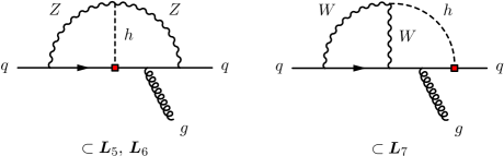
with and . and correspond to the vector and axial-vector coupling of the boson to a fermion, respectively. In Fig. 2 and Fig. 3 we show representative diagrams contributing to –. As discussed, only and contain UV sensitive electroweak contributions proportional to , thus all other scheme-dependent finite electroweak threshold corrections have been dropped in and . We have, however, kept the terms from top-quarks loops (proportional to and ) as they depend on the top-quark Yukawa and as such are independent of the scheme-dependent electroweak corrections. The loop functions () read
| (31) | ||||
| (32) | ||||
| (33) | ||||
| (34) | ||||
| (35) | ||||
| (36) | ||||
| (37) | ||||
| (38) |
where we defined the mass ratios . For the case of small fermion masses, i.e., when , we have expanded for convenience the function. Our loop functions , , correct a global factor of with respect to the corresponding ones in Ref. [5] and a typographical sign mistake in the coefficient of in in the same reference. The loop function implicitly corrects an error in Eq. (A.5) of Ref. [24], where two logarithms seem to have been incorrectly added.
The function in the results above is given by [26]
| (39) |
where , and the dilogarithm and Clausen function are defined as
| and | (40) |
respectively.
Having computed the initial conditions at the electroweak scale, we perform the QCD RGE evolution from to the hadronic scale GeV (see Refs. [3, 15] for details). For operators with quarks the RGE evolution resums large QCD logarithms and accounts for mixing among different operators. In the case of light-quark SMEFT operators, the tree-level induced four-quark operators ( and ) mix at one-loop under QCD into the quark dipoles. Nevertheless, the contributions to and of two-loop diagrams with top-quark and -boson loops provide the numerically dominant effect [19] as the four-fermion operators are additionally suppressed by an extra light-quark mass (see Eq. (23)).
The situation is different for contributions from bottom- and charm-quark SMEFT operators. Here the leading contribution to partonic dipoles (, ) and the Weinberg operator () are induced by mixing during the RG evolution. The main reason is that the nuclear matrix elements of bottom and charm dipole operators are tiny. Therefore, diagrams like the ones in Fig. 2 do not contribute, i.e., bottom and charm quarks only enter as virtual particles in loop diagrams. At the same time, their mass is significantly below the electroweak scale. For this reason, a tree-level matching at the electroweak scale and the subsequent one-loop RG evolution [23], which must include the mixing of four-fermion operators into dipole and Weinberg operators, is sufficient (and necessary) to obtain the leading-logarithmic result. The two-loop calculation has been performed in Ref. [15] but is not used in this work, as perturbative uncertainties and higher-order corrections are generally neglected in our analysis (see the discussion in Sec. 7.3).
5 Electric dipole moments
Non-zero coefficients of the higher dimension operators in Eq. (9) induce in general electric dipole moments in nucleons, atoms, and molecular systems via contributions to the hadronic Lagrangian in Eq. (12). Here we summarize the status of the induced dipole moments for the systems used in our fit, namely, the electron, neutron, and mercury EDMs.
In addition to these EDMs there are also constraints from the experimental measurement of the muon EDM [30], as well as other systems with a hadronic component. The direct constraint from the current muon EDM measurement leads to constraints that are about six orders of magnitude weaker than the one obtained via virtual muon contributions to the electron EDM, and will thus not be used. Concerning other hadronic EDMs, we have checked that within our setting the experimental bounds on the radium [31] and xenon [32] EDMs are not competitive with the neutron and mercury bounds and we do not include them in the fit either.
5.1 Electron
The most recent experimental bound on the electron EDM is [33]
| (41) |
This value was obtained using ThO molecules, neglecting any CP-violating electron–nucleon couplings. Bounds on the electron EDM have also been obtained using YbF [34] and HfF+ [35]. The resulting bounds are currently not competitive with the ThO bound and are thus not used in our fit.
5.2 Neutron
The simplest hadronic system used in our fit is the neutron. The most recent experimental bound on the neutron EDM is [36]
| (42) |
The future projections estimate an improvement of the limit to cm [36]. Throughout this work, we assume that the term has negligible effect on any EDMs and all effects arise from the Yukawa SMEFT operators. The dipole moments of the partons then contribute to the neutron EDM as
| (43) |
The hadronic matrix elements of the chromoelectric dipole operators () and the Weinberg operator () are estimated using QCD sum rules and chiral techniques [21, 20, 37]. For the matrix elements of the electric dipole operators () we use the lattice results [38] , , . The sign of the hadronic matrix element of the Weinberg operator is not known; to be definite, we choose the positive sign in our analysis. Note that in our scenario the contribution of the Weinberg operator is always subdominant (either suppressed by small quark masses, or numerically small compared to the electron EDM bound), such that the sign ambiguity does not affect the results of our global fit.
5.3 Mercury
Significant constraints in our fit arise also from the mercury EDM. The experimental bound is [39]
| (44) |
The relation of the partonic EDMs to that of mercury is given by [20]
| (45) |
Here, fm-2 denotes the contribution of the Schiff moment to the mercury EDM, with an error not exceeding 20% [40]. The expression in square brackets is the Schiff moment for mercury. The CP-odd isoscalar and isovector pion-nucleon interactions are given by fm-1, fm-1, obtained from QCD sum-rule estimates [41], while [42, 43] is the CP-even pion-nucleon coupling. The contribution of these interactions to the Schiff moment is given by the parameters fm3 and fm3. We took these “best values” from Ref. [20]; they have an intrinsic uncertainty of about an order of magnitude. The contributions of unpaired proton and neutron to the Schiff moment has been calculated in Ref. [44], with result fm2 and fm2. Finally, the contribution of the electron EDM is subdominant; no explicit uncertainty is given for the prefactor [41, 20]; however, different evaluations lead to different signs [45]. See Ref. [20] for a detailed discussion of all contributions to the mercury EDM. Employing “central values” for all parameters, we find numerically
| (46) |
with given in Eq. (43).
We have neglected several contributions in Eq. (45). The isotensor pion–nucleon coupling contributes in principle, but is expected to be small in comparison to the scalar and vector coupling, as it arises at higher order in chiral perturbation theory [20]. Contributions of four-fermion operators are smaller than the chromo EDM contributions by two orders of magnitude, and are also neglected. Finally, in our analysis we neglected the proton EDM contribution that is one order of magnitude smaller than the neutron EDM contribution, as well as the small electron EDM contribution.
6 Collider observables
The SMEFT couplings in the Lagrangian in Eq. (9) do not only induce electric dipole moments, but also affect the production cross sections and decay branching ratios of the Higgs boson. In this section we give an overview of the most important effects; the actual numerical implementation of the LHC constraints is discussed in Sec. 7. The main effects are captured by considering modifications of the gluon fusion production cross section () and the branching ratio (both are one-loop induced both in the SM and in our setup), as well as of the branching ratios to fermions observed by ATLAS and CMS (, , , ), and the total decay width of the Higgs. It is convenient to parameterise these modifications in terms of the parameters
| (47) |
Using Eq. (11) we can readily translate to the -framework parameters, i.e., and .
The deviation from the SM gluon fusion cross section or the decay to gluon-induced light jets can be effectively captured by (see Ref. [3] for details)
| (48) |
where we have defined , the sum runs over all quark flavours , and the fermionic one-loop functions are given by
| (49) |
Similarly, the modification of the Higgs decays into two photons with respect to the SM reads
| (50) |
where the sums run over all charged fermions with for quarks and for leptons, and the bosonic contribution is given by
| (51) |
with . We keep the modifications of the Higgs coupling to and bosons unmodified as the contributions from Yukawa operators are loop induced compared to the tree-level contributions already present at the dimension-four level. Moreover, is omitted as its decay width is suppressed by a smaller coupling compared to .
The signal strengths of searches for Higgs decays to fermions are also affected by the corresponding modifications of the partial widths, namely:
| (52) |
As of now, the ATLAS and CMS collaborations have observed Higgs decays into . However, the modifications of the partial widths to any fermion affect the total width of the Higgs via
| (53) |
which in turn affects all its branching ratios, i.e., all the signal strength for Higgs searches.
We conclude this section with some remarks concerning the convergence of the SMEFT expansion and the potential impact of dimension-eight operators. The issue arises because the squared amplitude enters the expression (52), leading to terms proportional to in that we keep in our numerics. What would be the impact of including dimension-eight Yukawa operators (of the generic form ) in the amplitude? While this question is hard to answer quantitatively without actually performing the analysis, the following arguments suggest that the impact would result only in minimal changes on the bounds of the dimension-six coefficients.
First, note that this issue concerns only the real parts of the Wilson coefficients. As there is no interference with the SM in the CP-odd part of the amplitude, such dimension-eight terms would be of order . The first term on the right side of Eq. (52), on the other hand, would be changed to
| (54) |
Here, and denote generic dimension-six and dimension-eight Wilson coefficients, respectively. We see that the additional last term in Eq. (54) is parametrically suppressed with respect to the linear dimension-six term by a factor , and with respect to the quadratic dimension-six term by a factor . A potential problem arises if the term quadratic in dominates the fit. A direct comparison between the last two terms in Eq. (54), under the “EFT assumption” , shows that the dimension-eight contribution will be subleading as long as . We will see in Fig. 4 that this condition is clearly satisfied for all fermions apart from the top quark. While this is only a rough estimate, we interpret this as an indication that the impact of the dimension-eight terms on the fit would be tiny. By contrast, Fig. 5 shows that for the top quark , which is larger than , such that for values of the dimension-eight term would contribute significantly to the fit. While this required value of is close to the perturbativity limit, we conclude that the EFT expansion in the collider observables might not work as well for the top quark as it does for all other fermions. CP-odd contributions, on the other hand, are not expected to receive large corrections from dimension-eight operators for any of the fermions, as discussed above.
7 Global Analyses
Having obtained in the previous sections the expressions for the relevant observables, EDMs, Higgs production cross sections (), and branching ratios (BR) decay widths we now combine the constraints on the considered Wilson coefficients in a global analysis. For this purpose we use the GAMBIT global fitting framework [12] to calculate a combined likelihood based on these two sets of constraints. The collider likelihoods are taken from the HiggsSignals_2.5.0 and HiggsBounds_5.8.0 codes [46, 47] interfaced with the ColliderBit module [13] of GAMBIT.
HiggsSignals contains three modules to compute likelihoods from Higgs measurement at the LHC. Each module calls HiggsBounds to calculate the various production cross sections and branching ratios within our SMEFT model and to obtain the signal strengths implemented in each module.
The first module computes a likelihood of Run 1 Higgs measurements using a set of signal strengths provided by the ATLAS and CMS combination of Run 1 data [48]. In this module, the signal strengths are “pure channels” in the sense that one decay channel is combined with one specific production channel, i.e., with and indicating different production modes (, VBF, , , ) and decay channels (, , , ), respectively. Run 1 data are sensitive to such signal strengths. The (Log)likelihood is then obtained from
| (55) |
where are the vectors containing the signal strengths computed as a function of the SMEFT Wilson coefficients, are the corresponding experimental combinations, and the superscript “” denotes transposition. The matrix is the signal-strength covariance matrix describing the uncertainties of and correlations among the signal strengths.
For Run 2 measurements there are two HiggsSignals modules to compute a likelihood, one that uses the simplified template cross section measurements (STXS) [49] and another that uses the peak-centered method. In our analysis we mainly use the former since the peak-centered method increases the computing time by almost an order of magnitude and has also less constraining power, as we have checked explicitly. The only exception in which we do use the peak-centered-method module is to include the two analyses containing in total peak measurements [50, 51]. Each signal strength is a combination of various production modes weighted by the corresponding experimental efficiency (), which accounts for the detector performance in identifying signal events, i.e.,
| (56) |
In our analysis we include the signal strengths of measurements originating from experimental searches from June 2021 [52, 53, 54, 55, 56, 57, 58, 59, 60, 61, 62, 63, 64, 65, 66, 67, 68, 69, 70, 71]. The corresponding (Log)likelihood is then obtained in an analogous manner as for the Run 1 data in Eq. (55). The SM predictions for the cross sections are obtained through a fit to the predictions from Yellow Report 4 [49].
To compute a likelihood from the EDM measurements, we assume their experimental uncertainties to be Gaussian distributed yielding the likelihoods ()
| (57) |
with . The uncertainties are obtained from the upper limits given in Eqs. (41), (42), and (44) by assuming zero central values for .
The total likelihood of a parameter point is computed from the sum of the values from the EDM and LHC likelihoods. To identify preferred regions in a subspace of the scanned parameters we must profile over the remaining scanned parameters. We perform the profiling using pippi [72], which computes the lowest possible value of each parameter point in the subspace of interest by allowing all other parameters to float simultaneously to minimize the . When projecting onto a two-parameter subspace, the allowed regions at 68% and 95% CL correspond to the parameter space for which the difference is less or equal than and , respectively. is the value of the best-fit point, i.e., the lowest value. In our case the value of the SM (all SMEFT Wilson coefficients are zero) divided by the number of the included observables is , where we did not include the peak observables from the measurements; they only affect the muon Yukawa. In the scan that we present the difference between the of the best-fit point and the SM is always less than , so we do not display the best-fit value in the plots.
7.1 One-flavour scans
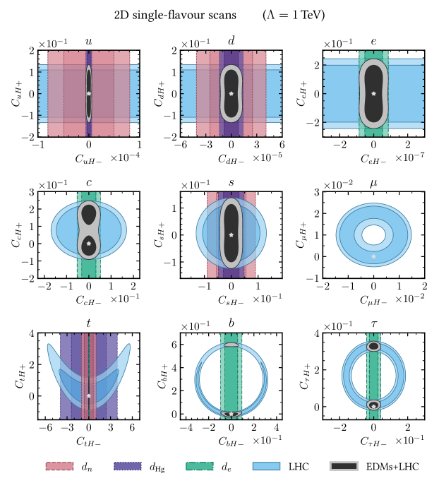
To set the stage, we first perform two-dimensional scans over the Wilson coefficients of each fermion individually, with the Wilson coefficients of all other fermions set to zero. The results are shown in Fig. 4. We allow the Wilson coefficients to float within their perturbative values, , and fix TeV in our scan. All numerical input parameters are taken from Ref. [73].
In this work, we parameterize the effects beyond the SM by the SMEFT Wilson coefficients in Eq. (9). EDMs only constrain the imaginary part of the Wilson coefficients, , while LHC observables constrain also the real parts, . In general, the electron EDM gives the strongest bounds on CP-violating parts of the lepton and heavy-quark (top, bottom, charm) coefficients, while the corresponding light-quark (up, down, strange) coefficients are mainly constrained by a combination of neutron and mercury EDM measurements.
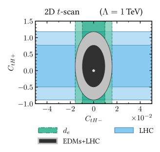
Top
The constraints from the modification of Higgs
production in gluon fusion have the parametric dependence , where we used the asymptotic values
, valid to good approximation for the top
quark, and neglected the contribution of all other quark flavours. In
the same approximation, we have . These are the dominant LHC
constraints on the top couplings; note, however, that all production
channels are included in our analysis. The corresponding constraints
are shown in Fig. 4 (bottom left panel). The strongest
individual bound on the CP-odd coefficient arises from the
electron EDM, while the constraints arising from the hadronic systems
are much weaker, see Fig. 4. A zoomed-in version of
the combined fit region is shown in Fig. 5.
Bottom, charm, tau, muon
None of the bottom, charm, tau,
and muon EDMs themselves have been measured with high
precision. Consequently, EDM bounds on CP-odd Higgs couplings of the
fermions arise from their virtual contributions to the electron EDM
(again, the bounds arising from hadronic systems are negligible in
comparison). It is remarkable that, the presence of a large quadratic
logarithm (see Eq. (33)), makes the electron EDM bound weaker
than that on the top by only a factor for the bottom, a factor
for the charm, a factor for the muon, and of the same order for
the tau, rather than being suppressed by the much larger factor , expected
naively [24] from the Yukawa suppression. For the
bottom and charm quarks, this strong logarithmic enhancement indicates
that QCD corrections are large in these cases and should be
included [16], similar to the case of hadronic dipole
moments [3, 15] (see the discussion in
Sec. 3).
Measurements at the LHC directly constrain the decay of the Higgs into bottom, charm, tau, and muon pairs. The main effect comes from the modification of the partial widths (see Eq. (52)). This is a simplified picture, as modifying any Yukawa also affects the total Higgs decay width (see Eq. (53)), the decay and, for quarks, also Higgs production via gluon-fusion. This effect is largest for the bottom quark (that dominates the SM Higgs decay width); nevertheless, we include the effect of all fermions on the total Higgs width.
Note that a negative value for the bottom Yukawa (in the sense of Eq. (11)) is excluded at CL (bottom middle panel in Fig. 4). Note also that for the muon Yukawa, the recent LHC measurements are more constraining than the electron EDM by an order of magnitude. Regarding tau couplings, the CMS analysis on the CP structure of the decay [74] disfavours large values of . While this analysis is not included here, as it is not (yet) part of the HiggsSignals data set, it would split the 2 LHC constraint (blue region in lower right panel of Fig. 4) in two distinct regions as illustrated in the CMS analysis [74].
Electron, up, down, strange
The main EDM bounds on the
electron and light-quark (up, down, strange) SMEFT coefficients arise
from their contributions to the electron EDM and the neutron and
mercury EDMs, respectively, as discussed in Sec. 4. Note
the different impact of the neutron and mercury EDMs on the up and
down coefficients, due to the strong isospin dependence of the
corresponding EDM predictions.
LHC bounds on the Wilson coefficients for the electron and the up and down quarks arise from modifications of the total Higgs decay width Eq. (53). Indeed, we checked that the contributions to gluon fusion and are subleading. (For modifications of Higgs production induced by parton distribution functions, see Ref. [75].) However, the resulting constraints are very weak when compared to the SM Yukawas, as illustrated by the corresponding ratios , , and . In contrast, the bound on the CP-odd strange-quark coefficient from LHC is almost competitive with the hadronic EDM bounds (central panel in Fig. 4).
7.2 Two-, three-flavour scans, and beyond
Next, we let the Wilson coefficients of more than one fermion flavour float simultaneously. This allows for the cancellation of the contributions of the considered Wilson coefficients to the constraining EDMs, thereby relaxing the bounds in certain regions of parameter space. There are no such cancellations possible in the collider observables, because the main effect comes from partial decay widths where no interference is possible. (The small interference term between top- and bottom-quark contribution to Higgs production via gluon fusion and is negligibly small.) However, the bounds on the different Wilson coefficients are still correlated. For instance, the Higgs decay into bottom quark dominates the total Higgs decay width, and thus the rate affects all branching ratios significantly. The same is true, albeit to a lesser extent, for all other Higgs decays.
Up and down
In the left panel of Fig. 6 we show the results of a
two-parameter scan over and . We do not scan over
the corresponding CP-even Wilson coefficients as they do not enter the
EDM predictions. The different dependence of the neutron and the
mercury EDMs on the up- and down-quark coefficients is clearly
visible. With the isoscalar pion-nucleon coupling (entering the
mercury EDM prediction) being subdominant, the bands of the two
observables are nearly orthogonal, thus allowing to set stringent
constraints on both and .
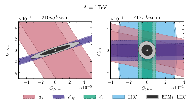
Bottom and strange
In the right panel of Fig. 6 we show the results of a
four-parameter scan over and after profiling
over the CP-even couplings. As we neglect the tiny strange-quark
contribution to the electron EDM, the only constraint on
arises from the two hadronic EDMs. On the other hand,
receives its dominant constraint from the electron EDM, while the
contributions to the hadronic EDMs are also taken into account.
We include the CP-even Wilson coefficients in the scan as they are both bounded by LHC measurements. As there is no direct measurement of , the correlation between and results from the contributions to the total Higgs decay width. The analogous plots with CP-even Wilson coefficients do not contain any additional information compared to the one-flavour scans and are thus not shown here.
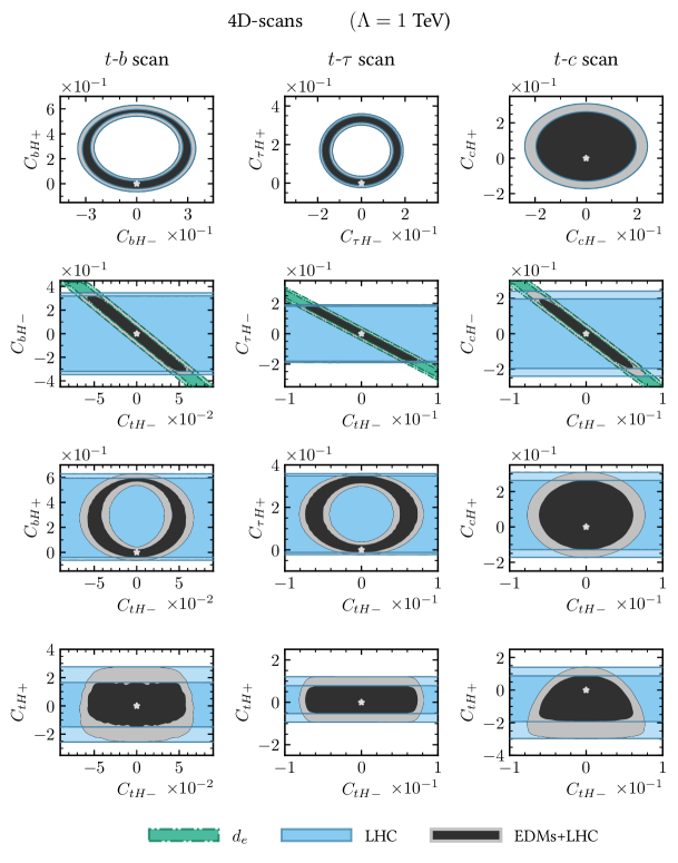
Top and bottom; top and tau; top and charm
In Fig. 7 we show the results of three different
four-parameter scans, floating simultaneously with
(first column), with (second column), and
with (third column). The electron EDM bounds on
could, in principle, be lifted by two orders of magnitude compared to
the single-flavour scan by choosing values close to the perturbativity
limit for , , and . However, given the
LHC bounds on these parameters the bound on is weakened by
only a factor of the order of five. Note also that allowing
to float significantly increases the allowed range of values for
at the CL (upper left panel in
Fig. 7). The relaxation of the bounds compared to
the single-flavour fit is even more pronounced for the charm quark
(upper right panel in Fig. 7). In the last row, we
present the constraints on the parameters and ,
with the other parameters profiled. This can be directly compared to
Fig. 5, showing a significant relaxation of
the bounds.
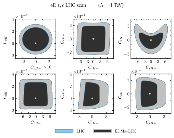
Interestingly, the combination of the electron EDM with LHC constraints has a profound impact on the constraint on the CP-even Wilson coefficients and not only on the CP-odd ones as one would naively expect. To understand this better, we first consider the second panel from above in the first column of Fig. 7 showing the allowed – region. Here, the allowed combined region corresponds to the intersection of the electron EDM and the LHC constraint, which implies that for each allowed pair of , it is possible to find corresponding allowed values of and (which have been profiled out in the plot). This can easily be verified by looking at the bottom-left and bottom-center panels of Fig. 4. By contrast, the electron EDM on its own does not constrain the – subspace at all, i.e., the whole parameter space of the third panel in the first column of Fig. 7 (– plot) is allowed with respect to the electron EDM. The reason being that one can always cancel the top against the bottom contributions to the EDM (see green band in the upper left panel). However, the combined EDM–LHC region is smaller than the one allowed by LHC alone, as not all values of required to cancel the contributions of are allowed by LHC bounds. In fact, the bottom single-flavour analysis (bottom center panel of Fig. 4) indicates that roughly , resulting in the much smaller allowed combined region in the 4D scan. Similar arguments apply to the plots that show the top–tau and top–charm coefficients. Regarding the case of the charm quark, note that its contribution to the electron EDM is larger than that of the bottom quark, while the LHC constraint is comparatively weaker, resulting in a larger allowed combined region. Finally, we remark that while the contribution to the electron EDM of the muon is similar to that of the bottom, the muon Yukawa is so strongly constrained by recent LHC measurement that no appreciable cancellation can occur, which is why we do not present this scan.
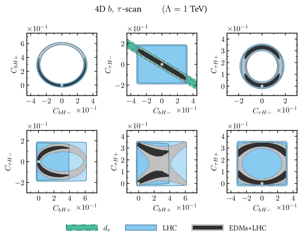
Bottom and tau
In Fig. 8 we show the results of a scan of the four
parameters and . As in the previous
four-parameter scans, there is an interesting interplay between EDM
and LHC bounds. When considering EDM bounds only, we can always cancel
the constraint if either or is
profiled. Hence, there are no pure EDM constraints in any but the
upper center panel where the CP-odd coefficients and
are displayed. In contrast, the EDM constraints cannot
always be satisfied if also LHC constraints are included. In the upper
right plot with the two tau coefficients displayed, one can see that
the allowed, combined region is enlarged compared to the
single-flavour scan. However, for extreme values for ,
still allowed by LHC bounds, cannot be profiled such that it
compensates the large tau contribution to the electron EDM and
simultaneously still be within the 2-level bottom LHC
bounds. In contrast, can be profiled such that the coefficient in the upper left plot is only bounded by LHC
constraints. The reason for this is apparent from
Eq. (25): the contribution of the tau to the electron and
quark EDMs are larger than those of the bottom by about a factor , meaning
that the bottom contribution can always be fully canceled by
contributions, but not vice versa. This implies that, given current
data, the combined bounds (apart from the combination ) are more stringent than either the LHC bounds or the EDM
bounds alone. The effect of the electron EDM, further restricting the
parameter regions allowed by LHC data, is also clearly visible in the
combined region in the lower center panel that shows the bounds on the
two CP-even coefficients and .
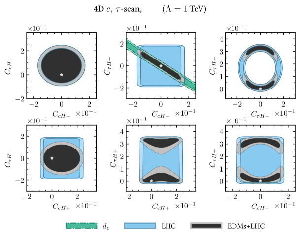
Charm and tau
In Fig. 9 we present the results of a scan of the
four parameters and . The results are
analogous to the case of bottom and tau discussed above. Note that the
contribution to the electron EDM of the charm quark is larger than
that of the bottom quark by a factor of roughly , while the LHC
bounds on the charm quark are considerably weaker that those on the
bottom quark.
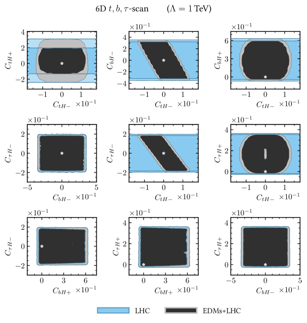
Top, bottom, and tau (third generation)
In Fig. 10 we present a scan of all six
third-generation parameters , , and
. It is interesting to compare the results to the case in
which only two out of the three flavours were included in the fit
(Fig. 7).
First, we focus on the set of the four panels (upper and middle row, center and right) that show the same parameter combinations as the panels at the same positions in Fig. 7. We see that after profiling the remaining third-generation couplings, an “indirect” electron EDM constraint on remains, although the allowed region is now significantly larger. By contrast, the “indirect” electron EDM constraint can be lifted completely by (that is only weakly constrained from LHC measurements) in the panels in the bottom row and center left of Fig. 10, leaving only the LHC constraints. This should be compared to the corresponding much smaller combined regions in Fig. 8.
The top left panel of Fig. 10 shows the constraints on both top Wilson coefficients, . Notice that the allowed values increased by about a factor of two for and by one order of magnitude for compared to the single-flavour scan (Fig. 5).
The large computational resources required for scans with more than six parameters prevent us from scanning over more than three flavours. Nevertheless, we can infer some results in this direction from the one-, two-, and three-flavour scans above. Specifically, we will consider how the constraints on the third-generation Wilson coefficients change when including more flavours in the scans.
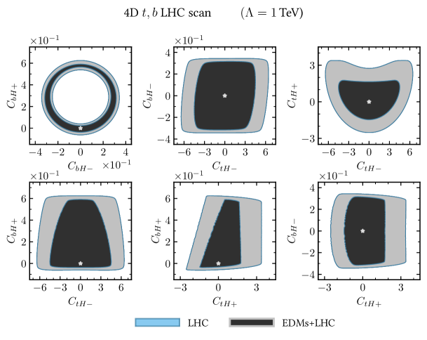
Top, bottom, (electron, light quark)
As an example, we float and under the
presumption that any contributions to EDMs can be compensated by
appropriate values of the coefficients and ,
, which we, however, do not scan over. In this way only LHC
bounds remain, which are one to two orders of magnitude weaker for
with respect to the electron EDM. The results are shown in
Fig. 11. We find that the LHC constraints on
and are somewhat lifted compared to the
single-flavour scans due to the large contribution of the bottom to
the total Higgs width, while the absence of EDM bounds allows for much
larger allowed ranges of and . The analogous
results for the charm instead of the bottom couplings are shown in
Fig. 12.
More generally, the CP-violating up, down, and electron Wilson coefficients are merely and severely constrained by EDM measurements. Hence, including , , and in a scan over the Wilson coefficients of the second or third generation would allow to completely cancel any EDM constraints and again only LHC constraints would remain.
7.3 Theory uncertainties
In this work, we did not study the impact of theoretical uncertainties on the bounds on the Wilson coefficients. Hence, a short discussion of these effects is in order. The relevant uncertainties are: (i) uncertainties in the hadronic matrix elements; and (ii) perturbative uncertainties.
(i) The uncertainties on the hadronic matrix elements have been shown in Sec. 5. Note that, in addition to the ranges given for the parameters, also some of the relative signs are not determined. In our numerical analysis, we have taken the central values for the hadronic matrix elements, and (somewhat arbitrarily) chosen the positive signs where they were not determined. We did not include these uncertainties in our likelihood function. In fact, no bounds at the CL would result from the mercury EDM, while the neutron EDM bounds would get weaker by about a factor . At CL, there would also be no bound from the neutron EDM. (In Ref. [2], much smaller effects of the hadronic uncertainties have been found. This may be related to the statistical treatment of the uncertainties; in our computation we take uncertainty on the EDMs from hadronic input, , to scale with the Wilson coefficients.) On the other hand, the bounds on the heavy quarks (top, bottom, charm) are dominated by the electron EDM that has no hadronic uncertainties. Recall also, as discussed above, that EDM constraints become less relevant upon including more Wilson coefficients in the fit, implying that the hadronic uncertainties do not (currently) play a significant role in the multi-parameter fits.
(ii) It is important to recognize that, in many cases, the perturbative uncertainties are as large as the nonperturbative uncertainties. As an example, consider the bounds on the bottom and charm Wilson coefficients, studied (within the framework) in Ref. [15]. There it was shown that the QCD corrections are large; after inclusion of the two-loop leading-logarithmic QCD corrections, the uncertainties on the electric and chomoelectric Wilson coefficients are reduced to order of . We do not include the NLO corrections here, as lattice results are not available for all required matrix elements (see Refs. [76, 77, 78] for preliminary results). Maybe somewhat surprisingly, also the electron EDM bound on the CP-violating bottom and charm Yukawas receives large QCD corrections. The calculation of these effects is ongoing [16] and also not included in this work. No theory uncertainties are included in the LHC constraints. Note that they are partially contained in the uncertainties quoted by the experiments.
8 Discussion and conclusions
In this work we have presented the first high-dimensional fits of the coefficients of Yukawa-type SMEFT operators to multiple EDMs and LHC data. As expected, upon inclusion of a sufficient number of Wilson coefficients, all EDM constraints can be evaded, and only LHC bounds remain. However, when considering the heavy fermions only, a nontrivial interplay between contributions remains.
There are several ways to further extend our analysis in the future. As discussed in Sec. 7.3, we have neglect the impact of hadronic and perturbative uncertainties on our fit results. This impact can be profound in the lower-dimensional scans, and further motivates the ongoing efforts to decrease the uncertainties.
Improved experimental bounds (or discoveries), as well as the inclusion of additional EDMs such as those of proton and deuterium, once they become available, are expected to have a significant impact on the global fit. In particular, the different isospin dependence of the various hadronic systems will help to disentangle CP-odd Higgs couplings of the first-generation quarks. The CP structure of the heavy-fermion Yukawas can be tested more directly at present and future colliders by studying observables that are designed specifically to test the CP-odd couplings and typically require a vast amount of (expected) future data (see, e.g., Refs. [79, 80, 81, 82, 83, 84, 85]).
Finally, as explained in Sec. 2 where we introduced the theoretical framework for flavour-diagonal CP-violation in Higgs Yukawas, we do in general expect new flavour violating sources to accompany beyond-the-SM CP-violation. Therefore, allowing for flavour-changing contributions within SMEFT, and including the corresponding observables would be a further extension of the current analysis. While such contributions are generically expected in realistic UV models and are expected to lead to much stronger bounds, the question is whether, given the proliferation of parameters and observables, it is not better to study selected UV models directly.
In the final stages of this work, Ref. [86] was published, presenting analyses with a similar scope as ours. We briefly comment on the differences between the two papers. In Ref. [86], the framework (discussed in this paper at the end of Sec. 2) is employed to perform multi-parameter fits to LHC data, including, in particular, the CMS CP analysis of the decay [74]. The interplay of LHC data and the electron EDM bound is discussed, but no combined fit to both LHC and EDM data is performed. By contrast, constraints that arise from considerations of electroweak baryogenesis are discussed extensively in Ref. [86]. The expression for the electron EDM (Eq. (13) in Ref. [86]) is given in numerical form and thus hard to verify. However, it seems that the gauge-boson contribution must be incorrect (either gauge-dependent or containing an implicit logarithmic dependence on the UV cutoff that is not made explicit; the cited references contain contradictory results). See our discussion in Sec. 4.
Acknowledgments
J. B. acknowledges support in part by DoE grants DE-SC0020047 and DE-SC0011784. E. S. would like to thank Luca Merlo and Robert Ziegler for helpful discussions.
Appendix A The -gauge Lagrangian
In Eq. (9) we presented the Yukawa Lagrangian that includes SMEFT modification from Yukawa operators in the mass-eigenstate basis and in unitarity gauge. In our computation we work in generic gauge. In what follows we present the relevant part of the Lagrangian, , in gauge after rotating to the mass-eigenstate basis for the fermions. We split the Lagrangian into
| (58) |
where
| (59) | ||||
| (60) | ||||
| (61) | ||||
Here, , , , and the can also contain flavour off-diagonal pieces. The corresponding Lagrangian for down-type quarks is obtained by the obvious interchanges , , , and by a reversal of sign in all terms that are odd in the Goldstone fields. Analogously, the corresponding Lagrangian for leptons is obtained from the up-type Lagrangian above by the obvious interchanges , , , , and again by reversing the sign in all terms that are odd in the Goldstone fields.
Appendix B An alternative flavour basis: real and diagonal Yukawas
There is a certain freedom of choosing the flavour basis for the SMEFT Lagrangian to use for presenting the phenomenological constraints. This freedom stems from the fact that both the dimension-four Yukawas () and the dimension-six SMEFT coefficients () contribute to the observed masses (and mixings) of fermions. As long as this is guaranteed any basis is equivalent. However, since a UV extension of the SM matched to SMEFT would in general induce contributions both to and there is no clear notion of a “better” or a more “physical” basis for . We have thus opted to present the bounds in the mass-eigenstate basis as discussed in Sec. 2 (see also Ref. [18]). The advantage of this basis is that it is the one required for computations and is also directly related to the -framework basis (see discussion around Eq. (11)). Another approach would be to attempt to provide the constraints in terms of basis-independent, i.e., Jarlskog-type, invariants (see recent Ref. [87]).
In this appendix, we discuss a different choice of basis that has been used in the literature [17]. We comment on the differences and point out a consistency condition on the Wilson coefficients in this basis that has been missed in the literature. As before, our starting point is the fermion mass term in Eq. (3):
| (62) |
with and generic, complex matrices. Now, instead of diagonalising the full matrix in parentheses, as we did, one may choose to rotate the fermion fields by a biunitary transformation that diagonalises only the dimension-four Yukawa matrices . In other words, we rotate with the transformation matrices
| (63) |
for , such that after the rotation
| (64) |
where now the matrices are diagonal and real with entries that, however, do not correspond to the observed fermion masses. The kinetic terms of quarks is also affected by the transformation in Eq. (63). At this stage this means that there is a matrix in the kinetic terms. Moreover, we have defined . In general, the matrices are not diagonal. However, similarly to the discussion of Sec. 2, one can make the UV assumption that they turn out to be complex but diagonal (or ignore off-diagonal entries). This is possible if the matrices , simultaneously diagonalise both and . Below we assume that this is the case. The analysis of Ref. [17] uses this basis, i.e., or rescalings of them, to present the phenomenological constraints on the SMEFT parameter space.
Since in general, the elements of contain phases, we still have not rotated to the mass-eigenstate basis. To this end we perform an additional (flavour-diagonal) rotation on the right-handed fields as in Ref. [17]:
| (65) |
Note that this chiral rotation leaves the kinetic term invariant. The phases are fixed such that they absorb any phase in the corresponding . Therefore after the rotation
| (66) |
Here, the are diagonal and real matrices with entries that correspond to the observed fermion masses, i.e., we have , obtained from
| (67) |
The phases are thus fixed and can be computed as functions of the physical masses and the entries via
| (68) |
As we have the restriction , this gives a consistency bound on or equivalently on .
References
- [1] S. J. Huber, M. Pospelov and A. Ritz, Electric dipole moment constraints on minimal electroweak baryogenesis, Phys. Rev. D75 (2007) 036006, [hep-ph/0610003].
- [2] Y. T. Chien, V. Cirigliano, W. Dekens, J. de Vries and E. Mereghetti, Direct and indirect constraints on CP-violating Higgs-quark and Higgs-gluon interactions, JHEP 02 (2016) 011, [1510.00725].
- [3] J. Brod, U. Haisch and J. Zupan, Constraints on CP-violating Higgs couplings to the third generation, JHEP 11 (2013) 180, [1310.1385].
- [4] W. Altmannshofer, J. Brod and M. Schmaltz, Experimental constraints on the coupling of the Higgs boson to electrons, JHEP 05 (2015) 125, [1503.04830].
- [5] J. Brod and D. Skodras, Electric dipole moment constraints on CP-violating light-quark Yukawas, JHEP 01 (2019) 233, [1811.05480].
- [6] W. Altmannshofer, S. Gori, N. Hamer and H. H. Patel, Electron EDM in the complex two-Higgs doublet model, Phys. Rev. D 102 (2020) 115042, [2009.01258].
- [7] F. Feruglio, The Chiral approach to the electroweak interactions, Int. J. Mod. Phys. A 8 (1993) 4937–4972, [hep-ph/9301281].
- [8] W. Buchmuller and D. Wyler, Effective Lagrangian Analysis of New Interactions and Flavor Conservation, Nucl. Phys. B 268 (1986) 621–653.
- [9] V. Cirigliano, W. Dekens, J. de Vries and E. Mereghetti, Is there room for CP violation in the top-Higgs sector?, Phys. Rev. D94 (2016) 016002, [1603.03049].
- [10] V. Cirigliano, W. Dekens, J. de Vries and E. Mereghetti, Constraining the top-Higgs sector of the Standard Model Effective Field Theory, Phys. Rev. D94 (2016) 034031, [1605.04311].
- [11] J. Kley, T. Theil, E. Venturini and A. Weiler, Electric dipole moments at one-loop in the dimension-6 SMEFT, 2109.15085.
- [12] GAMBIT collaboration, P. Athron et al., GAMBIT: The Global and Modular Beyond-the-Standard-Model Inference Tool, Eur. Phys. J. C 77 (2017) 784, [1705.07908].
- [13] GAMBIT collaboration, C. Balázs et al., ColliderBit: a GAMBIT module for the calculation of high-energy collider observables and likelihoods, Eur. Phys. J. C 77 (2017) 795, [1705.07919].
- [14] M. Jung and A. Pich, Electric Dipole Moments in Two-Higgs-Doublet Models, JHEP 04 (2014) 076, [1308.6283].
- [15] J. Brod and E. Stamou, Electric dipole moment constraints on CP-violating heavy-quark Yukawas at next-to-leading order, JHEP 07 (2021) 080, [1810.12303].
- [16] J. Brod and E. Stamou, A Precise Electron EDM Constraint on CP-violating Bottom and Charm Yukawas, .
- [17] E. Fuchs, M. Losada, Y. Nir and Y. Viernik, violation from , and dimension-6 Yukawa couplings - interplay of baryogenesis, EDM and Higgs physics, JHEP 05 (2020) 056, [2003.00099].
- [18] J. Alonso-González, L. Merlo and S. Pokorski, A new bound on CP violation in the lepton Yukawa coupling and electroweak baryogenesis, JHEP 06 (2021) 166, [2103.16569].
- [19] S. Weinberg, Larger Higgs Exchange Terms in the Neutron Electric Dipole Moment, Phys. Rev. Lett. 63 (1989) 2333.
- [20] J. Engel, M. J. Ramsey-Musolf and U. van Kolck, Electric Dipole Moments of Nucleons, Nuclei, and Atoms: The Standard Model and Beyond, Prog. Part. Nucl. Phys. 71 (2013) 21–74, [1303.2371].
- [21] M. Pospelov and A. Ritz, Electric dipole moments as probes of new physics, Annals Phys. 318 (2005) 119–169, [hep-ph/0504231].
- [22] G. Degrassi, E. Franco, S. Marchetti and L. Silvestrini, QCD corrections to the electric dipole moment of the neutron in the MSSM, JHEP 11 (2005) 044, [hep-ph/0510137].
- [23] J. Hisano, K. Tsumura and M. J. S. Yang, QCD Corrections to Neutron Electric Dipole Moment from Dimension-six Four-Quark Operators, Phys. Lett. B713 (2012) 473–480, [1205.2212].
- [24] G. Panico, A. Pomarol and M. Riembau, EFT approach to the electron Electric Dipole Moment at the two-loop level, JHEP 04 (2019) 090, [1810.09413].
- [25] J. A. M. Vermaseren, New features of FORM, math-ph/0010025.
- [26] A. I. Davydychev and J. B. Tausk, Two loop selfenergy diagrams with different masses and the momentum expansion, Nucl. Phys. B397 (1993) 123–142.
- [27] C. Bobeth, M. Misiak and J. Urban, Photonic penguins at two loops and dependence of , Nucl. Phys. B574 (2000) 291–330, [hep-ph/9910220].
- [28] P. Nogueira, Automatic Feynman graph generation, J. Comput. Phys. 105 (1993) 279–289.
- [29] T. Hahn, Generating Feynman diagrams and amplitudes with FeynArts 3, Comput. Phys. Commun. 140 (2001) 418–431, [hep-ph/0012260].
- [30] G. W. Bennett, B. Bousquet, H. N. Brown, G. Bunce, R. M. Carey, P. Cushman et al., Improved limit on the muon electric dipole moment, Physical Review D 80 (Sep, 2009) .
- [31] M. Bishof et al., Improved limit on the 225Ra electric dipole moment, Phys. Rev. C 94 (2016) 025501, [1606.04931].
- [32] F. Allmendinger, I. Engin, W. Heil, S. Karpuk, H.-J. Krause, B. Niederländer et al., Measurement of the permanent electric dipole moment of the atom, Phys. Rev. A 100 (Aug, 2019) 022505.
- [33] V. Andreev, D. G. Ang, D. DeMille, J. Doyle, G. Gabrielse, J. Haefner et al., Improved limit on the electric dipole moment of the electron, Nature 562 (10, 2018) 355–360.
- [34] J. J. Hudson, D. M. Kara, I. J. Smallman, B. E. Sauer, M. R. Tarbutt and E. A. Hinds, Improved measurement of the shape of the electron, Nature 473 (May, 2011) 493–496.
- [35] W. B. Cairncross, D. N. Gresh, M. Grau, K. C. Cossel, T. S. Roussy, Y. Ni et al., Precision measurement of the electron’s electric dipole moment using trapped molecular ions, Phys. Rev. Lett. 119 (Oct, 2017) 153001.
- [36] nEDM collaboration, G. Pignol and P. Schmidt-Wellenburg, The search for the neutron electric dipole moment at PSI, SciPost Phys. Proc. 5 (2021) 027, [2103.01898].
- [37] U. Haisch and A. Hala, Sum rules for CP-violating operators of Weinberg type, JHEP 11 (2019) 154, [1909.08955].
- [38] R. Gupta, B. Yoon, T. Bhattacharya, V. Cirigliano, Y.-C. Jang and H.-W. Lin, Flavor diagonal tensor charges of the nucleon from (2+1+1)-flavor lattice QCD, Phys. Rev. D98 (2018) 091501, [1808.07597].
- [39] B. Graner, Y. Chen, E. G. Lindahl and B. R. Heckel, Reduced Limit on the Permanent Electric Dipole Moment of , Phys. Rev. Lett. 116 (2016) 161601, [1601.04339].
- [40] V. A. Dzuba, V. V. Flambaum, J. S. M. Ginges and M. G. Kozlov, Electric dipole moments of Hg, Xe, Rn, Ra, Pu, and TlF induced by the nuclear Schiff moment and limits on time reversal violating interactions, Phys. Rev. A 66 (2002) 012111, [hep-ph/0203202].
- [41] M. Pospelov, Best values for the CP odd meson nucleon couplings from supersymmetry, Phys. Lett. B 530 (2002) 123–128, [hep-ph/0109044].
- [42] V. G. J. Stoks, R. Timmermans and J. J. de Swart, On the pion - nucleon coupling constant, Phys. Rev. C 47 (1993) 512–520, [nucl-th/9211007].
- [43] U. van Kolck, J. L. Friar and J. T. Goldman, Phenomenological aspects of isospin violation in the nuclear force, Phys. Lett. B 371 (1996) 169–174, [nucl-th/9601009].
- [44] V. F. Dmitriev and R. A. Sen’kov, Schiff moment of the mercury nucleus and the proton dipole moment, Phys. Rev. Lett. 91 (2003) 212303, [nucl-th/0306050].
- [45] J. S. M. Ginges and V. V. Flambaum, Violations of fundamental symmetries in atoms and tests of unification theories of elementary particles, Phys. Rept. 397 (2004) 63–154, [physics/0309054].
- [46] P. Bechtle, S. Heinemeyer, T. Klingl, T. Stefaniak, G. Weiglein and J. Wittbrodt, HiggsSignals-2: Probing new physics with precision Higgs measurements in the LHC 13 TeV era, Eur. Phys. J. C 81 (2021) 145, [2012.09197].
- [47] P. Bechtle, D. Dercks, S. Heinemeyer, T. Klingl, T. Stefaniak, G. Weiglein et al., HiggsBounds-5: Testing Higgs Sectors in the LHC 13 TeV Era, Eur. Phys. J. C 80 (2020) 1211, [2006.06007].
- [48] ATLAS, CMS collaboration, G. Aad et al., Measurements of the Higgs boson production and decay rates and constraints on its couplings from a combined ATLAS and CMS analysis of the LHC pp collision data at and 8 TeV, JHEP 08 (2016) 045, [1606.02266].
- [49] LHC Higgs Cross Section Working Group collaboration, D. de Florian et al., Handbook of LHC Higgs Cross Sections: 4. Deciphering the Nature of the Higgs Sector, 1610.07922.
- [50] ATLAS collaboration, G. Aad et al., A search for the dimuon decay of the Standard Model Higgs boson with the ATLAS detector, Phys. Lett. B 812 (2021) 135980, [2007.07830].
- [51] CMS collaboration, A. M. Sirunyan et al., Evidence for Higgs boson decay to a pair of muons, JHEP 01 (2021) 148, [2009.04363].
- [52] ATLAS collaboration, M. Aaboud et al., Search for Higgs bosons produced via vector-boson fusion and decaying into bottom quark pairs in collisions with the ATLAS detector, Phys. Rev. D 98 (2018) 052003, [1807.08639].
- [53] ATLAS collaboration, M. Aaboud et al., Search for the standard model Higgs boson produced in association with top quarks and decaying into a pair in collisions at = 13 TeV with the ATLAS detector, Phys. Rev. D 97 (2018) 072016, [1712.08895].
- [54] ATLAS collaboration, M. Aaboud et al., Measurements of gluon-gluon fusion and vector-boson fusion Higgs boson production cross-sections in the decay channel in collisions at TeV with the ATLAS detector, Phys. Lett. B 789 (2019) 508–529, [1808.09054].
- [55] ATLAS collaboration, M. Aaboud et al., Cross-section measurements of the Higgs boson decaying into a pair of -leptons in proton-proton collisions at TeV with the ATLAS detector, Phys. Rev. D 99 (2019) 072001, [1811.08856].
- [56] ATLAS Collaboration collaboration, Analysis of and production in multilepton final states with the ATLAS detector, tech. rep., CERN, Geneva, Oct, 2019.
- [57] CMS collaboration, A. M. Sirunyan et al., Evidence for the Higgs boson decay to a bottom quark–antiquark pair, Phys. Lett. B 780 (2018) 501–532, [1709.07497].
- [58] CMS collaboration, A. M. Sirunyan et al., Inclusive search for a highly boosted Higgs boson decaying to a bottom quark-antiquark pair, Phys. Rev. Lett. 120 (2018) 071802, [1709.05543].
- [59] CMS collaboration, A. M. Sirunyan et al., Search for production in the decay channel with leptonic decays in proton-proton collisions at TeV, JHEP 03 (2019) 026, [1804.03682].
- [60] ATLAS collaboration, G. Aad et al., Measurement of the production cross section for a Higgs boson in association with a vector boson in the channel in collisions at = 13 TeV with the ATLAS detector, Phys. Lett. B 798 (2019) 134949, [1903.10052].
- [61] ATLAS collaboration, G. Aad et al., Measurements of and production in the decay channel in collisions at 13 TeV with the ATLAS detector, Eur. Phys. J. C 81 (2021) 178, [2007.02873].
- [62] CMS collaboration, A. M. Sirunyan et al., Search for the Higgs boson decaying to two muons in proton-proton collisions at 13 TeV, Phys. Rev. Lett. 122 (2019) 021801, [1807.06325].
- [63] CMS collaboration, A. M. Sirunyan et al., Evidence for associated production of a Higgs boson with a top quark pair in final states with electrons, muons, and hadronically decaying leptons at 13 TeV, JHEP 08 (2018) 066, [1803.05485].
- [64] CMS Collaboration collaboration, Measurement of production in the decay channel in of proton-proton collision data at , tech. rep., CERN, Geneva, 2019.
- [65] CMS Collaboration collaboration, Measurement of the associated production of a Higgs boson with a top quark pair in final states with electrons, muons and hadronically decaying leptons in data recorded in 2017 at , tech. rep., CERN, Geneva, 2018.
- [66] CMS Collaboration collaboration, Measurements of properties of the Higgs boson in the four-lepton final state in proton-proton collisions at , tech. rep., CERN, Geneva, 2019.
- [67] CMS Collaboration collaboration, Measurements of Higgs boson production via gluon fusion and vector boson fusion in the diphoton decay channel at TeV, tech. rep., CERN, Geneva, 2019.
- [68] CMS Collaboration collaboration, Measurement of Higgs boson production and decay to the final state, tech. rep., CERN, Geneva, 2019.
- [69] ATLAS Collaboration collaboration, Measurements and interpretations of Higgs-boson fiducial cross sections in the diphoton decay channel using 139 fb-1 of collision data at = 13 TeV with the ATLAS detector, tech. rep., CERN, Geneva, Jul, 2019.
- [70] ATLAS collaboration, G. Aad et al., Higgs boson production cross-section measurements and their EFT interpretation in the decay channel at 13 TeV with the ATLAS detector, Eur. Phys. J. C 80 (2020) 957, [2004.03447].
- [71] CMS collaboration, A. M. Sirunyan et al., Measurement of the inclusive and differential Higgs boson production cross sections in the leptonic WW decay mode at 13 TeV, JHEP 03 (2021) 003, [2007.01984].
- [72] P. Scott, Pippi — painless parsing, post-processing and plotting of posterior and likelihood samples, The European Physical Journal Plus 127 (Nov, 2012) .
- [73] Particle Data Group collaboration, P. Zyla et al., Review of Particle Physics, PTEP 2020 (2020) 083C01.
- [74] CMS collaboration, A. Tumasyan et al., Analysis of the CP structure of the Yukawa coupling between the Higgs boson and leptons in proton-proton collisions at = 13 TeV, 2110.04836.
- [75] Y. Soreq, H. X. Zhu and J. Zupan, Light quark Yukawa couplings from Higgs kinematics, JHEP 12 (2016) 045, [1606.09621].
- [76] T. Bhattacharya, V. Cirigliano, R. Gupta, E. Mereghetti and B. Yoon, Dimension-5 CP-odd operators: QCD mixing and renormalization, Phys. Rev. D92 (2015) 114026, [1502.07325].
- [77] T. Bhattacharya, V. Cirigliano, R. Gupta and B. Yoon, Quark Chromoelectric Dipole Moment Contribution to the Neutron Electric Dipole Moment, PoS LATTICE2016 (2016) 225, [1612.08438].
- [78] B. Yoon, T. Bhattacharya, V. Cirigliano and R. Gupta, Neutron Electric Dipole Moments with Clover Fermions, PoS LATTICE2019 (2020) 243, [2003.05390].
- [79] R. Harnik, A. Martin, T. Okui, R. Primulando and F. Yu, Measuring CP violation in at colliders, Phys. Rev. D88 (2013) 076009, [1308.1094].
- [80] F. Demartin, F. Maltoni, K. Mawatari, B. Page and M. Zaro, Higgs characterisation at NLO in QCD: CP properties of the top-quark Yukawa interaction, Eur. Phys. J. C 74 (2014) 3065, [1407.5089].
- [81] M. R. Buckley and D. Goncalves, Boosting the Direct CP Measurement of the Higgs-Top Coupling, Phys. Rev. Lett. 116 (2016) 091801, [1507.07926].
- [82] A. V. Gritsan, R. Röntsch, M. Schulze and M. Xiao, Constraining anomalous Higgs boson couplings to the heavy flavor fermions using matrix element techniques, Phys. Rev. D 94 (2016) 055023, [1606.03107].
- [83] D. Azevedo, A. Onofre, F. Filthaut and R. Gonçalo, CP tests of Higgs couplings in semileptonic events at the LHC, Phys. Rev. D 98 (2018) 033004, [1711.05292].
- [84] C. Grojean, A. Paul and Z. Qian, Resurrecting with kinematic shapes, JHEP 04 (2021) 139, [2011.13945].
- [85] T. Martini, R.-Q. Pan, M. Schulze and M. Xiao, Probing the CP structure of the top quark Yukawa coupling: Loop sensitivity versus on-shell sensitivity, Phys. Rev. D 104 (2021) 055045, [2104.04277].
- [86] H. Bahl, E. Fuchs, S. Heinemeyer, J. Katzy, M. Menen, K. Peters et al., Constraining the CP structure of Higgs-fermion couplings with a global LHC fit, the electron EDM and baryogenesis, 2202.11753.
- [87] Q. Bonnefoy, E. Gendy, C. Grojean and J. T. Ruderman, Beyond Jarlskog: 699 invariants for CP violation in SMEFT, 2112.03889.