Abstract

In this paper, we propose a meshless method of computing eigenvalues and eigenfunctions of a given surface embedded in $\mathbb{R}^{3}$. We use point cloud data as input and generate the lattice approximation for some neighborhood of the surface. We compute the eigenvalues and eigenvectors of the cubic lattice graph as an approximation of the eigenvalues and eigenfunctions of the Laplace-Beltrami operator on the surface. We perform extensive numerical experiments on surfaces with various topology and compare our computed eigenvalues from point cloud surface with exact solutions and standard finite element methods using triangle mesh.

1 Introduction

For a given surface, the associated Laplace-Beltrami operator is a useful tool that describes in part the intrinsic geometric information of the shape. In particular, the eigenvalues and eigenfunctions of the Laplace-Beltrami operator, i.e., the spectrum information, are employed as global shape descriptors.

Computing eigenvalues and eigenfunctions for surfaces has a wide range of applications in mathematics and computer graphics. In mathematics, it has long been a fundamental problem to study the connections between eigenvalues and other geometric quantities such as genus and the Cheeger constants [26]. Since the analytic solutions of most eigenvalue problems are only known for special cases and usually involve meticulous analysis solving partial differential equations, a numerical algorithm for computing the eigenvalues and eigenfunctions could play an important role in discovering and verifying mathematical theorems on eigenvalue problems.

In computer graphics, computing eigenvalues and eigenfunctions is a fundamental step in spectral shape analysis. The eigenvalues and eigenfunctions could be used to measure the difference between the intrinsic geometries of the two surfaces. This is particularly useful for non-rigid shapes in 3-dimensional space. Furthermore, eigenvalues and eigenvectors could be used for surface registrations [8]. See [1] [3] [17] [18][23] for examples of such applications.

1.1 Contributions

Most existing methods for computing eigenvalues and eigenfunctions rely on the triangle mesh approximation of a surface; see [19][8]. The advantages of the point cloud-based eigenvalue method are:

• Point cloud data uses only coordinate information, which can be regarded as a subset of the information contained in a triangle mesh as the set of vertices. Comparing the accuracy of computed eigenvalues between mesh-based algorithm and meshless algorithm reveals in part the impact of surface information, which is of great theoretical importance.

• Collecting point cloud data is convenient. Contemporary 3D scanners provide 3D point cloud data sampled from the surfaces of solid objects, and mobile devices with depth sensors can collect point cloud data also. Since generating meshes from point cloud may not be feasible, algorithms computing eigenvalues directly from point cloud data are useful.

• The concept of lattice approximation could be easily generalized to higher-dimensional cases and less regular geometric objects, such as orbifolds.

In this article, we approximate a surface $M\subset\mathbb{R}^{3}$ by a point cloud, and we compute the eigenvalues of the Laplacian on a surface $M$ by approximating the $\epsilon$-neighborhood of the surface, then we compute the discrete Laplacian using the lattice. We visualize the convergence of computed discrete eigenvalues toward exact eigenvalues solved analytically.

1.2 Related works

Reuter et al. [19] introduced the spectrum of the Laplace-Beltrami operator of a shape as the signature or fingerprint of the shape. Since the spectrum is an isometry invariant, it is independent of the object’s representation, including parametrization and spatial position. The authors pointed out that in spectrum methods, checking if two objects are isometric needs no prior alignment (registration/localization) of the objects but only a comparison of their spectra. Moreover, the authors demonstrated that it is computationally feasible to extract elementary geometrical data such as the volume, the boundary length, and even the Euler characteristic from the numerically calculated eigenvalues. This indicates the geometrical importance of the eigenvalues and eigenfunctions. It is also suggested in [19] to implement spectrum methods to support copyright protection, database retrieval, and quality assessment of digital data that represent surfaces and solids. Rustamov [21] proposed to use the eigenvalues and eigenfunctions of surfaces to do shape clustering and classification. Lev́y [12] studied the specific type of function bases defined by the eigenfunctions of the Laplace-Beltrami operator. Such a function basis is well-adapted to the geometry and the topology of the object.

Dong et al. [5], Lev́y [12], and Reuter [16] used eigenfunctions to develop approaches to segment shapes. The resulting patches are well-shaped and arise naturally from the intrinsic properties of the surface. Such approaches work for any surface, regardless of its genus. In [16], algorithms are developed to segment surfaces into meaningful parts and to register these parts across populations of near intrinsic isometric shapes, such as heads, arms, legs, and fingers of humans in different body postures. The method utilized the fact that quantitative and qualitative behaviors of the eigenvalues and eigenfunctions are similar for near intrinsic isometric shapes. Topological features (level sets and Morse theory) are implemented for the segmentation. For the purpose of eliminating topological noise and comparing eigenfunctions, concepts from persistent homology are employed. [16] also discussed the computation of eigenfunctions and eigenvalues using cubic finite elements on triangle meshes and constructing persistence diagrams by the Morse-Smale complex.

In [16], the registration of the shapes is mainly for near isometric surfaces. In reality, it is often needed to find the registration of surfaces that are not near isometric. For example, heart motion and brain development are not isometric. Therefore, it could be challenging to implement the Laplace spectrum methods in these applications. Shi et al. [24] developed a novel technique for surface deformation and mapping in the high-dimensional Laplace-Beltrami embedding space. For a surface, the authors deformed its Laplace-Beltrami eigenvalues and eigenfunctions and realized its deformation in the high-dimensional Laplace-Beltrami embedding space by iteratively optimizing conformal metrics. By this deformation technique, the authors developed an approach for surface mapping between non-isometric surfaces and demonstrated its application in mapping hippocampal atrophy of multiple sclerosis (MS) patients with depression [24]. Hamidian et al. [7][9] also described an approach using eigenvalues and eigenfunctions to quantify and visualize non-isometric deformations of surfaces. Such deformation could be expressed as a linear interpolation of eigenvalues of the two surfaces, realized by a time-dependent scale function defined on each vertex. Each iteration amounts to solving a quadratic programming problem based on a spectrum variation theorem and a smoothness energy constraint. The final scale function can be obtained by combining the deformations from each step and quantitatively describing non-isometric deformations between two shapes.

There are other works that employ the spectrum of Laplacian for surface matching. Rodolà et al. [20] used perturbation analysis to show how the Laplace-Beltrami eigenfunctions change after removing part of the shape and exploited it as a prior on the spectral representation of the correspondence between non-rigid shapes. Litany et al. [13] extended the study of partial matching, including the presence of topological noise. Kovnatsky et al. [11] showed how to modify (align) the eigenvectors of the Laplace-Beltrami operator to match non-isometric surfaces. Ovsjanikov et al. [15] described a spectral method for shape matching by finding an alignment between eigenfunctions based on linear constraints. In [22][27], visualization of shape deformations based on spectral representations of the correspondence was shown. In [8], the authors used both eigenvalues and eigenvectors to align two manifolds and extracted feature points from eigenvectors and employed them to align two surfaces.

Acknowledgments. The authors would like to thank Cliff Taubes for a great deal of inspiration from his work and fruitful discussions regarding the analytic solution and all aspects of this paper. The computations in this paper were run on the FASRC Cannon cluster supported by the FAS Division of Science Research Computing Group at Harvard University. The work is also supported in part by NSF 1760471.

2 Analytic Solution of Surface Laplace’s Equation

In this section, we present analytic solutions of Laplace’s equation of a sphere and a cone. Since the analytic solutions provide the exact values of eigenvalues of surface Laplacian, they can serve as the ground truth for the evaluation and comparison of the accuracy and convergence of numerical eigenvalues obtained by different algorithms.

2.1 Spherical Harmonics

Spherical harmonics are functions defined on the surface of a sphere. They form a complete set of orthogonal functions and thus an orthonormal basis. Each function defined on the surface of a sphere can be written as a sum of these spherical harmonics. Spherical harmonics may be organized by spatial angular frequency, and they are basis functions for irreducible representations of $SO(3)$.

Spherical harmonics can be defined as homogeneous polynomials of degree $\ell$ in $(x,y,z)$ that obey Laplace’s equation. A specific set of spherical harmonics, denoted ${\displaystyle Y_{\ell}^{m}(\theta,\varphi)}$, forms an orthogonal system and is known as Laplace’s spherical harmonics. Laplace’s equation imposes that the Laplacian of a scalar field $f:\mathbb{R}^{3}\to\mathbb{C}$ is zero. In spherical coordinates, this is [4]:

$$\nabla^{2}f={\frac{1}{r^{2}}}{\frac{\partial}{\partial r}}\left(r^{2}{\frac{\partial f}{\partial r}}\right)+{\frac{1}{r^{2}\sin\theta}}{\frac{\partial}{\partial\theta}}\left(\sin\theta{\frac{\partial f}{\partial\theta}}\right)+{\frac{1}{r^{2}\sin^{2}\theta}}{\frac{\partial^{2}f}{\partial\varphi^{2}}}=0$$

with angular solutions:

$$Y_{\ell}^{m}:S^{2}\to\mathbb{C}$$

as a product of trigonometric functions. To find solutions of the form $f(r,\theta,\varphi)=R(r)Y(\theta,\varphi)$, we use separation of variables resulting in two differential equations:

$${\frac{1}{R}}{\frac{d}{dr}}\left(r^{2}{\frac{dR}{dr}}\right)=\lambda,$$

$${\frac{1}{Y}}{\frac{1}{\sin\theta}}{\frac{\partial}{\partial\theta}}\left(\sin\theta{\frac{\partial Y}{\partial\theta}}\right)+{\frac{1}{Y}}{\frac{1}{\sin^{2}\theta}}{\frac{\partial^{2}Y}{\partial\varphi^{2}}}=-\lambda.$$

This system of equations provides a solution of the Laplace equation:

$$\nabla^{2}f ={\frac{1}{r^{2}}}{\frac{\partial}{\partial r}}\left(r^{2}{\frac{\partial RY}{\partial r}}\right)+{\frac{1}{r^{2}\sin\theta}}{\frac{\partial}{\partial\theta}}\left(\sin\theta{\frac{\partial RY}{\partial\theta}}\right)+{\frac{1}{r^{2}\sin^{2}\theta}}{\frac{\partial^{2}RY}{\partial\varphi^{2}}}=0.$$

$Y^{m}_{\ell}$ can be represented as a complex exponential, and associated Legendre polynomials:

$$Y_{\ell}^{m}(\theta,\varphi)=Ne^{im\varphi}P_{\ell}^{m}(\cos{\theta}),$$

that fulfill:

$$r^{2}\nabla^{2}Y_{\ell}^{m}(\theta,\varphi)=-\ell(\ell+1)Y_{\ell}^{m}(\theta,\varphi).$$

Here $\displaystyle Y_{\ell}^{m}:S^{2}\to\mathbb{C}$ is called a spherical harmonic function of degree $\ell$ and order $m$, $P_{\ell}^{m}:[-1,1]\to\mathbb{R}$ is an associated Legendre polynomial, $N$ is a normalization constant, and $\theta\in[0,\pi]$ and $\varphi\in[0,2\pi)$ represent colatitude and longitude, respectively. For a fixed integer $\ell$, every solution $Y^{\ell}_{m}(\theta,\varphi):S^{2}\to\mathbb{C}$, of the eigenvalue problem

$$r^{2}\nabla^{2}Y^{\ell}_{m}=-\ell(\ell+1)Y^{\ell}_{m}$$ (1)

is a linear combination of $Y^{\ell}_{m}:S^{2}\to\mathbb{C}$. There are $2\ell+1$ linearly independent such polynomials. The multiplicity of the eigenvalues on a sphere equals the dimension of the space of homogenous, harmonic polynomials of degree $\ell$ [25]. Therefore, the multiplicity of the eigenvalue $-\ell(\ell+1)$ is $2\ell+1$.

2.2 Analytic Solution of Surface Laplace’s Equation on a Cone

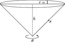
In this section, we first present the analytic solution of Laplace’s equation on the surface of a cone centered at the origin with base radius $r=1$ at height $z=1$, as illustrated in Fig. 1. We solve for the analytic solution of surface Laplace’s equation on a cone by equating Laplace’s equation and its first-order derivative on the side and top of the cone.

Figure 1: Cone centered at the origin with base radius $r=1$ at height $z=1$.

Equation on the side of the cone.

We parameterize the side of the cone as:

$$(t,\theta)\mapsto(t\cos\theta,t\sin\theta,ht),\quad 0\leq t\leq 1,\quad 0\leq\theta\leq 2\pi.$$

Then we have the metric matrix:

$$g=\begin{pmatrix}dt&d\theta\\ \end{pmatrix}\begin{pmatrix}\langle g_{t},g_{t}\rangle&\langle g_{t},g_{\theta}\rangle\\ \langle g_{\theta},g_{t}\rangle&\langle g_{\theta},g_{\theta}\rangle\\ \end{pmatrix}\begin{pmatrix}dt\\ d\theta\end{pmatrix}=(1+h^{2})dt^{2}+t^{2}d^{2}\theta.$$

Now we change the variables:

$$s=t\sqrt{1+h^{2}}\Rightarrow g=ds^{2}+{s^{2}\over 1+h^{2}}d^{2}\theta,$$

and the respective first fundamental form can be found in:

$$g=ds^{2}+{s^{2}\over 1+h^{2}}d^{2}\theta=\begin{pmatrix}ds&d\theta\\ \end{pmatrix}\begin{pmatrix}1&0\\ 0&{s^{2}\over 1+h^{2}}\\ \end{pmatrix}\begin{pmatrix}ds\\ d\theta\end{pmatrix}.$$

The inverse metric tensor is:

$$g^{-1}=\begin{pmatrix}1&0\\ 0&{1+h^{2}\over s^{2}}\\ \end{pmatrix}.$$

The Laplacian is:

$$\Delta={1\over\sqrt{\det g}}{\partial\over\partial x^{i}}\left(g^{ij}\sqrt{\det g}{\partial\over\partial x^{i}}\right),$$

so in our case,

$$\Delta ={1\over s}{\partial\over\partial s}+{\partial^{2}\over\partial s^{2}}+{1+h^{2}\over s^{2}}{\partial^{2}\over\partial\theta^{2}}.$$

Therefore, to find the Laplace eigenvalues on the side of a cone, we solve:

$${1\over s}f_{s}+f_{ss}+{1+h^{2}\over s^{2}}f_{\theta\theta}=-Ef.$$

Since $f$ is a smooth function, we can write it as:

$$f=\sum_{n=0}a_{n}(s)e^{in\theta}.$$

Since $e^{in\theta}$s are linearly independent, this is equivalent to solving:

$${1\over s}\left(a_{n}(s)e^{in\theta}\right)_{s}+\left(a_{n}(s)e^{in\theta}\right)_{ss}+{1+h^{2}\over s^{2}}\left(a_{n}(s)e^{in\theta}\right)_{\theta\theta}=-E\left(a_{n}(s)e^{in\theta}\right).$$

So we have:

$${1\over s}(a_{n})_{s}+(a_{n})_{ss}-{n^{2}(1+h^{2})\over s^{2}}(a_{n})_{\theta\theta}=-Ea_{n}$$ (2)

for each $n$.

The Bessel differential equation is the linear second-order ordinary differential equation given by:

$$x^{2}{d^{2}y\over dx^{2}}+x{dy\over dx}+(x^{2}-n^{2})y=0.$$

Therefore, rearranging Equation (2) gives the Bessel differential equation:

$$s(a_{n})_{s}+s^{2}(a_{n})_{ss}-\left(n^{2}(1+h^{2})+Es^{2}\right)(a_{n})_{\theta\theta}=0$$

with solution $J_{x}\left(\sqrt{E}s\right)$ for $x^{2}=(1+h^{2})n^{2}=2n^{2}$. Change of variable by $x=s\sqrt{E}$, so ${d\over dx}={d\over d(s\sqrt{E})}={1\over\sqrt{E}}{d\over ds}$ and ${d^{2}\over dx^{2}}={1\over\sqrt{E}}{d\over ds}{1\over\sqrt{E}}{d\over ds}={1\over E}{d^{2}\over ds^{2}}$. Then

$$s^{2}E{1\over E}{d^{2}a_{n}\over ds^{2}}+s\sqrt{E}{1\over\sqrt{E}}{da_{n}\over ds}+(s^{2}E-n^{2})a_{n}=0,$$

which simplifies to:

$$s^{2}{d^{2}a_{n}\over ds^{2}}+s{da_{n}\over ds}+(s^{2}E-n^{2})a_{n}=0.$$ (3)

Equation on the top of the cone.

We parameterize the top of the cone as:

$$(r,\theta)\mapsto(r\cos\theta,r\sin\theta,1),\quad 0\leq r\leq 1,\quad 0\leq\theta\leq 2\pi.$$

Then the metric matrix is:

$$g=\begin{pmatrix}dr&d\theta\\ \end{pmatrix}\begin{pmatrix}\langle g_{r},g_{r}\rangle&\langle g_{r},g_{\theta}\rangle\\ \langle g_{\theta},g_{r}\rangle&\langle g_{\theta},g_{\theta}\rangle\\ \end{pmatrix}\begin{pmatrix}dr\\ d\theta\end{pmatrix}=\begin{pmatrix}dr&d\theta\\ \end{pmatrix}\begin{pmatrix}1&0\\ 0&r^{2}\\ \end{pmatrix}\begin{pmatrix}dr\\ d\theta\end{pmatrix}=dr^{2}+r^{2}d^{2}\theta.$$

So the determinant of the first fundamental form is $r^{2}$, and the inverse metric tensor is:

$$g^{-1}=\begin{pmatrix}1&0\\ 0&{1\over r^{2}}\\ \end{pmatrix}.$$

Thus, the Laplacian is:

$$\Delta ={1\over r}{\partial\over\partial r}\left(r{\partial\over\partial r}\right)+{1\over r}{\partial\over\partial\theta}\left({1\over r}{\partial\over\partial\theta}\right).$$

Therefore, to find the Laplace eigenvalues on the top of a cone, we solve:

$${1\over r}v_{r}+v_{rr}+{1\over r^{2}}v_{\theta\theta}=-Ev.$$

Since $v$ is a smooth function, we can write it as:

$$v=\sum_{m=0}b_{m}(s)e^{im\theta}.$$

Since $e^{im\theta}$s are linearly independent, this is equivalent to solving:

$${1\over r}\left(b_{m}e^{im\theta}\right)_{r}+\left(b_{m}e^{im\theta}\right)_{rr}+{1\over r^{2}}\left(b_{m}e^{im\theta}\right)_{\theta\theta}=-E\left(b_{m}e^{im\theta}\right).$$ (4)

Rearranging gives the Bessel differential equation:

$$r(b_{m})_{r}+r^{2}(b_{m})_{rr}+\left(Er^{2}-m^{2}\right)(b_{m})_{\theta\theta}=0$$ (5)

with a solution $J_{m}\left(\sqrt{E}r\right)$, so $b_{m}=\alpha J_{m}\left(\sqrt{E}r\right)$ for some constant $\alpha$.

Because the solution to the respective Laplace equations on the side of the cone and on the top of the cone have to agree on the edge to be continuous, the solutions to Equations (3) and (5) have to be the same at $r=1$. There is also a continuity condition on their derivatives at $r=1$, that is, $a_{n}=b_{m}$ for $m=n$.

$$a_{n} =\left.J_{\sqrt{2}n}\left(\sqrt{E}s\right)\right|_{s=t\sqrt{1+h^{2}}\text{ at }t=1}=J_{\sqrt{2}n}\left(\sqrt{2E}\right),$$

$$b_{m} =\left.\alpha J_{m}\left(\sqrt{E}r\right)\right|_{r=1}=\alpha J_{m}\left(\sqrt{E}\right).$$

This gives the restraint:

$$J_{\sqrt{2}n}\left(\sqrt{2E}\right)=\alpha J_{n}\left(\sqrt{E}\right).$$ (6)

And also their first derivatives:

$$a^{\prime}_{n} =J^{\prime}_{\sqrt{2}n}\left(\sqrt{2E}\right),$$

$$b^{\prime}_{m} =\alpha J^{\prime}_{m}\left(\sqrt{E}\right),$$

which gives the restraint:

$$-J^{\prime}_{\sqrt{2}n}\left(\sqrt{2E}\right)=\alpha J^{\prime}_{n}\left(\sqrt{E}\right)$$ (7)

because ${\partial\over\partial r}$ points outward from the boundary of the disk, so it corresponds to $-{\partial\over\partial s}$, which points in from the top of the cone. Bring Equation (6) into Equation (7) gives the analytic solution of surface Laplacian on a cone:

$$J^{\prime}_{\sqrt{2}n}\left(\sqrt{2E}\right)J_{n}\left(\sqrt{E}\right)+J_{\sqrt{2}n}\left(\sqrt{2E}\right)J^{\prime}_{n}\left(\sqrt{E}\right)=0.$$ (8)

Using the recurrence relation:

$$J^{\prime}_{v}(z)=-J_{v+1}(z)+{v\over z}J_{v}(z),$$ (9)

we obtain the analytic solution, displayed in Table 9.

Multiplicities.

According to Equation (4), each solution $E$ of Equation (8) corresponds to two eigenvalues after expanding $e^{im\theta}$ into the real part and imaginary part for all $n>0$. Therefore, the solution from Bessel $J_{0}$ functions has multiplicity 1, and all others have multiplicity 2. Analytic solutions are exhibited in Table 10.

3 Methods of Computing Eigenvalues of Surfaces

In this section, we describe the classical method [17] for computing eigenvalues and eigenfunctions of surfaces embedded in $\mathbb{R}^{3}$ (Algorithm 1). Then we introduce an algorithm computing eigenvalues using a lattice that is approximated based on the triangle mesh (Algorithm 2), followed by our main algorithm, which computes eigenvalues using a lattice that is approximated based on the point cloud (Algorithm 3). A recent embedding method, the Closet Point Method for computing solutions to a variety of partial differential equations based on closest point representation of surface [14], is analogous to our lattice approximation. Similarly, [2] solved eigenvalues of an elliptic operator defined on a compact hypersurface in ⁿ via computing an elliptic eigenvalue problem in a bounded domain on the Cartesian grid.

3.1 Classical Method Using Triangle Mesh

We first describe the classical method of computing eigenvalues on a triangle mesh surface by Reuter [17]. Given a triangle mesh $T=(V,E,F)$ embedded in $\mathbb{R}^{3}$, one of the most well-known notions of discrete Laplacian on this piecewise linear surface is the so-called cotangent Laplacian. For any $f\in\mathbb{R}^{V}$, its cotangent Laplacian $L$ is defined as

$$(Lf)_{i}=\sum_{j:ij\in E}w_{ij}(f_{j}-f_{i}),$$

where

$$w_{ij}=\cot\alpha_{ij}+\cot\beta_{ij}$$

where $\alpha_{ij}$ and $\beta_{ij}$ are two inner angles in $(T,E,F)$ that are facing the edge $ij$.

Algorithm 1 Computing eigenvalues and eigenvectors of surfaces

Input: A triangle mesh $T=(V,E,F)$ and the number $k$ of wanted eigenvalues and eigenvectors.
Output: First $k$ non-zero eigenvalues and associated eigenvectors.

1:Compute the inner angles of $T=(V,E,F)$.

2:Compute the (normalized) sparse matrix of the cotangent Laplacian $L$.

3:Compute the first $k$ non-zero eigenvalues and associated eigenvectors of $L$.

3.2 Lattice Approximation Method Using Triangle Mesh

Given a triangle mesh $T=(V,E,F)$ embedded in $\mathbb{R}^{3}$, for a relatively small $r>0$ and a sufficiently dense cubic lattice $(\mathbb{Z}/n)^{3}$, we can take $V^{\prime}=B_{r}(T)\cap(\mathbb{Z}/n)^{3}$ as a lattice approximation. Then, we approximate the surface Laplacian by the standard graph Laplacian on the standard cubic lattice graph upon $V^{\prime}$ defined as:

$$L_{i,j}=\begin{cases}\deg(v_{1})&\text{ if }i=j\\ -1&\text{ if }i\neq j\text{ and }v_{i}\text{ is adjacent to }v_{j}\\ 0&\text{ otherwise.}\\ \end{cases},$$ (10)

Algorithm 2 Computing eigenvalues and eigenvectors of surfaces

Input: A triangle mesh $T=(V,E,F)$, and a radius parameter $r>0$, and a lattice density parameter $n\in\mathbb{Z}^{+}$, and the number $k$ of wanted eigenvalues and eigenvectors.
Output: First $k$ non-zero eigenvalues and associated eigenvectors.

1:Compute the set $V^{\prime}$ of lattice vertices in the $r$-neighborhood of the triangle mesh $T$.

2:Compute the (normalized) sparse matrix of the graph Laplace $L$.

3:Compute the first $k$ non-zero eigenvalues and associated eigenvectors of $L$.

3.3 Meshless Algorithm

Given a point cloud $P$ in $\mathbb{R}^{3}$, then for a relatively small $r>0$ and a sufficiently dense cubic lattice $(\mathbb{Z}/n)^{3}$, we can take $V=B_{r}(P)\cap(\mathbb{Z}/n)^{3}$ as a lattice approximation. Further, we approximate the surface Laplacian by the standard graph Laplacian on the standard cubic lattice graph upon $V$.

Algorithm 3 Computing eigenvalues and eigenvectors of surfaces

Input: A point cloud $P$, and a radius parameter $r>0$, and a lattice density parameter $n\in\mathbb{Z}^{+}$, and the number $k$ of wanted eigenvalues and eigenvectors.
Output: First $k$ non-zero eigenvalues and associated eigenvectors.

1:Compute the set $V$ of lattice vertices as described in Section 2.1.

2:Compute the (normalized) sparse matrix of the graph Laplace $L$.

3:Compute the first $k$ non-zero eigenvalues and associated eigenvectors of $L$.

4 Numerical Results on Surface Eigenvalues

4.1 Convergence About $r$-neighborhood and Lattice Density on Sphere

We display the computed first ten non-zero eigenvalues of $S^{2}$. Further experiments indicate that Algorithm 2 and Algorithm 3 give good approximations of the eigenvalues of $S^{2}$, as $n\rightarrow\infty$ for properly chosen $r>0$. We also did numerical experiments for different point cloud approximations of $S^{2}$, and converging speeds were different for different point clouds. The point cloud we used for $S^{2}$ is exhibited in Fig. 2.

Figure 2: (Left) point cloud of $S^{2}$; (right) triangle mesh of $S^{2}$.

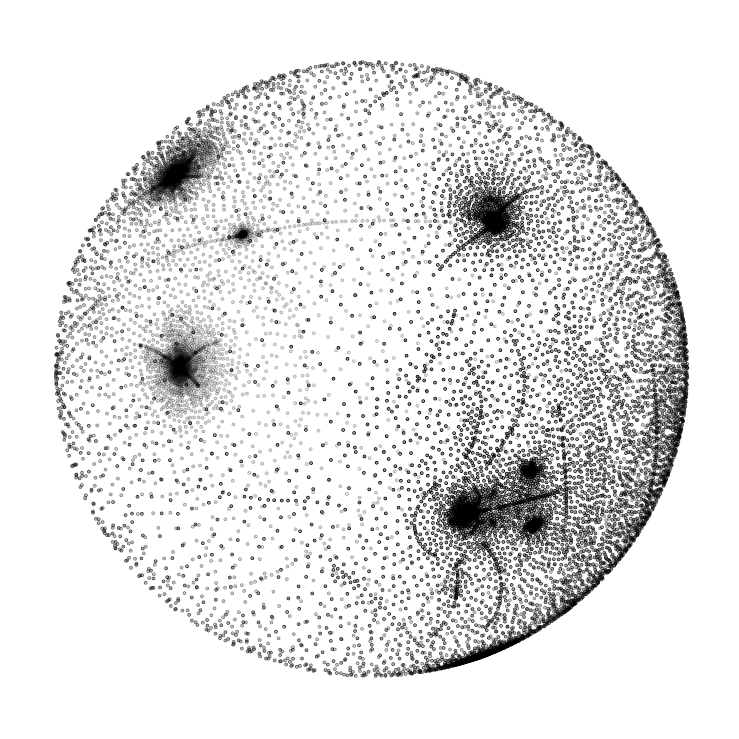
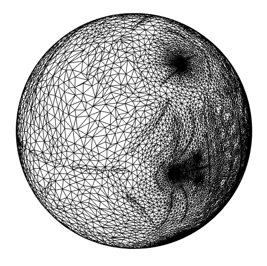
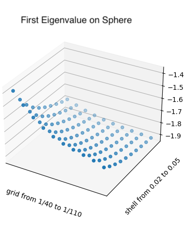
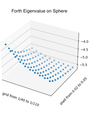
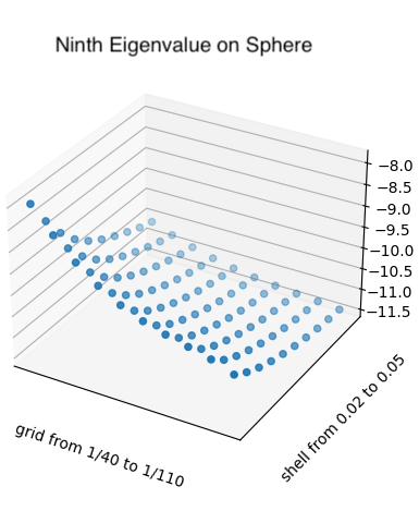
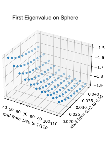
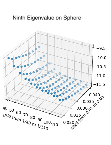
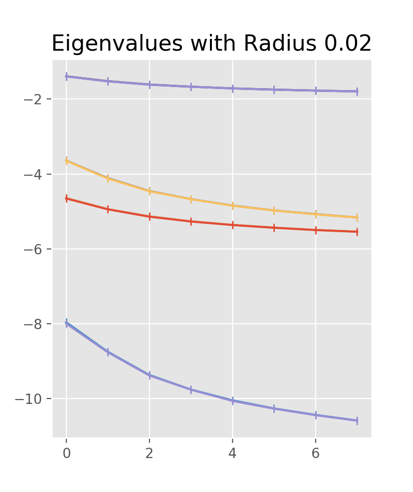
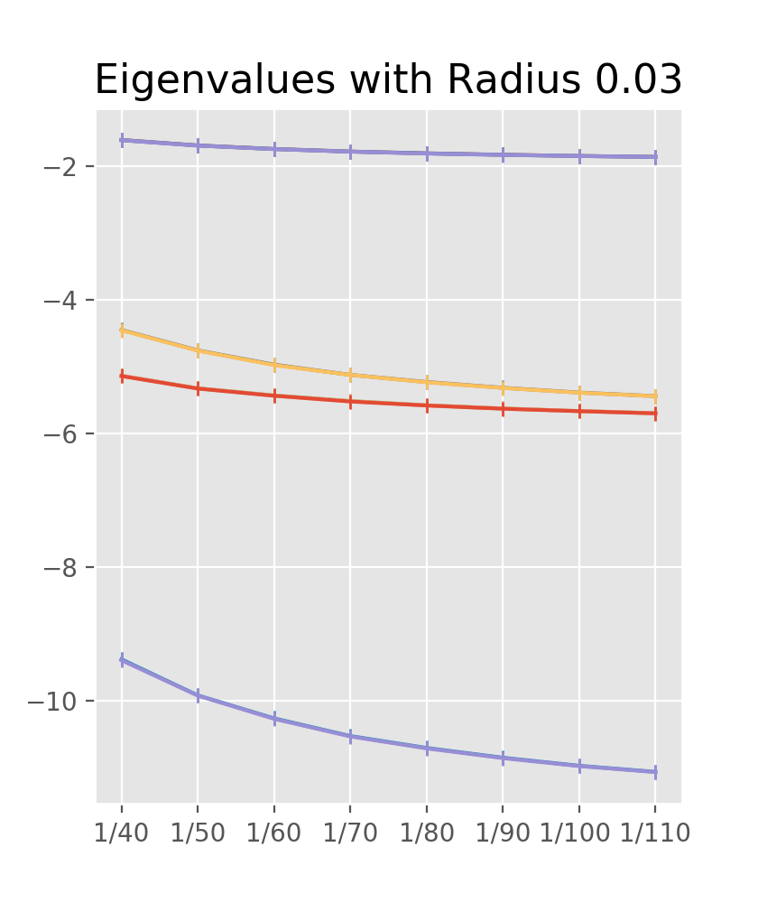
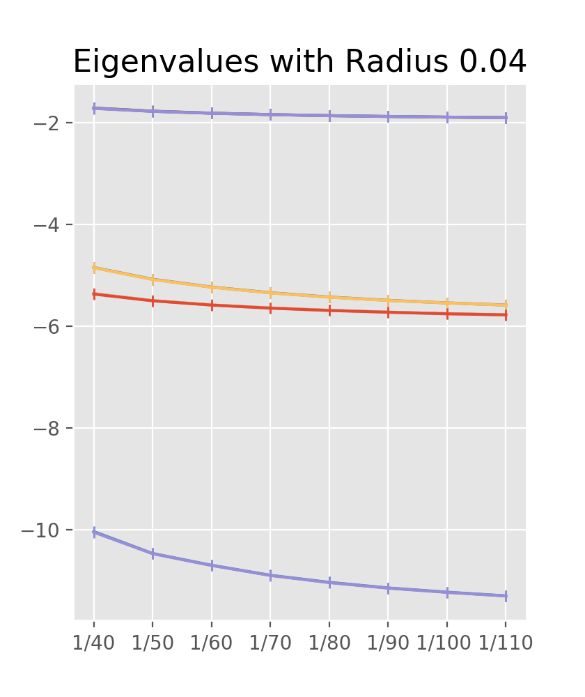
Table S1 reports the first ten non-zero surface eigenvalues on $S^{2}$ (counting multiplicity) by Algorithm 2 over grid size ${1\over n}$ for $n=40$ to 110 over shell thickness $r=0.02$ to 0.05 over $S^{2}$, which is the $\epsilon$-neighborhood of the grid. According to Table S1, we see that as the shell becomes thinner (smaller $y$ value) and the grid becomes finer (bigger $x$ value), the eigenvalues of the discrete $S^{2}$ converge to the true eigenvalues on a sphere, as discussed in Section 2.1. The multiplicity of eigenvalues $-\ell(\ell+1)$ is $2\ell+1$ for $\ell=1,2,3$, as expected.

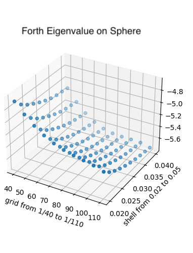
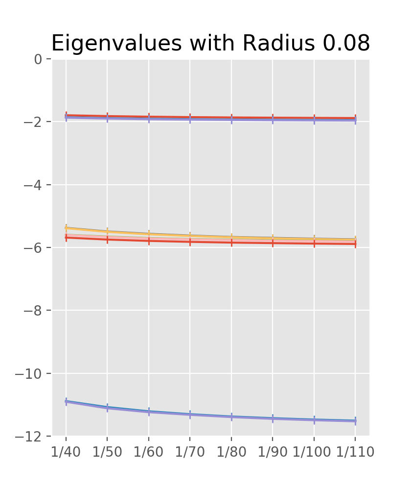
Table S2 reports the first ten non-zero surface eigenvalues by Algorithm 3 over grid size ${1\over n}$ for $n=40$ to 110 over shell thickness $r=0.05$ to 0.08 over $S^{2}$. Similar trends are found between Table S1 and Table S2. The results suggest that as the thickness of a surface and the length of the cubes approach zero, the computed discrete eigenvalues approximate the smooth eigenvalue more accurately.

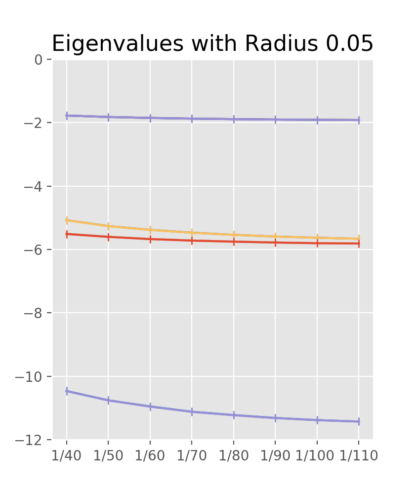
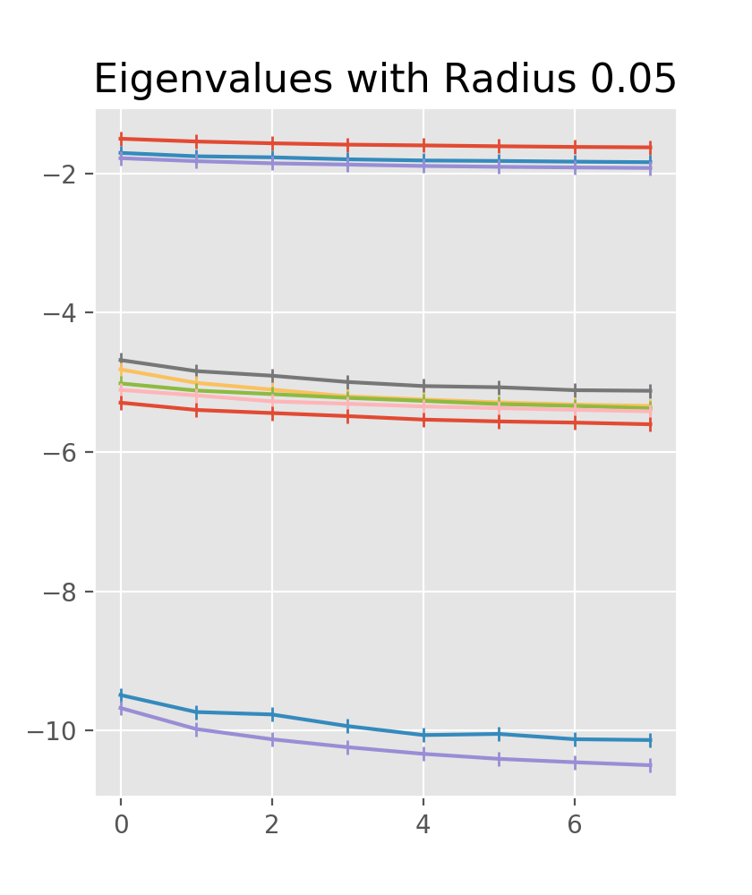
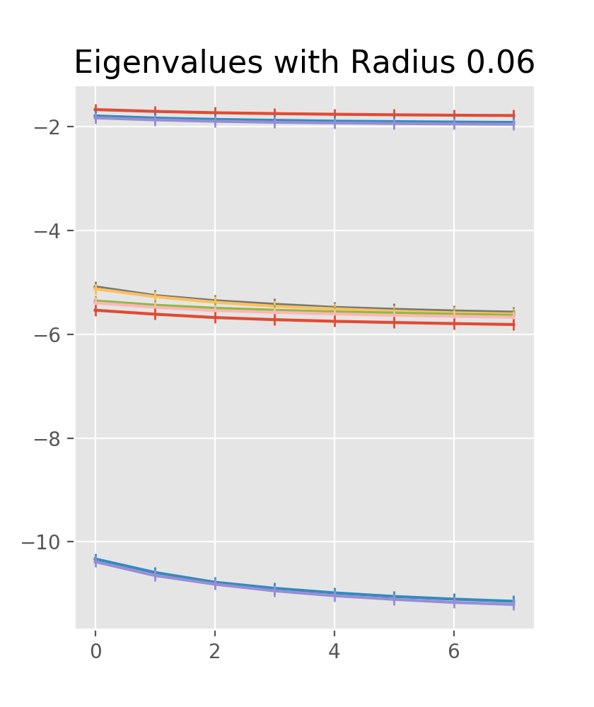
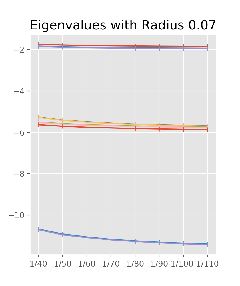
Fig. 3 and Fig. 4 exhibit computed surface eigenvalues by Algorithm 2 and Algorithm 3, respectively. Fig. 5 displays the change of eigenvalues as the radius increases with Algorithm 2 (first row) and Algorithm 3 (second row). The $x$-axis indicates the length of the lattice interval, and the $y$-axis indicates the computed eigenvalues. As the shell becomes thicker, the eigenvalues on the grid converge to eigenvalues on the smooth $S^{2}$ sooner. Fig. A3 and Fig. A4 display values of eigenvectors on $S^{2}$.

Figure 3: The first 3 non-zero eigenvalues (excluding multiplicity) on $S^{2}$ represented as a triangle mesh in 3D. Left: The first eigenvalue $-\ell(\ell+1)=-2$ on $S^{2}$. Middle: The second eigenvalue $-\ell(\ell+1)=-6$ on $S^{2}$ with multiplicity $2\ell+1$ for $\ell=2$. Right: The third eigenvalue $-\ell(\ell+1)=-12$ on $S^{2}$ with multiplicity $2\ell+1$ for $\ell=3$.

Figure 4: The first ten non-zero eigenvalues and multiplicity on $S^{2}$ represented as a point cloud in 3D. Left: The first eigenvalue $-\ell(\ell+1)=-2$ on $S^{2}$. Middle: The second eigenvalue $-\ell(\ell+1)=-6$ on $S^{2}$ with multiplicity $2\ell+1$ for $\ell=2$. Right: The third eigenvalue $-\ell(\ell+1)=-12$ on $S^{2}$ with multiplicity $2\ell+1$ for $\ell=3$.

Figure 5: Change of the first ten eigenvalues on $S^{2}$ represented as a point cloud as the shell radius increases with Algorithm 2 (first row) and Algorithm 3 (second row).

4.2 Ellipsoids and Urakawa’s Validation on Yau’s Conjecture

In this section, we report numerical experiments on the ten non-zero eigenvalues for five different ellipsoids using Algorithm 3. Table 1 reports the first ten non-zero surface eigenvalues on specified ellipsoids. In the table, CPU time measures the number of clock cycles summed across all threads that the Matlab process has used since Matlab started; the units are in seconds. All computations are performed on 170 GB memory allocation with 64 cores.

In Jumonji and Urakawa’s work on the eigenvalue problems of the Laplacian for bounded domains and embedded compact surfaces in the 3-dimensional Euclidean space [10], they examined Yau’s conjecture on the eigenvalues between embedded surfaces and their enclosed 3-dimensional bounded domains [26]. In Jumonji and Urakawa’s paper, they reported the first non-zero Laplacian eigenvalues of the ellipsoid with $a,b,c=1,3,3$ are 0.3, 0.3, 0.4, 0.8, 0.8, 1.2, and 1.2, agreeing with our computation result, displayed in Table 1 in the fifth column.

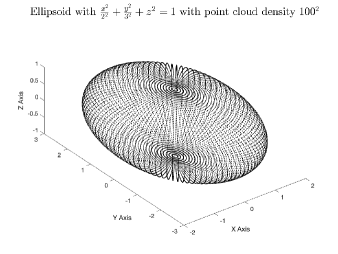
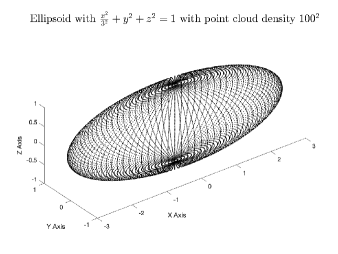
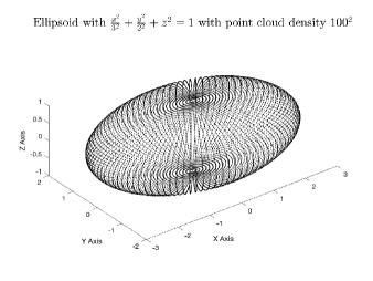
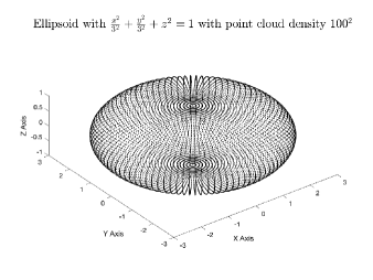
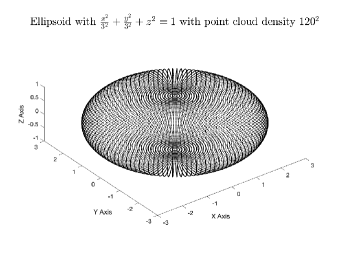
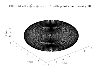
Fig. 6 exhibits the point cloud of ellipsoids $\displaystyle{x^{2}\over 2^{2}}+{y^{2}\over 3^{2}}+z^{2}=1$, $\displaystyle{x^{2}\over 3^{2}}+y^{2}+z^{2}=1$, $\displaystyle{x^{2}\over 3^{2}}+{y^{2}\over 2^{2}}+z^{2}=1$, and $\displaystyle{x^{2}\over 3^{2}}+{y^{2}\over 3^{2}}+z^{2}=1$, respectively, with point density $100^{2}$, and the point cloud of the ellipsoid $\displaystyle{x^{2}\over 3^{2}}+{y^{2}\over 3^{2}}+z^{2}=1$ with point density $120^{2}$ and $200^{2}$. Here the point cloud density refers to the number of points in the point cloud that form the ellipsoid. In particular, the eigenvalues of the ellipsoid $\displaystyle{x^{2}\over 2^{2}}+{y^{2}\over 3^{2}}+z^{2}=1$ should be the same as those of the ellipsoid $\displaystyle{x^{2}\over 3^{2}}+{y^{2}\over 2^{2}}+z^{2}=1$, since the latter is just an $SO(3)$ rotation of the first one, which can be observed accordingly from Table 1.

Figure 6: Point cloud of ellipsoids. 1: The point cloud of the ellipsoid $\displaystyle{x^{2}\over 2^{2}}+{y^{2}\over 3^{2}}+z^{2}=1$ with point density $100^{2}$. 2: The point cloud of the ellipsoid $\displaystyle{x^{2}\over 3^{2}}+y^{2}+z^{2}=1$ with point density $100^{2}$. 3: The point cloud of the ellipsoid $\displaystyle{x^{2}\over 3^{2}}+{y^{2}\over 2^{2}}+z^{2}=1$ with point density $100^{2}$. 4: The point cloud of the ellipsoid $\displaystyle{x^{2}\over 3^{2}}+{y^{2}\over 3^{2}}+z^{2}=1$ with point density $100^{2}$. 5: The point cloud of the ellipsoid $\displaystyle{x^{2}\over 3^{2}}+{y^{2}\over 3^{2}}+z^{2}=1$ with point density $120^{2}$. 6: The point cloud of the ellipsoid $\displaystyle{x^{2}\over 3^{2}}+{y^{2}\over 3^{2}}+z^{2}=1$ with point density $200^{2}$.

Table 1: The first ten non-zero surface eigenvalues by the meshless algorithm with $r=0.11$ and $n=50$ on 64 Cores and 170GB Memory HPC.

	$\displaystyle{x\over 2^{2}}+{y\over 3^{2}}+z^{2}=1$	$\displaystyle{x^{2}\over 3^{2}}+y^{2}+z^{2}=1$	$\displaystyle{x^{2}\over 3^{2}}+{y^{2}\over 2^{2}}+z^{2}=1$	$\displaystyle{x^{2}\over 3^{2}}+{y^{2}\over 3^{2}}+z^{2}=1$	$\displaystyle{x^{2}\over 3^{2}}+{y^{2}\over 2}+z^{2}=1$
Eigenvalues	-0.315241	-0.253582	-0.315241	-0.308855	-0.3228
	-0.596258	-1.126602	-0.596258	-0.308855	-0.9139
	-0.662100	-1.230701	-0.662100	-0.457628	-0.9425
	-1.017389	-1.363820	-1.017389	-0.833177	-1.0820
	-1.243444	-2.203574	-1.243444	-0.833941	-1.7189
	-1.486521	-2.276262	-1.486521	-1.219271	-1.8059
	-2.045236	-2.336757	-2.045236	-1.219271	-2.2293
	-2.048874	-3.549628	-2.048874	-1.269028	-2.8636
	-2.060981	-3.584377	-2.060981	-1.562024	-3.0742
	-2.216862	-3.975534	-2.216862	-1.562024	-3.1174
Elapsed Time	736”	425”	795”	1,341”	639”
CPU Time	5,043”	2,413”	5,440”	7,770”	4,057”

Table 2 compares the surface eigenvalues of the ellipsoid $\displaystyle{x^{2}\over 3^{2}}+{y^{2}\over 3^{2}}+z^{2}=1$ with various point cloud densities. Comparing to results reported in Jumonji and Urakawa, both the point cloud density and meshless algorithm parameters contribute to the convergence of eigenvalues. More specifically, greater point cloud density, thicker grid (greater shell thickness $r$), and denser grid (greater $n$) all lead to a more precise eigenvalue.

Table 2: The first ten non-zero surface eigenvalues by the meshless algorithm with 64 Cores and 170GB Memory with point cloud density $100^{2}$, $120^{2}$, $200^{2}$, $500^{2}$, and $1000^{2}$.

$\displaystyle{x^{2}\over 3^{2}}+{y^{2}\over 3^{2}}+z^{2}=1$
	Point Cloud Density $100^{2}$			Point Cloud Density $120^{2}$		Point Cloud Density $200^{2}$
	$r=0.05$	$r=0.05$	$r=0.05$	$r=0.05$	$r=0.05$	$r=0.05$	$r=0.05$
	$n=50$	$n=75$	$n=100$	$n=50$	$n=75$	$n=50$	$n=75$
Eigenvalues	-0.173892	-0.178447	-0.180789	-0.299862	-0.303826	-0.299862	-0.303826
	-0.173892	-0.178568	-0.180789	-0.299862	-0.303885	-0.299862	-0.303885
	-0.263055	-0.273016	-0.276887	-0.415050	-0.434217	-0.415050	-0.434217
	-0.265516	-0.273873	-0.277627	-0.793171	-0.806634	-0.793171	-0.806634
	-0.284125	-0.301827	-0.312457	-0.795942	-0.807992	-0.795942	-0.807992
	-0.318465	-0.331424	-0.336788	-1.145733	-1.177993	-1.145733	-1.177993
	-0.318465	-0.332699	-0.336788	-1.145733	-1.178085	-1.145733	-1.178085
	-0.347359	-0.368679	-0.374133	-1.193512	-1.238377	-1.193512	-1.238377
	-0.365683	-0.376422	-0.381585	-1.471670	-1.496612	-1.471670	-1.496612
	-0.383497	-0.399842	-0.407944	-1.471670	-1.497865	-1.471670	-1.497865
Elapsed Time	63”	305”	1,262”	173”	1,137”	173”	1,116”
CPU Time	249”	1,183”	4,210”	949”	7,255”	938”	7,538”
	Point Cloud Density $500^{2}$			Point Cloud Density $1000^{2}$			$500^{2}$	$1000^{2}$
	$r=0.05$	$r=0.05$	$r=0.05$	$r=0.05$	$r=0.05$	$r=0.05$	$r=0.08$	$r=0.08$
	$n=50$	$n=75$	$n=100$	$n=50$	$n=75$	$n=100$	$n=50$	$n=50$
Eigenvalues	-0.303699	-0.308881	-0.311363	-0.302948	-0.308269	-0.310890	-0.309011	-0.308697
	-0.303699	-0.308910	-0.311363	-0.302948	-0.308324	-0.310890	-0.309011	-0.308697
	-0.447712	-0.466251	-0.475603	-0.451377	-0.469358	-0.478537	-0.471729	-0.472977
	-0.822690	-0.844795	-0.855671	-0.821883	-0.844126	-0.855192	-0.846485	-0.845983
	-0.846778	-0.860377	-0.866436	-0.847143	-0.861282	-0.867818	-0.862488	-0.862434
	-1.201132	-1.233425	-1.249930	-1.205294	-1.237182	-1.253610	-1.242967	-1.244217
	-1.201132	-1.233541	-1.249930	-1.205294	-1.237580	-1.253610	-1.242967	-1.244217
	-1.204181	-1.245586	-1.265774	-1.206545	-1.246583	-1.266857	-1.250757	-1.251632
	-1.582467	-1.619629	-1.637757	-1.583844	-1.621378	-1.640358	-1.625266	-1.625361
	-1.582467	-1.620202	-1.637757	-1.583844	-1.622490	-1.640358	-1.625266	-1.625361
Elapsed Time	258”	1,516”	7,894”	290”	1,885”	8,239”	705”	898”
CPU Time	1,346”	9,588”	59,145”	1,331”	11,290”	59,262”	4,390”	4,760”

4.2.1 Tetrahedron

We present the Laplacian eigenvalues of a 3-sided tetrahedron and a 4-sided tetrahedron, shown in Fig. A1. The results are displayed in Table 3, where Surface column indicates eigenvalues computed by the classical algorithm for triangle mesh by Reuter [17], the Mesh Vertex column represents the eigenvalues computed by meshless algorithm using the point cloud consists of the vertex set from a triangle mesh, and the Point Cloud column represent eigenvalues computed by meshless algorithm (Algorithm 3) using a generated point cloud of respective surface. A discussion about the analytic solution to a tetrahedron could be found in [6].

Table 3: The first ten non-zero surface eigenvalues of the 3-sided regular tetrahedron and 4-sided regular tetrahedron by triangle surface algorithm and the meshless algorithm with point cloud density $100^{2}$ and shell thickness 0.05.

	3-sided Regular Tetrahedron			4-sided Regular Tetrahedron
	Surface	Meshless algorithm		Surface	Meshless algorithm
		Point Cloud	Mesh Vertex		Original	Mesh Vertex
Eigenvalues	-3.6214	-3.3574	-3.3450	-4.3830	-4.0153	-4.2557
	-3.6214	-3.4153	-3.3782	-4.3830	-4.2599	-4.3071
	-5.8424	-4.8823	-5.2485	-4.3830	-4.3330	-4.3378
	-11.1263	-10.5358	-10.4637	-13.1278	-12.8418	-13.2930
	-11.1263	-10.6727	-10.5752	-13.1278	-13.1429	-13.3975
	-17.4897	-15.0514	-15.6586	-13.1278	-13.2677	-13.5373
	-18.1964	-16.3376	-16.9002	-17.4897	-16.2846	-16.5812
	-18.1964	-16.5558	-17.0233	-17.4897	-17.0448	-17.4354
	-23.2946	-20.1906	-20.9053	-17.4897	-17.1762	-17.5524
	-23.7987	-23.5115	-23.2507	-17.4897	-30.5332	-30.2258
Elapsed Time	0.84”	157”	118”	0.72”	249”	217”
CPU Time	7.88”	878”	624”	14”	1,445”	1,071”

4.2.2 Cube

We present eigenvalues of a cube with vertices at $(\pm 1,\pm 1,\pm 1)$. The computed eigenvalues are presented in Table 4. The triangle mesh used for the cube is displayed in Fig. A2 on the left, and we also used a separate point cloud surface of the cube. In Table 4, the forth column, Mesh Vertex, represents the eigenvalues computed by meshless algorithm (Algorithm 3) using the point cloud consists of the vertex set from a triangle mesh. The first three columns are computed eigenvalues of a cube represented by a generated point cloud.

Table 4: The first ten non-zero surface eigenvalues of a cube with vertices at $(\pm 1,\pm 1,\pm 1)$ by the meshless algorithm with point cloud density $100^{2}$ and shell thickness 0.05.

	30 points on each edge	50 points on each edge	Mesh Vertex	Surface
Eigenvalues	-0.9416	-1.0571	-0.9781	-1.0412
	-0.9416	-1.0571	-0.9781	-1.0412
	-0.9417	-1.0571	-0.9781	-1.0412
	-2.5737	-2.8859	-2.6651	-2.8728
	-2.5737	-2.8859	-2.6651	-2.8728
	-2.5737	-2.8859	-2.6651	-2.8728
	-3.2527	-3.6592	-3.3990	-3.5307
	-3.2528	-3.6592	-3.3990	-3.5307
	-4.4080	-4.9393	-4.5610	-4.9308
	-5.8522	-6.5749	-6.0938	-6.4163
Elapsed Time	1,066”	1,768”	1,492”	0.79”
CPU Time	6,320”	10,987”	8,036”	740”

4.2.3 Cone

In this section, we report the computed eigenvalues using the classical surface algorithm and meshless algorithm (Algorithm 3); the results are reported in Table 5, where the first three columns report eigenvalues computed by the meshless algorithm, and the last column reports eigenvalues computed by the surface algorithm. In particular, the first two columns report eigenvalues computed by meshless algorithm using generated point cloud, and the third column reports eigenvalues computed by meshless algorithm using the point cloud extracted from the triangle mesh, as exhibited in Fig. A2 on the right. We also display values of eigenvectors on this cone in Fig. A5 and Fig. A6.

Table 5: The first ten non-zero surface eigenvalues of a cone with vertex at the origin and base at $z=1$ with radius = 1 by the meshless algorithm with point cloud density $100^{2}$ and shell thickness 0.05.

	20 points on each edge	50 points on each edge	Mesh Vertex	Surface
Eigenvalues	-1.3725	-2.3616	-3.0001	-3.0376
	-2.8905	-3.2116	-3.0001	-3.0377
	-3.0874	-3.9597	-4.1453	-3.8591
	-5.6597	-6.4916	-8.4367	-8.5843
	-5.7116	-8.6735	-8.5087	-8.5854
	-6.5111	-10.7776	-10.6293	-10.3370
	-7.2630	-11.1218	-12.3705	-11.4486
	-7.8935	-11.9478	-12.3705	-11.4491
	-10.0452	-13.4958	-16.2407	-16.4751
	-10.3218	-14.0009	-16.2407	-16.4761
Elapsed Time	147”	324”	380”	2.02”
CPU Time	705”	1,815”	2,006”	2,049”

4.3 Computed First Ten Non-zero Eigenvalues of Genus 1 Surface

Table 6 reports the first ten non-zero surface eigenvalues by the meshless algorithm of a genus 1 surface.

Table 6: The first ten non-zero surface eigenvalues by the meshless algorithm with 64 Cores and 170GB.

	$r=0.05$	$r=0.05$	$r=0.08$	$r=0.08$	$r=0.11$
	$n=75$	$n=100$	$n=75$	$n=75$	$n=100$
Eigenvalues	-0.617180	-0.628299	-0.646848	-0.653546	-0.672847
	-2.079415	-2.112728	-2.152381	-2.173507	-2.200838
	-2.494772	-2.533026	-2.582687	-2.606614	-2.640699
	-3.088792	-3.136877	-3.198115	-3.227173	-3.273606
	-3.391403	-3.436752	-3.511123	-3.544625	-3.605186
	-4.661078	-4.721061	-4.821988	-4.861155	-4.933898
	-5.473066	-5.574882	-5.698128	-5.751677	-5.834958
	-6.534291	-6.644320	-6.756330	-6.824672	-6.883822
	-6.632011	-6.733570	-6.904994	-6.969889	-7.129169
	-7.239121	-7.338298	-7.541480	-7.603741	-7.796873
Elapse Time	216”	882”	686”	3,241”	1,421”
CPU Time	1,166”	5,743”	4,543”	23,234”	9,871”

4.4 Computed First Ten Non-zero Eigenvalues of Genus 2 Surface

Table 7 reports the first ten non-zero surface eigenvalues by the meshless algorithm of a genus 2 surface.

Table 7: The first ten non-zero surface eigenvalues by the meshless algorithm with 64 Cores and 170GB.

	$r=0.05$	$r=0.05$	$r=0.08$
	$n=75$	$n=100$	$n=75$
Eigenvalues	-0.750970	-0.764963	-0.907334
	-0.955846	-0.973025	-1.124415
	-1.167671	-1.182242	-1.628818
	-1.419964	-1.429386	-1.667057
	-1.990223	-2.017348	-2.518728
	-2.292042	-2.315880	-2.733560
	-2.352482	-2.393655	-2.819258
	-2.386239	-2.414864	-3.015961
	-2.786546	-2.824579	-3.486652
	-3.308398	-3.375575	-4.203104
Elapse Time	199”	626”	1,449”
CPU Time	1,041”	3,946”	11,563”

4.5 Face

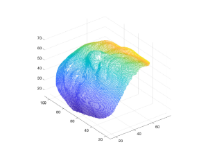
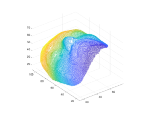
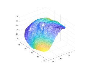
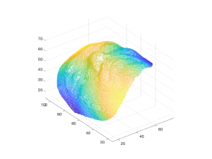
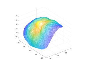
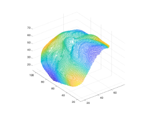
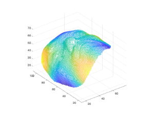
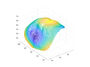
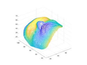
In this section, we report numerical results of the first ten non-zero surface eigenvalues using classical triangle mesh-based algorithm (Algorithm 1), a lattice that is approximated by triangle mesh surfaces (Algorithm 2), and a lattice that is approximated by point cloud (Algorithm 3), at different shell thickness and grid density in Table 8. We also display values of eigenvectors on the face in Fig. 7.

Table 8: The first ten non-zero surface eigenvalues by Algorithm 1, 2, and 3 at different shell thickness and grid density.

	Surface	Algorithm 2			Algorithm 3
		$r$ = 0.2	$r$ = 0.2	$r$ = 1	$r$ = 20	$r$ = 20	$r$ = 30
		$n$ = 3	$n$ = 5	$n$ = 3	$n$ = 0.05	$n$ = 0.5	$n$ = 0.5
Eigenvalues	-0.0003	-0.0002	-0.0002	-0.0003	-0.0002	-0.0002	-0.0002
	-0.0004	-0.0002	-0.0003	-0.0003	-0.0003	-0.0003	-0.0003
	-0.0009	-0.0005	-0.0007	-0.0008	-0.0005	-0.0007	-0.0006
	-0.0009	-0.0006	-0.0007	-0.0008	-0.0006	-0.0007	-0.0006
	-0.0011	-0.0007	-0.0009	-0.0011	-0.0008	-0.0009	-0.0008
	-0.0017	-0.0010	-0.0013	-0.0015	-0.0009	-0.0013	-0.0011
	-0.0018	-0.0011	-0.0014	-0.0017	-0.0011	-0.0014	-0.0013
	-0.0023	-0.0014	-0.0019	-0.0022	-0.0013	-0.0019	-0.0016
	-0.0026	-0.0015	-0.0020	-0.0024	-0.0015	-0.0020	-0.0017
	-0.0027	-0.0017	-0.0021	-0.0025	-0.0016	-0.0021	-0.0018

Figure 7: Eigenfunctions on the face.

5 Comparison with Analytic Solutions

This section presents a comparison of the analytic solution and numerical solution of the first ten non-zero Laplacian eigenvalues of $S^{2}$ and a cone.

5.1 Comparison with Analytic Solution on $S^{2}$

This section compares our meshless algorithm and Reuter’s surface algorithm for Laplacian eigenvalues on $S^{2}$ with the analytic solution. The results are reported in Table 9.

Table 9: Comparison of the first ten non-zero surface Laplacian eigenvalues on $S^{2}$ computed by the meshless algorithm and surface algorithm with the analytic solution.

	Meshless Algorithm					Surface	Analytic
	$n=70$	$n=80$	$n=90$	$n=100$	$n=110$
$r=0.08$	-1.855325	-1.86539	-1.873125	-1.879448	-1.884542	-1.9984	-2
	-1.921102	-1.931773	-1.938983	-1.945495	-1.950469	-2.0005	-2
	-1.935166	-1.94506	-1.953552	-1.959711	-1.965312	-2.0010	-2
	-5.62263	-5.667128	-5.696293	-5.722359	-5.74309	-5.9924	-6
	-5.634138	-5.6763	-5.709371	-5.733887	-5.754284	-5.9944	-6
	-5.734904	-5.754076	-5.772994	-5.788926	-5.801214	-5.9944	-6
	-5.742877	-5.765704	-5.784355	-5.797827	-5.81031	-5.9966	-6
	-5.821731	-5.845335	-5.862249	-5.877002	-5.889156	-5.9977	-6
	-11.302968	-11.376339	-11.429968	-11.473721	-11.507684	-11.9628	-12
	-11.323203	-11.395242	-11.451686	-11.494617	-11.529418	-11.9690	-12

5.2 Comparison with Analytic Solution on a Cone

The analytic solutions of surface Laplacian eigenvalues on the cone surface are reported in Table 10, and the comparison with numerical values is reported in Table 11.

Table 10: Analytic surface Laplacian eigenvalues on a cone with $n$ from 0 to 9.

	Analytic Surface Laplacian Eigenvalues $<10.1^{2}$ from Bessel function $J_{n}$
$n$ = 0	0	3.85927	10.3388	20.4572	34.3839	50.7012	71.6951	94.8567
$n$ = 1	0	3.03793	11.4536	21.9914	36.2099	54.2471	74.6358	99.7367
$n$ = 2	0	8.58743	21.7955	36.451	54.8071	76.9932	101.448
$n$ = 3	0	16.485	34.7316	53.6064	76.1614
$n$ = 4	0	26.6572	50.1688	73.372	100.197
$n$ = 5	0	39.0603	68.0441	95.684
$n$ = 6	0	53.665	88.3116
$n$ = 7	0	70.4497
$n$ = 8	0	89.398
$n$ = 9	0

Table 11: Analytic surface Laplacian eigenvalues on a cone with multiplicity with $n$ from 0 to 9 and numerical surface Laplacian eigenvalues by the standard surface algorithm.

	Numerical Eigenvalues	Analytic Eigenvalues	Bessel $J_{n}$
Eigenvalues	0	0	0
	-3.0376	-3.03793	1
	-3.0377	-3.03793	1
	-3.8591	-3.85927	0
	-8.5843	-8.58743	2
	-8.5854	-8.58743	2
	-10.3370	-10.3388	0
	-11.4486	-11.4536	1
	-11.4491	-11.4536	1
	-16.4751	-16.485	3
	-16.4761	-16.485	3
	-20.4440	-20.4572	0
	-21.7744	-21.7955	2
	-21.7831	-21.7955	2
	-21.9765	-21.9914	1
	-21.9777	-21.9914	1
	-26.6327	-26.6572	4
	-26.6335	-26.6572	4
	-34.3505	-34.3839	0
	-34.6892	-34.7316	3
	-34.6906	-34.7316	3
	-36.1593	-36.2099	1
	-36.1622	-36.2099	1
	-36.4016	-36.451	2
	-36.4194	-36.451	2
	-39.0084	-39.0603	5
	-39.0105	-39.0603	5
	-50.0815	-50.1688	4
	-50.0843	-50.1688	4
	-50.6146	-50.7012	0

6 Supplementary Material

Table S1 reports the effect of shell thickness and grid density using Algorithm 2. We observe that denser grids (i.e., greater $n$) lead to an eigenvalue closer to the analytic solution. We also observe that thicker shells lead to eigenvalues better converging to the true value. Table S2 reports analogous results for Algorithm 3.

Table S1: The first ten non-zero surface eigenvalues by Algorithm 2.

	$n=40$	$n=50$	$n=60$	$n=70$	$n=80$	$n=90$	$n=100$	$n=110$
	-1.3898	-1.5193	-1.6106	-1.6687	-1.7121	-1.7458	-1.7721	-1.7938
	-1.3919	-1.5239	-1.6116	-1.6696	-1.7142	-1.7468	-1.7736	-1.7943
	-1.3964	-1.5254	-1.6162	-1.6704	-1.7149	-1.7473	-1.7743	-1.7950
	-3.6430	-4.1117	-4.457	-4.672	-4.8446	-4.9748	-5.0746	-5.1621
	-3.6478	-4.1221	-4.4638	-4.6746	-4.8487	-4.9766	-5.0796	-5.1637
	-4.6407	-4.936	-5.1297	-5.2616	-5.3604	-5.4318	-5.4968	-5.5394
	-4.646	-4.9382	-5.1336	-5.2632	-5.3617	-5.4357	-5.4972	-5.5431
	-4.6554	-4.9452	-5.1414	-5.2713	-5.3642	-5.4379	-5.4988	-5.5447
	-7.9641	-8.7511	-9.3728	-9.7605	-10.0492	-10.2665	-10.4386	-10.5886
$r=0.02$	-7.9974	-8.7645	-9.3854	-9.7646	-10.0651	-10.2735	-10.4463	-10.5923
	-1.6109	-1.6928	-1.7454	-1.7835	-1.8106	-1.8321	-1.8501	-1.8638
	-1.613	-1.6938	-1.7466	-1.7847	-1.8115	-1.8334	-1.8508	-1.8647
	-1.6144	-1.696	-1.7481	-1.7855	-1.8141	-1.8347	-1.8515	-1.8649
	-4.4528	-4.7585	-4.9719	-5.1243	-5.2314	-5.3178	-5.3894	-5.4423
	-4.4577	-4.7624	-4.9789	-5.1253	-5.2358	-5.3209	-5.3919	-5.4439
	-5.1364	-5.3247	-5.4322	-5.5158	-5.5795	-5.6271	-5.6656	-5.6978
	-5.1381	-5.3262	-5.4361	-5.5205	-5.5821	-5.6278	-5.6663	-5.6989
	-5.1424	-5.3299	-5.4372	-5.523	-5.583	-5.6316	-5.6679	-5.7003
	-9.3796	-9.9188	-10.2626	-10.5272	-10.7054	-10.8514	-10.9721	-11.0632
$r=0.03$	-9.3941	-9.9223	-10.2703	-10.5338	-10.7124	-10.8581	-10.9768	-11.0664
	-1.7103	-1.7708	-1.8104	-1.8386	-1.8592	-1.875	-1.8885	-1.8983
	-1.7129	-1.7748	-1.8115	-1.8393	-1.8599	-1.8759	-1.8887	-1.8987
	-1.718	-1.7754	-1.8127	-1.84	-1.8605	-1.8765	-1.889	-1.8995
	-4.8447	-5.0757	-5.2287	-5.3407	-5.4249	-5.4896	-5.54	-5.5824
	-4.8491	-5.0809	-5.2322	-5.3446	-5.4287	-5.4924	-5.541	-5.5849
	-5.356	-5.4945	-5.5798	-5.6394	-5.6848	-5.7214	-5.7524	-5.7731
	-5.3578	-5.4987	-5.58	-5.6425	-5.6867	-5.7224	-5.7533	-5.7749
	-5.3669	-5.499	-5.5827	-5.6437	-5.6891	-5.724	-5.7546	-5.775
	-10.0345	-10.4651	-10.6959	-10.8932	-11.0322	-11.142	-11.2248	-11.2982
$r=0.04$	-10.0471	-10.4685	-10.7004	-10.8968	-11.0383	-11.1465	-11.2298	-11.2995
	-1.7746	-1.8192	-1.8496	-1.8721	-1.8879	-1.8997	-1.9102	-1.9171
	-1.7756	-1.8201	-1.8507	-1.8723	-1.8883	-1.9012	-1.9109	-1.9171
	-1.7757	-1.8208	-1.8509	-1.8729	-1.8887	-1.9018	-1.9111	-1.9171
	-5.0739	-5.2616	-5.3801	-5.4703	-5.5379	-5.5912	-5.6303	-5.6629
	-5.0762	-5.2638	-5.3831	-5.4734	-5.5393	-5.5923	-5.6323	-5.6629
	-5.5049	-5.5981	-5.6691	-5.7163	-5.7516	-5.7772	-5.8006	-5.8117
	-5.5091	-5.6009	-5.6705	-5.7197	-5.7531	-5.7784	-5.8008	-5.8117
	-5.5113	-5.6028	-5.6724	-5.7206	-5.7532	-5.7819	-5.8024	-5.8117
	-10.4649	-10.7581	-10.9514	-11.1185	-11.2235	-11.3155	-11.3823	-11.4291
$r=0.05$	-10.4673	-10.7602	-10.9582	-11.1215	-11.2279	-11.3193	-11.3841	-11.4291

Table S2: The first ten non-zero surface eigenvalues by Algorithm 3.

	$n=40$	$n=50$	$n=60$	$n=70$	$n=80$	$n=90$	$n=100$	$n=110$
	-1.5006	-1.5406	-1.566	-1.5855	-1.5964	-1.6086	-1.6183	-1.6245
	-1.7041	-1.7527	-1.7678	-1.796	-1.813	-1.8199	-1.8299	-1.8378
	-1.7799	-1.8225	-1.8538	-1.8717	-1.8915	-1.904	-1.9131	-1.9208
	-4.6797	-4.8379	-4.9042	-4.9942	-5.0529	-5.0702	-5.1122	-5.1206
	-4.8138	-5.007	-5.1032	-5.2002	-5.2459	-5.2876	-5.3188	-5.3379
	-5.0147	-5.1173	-5.1679	-5.2225	-5.2658	-5.3115	-5.3381	-5.373
	-5.108	-5.1869	-5.2726	-5.3071	-5.3454	-5.3699	-5.3941	-5.4153
	-5.2912	-5.3956	-5.4406	-5.4844	-5.5344	-5.5607	-5.5778	-5.6016
	-9.4901	-9.7345	-9.7695	-9.9365	-10.0651	-10.0491	-10.1249	-10.1367
$r=0.05$	-9.6765	-9.9786	-10.1256	-10.2391	-10.3352	-10.407	-10.4557	-10.4985
	-1.6725	-1.7074	-1.7334	-1.7496	-1.7626	-1.7728	-1.7807	-1.78681
	-1.7944	-1.836	-1.8611	-1.8795	-1.8949	-1.9041	-1.9131	-1.9199
	-1.8314	-1.8702	-1.8979	-1.9163	-1.929	-1.9404	-1.9488	-1.9563
	-5.0865	-5.2556	-5.3538	-5.4236	-5.4826	-5.5197	-5.5507	-5.5750
	-5.1252	-5.2767	-5.3836	-5.4605	-5.5112	-5.5547	-5.587	-5.6091
	-5.3581	-5.4403	-5.4983	-5.5376	-5.5692	-5.5929	-5.6156	-5.6355
	-5.3945	-5.4805	-5.5429	-5.5778	-5.6091	-5.6338	-5.6532	-5.6711
	-5.5367	-5.6137	-5.678	-5.7192	-5.7502	-5.7737	-5.7945	-5.8127
	-10.3279	-10.589	-10.7767	-10.8936	-10.9816	-11.0511	-11.1024	-11.1439
$r=0.06$	-10.3811	-10.6479	-10.8146	-10.9429	-11.0362	-11.1066	-11.1658	-11.2056
	-1.748184	-1.7823	-1.8033	-1.8190	-1.8295	-1.839443	-1.846358	-1.851796
	-1.837259	-1.870554	-1.8926	-1.9078	-1.9199	-1.9282	-1.9360	-1.9418
	-1.854534	-1.890521	-1.9123	-1.9277	-1.9404	-1.9492	-1.9565	-1.9628
	-5.2646	-5.4120	-5.4916	-5.5586	-5.6063	-5.6409	-5.6708	-5.6930
	-5.2797	-5.4197	-5.5066	-5.5717	-5.6160	-5.6553	-5.6812	-5.7052
	-5.50673	-5.5794	-5.6328	-5.6691	-5.6955	-5.7163	-5.7350	-5.7481
	-5.52381	-5.6030	-5.6544	-5.6849	-5.7128	-5.7325	-5.7498	-5.7639
	-5.6335	-5.7060	-5.7556	-5.7861	-5.8155	-5.8350	-5.8534	-5.8673
	-10.6751	-10.9116	-11.059	-11.1716	-11.2464	-11.3109	-11.3573	-11.3983
$r=0.07$	-10.6963	-10.951	-11.0844	-11.1932	-11.2686	-11.3339	-11.3842	-11.4229
	-1.7956	-1.8226	-1.8414	-1.8553	-1.86539	-1.8731	-1.8794	-1.8845
	-1.859861	-1.8890	-1.9066	-1.9211	-1.9317	-1.9389	-1.9454	-1.9504
	-1.873071	-1.9011	-1.9226	-1.9351	-1.9450	-1.9535	-1.9597	-1.9653
	-5.3766	-5.4920	-5.5669	-5.622	-5.6671	-5.6962	-5.7223	-5.7430
	-5.3863	-5.5041	-5.5800	-5.6341	-5.6763	-5.7093	-5.7338	-5.7542
	-5.597	-5.6549	-5.7025	-5.7349	-5.7540	-5.7729	-5.7889	-5.8012
	-5.6031	-5.666	-5.7120	-5.7428	-5.7657	-5.7843	-5.7978	-5.8103
	-5.6855	-5.748	-5.7910	-5.8217	-5.8453	-5.8622	-5.8770	-5.8891
	-10.8871	-11.0775	-11.2104	-11.3029	-11.3763	-11.4299	-11.4737	-11.5076
$r=0.08$	-10.9073	-11.1150	-11.2387	-11.3232	-11.3952	-11.4516	-11.4946	-11.5294

 

Appendix

Triangle Mesh of 3-sided and 4-sided Regular Tetrahedron

The triangle mesh of 3-sided and 4-sided regular tetrahedron we used for Reuter’s classical algorithm is displayed as Fig. A1.

Figure A1. Triangle mesh of 3-sided (left) and 4-sided (right) regular tetrahedron.

Cube and Cone

The point cloud and triangle mesh of a cube and a cone whose vertices are located at the origin and base at $z=1$ with radius = 1.

Figure A2. Triangle mesh of cube (left) and cone (right).

Figure A3. Eigenfunctions correspond to first 32 eigenvalues on a sphere.

Figure A4. Eigenfunctions correspond to the 33rd-64th eigenvalues on a sphere.

Figure A5. Eigenfunctions correspond to first 32 eigenvalues on a cone.

Figure A6. Eigenfunctions correspond to the 33rd-64th eigenvalues on a cone.

References

- 1. M. Belkin and P. Niyogi. Laplacian eigenmaps for dimensionality reduction and data representation. Neural computation, 15(6):1373–1396, 2003.
- 2. J. Brandman. A level-set method for computing the eigenvalues of elliptic operators defined on compact hypersurfaces. Journal of Scientific Computing, 37(3):282–315, 2008.
- 3. R. R. Coifman and S. Lafon. Diffusion maps. Applied and computational harmonic analysis, 21(1):5–30, 2006.
- 4. R. Courant and D. Hilbert. Methods of Mathematical Physics: Partial Differential Equations. John Wiley & Sons, 2008.
- 5. S. Dong, P.-T. Bremer, M. Garland, V. Pascucci, and J. C. Hart. Quadrangulating a mesh using Laplacian eigenvectors. Technical report, 2005.
- 6. E. Greif, D. Kaplan, R. S. Strichartz, and S. C. Wiese. Spectrum of the laplacian on regular polyhedra. arXiv preprint arXiv:1809.09909, 2018.
- 7. H. Hamidian, J. Hu, Z. Zhong, and J. Hua. Quantifying shape deformations by variation of geometric spectrum. In International Conference on Medical Image Computing and Computer-Assisted Intervention, pages 150–157. Springer, 2016.
- 8. H. Hamidian, Z. Zhong, F. Fotouhi, and J. Hua. Surface registration with eigenvalues and eigenvectors. IEEE transactions on visualization and computer graphics, 26(11):3327–3339, 2019.
- 9. J. Hu, H. Hamidian, Z. Zhong, and J. Hua. Visualizing shape deformations with variation of geometric spectrum. IEEE Transactions on Visualization and Computer Graphics, 23(1):721–730, 2016.
- 10. M. Jumonji and H. Urakawa. The eigenvalue problems for the Laplacian on compact embedded surfaces and three dimensional bounded domains. Interdisciplinary Information Sciences, 14(2):191–223, 2008.
- 11. A. Kovnatsky, M. M. Bronstein, A. M. Bronstein, K. Glashoff, and R. Kimmel. Coupled quasi-harmonic bases. In Computer Graphics Forum, volume 32, pages 439–448. Wiley Online Library, 2013.
- 12. B. Lévy. Laplace-beltrami eigenfunctions towards an algorithm that “understands” geometry. In IEEE International Conference on Shape Modeling and Applications 2006 (SMI’06), pages 13–13. IEEE, 2006.
- 13. O. Litany, E. Rodolà, A. M. Bronstein, and M. M. Bronstein. Fully spectral partial shape matching. In Computer Graphics Forum, volume 36, pages 247–258. Wiley Online Library, 2017.
- 14. C. B. Macdonald, J. Brandman, and S. J. Ruuth. Solving eigenvalue problems on curved surfaces using the closest point method. Journal of Computational Physics, 230(22):7944–7956, 2011.
- 15. M. Ovsjanikov, M. Ben-Chen, J. Solomon, A. Butscher, and L. Guibas. Functional maps: a flexible representation of maps between shapes. ACM Transactions on Graphics (ToG), 31(4):1–11, 2012.
- 16. M. Reuter. Hierarchical shape segmentation and registration via topological features of Laplace-Beltrami eigenfunctions. International Journal of Computer Vision, 89(2):287–308, 2010.
- 17. M. Reuter, S. Biasotti, D. Giorgi, G. Patanè, and M. Spagnuolo. Discrete Laplace-Beltrami operators for shape analysis and segmentation. Computers & Graphics, 33(3):381–390, 2009.
- 18. M. Reuter, F.-E. Wolter, and N. Peinecke. Laplace-spectra as fingerprints for shape matching. In Proceedings of the 2005 ACM symposium on Solid and physical modeling, pages 101–106, 2005.
- 19. M. Reuter, F.-E. Wolter, and N. Peinecke. Laplace-Beltrami spectra as ‘shape-DNA’ of surfaces and solids. Computer-Aided Design, 38(4):342–366, 2006.
- 20. E. Rodolà, L. Cosmo, M. M. Bronstein, A. Torsello, and D. Cremers. Partial functional correspondence. In Computer graphics forum, volume 36, pages 222–236. Wiley Online Library, 2017.
- 21. R. M. Rustamov. Laplace-Beltrami eigenfunctions for deformation invariant shape representation. In Proceedings of the fifth Eurographics symposium on Geometry processing, pages 225–233, 2007.
- 22. R. M. Rustamov, M. Ovsjanikov, O. Azencot, M. Ben-Chen, F. Chazal, and L. Guibas. Map-based exploration of intrinsic shape differences and variability. ACM Transactions on Graphics (TOG), 32(4):1–12, 2013.
- 23. S. Seo, M. K. Chung, and H. K. Vorperian. Heat kernel smoothing using Laplace-Beltrami eigenfunctions. In International Conference on Medical Image Computing and Computer-Assisted Intervention, pages 505–512. Springer, 2010.
- 24. Y. Shi, R. Lai, R. Gill, D. Pelletier, D. Mohr, N. Sicotte, and A. W. Toga. Conformal metric optimization on surface (CMOS) for deformation and mapping in Laplace-Beltrami embedding space. In International Conference on Medical Image Computing and Computer-Assisted Intervention, pages 327–334. Springer, 2011.
- 25. M. A. Shubin. Pseudodifferential operators and spectral theory, volume 200. Springer, 1987.
- 26. S.-T. Yau. Review of geometry and analysis. Asian Journal of Mathematics, 4(1):235–278, 2000.
- 27. W. Zeng, L. M. Lui, L. Shi, D. Wang, W. C. Chu, J. C. Cheng, J. Hua, S.-T. Yau, and X. Gu. Shape analysis of vestibular systems in adolescent idiopathic scoliosis using geodesic spectra. In International Conference on Medical Image Computing and Computer-Assisted Intervention, pages 538–546. Springer, 2010.