Functional Clustering of Neuronal Signals with FMM Mixture Models

Abstract

The identification of unlabelled neuronal electric signals is one of the most challenging open problems in neuroscience, widely known as Spike Sorting. Motivated to solve this problem, we propose a model-based approach within the mixture modeling framework for clustering oscillatory functional data called MixFMM. The core of the approach is the FMM waves, which are non-linear parametric time functions, flexible enough to describe different oscillatory patterns and simple enough to be estimated efficiently. In particular, specific model parameters describe the waveforms’ phase, amplitude, and shape. A mixture model is defined using FMM waves as basic functions and gaussian errors, and an EM algorithm is proposed for estimating the parameters. In addition, the approach includes a method for the number of clusters selection. Spike Sorting has received considerable attention in the literature, and different functional clustering approaches have traditionally been considered. We compare those approaches with the MixFMM in a broad collection of datasets, including benchmarking simulated and real data. The MixFMM approach achieves outstanding results in a selection of indexes across datasets, and the significant improvements attained in specific scenarios motivate interesting neuronal insights.

Keywords: Functional Data Analysis, Spike Sorting, Oscillatory Signals, Phase-Amplitude Variation

1 Introduction

The analysis of the electric activity of the neurons is regarded as one of the most practical and effective approaches to studying the nervous system. The electric signals recorded by electrodes register rapid voltage rises lasting a few milliseconds called spikes. The voltage returns to the initial baseline level in each spike, describing a single oscillation. The study of spikes is crucial in neuroscience, as spikes serve as the informational unit between neurons, and their firing rate and shape determine the cell’s morphological, functional, and genetic type. In particular, spikes fired by a particular neuron recorded under similar conditions, such as the electrode’s distance and orientation, are assumed to have a specific shape. Spike Sorting (SS) is the collection of techniques to identify spikes corresponding to different neurons. The correct identification of spikes is crucial for studying the connectivity patterns between close-by neurons [6], relating the firing of certain neurons to the memory process [33], the treatment of epileptic patients [42], or the development of high-accuracy brain-machine interfaces [25], among many other questions. However, SS remains one of the most challenging open problems in neuroscience. The main reasons are the low signal-to-noise ratio, the waveform variability of a particular neuron’s spikes, the selection of adequate features to characterize the spike shape, or the overlapping of spikes fired nearby in time. Algorithms that simultaneously address all of these issues are an ever-increasing necessity, as manual spike curation has become unaffordable in light of the increased data availability in the next generation of recording techniques [33].

The four traditional stages of SS are shown in Figure 1, top and bottom left. In stage 0, voltage traces are preprocessed, often with a basic bandpass filtering. Stage 1 entails the automatic spike detection and the signal segmentation into various sub-signals, each containing a single spike. Finally, stages 2 and 3 are devoted to the extraction of discriminant features and clustering, respectively. The focus of this paper is on stages 2 and 3, which may be quite different from one approach to another; features are mainly extracted using principal component analysis (PCA) or wavelet coefficients, while the most widely used clustering algorithms are k-means (KM) and Gaussian mixture models (GM). However, a complete list of alternative techniques used in stages 2 and 3 in SS is large. Some interesting references are [30, 14, 33, 8, 43, 32, 7, 44, 47, 45].

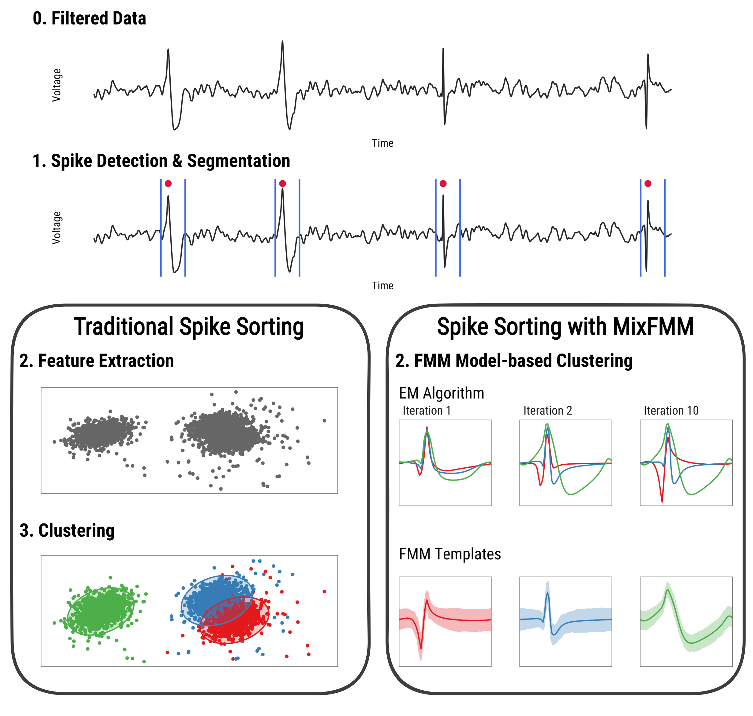
Figure 1: Overview of SS: stages 0 and 1 (top), stages 2 and 3 in traditional SS procedures (bottom left), and single model-based clustering stage in MixFMM model (bottom right).

We propose in this paper an original parametric model-based functional clustering approach as an alternative to stages 2 and 3 in traditional SS (Figure 1, bottom right).

Model-based functional clustering is an active topic in the literature [20, 17, 20, 21, 22, 50]. Different parametric models have been studied, mainly regression models and additive models defined by basic time functions such as splines, Fourier waves, or wavelets. The model choice depends on the available information, in terms of explicative variables, on the nature of the data, and on the sources of variation characterizing data, among other issues. For instance, Fourier methods might not be suitable for nonstationary signals. Specifically, two main sources of variation are considered in functional analysis, the amplitude variation that measures vertical variability, and the phase variation measuring horizontal (lateral) displacements [23, 26, 10]. Depending on the problem at hand, either both sources of variation are the focus or one is just nuisance and must be removed. Besides, some methods do not work adequately without prior correction for phase differences.

The model-based approach suitable for analyzing oscillatory signals that we present is the FMM mixture (MixFMM). The core is a mixture of gaussian distributions where the means are sums of FMM waves or components. FMM waves are non-linear time functions that describe a single oscillation with four parameters $(A,\alpha,\omega,\beta)$, which characterize the amplitude ($A$), phase ($\alpha$), and shape ($\beta,\omega$) of the waveform. In particular, the amplitude and phase source of variation issues can be easily handled using this model. Moreover, the mean cluster waveforms or templates can be compared in a simple way. Signals defined as combination of FMM waves have been successfully used to analyze oscillatory signals arising in different fields, such as ECG and gene expression data, as well as neuronal spikes [38, 37, 36, 35]. In all of these works, the method attains highly accurate predictions and allows the extraction of interpretable features, among other assets. The number of components is often associated with the prominent peaks and troughs in the signal, these being five for ECG signals or three for neuronal spikes. The first component, also called the dominant component, usually identifies the prominent underlying biological process and, in some contexts, explains most of the data variability, as in neuronal spikes. Finally, another remarkable property of FMM waves, very useful in functional analysis, is that they are truly dynamic that can be formulated as an ordinary differential equations system.

Noise existing in data is taken into account using FMM_m models, defined as signal plus error models where the signal is a combination of $m$ FMM waves and the error is assumed gaussian. The maximum likelihood estimator (MLE) of the parameters are derived using a backfitting algorithm, in which FMM₁ models are repeatedly fitted to the residue until a stop criterion is attained [40]. The novel approach is based on MixFMM_m models defined as an FMM_m mixture. We solve the MixFMM_m model’s parameter estimation with an expectation-maximization (EM) algorithm designed ad-hoc that makes use of the FMM_m estimation algorithm. In addition, we propose a likelihood-based method to select the number of clusters. The MixFMM approach has been validated in 10 benchmarking SS datasets (8 simulated and 2 real), including a wide variety of spike waveforms, noise levels, and recording situations. The results are compared with two standard approaches in SS, PCA plus either KM or GM, using indexes based on the associated groundtruth and internal cluster metrics. The MixFMM achieves outstanding results, clearly superior to its competitors in terms of accuracy, interpretability, robustness, cluster cohesion and separability. Moreover, the proposed method estimates the number of clusters better than other traditional approaches.

The rest of the paper is organized as follows. Section 2 introduces the MixFMM_m model, the estimation algorithm, and the number of clusters selection. Section 3 describes the datasets analyzed, and Section 4 presents the main results. Finally, in Section 5, concluding remarks and future work are discussed.

2 Methods

In the following, let us assume that $\boldsymbol{t}=(t_{1},...,t_{p})$, with $t_{0}\leq t_{1}<t_{2}<...<t_{p}\leq T$, and $\boldsymbol{x}_{1},...,\boldsymbol{x}_{n}$, $\boldsymbol{x}_{i}=(x_{i}(t_{1}),...,x_{i}(t_{p})),\forall i\in\{1,...,n\}$ are the time points and observed signals, also called curves. Without loss of generality, we assume that $t\in[0,2\pi)$. Otherwise, consider $t^{\prime}=\frac{(t-t_{0})2\pi}{T}$.

2.1 FMM background

An FMM wave is defined as follows,

$$W(t;A,\alpha,\beta,\omega)=A\cos\left(\beta+2\arctan\left(\omega\tan\left(\frac{t-\alpha}{2}\right)\right)\right).$$ (1)

Specifically, $A\in\Re^{+}$ and $\alpha\in[0,2\pi)$ are measures of the wave amplitude and phase location, respectively, while $\beta\in[0,2\pi)$ and $\omega\in[0,1]$ describe the shape. Figure 2 shows the waveform patterns for different parameter configurations.

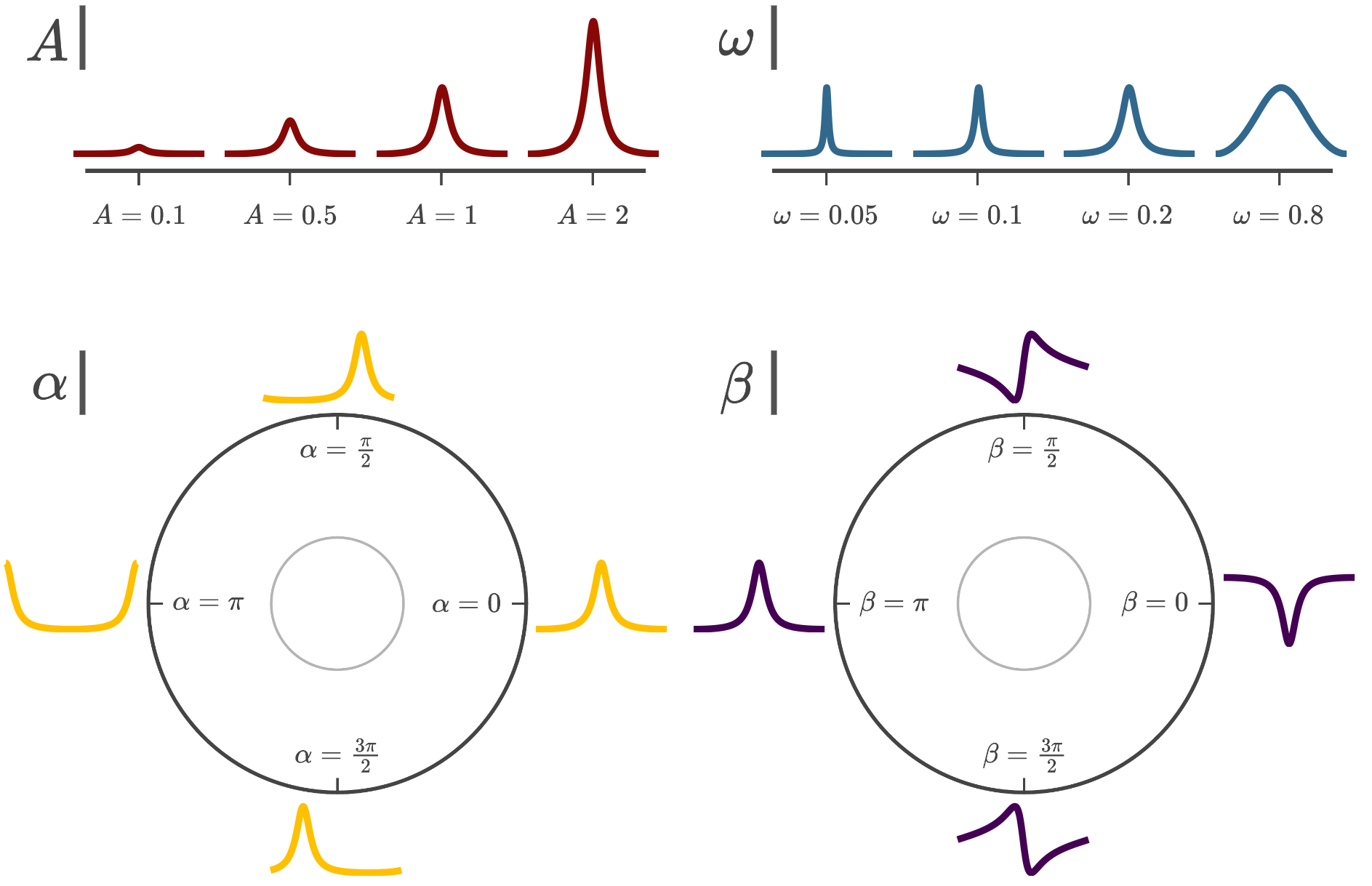
Figure 2: $W(t;A,\alpha,\beta,\omega)$ for various $(A,\alpha,\beta,\omega)$. Unless stated otherwise, $A=1,\alpha=0,\beta=\pi,\omega=0.2$.

The multicomponent FMM model of order $m$, FMM_m, is a Gaussian model in which the mean, $\mu(t;\boldsymbol{\theta})$, is defined as a sum of FMM waves as follows:

$$\mu(t;\boldsymbol{\theta})=M+\sum_{J=1}^{m}W(t;A_{J},\alpha_{J},\beta_{J},\omega_{J})$$ (2)

where $\boldsymbol{\theta}=(M,A_{1},\alpha_{1},\beta_{1},\omega_{1},...,A_{m},\alpha_{m},\beta_{m},\omega_{m})$ verifies:

1. $M\in\Re$; $(A_{J},\alpha_{J},\beta_{J},\omega_{J})\in\Theta_{J}=\Re^{+}\times[0,2\pi)\times[0,2\pi)\times[0,1]$; $J=1,...,m$

2. $\alpha_{1}\leq\alpha_{2}\leq...\leq\alpha_{m-1}\leq\alpha_{m}\leq\alpha_{1}$.

3. $A_{1}=\max_{1\leq J\leq m}A_{J}.$

The restrictions guarantee the identifiability of the model parameters and provide biophysiologically interpretable solutions. For instance, the $\alpha$ restrictions correspond to the assumption that the atrial depolarization is previous to the ventricle depolarization in the analysis of ECG signals, and that the cell membrane repolarization precedes its hyperpolarization in neuronal spikes [38, 40].

2.2 FMM Mixture Models

The MixFMM_m is defined as a mixture model with density defined as follows:

$$f(\boldsymbol{x}|\boldsymbol{\Psi})=\sum_{k=1}^{K}\gamma_{k}\;\mathcal{N}(\boldsymbol{x};\boldsymbol{\mu}(\boldsymbol{t};\boldsymbol{\theta}_{k}),\sigma^{2}_{k}\boldsymbol{I}_{p}),$$ (3)

where $\boldsymbol{I}_{p}$ is the $p\times p$ identity matrix, and $\boldsymbol{\Psi}=(\gamma_{1},...,\gamma_{K},\boldsymbol{\theta}_{1},...,\boldsymbol{\theta}_{K},\sigma_{1},...,\sigma_{K})$ is the vector of the model’s parameters, where $\gamma_{1},...,\gamma_{K}$ with $\gamma_{k}>0$ and $\sum_{k=1}^{K}\gamma_{k}=1$, are the mixture proportions. Besides, $K$ is assumed to be known and corresponds to the number of clusters in our application, while $\boldsymbol{\mu}(\boldsymbol{t};\boldsymbol{\theta}_{k})=(\mu(t_{1};\boldsymbol{\theta}_{k}),...,\mu(t_{p};\boldsymbol{\theta}_{k})),1\leq k\leq K,$ being $\mu(t_{j};\boldsymbol{\theta}_{k}),\forall j\in\{1,...,p\},$ combinations of FMM waves defined as in equation (2).

The log-likelihood of (3) for a sample of size $n$ is given by:

$$\log L(\boldsymbol{\Psi})=\sum_{i=1}^{n}\log\left(\sum_{k=1}^{K}\gamma_{k}\;\mathcal{N}(\boldsymbol{x}_{i};\boldsymbol{\mu}(\boldsymbol{t};\boldsymbol{\theta}_{k}),\sigma^{2}_{k}\boldsymbol{I}_{p})\right)$$ (4)

2.2.1 MLE via EM algorithm

An EM algorithm is designed to find the MLE of the MixFMM_m model following the methodology in [11, 9]. As equation (4) cannot be maximized in a closed form, the complete-data log-likelihood is maximized given the observed data, which is defined as follows:

$$\log L_{c}(\boldsymbol{\Psi})=\sum_{i=1}^{n}\sum_{k=1}^{K}Z_{ik}\log(\gamma_{k}\;\mathcal{N}(\boldsymbol{x}_{i};\boldsymbol{\mu}(\boldsymbol{t};\boldsymbol{\theta}_{k}),\sigma^{2}_{k}\boldsymbol{I}_{p}))$$ (5)

where $Z_{ik}\in\{1,...,K\},\forall i\in\{1,...,n\}$ and $1\leq k\leq K,$ is an indicator variable such that $Z_{ik}=1$ if $\boldsymbol{x}_{i}$ has been generated by the $k$th FMM model. As described below, the EM starts with an initial solution $\boldsymbol{\Psi}^{(0)}$ and alternates iteratively two steps, maximization and expectation, until convergence is attained. The E-Step computes the expectation of the complete-data log-likelihood given the observed data and the current $\boldsymbol{\Psi}$; whereas in the M-Step, $\boldsymbol{\Psi}$ is updated to maximize the expectation of the complete-data log-likelihood.

E-Step
The expectation of the complete-data log-likelihood given the observed data and the current parameter vector $\boldsymbol{\Psi}^{(q)}$ is defined as:

$$Q(\boldsymbol{\Psi};\boldsymbol{\Psi}^{(q)})=E[\log L_{c}(\boldsymbol{\Psi})|\boldsymbol{x}_{1},...,\boldsymbol{x}_{n},\boldsymbol{\Psi}^{(q)}]=\sum_{i=1}^{n}\sum_{k=1}^{K}\tau_{ik}^{(q)}\log(\gamma_{k}^{(q)}\mathcal{N}(\boldsymbol{x}_{i};\boldsymbol{\mu}(\boldsymbol{t};\boldsymbol{\theta}_{k}),\sigma^{2}_{k}\boldsymbol{I}_{p}))$$ (6)

where $\tau_{ik}^{(q)}$ are the posterior probability of curve $i$ being generated by the $k$th FMM model in the iteration $q$, defined as:

$$\tau_{ik}^{(q)}=P(Z_{ik}=1|\boldsymbol{x}_{i};\boldsymbol{\Psi}^{(q)})=\frac{\gamma_{k}^{(q)}\mathcal{N}(\boldsymbol{x}_{i};\boldsymbol{\mu}(\boldsymbol{t};\boldsymbol{\theta}_{k}),\sigma^{2}_{k}\boldsymbol{I}_{p})}{\sum_{h=1}^{K}\gamma_{h}^{(q)}\mathcal{N}(\boldsymbol{x}_{i};\boldsymbol{\mu}(\boldsymbol{t};\boldsymbol{\theta}_{h}),\sigma^{2}_{h}\boldsymbol{I}_{p})},\;\forall i\in\{1,...,n\},\;1\leq k\leq K$$ (7)

M-Step
The values of the parameter vector are updated maximizing equation (6):

$$\boldsymbol{\Psi}^{(q+1)}=\mathrm{argmax}_{\boldsymbol{\Psi}}Q(\boldsymbol{\Psi};\boldsymbol{\Psi}^{(q)})$$ (8)

The estimators of the FMM parameters that solve equation (8) are updated as follows:

$$\boldsymbol{\theta}_{k}^{(q+1)}=\mathrm{argmin}_{\boldsymbol{\theta}\in\Theta}||\boldsymbol{\overline{x}}^{(q)}_{k}-\boldsymbol{\mu}(\boldsymbol{t};\boldsymbol{\theta})||^{2},\quad 1\leq k\leq K$$ (9)

where $\boldsymbol{\overline{x}}^{(q)}_{k}=\dfrac{\sum_{i=1}^{n}\tau_{ik}^{(q)}\boldsymbol{x}_{i}}{\sum_{i=1}^{n}\tau_{ik}^{(q)}}$ is the mean waveform for cluster $k$ in the iteration $q$. Equation (9) is solved using the standard FMM backfitting algorithm [40].

Then, the estimators of the standard deviation terms are obtained as follows:

$$\sigma_{k}^{(q+1)}=\sqrt{\frac{1}{p\sum_{i=1}^{n}\tau_{ik}^{(q)}}\sum_{i=1}^{n}\tau_{ik}^{(q)}||\boldsymbol{x}_{i}-\boldsymbol{\mu}(\boldsymbol{t};\boldsymbol{\theta}_{k}^{(q+1)})||^{2}},\quad 1\leq k\leq K$$ (10)

Finally, the cluster proportions are updated as follows:

$$\gamma_{k}^{(q+1)}=\frac{\sum_{i=1}^{n}\tau_{ik}^{(q)}}{n},\quad 1\leq k\leq K$$ (11)

The homoscedasticity restriction $\sigma=\sigma_{1}=...=\sigma_{K}$, often assumed in SS problems, reduces equation (10) to a single one.

Our proposal for the initial values is: $\gamma_{k}^{(0)}=1/k,1\leq k\leq K$, and $\boldsymbol{\theta}^{(0)}_{1},...,\boldsymbol{\theta}^{(0)}_{K}$ are the FMM parameters obtained by fitting FMM_m models to the mean waveforms of a random cluster assignation.

Success in terms of convergence to the MLE is not initially guaranteed, although the solution converges to a local minimum. We propose to initialize several times randomly in order to avoid local minimums. We have included numeric studies in the paper that show how the proposal reaches a good solution in practice.

The predicted label for each curve can be obtained by assigning the curve to the cluster with the highest estimated posterior probability. It is denoted as $I_{i}$, and defined as follows $I_{i}=\mathrm{argmax}_{1\leq k\leq K}\;\tau_{ik}^{(q)},\forall i\in\{1,...,n\}$.

2.3 Selection of the number of clusters

We propose to determine the number of clusters using a slope heuristic approach, similar to those proposed in [4, 5, 16]. Specifically, the log-likelihood $\log L(\boldsymbol{\widehat{\Psi}})$ values for different numbers of clusters starting from one are calculated and plotted consecutively. An exponential trend is expected at the beginning. The minimum value for which the exponential is reduced to a linear trend is considered the optimal number of clusters. In case of doubt, we suggest breaking ties using additional alternative indexes.

2.4 Validity metrics

The procedure for evaluating the goodness of a clustering algorithm is important in order to avoid finding random patterns in data, as well as to compare two clustering partitions. Several works in the literature deal with this question, such as [46, 12]. Clustering indexes can be classified as external or internal. The former uses externally known information, mainly the class labels; whereas the latter, suitable when the true class labels are unknown, only uses the internal information of the clustering process to evaluate its performance. In this paper, we consider the accuracy as external index calculated by crossing the predicted and real labels in a confusion matrix. As internal indexes, we consider the Ball-Hall index ($\mathcal{BH}$) and the Davies-Bouldin index ($\mathcal{DB}$), both often considered in SS applications, as well as the average silhouette width ($\mathcal{ASW}$); this being the most simple, interpretable and widely used internal index [45, 1]. The definitions of the four indexes are included below to facilitate the interpretation of the results.

Let $\boldsymbol{D}$ be the $r\times r$ confusion matrix obtained from crossing predicted and real classes, in such a way that the diagonal frequencies sum is maximum. The accuracy is defined as:

$$\mathrm{Accuracy}=\frac{\sum_{k=1}^{r}d_{kk}}{n}$$ (12)

Now, let $n_{k}$, $\boldsymbol{c}^{k}=\dfrac{1}{n_{k}}\sum_{i/I_{i}=k}\boldsymbol{x}_{i},$ and $\delta^{k}=\dfrac{1}{n_{k}}\sum_{i/I_{i}=k}||\boldsymbol{x}_{i}-\boldsymbol{c}^{k}||^{2}$ denote, respectively the number of observations, barycenter and dispersion of a cluster $k$.

The $\mathcal{BH}$ is the mean of the clusters’ dispersion:

$$\mathcal{BH}=\frac{1}{K}\sum_{k=1}^{K}\delta^{k},$$ (13)

the $\mathcal{DB}$ is the mean of each cluster’s maximum ratio between the sum of the cluster dispersions and the distances between their barycenters:

$$\mathcal{DB}=\frac{1}{K}\sum_{k=1}^{K}\max_{k\neq k^{\prime}}\left(\frac{\delta^{k}+\delta^{k^{\prime}}}{||\boldsymbol{c}^{k}-\boldsymbol{c}^{k^{\prime}}||}\right),$$ (14)

and the $\mathcal{ASW}$ is defined as:

$$\mathcal{ASW}=\frac{1}{K}\sum_{k=1}^{K}\frac{1}{n_{k}}\sum_{i/I_{i}=k}s_{i},$$ (15)

where $s_{i}=\frac{b_{i}-a_{i}}{\max(b_{i},a_{i})}$ is the silhouette of observation $i$, where $a_{i}=\frac{1}{n_{k}-1}\sum_{i,i^{\prime}/I_{i}=k,I_{i^{\prime}}=k}||\boldsymbol{x}_{i}-\boldsymbol{x}_{i^{\prime}}||,\forall i\in\{1,...,n\},$ and $b_{i}=\min_{k^{\prime}\neq I_{i}}\left(\sum_{i^{\prime}/I_{i^{\prime}}=k^{\prime}}||\boldsymbol{x}_{i}-\boldsymbol{x}_{i^{\prime}}||\right),\forall i\in\{1,...,n\}$.

The better the cluster partitions, the lower the expected values of $\mathcal{BH}$ and $\mathcal{DB}$ and the higher the expected values of the accuracy and $\mathcal{ASW}$.

2.5 Programming languages

Data from the Allen Cell Types Database was obtained using Python and the Allen SDK [3]. The rest of the experimentation was developed with R, including spike detection, spike segmentation, and functional clustering. The MixFMM approach has been implemented using the functions from the FMM package [15]. The PCA and KM implementations used are from the package stats [31], whereas the GM are from mclust [41]. Moreover, the package clusterCrit [12] was used to calculate the clustering internal indexes, while ggplot2 [48] and plotly [19] were used to create the visualizations of the manuscript.

The developed algorithm for the estimation of the MixFMM_m models has been implemented in R and is readily available in the Supplementary Material. Furthermore, a vignette illustrating its basic use is included.

3 Spike Sorting Datasets

In this work, ten different datasets have been analyzed. They were selected because they encompass a wide variety of spike waveforms -real and simulated-; the real class labels (groundtruth) are known; and they are widely used as benchmarking data in the literature, as in [43, 47, 25, 45], among others. Table 1 gives information on the number of clusters and signals, and the main references. Furthermore, 2D descriptions are shown in Figure 3 using the first two principal components; while the mean spike waveform by class (in solid line), along with the global mean (dashed line), are displayed in Figure 4.

Table 1: Summary of the used datasets: name, spike waveform similarity, total number of spikes, number of spikes per class, and origin of the dataset.

Dataset Nº Spikes Origin E11 Easy1$\_$Noise01 $\mathrm{n}=3396$ [28] Waveform similarity: Low $\mathrm{n}_{1}=1123,\mathrm{n}_{2}=1061,\mathrm{n}_{3}=1212$ E12 Easy1$\_$Noise02 $\mathrm{n}=1896$ [28] Waveform similarity: Low $\mathrm{n}_{1}=824,\mathrm{n}_{2}=193,\mathrm{n}_{3}=879$ E21 Easy2$\_$Noise01 $\mathrm{n}=3389$ [28] Waveform similarity: Middle $\mathrm{n}_{1}=1125,\mathrm{n}_{2}=1092,\mathrm{n}_{3}=1172$ E22 Easy2$\_$Noise02 $\mathrm{n}=2707$ [28] Waveform similarity: Middle $\mathrm{n}_{1}=951,\mathrm{n}_{2}=898,\mathrm{n}_{3}=858$ D11 Difficult1$\_$Noise01 $\mathrm{n}=3365$ [28] Waveform similarity: High $\mathrm{n}_{1}=1136,\mathrm{n}_{2}=1126,\mathrm{n}_{3}=1103$ D12 Difficult1$\_$Noise02 $\mathrm{n}=2449$ [28] Waveform similarity: High $\mathrm{n}_{1}=799,\mathrm{n}_{2}=792,\mathrm{n}_{3}=858$ D21 Difficult2$\_$Noise01 $\mathrm{n}=3384$ [28] Waveform similarity: High $\mathrm{n}_{1}=1164,\mathrm{n}_{2}=1119,\mathrm{n}_{3}=1101$ D22 Difficult2$\_$Noise02 $\mathrm{n}=2634$ [28] Waveform similarity: High $\mathrm{n}_{1}=856,\mathrm{n}_{2}=915,\mathrm{n}_{3}=863$ EPT Epileptic patient temporal lobe $\mathrm{n}=9195$ [29] Waveform similarity: High $\mathrm{n}_{1}=1050,\mathrm{n}_{2}=6638,\mathrm{n}_{3}=1449,\mathrm{n}_{4}=58$ VGA Visual cortex GABAergic $\mathrm{n}=507$ [2] Waveform similarity: High $\mathrm{n}_{1}=163,\mathrm{n}_{2}=221,\mathrm{n}_{3}=123$

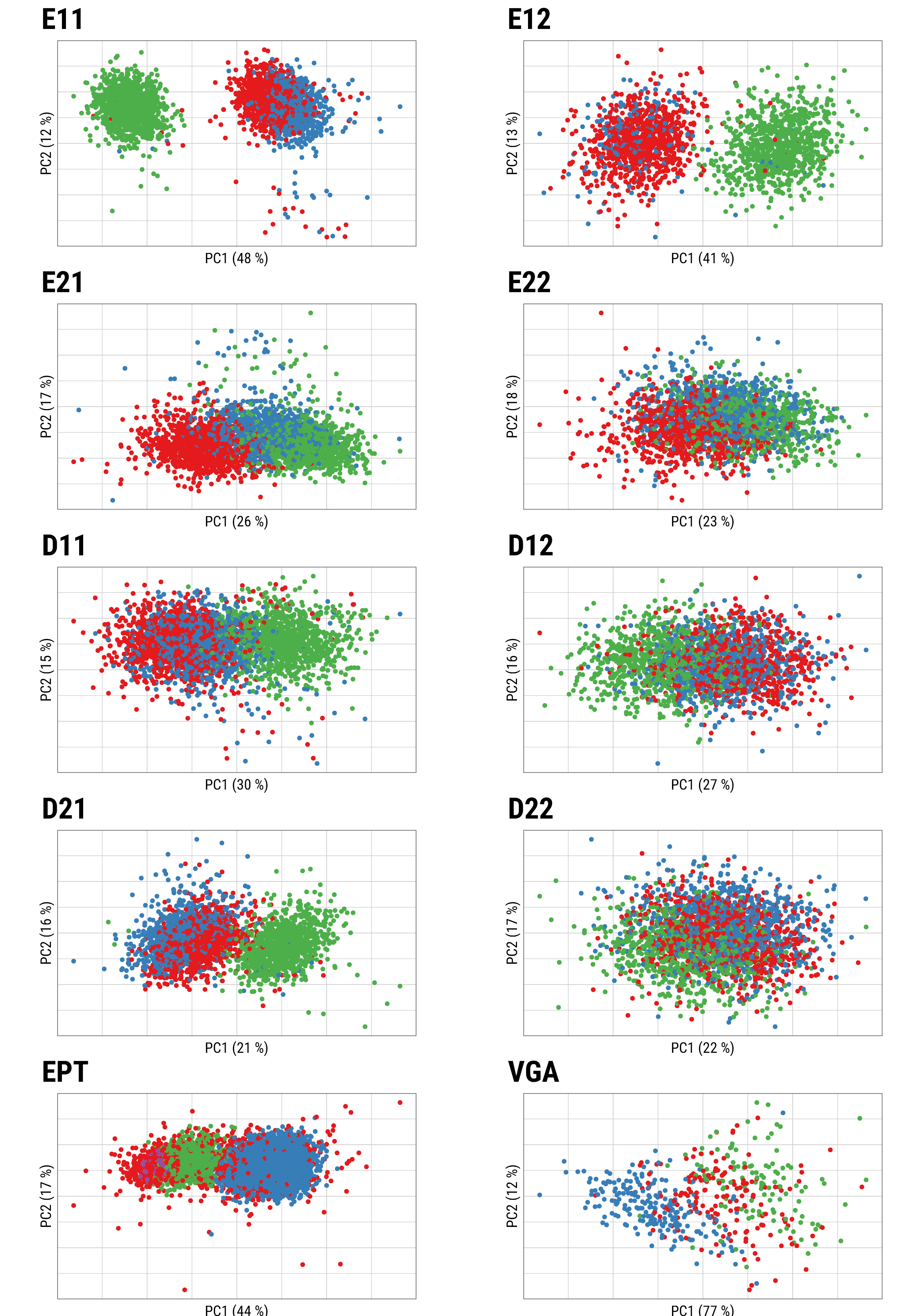
Figure 3: First two principal components projections of the spikes in the datasets coloured by class. Components’ explained variance is shown in the corresponding axis.

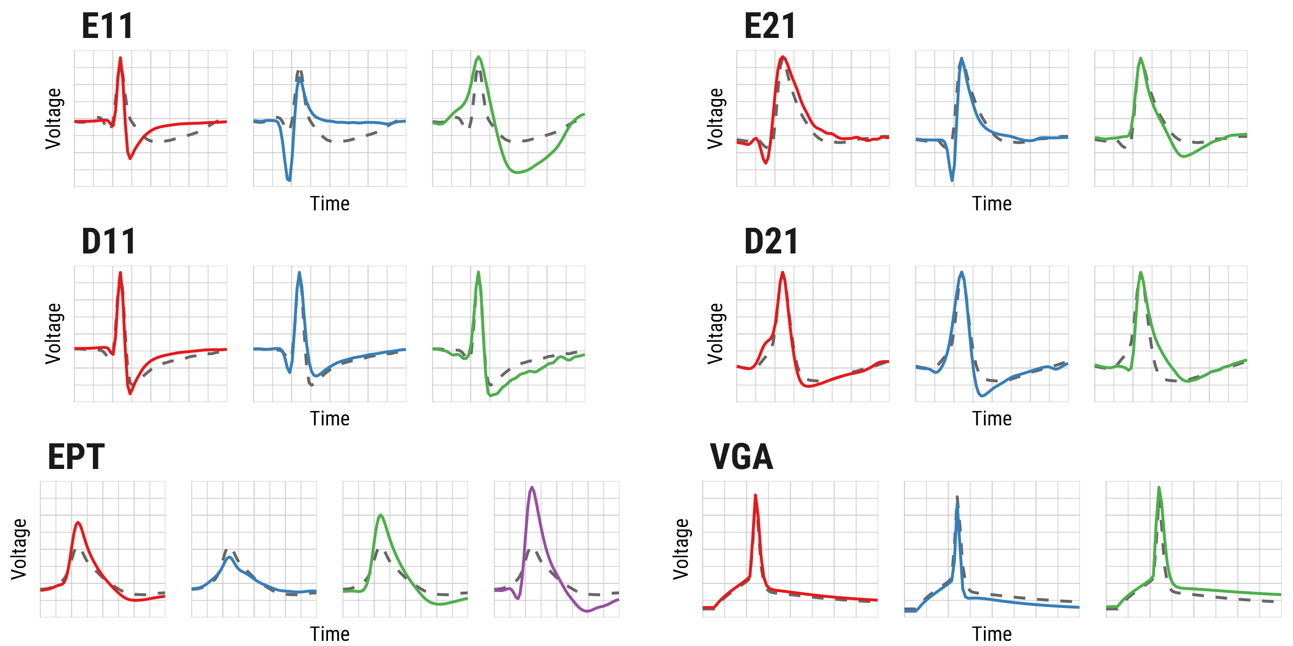
Figure 4: Spike means by class (solid lines) and global spike means (dashed) of datasets.

More specifically, the eight first datasets are simulated extracellular recordings first presented in [30]. The spikes fired by three different neurons are superimposed on background noise generated by small-amplitude spikes, mimicking the firing of distant neurons. In each dataset pair (E11 and E12, E21 and E22, etc.), the same three neurons are fired with mid and high background noise levels. The lower signal-to-noise ratio generates confusion between classes, as can be seen in Figure 3. Furthermore, these datasets are ordered in terms of increasing difficulty of correct clustering due to the similarity of the waveforms, as seen in Figure 4. The data have been preprocessed as in the cited works: spikes are detected with a threshold, $k=\mathrm{Med}(|\boldsymbol{z}|/0.6745)$ where $\boldsymbol{z}$ is the filtered signal, and the whole voltage traces have been fragmented into signals of 64 samples, each containing a single spike with its maximum aligned with the point 20. The noise artifacts erroneously detected as spikes, less than $4\%$ of the signals, have initially been discarded for the rest of the study.

Finally, the datasets EPT and VGA correspond to real recordings. EPT is a collection of extracellular spikes from four neurons of the temporal lobe of an epileptic patient, openly available in [29]. In this case, no preprocessing has been done, as the spikes are already cut into signals, with 64 samples and maxima aligned with point 20. In addition, the VGA has been created with data from [2], a repository of intracellular electrophysiological neuronal recordings. We selected signals from three GABAergic neuron types (Pvalb, Htr3a and Vip positive) of the mouse visual cortex; in particular, those generated by the short square stimulus with the lowest stimulus amplitude that elicited a single spike for each cell in the database. To facilitate the comparison, the signals have been down-sampled to have 64 samples, as in other datasets, aligning with the maximum at data point 20. Even though the mean spike waveforms are highly similar, as can be seen in Figure 4, the distinction of GABAergic neuron spikes is crucial as they radically differ in terms of physiological function [18].

4 Numerical Studies

In this Section, the MixFMM approach and the PCA (4 components) plus either KM (method PCA+KM) or GM (method PCA+GM), have been used to find clusters in the ten datasets described above. Specifically, the MixFMM₁ and MixFMM₃ homoscedastic models have been considered. A preliminary analysis with heteroscedastic models resulted in quite similar variance estimators across the datasets, as well as less accurate and more unstable solutions than those of the homoscedastic models. PCA+KM and PCA+GM have been considered as they are the most widely used clustering algorithms in SS, with better results in practice than wavelets, among other approaches, see [30, 14, 45]. The number of principal components in PCA ranges from two to four in the different SS applications. Here, only the results using four components are shown, as this choice gives better results in nine out of the ten datasets. For each of the clustering procedures and datasets, the best model from multiple initializations has been selected. Only ten initial values are needed for the MixFMM and PCA+KM approaches to obtain stable solutions; while the PCA+GM needed fifty initializations. Furthermore, the optimal number of clusters has been estimated with the most widely used method for each clustering procedure. A slope BIC heuristic for PCA+KM, and a combined integrated complete-data likelihood criterion plus BIC for PCA+GM, as proposed in [27, 41], respectively. The log-likelihood based approach, described in Section 2, has been used for the MixFMM_m models. Figure 5 shows the log-likelihoods for different numbers of clusters and the selection for each dataset.

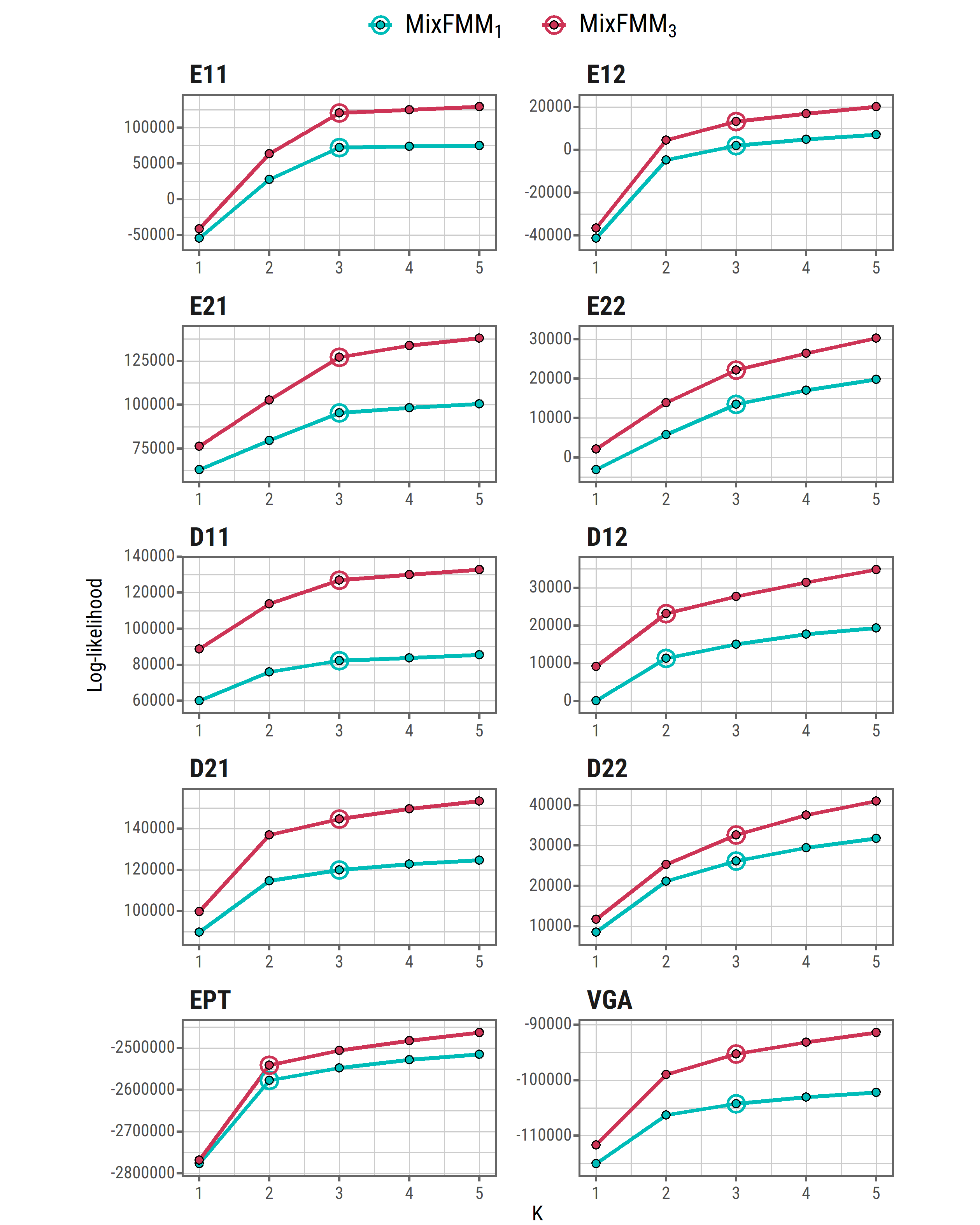
Figure 5: Log-likelihood of the MixFMM₁ and MixFMM₃ models for $K=\{2,3,4,5\}$ in each of the datasets. The selected number of clusters is highlighted with a circle.

Table 2: Estimated number of clusters, and index results for each dataset and method.

Number of clusters E11 E12 E21 E22 D11 D12 D21 D22 EPT VGA PCA+KM 3 2 3 3 3 3 3 3 3 3 PCA+GM 4 4 4 4 4 2 3 3 4 3 MixFMM₁ 3 3 3 3 3 2 3 3 2 3 MixFMM₃ 3 3 3 3 3 2 3 3 2 3 Accuracy E11 E12 E21 E22 D11 D12 D21 D22 EPT VGA PCA+KM 0.992 0.888 0.875 0.563 0.665 0.524 0.720 0.540 0.589 0.617 PCA+GM 0.960 0.958 0.851 0.347 0.905 0.510 0.640 0.613 0.680 0.710 MixFMM₁ 0.992 0.966 0.936 0.700 0.895 0.530 0.705 0.575 0.874 0.755 MixFMM₃ 0.994 0.976 0.966 0.761 0.941 0.541 0.743 0.606 0.874 0.746 Ball-Hall Index E11 E12 E21 E22 D11 D12 D21 D22 EPT VGA PCA+KM 1.153 3.344 1.162 2.852 1.182 2.492 0.967 2.471 18901 1400 PCA+GM 3.276 3.000 1.984 3.855 1.841 2.681 2.156 2.783 52804 1541 MixFMM₁ 1.154 2.971 1.102 2.807 1.088 2.697 0.967 2.542 21850 1230 MixFMM₃ 1.150 2.887 1.085 2.770 1.074 2.688 0.944 2.460 21734 1228 Davis-Bouldin Index E11 E12 E21 E22 D11 D12 D21 D22 EPT VGA PCA+KM 0.727 0.936 1.455 2.159 2.531 2.316 2.144 2.103 1.601 1.213 PCA+GM 2.411 1.140 2.421 1.735 3.149 2.118 3.291 2.883 2.355 1.580 MixFMM₁ 0.728 1.217 1.357 2.070 1.785 2.040 2.091 2.241 0.744 1.144 MixFMM₃ 0.726 1.159 1.341 1.993 1.717 2.024 2.070 2.112 0.742 1.144 Average Silhouette Width E11 E12 E21 E22 D11 D12 D21 D22 EPT VGA PCA+KM 0.552 0.439 0.250 0.117 0.126 0.120 0.173 0.128 0.262 0.280 PCA+GM 0.348 0.356 0.160 0.172 0.108 0.151 0.147 0.098 0.112 0.253 MixFMM₁ 0.551 0.348 0.282 0.124 0.193 0.162 0.173 0.121 0.512 0.326 MixFMM₃ 0.552 0.365 0.293 0.134 0.205 0.164 0.187 0.133 0.514 0.325

Table 2 summarizes the main results across different approaches, specifically the optimal number of clusters and the values of the validation indexes. The optimal number of clusters with the MixFMM corresponds to the real clusters in eight out of ten cases, which is comparable to or better than those of the other approaches. Note that the incorrect cases are characterized by a high level of noise. In terms of accuracy, which is likely the most relevant index, the MixFMM approach attains the best results in nine out of the ten datasets, achieving significant improvements over the PCA-based methods in some cases. The exception is dataset D22, in which PCA+GM is marginally better. Interestingly, PCA+KM achieves better results than PCA+GM, except in datasets where the average curves of the different classes are quite similar. Furthermore, the internal indexes confirm the better performance of the MixFMM approach against the PCA-based methods traditionally used in SS. More specifically, the low values of $\mathcal{BH}$ and $\mathcal{DB}$ for the MixFMM approaches indicate, on the one hand, that the clusters have a high cohesion, low dispersion and well-separated barycenters. On the other hand, the MixFMM clusters are composed of similar spikes distinguishable from others in near clusters by the high values of the $\mathcal{ASW}$.

While most of the results highlight the MixFMM₃ as the best all-around model, the MixFMM₁ should be considered a suitable alternative in specific cases, particularly in data with a high noise level, as the outstanding results in the real datasets demonstrate.

Comparing the results in Table 2 with results given in [45] in the common datasets, GM attains significantly better results in this work, probably due to R’s mclust being more optimized, flexible, and updated (mclust last version: December 2021; Matlab’s gmdistribution last version: before 2018).

Finally, in order to validate the robustness of the different approaches, the distribution of the accuracy has been studied across a hundred repetitions for the methods with ten initializations in each dataset. Figure 6 shows the associated boxplots, which illustrate that the MixFMM approach achieve an accurate solution independently of the initialization in all the scenarios analyzed, while the PCA-based methods fail, especially when spike waveform differences arise mostly from shape and not amplitude.

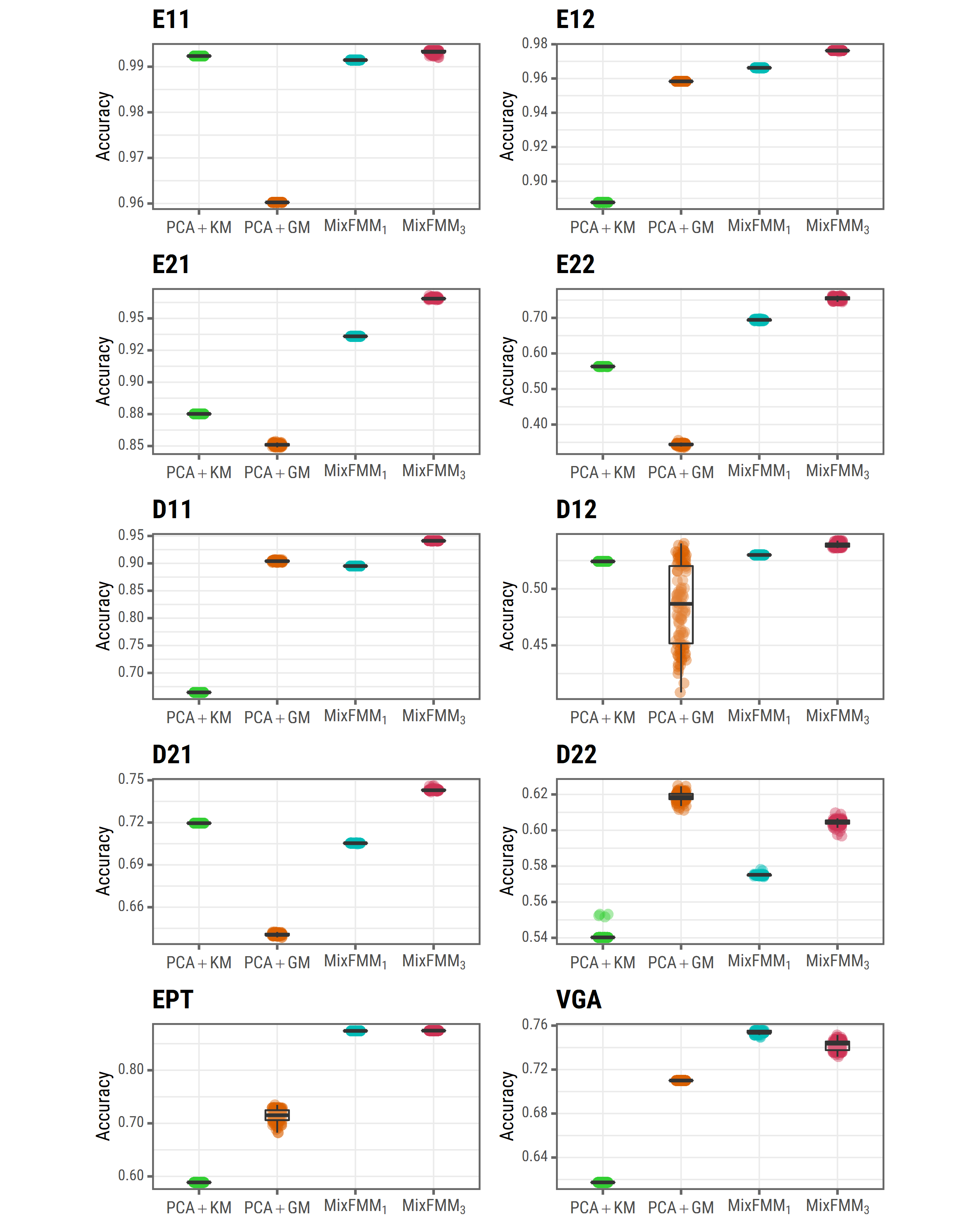
Figure 6: Boxplots of the accuracy across a hundred repetitions for each dataset and method.

5 Discussion

We present here a novel model-based functional data clustering method and prove its potential to solve the SS problem. In particular, we show that the MixFMM approach achieves better results than PCA-based methodologies often used in SS applications, achieving significant improvements in some scenarios, including very noisy cases. The MixFMM approach is based on using combinations of FMM waves to describe the signals, which allow a wide variety of waveforms to be described in a very simple and interpretable way. In particular, different FMM parameters account for variations in phase, amplitude, and shape.

The results of the MixFMM clustering entails interesting contributions in neuroscience. In particular, neuronal signals from the temporal lobe, such as EPT, are related to specific visual stimuli [33]. The function in the nervous system of the different kinds of GABAergic neurons is radically different, so the distinction of their signals is crucial. In VGA, signals from three types of neurons are differentiated: Pvalb-positive neurons, key in learning and memory processes, as detailed in [13]; Vip-positive neurons, related to circadian rhythms [24]; and Htr3a-positive neurons, related to bladder dysfunction [34]. In addition, the methodology can be adapted to cluster multichannel spike recordings [49], combining the information of FMM models for each channel, or with multivariate FMM models similar to those introduced in [39] to analyze ECG multilead signals.

Beyond its contribution to neuroscience, the MixFMM is presented as a general approach in functional clustering when oscillatory or quasi-oscillatory signals are the target. In a field in which the literature is ever-growing, and many excessively specific and complex proposals are arising, the need for flexible and robust proposals is vital. The MixFMM assembles all of these characteristics with a simple but rich parametric formulation that allows differences in phase and/or amplitude to be taken into account. Oscillatory signals appear in astronomy, economy, spectrometry, environmental science, medical imaging, or electrocardiography, among other fields. In addition, from a theoretical perspective, many extensions of the basic mixture framework could be explored, such as a regularized estimation algorithm or the inclusion of mixed-effects [9].

Finally, one limitation of the proposed methodology is its computational time. It could be significantly reduced by implementing the parameter search in a more computationally efficient programming language, such as C, and using GPU-based computing.

References

- [1] Serhat Akhanli and Christian Hennig. Comparing clusterings and numbers of clusters by aggregation of calibrated clustering validity indexes. Statistics and Computing, 30:1523–1544, 2020.
- [2] Allen Institute for Brain Science. Allen cell types database, 2021. Available in https://celltypes.brain-map.org/data.
- [3] Allen Institute for Brain Science. Allen SDK. Allen Institute, 2021. Python package version v2.13.0.
- [4] Lucien Birgé and Pascal Massart. Minimal penalties for gaussian model selection. Probability Theory and Related Fields, 138:33–73, 2007.
- [5] Charles Bouveyron, Etienne Côme, and Julien Jacques. The discriminative functional mixture model for a comparative analysis of bike sharing systems. The Annals of Applied Statistics, 9(4):1726–1760, 2015.
- [6] Gyorgy Buzsáki. Large-scale recording of neuronal ensembles. Nature Neuroscience, 7:446–51, 2004.
- [7] David Carlson and Lawrence Carin. Continuing progress of spike sorting in the era of big data. Current Opinion in Neurobiology, 55:90–96, 2019.
- [8] Carmen Rocío Caro-Martín, José M. Delgado-García, Agnès Gruart, and Raudel Sánchez-Campusano. Spike sorting based on shape, phase, and distribution features, and k-tops clustering with validity and error indices. Scientific reports, 8(1):1–28, 2018.
- [9] Faicel Chamroukhi and Hien D. Nguyen. Model-based clustering and classification of functional data. WIREs Data Mining and Knowledge Discovery, 9(4):e1298, 2019.
- [10] Gerda Claeskens, Emilie Devijver, and Irène Gijbels. Nonlinear mixed effects modeling and warping for functional data using B-splines. Electronic Journal of Statistics, 15(2):5245 – 5282, 2021.
- [11] Arthur Pentland Dempster, Nan Laird, and Donald Rubin. Maximum likelihood from incomplete data via the em algorithm. Journal of the Royal Statistical Society: Series B (Methodological), 39(1):1–22, 1977.
- [12] Bernard Desgraupes. clusterCrit: Clustering Indices. University of Paris Ouest, 2018. R package version 1.2.8.
- [13] Flavio Donato, Santiago Rompani, and Pico Caroni. Parvalbumin-expressing basket-cell network plasticity induced by experience regulates adult learning. Nature, 504:272–276, 2013.
- [14] Chaitanya Ekanadham, Daniel Tranchina, and Eero P. Simoncelli. A unified framework and method for automatic neural spike identification. Journal of Neuroscience Methods, 222:47–55, 2014.
- [15] Itziar Fernández, Alejandro Rodríguez-Collado, Yolanda Larriba, Adrian Lamela, et al. FMM: An R package for modeling rhythmic patterns in oscillatory systems. The R Journal, 2022. In press. Preprint available in https://arxiv.org/abs/2105.10168.
- [16] María Luz López García, Ricardo García-Ródenas, and Antonia González Gómez. K-means algorithms for functional data. Neurocomputing, 151:231–245, 2015.
- [17] Madison Giacofci, Sophie Lambert-Lacroix, Guillemette Marot, and Franck Picard. Wavelet-based clustering for mixed-effects functional models in high dimension. Biometrics, 69(1):31–40, 2013.
- [18] Nathan W. Gouwens, Staci A. Sorensen, Fahimeh Baftizadeh, Agata Budzillo, et al. Integrated morphoelectric and transcriptomic classification of cortical gabaergic cells. Cell, 183(4):935–953, 2020.
- [19] Plotly Technologies Inc. Collaborative data science. Plotly Technologies Inc., Montreal, QC, 2015.
- [20] Julien Jacques and Cristian Preda. Functional data clustering: a survey. Advances in Data Analysis and Classification, 8(3):24, 2014.
- [21] Wonyul Lee, Michelle F. Miranda, Philip Rausch, Veerabhadran Baladandayuthapani, et al. Bayesian semiparametric functional mixed models for serially correlated functional data, with application to glaucoma data. Journal of the American Statistical Association, 114(526):495–513, 2019.
- [22] Yaeji Lim, Hee-Seok Oh, and Ying Kuen Cheung. Multiscale Clustering for Functional Data. Journal of Classification, 36(2):368–391, 2019.
- [23] J. S. Marron, James Ramsay, Laura M. Sangalli, and Anuj Srivastava. Functional Data Analysis of Amplitude and Phase Variation. Statistical Science, 30(4):468–484, 2015.
- [24] Cristina Mazuski, Samantha Chen, and Erik Herzog. Different roles for vip neurons in the neonatal and adult suprachiasmatic nucleus. Journal of Biological Rhythms, 35(5):465–475, 2020.
- [25] Masoud Moghaddasi, Mahdi Aliyari Shoorehdeli, Zahra Fatahi, and Abbas Haghparast. Unsupervised automatic online spike sorting using reward-based online clustering. Biomedical Signal Processing and Control, 56:101701, 2020.
- [26] Juhyun Park and Jeongyoun Ahn. Clustering multivariate functional data with phase variation. Biometrics, 73(1):324–333, 2017.
- [27] Dau Pelleg and Andrew Moore. X-means: Extending k-means with efficient estimation of the number of clusters. In Proceedings of the 17th International Conf. on Machine Learning, pages 727–734, 2000.
- [28] Rodrigo Quian Quiroga. Simulated datasets, 2009. Available in https://leicester.figshare.com/articles/dataset/Simulated_dataset/11897595.
- [29] Rodrigo Quian Quiroga. Dataset: Human single-cell recording, 2019. Available in https://leicester.figshare.com/articles/Dataset_Human_single-cell_recording/11302427/1.
- [30] Rodrigo Quian Quiroga, Zoltan Nadasdy, and Yoram Ben-Shaul. Unsupervised Spike Detection and Sorting with Wavelets and Superparamagnetic Clustering. Neural Computation, 16(8):1661–1687, 2004.
- [31] R Core Team. R: A Language and Environment for Statistical Computing. R Foundation for Statistical Computing, Vienna, Austria, 2020.
- [32] Melinda Rácz, Csaba Liber, Erik Németh, Richárd Fiáth, et al. Spike detection and sorting with deep learning. Journal of Neural Engineering, 17:016038, 2019.
- [33] Hernan Gonzalo Rey, Carlos Pedreira, and Rodrigo Quian Quiroga. Past, present and future of spike sorting techniques. Brain research bulletin, 119:106–117, 2015.
- [34] Elaine Ritter and Michelle Southard-Smith. Dynamic expression of serotonin receptor 5-ht3a in developing sensory innervation of the lower urinary tract. Frontiers in Neuroscience, 10:592, 2017.
- [35] Alejandro Rodríguez-Collado and Cristina Rueda. Electrophysiological and transcriptomic features reveal a circular taxonomy of cortical neurons. Frontiers in Human Neuroscience, 15:684950, 2021.
- [36] Alejandro Rodríguez-Collado and Cristina Rueda. A simple parametric representation of the Hodgkin-Huxley model. PLOS ONE, 16(7):1–19, 2021.
- [37] Cristina Rueda, Yolanda Larriba, and Adrian Lamela. The hidden waves in the ecg uncovered revealing a sound automated interpretation method. Scientific Reports, 11:3724, 2021.
- [38] Cristina Rueda, Yolanda Larriba, and Shyamal D. Peddada. Frequency modulated Möbius model accurately predicts rhythmic signals in biological and physical sciences. Scientific Reports., 9(1):1–10, 2019.
- [39] Cristina Rueda, Alejandro Rodríguez-Collado, Itziar Fernández, Christian Canedo, et al. A unique cardiac electrophysiologic model, 2022. Preprint. Available in https://arxiv.org/abs/2202.03938.
- [40] Cristina Rueda, Alejandro Rodríguez-Collado, and Yolanda Larriba. A novel wave decomposition for oscillatory signals. IEEE Transactions on Signal Processing, 69:960–972, 2021.
- [41] Luca Scrucca, Michael Fop, T. Brendan Murphy, and Adrian E. Raftery. mclust 5: clustering, classification and density estimation using Gaussian finite mixture models. The R Journal, 8(1):289–317, 2016.
- [42] Niraj K. Sharma, Carlos Pedreira, Maria Centeno, Umair J. Chaudhary, et al. A novel scheme for the validation of an automated classification method for epileptic spikes by comparison with multiple observers. Clinical Neurophysiology, 128(7):1246–254, 2017.
- [43] Bryan Souza, Vítor Lopes dos Santos, João Bacelo, and Adriano Tort. Spike sorting with gaussian mixture models. Scientific Reports, 9:3627, 2019.
- [44] Jeyathevy Sukiban, Nicole Voges, Till A. Dembek, Robin Pauli, et al. Evaluation of spike sorting algorithms: Application to human subthalamic nucleus recordings and simulations. Neuroscience, 414:168–185, 2019.
- [45] Rakesh Veerabhadrappa, Masood Ul Hassan, James Zhang, and Asim Bhatti. Compatibility evaluation of clustering algorithms for contemporary extracellular neural spike sorting. Frontiers in Systems Neuroscience, 14:34, 2020.
- [46] Lucas Vendramin, Ricardo J. G. B. Campello, and Eduardo R. Hruschka. Relative clustering validity criteria: A comparative overview. Statistical Analysis and Data Mining: The ASA Data Science Journal, 3(4):209–235, 2010.
- [47] Pan Ke Wang, Sio Hang Pun, Chang Hao Chen, Elizabeth A. McCullagh, et al. Low-latency single channel real-time neural spike sorting system based on template matching. PLOS ONE, 14(11):1–30, 2019.
- [48] Hadley Wickham. ggplot2: Elegant Graphics for Data Analysis. Springer - Verlag New York, second edition, 2016.
- [49] Pierre Yger, Giulia LB Spampinato, Elric Esposito, Baptiste Lefebvre, et al. A spike sorting toolbox for up to thousands of electrodes validated with ground truth recordings in vitro and in vivo. eLife, 7:e34518, 2018.
- [50] Qingzhi Zhong, Huazhen Lin, and Yi Li. Cluster non-gaussian functional data. Biometrics, 77(3):852–865, 2020.