Inference in Linear Dyadic Data Models
with Network Spillovers

When using dyadic data (i.e., data indexed by pairs of units), researchers typically assume a linear model, estimate it using Ordinary Least Squares and conduct inference using “dyadic-robust” variance estimators. The latter assumes that dyads are uncorrelated if they do not share a common unit (e.g., if the same individual is not present in both pairs of data). We show that this assumption does not hold in many empirical applications because indirect links may exist due to network connections, generating correlated outcomes. Hence, “dyadic-robust” estimators can be biased in such situations. We develop a consistent variance estimator for such contexts by leveraging results in network statistics. Our estimator has good finite sample properties in simulations, while allowing for decay in spillover effects. We illustrate our message with an application to politicians’ voting behavior when they are seating neighbors in the European Parliament.

Keywords: Dyadic data, Networks, Inference, Cross-sectional dependence, Congressional Voting.

1 Introduction

Dyadic data is categorized by the dependence between two sets of sampled units (dyads). For example, exports between the U.S. and Canada depend on both countries (and, plausibly, their characteristics). This contrasts to classical data in the social sciences that only depends on a single unit of observation (e.g., the GDP of the U.S., or a politician’s vote in a roll-call).

The empirical relevance of dyadic data is showcased by its widespread use, which has increased over the past two decades (Graham (2020a) provides an extensive review). For example, applications are found in political economy (correlation in voting behavior in Parliament across seating neighbors, Harmon et al. (2019)), international political economy and trade (export-import outcomes across countries, Anderson and van Wincoop (2003)), international relations (Hoff and Ward (2004), for a salient example), among many others. In fact, dyadic data is considered to be dominant in quantitative international relations (Poast, 2016). In these examples, applied researchers typically model the dependence between dyadic outcomes and observable characteristics using a linear model, which they then estimate using Ordinary Least Squares (OLS). However, inference on such estimators for the linear parameters is more complex.

The main approach in recent applied work has been the use of the so-called “dyadic-robust” estimators (e.g., Cameron et al. (2011), Aronow et al. (2015), and Tabord-Meehan (2019), among others). Such estimators build on the widely-used assumption in dyadic data that the error terms for dyad $(i,j)$ and for dyad $(k,l)$ can only be correlated if they share a unit (see Aronow et al. (2015) and Tabord-Meehan (2019) for a discussion; Cameron and Miller (2014) for a review).

In this paper, we first argue that such an assumption does not hold in many applications using dyadic data where dyads may be indirectly connected along a network. Figure 1 presents a simple example in the context of politicians in Congress, whose votes or decisions depend on their seating neighbors. It is completely possible that behavior across dyads $(A,B)$ and $(C,D)$ might be correlated along unobservables because they have many indirect connections (in the figure, through $A$ sitting next to $B$, who sits next to $C$). We show that such spillovers invalidate the assumptions for consistency of existing “dyadic-robust” variance estimators through generating interdependence, implying that they are biased for the true asymptotic variance when dyads may be correlated even when they do not share a common unit.

Figure 1: Hypothetical Example of a Network in Parliament

• Notes: The left figure shows a hypothetical example of politician networks based on seating arrangements: $A$ sits beside $B$, who sits beside $C$, who sits beside $D$. The right-hand figure illustrates the resulting network among active dyads. As dyads $(A,B)$ and $(B,C)$ share a unit, they are indirectly linked in the dyadic network. However, though dyads $(A,B)$ and $(C,D)$ do not have a politician in common, they might still be correlated through two indirect links: namely, $B$ sits beside $C$, who sits beside $D$. Hence, $D$’s actions can affect politician $A$.

To deal with these issues, we develop a consistent variance estimator that explicitly accounts for such network spillovers even with dyadic data, thereby complementing existing approaches (e.g., Aronow et al. (2015)). We prove that our proposed variance estimator is consistent for the true variance of the OLS estimator in linear models with dyadic data when the cross-sectional dependence follows an observed (exogenous) network. Our main insight is that the dependence across all dyads, including indirect spillovers, can be rewritten as correlations across a specific network over dyads. This allows us to apply the framework of Kojevnikov et al. (2021) to such network random variables, although here it is a network over dyads, rather than individuals. Monte Carlo simulations show that our proposed estimator has good finite sample properties and outperforms other estimators for the relevant contexts.

To help practitioners, we then provide a step-by-step guideline on whether our estimator may be appropriate to their context. As we describe, this choice depends on: (i) whether spillovers from indirectly connected dyads are likely to be present, (ii) whether the researcher observes/constructs the network among dyads through which spillovers propagate, and (iii) whether those spillovers are likely to be persistent. Our variance estimator is consistent for the asymptotic variance of the OLS estimator even under (i)-(iii). And our estimator can account for decay in propagation, as Corollary 3.1 and Example 3.1 illustrate. On the other hand, if decay is very high, or spillovers along the network do not exist, then those same results imply that the estimator of Aronow et al. (2015) will also be consistent.

Finally, we illustrate the extent to which neglecting network spillovers with dyadic data may bias inference results. Beyond Monte Carlo simulations, we revisit the application in Harmon et al. (2019) of voting in the European Parliament. The authors study whether random seating arrangements (based on naming conventions) induce neighboring politicians to agree with one another in policy votes. The outcome, whether politicians $i$ and $j$ vote the same way on a policy, is dyadic in nature. However, $i$ and $j$’s votes may be positively correlated even if they are not neighbors: for instance, $i$ and $j$ may sit on either side of common neighbors $k$ and $l$, who influence them both, and this seating arrangement is observed. This chain of influences is sufficient to induce strong positive correlation across non-dyads. We show that neglecting such higher order spillovers has significant empirical consequences: their estimated variance using the estimator in Aronow et al. (2015) is roughly $22\%$ smaller than using our consistent estimator accounting for such spillovers; while the estimate based on the Eicker-Huber-White estimator ignoring spillovers is approximately 73% smaller than our proposal, consistent with the arguments of Erikson et al. (2014).

1.1 Related Literature

The use of dyadic data in Political Science has a rich history, particularly in International Relations. However, empirical challenges with such models are well known – see Poast (2016) for a historical overview. Early on, the concerns were mostly about model specification, including the error term. This includes the 2001 special issue of International Organization, mostly focusing on the use of fixed effects. More recently, Erikson et al. (2014) pointed out that ignoring dependence across dyads can lead to erroneous hypothesis testing, as computed standard errors would be too small. Hoff and Ward (2004) and Minhas et al. (2019); Minhas et al. (2022) suggest including random coefficients and latent variables to account for dependencies across dyads. Our approach explicitly accounts for the whole network of interdependencies across dyads, which can go beyond third-order dependences (assumed in Minhas et al. (2019); Minhas et al. (2022)). It does so by using asymptotic inference, rather than Bayesian (Minhas et al., 2019; Minhas et al., 2022) or randomized inference (Erikson et al., 2014).

As a result, our paper is directly related to the literature on (asymptotic) inference in regression analysis with dyadic random variables. Aronow et al. (2015) and Tabord-Meehan (2019) consider OLS estimation and inference in a linear dyadic regression model. Meanwhile, Graham (2020a) and Graham (2020b) explore a likelihood-based approach to dyadic regression models, while Graham et al. (2022) and Chiang and Tan (2022) provide results for kernel density estimation in dyadic regression models. While useful to allow for correlations along time and within such groups, this separable structure may be inappropriate for environments where spillovers follow a complex form of dependence along a network. As alluded to previously, all such papers assume that dyads are uncorrelated unless they share a common unit, thereby ignoring dependence across indirectly linked dyads, while our estimator explicitly captures the higher order correlation across dyads along the dyadic network.

However, we emphasize that neither approach subsumes the other. The papers cited above leave the dependence within “clusters” (groups of dyads that share units) unrestricted, but assume independence across such clusters. This is akin to the literature with one-way clustering (e.g., Hansen and Lee (2019)). By comparison, our approach restricts such dependence among groups of dyads that share units (i.e., dependence is assumed to follow the observed network), but allows for dependence across such “clusters” of dyads along the dyadic network. Which approach to pursue using dyadic data depends on the researchers’ applications and how they fit such assumptions.

2 Set-up

Assume that we observe a cross section of $N\in\mathbbm{N}$ individuals located along a network – the latter interpretable as politicians, countries, firms, or other observation units depending on the context. The dyads present in the $N$-individual network (i.e., among the $\tbinom{N}{N-1}$ possible dyads), are called active dyads, so that the dyad for two units $i$ and $j$ (e.g., politicians, countries) is denoted as some $m$. The set of active dyads is denoted $\mathcal{M}_{N}$ and $M$ denotes the cardinality of that set.

We assume that each dyad $m$ is endowed with a triplet of dyad-specific variables, forming a triangular array $\{(y_{M,m},x_{M,m},\varepsilon_{M,m})\}_{m\in\mathcal{M}_{N}}$ with respect to $M$, where $y_{M,m}\in\mathbbm{R}$ is a one-dimensional observable outcome, $x_{M,m}\in\mathbbm{R}^{K}$ is a $K$-dimensional vector of observable characteristics with $K\in\mathbbm{N}$, and $\varepsilon_{M,m}\in\mathbbm{R}$ is a one-dimensional random error term that is not observable to the researcher. We only consider exogenous network formation and the network is assumed to be observable. These conditions are summarized in the following assumption:

Assumption 2.1 (Exogenous and Observable Dyadic Networks).

The network among dyads is assumed to be conditionally independent of $\{\varepsilon_{M,m}\}_{m\in\mathcal{M}_{N}}$. Furthermore, this network among the $N$ individuals is assumed to be observable.

While such assumptions are standard in models of dyadic networks, they seem particularly appropriate when units or dyad pairs are linked across geographical, physical, or ex-ante social relations (e.g., family ties). This includes capturing neighboring and regional spillovers across countries, as often done in international relations, or exogenous seating arrangements in Parliament, as illustrated in the examples in the next section.

The subsequent arguments require us to distinguish between a pair of dyads who share a member (i.e., who are directly linked – which we call, adjacent) and a pair of dyads who are directly or indirectly linked (which we call, simply, connected).

Definition 2.1 (Adjacent & Connected Dyads).

Two active dyads $m$ and $m^{\prime}$ are said to be adjacent if they have an individual in common; and they are called connected if they are linked through pairs of adjacent dyads.

In Figure 1, dyad (A,B) is adjacent to (B,C), and connected with, though not adjacent to, (C,D). Hence, the adjacency relationship constitutes a network structure among active dyads, and thus, a network over individuals can be transformed to one over active dyads. For example, the right-hand side panel of Figure 1 provides a network over pairs of voting politicians (i.e., active dyads). We define the geodesic distance between two connected dyads $m$ and $m^{\prime}$ to be the smallest number of adjacent dyads between them. Note that adjacent dyads are a special case of connected dyads with geodesic distance equal to one.

2.1 The Linear Model

2.1.1 Set-up & Identification

The cross-sectional model of interest takes the form of the linear network-regression model: for any $N\in\mathbbm{N}$,

$$y_{M,m}=x_{M,m}^{\prime}\beta+\varepsilon_{M,m}\ \ \ \ \ \forall m\in\mathcal{M}_{N},$$ (1)

where

$$Cov(\varepsilon_{M,m},\varepsilon_{M,m^{\prime}}\mid X_{M})=0\quad\text{unless $m$ and $m^{\prime}$ are connected},$$ (2)

and $\beta$ is a $K\times 1$ vector of the regression coefficients and $X_{M}$ denotes the $M\times K$ matrix that records the observed dyad-specific characteristics, i.e., $X_{M}\coloneqq[x_{M,1},\ldots,x_{M,M}]^{\prime}$.

In this paper, we assume that $\beta$ is identified, which follows from standard assumptions on strict exogeneity, lack of multicollinearity and the existence of finite second moments of $y_{M,m}$ and $x_{M,m}$. (For completeness, see Assumption B.1 and Proposition B.1 in Appendix).

We note that equation (2) allows for there to be spillovers across the error terms even when dyads $m$ and $m^{\prime}$ are not adjacent, as long as they are connected through indirect links. By comparison, applied researchers such as Harmon et al. (2019) and Lustig and Richmond (2020) (and the estimators of Aronow et al. (2015) and Tabord-Meehan (2019)) consider a variant of the linear regression (1) under the assumption

$$Cov(\varepsilon_{M,d(i,j)},\varepsilon_{M,d(k,l)}\mid x_{M,d(i,j)},x_{M,d(k,l)})=0\hskip 14.22636pt\text{unless \quad$\{i,j\}\cap\{k,l\}\neq\emptyset$},$$ (3)

with $m=d(i,j)$ representing the dyad between $i$ and $j$. This specific assumption would be equivalent to setting:

$$Cov(\varepsilon_{M,m},\varepsilon_{M,m^{\prime}}\mid X_{M})=0\hskip 14.22636pt\text{unless $m$ and $m^{\prime}$ are adjacent}.$$ (4)

2.1.2 Examples

Whether to allow indirect spillovers as in (2) or not (as in (4)) depends on the researchers’ applications. We now present two examples where our approach may be preferable.

Example 2.1 (Gravity Model of Bilateral Trade Flow).

A researcher is studying the trade flow from country $i$ to $j$, with (log) exports from $i$ to $j$ denoted $y_{ij}$. Following the literature, (s)he assumes $y_{ij}$ follows the structural gravity equation (e.g., Eaton and Kortum (2002); Anderson and van Wincoop (2003); Melitz (2003); Helpman et al. (2008)):

$$y_{ij}=\alpha+\beta z_{ij}+\gamma\sum_{k\neq i}g_{ki}y_{ki}+\eta_{ij},$$ (5)

where $z_{ij}$ represents a dyadic characteristic of $i$ and $j$, such as the shipping cost, whether both countries are democratic (e.g., Mansfield et al., 2000), or whether both participate in WTO/GATT (e.g., Gowa and Kim, 2005); $\sum_{k}g_{ki}y_{ki}$ is the amount $i$ spends on imports ($g_{ki}$ equals one if country $i$ purchases goods from country $k$ and zero otherwise), and $\eta_{ij}$ captures unobserved heterogeneity pertaining to the trade flow between countries $i$ and $j$.

To see our main point, suppose there are only four countries ($1$, $2$, $3$ and $4$) which trade, where country $1$ exports to country $2$, which in turn exports to country $3$, and country $3$ exports to country $4$. Equation (5) then simplifies to: $y_{12}=\alpha+\beta z_{12}+\eta_{12}$,
$y_{23}=\alpha+\beta z_{23}+\gamma y_{12}+\eta_{23}$, and henceforth. Rearranging these equations implies that the trade flow from country $3$ to $4$ can be written as:

$$y_{34} =\alpha+\alpha\gamma+\alpha\gamma^{2}+\gamma^{2}\beta z_{12}+\gamma\beta z_{23}+\beta z_{34}+\gamma^{2}\eta_{12}+\gamma\eta_{23}+\eta_{34}.$$

Therefore, $Cov(y_{12},y_{34}\mid z)=\gamma^{2}Var(\eta_{12}\mid z)\neq 0$, where $z\equiv\{z_{12},z_{23},z_{34}\}$. Hence, there can be non-zero correlation between trade flows $y_{12}$ and $y_{34}$ even if they do not have a country in common. This is because an idiosyncratic shock to an upstream country can propagate through the trade network.

Example 2.2 (Legislative Voting).

A researcher is interested in whether seating arrangements in legislatures can affect a politician’s behavior, $y_{i}$ (e.g., propensity to vote “Yes” on a roll-call, as Harmon et al. (2019), or the amount of co-sponsoring, as Saia (2018); Lowe and Jo (2021), among others). For concreteness, suppose there are four politicians with the seating arrangements given by Figure 1.

The researchers posit that $i$’s behavior can be influenced by the (average) of its seating neighbors’ own voting behavior through a parameter $\gamma$ as follows:

$$y_{A}=\alpha+\gamma y_{B}+\eta_{A},\quad y_{B}=\alpha+\gamma\frac{y_{A}+y_{C}}{2}+\eta_{B}$$ (6)

$$y_{C}=\alpha+\gamma\frac{y_{B}+y_{D}}{2}+\eta_{C},\quad y_{D}=\alpha+\gamma y_{C}+\eta_{D}$$ (7)

If $\gamma\neq 0$, $A$ is affected by their neighbor $B$, while $B$ is affected by both of its neighbors ($A$ and $C$) and so forth. The researcher is interested in whether neighbors’ decisions are more highly correlated than the decisions among non-neighbors.

Denote $y_{ij}$ as the dyadic outcome of interest (e.g., a measure of correlation between $i$ and $j$’s decisions). Both $y_{AB}$ and $y_{CD}$ involve $y_{B}$ and $y_{C}$, which are themselves a function of $\eta_{B}$ and $\eta_{C}$. Hence, $Cov(y_{AB},y_{CD})\neq 0$, even if the two pairs of legislators do not share a common member.

2.1.3 Estimation

Throughout this paper, we focus on the Ordinary Least Squares (OLS) estimator of $\beta$, denoted by $\hat{\beta}$. Under the assumptions above, we can write

$$\hat{\beta}-\beta =\Bigg{(}\sum_{j\in\mathcal{M}_{N}}x_{M,j}x_{M,j}^{\prime}\Bigg{)}^{-1}\sum_{m\in\mathcal{M}_{N}}x_{M,m}\varepsilon_{M,m}.$$ (8)

It is straightforward to verify that $\hat{\beta}$ is unbiased for $\beta$ under our identification conditions (Assumption B.1). However, a consistency result is by no means trivial due to the dependence along the network which induces a complex form of cross-sectional dependence, hindering a naïve application of the standard theory for independently and identically distributed ($i.i.d.$) random vectors. This is clarified in Section 3.1. Before that, we provide a heuristic overview of the main point of our paper in this setting.

2.2 Outline of Our Procedure

2.2.1 Inference

Inference about $\beta$ is based on a normal approximation of the distribution of $\hat{\beta}$ around $\beta$. We focus on hypothesis testing conducted using the expression:

$$\big{(}\widehat{Var}(\hat{\beta})\big{)}^{-\frac{1}{2}}(\hat{\beta}-\beta),$$ (9)

where $\widehat{Var}(\hat{\beta})$ is a consistent estimator of the asymptotic variance of $\hat{\beta}$. Our main result in Section 3.4 is providing such an appropriate estimator, which takes the form:

$$\widehat{Var}(\hat{\beta})\coloneqq\Bigg{(}\sum_{k\in\mathcal{M}_{N}}x_{k}x_{k}^{\prime}\Bigg{)}^{-1}\Bigg{(}\sum_{m\in\mathcal{M}_{N}}\sum_{m^{\prime}\in\mathcal{M}_{N}}\kappa_{m,m^{\prime}}h_{m,m^{\prime}}\hat{\varepsilon}_{m}\hat{\varepsilon}_{m^{\prime}}x_{m}x_{m^{\prime}}^{\prime}\Bigg{)}\Bigg{(}\sum_{k\in\mathcal{M}_{N}}x_{k}x_{k}^{\prime}\Bigg{)}^{-1},$$ (10)

where $\kappa_{m,m^{\prime}}$ is an appropriate kernel function that will formally be defined in Section 3.4; $h_{m,m^{\prime}}$ represents an indicator function that takes one if dyads $m$ and $m^{\prime}$ are connected and zero otherwise; and $\hat{\varepsilon}_{m}\coloneqq y_{m}-x_{m}^{\prime}\hat{\beta}$.

This paper derives conditions under which $\widehat{Var}(\hat{\beta})$ is consistent for the asymptotic variance of $\hat{\beta}$. Before doing so, let us compare the variance estimator (10) with an often used estimator based on one-way clustering of dyad groupings.

Remark 2.1 (Dyadic-Robust Variance Estimator).

An increasing number of applied researchers, such as Harmon et al. (2019) and Lustig and Richmond (2020), estimate model (1) and conduct inference, using the following dyadic-robust variance estimators proposed by Aronow et al. (2015) and Tabord-Meehan (2019):

$$\widehat{Var}(\hat{\beta})\coloneqq\Bigg{(}\sum_{k\in\mathcal{M}_{N}}x_{k}x_{k}^{\prime}\Bigg{)}^{-1}\Bigg{(}\sum_{m\in\mathcal{M}_{N}}\sum_{m^{\prime}\in\mathcal{M}_{N}}\mathbbm{1}_{m,m^{\prime}}\hat{\varepsilon}_{m}\hat{\varepsilon}_{m^{\prime}}x_{m}x_{m^{\prime}}^{\prime}\Bigg{)}\Bigg{(}\sum_{k\in\mathcal{M}_{N}}x_{k}x_{k}^{\prime}\Bigg{)}^{-1},$$ (11)

where $\mathbbm{1}_{m,m^{\prime}}$ equals one if dyads $m$ and $m^{\prime}$ are adjacent and zero otherwise.

Note that the use of the dyadic-robust variance estimator sets cases in which two dyads are not adjacent, but connected, to zero. Meanwhile, our estimator (10) accounts for network spillovers by accommodating the correlation across both adjacent and connected dyads. As our examples above suggest, the structure of the variance estimator (11) may not be compatible with indirect spillovers in some settings, which should assume the specification (2) instead. This suggests that the dyadic-robust variance estimator may be inconsistent when there is cross-sectional dependence along a network over dyads: i.e., when non-adjacent dyads can still affect the correlation structure and outcomes of dyad $m$. This conjecture is formally proven in Corollary 3.1 and illustrated in Monte Carlo simulations in Section 4. We note that this is a feature of applying such dyadic-robust variance estimators to network spillovers, and not a feature of those estimators per se.

In order to validate the test statistic (9) for inference, this paper establishes the consistency and asymptotic normality of $\hat{\beta}$ and develops a consistent network-robust estimator for the asymptotic variance when the correlation structure is given by (2).

2.2.2 A Step-by-Step Guide on Implementation

Researchers interested in the linear specification (1) may find the following guidelines useful when deciding whether to use our proposed estimator (10).

1. The researcher should first ask whether spillovers from indirectly connected dyads are likely to be present (and not decay immediately) in their set-up: i.e., is equation (2) a more appropriate assumption than equation (4)?

   While this depends on the specific application, Examples 2.1-2.2 illustrate models where that is likely to be the case. And condition (17) provides a notion of how much persistence is needed for a bias to appear. As we show below, these insights are robust to decaying spillover effects (see Corollary 3.1, Example 3.1, and the associated simulation results).

2. If such spillovers of unobservables are likely to exist, are they governed by an exogenous and observable network (Assumption 2.1), such as physical, geographical or social (e.g., family ties)? If so, the proposed estimator is appropriate under regularity conditions.

3. One can implement our estimator by: (i) choosing a kernel (e.g., rectangular, see Section 3.4), (ii) setting the lag-truncation, $b_{M}$ (either by a known value, or adaptively by $b_{M}=2\log(M)/\log(\max(average~{}degree,1.05))$, where $M$ is the number of dyads and we use the average degree of the dyadic network, (iii) plugging-in those choices into equation (10).

   This estimator is consistent under regularity conditions, even when spillovers decay, and shows good finite-sample properties in the simulations below.

3 Theoretical Results

3.1 Network Dependent Processes

Let $Y_{M,m}$ be a random vector defined as

$$Y_{M,m}\coloneqq x_{M,m}\varepsilon_{M,m},$$ (12)

and denote $\mathcal{C}_{M}\coloneqq\{x_{M,m}\}_{m\in\mathcal{M}_{N}}$. From equations (8) and (12) we can write

$$\hat{\beta}-\beta=\Bigg{(}\frac{1}{M}\sum_{j\in\mathcal{M}_{N}}x_{M,j}x_{M,j}^{\prime}\Bigg{)}^{-1}\frac{1}{M}\sum_{m\in\mathcal{M}_{N}}Y_{M,m}.$$ (13)

Our interest lies in proving the asymptotic properties of $\hat{\beta}$ taking advantage of the expression (13). However, the presence of $\varepsilon_{M,m}$ in $Y_{M,m}$, which is allowed to be correlated along the network over active dyads, renders our approach nonstandard. The canonical results about independently and identically distributed ($i.i.d.$) random variables are by no means applicable due to the complex form of dependence inherent to $\varepsilon_{M,m}$. Dyadic-robust estimators (e.g., Aronow et al. (2015) and Tabord-Meehan (2019)) only account for correlations between adjacent dyads. This may be appropriate in some settings, but not when there may be indirect spillovers, as in specification (1) – (2). Thence, the right hand side of (13) cannot simply be embedded in other widely-studied variants of dependent random vectors, including spatially-correlated and time-series data.

The main insight of this paper is that the spillovers across connected – even if not adjacent – dyads, can be rewritten as the dependence of $Y_{M,m}$’s along the network of active dyads (hereby, referred to as the “network”). This transformation allows us to embrace such complex cross-sectional dependence and appropriately rewrite the problem so that recent results on network dependent random variables (Kojevnikov et al., 2021) can be applied. Our results then allow for correlations of random variables given a common shock as explicitly dictated by distances between them on the dyadic network. Our notion of dependence restricts the covariance between the random variables for any two sets of dyads $A$ and $B$, $Y_{M,A}$ and $Y_{M,B}$, which are at a distance $s$ from one another, to be bounded and to decrease as $s$ goes to infinity. Indeed, this covariance is controlled by a sequence of (random) coefficients $\theta_{M,s}$, which capture the strength of covariation net of scaling, analogous to correlation coefficients. As the minimum distance, $s$, between $A$ and $B$ grows, the dependence $\{\theta_{M,s}\}$ between $Y_{M,A}$ and $Y_{M,B}$, tends to zero. A formal description is provided in Appendix A.

3.2 Definitions

As will become transparent shortly, asymptotic theories for $\hat{\beta}$ rest on tradeoffs between the correlation of the network-dependent random vectors (i.e., the dependence coefficients) and the denseness of the underlying network. To measure the denseness, we first define two concepts of neighborhoods: for each $m\in\mathcal{M}_{N}$ and $s\in\mathbbm{N}\cup\{0\}$,

$$\mathcal{M}_{N}(m;s)\coloneqq\{m^{\prime}\in\mathcal{M}_{N}:\rho_{M}(m,m^{\prime})\leq s\},$$

$$\mathcal{M}_{N}^{\partial}(m;s)\coloneqq\{m^{\prime}\in\mathcal{M}_{N}:\rho_{M}(m,m^{\prime})=s\},$$

where $\rho_{M}(m,m^{\prime})$ denotes the geodesic distance between dyads $m$ and $m^{\prime}$. The former set collects all the $m$’s neighbors whose distance from $m$ is no more than $s$ (which we call a neighborhood), whilst the latter registers all the $m$’s neighbors whose distance from $m$ is exactly $s$ (which we call a neighborhood shell).

Next, we define two types of density measures of a network: for $k,r>0$,

$$\begin{split}&\Delta_{M}(s,r;k)\coloneqq\frac{1}{M}\sum_{m\in\mathcal{M}_{N}}\max_{m^{\prime}\in\mathcal{M}_{N}^{\partial}(m;s)}|\mathcal{M}_{N}(m;r)\backslash\mathcal{M}_{N}(m^{\prime};s-1)|^{k},\\ &\delta_{M}^{\partial}(s;k)\coloneqq\frac{1}{M}\sum_{m\in\mathcal{M}_{N}}|\mathcal{M}_{N}^{\partial}(m;s)|^{k},\end{split}$$ (14)

where it is assumed that $\mathcal{M}_{N}(m^{\prime};-1)=\emptyset$. The former measure gauges the denseness of a network in terms of the average size of a version of the neighborhood. The latter expresses the denseness of a network as the average size of the neighborhood shell raised by $k$. Kojevnikov et al. (2021) show that controlling the asymptotic behavior of an appropriate composite of these two measures (denoted by $c_{M}$ and defined in Assumption 3.6) is sufficient for the Law of Large Numbers (LLN) and Central Limit Theorem (CLT) of the network dependent random variables (Condition ND).

It is worth noting that there are two different units at play: the number of sampling units (i.e., individuals), $N$, and the number of dyads, $M$. To bridge these two units, we assume that the number of active dyads also goes to infinity as the number of sampling units is taken to infinity, eliminating the possibility of extremely sparse networks among individuals. This is empirically relevant. For example, in international trade, the entry of a new country/firm to a market will most likely increase the number of trade flows in the economy; in political economy, the more members of parliaments (MEPs) there are, the more pairs of the MEPs sitting next to each other there will be (see Section 5).

Assumption 3.1.

$M\to\infty$ as $N\to\infty$.

3.3 Asymptotic Properties of $\hat{\beta}$

We make use of the following two regularity assumptions for the proof of consistency of $\hat{\beta}$ for $\beta$ (Theorem 3.1) and to derive its asymptotic distribution (Theorem 3.2).

Assumption 3.2 (Conditional Finite Moment of $\varepsilon_{m}$).

There exists $p>4$ such that
$\sup_{N\geq 1}\max_{m\in\mathcal{M}_{N}}E\big{[}|\varepsilon_{m}|^{p}\mid\mathcal{C}_{M}\big{]}<\infty$ a.s.

Assumption 3.3 (Kojevnikov et al. (2021), Assumption 3.4).

There exists a positive sequence $r_{M}\rightarrow\infty$ such that for $k=1,2$,

$$\frac{M^{2}\theta_{M,r_{M}}^{1-1/p}}{\sigma_{M}}\stackrel{{\scriptstyle a.s.}}{{\rightarrow}}0,\quad\text{and}\quad\frac{M}{\sigma_{M}^{2+k}}\sum_{s\geq 0}c_{n}(s,r_{M};k)\theta_{M,s}^{1-\frac{2+k}{p}}\stackrel{{\scriptstyle a.s.}}{{\rightarrow}}0,$$

as $M\rightarrow\infty$, where $p>4$ is the same as the in Assumption 3.2.

Assumption 3.2 requires that the errors are not too large once conditioned on common shocks. Together with the standard full rank assumption that guarantees identification of $\beta$, this implies Assumption 3.1 of Kojevnikov et al. (2021) for each $u$-th element of $Y_{M,m}$, denoted by $Y_{M,m}^{u}$ with $u\in\{1,\ldots,K\}$.

Assumption 3.3 is a condition that controls the tradeoff between the denseness of the underlying network and the covariability of the random vectors. If the network becomes dense, then the dependence of the associated random variables has to decay much faster. This requirement is consistent with the typical assumption in the spatial econometrics literature upon which the empirical analyses of the aforementioned examples (i.e., international trade, legislative voting, and exchange rates) are based, because it embodies the idea that spillovers decay as they propagate farther (see, e.g., Kelejian and Prucha (2010)). For instance, Acemoglu et al. (2015) assume that network spillovers are zero if agents are sufficiently distantly connected on a geographical network. This decay in the propagation of spillovers through the terms $\theta_{M,\cdot}$. This assumption may be violated for very dense networks with low decay of spillovers.

3.3.1 Consistency

Theorem 3.1 (Consistency of $\hat{\beta}$).

Under Assumptions 3.1-3.3, $\|\hat{\beta}-\beta\|_{2}\stackrel{{\scriptstyle p}}{{\rightarrow}}0$ as $N\rightarrow\infty$.

Proof.

See Appendix B.2. ∎

Theorem 3.1 establishes the consistency of $\hat{\beta}$ under the scenario where the number of sampling units $N$ goes to infinity. When Assumption 3.1 is dropped, the result continues to hold in terms of the number of active dyads $M$.

3.3.2 Asymptotic Normality

Let $S_{M}\coloneqq\sum_{m\in\mathcal{M}_{N}}Y_{M,m}$, which is present in $\hat{\beta}$ in equation (13). Let $S_{M}^{u}$ be the $u$-th entry of $S_{M}$ for $u\in\{1,\ldots,K\}$ and denote the unconditional variance of $S_{M}^{u}$ by $\tau_{M}^{2}\coloneqq Var(S_{M}^{u})$. Since $S_{M}^{u}$ is not a sum of independent variables, its variance cannot be simply expressed as a sum of the variances of $Y_{M,m}$. We thus need to explicitly take into account covariance between the random variables $\{Y_{M,m}^{u}\}_{m\in\mathcal{M}_{N}}$. We study the CLT for the normalized sum of $Y_{M,m}^{u}$, which is given by $\frac{S_{M}^{u}}{\tau_{M}}$.

Assumptions 3.2 and 3.3 are written in terms of conditional expectations, whereas we are interested in the unconditional distribution of $\frac{S_{M}}{\tau_{M}}$. Assumption 3.4 below bridges the conditional and unconditional variances. The final assumption for the asymptotic normality result is a standard regularity condition guaranteeing that the asymptotic variance is well-defined. This assumption follows from both matrices in the expression being well-defined (e.g., $x_{M,k}$ having bounded support).

Assumption 3.4 (Growth Rates of Variances).

$\frac{\sigma_{M}^{2}}{\tau_{M}^{2}}\stackrel{{\scriptstyle a.s.}}{{\rightarrow}}1$ as $N\rightarrow\infty$.

Assumption 3.5.

(a) For all $N\geq 1$, $\{x_{M,m}\}_{m\in\mathcal{M}_{N}}$ have uniformly bounded support.
(b) $\lim_{N\rightarrow\infty}\Big{(}\frac{1}{M}\sum_{k\in\mathcal{M}}E\big{[}x_{M,k}x_{M,k}^{\prime}\big{]}\Big{)}$ is positive definite.
(c) $\lim_{N\rightarrow\infty}\frac{N}{M^{2}}\sum_{m\in\mathcal{M}_{N}}\sum_{m^{\prime}\in\mathcal{M}_{N}}E\big{[}\varepsilon_{M,m}\varepsilon_{M,m^{\prime}}x_{M,m}x_{M,m^{\prime}}^{\prime}\big{]}$ exists with finite elements.

Under these assumptions, the asymptotic distribution of $\hat{\beta}$ is given by:

Theorem 3.2 (Asymptotic Normality of $\hat{\beta}$).

Under Assumptions 3.1-3.5,
$\sqrt{N}\big{(}\hat{\beta}-\beta\big{)}\stackrel{{\scriptstyle d}}{{\rightarrow}}\mathcal{N}(0,AVar(\hat{\beta}))$ as $N\rightarrow\infty$, where

$$AVar(\hat{\beta})=\lim_{N\rightarrow\infty}N\Big{(}\sum_{k\in\mathcal{M}_{N}}E\big{[}x_{M,k}x_{M,k}^{\prime}\big{]}\Big{)}^{-1}\Big{(}\sum_{m\in\mathcal{M}_{N}}\sum_{m^{\prime}\in\mathcal{M}_{N}}E\big{[}\varepsilon_{M,m}\varepsilon_{M,m^{\prime}}x_{M,m}x_{M,m^{\prime}}^{\prime}\big{]}\Big{)}\Big{(}\sum_{k\in\mathcal{M}_{N}}E\big{[}x_{M,k}x_{M,k}^{\prime}\big{]}\Big{)}^{-1},$$ (15)

which is positive semidefinite with finite elements.

Proof.

See Appendix B.4. ∎

3.4 Consistent Estimation of the Asymptotic Variance of $\hat{\beta}$ under Network Spillovers

Our objective is to consistently estimate $AVar(\hat{\beta})$ defined in Theorem 3.2. As errors are mean zero, $Y_{M,m}$ is centered, i.e., $E\big{[}Y_{M,m}\big{]}=0$ for each $m\in\mathcal{M}_{N}$.

3.4.1 The Estimator

The proposed estimator is a type of kernel estimator. Let $b_{M}$ denote the bandwidth, or the lag truncation (its choice is described in Section 3.4.2 below) and $\omega:\overline{\mathbbm{R}}\rightarrow[-1,1]$ a kernel function such that $\omega(0)=1$, $\omega(z)=0$ whenever $|z|>1$, and $\omega(z)=\omega(-z)$ for all $z\in\overline{\mathbbm{R}}$. The feasible variance estimator of interest is

$$\widehat{Var}(\hat{\beta})=\Big{(}\frac{1}{M}\sum_{k\in\mathcal{M}_{N}}x_{M,k}x_{M,k}^{\prime}\Big{)}^{-1}\Big{(}\frac{1}{M^{2}}\sum_{s\geq 0}\sum_{m\in\mathcal{M}_{N}}\sum_{m^{\prime}\in\mathcal{M}_{N}^{\partial}(m;s)}\omega_{M}(s)\hat{Y}_{M,m}\hat{Y}_{M,m^{\prime}}^{\prime}\Big{)}\Big{(}\frac{1}{M}\sum_{k\in\mathcal{M}_{N}}x_{M,k}x_{M,k}^{\prime}\Big{)}^{-1},$$ (16)

with $\omega_{M}(s)\coloneqq\omega\big{(}\frac{s}{b_{M}}\big{)}$ for all $s\geq 0$ and $\hat{Y}_{M,m}\coloneqq x_{M,m}\hat{\varepsilon}_{M,m}$, where $\hat{\varepsilon}_{M,m}\coloneqq y_{M,m}-x_{M,m}^{\prime}\hat{\beta}$.

3.4.2 Choice of Lag Truncation, $b_{M}$:

There are two approaches for the choice of the associated lag truncation parameter. First, the researcher may already know (or is willing to impose) the truncation, perhaps due to a theoretical/institutional motivation. For instance, Acemoglu et al. (2015) set the lag to two in a related problem. Then, the thought exercise is that this choice will adapt as $M\to\infty$ according to the assumptions below. Alternatively, the researcher could use a data-driven choice. Assumption 3.6 (c) below suggests it should depend on both the sample size and the network topology, including the average degree of the dyadic network. One such selection rule is suggested in Kojevnikov et al. (2021) based on their proofs: $b_{M}=2\log(M)/\log(\max(average~{}degree,1.05))$.

3.5 Consistency of the Proposed Estimator

The consistency of the variance estimator requires two sets of additional assumptions. The first set is Assumption 4.1 of Kojevnikov et al. (2021), but stated here in terms of the network over dyads.

Assumption 3.6 (Kojevnikov et al. (2021), Assumption 4.1).

There exists $p>4$ such that (a) $\sup_{N\geq 1}\max_{m\in\mathcal{M}_{N}}E\big{[}|\varepsilon_{m}|^{p}\mid\mathcal{C}_{M}\big{]}<\infty$ $a.s.$;
(b) $\lim_{M\rightarrow\infty}\sum_{s\geq 1}|\omega_{M}(s)-1|\delta_{M}^{\partial}(s)\theta_{M,s}^{1-\frac{2}{p}}=0$ $a.s.$;
(c) $\lim_{M\rightarrow\infty}\frac{1}{M}\sum_{s\geq 0}c_{M}(s,b_{M};2)\theta_{M,s}^{1-\frac{4}{p}}=0$ $a.s.$, where

$$c_{M}(s,r;k)\coloneqq\inf_{\alpha>1}\big{(}\Delta_{M}(s,r;k\alpha)\big{)}^{\frac{1}{\alpha}}\Big{(}\delta_{M}^{\partial}\big{(}s;\frac{\alpha}{\alpha-1}\big{)}\Big{)}^{\frac{\alpha-1}{\alpha}}.$$

Assumption 3.6 (a) is a stronger counterpart to Assumption 3.2, as it requires that a higher-order (i.e., higher than fourth order) conditional moment be well-defined. Assumption (b) posits a tradeoff between the kernel function, the denseness of a network and the dependence coefficients. Specifically, the kernel function $\omega_{M}$ is required to converge to one sufficiently fast. Kojevnikov et al. (2021) demonstrate primitive conditions under which this requirement is fulfilled (Proposition 4.2). Assumption (c) requires that the correlation coefficients decay much faster relative to the denseness of the network. This is satisfied in the suggested choice for $b_{M}$ above.

Another set of conditions restricts the denseness of the network, ruling out the situation where the network becomes progressively dense: most notably, the case where every single individual unit is directly linked to every other individual.

Assumption 3.7.

(a) $\sup_{N\geq 1}\sum_{s\geq 0}\delta_{M}^{\partial}(s;1)<\infty$; (b) $\lim_{M\rightarrow\infty}\frac{1}{M}\sum_{s\geq 0}c_{M}(s,b_{M};2)=0$.

The following theorem is the main theoretical contribution of this paper.

Theorem 3.3 (Consistency of the Network-Robust Variance Estimator).

Under the conditions for Theorem 3.2, and Assumptions 3.6 and 3.7, $\big{\|}N\widehat{Var}(\hat{\beta})-Var(\hat{\beta})\big{\|}_{F}\stackrel{{\scriptstyle p}}{{\rightarrow}}0$ as $N\rightarrow\infty$, where $\|\cdot\|_{F}$ indicates the Frobenius norm.

Proof.

See Appendix B.6. ∎

Theorem 3.3 establishes the consistency of our proposed variance estimator accounting for network spillovers across dyads in the sense of the Frobenius norm.

3.6 When to Use the Proposed Estimator and the Role of Decaying Spillover Effects

It follows from Theorem 3.3 that the dyadic-robust variance estimator (11) is inconsistent for the true variance when the underlying network involves a non-negligible degree of far-away correlations, as suggested in the examples of the previous section. Specifically, the following corollary states that the dyadic-robust variance estimator of Aronow et al. (2015) may not necessarily be consistent when it is naïvely applied to the network-regression model with non-zero correlations beyond direct neighbors.

Corollary 3.1 (Inconsistency of Dyadic-Robust Estimators with Network Spillovers).

Suppose that the assumptions required in Theorem 3.3 hold. Assume, in addition, that

$$\inf_{N\geq 1}\frac{1}{M}\bigg{\|}\sum_{s\geq 2}\sum_{m\in\mathcal{M}_{N}}\sum_{m^{\prime}\in\mathcal{M}_{N}^{\partial}(m;s)}E\big{[}\varepsilon_{M,m}\varepsilon_{M,m^{\prime}}x_{M,m}x_{M,m^{\prime}}^{\prime}\big{]}\bigg{\|}_{F}>0.$$ (17)

Then, the dyadic-robust estimator (11) applied to the network-regression model (1) and (2) is inconsistent.

Proof.

See Appendix B.7. ∎

The added condition (17) in Corollary 3.1 pertains to both the network configuration of active dyads and the regression variables. It represents a setting where the spillovers from far-away neighbors are non-negligible even when $N$ is large. For instance, (17) can hold even if there are not many neighbors, as long as the covariances between the error terms are sufficiently large. This builds on Erikson et al. (2014) that inference with dyadic data may be biased if one only partially accounts for such spillovers. On the other hand, if far-away neighbors in the network have only a negligible effect on the cross-sectional dependence, the dyadic-robust variance estimator remains a good approximation for the asymptotic variance of linear dyadic data models with network spillovers across dyads. These insights are investigated further in Section 4 using numerical simulations.

These observations extend to settings where the spillovers decay along the network (i.e., when the correlation along unobservables decreases with the geodesic distance among dyads). Indeed, our estimator already accounts for such decay through the indirect covariances in its expression (16). When such spillovers propagate and decay is not too high, then condition (17) is satisfied, as such spillovers are non-neglible. On the other hand, if they decay at a very high rate (in the limit, a $100\%$ decay from adjacent to connected dyads), then our estimator will become very similar to the dyadic-robust variance estimator.

However, some researchers may be willing to tolerate some asymptotic bias to still implement the dyadic-robust estimator even with some asymptotic bias. In such cases, when should they prefer our proposed estimator? While a general answer is complex because the bias depends on both the strength of indirect spillovers and on the network configuration, we provide an intuitive criterion which is verified using: (i) a simple, yet informative, analytical example where spillovers decay exponentially with distance along the network (shown below), and (ii) extensive Monte Carlo simulations with decay and different network configurations (shown in Section 4). They illustrate that researchers should opt for the network-robust estimator above when they have a low tolerance for bias, when there are persistent indirect spillovers and/or when the network is not too sparse.

Example 3.1 (Maximum Admissible Bias in the Dyadic-Robust Variance Estimator).

Suppose that spillovers decay exponentially with distance along the network: i.e.,
$E\big{[}\varepsilon_{M,m}\varepsilon_{M,m^{\prime}}x_{M,m}x_{M,m^{\prime}}\big{]}=\gamma^{s}$, where $s$ is the geodesic distance between dyads $m$ and $m^{\prime}$, $\gamma\in(0,1)$ and $S$ the longest path in the network.

Let $B>0$ denote the maximum tolerance for condition (17) that the researcher is willing to allow when using the dyadic-robust variance estimator (11). Then, a sufficient condition for the researcher to prefer the proposed estimator (16) over (11) is that the decay rate $\gamma$ is higher than a threshold $\bar{\gamma}$, where

$$\ln\bar{\gamma}=\frac{2}{S+2}\bigg{\{}\ln B-\ln(S-1)-\frac{1}{S-1}\sum_{s\geq 2}\ln\delta_{M}^{\partial}(s)\bigg{\}}.$$

Proof.

See Appendix B.8. ∎

When the tolerated bias is small ($B\to 0$), dependence is large enough and does not decay too fast (large $\gamma$), or the network is more dense, our approach is preferable because it provides a consistent estimator even with non-negligible spillovers. Since the network is observed, $S$ and the last term are estimable and can be used for such diagnostics. Appendix C.4 provides further discussions, while the next section presents for our baseline results and discusses simulation exercises.

4 Monte Carlo Simulations

4.1 Simulation Design

We compare three types of variance estimators across different specifications and network configurations. We use the Eicker-Huber-White estimator as a benchmark, the dyadic-robust estimator of Tabord-Meehan (2019) as a comparison accounting for the dyadic nature of the data (when inappropriately used in the presence of network spillovers), and our proposed estimator which is robust to network spillovers across dyads.

We first generate networks on which random variables are assigned. We follow Canen et al. (2020) among others by employing two models of random graph formations. They are referred to as Specifications 1 and 2. Specification 1 uses the Barabasi_and_Albert-1999 model of preferential attachment, with the fixed number of edges $\nu\in\{1,2,3\}$ being established by each new node. Specification 2 is based on the Erdös-Renyi random graph (Erdös and Rényi, 1959, 1960) with probability $p=\frac{\lambda}{N}$ for $N$ denoting the number of nodes and $\lambda\in\{1,2,3\}$ being a parameter that governs the probability relative to the node size. The summary statistics for the networks generated by Specification 1 and 2 are given in Appendix C.1. The maximum degree and the average degree increase monotonically as we increase the parameters in both specifications. The number of active edges (i.e., dyads) also increases with the sample size regardless of the specification. This reflects that each node tends to have more direct links as the network becomes denser. In our exercises, the number of indirectly linked dyads also increases with network denseness. However, this is due to our simulated networks being relatively sparse. In other settings, the number of indirect connections may decrease with network density.

For each of the randomly generated networks, the simulation data is generated from the following simple network-linear regression:

$$y_{m}=x_{m}\beta+\varepsilon_{m},$$

with $m\coloneqq d(i,j)$ representing the dyad between agent $i$ and $j$. The dyad-specific regressor $x_{m}$ is defined as $x_{m}\coloneqq|z_{i}-z_{j}|$, where both $z_{i}$ and $z_{j}$ are drawn independently from $\mathcal{N}(0,1)$. The regression coefficient is fixed to $\beta=1$ across specifications.

The dyad-specific error term $\varepsilon_{m}$ is constructed to exhibit non-zero correlation with $\varepsilon_{m^{\prime}}$ as long as dyads $m$ and $m^{\prime}$ are connected (i.e., in the network terminology, there exists a path in the simulated network), while the strength of the correlation is assumed to decay as they are more distant. To that end, we draw $\varepsilon_{m}\coloneqq\sum_{m^{\prime}}\gamma_{m,m^{\prime}}\eta_{m,m^{\prime}}$, where $\gamma_{m,m^{\prime}}$ equals $\gamma^{s}$ if the distance between $m$ and $m^{\prime}$ is $s$, and $0$ otherwise, for $\gamma\in[0,1]$ and $s\in\{1,\ldots,S\}$ with $S$ being the maximum geodesic distance that the spillover propagates to. Each $\eta_{m,m^{\prime}}$ is drawn $i.i.d.$ from $\mathcal{N}(0,1)$. Hence, $\gamma$ controls the strength of spillover effects, representing their decay rate. If $\gamma=1$, then spillover effects are the same no matter how far the agents are apart, i.e., the spillover effects do not decay. If $\gamma=0$, there are no spillover effects, so the dyadic-robust variance estimator should be consistent. The case of $S=2$ corresponds to a situation where up to friends of friends may matter for spillovers.

We consider three scenarios for each type of network. In the main text, we set $S=2$ and $\gamma=0.8$. The results for $S=2$ with $\gamma=0.2$ are given in Appendix C.4, and the ones for $S=1$ with $\gamma=0.8$ are in Appendix C.5. Throughout the experiments, we employ the mean-shifted (by one) rectangular kernel with the lag truncation equal to two for the sake of comparison.

4.2 Results

In Table 1 we present the coverage probability for $\beta$ and the average length of the confidence interval across simulations. To do so, we compute the $t$-statistic using the OLS estimator for $\beta$ and different variance estimators under a Normal distribution approximation. The finite-sample properties of the three variance estimators are further illustrated in Figure 2 in Appendix C.2.

Table 1: The empirical coverage probability and average length of confidence intervals for $\beta$ at $95\%$ nominal level: $S=2$, $\gamma=0.8$.

		Specification 1				Specification 2
	$N$	$\nu=1$	$\nu=2$	$\nu=3$		$\lambda=1$	$\lambda=2$	$\lambda=3$
		Coverage Probability
Eicker-Huber-White	500	0.877	0.868	0.871		0.891	0.870	0.875
	1000	0.880	0.873	0.873		0.892	0.881	0.888
	5000	0.879	0.871	0.877		0.890	0.882	0.880
Dyadic-robust	500	0.922	0.898	0.894		0.932	0.921	0.917
	1000	0.929	0.913	0.901		0.937	0.927	0.924
	5000	0.934	0.912	0.909		0.939	0.933	0.922
Network-robust	500	0.930	0.917	0.915		0.937	0.937	0.941
	1000	0.939	0.934	0.933		0.946	0.945	0.948
	5000	0.949	0.944	0.943		0.947	0.948	0.948
		Average Length of the Confidence Intervals
Eicker-Huber-White	500	0.368	0.409	0.482		0.287	0.285	0.296
	1000	0.266	0.302	0.331		0.205	0.201	0.207
	5000	0.132	0.159	0.176		0.092	0.090	0.094
Dyadic-robust	500	0.426	0.454	0.520		0.328	0.329	0.337
	1000	0.312	0.339	0.361		0.236	0.232	0.237
	5000	0.158	0.178	0.192		0.106	0.104	0.108
Network-robust	500	0.441	0.493	0.568		0.337	0.349	0.366
	1000	0.326	0.373	0.408		0.244	0.248	0.259
	5000	0.167	0.199	0.222		0.110	0.112	0.118

• Note: The upper-half of the table displays the empirical coverage probability of the asymptotic confidence interval for $\beta$, and the lower-half showcases the average length of the estimated confidence intervals. As the sample size ($N$) increases, the empirical coverage probability for our estimator accounting for network spillovers approaches $0.95$, the correct nominal level. However, that is not the case for alternative estimators.

The results for the empirical coverage probabilities depend on two dimensions: the sample size ($N$) and the denseness of the underlying network (parametrized by $\nu$ and $\lambda$). The coverage probability for each estimator improves with the sample size. However, when spillovers are high ($\gamma=0.8$), only our proposed network-robust variance estimator has coverage close to 95%, consistent with Theorem 3.3. Meanwhile, in this set-up, both the Eicker-Huber-White and the dyadic-robust variance estimators perform poorly as the underlying network becomes denser, no matter which specification of the network is involved. For example, in Specification 1 with $\nu=3$ and the largest sample size ($N=5000$), the confidence intervals based on the Eicker-Huber-White and the dyadic-robust variance estimators do not cover the true parameter 615 and 455 times out of 5000 simulations (12.3% and 9.1%), respectively. On the other hand, the network-robust variance estimator is designed to capture higher-order correlations and, thus, its coverage remains stable across network configurations.

A similar conclusion is drawn from the average length of the confidence intervals. The confidence intervals for the Eicker-Huber-White and dyadic-robust variance estimators are typically shorter than those for our proposed estimator when $\gamma$ is large and $S=2$. This means the former undercovers the true parameter (in the presence of positive spillovers), confirming our theoretical results (Corollary 3.1). The difference is often around 10 – 20% of the length of the network-robust estimator and it increases with even denser networks (see Table 6 in Appendix).

However, as the magnitude of spillovers decreases (i.e. $\gamma$ tends to zero), higher-order spillovers are less pronounced, so that the biases from using the Eicker-Huber-White and dyadic-robust variance estimators disappear. This is shown in Table 7 of Appendix C.4 for the case of $S=2$ and $\gamma=0.2$. When $S=1$, the dyadic-robust variance estimator coincides with our proposed estimator (i.e., there are no spillovers from non-adjacent links, or spillovers fully decay immediately). This is shown in Table 8 of Appendix C.5.

Finally, Appendix C.6 shows that the results are robust to spillovers that can reach the most distantly connected neighbors ($S=\infty$) and to choosing the lag-truncation adaptively. Rather than assuming a given value, we set $b_{M}=2\log(M)/\log(\max(average~{}degree,1.05))$ as suggested above. The results are qualitatively and quantitatively very similar: when the decay is not too high (i.e., spillovers propagate), the confidence interval associated with the dyadic-robust estimator will undercover the true parameter even in moderate sample sizes.

5 Empirical Illustration: Legislative Voting in the European Parliament

We now turn to an empirical application to demonstrate the performance of our variance estimator with real-world data. In doing so, we revisit the work of Harmon et al. (2019) on whether legislators who sit next to each other in Parliament tend to vote more alike on policy proposals.

They focus on the European Parliament, whose Members (MEPs) are voted in through elections in each European Union (EU) member country every five years. The Parliament convenes once or twice a month, in either Brussels or Strasbourg, to debate and vote on a series of proposals. Once elected to the European Parliament (EP), these MEPs are organized into European Political Groups (EPGs), which aggregate similar ideological members/parties across countries. As Harmon et al. (2019) describe, these EPGs function as parties for many of the traditional party-functions in other legislatures, including coordination on policy and policy votes. Most importantly, MEPs sit within their EPG groups in the chamber. However, within each EPG group, non-party leaders traditionally sit in alphabetical order by last name. See Figure 4 in Appendix D.1 for an example. Hence, to the extent that last names are exogenous (i.e., politicians are not selected or choose last names anticipating seating arrangements in the European Parliament), seating arrangements are used as a quasi-natural experiment.

5.1 Data

We adopt the same dataset used in Harmon et al. (2019), which collects the MEP-level data on votes cast in the EP. The dataset records what each MEP voted for (Yes or No), where she was seated, and a number of individual characteristics (e.g. country, age, education, gender, tenure, etc). Its sample period is the plenary sessions held in both Brussels and Strasbourg between October 2006 and November 2010. This corresponds to the sixth and seventh terms of the European Parliament.

For our empirical illustration, we restrict the sample to the policies voted in Strasbourg during the seventh term and we focus on the seating pattern between July 14th – July 16th, 2009 (which involved 116 different proposals being voted on). The resulting sample has 2,431,261 observations, which are split into 422 politicians forming 26,099 pairs (i.e., dyads) of MEPs over 116 proposals. Further information on the construction of our sample is detailed in Appendix D.3. These restrictions keep the main set-up in Harmon et al. (2019), while allowing us to evaluate variance estimators with smaller sample sizes.

5.2 Empirical Set-up

Let $Agree_{d(i,j),t}$ be an indicator that takes one if MEP $i$ and $j$ cast the same vote on proposal $t$, and zero otherwise. Likewise, $SeatNeighbors_{d(i,j),t}$ is a binary variable that equals one if MEP $i$ and $j$ are seated next to each other when the vote for proposal $t$ is taken place, and zero otherwise. We view the seating arrangement as a network among the MEPs: i.e., two MEPs who are seated next to each other within the same political group are treated as an active dyad, which in turn constitutes a network over pairs of MEPs within each political group (see the note below Figure 4 for details).

We follow Harmon et al. (2019) in assuming that such seating arrangements are exogenously determined, i.e., the adjacency relation is exogenously formed. Their main specification is a linear model:

$$Agree_{d(i,j),t}=\beta_{0}+\beta_{1}SeatNeighbors_{d(i,j),t}+\varepsilon_{d(i,j),t}.$$ (18)

The authors originally conducted inference using the estimator in Aronow et al. (2015), assuming that dyads $m=d(i,j)$ cannot be correlated with $m^{\prime}=d(k,l)$ unless they share a common member (i.e., there is no correlation across errors if $i,j$ and $k,l$ do not include a common unit). We will now compare this approach to using the variance estimator introduced in Section 3.4, which allows the error terms to exhibit non-zero correlations as long as they are connected on the network over dyads represented by the adjacency relation of seating arrangements in Parliament. In this analysis, we use the mean-shifted rectangular kernel with the lag truncation equal the longest path in the constructed network. This combination of the kernel density and the lag truncation enables us to accommodate all the possible correlations across connected dyads (i.e., pairs of MEPs), placing equal weight on each of them. This makes the comparisons across estimators more transparent.

Inspired by Harmon et al. (2019), we consider three specifications: (I) a simple linear regression model as given in (18); (II) the model (18) augmented with a flexible set of other demographic variables; and (III) the model (18) with both a flexible set of other demographic variables and day-specific fixed effects. When fixed effects are present in their original estimation, we estimate a within-difference model via OLS.

5.3 Results

The main results of our empirical analysis are summarized in Table 2. Panel A displays the parameter estimates for the three different specifications. This panel shows that our point-estimates are consistent with the original estimates of Harmon et al. (2019) (columns 6 and 7 of Table 4), as they are close to 0.006 (their original results) and stable across specifications. Hence, changes to point-estimates are not due to sample selection. The positive coefficient for SeatNeighbors suggests that the MEPs sitting together tend to vote more similarly than those sitting apart, providing evidence in favor of their original hypothesis. The coefficients on the covariates (displayed in Panel C of Appendix Table 13) are also quantitatively and qualitatively similar to those in their original paper. For instance, our estimates for SameCountry are 0.056, while their estimates are around 0.051, suggesting politicians from the same country are more likely to vote similarly on policies.

Panel B shows the standard errors for the regression coefficient of SeatNeighbors using different variance estimators. Building on Section 4, the panel compares three different types of heteroskedasticity robust estimators: namely, the Eicker-Huber-White, the dyadic-robust estimator (used in their original work), and our proposed network-robust estimator. We note that, due to the smaller sample size, the standard errors in our exercise are larger than the original authors’. Hence, the results in this section are not directly comparable to those in Harmon et al. (2019). Rather, we compare the different estimators within our own sample.

As foreshadowed in the Monte Carlo simulations, the Eicker-Huber-White estimates are the smallest, followed by the dyadic-robust estimates, which, in turn, are smaller than the network-robust estimates. In fact, for Specification (III), the Eicker-Huber-White estimate is roughly 73% smaller than using the estimator accounting for network spillovers across dyads, while the dyadic-robust one is 22% smaller. This fact entails two implications. First, our finding provides empirical evidence in support of the existence of indirect positive spillovers among the MEPs: even distant connections may indirectly generate correlated behavior among politicians $i$ and $j$. Second, the use of alternative estimators not accounting for such spillovers undercovers the true parameter and may generate biased hypothesis testing about the regression coefficient of SeatNeighbors. The difference in estimates appears quantitatively meaningful in this empirical example.

Table 2: Spillovers in Legislative Voting – Main Analysis

	Specification (I)	Specification (II)	Specification (III)
Panel A: Parameter Estimates
Seat neighbors	0.007	0.006	0.006
Panel B: Standard errors
Eicker-Huber-White	0.003	0.003	0.003
Dyadic-robust	0.008	0.008	0.009
Network-robust	0.010	0.010	0.011

Notes: Panel A displays the parameter estimates for the variable “Seat Neighbors” for the three different specifications, and Panel B shows the standard errors for its regression coefficient using different variance estimators. Adjacency of MEPs is defined at the level of a row-by-EP-by-EPG. (See the note below Figure 4.) Independent variables are as follows: Seat neighbors is an indicator variable denoting whether both MEPs sit together; Same country represents an indicator for whether both MEPs are from the same country; Same quality education is an indicator showing whether both MEPs have the same quality of education background, measured by if both have the degree from top 500 universities; Same freshman status encodes whether both MEPs are freshman or not; Age difference is the difference in the MEPs’ ages; and Tenure difference measures the difference in the MEPs’ tenures. A full description of the result is provided in Table 13.

6 Conclusion

With dyadic data, researchers typically assume that dyads are uncorrelated if they do not share a common unit, an assumption that is leveraged in inference. We showed that this assumption may be inappropriate in many models where interactions occur on a network: while data may be dyadic, the cross-sectional dependence may be much more complex and spillover beyond pairwise interactions. For instance, trade between countries may depend on trade between auxiliary partners and their unobservables. In political economy, whether a politician votes with a colleague may have spillovers from seating neighbors beyond one’s own immediate ones. We verified this using both theoretical results and Monte Carlo simulations. We provided a new consistent variance estimator for parameters in a linear model with dyadic data with correct asymptotic coverage and good finite sample properties.

To conclude, we clarify that our goal in this exercise is neither to criticize dyadic-robust variance estimators, which are a fundamental part of the empiricist’s toolkit, nor to suggest our approach should always be used. Rather, we wish to draw attention that researchers should fully specify the cross-sectional dependence in their model. If the conventional assumption of dyadic dependence correctly specifies the environment in question, or when spillovers beyond immediate neighbors might be negligible, then previous approaches suffice. However, as we have discussed above, existing applications may apply the latter method even if it is seemingly inappropriate to their setting. This includes situations where such network spillovers may be present or persistent (even with decay). In such scenarios, our estimator provides a possible solution. Those choices, though, must be guided by the application that empiricists face. Hence, building on Poast (2016), we recommend researchers to continue to fully specify their model, including full specification of their covariance structure, thereby clarifying what type of inference procedure is most appropriate for their environment.

Acknowledgments

We thank Aimee Chin, Hugo Jales, Taisuke Otsu, Pablo Pinto, Vítor Possebom, Kevin Song, Bent E. Sørensen, and seminar participants at the University of Houston, the 2022 Texas Econometrics Camp, the 2022 European Winter Meeting and the 2022 Asia Meeting of the Econometric Society in East and South-East Asia for valuable comments and suggestions.

Data Availability Statement

Replication code and data for this article will be made available publicly online upon conditional acceptance.

Competing Interests Statement

Competing interests: The authors declare none.

Supplementary Material (Online-Only Publication) for:
“Inference in Linear Dyadic Data Models
with Network Spillovers”
Nathan Canen and Ko Sugiura

Appendix A Mathematical Set-up

This section lays out the mathematical set-up of our model in more detail, heavily drawing from Kojevnikov et al. (2021). We conclude with a discussion of the related statistical literature.

We first define a collection of pairs of sets of dyads. For any positive integers $a$, $b$ and $s$, define

$$\mathcal{P}_{M}(a,b;s)\coloneqq\{(A,B):A,B\subset\mathcal{M}_{N},|A|=a,|B|=b,\rho_{M}(A,B)\geq s\},$$

where

$$\rho_{M}(A,B)\coloneqq\min_{m\in A}\min_{m^{\prime}\in B}\rho_{M}(m,m^{\prime}),$$ (19)

with $\rho_{M}(m,m^{\prime})$ denoting the geodesic distance between dyads $m$ and $m^{\prime}$, i.e., the smallest number of adjacent dyads between dyads $m$ and $m^{\prime}$. In words, the set $\mathcal{P}_{M}(a,b;s)$ collects all two distinct sets of active dyads whose sizes are $a$ and $b$ and that have no dyads in common.

Next we consider a collection of bounded Lipschitz functions. Define

$$\mathcal{L}_{K}\coloneqq\{\mathcal{L}_{K,c}:c\in\mathbbm{N}\},$$

where

$$\mathcal{L}_{K,c}\coloneqq\{f:\mathbbm{R}^{K\times c}\rightarrow\mathbbm{R}:\|f\|_{\infty}<\infty,\text{Lip}(f)<\infty\},$$

with $\|\cdot\|_{\infty}$ representing the supremum norm and $\text{Lip}(f)$ being the Lipschitz constant. In words, the set $\mathcal{L}_{K,c}$ collects all the bounded Lipschitz functions on $\mathbbm{R}^{K\times c}$ and the set $\mathcal{L}_{K}$ moreover gathers such sets with respect to $c\in\mathbbm{N}$.

Lastly, we write

$$Y_{M,A}\coloneqq(Y_{M,m})_{m\in A},$$

and $Y_{M,B}$ is analogously defined. Let $\{\mathcal{C}_{M}\}_{M\geq 1}$ denote a sequence of $\sigma$-algebras and be suppressed as $\{\mathcal{C}_{M}\}$.

The network dependent random variables are characterized by the upper bound of their covariances, first defined in Definition 2.2 of Kojevnikov et al. (2021).

Definition A.1 (Conditional $\psi$-Dependence given $\{\mathcal{C}_{M}\}$).

A triangular array $\{Y_{M,m}\in\mathbbm{R}^{K}:M\geq 1,m\in\{1,\ldots,M\}\}$ is called conditionally $\psi$-dependent given $\{\mathcal{C}_{M}\}$, if for each $M\in\mathbbm{N}$, there exist a $\mathcal{C}_{M}$-measurable sequence $\theta_{M}\coloneqq\{\theta_{M,s}\}_{s\geq 0}$ with $\theta_{M,0}=1$, and a collection of nonrandom function $(\psi_{a,b})_{a,b\in\mathbbm{N}}$ where $\psi_{a,b}:\mathcal{L}_{K,a}\times\mathcal{L}_{K,b}\rightarrow[0.\infty)$, such that for all $(A,B)\in\mathcal{P}_{M}(a,b;s)$ with $s>0$ and all $f\in\mathcal{L}_{K,a}$ and $g\in\mathcal{L}_{K,b}$,

$$\big{|}Cov\big{(}f(Y_{M,A}),g(Y_{M,B})\mid\mathcal{C}_{M}\big{)}\big{|}\leq\psi_{a,b}(f,g)\theta_{M,s}\ \ \ \ \ a.s.$$

Intuitively, this definition states that the upper bound must be decomposed into two components. The first part $\psi_{a,b}(f,g)$ is deterministic and depends on nonlinear Lipschitz functions $f$ and $g$. The other component $\theta_{M,s}$ is stochastic and depends only on the distance of the random variables on the underlying network. The former, nonrandom component reflects the scaling of the random variables as well as that of the Lipschitz transformations, while the latter random part stands for the covariability of the two random variables. We call $\theta_{M,s}$ the dependence coefficient. We follow Kojevnikov et al. (2021) in assuming boundedness for these two components.

Assumption A.1 (Kojevnikov et al. (2021), Assumption 2.1).

The triangular array $\{Y_{M,m}\in\mathbbm{R}^{K}:M\geq 1,m\in\{1,\ldots,M\}\}$ is conditionally $\psi$-dependent given $\{\mathcal{C}\}$ with the dependence coefficients $\{\theta_{M,s}\}$ satisfying the following conditions: (a) there exists a constant $C>0$ such that $\psi_{a,b}(f,g)\leq C\times ab\big{(}\|f\|_{\infty}+\text{Lip}(f)\big{)}\big{(}\|g\|_{\infty}+\text{Lip}(g)\big{)}$; (b) $\sup_{M\geq 1}\max_{s\geq 1}\theta_{M,s}<\infty$ a.s.

Assumption A.1 is maintained throughout the paper and employed to show asymptotic properties of our estimators such as the consistency and asymptotic normality, and the consistency of the network-robust variance estimator for dyadic data.

A.1 Related Literature

Our main insight in accommodating indirect spillovers is that we can rewrite the correlation structure among dyads as a dyadic network, where links denote whether they share a common member. As a result, this dyadic network describes how close/far certain dyads are from sharing members with other dyads. In doing so, the transformed problem is amenable to appropriate applications of recent developments in the statistics of random variables which are correlated along an (observable, exogenous) network. In particular, we apply asymptotic results for network-dependent random variables developed by Kojevnikov et al. (2021) to an appropriately defined dyadic network, with assumptions imposed on the latter. Leung (2021) and Leung (2022) also apply the framework of Kojevnikov et al. (2021) to study, respectively, cluster-robust inference and causal inference for the case of individual-specific random variables. These papers focus on the correlation along a network over individuals, rather than over dyads. Meanwhile, Leung and Moon (2021) derive an asymptotic theory for dyadic variables in the context of networks, primarily for endogenous network formation models.

Appendix B Proofs of Main Theorems and Results

B.1 Identification of $\beta$

Assumption B.1.

For each $N\in\mathbbm{N}$:
(a) $\sup_{m\in\mathcal{M}_{N}}E\big{[}|\varepsilon_{M,m}|^{2}\big{]}$ exists and is finite;
(b) $\sup_{m\in\mathcal{M}_{N}}E\big{[}\|x_{M,m}\|\big{]}$ exists and is finite;
(c) $E\big{[}x_{M,m}x_{M,m}^{\prime}\big{]}$ exists with finite elements and positive definite for all $m\in\mathcal{M}_{N}$;
(d) $E\big{[}\varepsilon_{M,m}\mid X_{M}\big{]}=0$ for all $m\in\mathcal{M}_{N}$.

Assumption B.1 (a) and (b) are standard and jointly imply the finite existence of the second moment of $y_{M,m}$ for all $m\in\mathcal{M}_{N}$, which in turn implies the finite existence of the cross moment of $y_{M,m}$ and $x_{M,m}$ for all $m\in\mathcal{M}_{N}$. The third and fourth assumptions are also standard in the context of the linear regression models and require no multicolinearity and strict exogeneity, respectively.

Identification of the linear parameter in equation (1) follows from Assumption B.1 (see Proposition B.1 in Appendix B.1).

Proposition B.1 (Identification).

Under Assumption B.1, the regression parameter $\beta$ in (1) is identified.

Proof.

For each $m\in\mathcal{M}_{N}$, premultiply the model (1) by $x_{M,m}$ to obtain

$$x_{M,m}y_{M,m}=x_{M,m}x_{M,m}^{\prime}\beta+x_{M,m}\varepsilon_{M,m}\hskip 28.45274pt\forall m\in\mathcal{M}_{N}.$$

Taking the expectation with respect to $\{(x_{M,m},y_{M,m},\varepsilon_{M,m})\}_{m\in\mathcal{M}_{N}}$ implies:

$$E\Big{[}x_{M,m}y_{M,m}\Big{]} =E\Big{[}x_{M,m}x_{M,m}^{\prime}\Big{]}\beta+E\Big{[}x_{M,m}\varepsilon_{M,m}\Big{]}.$$

The second term on the right hand side is equal to 0, due to Assumption B.1 (d). Next, Assumption B.1 (c) ensures existence of the inverse of the expectation term in the first term of the right hand side, ensuring identification. ∎

B.2 Consistency of $\hat{\beta}$

As usual, the Central Limit Theorem for a normalized sum requires us to have stronger conditions than what is required for consistency. Those stronger conditions were introduced in the main text as Assumptions 3.2 and 3.3. However, they are only required for Theorem 3.2. For the consistency proof (Theorem 3.1),we can replace those two assumptions by the following weaker conditions.

Assumption B.2.

There exists $\eta>0$ such that $\sup_{N\geq 1}\max_{m\in\mathcal{M}_{N}}E\big{[}|\varepsilon_{M,m}|^{1+\eta}\mid\mathcal{C}_{M}\big{]}<\infty$.

Assumption B.2 allows for the same interpretation as Assumption 3.2, i.e., the random error term $\varepsilon_{m}$ cannot be too large, conditional on a common component. This assumption, however, is less stringent than the previous one because it now requires the finiteness of a lower moment of $\varepsilon_{m}$.

Assumption B.3.

$\frac{1}{M}\sum_{s\geq 1}\delta_{M}^{\partial}(s;1)\theta_{M,s}\stackrel{{\scriptstyle a.s.}}{{\rightarrow}}0$ as $M\rightarrow\infty$.

Similar to Assumption 3.3, this assumption binds the covariance of the random variables, the dependence reflected in the dependence coefficients, and the underlying network. That is, given $\sigma_{M}$ growing at least at the same rate of $M$, the composite of the density of the network and the magnitude of the correlations of the random variables must decay fast enough.

Proof of Theorem 3.1: From (8), (12) and (13), we can write

$$\hat{\beta}-\beta =\Big{(}\sum_{j\in\mathcal{M}_{N}}x_{M,j}x_{M,j}^{\prime}\Big{)}^{-1}\sum_{m\in\mathcal{M}_{N}}x_{M,m}\varepsilon_{M,m}$$

$$=\Big{(}\frac{1}{M}\sum_{j\in\mathcal{M}_{N}}x_{M,j}x_{M,j}^{\prime}\Big{)}^{-1}\frac{1}{M}\sum_{m\in\mathcal{M}_{N}}Y_{M,m}$$

$$=\frac{1}{M}\sum_{m\in\mathcal{M}_{N}}\Big{(}\frac{1}{M}\sum_{j\in\mathcal{M}_{N}}x_{M,j}x_{M,j}^{\prime}\Big{)}^{-1}Y_{M,m}.$$

Define $\tilde{Y}_{M,m}\coloneqq\Big{(}\frac{1}{M}\sum_{j\in\mathcal{M}_{N}}x_{M,j}x_{M,j}^{\prime}\Big{)}^{-1}Y_{M,m}$ and let $\tilde{Y}_{M,m}^{u}$ be the $u$-th entry of $\tilde{Y}_{M,m}$. That is,

$$\tilde{Y}_{M,m}^{u} =D^{u}Y_{M,m}$$

$$=D^{u}x_{M,m}\varepsilon_{M,m},$$

where $D^{u}$ stands for the $u$-th row of the matrix $\big{(}\frac{1}{M}\sum_{j\in\mathcal{M}_{N}}x_{M,j}x_{M,j}^{\prime}\big{)}^{-1}$. Moreover, let $\hat{\beta}^{u}$ and $\beta^{u}$, respectively, denote the $u$-th entry of $\hat{\beta}$ and $\beta$, so that we can write

$$\hat{\beta}^{u}-\beta^{u} =\frac{1}{M}\sum_{m\in\mathcal{M}_{N}}\tilde{Y}_{M,m}^{u},$$

In light of Assumption B.1 (d), it holds that for any $N>0$ and for each $m\in\mathcal{M}_{N}$

$$E\big{[}\tilde{Y}_{M,m}^{u}\mid\mathcal{C}_{M}\big{]} =D^{u}x_{M,m}\underbrace{E\big{[}\varepsilon_{M,m}\mid\mathcal{C}_{M}\big{]}}_{0}$$

$$=0.$$

By Theorem 3.1 of Kojevnikov et al. (2021), $\Big{\|}\frac{1}{M}\sum_{m\in\mathcal{M}_{N}}\Big{(}\tilde{Y}_{M,m}^{u}-\underbrace{E\big{[}\tilde{Y}_{M,m}^{u}\mid\mathcal{C}_{M}\big{]}}_{0}\Big{)}\Big{\|}_{\mathcal{C}_{M},1}\stackrel{{\scriptstyle a.s.}}{{\rightarrow}}0$. Hence,

$$\Big{\|}\frac{1}{M}\sum_{m\in\mathcal{M}_{N}}\tilde{Y}_{M,m}^{u}\Big{\|}_{\mathcal{C}_{M},1}\stackrel{{\scriptstyle a.s.}}{{\rightarrow}}0\qquad M\rightarrow\infty,$$

so that

$$E\big{[}\big{|}\hat{\beta}^{u}-\beta^{u}\big{|}\big{]} =E\Big{[}E\big{[}|\hat{\beta}^{u}-\beta^{u}|\mid\mathcal{C}_{M}\big{]}\Big{]}$$

$$=E\Big{[}\|\hat{\beta}^{u}-\beta^{u}\|_{\mathcal{C}_{M},1}\Big{]}$$

$$=E\Big{[}\Big{\|}\frac{1}{M}\sum_{m\in\mathcal{M}_{N}}\tilde{Y}_{M,m}^{u}\Big{\|}_{\mathcal{C}_{M},1}\Big{]}$$

$$\rightarrow{}0\qquad M\rightarrow\infty,$$

where the last implication is a consequence of the Dominated Convergence Theorem. In view of Assumption 3.1, this is true also with respect to $N$ going to infinity.

Since it holds by the Markov inequality that for any $c>0$

$$\mathrm{Pr}\big{(}|\hat{\beta}^{u}-\beta^{u}|>c\big{)}\leq\frac{E\big{[}|\hat{\beta}^{u}-\beta^{u}|\big{]}}{c},$$

it then follows that

$$\mathrm{Pr}\big{(}|\hat{\beta}^{u}-\beta^{u}|>c\big{)}\rightarrow 0,$$

as $N\rightarrow\infty$. Hence we have

$$|\hat{\beta}^{u}-\beta^{u}|\stackrel{{\scriptstyle p}}{{\rightarrow}}0\qquad as\quad N\rightarrow\infty.$$

Finally, we can invoke the Cramér-Wold device to obtain

$$\|\hat{\beta}-\beta\|_{2}\stackrel{{\scriptstyle p}}{{\rightarrow}}0\qquad as\quad N\rightarrow\infty,$$

as desired. $\square$

B.3 Lemma

Here we establish a lemma that is used repeatedly throughout the subsequent proofs in this paper.

Lemma B.1.

Define $A\coloneqq\lim_{N\rightarrow\infty}\frac{1}{M}\sum_{k\in\mathcal{M}}E\Big{[}x_{M,k}x_{M,k}^{\prime}\Big{]}$ and assume that Assumptions 3.1 and 3.5 hold.

• $A^{-1}\coloneqq\lim_{N\rightarrow\infty}\Big{(}\frac{1}{M}\sum_{k\in\mathcal{M}}E\big{[}x_{M,k}x_{M,k}^{\prime}\big{]}\Big{)}^{-1}$ exists with finite elements and positive definite.

• Suppose, moreover, that Assumption 3.7 holds. Then, $\Big{\|}\Big{(}\frac{1}{M}\sum_{k\in\mathcal{M}_{N}}x_{M,k}x_{M,k}^{\prime}\Big{)}^{-1}-\Big{(}\frac{1}{M}\sum_{k\in\mathcal{M}_{N}}E\big{[}x_{M,k}x_{M,k}^{\prime}\big{]}\Big{)}^{-1}\Big{\|}_{F}\stackrel{{\scriptstyle p}}{{\rightarrow}}0$.

Proof.

$(i)$ The fact that it is positive definite follows from Assumption 3.5. The fact that the elements are finite is proved by considering element-by-element convergence. Let $x_{k,i}$ denote the $i$-th element of $x_{M,k}$. Then the $(i,j)$ entry of $\frac{1}{M}\sum_{k\in\mathcal{M}}E\big{[}x_{M,k}x_{M,k}^{\prime}\big{]}$ is given by: $\frac{1}{M}\sum_{k\in\mathcal{M}}E\big{[}x_{k,i}x_{k,j}\big{]}$.

We write the $(i,j)$ entry of $A$ as $A_{i,j}$.

From Assumption 3.5, there exists a nonnegative finite constant $C_{0,1}$ such that

$$C_{0,1}=\sup_{N\geq 1}\max_{m\in\mathcal{M}_{N}}E\big{[}x_{m,i}x_{m,j}\big{]},$$

so that

$$A_{i,j} =\lim_{N\rightarrow\infty}\frac{1}{M}\sum_{k\in\mathcal{M}_{N}}\underbrace{E\big{[}x_{k,i}x_{k,j}\big{]}}_{\leq C_{0,1}}$$

$$\leq\lim_{N\rightarrow\infty}\frac{1}{M}\sum_{k\in\mathcal{M}_{N}}C_{0,1}$$

$$=C_{0,1}\lim_{N\rightarrow\infty}\frac{1}{M}\underbrace{\sum_{k\in\mathcal{M}_{N}}1}_{M}$$

$$=C_{0,1}.$$

Hence $A_{i,j}$ exists with being finite. By repeating the same argument for all $i,j=1,\ldots,K$, it holds that $A$ exists with finite elements.

$(ii)$ To begin with, observe that

$$\Big{\|}\Big{(}\frac{1}{M}\sum_{k\in\mathcal{M}_{N}}x_{M,k}x_{M,k}^{\prime}\Big{)}^{-1}-\Big{(}\frac{1}{M}\sum_{k\in\mathcal{M}_{N}}E\big{[}x_{M,k}x_{M,k}^{\prime}\big{]}\Big{)}^{-1}\Big{\|}_{F}$$

$$=\Big{\|}\Big{(}\frac{1}{M}\sum_{k\in\mathcal{M}_{N}}x_{M,k}x_{M,k}^{\prime}\Big{)}^{-1}-A^{-1}+A^{-1}-\Big{(}\frac{1}{M}\sum_{k\in\mathcal{M}_{N}}E\big{[}x_{M,k}x_{M,k}^{\prime}\big{]}\Big{)}^{-1}\Big{\|}_{F}$$

$$\leq\Big{\|}\Big{(}\frac{1}{M}\sum_{k\in\mathcal{M}_{N}}x_{M,k}x_{M,k}^{\prime}\Big{)}^{-1}-A^{-1}\Big{\|}_{F}+\Big{\|}A^{-1}-\Big{(}\frac{1}{M}\sum_{k\in\mathcal{M}_{N}}E\big{[}x_{M,k}x_{M,k}^{\prime}\big{]}\Big{)}^{-1}\Big{\|}_{F}.$$

Note that convergence of the second term follows from (i). Hence, we wish to prove that:

$$\Big{\|}\frac{1}{M}\sum_{k\in\mathcal{M}_{N}}x_{M,k}x_{M,k}^{\prime}-A\Big{\|}_{F}\stackrel{{\scriptstyle p}}{{\rightarrow}}0$$

To do so, we follow a strategy employed in Aronow et al. (2015) and Tabord-Meehan (2019). In light of (i), it remains to show

$$Var\Big{(}\frac{1}{M}\sum_{k\in\mathcal{M}_{N}}x_{M,k}x_{M,k}^{\prime}\Big{)}\rightarrow 0.$$

As in (i), we consider the element-by-element convergence, using the same notation. The variance can be expressed as a sum of covariances:

$$Var\Big{(}\frac{1}{M}\sum_{k\in\mathcal{M}_{N}}x_{k,i}x_{k,j}\Big{)} =\frac{1}{M^{2}}\sum_{m\in\mathcal{M}_{N}}\sum_{m^{\prime}\in\mathcal{M}_{N}}Cov\big{(}x_{m,i}x_{m,j},x_{m^{\prime},i}x_{m^{\prime},j}\big{)}$$

$$=\frac{1}{M^{2}}\sum_{s\geq 0}\sum_{m\in\mathcal{M}_{N}}\sum_{m^{\prime}\in\mathcal{M}_{N}^{\partial}(m;s)}Cov\big{(}x_{m,i}x_{m,j},x_{m^{\prime},i}x_{m^{\prime},j}\big{)}.$$

Again from Assumption 3.5, there exists a nonnegative finite constant $C_{0,2}$ such that

$$C_{0,2}=\sup_{N\geq 1}\max_{m,m^{\prime}\in\mathcal{M}_{N}}Cov\left(x_{m,i}x_{m,j},x_{m^{\prime},i}x_{m^{\prime},j}\right).$$

Hence,

$$Var\Big{(}\frac{1}{M}\sum_{k\in\mathcal{M}_{N}}x_{k,i}x_{k,j}\Big{)} \leq\frac{1}{M^{2}}\sum_{s\geq 0}\sum_{m\in\mathcal{M}_{N}}\sum_{m^{\prime}\in\mathcal{M}_{N}^{\partial}(m;s)}C_{0,2}$$

$$=\frac{C_{0,2}}{M^{2}}\sum_{s\geq 0}\sum_{m\in\mathcal{M}_{N}}\sum_{m^{\prime}\in\mathcal{M}_{N}^{\partial}(m;s)}1$$

$$=\frac{C_{0,2}}{M^{2}}\sum_{s\geq 0}M\delta_{M}^{\partial}(s;1)$$

$$=C_{0,2}\underbrace{\frac{1}{M}\sum_{s\geq 0}\delta_{M}^{\partial}(s;1)}_{\rightarrow 0}$$

$$\rightarrow 0,$$

where the last implication is due to Assumption 3.7. By repeating the same argument for all $i,j=1,\ldots,K$, we obtain

$$Var\Big{(}\frac{1}{M}\sum_{k\in\mathcal{M}_{N}}x_{M,k}x_{M,k}^{\prime}\Big{)}\rightarrow 0.$$

Now, by the Chebyshev’s inequality, we arrive at

$$\Big{\|}\frac{1}{M}\sum_{k\in\mathcal{M}_{N}}x_{M,k}x_{M,k}^{\prime}-A\Big{\|}_{F}\stackrel{{\scriptstyle p}}{{\rightarrow}}0.$$

Furthermore, applying the Continuous Mapping Theorem yields

$$\Big{\|}\Big{(}\frac{1}{M}\sum_{k\in\mathcal{M}_{N}}x_{M,k}x_{M,k}^{\prime}\Big{)}^{-1}-A^{-1}\Big{\|}_{F}\stackrel{{\scriptstyle p}}{{\rightarrow}}0,$$

obtaining the result. Therefore,

$$\Big{\|}\Big{(}\frac{1}{M}\sum_{k\in\mathcal{M}_{N}}x_{M,k}x_{M,k}^{\prime}\Big{)}^{-1}-\Big{(}\frac{1}{M}\sum_{k\in\mathcal{M}_{N}}E\big{[}x_{M,k}x_{M,k}^{\prime}\big{]}\Big{)}^{-1}\Big{\|}_{F}\stackrel{{\scriptstyle p}}{{\rightarrow}}0,$$

as desired. ∎

B.4 Asymptotic Normality of $\hat{\beta}$

In this subsection, we prove Theorem 3.2 under a slightly milder condition than Assumption 3.4.

Assumption B.4 (Growth Rates of Variances).

There exists a sequence of (possibly random) positive numbers, $\{\pi_{N,M}\}_{N>0}$, such that

$$\frac{\sigma_{M}^{2}}{\pi_{N,M}\tau_{M}^{2}}\stackrel{{\scriptstyle a.s.}}{{\rightarrow}}1\quad\quad\text{as}\quad N\rightarrow\infty.$$

When $\pi_{N,M}=1$, this assumption simplifies to Assumption 3.4, which is used for the results in the main text.

For our proof of the asymptotic distribution of $\hat{\beta}$, we require that its asymptotic variance is well-defined. The first assumption, Assumption 3.5(a)-(b), is necessary for one of the matrices in the expression to be well-defined. Part (c) assures that the middle part of the asymptotic variance is non-trivial.

When Assumption 3.4 is replaced by Assumption B.4, Assumption 3.5 must also be modified accordingly.

Assumption B.5.

$\lim_{N\rightarrow\infty}\frac{N\pi_{N,M}}{M^{2}}\sum_{m\in\mathcal{M}_{N}}\sum_{m^{\prime}\in\mathcal{M}_{N}}E\big{[}\varepsilon_{M,m}\varepsilon_{M,m^{\prime}}x_{M,m}x_{M,m^{\prime}}^{\prime}\big{]}$ exists with finite elements.

An important comparison of Assumption B.5 can be made to the variety of assumptions used in the literature.

Remark B.1.

The requirement on the behavior of $AVar(\hat{\beta})$ mirrors Assumptions 2.4, 2.5 and 2.6 of Tabord-Meehan (2019): Assumption B.5 boils down to his Assumption 2.4, if it is well-defined with $\pi_{N,M}=\frac{M}{N}$; it reduces to his Assumption 2.5, if it is compatible with $\pi_{N,M}=\frac{M}{N^{2}}$; and it coincides with Assumption 2.6, if it is maintained with $\pi_{N,M}=\frac{M}{N^{r+1}}$ for $r\in[0,1]$. Moreover, if $AVar(\hat{\beta})$ is well-defined for $\pi_{N,M}=1$, the expression (15) simplifies to the assumption that appears in Lemma 1 of Aronow et al. (2015).

Proof of Theorem 3.2: From (13),

$$\sqrt{N}(\hat{\beta}-\beta) =\Big{(}\frac{1}{M}\sum_{j\in\mathcal{M}_{N}}x_{M,j}x_{M,j}^{\prime}\Big{)}^{-1}\frac{\sqrt{N}}{M}\sum_{m\in\mathcal{M}_{N}}Y_{M,m}$$

$$=\Big{(}\frac{1}{M}\sum_{j\in\mathcal{M}_{N}}x_{M,j}x_{M,j}^{\prime}\Big{)}^{-1}\frac{\sqrt{N}}{M}S_{M}.$$

Since $\big{(}\frac{1}{M}\sum_{j\in\mathcal{M}_{N}}x_{M,j}x_{M,j}^{\prime}\big{)}^{-1}$ converges to a well-defined limit (Lemma B.1), the asymptotic distribution of $\sqrt{N}(\hat{\beta}-\beta)$ is dictated by that of $\frac{\sqrt{N}}{M}S_{M}$.

First of all, we prove

$$\frac{S_{M}^{u}}{\sigma_{M}}\stackrel{{\scriptstyle d}}{{\rightarrow}}\mathcal{N}(0,1),$$

as $N\rightarrow\infty$. Consider the scenario that $N\rightarrow\infty$, in which Assumption 3.1 implies $M\rightarrow\infty$. Denote $\tilde{S}_{M}^{u}\coloneqq\frac{S_{M}^{u}}{\sigma_{M}}$. Let $X$ be the $M\times K$ matrix that records the observed dyad-specific characteristics as defined in Section 2.1.1, but here the subscript $M$ is omitted for notational simplicity. The value that $X$ takes is denoted by $x$.

Under Assumptions 3.2 and 3.3, it holds by Theorem 3.2 of Kojevnikov et al. (2021) that for any $\epsilon>0$, there exists $M_{0}>0$ such that for each $M>M_{0}$ and for each $x\in\mathbbm{R}^{M\times K}$,

$$\sup_{t\in\mathbbm{R}}\big{|}\mathrm{Pr}(\tilde{S}_{M}^{u}\leq t\mid X=x)-\Phi(t)\big{|}<\epsilon,$$ (20)

where $\Phi(\cdot)$ is the CDF of a standard Normal distribution. Then, by the law of total probability, we have

$$\big{|}\mathrm{Pr}(\tilde{S}_{M}^{u}\leq t)-\Phi(t)\big{|} =\Big{|}\int\mathrm{Pr}(\tilde{S}_{M}^{u}\leq t\mid X=x)dF_{X}(x)-\Phi(t)\Big{|}$$

$$=\Big{|}\int\mathrm{Pr}(\tilde{S}_{M}^{u}\leq t\mid X=x)-\Phi(t)dF_{X}(x)\Big{|}$$

$$\leq\int\big{|}\mathrm{Pr}(\tilde{S}_{M}^{u}\leq t\mid X=x)-\Phi(t)\big{|}dF_{X}(x)$$

$$\leq\int\sup_{t\in\mathbbm{R}}\big{|}\mathrm{Pr}(\tilde{S}_{M}^{u}\leq t\mid X=x)-\Phi(t)\big{|}dF_{X}(x),$$ (21)

where $F_{X}(\cdot)$ denotes the probability distribution function of $X$. Now pick arbitrarily $\epsilon>0$. Then there exists $M_{0}>0$ such that for each $M>M_{0}$

$$\big{|}\mathrm{Pr}(\tilde{S}_{M}^{u}\leq t)-\Phi(t)\big{|} \leq\int\underbrace{\sup_{t\in\mathbbm{R}}\big{|}\mathrm{Pr}(\tilde{S}_{M}^{u}\leq t\mid X=x)-\Phi(t)\big{|}}_{<\epsilon}dF_{X}(x)$$

$$\leq\int\epsilon dF_{X}(x)$$

$$\leq\epsilon,$$ (22)

where the first and second inequalities come from (B.4) and (20), respectively. Since the right hand side of (B.4) does not depend on $t$, we then have that for each $M>M_{0}$,

$$\sup_{t\in\mathbbm{R}}\big{|}\mathrm{Pr}(\tilde{S}_{M}^{u}\leq t)-\Phi(t)\big{|} \leq\epsilon,$$

which implies

$$\sup_{t\in\mathbbm{R}}\big{|}\mathrm{Pr}(\tilde{S}_{M}^{u}\leq t)-\Phi(t)\big{|} \rightarrow 0\qquad as\quad M\rightarrow\infty,$$

We have then shown that

$$\sup_{t\in\mathbbm{R}}\big{|}\mathrm{Pr}(\tilde{S}_{M}^{u}\leq t)-\Phi(t)\big{|} \rightarrow 0\qquad as\quad N\rightarrow\infty,$$

from which we obtain

$$\frac{S_{M}^{u}}{\sigma_{M}}\stackrel{{\scriptstyle d}}{{\rightarrow}}\mathcal{N}(0,1)\qquad as\quad N\rightarrow\infty.$$

Next this can be combined with Assumption B.4 by using the Slutsky’s Theorem, yielding that

$$\frac{S_{M}^{u}}{\tau_{M}\sqrt{\pi_{N,M}}}\stackrel{{\scriptstyle d}}{{\rightarrow}}\mathcal{N}(0,1)\qquad as\quad N\rightarrow\infty.$$

Moreover, applying the Cramér-Wold device gives

$$\frac{\tau_{M}^{-1}}{\sqrt{\pi_{N,M}}}S_{M}\stackrel{{\scriptstyle d}}{{\rightarrow}}\mathcal{N}(0,I_{K})\qquad as\quad N\rightarrow\infty,$$

where $I_{K}$ is the $K\times K$ identity matrix and $\tau_{M}$ is understood as the variance-covariance matrix.

Now notice that we have

$$\sqrt{N}(\hat{\beta}-\beta) =\Big{(}\frac{1}{M}\sum_{j\in\mathcal{M}_{N}}x_{M,j}x_{M,j}^{\prime}\Big{)}^{-1}\frac{\sqrt{N}}{M}\tau_{M}\sqrt{\pi_{N,M}}\underbrace{\frac{\tau_{M}^{-1}}{\sqrt{\pi_{N,M}}}S_{M,m}}_{\stackrel{{\scriptstyle d}}{{\rightarrow}}\mathcal{N}(0,I_{K})}.$$

Hence we obtain

$$\sqrt{N}\big{(}\hat{\beta}-\beta\big{)}\stackrel{{\scriptstyle d}}{{\rightarrow}}\mathcal{N}(0,AVar(\hat{\beta}))\qquad as\quad N\rightarrow\infty,$$

where

$$AVar(\hat{\beta})\coloneqq\lim_{N\rightarrow\infty}N\pi_{N,M}\Big{(}\sum_{k\in\mathcal{M}_{N}}E\big{[}x_{M,k}x_{M,k}^{\prime}\big{]}\Big{)}^{-1}\Big{(}\sum_{m\in\mathcal{M}_{N}}\sum_{m^{\prime}\in\mathcal{M}_{N}}E\big{[}\varepsilon_{M,m}\varepsilon_{M,m^{\prime}}x_{M,m}x_{M,m^{\prime}}^{\prime}\big{]}\Big{)}\Big{(}\sum_{k\in\mathcal{M}_{N}}E\big{[}x_{M,k}x_{M,k}^{\prime}\big{]}\Big{)}^{-1},$$

which is well-defined due to Lemma B.1 (i) along with Assumption B.5. When $\pi_{N,M}=1$, this is the result in the main text. $\square$

B.5 Lemma

In the proof of Theorem 3.3, we make use of the following lemma from Kojevnikov et al. (2021), p.903:

Lemma B.2.

Define

$$H_{M}(s,r)\coloneqq\{(m,j,k,l)\in\mathcal{M}_{N}^{4}:j\in\mathcal{M}_{N}(m;r),\ l\in\mathcal{M}_{N}(k;r),\ \rho_{M}(\{m,j\},\{k,l\})=s\}.$$

Then

$$|H_{M}(s,r)|\leq 4Mc_{M}(s,r;2).$$

B.6 Consistency of $\widehat{Var}(\hat{\beta})$

Proof of Theorem 3.3: Denote the variance of $\frac{S_{M}}{\sqrt{M}}$ as $V_{N,M}\coloneqq Var\big{(}\frac{S_{M}}{\sqrt{M}}\big{)}$. It can readily be shown that $V_{N,M}$ takes the form of $V_{N,M}=\sum_{s\geq 0}\Omega_{N,M}(s)$, where

$$\Omega_{N,M}(s)\coloneqq\frac{1}{M}\sum_{m\in\mathcal{M}_{N}}\sum_{j\in\mathcal{M}_{N}^{\partial}(m;s)}E\big{[}Y_{M,m}Y_{M,j}^{\prime}\big{]}.$$

Following Kojevnikov et al. (2021), we define the kernel heteroskedasticity and autocorrelation consistent (HAC) estimator of $V_{N,M}$ as $\hat{V}_{N,M}\coloneqq\sum_{s\geq 0}\omega_{M}(s)\hat{\Omega}_{N,M}(s)$, where $\omega_{M}(s)\coloneqq\omega\big{(}\frac{s}{b_{M}}\big{)}$ and

$$\hat{\Omega}_{N,M}(s)\coloneqq\frac{1}{M}\sum_{m\in\mathcal{M}_{N}}\sum_{j\in\mathcal{M}_{N}^{\partial}(m;s)}\hat{Y}_{M,m}\hat{Y}_{M,j}^{\prime}.$$

Moreover, we define an empirical analogue of $V_{N,M}$, though infeasible, by $\tilde{V}_{N,M}\coloneqq\sum_{s\geq 0}\omega_{M}(s)\tilde{\Omega}_{N,M}(s)$, where

$$\tilde{\Omega}_{N,M}(s)\coloneqq\frac{1}{M}\sum_{m\in\mathcal{M}_{N}}\sum_{j\in\mathcal{M}_{N}^{\partial}(m;s)}Y_{M,m}Y_{M,j}^{{}^{\prime}}.$$

Additionally, we denote a conditional version of $V_{N,M}$ by $V_{N,M}^{c}\coloneqq Var\big{(}\frac{S_{M}}{\sqrt{M}}\mid\mathcal{C}_{M}\big{)}$, i.e., $V_{N,M}^{c}=\sum_{s\geq 0}\Omega_{N,M}^{c}(s)$, where

$$\Omega_{N,M}^{c}(s)\coloneqq\frac{1}{M}\sum_{m\in\mathcal{M}_{N}}\sum_{j\in\mathcal{M}_{N}^{\partial}(m;s)}E\big{[}Y_{M,m}Y_{M,j}^{{}^{\prime}}\mid\mathcal{C}_{M}\big{]}.$$

Notice that since $E\big{[}Y_{M,m}\mid\mathcal{C}_{M}\big{]}=0$ $a.s.$, it follows from the law of total variance that $V_{N,M}=E\big{[}V_{N,M}^{c}\big{]}$. Notice furthermore that it holds that

$$Var(\hat{\beta})=\frac{N}{M}\Big{(}\frac{1}{M}\sum_{k\in\mathcal{M}_{N}}E\big{[}x_{M,k}x_{M,k}^{\prime}\big{]}\Big{)}^{-1}V_{N,M}\Big{(}\frac{1}{M}\sum_{k\in\mathcal{M}_{N}}E\big{[}x_{M,k}x_{M,k}^{\prime}\big{]}\Big{)}^{-1},$$

and

$$\widehat{Var}(\hat{\beta})=\frac{1}{M}\Big{(}\frac{1}{M}\sum_{k\in\mathcal{M}_{N}}x_{M,k}x_{M,k}^{\prime}\Big{)}^{-1}\hat{V}_{N,M}\Big{(}\frac{1}{M}\sum_{k\in\mathcal{M}_{N}}x_{M,k}x_{M,k}^{\prime}\Big{)}^{-1}.$$

Since

$$\|N\widehat{Var}(\hat{\beta})-Var(\hat{\beta})\|_{F} =\frac{N}{M}\Bigg{\|}\Big{(}\frac{1}{M}\sum_{k\in\mathcal{M}_{N}}x_{M,k}x_{M,k}^{\prime}\Big{)}^{-1}\hat{V}_{N,M}\Big{(}\frac{1}{M}\sum_{k\in\mathcal{M}_{N}}x_{M,k}x_{M,k}^{\prime}\Big{)}^{-1}$$

$$\phantom{=\frac{N}{M}\Bigg{\|}}-\Big{(}\frac{1}{M}\sum_{k\in\mathcal{M}_{N}}E\big{[}x_{M,k}x_{M,k}^{\prime}\big{]}\Big{)}^{-1}V_{N,M}\Big{(}\frac{1}{M}\sum_{k\in\mathcal{M}_{N}}E\big{[}x_{M,k}x_{M,k}^{\prime}\big{]}\Big{)}^{-1}\Bigg{\|}_{F},$$

and $\frac{N}{M}$ is bounded due to Assumption 3.1, it thus suffices to show that

• $\Big{\|}\big{(}\frac{1}{M}\sum_{k\in\mathcal{M}_{N}}x_{M,k}x_{M,k}^{\prime}\big{)}^{-1}-\big{(}\frac{1}{M}\sum_{k\in\mathcal{M}_{N}}E\big{[}x_{M,k}x_{M,k}^{\prime}\big{]}\big{)}^{-1}\Big{\|}_{F}\stackrel{{\scriptstyle p}}{{\rightarrow}}0$;

• $\|\hat{V}_{N,M}-V_{N,M}\|_{F}\stackrel{{\scriptstyle p}}{{\rightarrow}}0$.

Part (i) is already shown in Lemma B.1 (ii). Hence, it remains to prove Part (ii).

To begin with, observe that by the technique of add and subtract as well as the triangular inequality,

$$\|\hat{V}_{N,M}-V_{N,M}\|_{F} =\|\hat{V}_{N,M}-\tilde{V}_{N,M}+\tilde{V}_{N,M}-V^{c}_{N,M}+V^{c}_{N,M}-V_{N,M}\|_{F}$$

$$\leq\|\hat{V}_{N,M}-\tilde{V}_{N,M}\|_{F}+\|\tilde{V}_{N,M}-V^{c}_{N,M}\|_{F}+\|V^{c}_{N,M}-V_{N,M}\|_{F}.$$

We thus aim to prove

• $\|V^{c}_{N,M}-V_{N,M}\|_{F}\stackrel{{\scriptstyle p}}{{\rightarrow}}0$;

• $\|\tilde{V}_{N,M}-V^{c}_{N,M}\|_{F}\stackrel{{\scriptstyle p}}{{\rightarrow}}0$;

• $\|\hat{V}_{N,M}-\tilde{V}_{N,M}\|_{F}\stackrel{{\scriptstyle p}}{{\rightarrow}}0$.

We start with:

• $\|V^{c}_{N,M}-V_{N,M}\|_{F}\stackrel{{\scriptstyle p}}{{\rightarrow}}0$:
  The proof proceeds in multiple steps:

  • $E\big{[}\big{\|}V_{N,M}^{c}-V_{N,M}\big{\|}_{F}^{2}\big{]}\rightarrow 0$;

  • $\big{\|}V_{N,M}^{c}-V_{N,M}\big{\|}_{F}\stackrel{{\scriptstyle p}}{{\rightarrow}}0$.

  We begin with:

  • $E\big{[}\big{\|}V_{N,M}^{c}-V_{N,M}\big{\|}_{F}^{2}\big{]}\rightarrow 0$:
    We prove this by showing the element-wise convergence. With a slight abuse of notation, we denote the $(a,b)$ entry of $V_{N,M}^{c}$ and $V_{N,M}$ as $V_{a,b}^{c}$ and $V_{a,b}$, respectively. Then it is enough to verify that

    $$E\big{[}(V_{a,b}^{c}-V_{a,b})^{2}\big{]}\rightarrow 0.$$

    Notice that $V_{a,b}^{c}$ and $V_{a,b}$ are given by

    $$V_{a,b}^{c}=\sum_{s\geq 0}\frac{1}{M}\sum_{m\in\mathcal{M}_{N}}\sum_{j\in\mathcal{M}_{N}^{\partial}(m;s)}E\big{[}Y_{m,a}Y_{j,b}\mid\mathcal{C}_{M}\big{]}$$

    and

    $$V_{a,b}=\sum_{s\geq 0}\frac{1}{M}\sum_{m\in\mathcal{M}_{N}}\sum_{j\in\mathcal{M}_{N}^{\partial}(m;s)}E\big{[}Y_{m,a}Y_{j,b}\big{]},$$

    where $Y_{m,a}$ and $Y_{m,b}$ stand for the $a$-th and $b$-th element of $Y_{M,m}$, respectively. Note moreover that $E[V_{a,b}^{c}]=V_{a,b}$. Hence, we can write

    $$E\big{[}(V_{a,b}^{c}-V_{a,b})^{2}\big{]} =Var(V_{a,b}^{c})$$

    $$=E\big{[}(V_{a,b}^{c})^{2}\big{]}-\big{(}V_{a,b}\big{)}^{2}$$

    $$\leq E\big{[}(V_{a,b}^{c})^{2}\big{]}.$$

    Observe that

    $$E\big{[}(V_{a,b}^{c})^{2}\big{]} =E\Big{[}\Big{(}\sum_{s\geq 0}\frac{1}{M}\sum_{m\in\mathcal{M}_{N}}\sum_{j\in\mathcal{M}_{N}^{\partial}(m;s)}E\big{[}Y_{m,a}Y_{j,b}\mid\mathcal{C}_{M}\big{]}\Big{)}^{2}\Big{]}$$

    $$=E\Big{[}\frac{1}{M^{2}}\sum_{s\geq 0}\sum_{m\in\mathcal{M}_{N}}\sum_{j\in\mathcal{M}_{N}^{\partial}(m;s)}\sum_{t\geq 0}\sum_{k\in\mathcal{M}_{N}}\sum_{l\in\mathcal{M}_{N}^{\partial}(k;t)}E\big{[}Y_{m,a}Y_{j,b}\mid\mathcal{C}_{M}\big{]}E\big{[}Y_{k,a}Y_{l,b}\mid\mathcal{C}_{M}\big{]}\Big{]}$$

    $$=\frac{1}{M^{2}}\sum_{s\geq 0}\sum_{m\in\mathcal{M}_{N}}\sum_{j\in\mathcal{M}_{N}^{\partial}(m;s)}\sum_{t\geq 0}\sum_{k\in\mathcal{M}_{N}}\sum_{l\in\mathcal{M}_{N}^{\partial}(k;t)}E\Big{[}E\big{[}Y_{m,a}Y_{j,b}\mid\mathcal{C}_{M}\big{]}E\big{[}Y_{k,a}Y_{l,b}\mid\mathcal{C}_{M}\big{]}\Big{]}.$$

    By the Cauchy-Schwartz inequality,

    $$E\big{[}\varepsilon_{m}\varepsilon_{j}\mid\mathcal{C}_{M}\big{]}\leq\big{(}E\big{[}\varepsilon_{m}^{2}\mid\mathcal{C}_{M}\big{]}\big{)}^{\frac{1}{2}}\big{(}E\big{[}\varepsilon_{m}^{2}\mid\mathcal{C}_{M}\big{]}\big{)}^{\frac{1}{2}},$$

    it then follows from from Assumption 3.6 (a) that there exists an a.s.-bounded function $\bar{C}_{1}$ such that $E\big{[}\varepsilon_{m}\varepsilon_{j}\mid\mathcal{C}_{M}\big{]}\leq\bar{C}_{1}\ a.s.$ Similarly, we have an a.s.-bounded function $\bar{C}_{2}$ such that $E\big{[}\varepsilon_{k}\varepsilon_{l}\mid\mathcal{C}_{M}\big{]}\leq\bar{C}_{2}\ a.s.$ Then,

    $$E\big{[}Y_{m,a}Y_{j,b}\mid\mathcal{C}_{M}\big{]} =E\big{[}\varepsilon_{m}\varepsilon_{j}x_{m,a}x_{j,b}\mid\mathcal{C}_{M}\big{]}$$

    $$=x_{m,a}x_{j,b}\underbrace{E\big{[}\varepsilon_{m}\varepsilon_{j}\mid\mathcal{C}_{M}\big{]}}_{\leq\bar{C}_{1}}$$

    $$\leq x_{m,a}x_{j,b}\bar{C}_{1}\quad a.s.,$$

    where $x_{m,a}$ represents the $a$-th element of $x_{M,m}$ and $x_{j,b}$ the $b$-th element of $x_{M,j}$. Analogously, one obtains $E\big{[}Y_{k,a}Y_{l,b}\mid\mathcal{C}_{M}\big{]}\leq x_{k,a}x_{l,b}\bar{C}_{2}\ a.s.$ Once again, through the multiple application of the Cauchy-Schwartz inequality, it follows that

    $$E\big{[}E\big{[}Y_{m,a}Y_{j,b}\mid\mathcal{C}_{M}\big{]}E\big{[}Y_{k,a}Y_{l,b}\mid\mathcal{C}_{M}\big{]}\big{]} \leq E\big{[}\bar{C}_{1}\bar{C}_{2}x_{m,a}x_{j,b}x_{k,a}x_{l,b}\big{]}$$

    $$\leq\big{(}E\big{[}(\bar{C}_{1}\bar{C}_{2})^{2}\big{]}\big{)}^{\frac{1}{2}}\big{(}E\big{[}(x_{m,a}x_{j,b}x_{k,a}x_{l,b})^{2}\big{]}\big{)}^{\frac{1}{2}}$$

    $$\leq\big{(}E\big{[}(\bar{C}_{1})^{4}\big{]}\big{)}^{\frac{1}{4}}\big{(}E\big{[}(\bar{C}_{2})^{4}\big{]}\big{)}^{\frac{1}{4}}$$

    $$\phantom{\leq\quad}\times\big{(}E\big{[}x_{m,a}^{8}\big{]}\big{)}^{\frac{1}{8}}\big{(}E\big{[}x_{j,b}^{8}\big{]}\big{)}^{\frac{1}{8}}\big{(}E\big{[}x_{l,a}^{8}\big{]}\big{)}^{\frac{1}{8}}\big{(}E\big{[}x_{l,b}^{8}\big{]}\big{)}^{\frac{1}{8}}.$$

    We note here that Assumption 3.5 ensures that there exists a nonnegative finite constant $C_{m,a}$ such that $E\big{[}x_{l,a}^{8}\big{]}<C_{m,a}$, with the same argument holding true for $x_{j,b}$, $x_{k,a}$ and $x_{l,b}$ as well. Hence,

    $$E\big{[}E\big{[}Y_{m,a}Y_{j,b}\mid\mathcal{C}_{M}\big{]}E\big{[}Y_{k,a}Y_{l,b}\mid\mathcal{C}_{M}\big{]}\big{]} \leq\bar{C},$$

    where $\bar{C}$ is a nonnegative finite constant that is appropriately defined.

    Substituting this into the inequality above,

    $$E\big{[}(V_{a,b}^{c})^{2}\big{]} \leq\frac{1}{M^{2}}\sum_{s\geq 0}\sum_{m\in\mathcal{M}_{N}}\sum_{j\in\mathcal{M}_{N}^{\partial}(m;s)}\sum_{t\geq 0}\sum_{k\in\mathcal{M}_{N}}\sum_{l\in\mathcal{M}_{N}^{\partial}(k;t)}\bar{C}$$

    $$=\frac{\bar{C}}{M^{2}}\sum_{s\geq 0}\sum_{m\in\mathcal{M}_{N}}\sum_{j\in\mathcal{M}_{N}^{\partial}(m;s)}\sum_{t\geq 0}\sum_{k\in\mathcal{M}_{N}}\sum_{l\in\mathcal{M}_{N}^{\partial}(k;t)}1$$

    $$=\frac{\bar{C}}{M^{2}}\sum_{s\geq 0}\sum_{(m,j,k,l)\in H_{M}(s;b_{M})}1$$

    $$=\frac{\bar{C}}{M^{2}}\sum_{s\geq 0}\underbrace{|H_{M}(s;b_{M})|}_{\leq 4Mc_{M}(s,b_{M};2)}$$

    $$\leq\frac{\bar{C}}{M^{2}}\sum_{s\geq 0}4Mc_{M}(s,b_{M};2)$$

    $$=4\bar{C}\underbrace{\frac{1}{M}\sum_{s\geq 0}c_{M}(s,b_{M};2)}_{\rightarrow 0}$$

    $$\rightarrow 0,$$

    where the second inequality comes from Lemma B.2, and the last implication is due to Assumption 3.7. Therefore we have shown that

    $$E\big{[}(V_{a,b}^{c}-V_{a,b})^{2}\big{]}\rightarrow 0.$$

    By repeating the same argument for each $a,b=1,\ldots,K$, it follows that

    $$E\big{[}\|V_{N,M}^{c}-V_{M,M}\|_{F}^{2}\big{]}\rightarrow 0.$$

  • $\big{\|}V_{N,M}^{c}-V_{N,M}\big{\|}_{F}\stackrel{{\scriptstyle p}}{{\rightarrow}}0$:
    By the Chebyshev’s inequality and the result of part (a), we complete part (1) as it follows that for any $\eta>0$,

    $$\mathrm{Pr}(\big{\|}V_{N,M}^{c}-V_{N,M}\big{\|}_{F}>\eta) <\frac{1}{\eta^{2}}\underbrace{E\Big{[}\big{\|}V_{N,M}^{c}-V_{N,M}\big{\|}_{F}^{2}\Big{]}}_{\rightarrow 0}$$

    $$\rightarrow 0.$$

• $\|\tilde{V}_{N,M}-V^{c}_{N,M}\|_{F}\stackrel{{\scriptstyle p}}{{\rightarrow}}0$:
  This immediately follows from applying Proposition 4.1 of Kojevnikov et al. (2021) and the Dominated Convergence Theorem in the Markov inequality: i.e.,

  $$\mathrm{Pr}\big{(}\|\tilde{V}_{N,M}-V^{c}_{N,M}\|_{F}\geq\eta\big{)} \leq\frac{1}{\eta}E\big{[}\|\tilde{V}_{N,M}-V^{c}_{N,M}\|_{F}\big{]}$$

  $$=\frac{1}{\eta}E\big{[}\underbrace{E\big{[}\|\tilde{V}_{N,M}-V^{c}_{N,M}\|_{F}\mid\mathcal{C}_{M}\big{]}}_{\stackrel{{\scriptstyle a.s.}}{{\rightarrow}}0}\big{]}$$

  $$\rightarrow 0,$$

  for any $\eta>0$.

• $\|\hat{V}_{N,M}-\tilde{V}_{N,M}\|_{F}\stackrel{{\scriptstyle p}}{{\rightarrow}}0$:
  First, we have

  $$\big{\|}\hat{V}_{N,M}-\tilde{V}_{N,M}\big{\|}_{F} =\Bigg{\|}\sum_{s\geq 0}\omega_{M}(s)\frac{1}{M}\sum_{m\in\mathcal{M}_{N}}\sum_{j\in\mathcal{M}_{N}^{\partial}(m;s)}\hat{\varepsilon}_{m}\hat{\varepsilon}_{j}x_{m}x_{j}^{\prime}-\sum_{s\geq 0}\omega_{M}(s)\frac{1}{M}\sum_{m\in\mathcal{M}_{N}}\sum_{j\in\mathcal{M}_{N}^{\partial}(m;s)}\varepsilon_{m}\varepsilon_{j}x_{m}x_{j}^{\prime}\Bigg{\|}_{F}$$

  $$=\Bigg{\|}\sum_{s\geq 0}\omega_{M}(s)\frac{1}{M}\sum_{m\in\mathcal{M}_{N}}\sum_{j\in\mathcal{M}_{N}^{\partial}(m;s)}\big{(}\hat{\varepsilon}_{m}\hat{\varepsilon}_{j}-\varepsilon_{m}\varepsilon_{j}\big{)}x_{m}x_{j}^{\prime}\Bigg{\|}_{F}$$

  $$\leq\Bigg{\|}\sum_{s\geq 0}\underbrace{|\omega_{M}(s)|}_{\leq 1}\frac{1}{M}\sum_{m\in\mathcal{M}_{N}}\sum_{j\in\mathcal{M}_{N}^{\partial}(m;s)}\big{(}\hat{\varepsilon}_{m}\hat{\varepsilon}_{j}-\varepsilon_{m}\varepsilon_{j}\big{)}x_{m}x_{j}^{\prime}\Bigg{\|}_{F}$$

  $$\leq\Bigg{\|}\sum_{s\geq 0}\frac{1}{M}\sum_{m\in\mathcal{M}_{N}}\sum_{j\in\mathcal{M}_{N}^{\partial}(m;s)}\big{(}\hat{\varepsilon}_{m}\hat{\varepsilon}_{j}-\varepsilon_{m}\varepsilon_{j}\big{)}x_{m}x_{j}^{\prime}\Bigg{\|}_{F}$$

  $$\leq\sum_{s\geq 0}\frac{1}{M}\sum_{m\in\mathcal{M}_{N}}\sum_{j\in\mathcal{M}_{N}^{\partial}(m;s)}\big{|}\hat{\varepsilon}_{m}\hat{\varepsilon}_{j}-\varepsilon_{m}\varepsilon_{j}\big{|}\big{\|}x_{m}x_{j}^{\prime}\big{\|}_{F}.$$

  Observe that, by definition, $\hat{\varepsilon}_{m}$ can be written as $\hat{\varepsilon}_{m}=\varepsilon_{m}-x_{m}^{\prime}(\hat{\beta}-\beta)$. Hence

  $$\hat{\varepsilon}_{m}\hat{\varepsilon}_{j}-\varepsilon_{m}\varepsilon_{j}=-\varepsilon_{m}(\hat{\beta}-\beta)^{\prime}x_{j}-x_{m}^{\prime}(\hat{\beta}-\beta)\varepsilon_{j}+x_{m}^{\prime}(\hat{\beta}-\beta)(\hat{\beta}-\beta)^{\prime}x_{j},$$

  so that by the triangular inequality,

  $$\big{|}\hat{\varepsilon}_{m}\hat{\varepsilon}_{j}-\varepsilon_{m}\varepsilon_{j}\big{|} \leq\big{\|}\hat{\beta}-\beta\big{\|}_{2}\big{\|}x_{j}\big{\|}_{2}\big{|}\varepsilon_{m}\big{|}+\big{\|}\hat{\beta}-\beta\big{\|}_{2}\big{\|}x_{m}\big{\|}_{2}\big{|}\varepsilon_{j}\big{|}+\big{\|}\hat{\beta}-\beta\big{\|}_{2}^{2}\big{\|}x_{m}\big{\|}_{2}\big{\|}x_{j}\big{\|}_{2},$$

  for each $m,j\in\mathcal{M}_{N}$. Hence $\|\hat{V}_{N,M}-\tilde{V}_{N,M}\|_{F}$ can be bounded as

  $$\big{\|}\hat{V}_{N,M}-\tilde{V}_{N,M}\big{\|}_{F}$$

  $$\leq\big{\|}\hat{\beta}-\beta\big{\|}_{2}\frac{1}{M}\sum_{s\geq 0}\sum_{m\in\mathcal{M}_{N}}\sum_{j\in\mathcal{M}_{N}^{\partial}(m;s)}\|x_{m}\|_{2}\|x_{j}\|_{2}^{2}|\varepsilon_{m}|+\big{\|}\hat{\beta}-\beta\big{\|}_{2}\frac{1}{M}\sum_{s\geq 0}\sum_{m\in\mathcal{M}_{N}}\sum_{j\in\mathcal{M}_{N}^{\partial}(m;s)}\|x_{m}\|_{2}^{2}\|x_{j}\|_{2}|\varepsilon_{j}|$$

  $$\qquad+\big{\|}\hat{\beta}-\beta\big{\|}_{2}^{2}\frac{1}{M}\sum_{s\geq 0}\sum_{m\in\mathcal{M}_{N}}\sum_{j\in\mathcal{M}_{N}^{\partial}(m;s)}\|x_{m}\|_{2}^{2}\|x_{j}\|_{2}^{2}.$$

  Denote

  $$R_{N,1}\coloneqq\frac{1}{M}\sum_{s\geq 0}\sum_{m\in\mathcal{M}_{N}}\sum_{j\in\mathcal{M}_{N}^{\partial}(m;s)}\|x_{m}\|_{2}\|x_{j}\|_{2}^{2}|\varepsilon_{m}|;$$

  $$R_{N,2}\coloneqq\frac{1}{M}\sum_{s\geq 0}\sum_{m\in\mathcal{M}_{N}}\sum_{j\in\mathcal{M}_{N}^{\partial}(m;s)}\allowbreak\|x_{m}\|_{2}^{2}\|x_{j}\|_{2}|\varepsilon_{j}|;$$

  $$R_{N,3}\coloneqq\frac{1}{M}\sum_{s\geq 0}\sum_{m\in\mathcal{M}_{N}}\sum_{j\in\mathcal{M}_{N}^{\partial}(m;s)}\|x_{m}\|_{2}^{2}\|x_{j}\|_{2}^{2}.$$

  Now, since by Theorem 3.1, $\|\hat{\beta}-\beta\|_{2}\stackrel{{\scriptstyle p}}{{\rightarrow}}0$, and the application of the Continuous Mapping Theorem yields $\|\hat{\beta}-\beta\|_{2}^{2}\stackrel{{\scriptstyle p}}{{\rightarrow}}0$, it thus suffices to prove that each of $R_{N,1}$, $R_{N,2}$ and $R_{N,3}$ converges in probability to a finite number. In proving this, we follow a strategy employed in Aronow et al. (2015) and Tabord-Meehan (2019).

  First let us study the expectation of $R_{N,1}$. By applying the Cauchy-Schwartz inequality repeatedly, we have that

  $$E\big{[}R_{N,1}\big{]}\leq\frac{1}{M}\sum_{s\geq 0}\sum_{m\in\mathcal{M}_{N}}\sum_{j\in\mathcal{M}_{N}^{\partial}(m;s)}\big{(}\big{(}E\big{[}\|x_{m}\|_{2}^{2}\big{]}\big{)}^{\frac{1}{2}}\big{(}E\big{[}\|x_{j}\|_{2}^{8}\big{]}\big{)}^{\frac{1}{2}}\big{)}^{\frac{1}{2}}\big{(}E\big{[}E\big{[}|\varepsilon_{m}|^{2}\mid\mathcal{C}_{M}\big{]}\big{]}\big{)}^{\frac{1}{2}}.$$

  Here, in light of Assumption 3.6, there exists an a.s.-bounded function $C_{1}$ such that $C_{1}=\sup_{N\geq 1}\max_{m\in\mathcal{M}_{N}}E\big{[}|\varepsilon_{m}|^{2}\mid\mathcal{C}_{M}\big{]}$, and moreover by Assumption 3.5, there exists a nonnegative finite number $C_{2}>0$ such that $C_{2}=\sup_{N\geq 1}\max_{m\in\mathcal{M}_{N}}E\big{[}\|x_{m}\|_{2}^{8}\big{]}$. With a slight abuse of notation, we have for every $N>0$

  $$E\left[R_{N,1}\right] \leq\frac{1}{M}\sum_{s\geq 0}\sum_{m\in\mathcal{M}_{N}}\sum_{j\in\mathcal{M}_{N}^{\partial}(m;s)}C_{1}C_{2}$$

  $$=\frac{C_{1}C_{2}}{M}\sum_{s\geq 0}\sum_{m\in\mathcal{M}_{N}}\sum_{j\in\mathcal{M}_{N}^{\partial}(m;s)}1$$

  $$=C_{1}C_{2}\sum_{s\geq 0}\underbrace{\frac{1}{M}\sum_{m\in\mathcal{M}_{N}}|\mathcal{M}_{N}^{\partial}(m;s)|}_{\delta_{M}^{\partial}(s;1)}$$

  $$=C_{1}C_{2}\underbrace{\sum_{s\geq 0}\delta_{M}^{\partial}(s;1)}_{<\infty}$$

  $$<C,$$

  for some constant $C\in(0,\infty)$, where the last inequality is because of Assumption 3.7.

  Next let us study the variance of $R_{N,1}$. It suffices to show that $E\big{[}R_{N,1}^{2}\big{]}\rightarrow 0$, By the Cauchy-Schwartz inequality, it holds that

  $$E\big{[}R_{N,1}^{2}\big{]} =E\Big{[}\frac{1}{M^{2}}\sum_{s\geq 0}\sum_{m\in\mathcal{M}_{N}}\sum_{j\in\mathcal{M}_{N}^{\partial}(m;s)}\sum_{t\geq 0}\sum_{k\in\mathcal{M}_{N}}\sum_{l\in\mathcal{M}_{N}^{\partial}(k;t)}\|x_{m}\|_{2}\|x_{j}\|_{2}^{2}\|x_{k}\|_{2}\|x_{l}\|_{2}^{2}|\varepsilon_{m}||\varepsilon_{k}|\Big{]}$$

  $$\leq\frac{1}{M^{2}}\sum_{s\geq 0}\sum_{m\in\mathcal{M}_{N}}\sum_{j\in\mathcal{M}_{N}^{\partial}(m;s)}\sum_{t\geq 0}\sum_{k\in\mathcal{M}_{N}}\sum_{l\in\mathcal{M}_{N}^{\partial}(k;t)}\big{(}E\big{[}\|x_{m}\|_{2}^{2}\|x_{j}\|_{2}^{4}\|x_{k}\|_{2}^{2}\|x_{l}\|_{2}^{4}\big{]}\big{)}^{\frac{1}{2}}\big{(}E\big{[}|\varepsilon_{m}|^{2}|\varepsilon_{k}|^{2}\big{]}\big{)}^{\frac{1}{2}}.$$

  Here, by Assumption 3.5 and the Cauchy-Schwartz inequality, there exists a nonnegative finite constant $C_{3}>0$ such that $C_{3}=\sup_{N\leq 1}\max_{m,j,k,l\in\mathcal{M}_{N}}E\big{[}\|x_{m}\|_{2}^{2}\|x_{j}\|_{2}^{4}\|x_{k}\|_{2}^{2}\|x_{l}\|_{2}^{4}\big{]}$. Then, with a slight abuse of notation in writing $C_{3}^{\frac{1}{2}}$ as $C_{3}$, we have

  $$E\big{[}R_{N,1}^{2}\big{]} =\frac{C_{3}}{M^{2}}\sum_{s\geq 0}\sum_{m\in\mathcal{M}_{N}}\allowbreak\sum_{j\in\mathcal{M}_{N}^{\partial}(m;s)}\sum_{t\geq 0}\sum_{k\in\mathcal{M}_{N}}\sum_{l\in\mathcal{M}_{N}^{\partial}(k;t)}\big{(}E\big{[}|\varepsilon_{m}|^{2}|\varepsilon_{k}|^{2}\big{]}\big{)}^{\frac{1}{2}}$$

  $$=\frac{C_{3}}{M^{2}}\sum_{s\geq 0}\sum_{(m,j,k,l)\in H_{M}(s;b_{M})}\allowbreak\big{(}E\big{[}E\big{[}|\varepsilon_{m}|^{2}|\varepsilon_{k}|^{2}\mid\mathcal{C}_{M}\big{]}\big{]}\big{)}^{\frac{1}{2}}.$$

  Corollary A.2 of Kojevnikov et al. (2021) shows that there exists a nonnegative finite constant $C_{4}$ such that $E\big{[}|\varepsilon_{m}|^{2}|\varepsilon_{k}|^{2}\mid\mathcal{C}_{M}\big{]}\leq C_{4}\bar{\theta}\theta_{M,s}^{1-\frac{4}{p}}$, where $\bar{\theta}\coloneqq\sup_{M\geq 1}\max_{s\geq 1}\theta_{M,s}$. Upon applying Lemma B.2 from the Appendix, we obtain

  $$E\big{[}R_{N,1}^{2}\big{]}\leq\frac{C_{3}C_{4}^{\prime}}{M^{2}}\sum_{s\geq 0}\big{(}E\big{[}\theta_{M,s}^{1-\frac{4}{p}}\big{]}\big{)}^{\frac{1}{2}}4Mc_{M}(s,b_{M};2)=\frac{4C_{3}C_{4}^{\prime\prime}}{M}\sum_{s\geq 0}c_{M}(s,b_{M};2)\rightarrow 0,$$

  where we apply Assumption 3.7 for the last implication, and $C_{4}^{\prime}$ and $C_{4}^{\prime\prime}$ are nonnegative finite constants defined appropriately. Hence we have shown that $R_{N,1}$ converges to a finite constant.

  The proof of $R_{N,2}$ is analogous.

  It remains to show that $R_{N,3}$ converges in probability to a finite constant. Let us first study the expectation of $R_{N,3}$. Observe that

  $$E\big{[}R_{N,3}\big{]}=\frac{1}{M}\sum_{s\geq 0}\sum_{m\in\mathcal{M}_{N}}\sum_{j\in\mathcal{M}_{N}^{\partial}(m;s)}E\big{[}\|x_{m}\|_{2}^{2}\|x_{j}\|_{2}^{2}\big{]}.$$

  By Assumption 3.5, there exists a nonnegative finite number $C_{5}>0$ such that $C_{5}=\sup_{N\geq 1}\max_{m\in\mathcal{M}_{N}}E\big{[}\|x_{m}\|_{2}^{2}\|x_{j}\|_{2}^{2}\big{]}$. Hence for every $N>0$,

  $$E\big{[}R_{N,3}\big{]} =\frac{1}{M}\sum_{s\geq 0}\sum_{m\in\mathcal{M}_{N}}\sum_{j\in\mathcal{M}_{N}^{\partial}(m;s)}\underbrace{E\Big{[}\|x_{m}\|_{2}^{2}\|x_{j}\|_{2}^{2}\Big{]}}_{\leq C_{5}}$$

  $$\leq\frac{1}{M}\sum_{s\geq 0}\sum_{m\in\mathcal{M}_{N}}\sum_{j\in\mathcal{M}_{N}^{\partial}(m;s)}C_{5}$$

  $$=\frac{C_{5}}{M}\sum_{s\geq 0}\sum_{m\in\mathcal{M}_{N}}\sum_{j\in\mathcal{M}_{N}^{\partial}(m;s)}1$$

  $$=C_{5}\sum_{s\geq 0}\underbrace{\frac{1}{M}\sum_{m\in\mathcal{M}_{N}}|\mathcal{M}_{N}^{\partial}(m;s)|}_{\delta_{M}^{\partial}(s;1)}$$

  $$=C_{5}\underbrace{\sum_{s\geq 0}\delta_{M}^{\partial}(s;1)}_{<\infty}$$

  $$<C,$$

  where we apply Assumption 3.7 in the last implication and a constant $C\in(0,\infty)$ is appropriately defined.

  Next let us consider the variance of $R_{M,3}$:

  $$E\big{[}R_{N,3}^{2}\big{]} =\frac{1}{M^{2}}\sum_{s\geq 0}\sum_{m\in\mathcal{M}_{N}}\sum_{j\in\mathcal{M}_{N}^{\partial}(m;s)}\sum_{t\geq 0}\sum_{k\in\mathcal{M}_{N}}\sum_{l\in\mathcal{M}_{N}^{\partial}(k;t)}E\big{[}\|x_{m}\|_{2}^{2}\|x_{j}\|_{2}^{2}\|x_{k}\|_{2}^{2}\|x_{l}\|_{2}^{2}\big{]}.$$

  Once again, Assumption 3.5 and the Cauchy-Schwartz inequality imply that there exists a nonnegative finite number $C_{6}>0$ such that $C_{6}=\sup_{N\geq 1}\max_{m,j,k,l\in\mathcal{M}_{N}}\allowbreak E\big{[}\|x_{m}\|_{2}^{2}\|x_{j}\|_{2}^{2}\|x_{k}\|_{2}^{2}\|x_{l}\|_{2}^{2}\big{]}$. Then by Lemma B.2,

  $$E\big{[}R_{N,3}^{2}\big{]}\leq\frac{1}{M^{2}}\sum_{s\geq 0}\sum_{m\in\mathcal{M}_{N}}\sum_{j\in\mathcal{M}_{N}^{\partial}(m;s)}\sum_{t\geq 0}\sum_{k\in\mathcal{M}_{N}}\sum_{l\in\mathcal{M}_{N}^{\partial}(k;t)}C_{6}=\frac{4C_{6}}{M}\sum_{s\geq 0}c_{M}(s,b_{M};2)\rightarrow 0,$$

  where the last implication is a consequence of Assumption 3.7 (ii).

  Therefore we have shown that

  $$\big{\|}\hat{V}_{N,M}-\tilde{V}_{N,M}\big{\|}_{F}$$

  $$\leq\big{\|}\hat{\beta}-\beta\big{\|}_{2}\underbrace{\frac{1}{M}\sum_{s\geq 0}\sum_{m\in\mathcal{M}_{N}}\sum_{j\in\mathcal{M}_{N}^{\partial}(m;s)}\|x_{m}\|_{2}\|x_{j}\|_{2}^{2}|\varepsilon_{m}|}_{R_{M,1}}+\big{\|}\hat{\beta}-\beta\big{\|}_{2}\underbrace{\frac{1}{M}\sum_{s\geq 0}\sum_{m\in\mathcal{M}_{N}}\sum_{j\in\mathcal{M}_{N}^{\partial}(m;s)}\|x_{m}\|_{2}^{2}\|x_{j}\|_{2}|\varepsilon_{j}|}_{R_{M,2}}$$

  $$\qquad+\big{\|}\hat{\beta}-\beta\big{\|}_{2}^{2}\underbrace{\frac{1}{M}\sum_{s\geq 0}\sum_{m\in\mathcal{M}_{N}}\sum_{j\in\mathcal{M}_{N}^{\partial}(m;s)}\|x_{m}\|_{2}^{2}\|x_{j}\|_{2}^{2}}_{R_{M,3}}$$

  $$=\underbrace{\big{\|}\hat{\beta}-\beta\big{\|}_{2}}_{\stackrel{{\scriptstyle p}}{{\rightarrow}}0}\underbrace{R_{M,1}}_{<\infty}+\underbrace{\big{\|}\hat{\beta}-\beta\big{\|}_{2}}_{\stackrel{{\scriptstyle p}}{{\rightarrow}}0}\underbrace{R_{M,2}}_{<\infty}+\underbrace{\big{\|}\hat{\beta}-\beta\big{\|}_{2}^{2}}_{\stackrel{{\scriptstyle p}}{{\rightarrow}}0}\underbrace{R_{M,3}}_{<\infty}\stackrel{{\scriptstyle p}}{{\rightarrow}}0,$$

  which proves $\|\hat{V}_{N,M}-\tilde{V}_{N,M}\|_{F}\stackrel{{\scriptstyle p}}{{\rightarrow}}0$.

To sum up, combining parts (1), (2) and (3), we have

$$\|\hat{V}_{N,M}-V_{N,M}\|_{F} \leq\underbrace{\|\hat{V}_{N,M}-\tilde{V}_{N,M}\|_{F}}_{\stackrel{{\scriptstyle p}}{{\rightarrow}}0}+\underbrace{\|\tilde{V}_{N,M}-V^{c}_{N,M}\|_{F}}_{\stackrel{{\scriptstyle p}}{{\rightarrow}}0}+\underbrace{\|V^{c}_{N,M}-V_{N,M}\|_{F}}_{\stackrel{{\scriptstyle p}}{{\rightarrow}}0}$$

$$\stackrel{{\scriptstyle p}}{{\rightarrow}}0,$$

which completes the proof. $\square$

B.7 Corollary 3.1

Proof of Corollary 3.1: For simplicity we denote

$$\hat{V}_{N,M}^{Dyad}\coloneqq\Big{(}\sum_{m\in\mathcal{M}_{N}}x_{m}x_{m}^{\prime}\Big{)}^{-1}\Big{(}\sum_{m\in\mathcal{M}_{N}}\sum_{m^{\prime}\in\mathcal{M}_{N}}\mathbbm{1}_{m,m^{\prime}}\hat{\varepsilon}_{m}\hat{\varepsilon}_{m^{\prime}}x_{m}x_{m^{\prime}}^{\prime}\Big{)}\Big{(}\sum_{m\in\mathcal{M}_{N}}x_{m}x_{m}^{\prime}\Big{)}^{-1},$$

and

$$\hat{V}_{N,M}^{Network}\coloneqq\Big{(}\sum_{m\in\mathcal{M}_{N}}x_{m}x_{m}^{\prime}\Big{)}^{-1}\Big{(}\sum_{m\in\mathcal{M}_{N}}\sum_{m^{\prime}\in\mathcal{M}_{N}}h_{m,m^{\prime}}\hat{\varepsilon}_{m}\hat{\varepsilon}_{m^{\prime}}x_{m}x_{m^{\prime}}^{\prime}\Big{)}\Big{(}\sum_{m\in\mathcal{M}_{N}}x_{m}x_{m}^{\prime}\Big{)}^{-1},$$

where we choose the kernel function and the lag truncation parameter so that the weights become equal one for all active dyads: namely, we use the mean-shifted rectangular kernel with the lag truncation being the length of the longest path in the network. Define moreover $\widetilde{Var}(\hat{\beta})$ to be the same variance as in the main text —
$N\Big{(}\frac{1}{M}\sum_{k\in\mathcal{M}_{N}}E\big{[}x_{M,k}x_{M,k}^{\prime}\big{]}\Big{)}^{-1}\Big{(}\frac{1}{M^{2}}\sum_{s\geq 0}\sum_{m\in\mathcal{M}_{N}}\sum_{m^{\prime}\in\mathcal{M}_{N}^{\partial}(m;s)}E\big{[}Y_{M,m}Y_{M,m^{\prime}}^{\prime}\big{]}\Big{)}\Big{(}\frac{1}{M}\sum_{k\in\mathcal{M}_{N}}E\big{[}x_{M,k}x_{M,k}^{\prime}\big{]}\Big{)}^{-1}$, but now applied to the network-regression model (1) and (2). By the triangular inequality,

$$\big{\|}N\hat{V}_{N,M}^{Network}-N\hat{V}_{N,M}^{Dyad}\big{\|}_{F} =\big{\|}N\hat{V}_{N,M}^{Network}-\widetilde{Var}(\hat{\beta})+\widetilde{Var}(\hat{\beta})-N\hat{V}_{N,M}^{Dyad}\big{\|}_{F}$$

$$\leq\big{\|}N\hat{V}_{N,M}^{Network}-\widetilde{Var}(\hat{\beta})\big{\|}_{F}+\big{\|}\widetilde{Var}(\hat{\beta})-N\hat{V}_{N,M}^{Dyad}\big{\|}_{F}.$$

Since Theorem 3.3 implies $\big{\|}N\hat{V}_{N,M}^{Network}-\widetilde{Var}(\hat{\beta})\big{\|}_{F}\stackrel{{\scriptstyle p}}{{\rightarrow}}0$, then in the limit we are left with

$$\big{\|}N\hat{V}_{N,M}^{Network}-N\hat{V}_{N,M}^{Dyad}\big{\|}_{F} \leq\big{\|}\widetilde{Var}(\hat{\beta})-N\hat{V}_{N,M}^{Dyad}\big{\|}_{F}.$$ (23)

Now we prove the statement by way of contradiction. Assume for the sake of contradiction that the dyadic-robust variance estimator $\hat{V}_{N,M}^{Dyad}$ is consistent, i.e., $\big{\|}\widetilde{Var}(\hat{\beta})-N\hat{V}_{N,M}^{Dyad}\big{\|}_{F}\stackrel{{\scriptstyle p}}{{\rightarrow}}0$. This, combined with the inequality (23), implies $\big{\|}N\hat{V}_{N,M}^{Network}-N\hat{V}_{N,M}^{Dyad}\big{\|}_{F}\stackrel{{\scriptstyle p}}{{\rightarrow}}0$. Now, observe that

$$\big{\|}N\hat{V}_{N,M}^{Network}-N\hat{V}_{N,M}^{Dyad}\big{\|}_{F}$$

$$=\Big{\|}N\Big{(}\sum_{m\in\mathcal{M}_{N}}x_{m}x_{m}^{\prime}\Big{)}^{-1}\Big{(}\sum_{m\in\mathcal{M}_{N}}\sum_{m^{\prime}\in\mathcal{M}_{N}}h_{m,m^{\prime}}\hat{\varepsilon}_{m}\hat{\varepsilon}_{m^{\prime}}x_{m}x_{m^{\prime}}^{\prime}\Big{)}\Big{(}\sum_{m\in\mathcal{M}_{N}}x_{m}x_{m}^{\prime}\Big{)}^{-1}$$

$$\qquad-N\Big{(}\sum_{m\in\mathcal{M}_{N}}x_{m}x_{m}^{\prime}\Big{)}^{-1}\Big{(}\sum_{m\in\mathcal{M}_{N}}\sum_{m^{\prime}\in\mathcal{M}_{N}}\mathbbm{1}_{m,m^{\prime}}\hat{\varepsilon}_{m}\hat{\varepsilon}_{m^{\prime}}x_{m}x_{m^{\prime}}^{\prime}\Big{)}\Big{(}\sum_{m\in\mathcal{M}_{N}}x_{m}x_{m}^{\prime}\Big{)}^{-1}\Big{\|}_{F}$$

$$=\Big{\|}N\Big{(}\sum_{m\in\mathcal{M}_{N}}x_{m}x_{m}^{\prime}\Big{)}^{-1}\Big{(}\sum_{s\geq 0}\sum_{m\in\mathcal{M}_{N}}\sum_{m^{\prime}\in\mathcal{M}_{N}^{\partial}(m;s)}h_{m,m^{\prime}}\hat{\varepsilon}_{m}\hat{\varepsilon}_{m^{\prime}}x_{m}x_{m^{\prime}}^{\prime}\Big{)}\Big{(}\sum_{m\in\mathcal{M}_{N}}x_{m}x_{m}^{\prime}\Big{)}^{-1}$$

$$\qquad-N\Big{(}\sum_{m\in\mathcal{M}_{N}}x_{m}x_{m}^{\prime}\Big{)}^{-1}\Big{(}\sum_{s\geq 0}\sum_{m\in\mathcal{M}_{N}}\sum_{m^{\prime}\in\mathcal{M}_{N}^{\partial}(m;s)}\mathbbm{1}_{m,m^{\prime}}\hat{\varepsilon}_{m}\hat{\varepsilon}_{m^{\prime}}x_{m}x_{m^{\prime}}^{\prime}\Big{)}\Big{(}\sum_{m\in\mathcal{M}_{N}}x_{m}x_{m}^{\prime}\Big{)}^{-1}\Big{\|}_{F}$$

$$=\Big{\|}N\Big{(}\sum_{m\in\mathcal{M}_{N}}x_{m}x_{m}^{\prime}\Big{)}^{-1}\Big{(}\sum_{s=\{0,1\}}\sum_{m\in\mathcal{M}_{N}}\sum_{m^{\prime}\in\mathcal{M}_{N}^{\partial}(m;s)}\underbrace{\Big{(}h_{m,m^{\prime}}-\mathbbm{1}_{m,m^{\prime}}\Big{)}}_{0}\hat{\varepsilon}_{m}\hat{\varepsilon}_{m^{\prime}}x_{m}x_{m^{\prime}}^{\prime}\Big{)}\Big{(}\sum_{m\in\mathcal{M}_{N}}x_{m}x_{m}^{\prime}\Big{)}^{-1}$$

$$\qquad+N\Big{(}\sum_{m\in\mathcal{M}_{N}}x_{m}x_{m}^{\prime}\Big{)}^{-1}\Big{(}\sum_{s\geq 2}\sum_{m\in\mathcal{M}_{N}}\sum_{m^{\prime}\in\mathcal{M}_{N}^{\partial}(m;s)}\Big{(}\underbrace{h_{m,m^{\prime}}}_{1}-\underbrace{\mathbbm{1}_{m,m^{\prime}}}_{0}\Big{)}\hat{\varepsilon}_{m}\hat{\varepsilon}_{m^{\prime}}x_{m}x_{m^{\prime}}^{\prime}\Big{)}\Big{(}\sum_{m\in\mathcal{M}_{N}}x_{m}x_{m}^{\prime}\Big{)}^{-1}\Big{\|}_{F}$$

$$=\Big{\|}N\Big{(}\sum_{m\in\mathcal{M}_{N}}x_{m}x_{m}^{\prime}\Big{)}^{-1}\Big{(}\sum_{s\geq 2}\sum_{m\in\mathcal{M}_{N}}\sum_{m^{\prime}\in\mathcal{M}_{N}^{\partial}(m;s)}\hat{\varepsilon}_{m}\hat{\varepsilon}_{m^{\prime}}x_{m}x_{m^{\prime}}^{\prime}\Big{)}\Big{(}\sum_{m\in\mathcal{M}_{N}}x_{m}x_{m}^{\prime}\Big{)}^{-1}\Big{\|}_{F}$$

$$=\frac{N}{M}\Big{\|}\Big{(}\frac{1}{M}\sum_{m\in\mathcal{M}_{N}}x_{m}x_{m}^{\prime}\Big{)}^{-1}\Big{(}\frac{1}{M}\sum_{s\geq 2}\sum_{m\in\mathcal{M}_{N}}\sum_{m^{\prime}\in\mathcal{M}_{N}^{\partial}(m;s)}\hat{\varepsilon}_{m}\hat{\varepsilon}_{m^{\prime}}x_{m}x_{m^{\prime}}^{\prime}\Big{)}\Big{(}\frac{1}{M}\sum_{m\in\mathcal{M}_{N}}x_{m}x_{m}^{\prime}\Big{)}^{-1}\Big{\|}_{F},$$

We prove that the inside the Frobenius norm does not converge in probability to zero.

First it can immediately be shown, by Lemma B.1 (ii), that the “bread” part $\big{(}\frac{1}{M}\sum_{m\in\mathcal{M}_{N}}x_{m}x_{m}^{\prime}\big{)}^{-1}$ converges to $\big{(}\frac{1}{M}\sum_{m\in\mathcal{M}_{N}}E\big{[}x_{m}x_{m}^{\prime}\big{]}\big{)}^{-1}$.

Next plugging the definition of $\hat{\varepsilon}$ into the middle part, we have

$$\frac{1}{M}\sum_{s\geq 2}\sum_{m\in\mathcal{M}_{N}}\sum_{m^{\prime}\in\mathcal{M}_{N}^{\partial}(m;s)}\hat{\varepsilon}_{m}\hat{\varepsilon}_{m^{\prime}}x_{m}x_{m^{\prime}}^{\prime}$$

$$=\frac{1}{M}\sum_{s\geq 2}\sum_{m\in\mathcal{M}_{N}}\sum_{m^{\prime}\in\mathcal{M}_{N}^{\partial}(m;s)}\big{\{}\varepsilon_{m}+x_{m}^{\prime}(\beta-\hat{\beta})\big{\}}\big{\{}\varepsilon_{m^{\prime}}+x_{m^{\prime}}^{\prime}(\beta-\hat{\beta})\big{\}}x_{m}x_{m^{\prime}}^{\prime}$$

$$=\frac{1}{M}\sum_{s\geq 2}\sum_{m\in\mathcal{M}_{N}}\sum_{m^{\prime}\in\mathcal{M}_{N}^{\partial}(m;s)}\varepsilon_{m}\varepsilon_{m^{\prime}}x_{m}x_{m^{\prime}}^{\prime}+\varepsilon_{m}(\beta-\hat{\beta})x_{m^{\prime}}x_{m}x_{m^{\prime}}^{\prime}+x_{m}^{\prime}(\beta-\hat{\beta})\varepsilon_{m^{\prime}}x_{m}x_{m^{\prime}}^{\prime}+x_{m}^{\prime}(\beta-\hat{\beta})(\beta-\hat{\beta})^{\prime}x_{m^{\prime}}x_{m}x_{m^{\prime}}^{\prime}$$

$$=\frac{1}{M}\sum_{s\geq 2}\sum_{m\in\mathcal{M}_{N}}\sum_{m^{\prime}\in\mathcal{M}_{N}^{\partial}(m;s)}\varepsilon_{m}\varepsilon_{m^{\prime}}x_{m}x_{m^{\prime}}^{\prime}+\frac{1}{M}\sum_{s\geq 2}\sum_{m\in\mathcal{M}_{N}}\sum_{m^{\prime}\in\mathcal{M}_{N}^{\partial}(m;s)}\varepsilon_{m}(\beta-\hat{\beta})x_{m^{\prime}}x_{m}x_{m^{\prime}}^{\prime}$$

$$\quad+\frac{1}{M}\sum_{s\geq 2}\sum_{m\in\mathcal{M}_{N}}\sum_{m^{\prime}\in\mathcal{M}_{N}^{\partial}(m;s)}x_{m}^{\prime}(\beta-\hat{\beta})\varepsilon_{m^{\prime}}x_{m}x_{m^{\prime}}^{\prime}+\frac{1}{M}\sum_{s\geq 2}\sum_{m\in\mathcal{M}_{N}}\sum_{m^{\prime}\in\mathcal{M}_{N}^{\partial}(m;s)}x_{m}^{\prime}(\beta-\hat{\beta})(\beta-\hat{\beta})^{\prime}x_{m^{\prime}}x_{m}x_{m^{\prime}}^{\prime}.$$

Denote

$$Q_{M,1}\coloneqq\frac{1}{M}\sum_{s\geq 2}\sum_{m\in\mathcal{M}_{N}}\sum_{m^{\prime}\in\mathcal{M}_{N}^{\partial}(m;s)}\varepsilon_{m}\varepsilon_{m^{\prime}}x_{m}x_{m^{\prime}}^{\prime}$$

$$Q_{M,2}\coloneqq\frac{1}{M}\sum_{s\geq 2}\sum_{m\in\mathcal{M}_{N}}\sum_{m^{\prime}\in\mathcal{M}_{N}^{\partial}(m;s)}\varepsilon_{m}(\beta-\hat{\beta})x_{m^{\prime}}x_{m}x_{m^{\prime}}^{\prime}$$

$$Q_{M,3}\coloneqq\frac{1}{M}\sum_{s\geq 2}\sum_{m\in\mathcal{M}_{N}}\sum_{m^{\prime}\in\mathcal{M}_{N}^{\partial}(m;s)}x_{m}^{\prime}(\beta-\hat{\beta})\varepsilon_{m^{\prime}}x_{m}x_{m^{\prime}}^{\prime}$$

$$Q_{M,4}\coloneqq\frac{1}{M}\sum_{s\geq 2}\sum_{m\in\mathcal{M}_{N}}\sum_{m^{\prime}\in\mathcal{M}_{N}^{\partial}(m;s)}x_{m}^{\prime}(\beta-\hat{\beta})(\beta-\hat{\beta})^{\prime}x_{m^{\prime}}x_{m}x_{m^{\prime}}^{\prime}.$$

From Theorem 3.1, it can be seen that $Q_{M,2}$, $Q_{M,3}$ and $Q_{M,4}$ either converge to zero or diverge as $N$ goes to infinity. When it comes to $Q_{M,1}$, observe that

$$E\Big{[}Q_{M,1}\Big{]} =E\Big{[}\frac{1}{M}\sum_{s\geq 2}\sum_{m\in\mathcal{M}_{N}}\sum_{m^{\prime}\in\mathcal{M}_{N}^{\partial}(m;s)}\varepsilon_{m}\varepsilon_{m^{\prime}}x_{m}x_{m^{\prime}}^{\prime}\Big{]}$$

$$=\frac{1}{M}\sum_{s\geq 2}\sum_{m\in\mathcal{M}_{N}}\sum_{m^{\prime}\in\mathcal{M}_{N}^{\partial}(m;s)}E\Big{[}\varepsilon_{m}\varepsilon_{m^{\prime}}x_{m}x_{m^{\prime}}^{\prime}\Big{]},$$

which never equals to zero due to the hypothesis (17) of this corollary. In either case, the middle part does not converge in probability to zero, meaning that $\big{\|}N\hat{V}_{N,M}^{Network}-N\hat{V}_{N,M}^{Dyad}\big{\|}_{F}\stackrel{{\scriptstyle p}}{{\rightarrow}}0$ is not true. This, however, contradicts the implication of the assumption that the dyadic-robust variance estimator is consistent. Hence, by means of contradiction, we conclude that the dyadic-robust variance estimator is not consistent, which completes the proof. $\square$

B.8 Example 3.1

Proof of Example 3.1

By the inequality of arithmetic and geometric means, the left-hand side of (17) can be bounded by

$$\frac{1}{M}\sum_{s\geq 2}\sum_{m\in\mathcal{M}_{N}}\sum_{m^{\prime}\in\mathcal{M}_{N}^{\partial}(m;s)}E\big{[}\varepsilon_{M,m}\varepsilon_{M,m^{\prime}}x_{M,m}x_{M,m^{\prime}}\big{]} =\sum_{s\geq 2}\gamma^{s}\delta_{M}^{\partial}(s)$$

$$\geq(S-1)\bigg{(}\prod_{s\geq 2}\gamma^{s}\bigg{)}^{1/(S-1)}\bigg{(}\prod_{s\geq 2}\delta_{M}^{\partial}(s)\bigg{)}^{1/(S-1)},$$

where $S\geq 2$ denotes the length of the longest path in the network. As the first and third terms in both estimators are the same, then using the proposed network-robust estimator will be desirable if the middle term (i.e., the left-hand side above) is larger than the tolerated threshold, $B$:

$$(S-1)\bigg{(}\prod_{s\geq 2}\gamma^{s}\bigg{)}^{1/(S-1)}\bigg{(}\prod_{s\geq 2}\delta_{M}^{\partial}(s)\bigg{)}^{1/(S-1)}>B.$$

Passing logs on both sides yields the results. The lower bound is attained if $\gamma^{s}\delta_{M}^{\partial}(s)=\gamma^{s^{\prime}}\delta_{M}^{\partial}(s^{\prime})$ for all $s,s^{\prime}=2,\ldots,S$. Note that $S$ and the network densities $\{\delta_{M}^{\partial}(s)\}_{s\geq 2}$ can be estimated following the definition (14), as a (sample) network is observable.

Appendix C Additional Monte Carlo Simulation Results

C.1 Summary Statistics

Table 3 shows summary statistics (i.e., the average and maximum degrees) of the networks across nodes that are used in our simulation study. By construction, the maximum degree and the average degree monotonically increase in the parameters for both specifications.

Table 3: Summary Statistics of Networks among Nodes in the Simulations

		Specification 1				Specification 2
$N$		$\nu=1$	$\nu=2$	$\nu=3$		$\lambda=1$	$\lambda=2$	$\lambda=3$
500	$d_{max}$	23	40	41		5	7	8
	$d_{ave}$	0.8020	1.5780	2.3540		0.4760	0.9680	1.4800
1000	$d_{max}$	26	36	47		4	7	8
	$d_{ave}$	0.8590	1.7000	2.5410		0.4980	0.9810	1.5010
5000	$d_{max}$	53	125	130		6	9	10
	$d_{ave}$	0.9326	1.8618	2.7910		0.4952	1.0016	1.5114

• Notes: Observation units in this table are nodes (individuals) as usual in the literature. The maximum degree, $d_{max}$, means the maximum number of nodes that are adjacent to a node, and the average degree, $d_{ave}$, is the average number of nodes adjacent to each node of the network.

Table 4 reports the degree characteristics of the networks when viewed as networks over the active edges. The table provides the average degree, the maximum degree, and the number of active edges (i.e., dyads).

Table 4: Summary Statistics of Networks among Dyads in the Simulations

		Specification 1				Specification 2
$N$		$\nu=1$	$\nu=2$	$\nu=3$		$\lambda=1$	$\lambda=2$	$\lambda=3$
500	$d_{act}$	401	788	1175		238	484	740
	$d_{max}$	32	45	70		4	9	14
	$d_{ave}$	3.6858	6.0063	9.1881		0.9580	2.0248	3.0027
1000	$d_{act}$	859	1699	2540		498	981	1501
	$d_{max}$	35	55	76		5	8	10
	$d_{ave}$	3.9581	6.7810	9.2047		1.0341	1.9888	2.9594
5000	$d_{act}$	4663	9305	13952		2476	5008	7557
	$d_{max}$	74	161	210		7	12	15
	$d_{ave}$	5.2989	9.5159	12.8521		1.0137	2.0228	3.0341

• Note: Observation units in this table are active edges (dyads), which departs from the convention. Active edges are edges that are at work in the original network over the nodes. The number of active edges is denoted by $d_{act}$. The maximum degree, $d_{max}$, expresses the maximum number of edges that are adjacent to an edge, and the average degree, $d_{ave}$, is the average number of edges adjacent to each edge of the network.

C.2 $S=2$ and $\gamma=0.8$

In this section, we further discuss the results of the Monte Carlo simulations presented in the main text. The asymptotic behaviors of the three variance estimators are illustrated in Figure 2, where the horizontal axes represent the sample size and the vertical axes indicate the standard error of the regression coefficient. The boxplots show the 25th and 75th percentiles across simulations, as well as the median, with the whiskers indicating the bounds that are not considered as outliers. The whisker length is set to cover $\pm 2.7$ times the standard deviation of the standard-error estimates. The light-, medium- and dark-gray boxplots describe the distribution of the Eicker-Huber-White, the dyadic-robust and our proposed network-robust variance estimates across simulations, respectively. The diamonds indicate the empirical standard errors of the estimates of the regression coefficients, what Aronow et al. (2015) call the true standard error. It is unsurprising that the empirical standard errors are the same across different variance estimators, as we use the same $\hat{\beta}$. The boxplots show that as the sample size increases, the variation of the network-robust variance estimator shrinks, reaching the empirical standard error (the diamonds). This is as expected since this estimator is consistent for the true variance (Theorem 3.3). The estimates appear to vary little for moderate sample sizes (e.g., $N=1000$). However, the other variance estimators (the light- and medium-gray boxplots) converge to lower values than the empirical standard errors (the diamonds), verifying their inconsistency in this environment with network spillovers, as shown by Corollary 3.1. As we make such spillovers very small (e.g., $\gamma=0.2$ in Appendix C.4), all estimators have similar performance. This highlights the role of condition (17): namely, the dyadic-robust variance estimator might perform satisfactorily well as long as higher-order correlations beyond immediate neighbors are negligible.

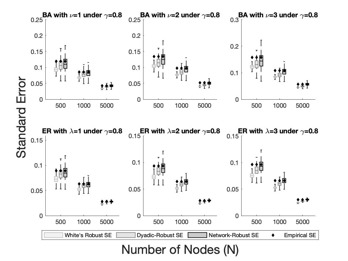
Figure 2: Boxplots of Standard Errors for Specifications 1 and 2 ($S=2$, $\gamma=0.8$)

• Note: This figure shows boxplots describing the estimated standard errors and the empirical standard errors for various combinations of parameters under Specification 1 (Barabási-Albert networks) and Specification 2 (Erdös-Renyi networks). The horizontal axis shows the number of nodes and the vertical axis represents the the standard error of the coefficient. The shaded boxes represent the 25th, 50th and 75th percentiles of estimated standard errors with the whiskers indicating the most extreme values that are not considered as outliers. The light-gray box illustrates the Eicker-Huber-White standard error, the medium-gray one the dyadic-robust standard error and the dark-gray one the network-robust standard error. The diamonds stand for the empirical standard error, defined as the standard deviation of the estimates of the regression coefficient. The estimator is considered as not covering the true standard error when the diamond is outside of the shaded area.

Table 5 describes the standard deviations of the estimated regression coefficients (what Aronow et al. (2015) calls the true standard errors) and the means of the estimated standard errors for each variance estimator. The round brackets indicate the biases of each estimate relative to the true standard error in percentage ($\%$). For instance, the Eicker-Huber-White variance estimator and the dyadic-robust variance estimator, when applied to Specification 1 with $\nu=3$, underestimate the true standard error by 21.45% and 14.14%, respectively.

Table 5: Means and Biases of the Standard Errors: $N=5000$, $S=2$, $\gamma=0.8$.

	Specification 1				Specification 2
	$\nu=1$	$\nu=2$	$\nu=3$		$\lambda=1$	$\lambda=2$	$\lambda=3$
True	0.0430	0.0518	0.0570		0.0285	0.0283	0.0302
Eicker-Huber-White	0.0337	0.0404	0.0448		0.0234	0.0229	0.0239
(Bias %)	(-21.61)	(-21.92)	(-21.45)		(-17.91)	(-19.14)	(-20.68)
Dyadic-robust	0.0403	0.0453	0.0490		0.0270	0.0266	0.0275
(Bias %)	(-6.19)	(-12.54)	(-14.14)		(-5.01)	(-6.12)	(-8.93)
Network-robust	0.0425	0.0509	0.0565		0.0280	0.0285	0.0302
(Bias %)	(-1.09)	(-1.78)	(-0.92)		(-1.70)	(0.58)	(0.09)

• Note: This table shows the standard deviations of the estimated regression coefficients (the true standard error) and the means of the estimated standard errors for each variance estimator with the round brackets indicating the biases relative to the true standard error in percentage ($\%$). To facilitate the comparison, the biases are rounded off to the second decimal places.

C.3 $S=2$ and $\gamma=0.8$ with Higher Density Parameters

This subsection examines how an increase in the number of connected dyads affects the performance of the dyadic-robust variance estimator. Table 6 reports the results for the case of $S=2$ with $\gamma=0.8$, i.e., the same combination as the main text (Table 1), but for denser networks which set $\nu=4,5$ for Specification 1 and $\lambda=4,5$ for Specification 2. We find that, while our estimator performs well (with coverage close to the nominal level), the bias in the Eicker-Huber-White and dyadic-robust estimators variance estimators are present and increase as the network becomes denser.

Table 6: The empirical coverage probability and average length of confidence intervals for $\beta$ at $95\%$ nominal level: $S=2$, $\gamma=0.8$, higher denseness parameters.

		Specification 1			Specification 2
	$N$	$\nu=4$	$\nu=5$		$\lambda=4$	$\lambda=5$
		Coverage Probability
Eicker-Huber-White	500	0.8758	0.8688		0.8744	0.8706
	1000	0.8752	0.8688		0.8694	0.8784
	5000	0.8658	0.8808		0.8694	0.8750
Dyadic-robust	500	0.8912	0.8808		0.9142	0.9058
	1000	0.8936	0.8852		0.9124	0.9160
	5000	0.8940	0.9020		0.9152	0.9176
Network-robust	500	0.9084	0.8928		0.9394	0.9368
	1000	0.9246	0.9190		0.9424	0.9494
	5000	0.9404	0.9436		0.9450	0.9512
		Average Length of the C.I.
Eicker-Huber-White	500	0.5282	0.5577		0.3088	0.3230
	1000	0.3964	0.4155		0.2183	0.2323
	5000	0.1944	0.2132		0.0992	0.1045
Dyadic-robust	500	0.5580	0.5841		0.3471	0.3601
	1000	0.4211	0.4380		0.2465	0.2595
	5000	0.2085	0.2254		0.1124	0.1172
Network-robust	500	0.6099	0.6428		0.3825	0.4022
	1000	0.4751	0.4966		0.2743	0.2927
	5000	0.2449	0.2660		0.1259	0.1331

• Note: The upper-half of the table displays the empirical coverage probability of the asymptotic confidence interval for $\beta$, and the lower-half showcases the average length of the estimated confidence intervals. As the sample size ($N$) increases, the empirical coverage probability approaches $0.95$, the nominal level. This convergence is accompanied by the shrinking average length of confidence intervals.

C.4 $S=2$ and $\gamma=0.2$

Table 7 presents the empirical coverage probability and average length of confidence intervals for $\beta$ at $5\%$ nominal size when $S=2$ and $\gamma=0.2$. The associated boxplots are given in Figure 3. Since the magnitude of spillovers is now much smaller than the case of $\gamma=0.8$, there are only minor differences in performance between the network-robust variance estimator and the other two existing methods (namely, the Eicker-Huber-White and dyadic-robust variance estimators). In terms of convergence, the comparable performance of the dyadic-robust-variance estimator is evident in Figure 3.

Comparing Table 7 to Table 1 highlights the impact of spillovers on the variance estimators. When the spillovers are substantially weak (e.g., $\gamma=0.2$), the dyadic-robust variance estimator can serve as a good substitute for the network-robust one. In the case of relatively high spillovers (e.g., $\gamma=0.8$), on the other hand, there are evident biases (around 4 percentage points for Specification 1 and 3 percentage points for Specification 2 when $N=5000$). Based on this comparison, we suggest that the network-robust variance estimator be used when the correlations are expected to be relatively strong.

Table 7: The empirical coverage probability and average length of confidence intervals for $\beta$ at $95\%$ nominal level: $S=2$, $\gamma=0.2$.

		Specification 1				Specification 2
	$N$	$\nu=1$	$\nu=2$	$\nu=3$		$\lambda=1$	$\lambda=2$	$\lambda=3$
		Coverage Probability
Eicker-Huber-White	500	0.9286	0.9186	0.9108		0.9434	0.9292	0.9308
	1000	0.9320	0.9158	0.9148		0.9338	0.9322	0.9322
	5000	0.9200	0.9110	0.9124		0.9434	0.9382	0.9308
Dyadic-robust	500	0.9342	0.9350	0.9336		0.9454	0.9368	0.9422
	1000	0.9454	0.9376	0.9458		0.9398	0.9422	0.9486
	5000	0.9446	0.9448	0.9432		0.9486	0.9490	0.9472
Network-robust	500	0.9284	0.9246	0.9162		0.9428	0.9360	0.9384
	1000	0.9414	0.9294	0.9370		0.9392	0.9410	0.9456
	5000	0.9454	0.9476	0.9418		0.9494	0.9492	0.9470
		Average Length of the Confidence Intervals
Eicker-Huber-White	500	0.1578	0.1214	0.1092		0.1860	0.1360	0.1141
	1000	0.1088	0.0846	0.0743		0.1290	0.0955	0.0799
	5000	0.0486	0.0388	0.0346		0.0579	0.0423	0.0357
Dyadic-robust	500	0.1648	0.1316	0.1213		0.1890	0.1410	0.1205
	1000	0.1158	0.0931	0.0833		0.1319	0.0994	0.0848
	5000	0.0532	0.0439	0.0398		0.0594	0.0443	0.0381
Network-robust	500	0.1637	0.1291	0.1174		0.1885	0.1404	0.1196
	1000	0.1154	0.0922	0.0825		0.1318	0.0993	0.0848
	5000	0.0533	0.0440	0.0401		0.0594	0.0444	0.0382

• Note: The upper-half of the table displays the empirical coverage probability of the asymptotic confidence interval for $\beta$, and the lower-half showcases the average length of the estimated confidence intervals. One computational issue that plagues the Monte Carlo simulation is the potential lack of positive-semi-definiteness of the estimated variance-covariance matrix. In general, this problem prevails only when the sample size ($N$) is small. In our case, when $N=500$, four variance estimates out of five thousands take negative values. We deal with this issue by first applying the eigenvalue decomposition to the estimated variance-covariance matrix and then augmenting the diagonal matrix of eigenvalues by a small constant, followed by pre- and post-multiplications by the matrix of eigenvectors to obtain the updated estimate for the variance-covariance matrix. As the sample size ($N$) increases, the empirical coverage probability approaches $0.95$, the nominal level. This convergence is accompanied by the shrinking average length of confidence intervals.

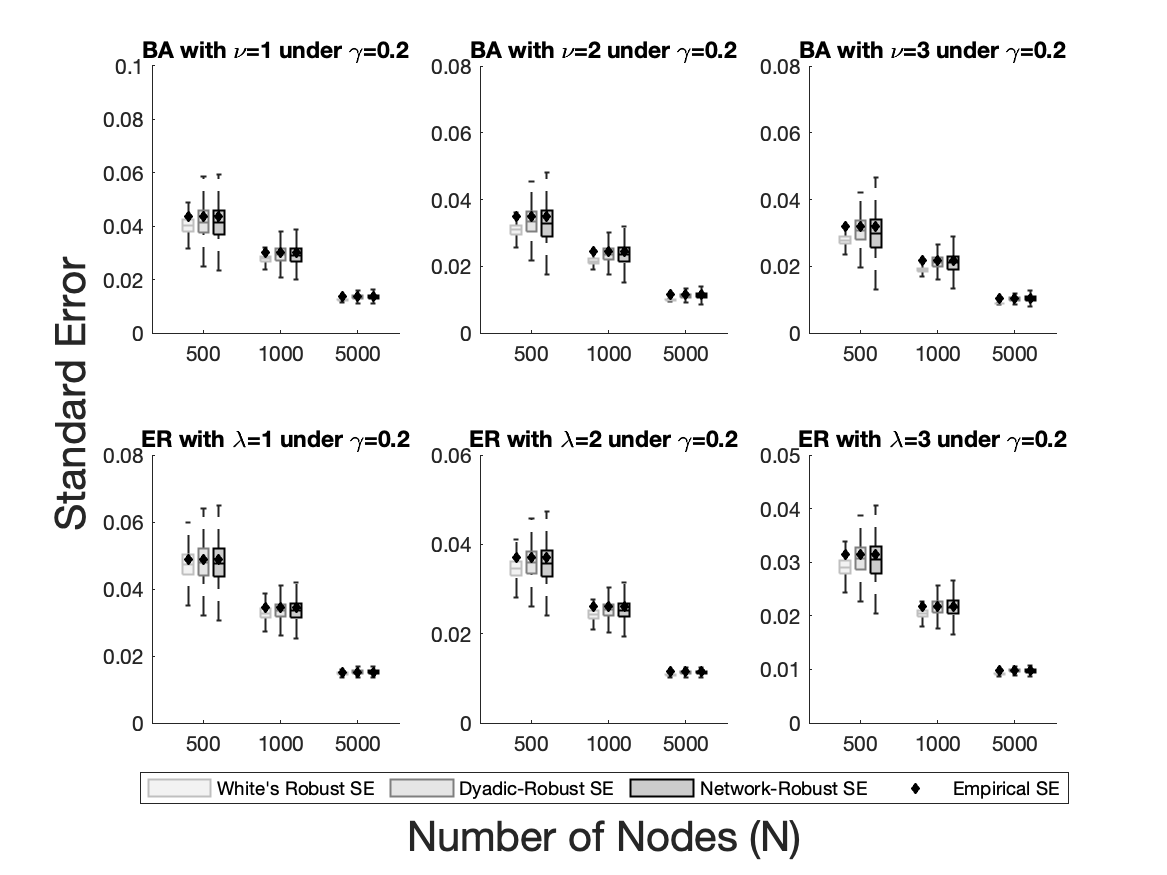
Figure 3: Boxplots of Standard Errors for Specifications 1 and 2 ($S=2$, $\gamma=0.2$)

• Note: This figure shows boxplots describing the estimated standard errors and the empirical standard errors for various combinations of parameters under Specification 1 (Barabási-Albert networks) and Specification 2 (Erdös-Renyi networks). The horizontal axis shows the number of nodes and the vertical axis represents the the standard error of the coefficient. The shaded boxes represent the 25th, 50th and 75th percentiles of estimated standard errors with the whiskers indicating the most extreme values that are not considered as outliers. The light-gray box illustrates the Eicker-Huber-White standard error, the medium-gray one the dyadic-robust standard error and the dark-gray one the network-robust standard error. The diamonds stand for the empirical standard error, defined as the standard deviation of the estimates of the regression coefficient. This figure showcases the boxplots for the case when $\gamma=0.2$.

C.5 $S=1$

For comparison purposes, this subsection explores the results for $S=1$. If $S=1$, there are no higher-order correlations beyond direct (adjacent) neighbors. Then, the network-robust variance estimator ought to coincide with the dyadic-robust variance estimator by definition, for any $\gamma$, as pointed out in Example 2.1. This is verified below for the case of $\gamma=0.8$. Table 8 shows the simulation results.

Table 8: The empirical coverage probability and average length of confidence intervals for $\beta$ at $95\%$ nominal level: $S=1$, $\gamma=0.8$.

		Specification 1				Specification 2
	$N$	$\nu=1$	$\nu=2$	$\nu=3$		$\lambda=1$	$\lambda=2$	$\lambda=3$
		Coverage Probability
Eicker-Huber-White	500	0.8804	0.8676	0.8734		0.8906	0.8768	0.8692
	1000	0.8678	0.8810	0.8710		0.8984	0.8864	0.8856
	5000	0.8752	0.8652	0.8742		0.8996	0.8910	0.8778
Dyadic-robust	500	0.9292	0.9304	0.9384		0.9366	0.9416	0.9368
	1000	0.9364	0.9426	0.9432		0.9428	0.9454	0.9484
	5000	0.9474	0.9414	0.9498		0.9452	0.9518	0.9506
Network-robust	500	0.9292	0.9304	0.9384		0.9366	0.9416	0.9368
	1000	0.9364	0.9426	0.9432		0.9428	0.9454	0.9484
	5000	0.9474	0.9414	0.9498		0.9452	0.9518	0.9506
		Average Length of the Confidence Intervals
Eicker-Huber-White	500	0.3282	0.2901	0.2881		0.2664	0.2377	0.2235
	1000	0.2321	0.2088	0.1964		0.1887	0.1665	0.1564
	5000	0.1131	0.1042	0.0980		0.0844	0.0742	0.0704
Dyadic-robust	500	0.3934	0.3591	0.3603		0.3104	0.2888	0.2776
	1000	0.2853	0.2625	0.2500		0.2227	0.2037	0.1950
	5000	0.1428	0.1330	0.1259		0.0998	0.0913	0.0882
Network-robust	500	0.3934	0.3591	0.3603		0.3104	0.2888	0.2776
	1000	0.2853	0.2625	0.2500		0.2227	0.2037	0.1950
	5000	0.1428	0.1330	0.1259		0.0998	0.0913	0.0882

• Note: The upper-half of the table displays the empirical coverage probability of the asymptotic confidence interval for $\beta$, and the lower-half showcases the average length of the estimated confidence intervals. As the sample size ($N$) increases, the empirical coverage probability approaches $0.95$, the nominal level. This convergence is accompanied by the shrinking average length of confidence intervals.

C.6 $S=\infty$ with the Parzen kernel

In this subsection, we investigate the consequences of adaptively choosing the value of the lag-truncation parameter following the rule outlined in the main text. To this end, we set $S=\infty$ (i.e., spillovers may propagate to all neighbors), with the magnitude of the spillovers controlled by $\gamma=0.8$ (the same as in the main text). In this environment, the spillovers are never truncated while decaying as they propagate farther. With regards to estimation, we consider the Parzen kernel, letting the lag-truncation parameter be chosen on the basis of Kojevnikov et al. (2021). The simulation results are given in Table 9, while the selected lag-truncation parameters are shown in Table C.6.

The empirical coverage probability based on the network-robust variance estimator approaches to 95%, as expected. On the other hand, both the Eicker-Huber-White and dyadic-robust variance estimator understate the targeted nominal level, as claimed in the main text. It should be noted that these biases can become larger when the decay rate is slower. We focus on Specification 2, as it likely satisfies the assumptions above under $S=\infty$. After all, with $S=\infty$ and a very dense network, Assumption 3.4 is violated.

Table 9: The empirical coverage probability and average length of confidence intervals for $\beta$ at $95\%$ nominal level, Specification 2: $S=\infty$, $\gamma=0.8$, the Parzen kernel.

	$N$	$\lambda=1$	$\lambda=2$	$\lambda=3$
		Coverage Probability
Eicker-Huber-White	500	0.8884	0.8768	0.8718
	1000	0.8892	0.8832	0.8806
	5000	0.8966	0.8820	0.8806
Dyadic-robust	500	0.9282	0.9150	0.8964
	1000	0.9300	0.9214	0.9126
	5000	0.9384	0.9272	0.9118
Network-robust	500	0.9366	0.9302	0.9180
	1000	0.9382	0.9386	0.9362
	5000	0.9480	0.9510	0.9462
		Average Length of C.I.
Eicker-Huber-White	500	0.2890	0.3085	0.3658
	1000	0.2103	0.2241	0.2570
	5000	0.0933	0.0994	0.1188
Dyadic-robust	500	0.3293	0.3483	0.3966
	1000	0.2405	0.2526	0.2809
	5000	0.1075	0.1127	0.1300
Network-robust	500	0.3387	0.3705	0.4233
	1000	0.2502	0.2729	0.3070
	5000	0.1120	0.1233	0.1457

• Note: The upper-half of the table displays the empirical coverage probability of the asymptotic confidence interval for $\beta$, and the lower-half showcases the average length of the estimated confidence intervals. As the sample size ($N$) increases, the empirical coverage probability approaches $0.95$, the nominal level. This convergence is accompanied by the shrinking average length of confidence intervals.

Table 10: The lag-truncation parameters for Table 9 based on the Kojevnikov_et_al-2021 rule.

$N$	$\lambda=1$	$\lambda=2$	$\lambda=3$
500	224.3186	17.5262	12.0174
1000	254.5841	20.0388	13.4822
5000	320.3268	24.1851	16.0915

Note: This table displays the lag-truncation parameters $b_{M}$ for the simulations in Table 9, selected using the rule: $b_{M}=2\log(M)/\log(\max(average~{}degree,1.05))$, with $M$ denoting the number of active dyads.

Appendix D Additional Information for the Empirical Illustration

D.1 Seating Arrangement at the European Parliament

Figure 4 exhibits an example of the seating arrangement at the European Parliament, and describes how we construct an adjacency relationship among MEPs within their EPG groups.

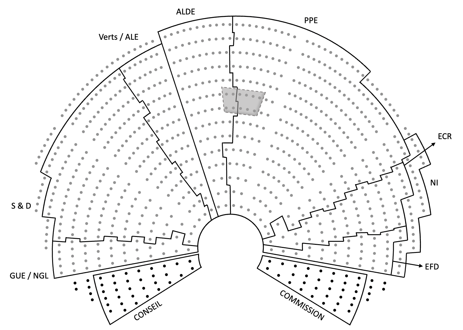
Figure 4: Seating Plan at the European Parliament: Strasbourg, September 14, 2009

ALDE PPE Row 10 $\cdots$ $\vdots$ $\vdots$ $\vdots$ $\vdots$ $\vdots$ $\vdots$ $\cdots$ Row 9 $\cdots$ Seat 36: Seat 37: Seat 38: Seat 39: Seat 40: Seat 41: $\cdots$ ALFANO ALVARO CAVADA COELHO COLLINO COMI Row 8 $\cdots$ Seat 32: Seat 33: Seat 34: Seat 35: Seat 36: $\cdots$ OJULAND OVIIR BACH BALDASSARRE BALZ Row 7 $\cdots$ $\vdots$ $\vdots$ $\vdots$ $\vdots$ $\vdots$ $\vdots$ $\cdots$

• Note: The upper panel illustrates a zoomed-out view of a seating plan for the European parliament in Strasbourg on September 14, 2009. gray circles are individual MEPs, while black circles embody members of conseil and commission. The associated party (EPG) is denoted at the top. The lower panel provides a zoomed-in view elaborating on the part of the upper panel marked by the dotted trapezoid shaded in gray. Alafano and Alvaro are treated as adjacent because they are sitting next to each other and belong to the same political party, i.e., ALE. Similarly, Ojuland and Oviir are considered to be adjacent. On the other hand, following the original authors, Alvaro and Cavada are not regarded as adjacent though they are seated together because they belong to different political parties, i.e., ALE and PPE, respectively. In terms of dyad-level adjacency, Cavada-Coelho and Coelho-Collino are adjacent dyads as they share Coelho, whereas Cavada-Coelho and Collino-Comi are not adjacent, but they are still connected as they have indirect paths to one another along the dyadic network.

D.2 Summary Statistics of the Seating Arrangement

Table 11 lists the summary statistics of the seating arrangement (for Strasbourg at term 7) when viewed as a network over pairs of MEPs. Its summary statistics are consistent with those from the Erdös-Renyi random network with $\lambda=1$ to $\lambda=3$ (see Table 4). This suggests that our empirical illustration should perform well with the Parzen kernel and bandwidth choice proposed in Kojevnikov et al. (2021).

Table 11: Summary Statistics of The Seating Arrangement: Strasbourg, Term 7

$d_{act}$	$d_{max}$	$d_{ave}$	$e_{direct}$	$e_{indirect}$
602	2	1.7076	514	3136

See Table 4 for the definition of the first three indicators. The last two represent the number of adjacent and connected dyads, respectively.

D.3 Data Construction

Data construction for our empirical exercise in Section 5 proceeds in multiple steps:

Step 1:

Our subsample consists of the location of interest (i.e., Strasbourg) for the period of interest (i.e., Term 7). We select a further subset of the extracted data by seating arrangement (i.e., we focus on Pattern 1 for the present analysis - see Table 12).

Step 2:

Since our analysis is concerned with voting concordance, we follow the original authors in dropping entries with missing data or “abstain” in the variable “vote.”

Step 3:

The resulting data still contains individuals belonging to “Identity, Tradition and Sovereignty (ITS),” one of the European Political Groups that dissolved in November 7, during the sixth term. We drop such MEPs from our analysis.

Step 4:

The selected data is used to form the dyadic data registering the pair-of-MEPs-specific information. When pairing two MEPs, we follow Harmon et al. (2019) in focusing on those pairs of MEPs, both of whom are

• in the same EPG;

• from an alphabetically-seated EPG; and

• non-leaders at the time of voting.

Our dyadic data consists of two types of variables: binary variables and numerical variables. The dyad-level binary (i.e., indicator) variables are defined to be one if the individual-level binary variables are the same, and zero otherwise. The dyadic-specific numerical variables in our analysis are the differences between the individual-level numerical variables, such as age and tenure. When calculating the differences in ages and tenures, we take the absolute values as we do not consider directional dyads, and we then rescale them into ten-year units. See the note below Table 2 for details.

Table 12: Patterns of Seating Arrangements: Strasbourg, Term 7

Pattern	Date			Number of Proposals
1	7/14/2009	$\sim$	7/16/2009	116
2	8/18/2009	$\sim$	8/21/2009	72
3	9/23/2009	$\sim$	9/25/2009	114
4	10/13/2009	$\sim$	10/16/2009	40
5	11/19/2009	$\sim$	12/11/2009	94
6	1/5/2010	$\sim$	1/8/2010	79
7	3/17/2010	$\sim$	3/19/2010	45
8	4/14/2010	$\sim$	4/16/2010	120
9	5/5/2010	$\sim$	5/7/2010	79
10	7/7/2010	$\sim$	7/9/2010	34
11	7/21/2010	$\sim$	7/22/2010	50
12	8/18/2010	$\sim$	8/20/2010	118

• Note: This table presents patterns of seating arrangements with the corresponding dates and the number of total observations for each pattern. Since voting may be taken place for multiple proposals within the same day, the total number proposals tends to be higher than that of days in a single pattern. For example, the first line indicates that 116 proposals were discussed and votes were cast over the three days (from the 14th of July, 2009 to the 16th of July, 2009).

D.4 Full Results

Table 13 reports the detailed result of the empirical illustration. As explained in Section 5.3, Panel A reports the estimates of the parameter of interest, while Panel B lists the standard errors based on the different variance estimators. In particular, we carry out the estimation using both the network-robust variance estimator with the mean-shifted rectangular kernel, and the one with the Parzen kernel, generating the same estimates. Panel C collects the parameter estimates for other covariates accompanied by the standard errors obtained from our proposed variance estimator from equation (10), and indicates the presence or absence of day-level fixed effects.

Table 13: Spillovers in Legislative Voting – Main Analysis

	Specification (I)	Specification (II)	Specification (III)
Panel A: Parameter estimates for Seat neighbors
Seat neighbors	0.0069	0.0060	0.0060
Panel B: Standard errors for Seat neighbors
Eicker-Huber-White	0.0031	0.0030	0.0030
Dyadic-robust	0.0075	0.0082	0.0087
Network-robust (with the rectangular kernel)	0.0095	0.0104	0.0112
Network-robust (with the Parzen kernel)	0.0095	0.0104	0.0112
Panel C: Parameter estimates for other covariates
Same country		0.0561	0.0562
		(0.0008)	(0.0008)
Same quality education		0.0030	0.0028
		(0.0007)	(0.0007)
Same freshman status		-0.0070	-0.0070
		(0.0008)	(0.0008)
Same gender		0.0004	0.0004
		(0.0007)	(0.0006)
Age difference		0.0007	0.0004
		(0.0004)	(0.0004)
Tenure difference		-0.0149	-0.0149
		(0.0006)	(0.0006)
Day-level FE	No	No	Yes

• Note: Panel A displays the parameter estimates for the three different specifications; Panel B shows the standard errors for the regression coefficient of SeatNeighbors using different variance estimators; and Panel C collects the parameter estimates for other covariates accompanied by the standard errors obtained from our proposed variance estimator from equation (10), and indicates the presence or absence of day-level fixed effects. Adjacency of MEPs is defined at the level of a row-by-EP-by-EPG. (See the note below Figure 4.) Independent variables are as follows: Seat neighbors is an indicator variable denoting whether both MEPs sit together; Same country represents an indicator for whether both MEPs are from the same country; Same quality education is an indicator showing whether both MEPs have the same quality of education background, measured by if both have the degree from top 500 universities; Same freshman status encodes whether both MEPs are freshman or not; Age difference is the difference in the MEPs’ ages; and Tenure difference measures the difference in the MEPs’ tenures.

References

- Abadie et al. (2022) Abadie, A., S. Athey, G. W. Imbens, and J. M. Wooldridge (2022). When should you adjust standard errors for clustering? The Quarterly Journal of Economics Forthcoming.
- Acemoglu et al. (2015) Acemoglu, D., C. García-Jimeno, and J. A. Robinson (2015). State capacity and economic development: A network approach. American Economic Review 105(8), 2364–2409.
- Anderson and van Wincoop (2003) Anderson, J. E. and E. van Wincoop (2003). Gravity with gravitas: A solution to the border puzzle. American Economic Review 93(1), 170–192.
- Aronow et al. (2015) Aronow, P. M., C. Samii, and V. A. Assenova (2015). Cluster–robust variance estimation for dyadic data. Political Analysis 23(4), 564–577.
- Barabási and Albert (1999) Barabási, A. L. and R. Albert (1999). Emergence of scaling in random networks. Science 286(5439), 509–512.
- Bliss and Russett (1998) Bliss, H. and B. Russett (1998). Democratic trading partners: The liberal connection, 1962-1989. The Journal of Politics 60(4), 1126–1147.
- Cameron et al. (2011) Cameron, A. C., J. B. Gelbach, and D. L. Miller (2011). Robust inference with multiway clustering. Journal of Business & Economic Statistics 29(2), 238–249.
- Cameron and Miller (2014) Cameron, A. C. and D. L. Miller (2014). Robust inference for dyadic data. Working Paper.
- Canen et al. (2020) Canen, N., J. Schwartz, and K. Song (2020). Estimating local interactions among many agents who observe their neighbors. Quantitative Economics 11(1), 917–956.
- Chiang et al. (2022) Chiang, H. D., B. E. Hansen, and Y. Sasaki (2022). Standard errors for two-way clustering with serially correlated time effects. Working Paper.
- Chiang et al. (2021) Chiang, H. D., K. Kato, Y. Ma, and Y. Sasaki (2021). Multiway cluster robust double/debiased machine learning. Journal of Business & Economic Statistics 40(3), 1–11.
- Chiang et al. (2022) Chiang, H. D., Y. Matsushita, and T. Otsu (2022). Multiway empirical likelihood. Working Paper.
- Chiang and Tan (2022) Chiang, H. D. and B. Y. Tan (2022). Empirical likelihood and uniform convergence rates for dyadic kernel density estimation. Journal of Business & Economic Statistics (Forthcoming), 1–9.
- Conley (1999) Conley, T. G. (1999). GMM estimation with cross sectional dependence. Journal of Econometrics 92(1), 1–45.
- Cranmer and Desmarais (2016) Cranmer, S. J. and B. A. Desmarais (2016). A critique of dyadic design. International Studies Quarterly 60(2), 355–362.
- Davezies et al. (2021) Davezies, L., X. D’Haultfœuille, and Y. Guyonvarch (2021). Empirical process results for exchangeable arrays. The Annals of Statistics 49(2), 845–862.
- de Paula et al. (2018) de Paula, A., S. Richards-Shubik, and E. Tamer (2018). Identifying preferences in networks with bounded degree. Econometrica 86(1), 263–288.
- Eaton and Kortum (2002) Eaton, J. and S. Kortum (2002). Technology, geography, and trade. Econometrica 70(5), 1741–1779.
- Erdös and Rényi (1959) Erdös, P. and A. Rényi (1959). On random graphs i. Publicationes Mathematicae 6, 290–297.
- Erdös and Rényi (1960) Erdös, P. and A. Rényi (1960). On the evolution of random graphs. Publications of the Mathematical Institute of the Hungarian Academy of Sciences 5, 17–61.
- Erikson et al. (2014) Erikson, R. S., P. M. Pinto, K. T. Rader, et al. (2014). Dyadic analysis in international relations: A cautionary tale. Political Analysis 22(4), 457–463.
- Gowa and Kim (2005) Gowa, J. and S. Y. Kim (2005). An exclusive country club: The effects of the gatt on trade, 1950–94. World Politics 57(4), 453–478.
- Graham (2020a) Graham, B. S. (2020a). Dyadic regression. In B. Graham and Á. d. Paula (Eds.), The Econometric Analysis of Network Data (1st ed.)., Chapter 2, pp. 23–40. Academic Press.
- Graham (2020b) Graham, B. S. (2020b). Network data. In S. N. Durlauf, L. P. Hansen, J. J. Heckman, and R. L. Matzkin (Eds.), Handbook of Econometrics, Volume 7A, Volume 7 of Handbook of Econometrics, Chapter 2, pp. 111–218. Elsevier.
- Graham et al. (2022) Graham, B. S., F. Niu, and J. L. Powell (2022). Kernel density estimation for undirected dyadic data. Working Paper.
- Hansen and Lee (2019) Hansen, B. E. and S. Lee (2019). Asymptotic theory for clustered samples. Journal of Econometrics 210(2), 268–290.
- Harmon et al. (2019) Harmon, N., R. Fisman, and E. Kamenica (2019). Peer effects in legislative voting. American Economic Journal: Applied Economics 11(4), 156–80.
- Helpman et al. (2008) Helpman, E., M. Melitz, and Y. Rubinstein (2008). Estimating trade flows: Trading partners and trading volumes. The Quarterly Journal of Economics 123(2), 441–487.
- Hoff and Ward (2004) Hoff, P. D. and M. D. Ward (2004). Modeling dependencies in international relations networks. Political Analysis 12(2), 160–175.
- Ibragimov and Müller (2010) Ibragimov, R. and U. K. Müller (2010). t-statistic based correlation and heterogeneity robust inference. Journal of Business & Economic Statistics 28(4), 453–468.
- Jenish and Prucha (2009) Jenish, N. and I. R. Prucha (2009). Central limit theorems and uniform laws of large numbers for arrays of random fields. Journal of Econometrics 150(1), 86–98.
- Kelejian and Prucha (2010) Kelejian, H. H. and I. R. Prucha (2010). Specification and estimation of spatial autoregressive models with autoregressive and heteroskedastic disturbances. Journal of Econometrics 157(1), 53–67.
- Kojevnikov et al. (2021) Kojevnikov, D., V. Marmer, and K. Song (2021). Limit theorems for network dependent random variables. Journal of Econometrics 222(2), 882–908.
- Leung (2021) Leung, M. P. (2021). Network cluster-robust inference. Working Paper.
- Leung (2022) Leung, M. P. (2022). Causal inference under approximate neighborhood interference. Econometrica 90(1), 267–293.
- Leung and Moon (2021) Leung, M. P. and H. R. Moon (2021). Normal approximation in large network models. Working Paper.
- Lowe and Jo (2021) Lowe, M. and D. Jo (2021). Legislature integration and bipartisanship: A natural experiment in iceland. CESifo Working Paper.
- Lustig and Richmond (2020) Lustig, H. and R. J. Richmond (2020). Gravity in the exchange rate factor structure. The Review of Financial Studies 33(8), 3492–3540.
- MacKinnon et al. (2022a) MacKinnon, J. G., M. Ø. Nielsen, and M. D. Webb (2022a). Cluster-robust inference: A guide to empirical practice. Journal of Econometrics (Forthcoming).
- MacKinnon et al. (2022b) MacKinnon, J. G., M. Ø. Nielsen, and M. D. Webb (2022b). Fast and reliable jackknife and bootstrap methods for cluster-robust inference. Working Paper.
- MacKinnon et al. (2022c) MacKinnon, J. G., M. Ø. Nielsen, and M. D. Webb (2022c). Leverage, influence, and the jackknife in clustered regression models: Reliable inference using summclust. Working Paper.
- Mansfield et al. (2000) Mansfield, E. D., H. V. Milner, and B. P. Rosendorff (2000). Free to trade: Democracies, autocracies, and international trade. American political science review 94(2), 305–321.
- Melitz (2003) Melitz, M. J. (2003). The impact of trade on intra-industry reallocations and aggregate industry productivity. Econometrica 71(6), 1695–1725.
- Menzel (2021) Menzel, K. (2021). Bootstrap with cluster-dependence in two or more dimensions. Econometrica 89(5), 2143–2188.
- Minhas et al. (2022) Minhas, S., C. Dorff, M. B. Gallop, M. Foster, H. Liu, J. Tellez, and M. D. Ward (2022). Taking dyads seriously. Political Science Research and Methods 10(4), 703–721.
- Minhas et al. (2019) Minhas, S., P. D. Hoff, and M. D. Ward (2019). Inferential approaches for network analysis: Amen for latent factor models. Political Analysis 27(2), 208–222.
- Penrose and Yukich (2003) Penrose, M. D. and J. E. Yukich (2003). Weak laws of large numbers in geometric probability. Annals of Applied Probability 13(1), 277–303.
- Poast (2016) Poast, P. (2016). Dyads are dead, long live dyads! the limits of dyadic designs in international relations research. International Studies Quarterly 60(2), 369–374.
- Saia (2018) Saia, A. (2018). Random interactions in the chamber: Legislators’ behavior and political distance. Journal of Public Economics 164, 225–240.
- Tabord-Meehan (2019) Tabord-Meehan, M. (2019). Inference with dyadic data: Asymptotic behavior of the dyadic-robust t-statistic. Journal of Business & Economic Statistics 37(4), 671–680.
- Vainora (2020) Vainora, J. (2020). Network dependence. Working Paper.