On the unramified Eisenstein spectrum

Abstract

For a split reductive group ${}^{\raisebox{2.0pt}{{\tiny{L}}}}\mathsf{G}$ over a global field, we determine the spectrum of the spherical Hecke algebra coming from the unramified Eisenstein series for the minimal parabolic ${}^{\raisebox{2.0pt}{{\tiny{L}}}}\mathsf{B}$. This is done using a certain decomposition of the Springer stack $T^{*}(\mathsf{B}\backslash\mathsf{G}/\mathsf{B})$ for the Langlands dual group $\mathsf{G}$ in the additive group of cobordisms of cohomologically proper derived quotient stacks.

1 Introduction

1.1 The automorphic form setup

1.1.1

While the main idea explored in this paper may be generalized in a multitude of directions, some of its key features are already very interesting in the following most basic situation. Further generalizations will be discussed in [16], see also Section 1.3 below.

1.1.2

We denote by $\mathbb{F}$, $\mathbb{A}$, and $\mathbb{I}$ a global field, its adeles, and ideles, respectively. We consider a split reductive group over $\mathbb{F}$, which we denote ${}^{\raisebox{2.0pt}{{\tiny{L}}}}\mathsf{G}$ because the bulk of our computations will be with the Langlands dual complex reductive group $\mathsf{G}$. On both sides, we denote by the letters $\mathsf{A}$, $\mathsf{B}$, and $\mathsf{U}$ (resp. ${}^{\raisebox{2.0pt}{{\tiny{L}}}}\mathsf{A},{}^{\raisebox{2.0pt}{{\tiny{L}}}}\mathsf{B},{}^{\raisebox{2.0pt}{{\tiny{L}}}}\mathsf{U}$) a maximal torus, a Borel subgroup containing it, and its unipotent radical. We have

$$\mathsf{A}=\Lambda\otimes_{\mathbb{Z}}\mathbb{C}^{\times}\,,\quad{}^{\raisebox{2.0pt}{{\tiny{L}}}}\mathsf{A}=\Lambda^{\vee}\!\otimes_{\mathbb{Z}}\mathbb{G}_{\mathbf{m}}\,,$$

for pair of dual lattices $\Lambda$ and $\Lambda^{\vee}$.

1.1.3

Let $\mathscr{Q}_{\mathbb{F}}\subset\mathbb{R}_{>0}$ denote the image of the norm map $\mathbb{I}\to\mathbb{R}_{>0}$. We have

$$\mathscr{Q}_{\mathbb{F}}=\begin{cases}q^{\mathbb{Z}}\,,&\mathbb{F}=\Bbbk(\textup{curve})\,,|\Bbbk|=q\,,\\ \mathbb{R}_{>0}\,,&\operatorname{char}\mathbb{F}=0\,.\end{cases}$$

For uniformity in formulas, one should interpret $q>1$ as the generator of this group, including the infinitesimal generator $t\frac{d}{dt}\in\operatorname{Lie}\mathbb{R}_{>0}$, in the number field case.

We have the dual map

$$\mathbb{C}\cong\operatorname{Hom}(\mathbb{R}_{>0},\mathbb{C}^{\times})\to\operatorname{Hom}(\mathscr{Q}_{\mathbb{F}},\mathbb{C}^{\times})\overset{\textup{\tiny def}}{=}\mathscr{Q}_{\mathbb{F}}^{\vee}\,,$$

where the first isomorphism sends $t\in\mathbb{R}_{>0}$ to $t^{s}$, $s\in\mathbb{C}$. In other words,

$$\mathscr{Q}_{\mathbb{F}}^{\vee}=\begin{cases}\mathbb{C}\left/\frac{2\pi i}{\ln q}\,\mathbb{Z}\right.\,,&\operatorname{char}\mathbb{F}>0\,,\\ \mathbb{C}\,,&\operatorname{char}\mathbb{F}=0\,.\end{cases}$$ (1)

In both cases we have a well-defined map

$$\Re:\mathscr{Q}_{\mathbb{F}}^{\vee}\to\mathbb{R}\,.$$

1.1.4

The characters of ${}^{\raisebox{2.0pt}{{\tiny{L}}}}\mathsf{A}(\mathbb{A})$ that factor through the norm map

(2)

are parametrized by

$$\lambda\in\Lambda\otimes\mathscr{Q}_{\mathbb{F}}^{\vee}\cong\begin{cases}\mathsf{A}\,,&\operatorname{char}\mathbb{F}>0\,,\\ \operatorname{Lie}\mathsf{A}\,,&\operatorname{char}\mathbb{F}=0\,.\end{cases}$$

Given such $\lambda$, one defines the Eisenstein series

$$E(\lambda,g)=\sum_{\gamma\in{}^{\raisebox{2.0pt}{{\tiny{L}}}}\mathsf{G}(\mathbb{F})/{}^{\raisebox{2.0pt}{{\tiny{L}}}}\mathsf{B}(\mathbb{F})}\|a(g\gamma)\|^{\lambda+\rho}\,,$$ (3)

where $a(g)\in{}^{\raisebox{2.0pt}{{\tiny{L}}}}\mathsf{A}$ is the torus part in the Iwasawa ${}^{\raisebox{2.0pt}{{\tiny{L}}}}\mathsf{K}{}^{\raisebox{2.0pt}{{\tiny{L}}}}\mathsf{A}{}^{\raisebox{2.0pt}{{\tiny{L}}}}\mathsf{U}$ decomposition of $g$, and $\rho\in\Lambda$ is the half sum of the roots in ${}^{\raisebox{2.0pt}{{\tiny{L}}}}\mathsf{B}$. The series (3) converges for $\Re\lambda$ inside the positive cone of $\Lambda\otimes\mathbb{R}$, which we express by the notation $\Re\lambda>0$.

1.1.5

More generally, given a function

$$\phi^{\vee}:\Lambda^{\vee}\otimes\mathscr{Q}_{\mathbb{F}}\to\mathbb{C}$$

with compact support, one may consider the corresponding pseudo-Eisenstein series

$$E_{\phi^{\vee}}(g)=\sum_{\gamma\in{}^{\raisebox{2.0pt}{{\tiny{L}}}}\mathsf{G}(\mathbb{F})/{}^{\raisebox{2.0pt}{{\tiny{L}}}}\mathsf{B}(\mathbb{F})}\phi^{\vee}(\|a(g\gamma)\|)\,.$$ (4)

The series (3) and (4) are related by the Mellin transform on the group $\Lambda^{\vee}\otimes\mathscr{Q}_{\mathbb{F}}$. If $\phi$ is a function on $\Lambda\otimes\mathscr{Q}_{\mathbb{F}}^{\vee}$ which is the Mellin transform of $\phi^{\vee}$ then

$$E_{\phi^{\vee}}(g)=\int_{\Re\lambda=\lambda_{0}\gg 0}E(\lambda,g)\phi(\lambda)d\lambda\,.$$

1.1.6

The following fundamental result is due to R. Langlands

Theorem 1 ([L]).

The Hermitian product

$$(f_{1},f_{2})_{\textup{Eis}}\overset{\textup{\tiny def}}{=}(E_{f_{1}^{\vee}},E_{f_{1}^{\vee}})_{L^{2}\left({}^{\raisebox{2.0pt}{{\tiny{L}}}}\mathsf{G}(\mathbb{A})\,/\,{}^{\raisebox{2.0pt}{{\tiny{L}}}}\mathsf{G}(\mathbb{F})\right)}$$ (5)

is given by the following formula

$$(f_{1},f_{2})_{\textup{Eis}}=\int_{\Re\lambda=\lambda_{0}\gg 0}d\lambda\sum_{w\in W}f_{1}(\lambda)\,\overline{f_{2}}(-w\cdot\lambda)\!\!\prod_{\begin{subarray}{c}\alpha>0\\ w\cdot\alpha<0\end{subarray}}\frac{\xi_{\mathbb{F}}(\alpha(\lambda))}{\xi_{\mathbb{F}}(1+\alpha(\lambda))}\,,$$ (6)

where $\overline{f}(x)=\overline{f(\overline{x})}$, $\{\alpha\}$ are the roots of $\mathsf{G}$, and $\xi(x)$ is the completed $\zeta$-function of $\mathbb{F}$.

The summation over $W$ in (6) comes from the Bruhat decomposition of the group ${}^{\raisebox{2.0pt}{{\tiny{L}}}}\mathsf{G}(\mathbb{F})$ and the ratios of $\zeta$-functions appear as the spherical matrix elements of intertwining operators associated to $w\in W$. See Appendix A.4 for a discussion of the normalization of the Lebesgue measure in (6).

1.1.7

Our object of interest in this paper is

$$\mathscr{H}_{\textup{Eis}}=\overline{\operatorname{span}\left\{E_{\phi^{\vee}}(g)\right\}}\subset L^{2}\!\left(\,{}^{\raisebox{2.0pt}{{\tiny{L}}}}\mathsf{G}(\mathbb{A})\,\big{/}\,{}^{\raisebox{2.0pt}{{\tiny{L}}}}\mathsf{G}(\mathbb{F})\right)\,.$$ (7)

This is a Hilbert space with an action of a large commutative $*$-algebra generated by the spherical Hecke operators at all nonarchimedian places (and also invariant differential operators at Archimedean places). Since Eisenstein series are joint eigenfunctions of all these operators, we may realize a dense (in the sense of having the same commutant) subalgebra $\mathbf{sH}$ of this algebra concretely as

$$\mathbf{sH} =\textup{$W$-invariant functions of $\lambda$}$$

$$=\mathbb{C}\left[\underline{\mathsf{A}}\,/\,W\right]\,,$$ (8)

where

$$\underline{\mathsf{A}}=\Lambda\otimes\mathscr{Q}_{\mathbb{F}}^{\vee}\cong\begin{cases}\mathsf{A}\,,&\operatorname{char}\mathbb{F}>0\,,\\ \operatorname{Lie}\mathsf{A}\,,&\operatorname{char}\mathbb{F}=0\,.\end{cases}$$ (9)

The problem that we solve in this paper is to determine the spectrum of $\mathbf{sH}$ in $\mathscr{H}_{\textup{Eis}}$.

1.1.8

As envisioned by Langlands, $\mathscr{H}_{\textup{Eis}}$ breaks up into a direct sum, the pieces in which are indexed by the conjugacy classes of nilpotent elements $e\in\mathfrak{g}=\operatorname{Lie}\mathsf{G}$. Here $\mathsf{G}$ is the Langlands dual group.

Recall that there are only finitely many conjugacy classes of nilpotent elements in $\mathfrak{g}$. Further, by the Jacobson-Morozov theorem, every $e$ has the form

$$e=\phi\left(\begin{bmatrix}0&1\\ 0&0\end{bmatrix}\right)$$ (10)

for a homomorphism $\phi:\mathfrak{sl}_{2}\to\mathfrak{g}$. The element

$$h=\phi\left(\begin{bmatrix}1&0\\ 0&-1\end{bmatrix}\right)\,,$$ (11)

known as the characteristic of $e$, satisfies

$$[h,e]=2e\,.$$

Note this includes the case

$$(e,h)=(0,0)$$

which corresponds to $\phi=0$. The nilpotent element $e$ and its characteristic $h$ determine each other up to the action of the respective centralizers.

We denote by

$$\mathsf{C}_{e}\supset\mathsf{C}_{\phi}$$

the centralizers of $e$ and of the pair $\{e,h\}$. The group $\mathsf{C}_{\phi}$ is reductive and is a maximal reductive subgroup of $\mathsf{C}_{e}$. We denote by $\mathsf{C}_{\phi,\textup{cmp}}\subset\mathsf{C}_{\phi}$ a maximal compact subgroup. It is also a maximal compact subgroup of $\mathsf{C}_{e}$.

1.1.9

Given $\phi$, we define

$$\widetilde{\mathbf{S}}_{e}=\begin{cases}q^{h/2}\mathsf{C}_{\phi,\textup{cmp}}\,,&\operatorname{char}\mathbb{F}>0\,,\\ \frac{1}{2}h+\operatorname{Lie}\mathsf{C}_{\phi,\textup{cmp}}\,,&\operatorname{char}\mathbb{F}=0\,.\end{cases}$$ (12)

These subsets of $\mathsf{G}$, resp. $\operatorname{Lie}\mathsf{G}$, are determined by $e$ up-to conjugation. Since

$$\underline{\mathsf{A}}\,/\,W=\textup{conjugacy classes of semisimple elements in}\begin{cases}\mathsf{G}\,,&\operatorname{char}\mathbb{F}>0\,,\\ \operatorname{Lie}\mathsf{G}\,,&\operatorname{char}\mathbb{F}=0\,,\end{cases}$$

we have a well-defined real-algebraic subvariety

$$\mathbf{S}_{e}=\textup{Image}\left(\widetilde{\mathbf{S}}_{e}\to\underline{\mathsf{A}}\,/\,W\right)\,.$$ (13)

We equip $\mathbf{S}_{e}$ with the push-forward of the Haar measure $d_{\textup{Haar}}$ from $\widetilde{\mathbf{S}}_{e}$, which we denote by the same symbol.

1.1.10

The following is our main result. The represents the next step in a very long development of the subject, see in particular [MW, Labesse] for a discussion of prior results.

Theorem 2.

We have the decomposition

$$\mathscr{H}_{\textup{Eis}}=\bigoplus_{e}L^{2}\left(\mathbf{S}_{e},\boldsymbol{\mu}_{e}\right)\,,$$ (14)

consistent with the inclusion $\mathsf{S}_{e}\subset\operatorname{Spec}\mathbf{sH}$, where $\boldsymbol{\mu}_{e}$ is a measure with a density with respect to $d_{\textup{Haar}}$.

We also give an explicit formula for spectral projectors and for the measure $\boldsymbol{\mu}_{e}$, see Theorem 5. The proof of Theorem 2 is completed in Section 4.4.

1.2 Large-scale structure of the argument

1.2.1

In his fundamental work [L], R. Langlands introduced a contour shift and the analysis of residues as a way to describe the discrete spectrum of $\mathscr{H}_{\textup{Eis}}$ as an $\mathbf{sH}$ -module. In [L], he computed the discrete spectrum for groups for groups of rank 2. In the work [Moe1, Moe2] of C. Mœglin and J.-L. Waldspurger this approach was used to describe the discrete spectrum of $\mathscr{H}_{\textup{Eis}}$ for all classical group. In recent work of Volker Heiermann, Marcelo de Martino and Eric Opdam [13] this approach was extended to general split groups, in the number field case (computer aided in the exceptional cases). The most recent progress will be reflected in a new version of [13], currently in preparation.

In this paper, we do something rather different, and our starting point is the following geometric interpretation of the pairing (6). In an equivalent and slightly more convenient language, we will start with a geometric interpretation of the linear functional, or distribution, $\Psi_{\textup{Eis}}$ defined by

$$(f_{1},f_{2})_{\textup{Eis}}=(f_{1}\boxtimes f_{2}^{*},\Psi_{\textup{Eis}})\,.$$ (15)

Here

$$f^{*}(\lambda)=\overline{f}(-\lambda)\,,\quad\lambda\in\underline{\mathsf{A}}\,,$$

where minus refers to the group structure of $\underline{\mathsf{A}}$. See Section 2.1.6 for a discussion of what we mean by distributions in this paper.

1.2.2

Recall the group $\mathscr{Q}_{\mathbb{F}}^{\vee}$ defined in (1) and note this is a 1-dimensional connected affine algebraic group over $\mathbb{C}$. To such an object one can associate an equivariant complex-oriented cohomology theory. This is contravariant a functor that we denote by

$$\begin{matrix}\textup{topological spaces}\\ \textup{with an action of}\\ \textup{a compact group}\end{matrix}\quad\xrightarrow{\quad{H}^{\raisebox{1.42262pt}{$\scriptscriptstyle\bullet$}}_{\textup{group}}\left(\textup{space}\big{|}\,\mathscr{Q}_{\mathbb{F}}^{\vee}\right)\quad}\quad\begin{matrix}\textup{supercommutative}\\ \textup{algebras over $\mathbb{C}$}\end{matrix}\quad.$$ (16)

Concretely, this is ordinary equivariant cohomology if $\operatorname{char}\mathbb{F}=0$ and equivariant topological K-theory if $\operatorname{char}\mathbb{F}>0$.

In particular, we have

$$\underline{\mathsf{A}}=\operatorname{Spec}{H}^{\raisebox{1.42262pt}{$\scriptscriptstyle\bullet$}}_{\mathsf{A}_{\textup{cmp}}}\left(\operatorname{pt}\big{|}\,\mathscr{Q}_{\mathbb{F}}^{\vee}\right)\,,$$ (17)

where $\underline{\mathsf{A}}$ was defined in (9) and $\mathsf{A}_{\textup{cmp}}\subset\mathsf{A}$ is the compact torus.

1.2.3

While there is a fundamental unity between equivariant K-theory and equivariant cohomology, there are also differences in details. To avoid considering cases all the time and to streamline the exposition, we will focus on the more difficult case of K-theory, the group law for which we write multiplicatively. Equivariant cohomology we treat as the $q\downarrow 1$ limit, in which we substitute

$$x_{\textup{old}}=q^{x_{\textup{new}}}$$

for all other variables, see Section 2.7 for details. In practice, this amounts to the following instruction:

1. replace the multiplicative group law by the additive group law,

2. replace $1$ by $0$, $q$ by $1$, and $1-x^{-1}$ by $x$,

3. define $\psi_{\textup{new}}(s)=\lim_{q\to 1}\psi_{\textup{old}}(q^{s};q)$, where $q^{s}$ is the argument of $\psi_{\textup{old}}$ and $q$ is a parameter on which $\psi_{\textup{old}}$ is allowed to depend.

see Table 1 in Section 2.7 for more on this.

1.2.4

The cohomology theory (16) has pushforwards for proper equivariant complex oriented maps

$$f:\mathsf{X}\to\mathsf{Y}\,.$$

For instance, if $f$ is a holomorphic map between complex manifolds, then $f$ is automatically complex oriented. As long as $f$ is proper, this setup can be extended without difficulty to suitable maps between complex algebraic stacks, as we recall in Section 2 below.

In particular, if $f$ is a proper $\mathsf{A}$-equivariant map and $\mathsf{Y}$ is a point then $f_{*}$ takes values in polynomial function on $\underline{\mathsf{A}}$. Remarkably, if one weakens the properness assumptions to cohomological properness, which is a notion recalled from [12] in Appendix A.2, then $f_{*}$ is still defined with values in distributions on $\underline{\mathsf{A}}$. This is completely analogous to the fact that the character of an infinite-dimensional representation, when defined, is typically a distribution on the group rather than a function.

The geometric interpretation of the distribution $\Psi_{\textup{Eis}}$ will be in these terms. Namely, the distribution $\Psi_{\textup{Eis}}$ on $\underline{\mathsf{A}}\times\underline{\mathsf{A}}$ will be interpreted as the pushforward under the horizontal map in

(18)

of a certain equivariant genus $\psi$ related to the completed $\zeta$-function $\xi_{\mathbb{F}}(s)$ of the field $\mathbb{F}$. See (21) below for the definition of $\mathscr{T}$.

1.2.5

As we recall in Section 2 below, genera are usually considered for either smooth compact stably complex manifolds or smooth proper algebraic varieties and involve the choice of an arbitrary function $\psi(x)\in\mathbb{C}\left[\mathscr{Q}_{\mathbb{F}}^{\vee}\right]$, such that

$$\psi(\textup{origin})=1\,.$$ (19)

If we think of argument $x$ as the equivariant Chern class of a line bundle, then the origin corresponds to a trivial line bundle.

For manifolds with an action of a group $\mathsf{A}$, genera give ring homomorphisms

$$\left\{\begin{matrix}\textup{$\mathsf{A}$-equivariant}\\ \textup{bordism classes $[\mathsf{X}]$}\end{matrix}\right\}\xrightarrow{\quad\psi(\mathsf{X})\quad}\mathbb{C}[\underline{\mathsf{A}}]\,,$$ (20)

given by

$$\psi(\mathsf{X})=(\mathsf{X}\to\operatorname{pt})_{*}\,\psi(T\mathsf{X})\,.$$

Here

$$\psi(\textup{a vector bundle $V$})=\prod_{\textup{Chern roots $v_{i}$}}\psi(v_{i})\in{H}^{\raisebox{1.42262pt}{$\scriptscriptstyle\bullet$}}_{\mathsf{A}}\left(\mathsf{X}\big{|}\,\mathscr{Q}_{\mathbb{F}}^{\vee}\right)\,.$$

This may by extended by continuity to much larger classes of functions $\psi(x)$, see Section 2.2.6. Also, the condition (19) may be relaxed if we work with manifolds of a given dimension, or stacks of given virtual dimension.

1.2.6

We define the Springer stack as

$$\mathscr{T}=T^{*}(\mathsf{B}\backslash\mathsf{G}/\mathsf{B})\,,$$ (21)

see Section 3, and give it an action of the group $\mathbb{C}^{\times}$ scaling cotangent directions with weight $-1$. The element of this multiplicative group $\mathbb{C}^{\times}$ will be denoted by $q$. We will eventually evaluate it to a prime power in the function field case. In the number field case, we will take $1\in\operatorname{Lie}\mathbb{C}^{\times}$ as a distinguished element, as already mentioned in Section 1.2.3.

Since $\mathscr{T}$ is presented as a quotient by $\mathsf{B}\times\mathsf{B}$, it comes equipped with diagonal map in (18).

1.2.7

The starting point of our analysis is the following reformulation of (6).

Theorem 3.

The stack $\mathscr{T}$ is cohomologically proper and

$$\Psi_{\textup{Eis}}=\psi_{\mathbb{F}}(\mathscr{T})\,,\quad\mathscr{T}=T^{*}(\mathsf{B}\backslash\mathsf{G}/\mathsf{B})\,,$$ (22)

where the function $\psi_{\mathbb{F}}(x)$ satisfies the equation

$$\xi_{\mathbb{F}}(s)=\begin{cases}\dfrac{\psi_{\mathbb{F}}(q^{-s})\psi_{\mathbb{F}}(q^{-1+s})}{(1-q^{s})(1-q^{1-s})}\,,&\mathscr{Q}_{\mathbb{F}}=q^{\mathbb{Z}}\,,\vspace{3mm}\\ \dfrac{\psi_{\mathbb{F}}(-s)\psi_{\mathbb{F}}(-1+s)}{s(1-s)}\,,&\operatorname{char}\mathbb{F}=0\,.\end{cases}$$ (23)

Note that since the zeros and poles of $\xi_{\mathbb{F}}(s)$ are symmetric with respect to $s\mapsto 1-s$, a function $\psi_{\mathbb{F}}(x)$ solving these equations can always be found by the Weierstraß factorization theorem.

For instance, in the function field case, we have

$$\zeta_{\mathbb{F}}(x)=\frac{\prod_{i=1}^{g}(1-\alpha_{i}/x)(1-\alpha_{i}^{-1}q/x)}{(1-1/x)(1-q/x)}\,,$$ (24)

where we use the variable $x=q^{s}$ instead of the more conventional $t=q^{-s}$, and where $\{\alpha_{i}\}$ are half of the Frobenius eigenvalues, $|\alpha_{i}|=q^{1/2}$. Thus

$$\xi_{\mathbb{F}}(x)=x^{g-1}\zeta_{\mathbb{F}}(x)=\frac{(-1)^{g-1}}{\prod\alpha_{i}}\frac{\prod_{i=1}^{g}(\alpha_{i}-x)}{(1-x)}\frac{\prod_{i=1}^{g}(\alpha_{i}-q/x)}{(1-q/x)}$$ (25)

gives the desired factorization (26), in which we can choose either square root of the prefactor.

1.2.8

In general, the function

$$Z_{\psi}(x)=\Psi(x^{-1})\Psi(x/q)\,,\quad\Psi(x)=\frac{\psi(x)}{1-x^{-1}}\,.$$ (26)

plays a special role in the computation of genera for manifolds $\mathsf{X}$ having a polarization $T^{1/2}$ of the tangent bundle $T\mathsf{X}$. By definition, a polarization is a solution of the equation

$$(T^{1/2})^{*}+q^{-1}T^{1/2}=T\mathsf{X}$$

in equivariant K-theory of $\mathsf{X}$. A polarization makes the Chern roots of $T\mathsf{X}$ appear in pairs $\{x_{i}^{-1},x_{i}/q\}$.

Theorem 3 is an easy consequence of Theorem 1 and Theorem 6 , see Corollary 3.2.

1.2.9

The next key point is that the spectral decomposition for Eisenstein series corresponds to a certain decomposition of $\mathscr{T}$ in the additive group of equivariant cohomologically proper bordism classes.

In equivariant cohomologically proper situation, there are certain convenient scissor relations, which look as follows.

1.2.10

To fix ideas, let

$$f:\mathsf{Y}\to\mathsf{X}$$

be an equivariant embedding of a complex subvariety into a complex manifold. We now stress that, while $\mathsf{X}\setminus\mathsf{Y}$ is not proper, it may very well be cohomologically proper and so have a well-defined bordism class $[\mathsf{X}\setminus\mathsf{Y}]$. We then define

$$\operatorname{Thom}(\mathsf{Y}\xrightarrow{\,\,f\,\,}\mathsf{X})=[\mathsf{X}]-[\mathsf{X}\setminus\mathsf{Y}]\,,$$

which we will usually abbreviate to just $\operatorname{Thom}(\mathsf{Y})$, the rest of the data being understood. Clearly, it depends only on the neighborhood of $\mathsf{Y}$ in $\mathsf{X}$, and only on the normal bundle if $\mathsf{Y}$ is smooth.

Concretely, by the long exact sequence for local cohomology, we have

$$\psi(\operatorname{Thom}(\mathsf{Y})) =\sum(-1)^{i}H^{i}_{\mathsf{Y}}(\psi(TX))\,,$$ (27)

in equivariant K-theory, were $H^{i}_{\mathsf{Y}}$ denotes cohomology with support in $\mathsf{Y}$.

1.2.11

We denote by $\mathscr{B}=\mathsf{G}/\mathsf{B}$ the flag variety of $\mathsf{G}$. It is easy to see from the definitions that, set-theoretically (in the sense of set-theoretic support of the structure sheaf)

$$\mathscr{T}=\bigsqcup_{e}\left(\mathscr{B}^{e}\times\mathscr{B}^{e}\right)\big{/}\mathsf{C}_{e}\,,$$ (28)

where the sum is over the conjugacy classes of nilpotent elements $e\in\mathfrak{g}=\operatorname{Lie}\mathsf{G}$,

$$\mathscr{B}^{e} =\textup{the Springer fiber of $e$}$$

$$=\textup{fixed locus of $e$ acting on $\mathscr{B}$}\,,$$

and $\mathsf{C}_{e}$ is the centralizer of $e$. For instance, the piece corresponding to the regular nilpotent $e$ is open in $\mathscr{T}$, while the piece corresponding to $e=0$ is zero section

$$\mathsf{B}\setminus\mathsf{G}/\mathsf{B}\subset\mathscr{T}\,.$$

Needless to say, Springer fibers are objects of paramount importance in geometric representation theory, and it is not surprising that they also play a key role in our work.

1.2.12

We prove the following cobordism upgrade of the decomposition (28). In equation (29), $[q^{-1}]$ denotes the $\mathbb{C}^{\times}_{q}$-equivariant cobordism class of $\mathbb{C}$, where the action is by $q^{-1}$. By our assumptions $\Psi(q^{-1})$ is invertible, and it convenient to introduce the inverse of the class $[q^{-1}]$ itself.

Theorem 4.

For each $e$, the $\mathbb{C}^{\times}_{q}$-action on the space

$$\mathsf{Thom}(e) =\operatorname{Thom}\left(\left(\mathscr{B}^{e}\times\mathscr{B}^{e}\right)\big{/}\mathsf{C}_{e}\to\mathscr{T}\right)$$

$$=\frac{1}{[q^{-1}]^{2r}}\left([\mathscr{B}^{e}]\times[\mathscr{B}^{e}]\times\operatorname{Thom}(0\to\operatorname{Slice}_{e}\mathfrak{g})\right)\big{/}\mathsf{C}_{e}$$ (29)

is cohomologically proper, and we have the decomposition

$$[\mathscr{T}]=\bigsqcup_{e}\left[\mathsf{Thom}(e)\right]\,.$$ (30)

Here $q\in\mathbb{C}^{\times}_{q}$ acts of $\mathfrak{g}$ by

$$\xi\mapsto q^{-1}\operatorname{ad}(q^{h/2})\xi\,,\quad\xi\in\mathfrak{g}\,,$$

and by $q^{h/2}$ on $\mathscr{B}^{e}$. This action fixes $e$ and preserves $\mathscr{B}^{e}$. Since the weights of this action are negative on $\operatorname{Slice}_{e}\mathfrak{g}$, it is important for our formulas that $|q|>1$ in the function field case and that $q\downarrow 1$ in the number field case.

In (29), $[\mathscr{B}^{e}]$ denotes the bordism class of $\mathscr{B}^{e}$ with its virtual structure, namely that of the the zero locus of a vector field:

$$[\mathscr{B}^{e}]=\textup{Euler class of $q^{-1}T\mathscr{B}$}\,.$$ (31)

In particular, it is defined in $\mathsf{G}$-equivariant bordism and is independent of the choice of $e$.

Our proof of Theorem 4 makes an important use of the stratification of $\mathscr{B}^{e}$ studied by De Concini, Lusztig, and Procesi in [dCLP].

1.2.13

Theorem 4 results in the following geometric description of the spectral projectors and the measure $\boldsymbol{\mu}_{e}$ in Theorem 2.

It was noted by Langlands in [L] that by the functional equation for $\xi_{\mathbb{F}}$ the operator

$$\mathscr{P}_{\textup{Langl}}=\frac{1}{|W|}\sum_{w\in W}\prod_{\begin{subarray}{c}\alpha>0\\ w^{-1}\alpha<0\end{subarray}}\frac{\xi_{\mathbb{F}}(\alpha(\lambda))}{\xi_{\mathbb{F}}(1+\alpha(\lambda))}\,w$$ (32)

is a projection operator, acting on meromorphic functions. In terms of the function $\Psi(x)$, this fact may be explained as follows. In the K-theory case, for instance, we have

$$\mathscr{P}_{\textup{Langl}}=\boldsymbol{\Pi}_{-}^{-1}\,\left(\frac{1}{|W|}\sum_{w\in W}w\right)\,\boldsymbol{\Pi}_{-}\,,\quad\boldsymbol{\Pi}_{\mp}=\prod_{\alpha\gtrless 0}\frac{\Psi(x^{\alpha})}{\Psi(q^{-1}x^{\alpha})}\,,$$ (33)

where the operator in the middle is the standard projector onto $W$-invariant functions. We define

$$\mathscr{P}_{\pm}=\left(\sum_{w\in W}w\right)\,\boldsymbol{\Pi}_{\pm}\,.$$ (34)

These take functions on $\mathsf{A}$ to $W$-invariant functions and are proportional to a projection operator. In contrast to $\mathscr{P}_{\textup{Langl}}$, these operators do not introduces undesirable poles.

Viewed as operators

$$K_{\mathsf{G}}(\mathsf{B})\xrightarrow{\quad\mathscr{P}_{\pm}\quad}K_{\mathsf{G}}(\operatorname{pt})\,,$$ (35)

The operators $\mathscr{P}_{\pm}$ have the following clear geometric meaning

$$\mathscr{P}_{\pm}\cdot f=\chi\left(f\otimes\psi\left(\big{[}\textup{Euler class of $q^{-1}T(\mathsf{G}/\mathsf{B}_{\pm})$}\big{]}\right)\right)\,,$$

the difference between $\pm$-choices being the identification of $K_{\mathsf{G}}(\mathsf{B})$ with functions on $\mathsf{A}$.

1.2.14

For a nilpotent element $e$, we define

$$\Psi_{e}=\frac{1}{\Psi(q^{-1})^{2r}}\,\Psi\left(\operatorname{Thom}\left(0\to\operatorname{Slice}_{e}\mathfrak{g})\right)\big{/}\mathsf{C}_{e}\right)\,,$$ (36)

which can be seen to be convergent on $q^{h/2}\mathsf{C}_{\phi,\textup{cmp}}$ for $|q|>1$. Very explicit formulas for the spectral measure can be found in Proposition 4.2 below.

With some additional analysis of the effect of the zeros of the function $\psi(x)$, Theorem 4 implies the following generalization of the decomposition (14). It explains the role of $\mathscr{P}_{+}$ as spectral projectors and the role of $\left|\Psi_{e}\right|$ as the spectral measure. It applies to an arbitrary function $\psi(x)$ satisfying the hypothesis of the theorem, not just functions of the form (23).

Theorem 5.

Suppose $q>1$ and that the function $\psi(x)$ satisfies:

1. it is holomorphic in $\mathbb{C}^{\times}$ and nonvanishing outside the critical strip $1/q<|x|<1$;

2. the function $-\psi(x^{-1})\psi(x/q)$ is real and positive for $x>q$.

Then

$$\left(f\boxtimes f^{*},\psi(\mathscr{T})\right)=\sum_{e}\int_{\mathbf{S}_{e}}\left|\mathscr{P}_{+}f\right|^{2}\left|\Psi_{e}\right|\,d_{\textup{Haar}}\,,$$ (37)

The conclusion (37) remains valid in cohomology provided:

1. $\psi(s)$ is entire with no zeroes outside $-1<\Re s<0$;

2. the function $-\psi(-s)\psi(s-1)$ is real and positive for $s>1$.

For the $\zeta$-functions (23), the above positivity means the positivity for positive real arguments in the region of convergence, which is immediate.

1.3 Future directions

1.3.1

Since the focus of the current section is on the automorphic side, we will make the $\mathsf{G}\leftrightarrow{}^{\raisebox{2.0pt}{{\tiny{L}}}}\mathsf{G}$ switch to shorten the notation. The general Langlands spectral decomposition of

$$\mathscr{H}=L^{2}\!\left(\mathsf{G}(\mathbb{A})\,\big{/}\,\mathsf{G}(\mathbb{F})\right)$$

is organized according to the data of a parabolic subgroup

$$\mathsf{G}\supset\mathsf{P}=\underbrace{\mathsf{M}_{\mathsf{P}}}_{\textup{Levi}}\ltimes\underbrace{\mathsf{U}_{\mathsf{P}}}_{\textup{unipotent}}$$

and a cuspidal automorphic form

$$\boldsymbol{\Phi}:\mathsf{G}(\mathbb{A})\,\big{/}\,\mathsf{P}(\mathbb{F})\mathsf{U}_{\mathsf{P}}(\mathbb{A})\to\mathbb{C}\,,$$ (38)

see [Labesse, L]. This means that $\boldsymbol{\Phi}(gm)$ is a cusp form on $m\in\mathsf{M}_{\mathsf{P}}$ for any $g$ and, in particular, an eigenfunction of the center of $\mathsf{M}_{\mathsf{P}}$. We denote by $\boldsymbol{\pi}$ the representation of $\mathsf{G}(\mathbb{A})$ in the span of the translates of $\boldsymbol{\Phi}$.

1.3.2

To construct an Eisenstein series from $\boldsymbol{\Phi}$, we consider the torus

$$\mathsf{A}_{\mathsf{P}}=\mathsf{P}/[\mathsf{P},\mathsf{P}]$$

and the natural maps

$$a_{\mathsf{P}}: \mathsf{P} \to\mathsf{A}_{\mathsf{P}}$$ (39)

$$\|\,\cdot\,\|: \quad\mathsf{A}_{\mathsf{P}}(\mathbb{A}) \to\Lambda^{\vee}_{\mathsf{P}}\otimes\mathscr{Q}^{\vee}\,.$$ (40)

Here $\Lambda^{\vee}_{\mathsf{P}}$ is the cocharacter lattice of $\mathsf{A}_{\mathsf{P}}$. Note that we didn’t make the $\Lambda\leftrightarrow\Lambda^{\vee}$ notational switch.

The function $\|a_{\mathsf{P}}(\,\cdot\,)\|$ is invariant under $\mathsf{K}\cap\mathsf{P}$, and hence extends to a unique function on $\mathsf{G}$ via the $\mathsf{G}=\mathsf{K}\mathsf{P}$ decomposition. We denote this function of $\mathsf{G}$ by the same symbol. The definition (3) generalizes as follows:

$$E(\boldsymbol{\Phi},\lambda,g)=\sum_{\gamma\in\mathsf{G}(\mathbb{F})/\mathsf{P}(\mathbb{F})}\|a_{\mathsf{P}}(g\gamma)\|^{\lambda+\rho_{\mathsf{P}}}\,\boldsymbol{\Phi}(g\gamma)\,,$$ (41)

where $\lambda\in\Lambda_{\mathsf{P}}\otimes\mathscr{Q}$ and $\|a_{\mathsf{P}}(\,\cdot\,)\|^{2\rho_{\mathsf{P}}}$ is the character coming from the scaling of the Haar measure on $\mathsf{U}_{\mathsf{P}}$.

1.3.3

As in (4), Mellin transform in the variable $\lambda$ produces series of the form

$$E(\boldsymbol{\Phi},\phi^{\vee},g)=\sum_{\gamma\in\mathsf{G}(\mathbb{F})/\mathsf{P}(\mathbb{F})}\phi^{\vee}(\|a_{\mathsf{P}}(g\gamma)\|)\,\boldsymbol{\Phi}(g\gamma)\,,$$ (42)

where $\phi^{\vee}$ can be taken to be a smooth compactly supported function on the image in (40).

The series (42) are in $\mathscr{H}$ and their norm is computed by a generalization of Theorem 1, also due to R. Langlands, see [L, Labesse]. This generalization involves intertwining operators $\mathscr{R}_{w}(\lambda)$ that enter into the functional equation

$$E(\boldsymbol{\Phi},\lambda,g)=E(\mathscr{R}_{w}(\lambda)\boldsymbol{\Phi},w\cdot\lambda,g)\,,\quad w\in W\,,$$ (43)

for the series (41). Recall that the ratios of the $\xi$-function in (6) is how these intertwining operators act on $\boldsymbol{\Phi}(g)=1$ for $\mathsf{P}=\mathsf{B}$.

1.3.4

In full generality, our knowledge of the singularities of the intertwining operators $\mathscr{R}_{w}(\lambda)$ is incomplete. However, we can hypothesize that, in all situations, there is the following generalization of Theorem 3.

General Langlands’ philosophy suggest that there is a certain reductive subgroup

$${}^{\raisebox{2.0pt}{{\tiny{L}}}}\mathsf{H}_{\boldsymbol{\pi}}\subset{}^{\raisebox{2.0pt}{{\tiny{L}}}}\mathsf{M}_{\mathsf{P}}$$

associated to the representation $\boldsymbol{\pi}$ (in particular, this is the image of the Galois representation for those $\boldsymbol{\Phi}$ associated to a Galois representations). We expect that

$$\|E(\boldsymbol{\Phi},\phi^{\vee},g)\|_{\mathscr{H}}^{2}\overset{?}{=}\int_{\mathsf{X}}\mathbf{c}(\boldsymbol{\Phi})\,\psi_{\mathbb{F}}(T\mathsf{X})\,,$$ (44)

where integral denotes pushforward in the corresponding cohomology theory and

$$\mathsf{X} =T^{*}({}^{\raisebox{2.0pt}{{\tiny{L}}}}\mathsf{B}_{\boldsymbol{\pi}}\backslash{}^{\raisebox{2.0pt}{{\tiny{L}}}}\mathsf{G}_{\boldsymbol{\pi}}/{}^{\raisebox{2.0pt}{{\tiny{L}}}}\mathsf{B}_{\boldsymbol{\pi}})\,,$$

$${}^{\raisebox{2.0pt}{{\tiny{L}}}}\mathsf{G}_{\boldsymbol{\pi}} =\textup{centralizer of ${}^{\raisebox{2.0pt}{{\tiny{L}}}}\mathsf{H}_{\boldsymbol{\pi}}$ in ${}^{\raisebox{2.0pt}{{\tiny{L}}}}\mathsf{G}$}\,,$$ (45)

$${}^{\raisebox{2.0pt}{{\tiny{L}}}}\mathsf{B}_{\boldsymbol{\pi}} =\textup{Borel subgroup of ${}^{\raisebox{2.0pt}{{\tiny{L}}}}\mathsf{G}_{\boldsymbol{\pi}}$}\,.$$

In (44), $\mathbf{c}(\Phi)$ is a certain characteristic class that involves, among other things, $L$-functions of nontrivial irreducible representations of $\mathsf{M}_{\mathsf{P}}$.

In more basic terms, we expect the poles relevant for the spectral decomposition to be first order exactly as in (6), where $\alpha$ ranges over the roots of ${}^{\raisebox{2.0pt}{{\tiny{L}}}}\mathsf{G}_{\boldsymbol{\pi}}$. In addition to the ratios of $\xi$-functions, there will be other factors that are holomorphic in the region of interest. Since these additional factors can presumably be arbitrarily complicated subject to a functional equation and a form of Riemann Hypothesis, it is important that our argument appeal to the decomposition of the stack $\mathsf{X}$, rather than to any special property of the integrand.

The decomposition contained in Theorem 4 would provide one step in the eventual completion of the spectral decompositions. Other required steps involve, obviously, the identification of singularities of the intertwining operators, as well as a certain amount of Schubert calculus needed to compute the product of various contributions to the characteristic class $\mathbf{c}(\boldsymbol{\Phi})$ in (44)

1.3.5

Formula (44) is equivalent to a formula for the constant term of the the Eisenstein series (41). Going beyond the constant term, we expect a more involved formula for all Fourier coefficients of the Eisenstein series (41). Its shape will be discussed elsewhere.

1.3.6

Particularly attractive formulas for the intertwining operators $\mathscr{R}_{w}(\lambda)$ are available when $\mathsf{P}=\mathsf{B}$ and the function $\boldsymbol{\Phi}$ is invariant under an Iwahori subgroup in $\mathsf{K}$. The analysis of that situation will be performed in a forthcoming paper [16].

1.4 Acknowledgements

1.4.1

We are grateful to R. Bezrukavnikov, M. Kapranov, I. Krichever, I. Loseu, H. Nakajima, and especially A. Braverman for the discussions we had during our work on this project.

1.4.2

The paper was completed while A.O. was working at the Kavli IPMU, University of Tokyo. He thanks all Japanese colleagues for warm hospitality, friendship, and support.

D.K. thanks ERC grant 669655 for financial support. A.O. thanks the Simons Foundation for being supported as Simons Investigator.

2 Integrals and residues from K-theory point of view

2.1 Equivariant pushforwards as distributions

2.1.1

Let an algebraic group $\mathsf{G}$, not necessarily connected or reductive, act on an algebraic variety $\mathsf{X}$ and let $\mathscr{F}$ be a $\mathsf{G}$-equivariant coherent sheaf on $\mathsf{X}$. For our goals in this paper, it is enough to consider this situation over the field $\mathbb{C}$ of complex numbers. We will further assume that $\mathsf{X}$ is quasiprojective and the $\mathsf{G}$-action on $X$ is linearized, that is, we will assume an existence of an equivariant embedding

$$\iota_{\mathsf{X}}:\,\mathsf{X}\hookrightarrow\mathbb{P}(V)\,,$$ (46)

where $V$ is a linear representation of $\mathsf{G}$. Below, we will meet generalizations in which $\mathsf{X}$ can be a scheme, a derived scheme, or a stack. These are technical, but convenient if one wants to broaden the applicability of the geometric tools reviewed in this section.

2.1.2

Our main interest will be in the situation when $\chi(\mathsf{X},\mathscr{F})$, while possibly infinite-dimensional, has finite multiplicities of irreducible $\mathsf{G}$-modules. This is conveniently formalized by the concept of cohomologically proper actions, see [12] and Appendix A.2.

In what follows we assume that the action of $\mathsf{G}$ on $\mathsf{X}$ is cohomologically proper.

2.1.3

For $V\in K_{\mathsf{G}}(\operatorname{pt})$ we define

$$(V,\chi(\mathsf{X},\mathscr{F}))=\chi(\mathsf{G},V\otimes\chi(\mathsf{X},\mathscr{F}))\,,$$ (47)

see Appendix A.1 for our notational conventions related to group cohomology.

Since we are in characteristic zero, we have the analog of the Levi-Malcev decomposition

$$\mathsf{G}=\mathsf{G}_{\textup{red}}\ltimes\mathsf{G}_{\textup{uni}}\,,$$ (48)

due to G. Mostow [Mostow]. The irreducibles for $\mathsf{G}$ are the same as irreducibles for $\mathsf{G}_{\textup{red}}$. We will view

$$\mathbb{C}[\mathsf{G}_{\textup{red}}]^{\mathsf{G}_{\textup{red}}}=K_{\mathsf{G}}(\operatorname{pt})\otimes_{\mathbb{Z}}\mathbb{C}$$

as our supply of test functions and will realize $\chi(\mathsf{X},\mathscr{F})$ as a conjugation-invariant distributions on $\mathsf{G}_{\textup{red}}$ via the pairing (47).

The tools of equivariant K-theory impose many geometric relations on the totality of pushforwards $\chi(\mathsf{X},\mathscr{F})$. These can be thus translated to relations among distributions.

2.1.4

More generally, we may have an action of a larger group

$${\widetilde{\mathsf{G}}}=\mathsf{G}\times\mathsf{Aut}$$ (49)

on $\mathsf{X}$, in which case the Euler characteristic (47) takes values in $K_{\mathsf{Aut}}(\operatorname{pt})$, that is, in finite-dimensional virtual representations of $\mathsf{Aut}$.

An example of such group $\mathsf{Aut}$ relevant to us is the scaling action of $q\in\mathbb{C}^{\times}$ that appears everywhere in this paper. Since all constructions in this paper will be equivariant with respect to this scaling action, such extra equivariance will always be understood.

2.1.5

In the discussion of cohomological properness, it is important to pay attention to both the space and the group. In the current discussion, $\mathsf{X}/\mathsf{G}$ is assumed to be cohomologically proper and distributions (47) take values in functions on $\operatorname{Aut}$, or in numbers after evaluation at $q\in\operatorname{Aut}$. This is the setting in Theorem 3 with $\operatorname{Aut}=\mathbb{C}^{\times}_{q}$.

A weaker hypothesis is the cohomological properness of $\mathsf{X}/{\widetilde{\mathsf{G}}}$. In this case, $\chi(\mathsf{G},V\otimes\chi(\mathsf{X},\mathscr{F}))$ is typically an infinite-dimensional $\operatorname{Aut}$-module. Its trace may converge for certain $q\in\operatorname{Aut}$, but, in general, it should be interpreted as a distribution on $\operatorname{Aut}$. This is the setting in Theorem 4, where the assumption $|q|>1$ is important for the convergence of the trace in (36). Evaluated at $q$ in the region of convergence, (47) defines a $\mathbb{C}$-valued distribution on $\mathsf{G}_{\textup{red}}$.

2.1.6

More precisely, the word distribution means the following in this paper. For basic reasons of finite generation, the function

$$\mu\mapsto\operatorname{tr}q\Big{|}_{\operatorname{Hom}(V^{\mu},\chi(\mathsf{X},\mathscr{F}))}\,,\quad q\in\mathsf{Aut}\,,$$

where $V^{\mu}$ is an irreducible representation with highest weight $\mu$, grows at most exponentially, and the exponential growth is the typical situation.

Therefore, all test functions in this paper will be functions on $\mathsf{G}_{\textup{red}}$ analytic in a certain sufficiently large (depending on the geometric problem and on the norm of $q\in\mathsf{Aut}$) neighborhood of a maximal compact subgroup. Similarly, for a Lie algebra we will consider functions analytic in a neighborhood of the Lie algebra of the compact form. Analyticity of the test functions means that the usual rules of operating with contour integrals apply to distributions given by such integrals with an analytic density.

Support of distributions will be also interpreted in the sense of analytic functions. Namely, the support of a distribution $\chi$ is the reduced subvariety defined by largest ideal annihilated by $\chi$.

2.1.7

We observe that

$$K_{\widetilde{\mathsf{G}}}(\mathsf{X})\xrightarrow{\quad\chi\quad}\operatorname{Hom}(K_{\mathsf{G}}(\operatorname{pt}),K_{\mathsf{Aut}}(\operatorname{pt}))$$ (50)

is a map of $K_{\mathsf{G}}(\operatorname{pt})$-modules. Whence the following

Lemma 2.1.

$$\operatorname{supp}\chi(\mathsf{X},\mathscr{F})\subset\{g\in\mathsf{G}_{\textup{red}},\left(\operatorname{supp}\mathscr{F}\right)^{g}\neq\varnothing\}\,.$$ (51)

Proof.

Without loss of generality, we can assume that $\mathsf{X}$ is the reduced support of $\mathscr{F}$. By localization in equivariant K-theory, the module $K_{\widetilde{\mathsf{G}}}(\mathsf{X})$ is supported over the points $g\in\operatorname{Spec}K_{\mathsf{G}}(\operatorname{pt})$ that have a fixed point on $\mathsf{X}$, which proves the lemma. ∎

2.1.8

In this paper, we compute Euler characteristics. Therefore, without loss of generality, we can replace $K_{\mathsf{G}}(\mathsf{X})$, defined algebraically or topologically, with its numerical version, where one mods out by $\mathscr{F}$ such that

$$\chi(\mathsf{X},\mathscr{F}\otimes\mathscr{V})=0$$

for all equivariant vector bundles $\mathscr{V}$ on $\mathsf{X}$. Even in the algebraic K-theory situation, this quotient is often finitely generated over $K_{\mathsf{G}}(\operatorname{pt})$.

Lemma 2.2.

If $\mathsf{X}$ is cohomologically proper and its numerical K-theory is finitely generated over $K_{\mathsf{G}}(\operatorname{pt})$ then the distributions $\chi(\mathsf{X},\mathscr{F})$ span a finitely generated module over functions on $\mathsf{G}_{\textup{red}}$.

For concrete $\mathsf{X}$ of importance to us in this paper, the algebraic, topological, and numerical 0th K-groups all coincide and are finitely generated over $K_{\mathsf{G}}(\operatorname{pt})$.

2.1.9 Example

If $\mathsf{X}=\mathsf{G}/\mathsf{H}$, with $\mathsf{G}$ and $\mathsf{H}$ reductive then

$$\chi(\mathscr{O}_{\mathsf{G}/\mathsf{H}})=\delta_{\mathsf{H}_{\textup{cmp}}}\,,$$

restricted to conjugation-invariant functions, where

$$(f,\delta_{\mathsf{H}_{\textup{cmp}}})=\int_{\mathsf{H}_{\textup{cmp}}}f\,d_{\textup{Haar}}$$

is the integral with respect to the probability Haar measure. Indeed, by the Peter-Weyl theorem, we have

$$\chi(\mathscr{O}_{\mathsf{G}})=\bigoplus_{\lambda}\left(V^{\lambda}\right)^{*}\boxtimes V^{\lambda}\,,$$ (52)

as $\mathsf{G}\times\mathsf{G}$-module, where $V^{\lambda}$ ranges over irreducibles. Denoting by $\chi^{\lambda}$ the character of $V^{\lambda}$, we have

$$(\chi^{\lambda},\chi(\mathscr{O}_{\mathsf{G}/\mathsf{H}}))=\dim(V^{\lambda})^{\mathsf{H}}=\int_{\mathsf{H}_{\textup{cmp}}}\chi^{\lambda}\,d_{\textup{Haar}}\,.$$

Note that this distribution is indeed supported on elements that have a fixed point on $\mathsf{X}$, that is, elements conjugate to elements of $\mathsf{H}$.

2.1.10 Example

Extending example, suppose

$$\mathsf{X}=\mathsf{G}\times_{\mathsf{H}}\mathsf{Y}$$

where $\mathsf{G}$ is reductive, $\mathsf{H}\subset\mathsf{G}$ is an arbitrary algebraic subgroup, and $\mathsf{Y}$ is a $\mathsf{H}$-variety. An $\mathsf{H}$-equivariant coherent sheaf $\mathscr{F}$ induces a $\mathsf{G}$-equivariant coherent sheaf on $\mathsf{X}$ which we denote $\operatorname{Ind}\mathscr{F}$. Since $\mathsf{X}$ is a free quotient by $\mathsf{H}$, we have from (52) and (62)

$$\chi(\mathsf{X},\operatorname{Ind}\mathscr{F})=\sum_{\lambda}\left(V^{\lambda}\right)^{*}\boxtimes\chi(\mathsf{H},V^{\lambda}\otimes\chi(\mathsf{Y},\mathscr{F}))\,.$$

Therefore,

$$(f,\chi(\mathsf{X},\operatorname{Ind}\mathscr{F}))_{K_{\mathsf{G}}(\operatorname{pt})}=(\operatorname{Res}f,\chi(\mathsf{Y},\mathscr{F}))_{K_{\mathsf{H}}(\operatorname{pt})}$$

where $\operatorname{Res}$ denotes restriction of functions from $\mathsf{G}$ to $\mathsf{H}$. Denoting by $\operatorname{Ind}$ the linear map on distributions that is dual to restriction of functions, we obtain

$$\chi(\mathsf{X},\operatorname{Ind}\mathscr{F})=\operatorname{Ind}\chi(\mathsf{Y},\mathscr{F})\,.$$ (53)

It is instructive to see what this formula says for line bundles on $\mathsf{G}/\mathsf{B}$, where $\mathsf{B}$ is the Borel subgroup. In this case, $\mathsf{Y}$ is a point and $\mathscr{F}$ is a $1$-dimensional representation of $\mathsf{B}$.

2.1.11 Example

Consider the defining action of $\mathsf{G}=\mathbb{C}^{\times}$ on $\mathsf{X}=\mathbb{C}$. We have

$$\operatorname{tr}_{\chi(\mathscr{O}_{\mathbb{C}})}x=1+x^{-1}+x^{-2}+\dots\,,\quad x\in\mathbb{C}^{\times}\,,$$ (54)

and this converges for $|x|>1$. Thus

$$\left(f(x),\chi(\mathscr{O}_{\mathbb{C}})\right)=\int_{|x|=\varsigma}\frac{f(x)}{1-x^{-1}}\,\frac{dx}{2\pi ix}\,,\quad\varsigma>1\,,$$ (55)

which we can write as

$$\chi(\mathscr{O}_{\mathbb{C}})=\frac{1}{1-x^{-1}}\delta_{\varsigma U(1)}\,,\quad|\varsigma|>1\,.$$ (56)

2.2 Characteristic classes

2.2.1

If $\mathscr{V}$ is a locally free sheaf on $\mathsf{X}$ then we can take its characteristic classes, that is, tensor functors as the integrand $\mathscr{F}$ in (47). More precisely, given a univariate Laurent polynomial

$$\psi(x)\in R[x,x^{-1}]$$

with coefficients in a ring $R$, we define

$$\psi(\mathscr{V})=\prod\psi(x_{i})\in K_{\mathsf{G}}(X)\otimes_{\mathbb{Z}}R\,,$$

where $x_{i}$ are the Chern roots of $\mathscr{V}$.

2.2.2

In particular, if $\mathsf{X}$ is smooth, we can take $\mathscr{V}=T\mathsf{X}$ and define

$$\psi_{\mathsf{G}}(\mathsf{X})=\chi(\mathsf{X},\psi(T\mathsf{X}))\in\operatorname{Hom}_{\mathbb{Z}}(K_{\mathsf{G}}(\operatorname{pt}),R)\,.$$

While integrality is always a very important consideration, for the particular application we have in mind it will be enough to take $R=\mathbb{C}$, the field of complex numbers, or $R=K_{\operatorname{Aut}}(\operatorname{pt})\otimes\mathbb{C}$ in the presence of automorphisms.

2.2.3

For $\mathsf{X}$ smooth and proper, the Hirzebruch-Riemann-Roch formula gives

$$\psi_{\mathsf{G}}(\mathsf{X})=\int_{\mathsf{X}}\prod\frac{1-e^{-\xi_{i}}}{\xi_{i}}\,\psi(e^{\xi_{i}})\,,$$

where $\{\xi_{i}\}$ are the cohomological Chern roots of $T\mathsf{X}$. From this it is clear that the totality of $\psi_{\mathsf{G}}(\,\cdot\,)$ differs by reindexing only from the usual equivariant complex genera and is a function of the complex cobordism class of $\mathsf{X}$.

2.2.4 Example

Continuing with Example 2.1.11, we have

$$\psi_{\mathbb{C}^{\times}}(\mathbb{C})=\Psi(x)\,\delta_{\varsigma U(1)}\,,\quad|\varsigma|>1\,,$$ (57)

where the function

$$\Psi(x)=\frac{\psi(x)}{1-x^{-1}}$$ (58)

has a simple pole at $x=1$. Since $\mathbb{C}^{\times}$-action on $\mathbb{C}$ is the fundamental building block on the whole theory, it will be convenient to use $\Psi$ instead of $\psi$ in many formulas below.

2.2.5

Note that (57) makes sense and depends analytically on $\psi(x)$, as long as it analytic in some neighborhood of $|x|=1$ that contains $\varsigma\,U(1)$.

In the same way, in what follows, we can always replace a Laurent polynomial $\psi(x)$ by a function analytic in a suitable neighborhood of $|x|=1$. This fits into the following general definition.

2.2.6 Definition

Let $\mathscr{U}\in\operatorname{Spec}K_{\mathsf{G}}(\operatorname{pt})$ be an open set and consider the diagram

$$\lx@xy@svg{\hbox{\raise 0.0pt\hbox{\kern 15.82237pt\hbox{\ignorespaces\ignorespaces\ignorespaces\hbox{\vtop{\kern 0.0pt\offinterlineskip\halign{\entry@#!@&&\entry@@#!@\cr&&\\&&\crcr}}}\ignorespaces{\hbox{\kern-15.82237pt\raise 0.0pt\hbox{\hbox{\kern 0.0pt\raise 0.0pt\hbox{\hbox{\kern 3.0pt\raise 0.0pt\hbox{$\textstyle{\pi^{-1}(\mathscr{U})\ignorespaces\ignorespaces\ignorespaces\ignorespaces\ignorespaces\ignorespaces\ignorespaces\ignorespaces}$}}}}}}}\ignorespaces\ignorespaces\ignorespaces\ignorespaces{}{\hbox{\lx@xy@droprule}}\ignorespaces{\hbox{\kern 70.7946pt\raise 0.0pt\hbox{\hbox{\kern 0.0pt\raise 0.0pt\hbox{\lx@xy@tip{1}\lx@xy@tip{-1}}}}}}{\hbox{\lx@xy@droprule}}{\hbox{\lx@xy@droprule}}\ignorespaces\ignorespaces\ignorespaces\ignorespaces{}{\hbox{\lx@xy@droprule}}\ignorespaces{\hbox{\kern 0.0pt\raise-30.16669pt\hbox{\hbox{\kern 0.0pt\raise 0.0pt\hbox{\lx@xy@tip{1}\lx@xy@tip{-1}}}}}}{\hbox{\lx@xy@droprule}}{\hbox{\lx@xy@droprule}}{\hbox{\kern 39.82237pt\raise 0.0pt\hbox{\hbox{\kern 0.0pt\raise 0.0pt\hbox{\hbox{\kern 3.0pt\raise 0.0pt\hbox{$\textstyle{}$}}}}}}}{\hbox{\kern 70.7946pt\raise 0.0pt\hbox{\hbox{\kern 0.0pt\raise 0.0pt\hbox{\hbox{\kern 3.0pt\raise 0.0pt\hbox{$\textstyle{\operatorname{Spec}K_{\mathsf{G}}(\mathsf{X})\ignorespaces\ignorespaces\ignorespaces\ignorespaces}$}}}}}}}\ignorespaces\ignorespaces\ignorespaces\ignorespaces{}{\hbox{\lx@xy@droprule}}\ignorespaces\ignorespaces\ignorespaces{\hbox{\kern 98.3738pt\raise-20.0pt\hbox{{}\hbox{\kern 0.0pt\raise 0.0pt\hbox{\hbox{\kern 3.0pt\hbox{\hbox{\kern 0.0pt\raise-1.50694pt\hbox{$\scriptstyle{\pi}$}}}\kern 3.0pt}}}}}}\ignorespaces{\hbox{\kern 98.3738pt\raise-29.5pt\hbox{\hbox{\kern 0.0pt\raise 0.0pt\hbox{\lx@xy@tip{1}\lx@xy@tip{-1}}}}}}{\hbox{\lx@xy@droprule}}{\hbox{\lx@xy@droprule}}{\hbox{\kern-6.75pt\raise-40.0pt\hbox{\hbox{\kern 0.0pt\raise 0.0pt\hbox{\hbox{\kern 3.0pt\raise 0.0pt\hbox{$\textstyle{\mathscr{U}\ignorespaces\ignorespaces\ignorespaces\ignorespaces}$}}}}}}}\ignorespaces\ignorespaces\ignorespaces\ignorespaces{}{\hbox{\lx@xy@droprule}}\ignorespaces{\hbox{\kern 69.82237pt\raise-40.0pt\hbox{\hbox{\kern 0.0pt\raise 0.0pt\hbox{\lx@xy@tip{1}\lx@xy@tip{-1}}}}}}{\hbox{\lx@xy@droprule}}{\hbox{\lx@xy@droprule}}{\hbox{\kern 39.82237pt\raise-40.0pt\hbox{\hbox{\kern 0.0pt\raise 0.0pt\hbox{\hbox{\kern 3.0pt\raise 0.0pt\hbox{$\textstyle{}$}}}}}}}{\hbox{\kern 69.82237pt\raise-40.0pt\hbox{\hbox{\kern 0.0pt\raise 0.0pt\hbox{\hbox{\kern 3.0pt\raise 0.0pt\hbox{$\textstyle{\operatorname{Spec}K_{\mathsf{G}}(\operatorname{pt})}$}}}}}}}\ignorespaces}}}}\ignorespaces\,, \textstyle{\pi^{-1}(\mathscr{U})\ignorespaces\ignorespaces\ignorespaces\ignorespaces\ignorespaces\ignorespaces\ignorespaces\ignorespaces} \textstyle{\operatorname{Spec}K_{\mathsf{G}}(\mathsf{X})\ignorespaces\ignorespaces\ignorespaces\ignorespaces} \scriptstyle{\pi} \textstyle{\mathscr{U}\ignorespaces\ignorespaces\ignorespaces\ignorespaces} \textstyle{\operatorname{Spec}K_{\mathsf{G}}(\operatorname{pt})} \textstyle{\pi^{-1}(\mathscr{U})\ignorespaces\ignorespaces\ignorespaces\ignorespaces\ignorespaces\ignorespaces\ignorespaces\ignorespaces} \textstyle{\operatorname{Spec}K_{\mathsf{G}}(\mathsf{X})\ignorespaces\ignorespaces\ignorespaces\ignorespaces} \scriptstyle{\pi} \textstyle{\mathscr{U}\ignorespaces\ignorespaces\ignorespaces\ignorespaces} \textstyle{\operatorname{Spec}K_{\mathsf{G}}(\operatorname{pt})}$$ (59)

in which the natural projection $\pi$ is assumed to be a finite map as in Section 2.1.8. We define the sheaf of analytic K-theory classes by

$$K_{\mathsf{G}}(\mathsf{X})_{\textup{an}}\Big{|}_{\pi^{-1}(\mathscr{U})}=K_{\mathsf{G}}(\mathsf{X})\otimes_{K_{\mathsf{G}}(\operatorname{pt})}\mathscr{O}_{\mathscr{U},\textup{an}}\,.$$ (60)

Since $\pi$ is finite, this is the same as analytic functions on $\pi^{-1}(\mathscr{U})$.

Suppose that $\mathscr{U}$ is so large that $\chi(\mathscr{F})$ is a well-defined as linear functional on $\mathscr{O}_{\mathscr{U},\textup{an}}$ for all $\mathscr{F}\in K_{\mathsf{G}}(\mathsf{X})$, as in Section 2.1.6. Then by (60) pushforward of $K_{\mathsf{G}}(\mathsf{X})$ uniquely extends to all $\mathscr{F}\in K_{\mathsf{G}}(\mathsf{X})_{\mathscr{U},\textup{an}}$.

2.2.7

If the function $\psi(x)$ is analytic and nonvanishing in a suitable neighborhood of $|x|=1$, then we can define $\psi(\mathscr{V})$ also for virtual vector bundles by

$$\psi(\mathscr{V}_{1}-\mathscr{V}_{2})=\frac{\psi(\mathscr{V}_{1})}{\psi(\mathscr{V}_{2})}\,.$$

In what follows, we will assume that $\psi(x)$ is analytic and nonvanishing for all $x\in\mathbb{C}^{\times}$, until these assumptions are explicitly relaxed in Section 4.3.

Concretely, $\psi(\mathscr{V}_{1}-\mathscr{V}_{2})$ may very well be a regular function on $\operatorname{Spec}K_{\mathsf{G}}(\mathsf{X})$ for specific $\mathsf{X}$ and $\mathscr{V}_{i}$ and, in particular, have a well-defined pushforward. In Section 4.3, we check that this is indeed the case for $\psi(\mathscr{T})$ provided all zeros of $\psi$ lie in a certain critical annulus.

2.2.8

Many kinds of spaces considered in algebraic geometry have a natural virtual tangent bundle. For instance, we may consider a subvariety $\mathsf{X}^{\prime}\subset\mathsf{X}$ cut out by a section $s$ of a vector bundle $V$. In this case,

$$T\mathsf{X}^{\prime}=\left(T\mathsf{X}-V\right)|_{\mathsf{X}^{\prime}}\,.$$

If $s$ is transverse to the zero section then $\mathsf{X}^{\prime}$ is smooth, and this reduces to the previous formula.

It is more intrinsic to view $\mathsf{X}^{\prime}$ as a derived scheme corresponding the Koszul complex DGA

$$\dots\xrightarrow{\,\,\iota_{s}\,\,}\Lambda^{2}V^{*}\otimes\mathscr{O}_{\mathsf{X}}\xrightarrow{\,\,\iota_{s}\,\,}V^{*}\otimes\mathscr{O}_{\mathsf{X}}\xrightarrow{\,\,\iota_{s}\,\,}\mathscr{O}_{\mathsf{X}}\,,$$ (61)

in which the differential is the contraction $\iota_{s}$ with the section $s$. When the section $s$ is regular, this complex is acyclic except in the final $\mathscr{O}_{\mathsf{X}^{\prime}}$ term. Another extreme is when the section $s$ vanishes. Note, however, that $\psi_{\mathsf{G}}(\mathsf{X}^{\prime})$ does not depend on $s$ if $\mathsf{X}$ is proper.

2.2.9

A particularly important example for us are the Spinger fibers $\mathscr{B}^{e}$, which are the scheme-theoretic fixed loci of a vector field $e$ on the flag manifold $\mathscr{B}$, see Appendix A.3. From the above, we see that their bordism classes $[\mathscr{B}^{e}]$ are independent of $e$ and satisfy (31).

2.3 Quotient stacks

2.3.1

Another natural way to weaken the smoothness requirement is to replace $\mathsf{X}$ with a quotient stack $\mathsf{X}/\mathsf{H}$, where $\mathsf{X}$ is smooth with an action of an extension

$$1\to\mathsf{H}\to\widetilde{\mathsf{G}}\xrightarrow{\,\,\pi_{\mathsf{H}}\,\,}\mathsf{G}\to 1\,.$$

Here we denote by $\pi_{\mathsf{H}}$ the quotient by $\mathsf{H}$. From the definition of a quotient stack,

$$\chi(\mathsf{X}/\mathsf{H},\mathscr{F})=\chi(\mathsf{H},\chi(\mathsf{X},\mathscr{F}))\,,$$ (62)

for any $\mathscr{F}\in K_{\mathsf{H}}(\mathsf{X})$. Further,

$$T\mathsf{X}/\mathsf{H}=T\mathsf{X}-\operatorname{Lie}\mathsf{H}\,,$$

where the second term is a trivial bundle with nontrivial action of $\widetilde{\mathsf{G}}$.

2.3.2

Proposition 2.3.

For any $\mathscr{F}\in K_{\widetilde{\mathsf{G}}}(\mathsf{X})$, we have

$$\chi(\mathsf{X}/\mathsf{H},\mathscr{F})=\pi_{\mathsf{H},*}\,\chi(\mathsf{X},\mathscr{F})\,,$$

where $\pi_{\mathsf{H},*}$ denotes push-forward of distributions under $\pi_{\mathsf{H}}$.

Proof.

For $V\in K_{\mathsf{G}}(\operatorname{pt})$ we have

$$(V,\chi(\mathsf{X}/\mathsf{H},\mathscr{F}))_{K_{\mathsf{G}}(\operatorname{pt})} =\chi(\mathsf{G},V\otimes\chi(\mathsf{H},\chi(\mathsf{X},\mathscr{F})))$$

$$=\chi(\mathsf{G},\chi(\mathsf{H},\pi_{\mathsf{H}}^{*}(V)\otimes\chi(\mathsf{X},\mathscr{F})))$$ (63)

$$=\chi(\widetilde{\mathsf{G}},\pi_{\mathsf{H}}^{*}(V)\otimes\chi(\mathsf{X},\mathscr{F}))\,,$$ (64)

where (63) uses linearity of cohomology over invariants and (64) uses (187). ∎

2.3.3

It is often convenient to factor (62) as follows

$$\chi(\mathsf{H},\chi(\mathsf{X},\mathscr{F}))=\chi(\mathsf{H}_{\textup{red}},\chi(\mathsf{H}_{\textup{uni}},\chi(\mathsf{X},\mathscr{F})))$$ (65)

where

$$1\to\mathsf{H}_{\textup{uni}}\to\mathsf{H}\to\mathsf{H}_{\textup{red}}\to 1\,,$$

are the unipotent radical and the reductive part of $\mathsf{H}$. Correspondingly, we have an exact sequence

$$1\to\mathsf{H}_{\textup{red}}\to\widetilde{\mathsf{G}}^{\prime}\xrightarrow{\,\,\pi_{\textup{red}}\,\,}\mathsf{G}\to 1\,,$$ (66)

where $\widetilde{\mathsf{G}}^{\prime}=\widetilde{\mathsf{G}}/\mathsf{H}_{\textup{uni}}$.

2.3.4

We denote by $\mathfrak{h}_{\textup{uni}}$ and $\mathfrak{h}_{\textup{red}}$ the Lie algebras of $\mathsf{H}_{\textup{uni}}$ and $\mathsf{H}_{\textup{red}}$, respectively. Both have well-defined classes in $K_{\widetilde{\mathsf{G}}^{\prime}}(\operatorname{pt})$.

Proposition 2.4.

We have

$$\chi(\mathsf{X}/\mathsf{H},\psi(T\mathsf{X}/\mathsf{H}))=\pi_{\textup{red},*}\left(\frac{\chi(\mathsf{X},\psi(T\mathsf{X}))}{\psi(\mathfrak{h}_{\textup{red}})\Psi(\mathfrak{h}_{\textup{uni}})}\right)\,.$$ (67)

Proof.

Denoting

$$V=\chi(\mathsf{X},\psi(TX))\,,$$

we have the following chain of equalities in $K_{\widetilde{\mathsf{G}}^{\prime}}(\operatorname{pt})$

$$\chi(\mathsf{H}_{\textup{uni}},\chi(\mathsf{X},\psi(TX-\mathfrak{h}))) =\psi(-\mathfrak{h})\otimes\chi(\mathsf{H}_{\textup{uni}},V)$$ (68)

$$=\psi(-\mathfrak{h})\otimes\chi(\mathfrak{h}_{\textup{uni}},V)$$ (69)

$$=\psi(-\mathfrak{h})\otimes V\otimes\sum(-1)^{i}\Lambda^{i}\mathfrak{h}_{\textup{uni}}^{*}$$ (70)

$$=V\otimes\psi(-\mathfrak{h}_{\textup{red}})\otimes\Psi(-\mathfrak{h}_{\textup{uni}})\,.$$

Here (68) follows from $\mathfrak{h}$ being a multiple of the identity in $K_{\mathsf{H}_{\textup{uni}}}(\mathsf{X})$, (69) follows from (188), and (70) uses the K-theory class of the Chevalley-Eilenberg complex (189). ∎

2.3.5

Now suppose $\mathsf{H}_{\textup{red}}$ is connected and has a $\mathsf{G}$-invariant maximal torus $\mathsf{T}$. Then we have a diagram

$$\lx@xy@svg{\hbox{\raise 0.0pt\hbox{\kern 5.5pt\hbox{\ignorespaces\ignorespaces\ignorespaces\hbox{\vtop{\kern 0.0pt\offinterlineskip\halign{\entry@#!@&&\entry@@#!@\cr&&&&&\\&&&&&\crcr}}}\ignorespaces{\hbox{\kern-5.5pt\raise 0.0pt\hbox{\hbox{\kern 0.0pt\raise 0.0pt\hbox{\hbox{\kern 3.0pt\raise 0.0pt\hbox{$\textstyle{1\ignorespaces\ignorespaces\ignorespaces\ignorespaces}$}}}}}}}\ignorespaces\ignorespaces\ignorespaces\ignorespaces{}{\hbox{\lx@xy@droprule}}\ignorespaces{\hbox{\kern 29.5pt\raise 0.0pt\hbox{\hbox{\kern 0.0pt\raise 0.0pt\hbox{\lx@xy@tip{1}\lx@xy@tip{-1}}}}}}{\hbox{\lx@xy@droprule}}{\hbox{\lx@xy@droprule}}{\hbox{\kern 29.5pt\raise 0.0pt\hbox{\hbox{\kern 0.0pt\raise 0.0pt\hbox{\hbox{\kern 3.0pt\raise 0.0pt\hbox{$\textstyle{\mathsf{H}_{\textup{red}}\ignorespaces\ignorespaces\ignorespaces\ignorespaces}$}}}}}}}\ignorespaces\ignorespaces\ignorespaces\ignorespaces{}{\hbox{\lx@xy@droprule}}\ignorespaces{\hbox{\kern 75.56337pt\raise 0.0pt\hbox{\hbox{\kern 0.0pt\raise 0.0pt\hbox{\lx@xy@tip{1}\lx@xy@tip{-1}}}}}}{\hbox{\lx@xy@droprule}}{\hbox{\lx@xy@droprule}}{\hbox{\kern 75.56337pt\raise 0.0pt\hbox{\hbox{\kern 0.0pt\raise 0.0pt\hbox{\hbox{\kern 3.0pt\raise 0.0pt\hbox{$\textstyle{\widetilde{\mathsf{G}}^{\prime}\ignorespaces\ignorespaces\ignorespaces\ignorespaces}$}}}}}}}\ignorespaces\ignorespaces\ignorespaces\ignorespaces{}{\hbox{\lx@xy@droprule}}\ignorespaces\ignorespaces\ignorespaces{\hbox{\kern 108.45341pt\raise 5.20139pt\hbox{{}\hbox{\kern 0.0pt\raise 0.0pt\hbox{\hbox{\kern 3.0pt\hbox{\hbox{\kern 0.0pt\raise-0.8125pt\hbox{$\scriptstyle{\pi_{\textup{red}}}$}}}\kern 3.0pt}}}}}}\ignorespaces{\hbox{\kern 143.42892pt\raise 0.0pt\hbox{\hbox{\kern 0.0pt\raise 0.0pt\hbox{\lx@xy@tip{1}\lx@xy@tip{-1}}}}}}{\hbox{\lx@xy@droprule}}{\hbox{\lx@xy@droprule}}{\hbox{\kern 113.42892pt\raise 0.0pt\hbox{\hbox{\kern 0.0pt\raise 0.0pt\hbox{\hbox{\kern 3.0pt\raise 0.0pt\hbox{$\textstyle{}$}}}}}}}{\hbox{\kern 143.42892pt\raise 0.0pt\hbox{\hbox{\kern 0.0pt\raise 0.0pt\hbox{\hbox{\kern 3.0pt\raise 0.0pt\hbox{$\textstyle{\mathsf{G}\ignorespaces\ignorespaces\ignorespaces\ignorespaces}$}}}}}}}\ignorespaces\ignorespaces\ignorespaces\ignorespaces{}{\hbox{\lx@xy@droprule}}\ignorespaces{\hbox{\kern 181.27615pt\raise 0.0pt\hbox{\hbox{\kern 0.0pt\raise 0.0pt\hbox{\lx@xy@tip{1}\lx@xy@tip{-1}}}}}}{\hbox{\lx@xy@droprule}}{\hbox{\lx@xy@droprule}}{\hbox{\kern 181.27615pt\raise 0.0pt\hbox{\hbox{\kern 0.0pt\raise 0.0pt\hbox{\hbox{\kern 3.0pt\raise 0.0pt\hbox{$\textstyle{1}$}}}}}}}{\hbox{\kern-5.5pt\raise-39.75pt\hbox{\hbox{\kern 0.0pt\raise 0.0pt\hbox{\hbox{\kern 3.0pt\raise 0.0pt\hbox{$\textstyle{1\ignorespaces\ignorespaces\ignorespaces\ignorespaces}$}}}}}}}\ignorespaces\ignorespaces\ignorespaces\ignorespaces{}{\hbox{\lx@xy@droprule}}\ignorespaces{\hbox{\kern 33.53557pt\raise-39.75pt\hbox{\hbox{\kern 0.0pt\raise 0.0pt\hbox{\lx@xy@tip{1}\lx@xy@tip{-1}}}}}}{\hbox{\lx@xy@droprule}}{\hbox{\lx@xy@droprule}}{\hbox{\kern 33.53557pt\raise-39.75pt\hbox{\hbox{\kern 0.0pt\raise 0.0pt\hbox{\hbox{\kern 3.0pt\raise 0.0pt\hbox{$\textstyle{\mathsf{T}\ignorespaces\ignorespaces\ignorespaces\ignorespaces\ignorespaces\ignorespaces\ignorespaces\ignorespaces}$}}}}}}}\ignorespaces\ignorespaces\ignorespaces\ignorespaces{}{\hbox{\lx@xy@droprule}}\ignorespaces{\hbox{\kern 74.79337pt\raise-39.75pt\hbox{\hbox{\kern 0.0pt\raise 0.0pt\hbox{\lx@xy@tip{1}\lx@xy@tip{-1}}}}}}{\hbox{\lx@xy@droprule}}{\hbox{\lx@xy@droprule}}\ignorespaces\ignorespaces\ignorespaces\ignorespaces{}{\hbox{\lx@xy@droprule}}\ignorespaces{\hbox{\kern 40.14668pt\raise-4.94444pt\hbox{\hbox{\kern 0.0pt\raise 0.0pt\hbox{\lx@xy@tip{1}\lx@xy@tip{-1}}}}}}{\hbox{\lx@xy@droprule}}{\hbox{\lx@xy@droprule}}{\hbox{\kern 74.79337pt\raise-39.75pt\hbox{\hbox{\kern 0.0pt\raise 0.0pt\hbox{\hbox{\kern 3.0pt\raise 0.0pt\hbox{$\textstyle{\widetilde{\mathsf{G}}^{\prime\prime}\ignorespaces\ignorespaces\ignorespaces\ignorespaces\ignorespaces\ignorespaces\ignorespaces\ignorespaces}$}}}}}}}\ignorespaces\ignorespaces\ignorespaces\ignorespaces{}{\hbox{\lx@xy@droprule}}\ignorespaces\ignorespaces\ignorespaces{\hbox{\kern 109.79231pt\raise-34.55972pt\hbox{{}\hbox{\kern 0.0pt\raise 0.0pt\hbox{\hbox{\kern 3.0pt\hbox{\hbox{\kern 0.0pt\raise-0.82361pt\hbox{$\scriptstyle{\pi_{\mathsf{T}}}$}}}\kern 3.0pt}}}}}}\ignorespaces{\hbox{\kern 143.42892pt\raise-39.75pt\hbox{\hbox{\kern 0.0pt\raise 0.0pt\hbox{\lx@xy@tip{1}\lx@xy@tip{-1}}}}}}{\hbox{\lx@xy@droprule}}{\hbox{\lx@xy@droprule}}\ignorespaces\ignorespaces\ignorespaces\ignorespaces{}{\hbox{\lx@xy@droprule}}\ignorespaces{\hbox{\kern 82.11115pt\raise-3.0pt\hbox{\hbox{\kern 0.0pt\raise 0.0pt\hbox{\lx@xy@tip{1}\lx@xy@tip{-1}}}}}}{\hbox{\lx@xy@droprule}}{\hbox{\lx@xy@droprule}}{\hbox{\kern 113.42892pt\raise-39.75pt\hbox{\hbox{\kern 0.0pt\raise 0.0pt\hbox{\hbox{\kern 3.0pt\raise 0.0pt\hbox{$\textstyle{}$}}}}}}}{\hbox{\kern 143.42892pt\raise-39.75pt\hbox{\hbox{\kern 0.0pt\raise 0.0pt\hbox{\hbox{\kern 3.0pt\raise 0.0pt\hbox{$\textstyle{\mathsf{G}\ignorespaces\ignorespaces\ignorespaces\ignorespaces\ignorespaces\ignorespaces\ignorespaces\ignorespaces}$}}}}}}}\ignorespaces\ignorespaces\ignorespaces\ignorespaces{}{\hbox{\lx@xy@droprule}}\ignorespaces{\hbox{\kern 181.27615pt\raise-39.75pt\hbox{\hbox{\kern 0.0pt\raise 0.0pt\hbox{\lx@xy@tip{1}\lx@xy@tip{-1}}}}}}{\hbox{\lx@xy@droprule}}{\hbox{\lx@xy@droprule}}\ignorespaces\ignorespaces\ignorespaces\ignorespaces{}{\hbox{\hbox{\kern-1.0pt\raise 0.0pt\hbox{\lx@xy@droprule}}\hbox{\kern 1.0pt\raise 0.0pt\hbox{\lx@xy@droprule}}}}\ignorespaces{}{\hbox{\hbox{\kern-1.0pt\raise 0.0pt\hbox{\lx@xy@droprule}}\hbox{\kern 1.0pt\raise 0.0pt\hbox{\lx@xy@droprule}}}}{\hbox{\hbox{\kern-1.0pt\raise 0.0pt\hbox{\lx@xy@droprule}}\hbox{\kern 1.0pt\raise 0.0pt\hbox{\lx@xy@droprule}}}}{\hbox{\kern 181.27615pt\raise-39.75pt\hbox{\hbox{\kern 0.0pt\raise 0.0pt\hbox{\hbox{\kern 3.0pt\raise 0.0pt\hbox{$\textstyle{1}$}}}}}}}\ignorespaces}}}}\ignorespaces\,, \textstyle{1\ignorespaces\ignorespaces\ignorespaces\ignorespaces} \textstyle{\mathsf{H}_{\textup{red}}\ignorespaces\ignorespaces\ignorespaces\ignorespaces} \textstyle{\widetilde{\mathsf{G}}^{\prime}\ignorespaces\ignorespaces\ignorespaces\ignorespaces} \scriptstyle{\pi_{\textup{red}}} \textstyle{\mathsf{G}\ignorespaces\ignorespaces\ignorespaces\ignorespaces} \textstyle{1} \textstyle{1\ignorespaces\ignorespaces\ignorespaces\ignorespaces} \textstyle{\mathsf{T}\ignorespaces\ignorespaces\ignorespaces\ignorespaces\ignorespaces\ignorespaces\ignorespaces\ignorespaces} \textstyle{\widetilde{\mathsf{G}}^{\prime\prime}\ignorespaces\ignorespaces\ignorespaces\ignorespaces\ignorespaces\ignorespaces\ignorespaces\ignorespaces} \scriptstyle{\pi_{\mathsf{T}}} \textstyle{\mathsf{G}\ignorespaces\ignorespaces\ignorespaces\ignorespaces\ignorespaces\ignorespaces\ignorespaces\ignorespaces} \textstyle{1} \textstyle{1\ignorespaces\ignorespaces\ignorespaces\ignorespaces} \textstyle{\mathsf{H}_{\textup{red}}\ignorespaces\ignorespaces\ignorespaces\ignorespaces} \textstyle{\widetilde{\mathsf{G}}^{\prime}\ignorespaces\ignorespaces\ignorespaces\ignorespaces} \scriptstyle{\pi_{\textup{red}}} \textstyle{\mathsf{G}\ignorespaces\ignorespaces\ignorespaces\ignorespaces} \textstyle{1} \textstyle{1\ignorespaces\ignorespaces\ignorespaces\ignorespaces} \textstyle{\mathsf{T}\ignorespaces\ignorespaces\ignorespaces\ignorespaces\ignorespaces\ignorespaces\ignorespaces\ignorespaces} \textstyle{\widetilde{\mathsf{G}}^{\prime\prime}\ignorespaces\ignorespaces\ignorespaces\ignorespaces\ignorespaces\ignorespaces\ignorespaces\ignorespaces} \scriptstyle{\pi_{\mathsf{T}}} \textstyle{\mathsf{G}\ignorespaces\ignorespaces\ignorespaces\ignorespaces\ignorespaces\ignorespaces\ignorespaces\ignorespaces} \textstyle{1}$$ (71)

and we can compute $\chi(\mathsf{X},\psi(T\mathsf{X}))$ in $\widetilde{\mathsf{G}}^{\prime\prime}$-equivariant K-theory without loss of information.

Proposition 2.5.

If $\mathsf{H}_{\textup{red}}$ is connected and has a $\mathsf{G}$-invariant maximal torus $\mathsf{T}$ then

$$\chi(\mathsf{X}/\mathsf{H},\psi(T\mathsf{X}/\mathsf{H}))=\frac{1}{\psi(1)^{\operatorname{rk}}|W|}\,\pi_{\mathsf{T},*}\left(\frac{\chi(\mathsf{X},\psi(T\mathsf{X}))}{\Psi(\mathfrak{h}-\mathfrak{t})}\right)\,.$$ (72)

where $\operatorname{rk}$ is the rank, and $|W|$ is the order of the Weyl group.

Proof.

This follows from (67) and Weyl integration formula. ∎

2.3.6 Definition

There is, obviously, only a loss of information in pushing forward distributions from $\widetilde{\mathsf{G}}$ to $\mathsf{G}$. In what follows, we will remember the action of the automorphism in computations on quotient stack.

Concretely, we define the $\psi$-genus of a quotient stack by

$$\psi_{\mathsf{G}}(\mathsf{X}/\mathsf{H})=(\mathsf{X}/{\widetilde{\mathsf{G}}}\to\operatorname{pt}/{\widetilde{\mathsf{G}}})_{*}\,\psi(T\mathsf{X}/\mathsf{H})\,.$$ (73)

Among other things, this is a convenient tool to include characteristic classes of principal vector bundles over $\mathsf{X}$ in our computations. Indeed, any principal bundle gives a presentation of $\mathsf{X}$ as a free quotient by the corresponding group.

2.4 Localization

2.4.1

We begin by recalling how equivariant localization is typically used for computation of Euler characteristics.

Suppose $\mathsf{X}$ is smooth and let $g\in\mathsf{G}$ be a semisimple element. Recall that the smoothness of $\mathsf{X}$ implies the smoothness of $\mathsf{X}^{g}$. We decompose

$$T\mathsf{X}\big{|}_{\mathsf{X}^{g}}=T\mathsf{X}^{g}+N_{\mathsf{X}/\mathsf{X}^{g}}\in K(\mathsf{X}^{g})\,,$$ (74)

where $N_{\mathsf{X}/\mathsf{X}^{g}}$ the normal bundle to the fixed locus. Localization in equivariant K-theory implies the following

Proposition 2.6.

If $\mathsf{X}^{g}$ is proper and $\Psi(x)$ is analytic at the weights of $g$ in the normal bundle $N_{\mathsf{X}/\mathsf{X}^{g}}$ then $\chi(\mathsf{X},\psi(T\mathsf{X}))$ is analytic at $g$ and

$$\chi(\mathsf{X},\psi(T\mathsf{X}))(g)=\chi(\mathsf{X}^{g},\psi(T\mathsf{X}^{g})\otimes\Psi(N_{\mathsf{X}/\mathsf{X}^{g}}))\,.$$ (75)

2.4.2

The decomposition (74) also makes sense also for a virtual bundle $T\mathsf{X}$. If

$$N_{\mathsf{X}/\mathsf{X}^{g}}=V_{+}-V_{-}\,,$$

where $V_{i}$ are vector bundles on $\mathsf{X}^{g}$, then we need to require that $\Psi(x)^{\pm 1}$ is regular at the weights of $V_{\pm}$.

2.4.3

A fundamental property of localization formulas like (75) is that they are regular as functions of $g$ if $\mathsf{X}$ itself is proper. Note that terms in corresponding to connected components of $\mathsf{X}^{g}$ have poles in $g$, due to the pole of $\Psi(x)$ at $x=1$. However, these poles cancel when we take all components of $\mathsf{X}^{g}$ into account.

2.4.4

If $\psi(x)$ is meromorphic and $\mathsf{X}^{g}$ is proper for some $g$ in the identity component of $\mathsf{G}$ then (75) has a meromorphic extension to $\mathsf{G}$ and

$$\psi_{\mathsf{G}}(\mathsf{X})\equiv\chi(\mathsf{X}^{g},\psi(T\mathsf{X}^{g})\otimes\Psi(N_{\mathsf{X}/\mathsf{X}^{g}}))\,\delta_{\gamma}\!\mod\textup{torsion}\,,$$ (76)

where

• torsion refers to the torsion submodule for the action of $K_{\mathsf{G}}(\operatorname{pt})$,

• the integration cycle $\gamma$ is a deformation of $\delta_{\mathsf{G}_{\textup{cmp}}}$ that avoids the poles of the integrand.

Here $\mathsf{G}_{\textup{cmp}}\subset\mathsf{G}$ is a maximal compact subgroup. Note that all choices of $\gamma$ are equivalent modulo torsion.

Dropping the properness assumption on $\mathsf{X}^{g}$ in (76) as well as specifying the torsion components of $\psi_{\mathsf{G}}(\mathsf{X})$ requires a certain care, in particular, attention to the sign of the weights in the normal bundle to $\mathsf{X}^{g}$.

This leads to the analysis of the attracting and repelling directions for the action of $g$ in $N_{\mathsf{X}/\mathsf{X}^{g}}$ in Sections 2.5 and 2.6 below, respectively.

2.5 Attracting manifolds

2.5.1

Consider the following model situation. Let

$$\sigma:\mathbb{C}^{\times}\to\mathsf{G}$$ (77)

be a 1-parameter subgroup such that there exists an action-preserving fibration

$$\pi:(\mathsf{G},\mathsf{X})\xrightarrow{\quad(\pi_{\mathsf{G}},\pi_{\mathsf{X}})\quad}(\mathsf{G}^{\sigma},\mathsf{X}^{\sigma})$$ (78)

with

$$\pi=\lim_{z\to 0}\,(\textup{conjugation by $\sigma(z)$},\sigma(z))\,.$$

Note this implies that $\ker\pi_{\mathsf{G}}$ lies in the unipotent radical of $\mathsf{G}$ and that $\pi_{\mathsf{X}}$ is a fibration in affine spaces if $\mathsf{X}$ is smooth.

Also note that since the semisimple conjugacy classes are closed, every semisimple conjugacy class of $\mathsf{G}$ intersects $\mathsf{G}^{\sigma}$. Put it differently, $\mathsf{G}^{\sigma}$ contains a maximal torus of $\mathsf{G}$. Therefore, the distributions of interest to us on $\mathsf{G}$ are induced from $\mathsf{G}^{\sigma}$.

2.5.2

A slightly more general setup is when

$$\widetilde{\mathsf{X}}=\widetilde{\mathsf{G}}\times_{\mathsf{G}}\mathsf{X}\,,\quad\sigma:\mathbb{C}^{\times}\to\mathsf{G}\,,$$ (79)

and such that $(\mathsf{G},\mathsf{X})$ have a fibration as in (78). This reduces to the situation from Section 2.5.1 as discussed in Section 2.1.10.

2.5.3

Let $\eta$ be a distribution on $\mathsf{G}^{\sigma}/\sigma$. We define its attracting lift $\eta^{\wedge}$ to a distribution on $\mathsf{G}^{\sigma}$ as follows. By construction, we have a principal bundle

$$\lx@xy@svg{\hbox{\raise 0.0pt\hbox{\kern 8.7889pt\hbox{\ignorespaces\ignorespaces\ignorespaces\hbox{\vtop{\kern 0.0pt\offinterlineskip\halign{\entry@#!@&&\entry@@#!@\cr&\\&\crcr}}}\ignorespaces{\hbox{\kern-8.7889pt\raise 0.0pt\hbox{\hbox{\kern 0.0pt\raise 0.0pt\hbox{\hbox{\kern 3.0pt\raise 0.0pt\hbox{$\textstyle{\mathbb{C}^{\times}\ignorespaces\ignorespaces\ignorespaces\ignorespaces}$}}}}}}}\ignorespaces\ignorespaces\ignorespaces\ignorespaces{\hbox{\kern 8.7889pt\raise 0.0pt\hbox{\hbox{\kern 0.0pt\raise 0.0pt\hbox{\lx@xy@hook{1}}}}}}{\hbox{\lx@xy@droprule}}\ignorespaces{\hbox{\kern 39.25705pt\raise 0.0pt\hbox{\hbox{\kern 0.0pt\raise 0.0pt\hbox{\lx@xy@tip{1}\lx@xy@tip{-1}}}}}}{\hbox{\lx@xy@droprule}}{\hbox{\lx@xy@droprule}}{\hbox{\kern 39.25705pt\raise 0.0pt\hbox{\hbox{\kern 0.0pt\raise 0.0pt\hbox{\hbox{\kern 3.0pt\raise 0.0pt\hbox{$\textstyle{\mathsf{G}^{\sigma}\ignorespaces\ignorespaces\ignorespaces\ignorespaces}$}}}}}}}\ignorespaces\ignorespaces\ignorespaces\ignorespaces{}{\hbox{\lx@xy@droprule}}\ignorespaces{\hbox{\kern 47.78062pt\raise-28.49167pt\hbox{\hbox{\kern 0.0pt\raise 0.0pt\hbox{\lx@xy@tip{1}\lx@xy@tip{-1}}}}}}{\hbox{\lx@xy@droprule}}{\hbox{\lx@xy@droprule}}{\hbox{\kern-3.0pt\raise-39.53053pt\hbox{\hbox{\kern 0.0pt\raise 0.0pt\hbox{\hbox{\kern 3.0pt\raise 0.0pt\hbox{$\textstyle{}$}}}}}}}{\hbox{\kern 32.7889pt\raise-39.53053pt\hbox{\hbox{\kern 0.0pt\raise 0.0pt\hbox{\hbox{\kern 3.0pt\raise 0.0pt\hbox{$\textstyle{\mathsf{G}^{\sigma}/\sigma}$}}}}}}}\ignorespaces}}}}\ignorespaces\,, \textstyle{\mathbb{C}^{\times}\ignorespaces\ignorespaces\ignorespaces\ignorespaces} \textstyle{\mathsf{G}^{\sigma}\ignorespaces\ignorespaces\ignorespaces\ignorespaces} \textstyle{\mathsf{G}^{\sigma}/\sigma} \textstyle{\mathbb{C}^{\times}\ignorespaces\ignorespaces\ignorespaces\ignorespaces} \textstyle{\mathsf{G}^{\sigma}\ignorespaces\ignorespaces\ignorespaces\ignorespaces} \textstyle{\mathsf{G}^{\sigma}/\sigma}$$ (80)

for which we can choose a local trivialization with coordinates $x$ in the base and $z$ along the fiber. We denote by $\eta_{x}$ the distribution $\eta$ in the base coordinates and define

$$(f(x,z),\eta^{\wedge})=\int_{|z|=\operatorname{const}\gg 0}(f(x,z),\eta_{x})\frac{dz}{2\pi iz}\,.$$

In other words, this extracts the constant term in $z$ in the $z\to\infty$ expansion of $(f(x,z),\eta_{x})$. Note this distribution is invariant under rescaling of $z$, and therefore its definition does not depend on the local trivialization. This procedure is illustrated in Figure 1.

Example 2.1.11 is the most basic example of attracting lift to $\mathsf{G}^{\sigma}=\sigma=\mathbb{C}^{\times}$.

Figure 1: In the attracting lift $\eta^{\wedge}$ of a distribution $\eta$, we integrate around all possible singularities in the fiber direction in (80).

2.5.4

For $\mathscr{F}\in K_{\mathsf{G}}(\mathsf{X})$ the push-forward

$$\pi_{\mathsf{X},*}\mathscr{F}\in K_{\mathsf{G}^{\sigma}/\sigma}(\mathsf{X}^{\sigma})[z,z^{-1}]]$$ (81)

may be computed by localization and equals the expansion at $z=\infty$ of a rational function in $z$. In (81), $z$ is the character of the defining representation of the $\mathbb{C}^{\times}$ fiber in (80), and $[z,z^{-1}]]$ denotes Laurent power series in $z^{-1}$.

Proposition 2.7.

Let $\widetilde{\mathsf{G}}$ and $\widetilde{\mathsf{X}}$ be as in (79), where the action of $\sigma$ on $\mathsf{X}$ is attracting as in (78). If the action of $\mathsf{G}^{\sigma}$ on $\mathsf{X}^{\sigma}$ is cohomologically proper then the action of $\widetilde{\mathsf{G}}$ on $\widetilde{\mathsf{X}}$ is cohomologically proper and

$$\chi(\widetilde{\mathsf{X}},\operatorname{Ind}\mathscr{F})=\operatorname{Ind}^{\widetilde{\mathsf{G}}}_{\mathsf{G}^{\sigma}}\chi(\mathsf{X}^{\sigma},\pi_{\mathsf{X},*}\mathscr{F})^{\wedge}\,.$$

Proof.

Since the action is attracting, the expansion of the character of $\pi_{\mathsf{X},*}(\mathscr{F})^{\wedge}$ at infinity represents the character of the $\mathsf{G}^{\sigma}$ action on (81). ∎

2.6 Local cohomology and stratifications

2.6.1

Let $\mathscr{F}$ be a coherent sheaf on $\mathsf{X}$ and $\mathsf{X}_{1}\subset\mathsf{X}$ a closed subset. Associated to $\mathsf{X}_{1}$ we have the local cohomology groups $H^{i}_{\mathsf{X}_{1}}(\mathsf{X},\mathscr{F})$ and the corresponding Euler characteristic $\chi_{\mathsf{X}_{1}}(\mathsf{X},\mathscr{F})$. The local cohomology groups fit in a long exact sequence that gives

$$\chi(\mathsf{X},\mathscr{F})=\chi(\mathsf{X}\setminus\mathsf{X}_{1},\mathscr{F})+\chi_{\mathsf{X}_{1}}(\mathsf{X},\mathscr{F})\,,$$ (82)

provided all terms in (82) are well-defined. While $\mathsf{X}\setminus\mathsf{X}_{1}$ is typically not proper, it can be cohomologically proper for an action of a certain group $\mathsf{G}$. In the equivariant situation, we always assume that $\mathsf{X}_{1}$ is invariant.

2.6.2

Local cohomology depends only on the neighborhood of $\mathsf{X}_{1}$ in $\mathsf{X}$ and is particularly amenable to computations if $\mathsf{X}$ and $\mathsf{X}_{1}$ are smooth. If $f_{1},f_{2},\dots$ are generators of the ideal of $\mathsf{X}_{1}$ then the local cohomology is computed by tensoring $\mathscr{F}$ with the Čech complex

$$\mathscr{O}_{\mathsf{X}}\to\bigoplus_{i}\mathscr{O}_{\mathsf{X}}\left[f_{i}^{-1}\right]\to\bigoplus_{i,j}\mathscr{O}_{\mathsf{X}}\left[f_{i}^{-1},f_{j}^{-1}\right]\to\dots\,.$$ (83)

The Cech complex and the Chevalley-Eilenberg complex (189) are further examples of a DGAs (this time, positively graded) that naturally appear our computations.

2.6.3

If $\mathsf{X}_{1}$ is smooth then

$$\textup{K-theory class of \eqref{Cech}}=(-1)^{\operatorname{codim}\mathsf{X}_{1}}\mathscr{O}_{\mathsf{X}_{1}}\otimes\det{N_{\mathsf{X}/\mathsf{X}_{1}}}\otimes{\mathsf{S}}^{\raisebox{1.42262pt}{$\scriptscriptstyle\bullet$}}N_{\mathsf{X}/\mathsf{X}_{1}}\,,$$ (84)

where

$${\mathsf{S}}^{\raisebox{1.42262pt}{$\scriptscriptstyle\bullet$}}V=\bigoplus_{d\geq 0}S^{d}V$$

denote the symmetric algebra of a vector space or a vector bundle $V$.

2.6.4

Note that for any vector space $V$, we have the following equalities in the localization of $K_{GL(V)}(\operatorname{pt})$

$$\frac{1}{\det(1-g^{-1})} ={\mathsf{S}}^{\raisebox{1.42262pt}{$\scriptscriptstyle\bullet$}}V^{*}$$ (85)

$$=(-1)^{\dim V}\det V\otimes{\mathsf{S}}^{\raisebox{1.42262pt}{$\scriptscriptstyle\bullet$}}V\,.$$ (86)

Further note the traces in the right-hand side of (85) and (86) converge when

$$|\textup{eigenvalues of $g$}|\gtrless 1\,,$$

respectively.

2.6.5

Proposition 2.8.

Suppose $\widetilde{\mathsf{G}}$ acts on $\mathsf{X}$ and

$$\mathsf{X}_{1}=\widetilde{\mathsf{G}}\times_{\mathsf{G}}\mathsf{Attr}(\mathsf{X}_{1}^{\sigma})\,,$$

where $\mathsf{G}\subset\widetilde{\mathsf{G}}$ is a subgroup containing $\sigma$ and the limits

$$\pi_{\mathsf{G}}(g)=\lim_{z\to 0}\sigma(z)g\sigma(z)^{-1}\in\mathsf{G}^{\sigma}\,,$$

for all $g\in\mathsf{G}$. If the action of $\mathsf{G}^{\sigma}/\sigma$ on $\mathsf{X}_{1}^{\sigma}$ is cohomologically proper and $N_{\mathsf{X}/\mathsf{X}_{1}}$ is $\sigma$-repelling then

$$\chi_{\mathsf{X}_{1}}(\mathsf{X},\psi(T\mathsf{X}))=\operatorname{Ind}^{\mathsf{G}}_{\mathsf{G}^{\sigma}}\,\chi(\mathsf{X}_{1}^{\sigma},\psi(T\mathsf{X}_{1}^{\sigma})\otimes\Psi(N_{\mathsf{X}/\mathsf{X}_{1}^{\sigma}}))^{\wedge}\,,$$ (87)

where ^∧ denotes the attracting lift of a distribution from $\mathsf{G}^{\sigma}/\sigma$.

Here repelling means that it has limits to $\mathsf{X}_{1}^{\sigma}$ under the action of $\sigma(z)$ as $z\to\infty$.

Proof.

This is a combination of Proposition 2.7 and the above analysis of the local cohomology complex for $\mathsf{X}_{1}$. ∎

2.6.6

Obviously, one can iterate this procedure for a sequence

$$\mathsf{X}\supset\mathsf{X}_{1}\supset\mathsf{X}_{2}\supset\dots$$

in which each $\mathsf{X}_{i}$ is closed and

$$\mathsf{X}_{i}\setminus\bigcup_{j>i}\mathsf{X}_{j}\subset\mathsf{X}\setminus\bigcup_{j>i}\mathsf{X}_{j}$$

is smooth.

Typical example of such stratification are Białynicki-Birula stratification [BB] coming from torus actions on $\mathsf{X}$, as well as the more general stratifications constructed for reductive group actions in the GIT context in [Bogo, Hess, Kempf, Ness, Rous], see e.g. Chapter 5 in [VinPop] for an exposition.

2.6.7

The main geometric input for this paper is contained in the elementary observation that different $\mathsf{G}$-invariant stratifications of $\mathsf{X}$ will lead to different integral formulas for $\psi_{\mathsf{G}}(\mathsf{X})$.

2.6.8 Example

This can be seen already in the simplest example

$$(\mathsf{G},\mathsf{X})=(\mathbb{C}^{\times},\mathbb{C})\,,$$

with the defining action.

On the one hand, for $\sigma(z)=z$ and $\mathsf{X}_{1}=\mathsf{X}$, we saw in the Example 2.2.4 that

$$\psi_{\mathbb{C}^{\times}}(\mathbb{C})=\Psi(x)\,\delta_{(1+\varepsilon)U(1)}\,.$$

One the other hand, for $\sigma(z)=z^{-1}$ and $\mathsf{X}_{1}=\{0\}$, we get from Proposition 2.8

$$\psi_{\mathbb{C}^{\times}}(\mathbb{C})=\Psi(x)\,\delta_{(1-\varepsilon)U(1)}+\psi_{\mathbb{C}^{\times}}(\mathbb{C}^{\times})\,.$$

Since

$$\psi_{\mathbb{C}^{\times}}(\mathbb{C}^{\times})=\psi(1)\,\delta_{1}\,,$$

this is in agreement with the usual residue formula.

2.6.9

Hopefully, applications related to the topic of this paper, as well as many potential applications make a compelling case for the development of the general cobordism theory for cohomologically proper virtually smooth derived stacks, encompassing both positively and negatively graded DGAs.

2.7 Equivariant cohomology

2.7.1

In this section, we will compare and contrast the constructions of equivariant genera in K-theory and cohomology. To be able to distinguish between the genera in the two theories, in this section, we will stick to the following notation. We will denote by

$$x\in\mathbb{C}^{\times},\quad s\in\mathbb{C}=\operatorname{Lie}\mathbb{C}^{\times}$$

the elements in the corresponding groups, and by $\boldsymbol{\psi}(x)$ and $\psi(s)$ the values of the genera on $\mathbb{C}/\mathbb{C}^{\times}$. We denote by $\mathsf{G}$ a connected reductive group acting on $\mathsf{X}$, and by $\boldsymbol{\psi}(\mathsf{X})$ the corresponding distribution on $\mathsf{G}$. We denote by $\xi\in\mathfrak{g}$ an element of $\mathfrak{g}=\operatorname{Lie}\mathsf{G}$.

Recall we assume that $\boldsymbol{\psi}(x)$ is analytic and nonvanishing on some neighborhood of $U(1)\subset\mathbb{C}^{\times}$. When we want to evaluate $\boldsymbol{\psi}(\mathsf{X})$ outside a small neighborhood of $\mathsf{G}_{\textup{cmp}}$, as we are doing with the element $q\in\mathbb{C}^{\times}_{q}$ in the context of this paper, we need $\boldsymbol{\psi}(x)$ to be analytic in the corresponding region of $\mathbb{C}^{\times}$.

In parallel, we require $\psi(s)$ to be analytic and nonvanishing on some neighborhood of $i\mathbb{R}=\operatorname{Lie}U(1)$. We assume that at infinity $\psi(s)$ behaves so that $\psi(\mathsf{X})$ is a well-defined linear functional on Paley-Wiener functions $PW(\mathfrak{g})$. In the case of interest to us, it suffices to assume that the ratios $Z(x)/Z(qx)$ grow at most polynomially along $\Re x=\operatorname{const}$.

2.7.2

In contrast with K-theory, cohomology is a $\mathbb{Z}$-graded theory, implying that for a smooth proper $\mathsf{X}$ and a test function $f(\xi)$, we have

$$\langle\psi(\mathsf{X}),f(\xi)\rangle\Big{|}_{\psi(s)\mapsto\psi(ks),f(\xi)\mapsto f(k\xi)}=k^{\dim\mathsf{X}/\mathsf{G}}\langle\psi(\mathsf{X}),f(\xi)\rangle\,,\quad k\in\mathbb{R}\,.$$ (88)

Since the argument $s$ is also an element in a certain Lie algebra, namely the Lie algebra of the group defining the cohomology theory, the scaling by $k$ in the RHS of (88) scales all Lie algebra elements by the same constant. This is the infinitesimal form of raising all group elements to the power $k\in\mathbb{Z}$, and thus (88) may be interpreted as being an eigenfunction of Adams operations.

Our goal in this section is to define distribution-valued genera

$$\psi(\mathsf{X})\in PW(\mathfrak{g})^{*}$$ (89)

for cohomologically proper derived stacks $\mathsf{X}$ that are relevant to this paper, with the same functoriality as $\boldsymbol{\psi}(\mathsf{X})$ and with the homogeneity (88). This will be done by a certain limit procedure starting from $\boldsymbol{\psi}(\mathsf{X})$. Readers who are only interested in integral identies resulting from the geometric considerations, can bypass the latter by taking the well-defined limit

$$x=q^{s}\,,\quad q\downarrow 1\,,$$ (90)

in the actual integral identities.

Specifically, the combination of our Theorems 6 and 5 may be phrased as a specific contour integral identity. Its $q\to 1$ limit, spelled out in Section 4.4.3 below, may be taken directly and independently of any geometric considerations.

2.7.3

In the analytic category, indices of transversally elliptic operators [Atiyah] naturally lead to distributions on compact groups. For the analysis of such operators, as well as for applications to many other problems of geometric or combinatorial nature, a powerful theory of equivariant cohomology with generalized coefficients has been developed. See the survey [Vergne] as well as [BerlVerg, BravM, CPV2, CPV, ParVerg] for a thin sample of further references.

Our treatment here is probably closest in spirit to [CPV], but with emphasis on different generality and different tools. Like the authors of [CPV], we start on the Fourier transform side $\mathfrak{g}^{*}$. In place of de Rham representative constructed using an action form, we use an ample line bundle on $\mathsf{X}$ as an auxiliary piece of data.

2.7.4

As in Section 2.2.6 we note that the ${H}^{\raisebox{1.42262pt}{$\scriptscriptstyle\bullet$}}_{\mathsf{G}}(\mathsf{X})$ is finitely-generated over ${H}^{\raisebox{1.42262pt}{$\scriptscriptstyle\bullet$}}_{\mathsf{G}}(\mathsf{X})$. Therefore, in order to define $\psi(\mathsf{X})$, it enough to define the push-forwards for finitely many Chern classes of $T\mathsf{X}$.

Slightly more generally, consider the push-forward $\chi(\mathsf{X},\mathbf{c})$, where $\mathbf{c}$ is a K-theory class of the form

$$\mathbf{c}=\prod_{i}\mathsf{c}_{k_{i}}(\mathscr{V}_{i})\,,$$ (91)

where $\mathscr{V}_{i}$ are vector bundles on $\mathsf{X}$ and

$$\mathsf{c}_{k}(\mathscr{V})=e_{k}(v_{1}-1,v_{2}-1,\dots)\,.$$

Here $e_{k}$ is the elementary symmetric function and $\{v_{i}\}$ are the Chern roots of $\mathscr{V}$.

2.7.5

By definition, the Fourier transform of $\chi(\mathsf{X},\mathbf{c})$ is given by the multiplicities $\widehat{\mathbf{c}}$ in

$$\chi(\mathsf{X},\mathbf{c})=\sum_{\lambda}\,\widehat{\mathbf{c}}(\lambda)\,V^{\lambda}\,,$$ (92)

where $V^{\lambda}$ denotes the irreducible $\mathsf{G}$-module with highest weight $\lambda$. The virtual module in the LHS of (92) is the cohomology of a complex of finitely-generated modules over finitely-generated $\mathsf{G}$-algebras, therefore the multiplicities $\widehat{\mathbf{c}}(\lambda)$ are piecewise quasi-polynomial functions on the weight lattice. By definition, the algebra of quasi-polynomials on a lattice is generated by polynomials and characters. Here, only characters of finite order appear, their order being bounded in terms of the degrees of generators of the finitely-generated algebras above.

Integral formulas for $\chi(\mathsf{X},\mathbf{c})$ thus involve generating functions for these quasi-polynomials by the very definition of the Fourier transform.

2.7.6

The cohomology analog of (91) is the class

$$c=\prod_{i}c_{k_{i}}(\mathscr{V}_{i})\,,$$ (93)

where $c_{k}(\mathscr{V})$ are now ordinary Chern classes. The distribution $\int_{\mathsf{X}}c$, to be introduced shortly, describes the $k\to\infty$ asymptotics of the multiplicities in

$$\chi(\mathsf{X},\mathscr{L}^{k}\otimes\mathbf{c})=\sum_{\lambda}\,\widehat{\mathbf{c}}(\lambda,k)\,V^{\lambda}$$ (94)

where $\mathscr{L}\in\operatorname{Pic}_{\mathsf{G}}(\mathsf{X})$ is ample. Recall we assumed from the beginning that such bundle $\mathscr{L}$ exists. The ampleness assumption, satisfied in all examples of interest to us, can certainly be relaxed in general.

The $k\to\infty$ asymptotics will be taken in the weak sense, that is, after pairing with a sufficiently smooth slow-changing function. Equivalently, it may be described via the asymptotics of the Fourier transform near the origin.

In fact, since (94) can be computed on the cone over the corresponding projective embedding of $\mathsf{X}$, the coefficients $\widehat{\mathbf{c}}(\lambda,k)$ are piecewise quasi-polynomials in $(\lambda,k)$ and their weak asymptotics is their polynomial part in regions that are unbounded in the $k$ direction.

2.7.7

It is convenient to pick out this asymptotics by pairing $\chi(\mathsf{X},\mathbf{c})$ with the generating function

$$e^{t(\mathscr{L}-1)}=e^{-t}\sum_{k\geq 0}\mathscr{L}^{k}\,\frac{t^{k}}{k!}$$ (95)

and letting $t\to\infty$. Note that

$$e^{t(e^{i\phi}-1)}\approx e^{it\phi}e^{-t\phi^{2}/2}$$

for $\phi$ near the origin of $\mathbb{R}$. Analytically, pairing with (95) is simply a convenient way to introduce a Gaussian localization on both sides of the Fourier transform, see Figure 2.

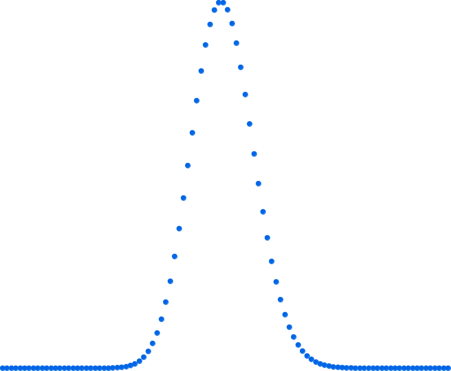
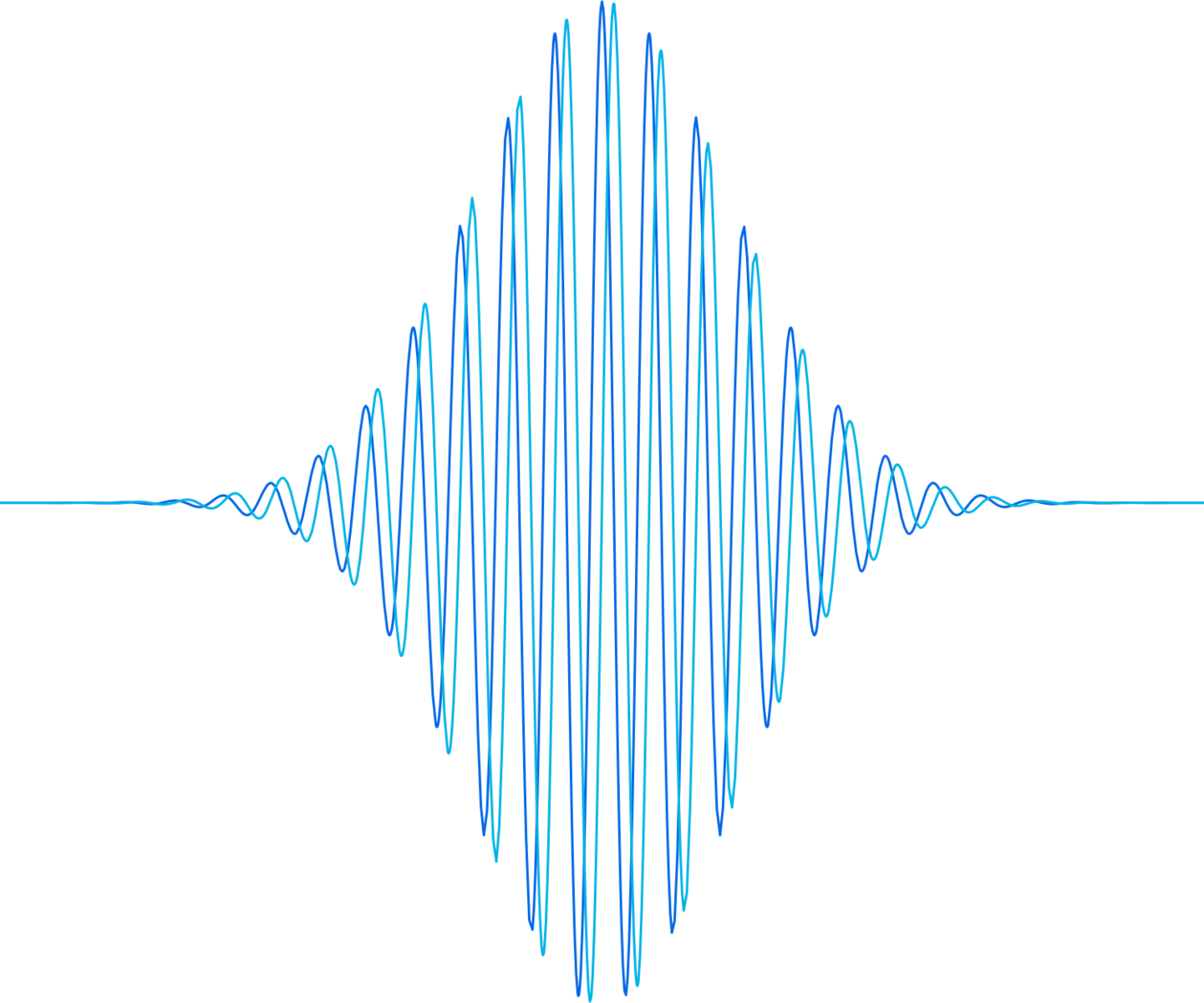
Figure 2: The Taylor coefficients of the function $e^{t(z-1)}$ and the plot of its real and imaginary part on the unit circle for large $t$. The former is the Poisson distribution with mean $t$ and standard deviation $\sqrt{t}$. The latter is localized on the $\frac{1}{\sqrt{t}}$ scale.

2.7.8

Let $\boldsymbol{f}_{t}$ be a sequence of functions such that

$$\boldsymbol{f}_{t}(e^{s/t})\to f(s)$$ (96)

on compact sets as $t\to\infty$. We define $\int_{\mathsf{X}}c$ by

$$\left\langle\int_{\mathsf{X}}e^{c_{1}(\mathscr{L})}c,f\right\rangle=\left[t^{\textup{vir}\dim\mathsf{X}/\mathsf{G}-\sum k_{i}}\right]\left\langle\chi(\mathsf{X},e^{(\mathscr{L}-1)t}\,\mathbf{c}),\boldsymbol{f}_{t}\right\rangle\,,$$ (97)

where bracket means we extract the corresponding term in the asymptotic expansion. It is easy to see this is independent of $\mathscr{L}$, see e.g.  Proposition 2.9 below.

Since $\boldsymbol{\psi}(\mathsf{X})$ is the generating function for the equivariant Chern classes of the tangent bundle, the equality (97) implies

$$\left\langle\int_{\mathsf{X}}e^{c_{1}(\mathscr{L})}\psi(T\mathsf{X}),f\right\rangle=\left[t^{\textup{vir}\dim\mathsf{X}/\mathsf{G}}\right]\left\langle\chi(\mathsf{X},e^{(\mathscr{L}-1)t}\boldsymbol{\psi}_{t}(T\mathsf{X})),\boldsymbol{f}_{t}\right\rangle\,,$$ (98)

where $\boldsymbol{\psi}_{t}(e^{s/t})\to\psi(s)$, and where we assume that $\psi(T\mathsf{X})$ grows at most polynomially in the imaginary direction.

2.7.9 Example $\mathsf{X}=\mathbb{P}^{1}$

Consider $\mathsf{X}=\mathbb{P}^{1}$ with the standard action of $\mathbb{C}^{\times}$. We denote by $x$ and $s$ elements of $\mathbb{C}^{\times}$ and $\operatorname{Lie}\mathbb{C}^{\times}$, respectively. Since $\mathbb{P}^{1}$ is smooth and proper, we have

$$\boldsymbol{\psi}(\mathbb{P}^{1})=\frac{\boldsymbol{\psi}(x)}{1-x^{-1}}+\frac{\boldsymbol{\psi}(x^{-1})}{1-x}\,,\quad\psi(\mathbb{P}^{1})=\frac{\psi(s)-\psi(-s)}{s}\,,$$ (99)

by localization. More generally, if $\mathscr{L}$ is a line bundle on $\mathbb{P}^{1}$ with $\mathbb{C}^{\times}$-weights $l_{0},l_{\infty}\in\mathbb{Z}$ at the two fixed points, then

$$\mathscr{L}^{k}\boldsymbol{\psi}(\mathbb{P}^{1}) =x^{kl_{0}}\frac{\boldsymbol{\psi}(x)}{1-x^{-1}}+x^{kl_{\infty}}\frac{\boldsymbol{\psi}(x^{-1})}{1-x}\,,$$

$$e^{c_{1}(\mathscr{L})}\psi(\mathbb{P}^{1}) =\frac{e^{l_{0}s}\psi(s)-e^{-l_{\infty}s}\psi(-s)}{s}\,.$$ (100)

Let us see how the formula (100) appears from the limit (98).

Ampleness of $\mathscr{L}$ is equivalent to $l_{0}>l_{\infty}$. Then, by the geometric series expansion, we have

$$\widehat{\chi(\mathscr{L}^{k}(T\mathbb{P}^{1})^{\otimes n})}=\delta_{[kl_{\infty}-n,kl_{0}+n]}\,,$$

viewed as function on $\mathbb{Z}$. Thus in the $k\to\infty$ limit, we have

$$\widehat{e^{c_{1}(\mathscr{L})}} =\delta_{[l_{\infty},l_{0}]} =\lim_{k\to\infty}k^{-1}\widehat{\chi(\mathscr{L}^{k})}\Big{|}_{\textup{scale the argument by $k^{-1}$}}\,,$$ (101)

$$\widehat{c_{1}(T\mathbb{P}^{1})} =\frac{\partial}{\partial l_{0}}-\frac{\partial}{\partial l_{\infty}} =\lim_{k\to\infty}k(\widehat{T\mathbb{P}^{1}}-1)\,,$$ (102)

where we interpret (102) as an operator acting on (101). Upon Fourier transform, this becomes (100).

2.7.10 Example $\mathsf{X}=\mathbb{C}^{1}$ and $\mathsf{X}=\operatorname{Thom}(0\to\mathbb{C}^{1})$

Note that if we take $\mathsf{X}=\mathbb{C}^{1}=\mathbb{P}^{1}\setminus\infty$, the same reasoning as in the previous example will yield the distribution

$$\widehat{e^{c_{1}(\mathscr{L})_{\mathbb{C}^{1}}}}=\delta_{[-\infty,l_{0}]}\Rightarrow e^{c_{1}(\mathscr{L})_{\mathbb{C}^{1}}}=\frac{e^{l_{0}s}}{s+0}\,,$$

where the shift of the pole indicate the direction of the deformation of the integration contour. In this case, the contour goes to the region $\Re s>0$, which is the infinitesimal analog of the shift in Example 2.2.4.

For $\mathsf{X}=\operatorname{Thom}(0\to\mathbb{C}^{1})$, we get

$$\widehat{\chi(\operatorname{Thom},\mathscr{L}^{k})}=-\delta_{[kl_{0}+1,\infty]}\,,$$

and thus

$$\widehat{e^{c_{1}(\mathscr{L})_{\operatorname{Thom}}}}=-\delta_{[l_{0},\infty]}\Rightarrow e^{c_{1}(\mathscr{L})_{\operatorname{Thom}}}=\frac{e^{l_{0}s}}{s-0}\,.$$

Since

$$\mathbb{P}^{1}=\mathbb{C}^{1}+\operatorname{Thom}(\infty\to\mathbb{P}^{1})$$

and $s$ acts on $T_{\infty}\mathbb{P}^{1}$ with weight $-1$, this agrees with the previous computation.

2.7.11

In this paper, we frequently use integral formulas that express $\boldsymbol{\psi}(\mathsf{X})$ as integrals over certain cycles $\gamma\subset\mathsf{A}$ in the maximal torus of $\mathsf{G}$ with density built from the functions $\boldsymbol{\psi}(x)$ and $(1-x^{-1})$. From such formulas, one can easily derive an integral formula for $\psi(\mathsf{X})$ by making the change of variables prescribed in the definition (98) and letting $t\to\infty$.

Note that in this limit, one should send all Lie groups elements to the identity at comparable rates. Since we use $q\in\mathbb{C}^{\times}$ as an important parameter in this paper, we may parametrize the limit in (98) by

$$t=\left(\ln q\right)^{-1}\,,\quad q\downarrow 1\,.$$

This means we replace the exponential map by the map $\xi\mapsto q^{\xi}$.

2.7.12

Proposition 2.9.

Integral formulas for the K-theoretic genus $\boldsymbol{\psi}(\mathsf{X})$ and the cohomological genus $\psi(\mathsf{X})$ are related by the correspondence in Table 1.

	$\operatorname{char}\mathbb{F}>0$	$\operatorname{char}\mathbb{F}=0$
cohomology theory	K-theory	cohomology
$\mathscr{Q}_{q}^{\vee}\cong$	$(\mathbb{C}^{\times},\,\cdot\,,1)$	$(\mathbb{C},+,0)$
Haar measure	$(2\pi ix)^{-1}dx$	$(2\pi i)^{-1}ds$
$\Psi=$	$\boldsymbol{\psi}(x)/(1-x^{-1})$	$\psi(s)/s$
$Z=$	$\Psi(1/x)\Psi(x/q)$	$\Psi(-s)\Psi(s-1)$
poles of $Z$	$x=1,q$	$s=0,1$
integration cycle	$\gamma\subset\mathsf{A}$	$\log_{q}(\gamma)_{0}\subset\mathfrak{a}$

Table 1: Conversion of formulas between the cases of finite and zero characteristic. The Haar measure $(2\pi i)^{-1}ds$ on Lie algebras of compact tori is normalized so that $\operatorname{Ker}\exp$ is a unimodular lattice. The subscript $\log_{q}(\gamma)_{0}$ means the component that does not escape to infinity as $q\to 1$. The cohomology column is the limit of the K-theory column in the sense explained in this Section.

Proof.

Substitute $g=q^{\xi}$ in the integral formula for $\langle\boldsymbol{\psi}(\mathsf{X}),e^{(\mathscr{L}-1)t}\,\boldsymbol{f}\rangle$. By definition, this transforms $\boldsymbol{\psi}(x)$ and $\boldsymbol{f}(g)$ into the corresponding $\psi(s)$ and $f(\xi)$, while affecting the other terms in the formula by

$$\frac{dx}{2\pi ix}\mapsto\ln q\,\frac{ds}{2\pi i}\,,\qquad\Psi(x)\mapsto\frac{1}{\ln q}\frac{\psi(s)}{s}\,.$$ (103)

The difference between the numbers of terms each kind is precise minus the virtual dimension of $\mathsf{X}/\mathsf{G}$, thus we get the correct power of $t$ as a prefactor.

The line bundle $\mathscr{L}$, being a function on the spectrum of K-theory, is represented by a regular function of the form

$$\mathscr{L}\big{|}_{q^{\xi}}=1+(\ln q)c_{1}(\mathscr{L})\big{|}_{\xi}+\dots$$

in the integral formulas. Therefore, $e^{(\mathscr{L}-1)t}\to e^{c_{1}(\mathscr{L})}$ as $q\to 1$.

The integration cycles $\gamma$ appearing in K-theoretic formulas have the form

$$\gamma=q^{\eta}\,\mathsf{H}_{\textup{cmp}}\big{/}\textup{conjugation}\,,$$

where $\mathsf{H}\subset\mathsf{G}$ is a reductive group, not necessarily connected, which commutes with $\eta$. Since

$$\textup{dist}_{\mathsf{G}}(1,\mathsf{H}_{\textup{cmp}}\setminus\mathsf{H}_{\textup{cmp},0})>\operatorname{const}>0\,,$$

the only component of $\log_{q}(\gamma)$ that does not escape to infinity as $q\to 1$ is

$$\log_{q}(\gamma)_{0}=\left(\eta+\mathfrak{h}_{\textup{cmp}}\right)\big{/}\textup{conjugation}\,.$$

This concludes the proof. ∎

As a corollary of the proof, we note that in cohomology we always integrate over a translate of a Lie algebra of a subtorus in $\mathsf{A}_{\textup{cmp}}$.

3 The stack $\mathscr{T}$

3.1 Basic properties

3.1.1

A central role in this paper will be played by the following derived quotient stack

$$\mathscr{T} =T^{*}(\mathsf{B}\backslash\mathsf{G}/\mathsf{B})$$ (104)

$$=T^{*}\mathscr{B}/\!\!/\!\!/\!\!/\mathsf{B}$$ (105)

$$=\{(e,\mathfrak{n}^{\prime}),e\in\mathfrak{n}\cap\mathfrak{n}^{\prime}\}/\mathsf{B}$$ (106)

$$=\{(e,\mathfrak{n}^{\prime},\mathfrak{n}^{\prime\prime}),e\in\mathfrak{n}^{\prime}\cap\mathfrak{n}^{\prime\prime}\}/\mathsf{G}$$ (107)

$$=\left(T^{*}\mathscr{B}\times_{\mathfrak{g}}T^{*}\mathscr{B}\right)/\mathsf{G}\,.$$ (108)

Here $/\!\!/\!\!/\!\!/\mathsf{B}$ in (105) denotes the algebraic symplectic reduction, that is, $\mu_{\mathfrak{b}}^{-1}(0)/B$, where $\mu_{\mathfrak{b}}^{-1}(0)$ is the derived preimage of $0\in\mathfrak{b}^{*}$ under the moment map. We denote by $\mathfrak{n}$ the nilradical of $\mathfrak{b}=\operatorname{Lie}\mathsf{B}$ and by $\mathfrak{n}^{\prime},\mathfrak{n}^{\prime\prime}\in\mathscr{B}$, viewed as parametrizing maximal nilpotent subalgebras of $\mathfrak{g}$, see Appendix A.3.

The equality between (104) and (105) is the definition of the cotangent bundle to a quotient stack. The equivalence of (105) and (106) follows from the identification of the Springer resolution

(109)

with the algebraic moment map $\mu$ for $\mathsf{G}$. Here, and in (193), we use the identification $\mathfrak{g}\cong\mathfrak{g}^{*}$ provided by an invariant bilinear form.

We call the stack $\mathscr{T}$ the Springer stack.

3.1.2

Via the presentation (104), we view $\psi(\mathscr{T})$ as a distribution on $\mathsf{A}\times\mathsf{A}$. We will compute it $\mathbb{C}^{\times}_{q}$-equivariantly, where $\mathbb{C}^{\times}_{q}$ scales the cotangent direction with weight $q^{-1}$.

3.1.3

From (107) we conclude that

$$\mathscr{T}=\bigcup_{e/\textup{conj}}\left(\mathscr{B}^{e}\times\mathscr{B}^{e}\right)/\mathsf{C}_{e}$$ (110)

where the union is over conjugacy classes of nilpotent elements of $\mathfrak{g}$, $\mathscr{B}^{e}$ is is the Springer fiber (196) of $e$, and $\mathsf{C}_{e}=\mathsf{G}^{e}$ is the centralizer of $e$. Compare with the formula (112) below.

Lemma 3.1.

We have the following equivalent expressions for the tangent bundle of $\mathscr{T}$

$$T\mathscr{T}\big{|}_{(e,\mathfrak{n},\mathfrak{n}^{\prime})} =\underbrace{(1+q^{-1})\mathfrak{g}}_{T_{(T^{*}\mathsf{G})}}-\underbrace{(\mathfrak{b}+q^{-1}\mathfrak{b}^{*})}_{/\!\!/\!\!/\!\!/\mathsf{B}}-\underbrace{(\mathfrak{b}^{\prime}+q^{-1}{\mathfrak{b}^{\prime}}^{*})}_{/\!\!/\!\!/\!\!/\mathsf{B}^{\prime}}$$ (111)

$$=\underbrace{(\mathfrak{n}^{*}-q^{-1}\mathfrak{n}^{*})}_{T_{\mathfrak{n}}\mathscr{B}^{e}}+\underbrace{({\mathfrak{n}^{\prime}}^{*}-q^{-1}{\mathfrak{n}^{\prime}}^{*})}_{T_{\mathfrak{n}^{\prime}}\mathscr{B}^{e}}+\underbrace{(q^{-1}\mathfrak{g}-\mathfrak{g})}_{T_{e}(\mathfrak{g}/\mathsf{G})}-2q^{-1}\mathfrak{a}$$ (112)

$$=\underbrace{q^{-1}\mathfrak{n}-\mathfrak{b}}_{T(\mathfrak{n}/\mathsf{B})}+\underbrace{\left(\mathfrak{n}^{\prime}\right)^{*}-q^{-1}\left(\mathfrak{b}^{\prime}\right)^{*}}_{\textup{$\mu$-relative tangent}}\,.$$ (113)

Here $\mathfrak{a}=\operatorname{Lie}\mathsf{A}$ and the virtual tangent bundle

$$T_{\mathfrak{n}}\mathscr{B}^{e}=\mathfrak{n}^{*}-q^{-1}\mathfrak{n}^{*}$$ (114)

describes $\mathscr{B}^{e}$ as the zero locus of the vector field $e$, see Appendix A.3.4.

Proof.

Formula (111) follows directly from (104), while the other two formulas are just restatements of (111). ∎

3.1.4

Via the presentation (108), we can view $\psi(\mathscr{T})$ as a distribution on

$$\mathsf{A}\times\mathsf{A}\times\mathbb{C}^{\times}_{q}\times\mathsf{G}\,.$$

The stabilizers of the nilpotent elements $e$ in the last two factors have the form

$$\widehat{\mathsf{C}}_{e}=\{(q,q^{h/2}\mathsf{C}_{e})\}\subset\mathbb{C}^{\times}_{q}\times\mathsf{G}\,,$$ (115)

$h$ being the characteristic of $e$, and the various $\widehat{\mathsf{C}}_{e}$ will correspond to the pieces of the eventual spectral decomposition. The integration over one of the $T^{*}\mathscr{B}$ factors in (110) will give the corresponding spectral projectors.

3.2 Characteristic classes of $\mathscr{T}$

3.2.1

First, we recall the computations of the $\mathsf{B}$-equivariant characteristic classes of

$$M=T^{*}\mathscr{B}\,.$$

This is the same as $\mathsf{A}$-equivariant characteristic classes for a maximal torus $\mathsf{A}\subset\mathsf{B}$.

3.2.2

We proceed by localization. The $\mathsf{A}$-fixed points on $M^{\mathsf{A}}$ are isolated and indexed by the Weyl group $W$. We will index the fixed points so that the smallest Bruhat cell corresponds to the longest element of the Weyl group. This means we take

$$M=T^{*}(\mathsf{G}/\mathsf{B}_{-})\,,$$ (116)

where $\mathsf{B}_{-}$ and $\mathsf{B}_{+}=\mathsf{B}$ is a pair of opposite Borel subgroups, and set

$$p_{w}=w\mathsf{B}_{-}\in\mathsf{G}/\mathsf{B}_{-}\subset M\,.$$

3.2.3

The positive roots of $\mathsf{G}$ will be, by definition, those contained in $\mathsf{B}_{+}$.

$$T_{p_{w}}M=w\cdot T_{p_{1}}M=w\left(\sum_{\alpha>0}(\alpha+q^{-1}/\alpha)\right)\,.$$

3.2.4

Recall that we view $\psi(\mathscr{T})$ as a distribution on $\mathsf{A}\times\mathsf{A}$, where the two copies act by the left and right regular action on $\mathsf{G}$. The point $w\in\mathsf{G}$ is fixed by a subtorus

$$\mathsf{A}\cong\textup{stabilizer}(w)=\{(a,w^{-1}\cdot a)\}\subset\mathsf{A}\times\mathsf{A}\,.$$

Thus, pairing the distribution with a test function

$$f_{1}\otimes f_{2}\in K_{\mathsf{A}\times\mathsf{A}}(\operatorname{pt})$$

means integrating $f_{1}(a)f_{2}(w^{-1}a)$ over $\mathsf{A}$.

Put it differently, the identification $f_{2}\in K_{\mathsf{A}}(\operatorname{pt})=K_{\mathsf{B}}(\operatorname{pt})=K_{\mathsf{G}}(\mathsf{G}/\mathsf{B})$ takes a $\mathsf{B}$-module $V$ to a vector bundle $\mathscr{V}=\mathsf{G}\times_{\mathsf{B}}V$ over $\mathsf{G}/\mathsf{B}$. The torus $\mathsf{A}$ acts on its fiber

$$\mathscr{V}_{p_{w}}=w\mathsf{B}\times_{\mathsf{B}}V\cong V$$

by the action of $w^{-1}\cdot a$ on $V$, whence the term $f_{2}(w^{-1}a)$ above. Here the choice of the Borel subgroup containing $\mathsf{A}$ is not material, which is why we have dropped the subscript in $\mathsf{B}_{-}$.

3.2.5

The tangent bundle to $\mathscr{T}$ has the following description:

$$T\mathscr{T} =T\left(M/\!\!/\!\!/\!\!/\mathsf{B}_{+}\right)$$

$$=TM-\mathfrak{b}_{+}-q^{-1}\mathfrak{b}_{-}\,.$$ (117)

Therefore,

$$T_{p_{w}}(T^{*}(\mathsf{B}_{+}\backslash\mathsf{G}/\mathsf{B}_{-})) =\sum_{\begin{subarray}{c}\alpha>0\\ w^{-1}\alpha<0\end{subarray}}(\alpha^{-1}-\alpha)(1-q^{-1})-(1+q^{-1})\mathfrak{a}\,.$$ (118)

and hence

$$\psi(\mathscr{T})\big{|}_{p_{w}}=\frac{1}{\textup{\small\cursive z}^{r}}\prod_{\begin{subarray}{c}\alpha>0\\ w^{-1}\alpha<0\end{subarray}}\frac{Z(x^{\alpha})}{Z(qx^{\alpha})}\,.$$

Where the function

$$Z(x)=\Psi(x^{-1})\Psi(x/q)$$ (119)

was introduced in (26). Here and in what follows we drop the subscript in $Z_{\psi}$ for brevity. We also define

$$\textup{\small\cursive z}=\psi(1)\Psi(q^{-1})\,.$$ (120)

3.2.6

Theorem 6.

Let $f_{1}\otimes f_{2}$ be a function on $\mathsf{A}\times\mathsf{A}$. We have

$$\left(f_{1}\otimes f_{2},\psi(\mathscr{T})\right)=\frac{1}{\textup{\small\cursive z}^{r}}\int_{\varsigma A_{\textup{cmp}}}d_{\textup{Haar}}\,\sum_{w}f_{1}(x)\,f_{2}(w^{-1}x)\prod_{\begin{subarray}{c}\alpha>0\\ w^{-1}\alpha<0\end{subarray}}\frac{Z(x^{\alpha})}{Z(qx^{\alpha})}\,,$$ (121)

for any $\varsigma\in\mathsf{A}$ such that

$$\forall\alpha>0\,,\quad|\varsigma^{\alpha}|>|q|\,.$$

Proof.

Since the vertical maps in the diagram

(122)

are proper, we can push forward the computation to $\mathfrak{n}/\mathsf{B}$.

Now, $\mathfrak{n}$ is a linear space, $\mathfrak{n}^{\mathsf{B}}=\{0\}$, and the normal $\mathsf{T}$-weights at $0$ have the form $\{q^{-1}x^{\alpha}\}$, where $\alpha>0$. With our assumption, all of these weights are attractive on $\varsigma A_{\textup{cmp}}$, whence the conclusion. ∎

To shorten the notation, one is tempted to replace $w$ by $w^{-1}$ in (121). We leave it as is because in this way we have the action of $w$ on parts of the integrand.

Corollary 3.2.

Theorem 3 holds for a certain normalization of measures.

We discuss the precise normalization of measures in Appendix A.4.

3.3 Stratification of $\mathscr{T}$

3.3.1

We now consider the stratification of $\mathscr{T}$ from (110). On each piece, we will consider the action of the stabilizer $\widehat{\mathsf{C}}_{e}$ from (115). We begin with

$$\operatorname{Slice}_{e}\mathfrak{g}=e+\mathfrak{g}^{e_{-}}\,,$$ (123)

where

$$e_{-}=\phi\left(\begin{bmatrix}0&0\\ 1&0\end{bmatrix}\right)\,.$$

Concerning the action of $(q,q^{h/2})\in\widehat{\mathsf{C}}_{e}$, we have the following

Lemma 3.3.

The weights of the $(q,q^{h/2})$-action on the slice (123) are repelling.

Proof.

The $h$-weights of $\mathfrak{g}^{e_{-}}$ are nonpositive by the representation theory of $\mathfrak{sl}_{2}$, and we have the additional factor of $q^{-1}$ coming from the scaling action of $\mathbb{C}^{\times}_{q}$. ∎

3.3.2

We now consider the $\widehat{\mathsf{C}}_{e}$-action on the fibers of projection to $\mathfrak{g}$ and note that the $\mathbb{C}^{\times}_{q}$ acts trivially on these fibers. We have the following classical result of De Concini, Lusztig, and Procesi.

Theorem 7 ([dCLP]).

The fixed loci and the attracting manifolds of the $q^{h/2}$-action on $\mathscr{B}^{e}$ are smooth.

3.3.3 Proof of Theorem 4

Stratify both copies of $\mathscr{B}^{e}$ by attracting manifolds of the $q^{h/2}$-action. Each piece is smooth, and the normal weights to it are repelling in the base $\mathfrak{g}$ by Lemma 3.3 and in the fiber by construction. Since the fixed loci are proper, and hence cohomologically proper, we can apply the results of Sections 2.6.5 and 2.6.6 to this stratification, proving the claim. ∎

3.4 Explicit formulas

3.4.1

By its definition (31), the bordism class of $\mathscr{B}^{e}$ is independent of $e$ and well-defined $\mathsf{G}$-equivariantly. Its characteristic classes can be easily computed by equivariant localization. To set it up, we fix a Borel subgroup $\mathsf{B}\subset\mathsf{G}$ with a maximal torus $\mathsf{A}\subset\mathsf{B}$ and define

$$\mathscr{P}_{\mathsf{B}}f=\left(\sum_{w\in W}w\right)\,\boldsymbol{\Pi}_{\mathsf{B}}\,f\,,\quad\boldsymbol{\Pi}_{\mathsf{B}}=\prod_{\alpha\notin\operatorname{Lie}\mathsf{B}}\frac{\Psi(x^{\alpha})}{\Psi(q^{-1}x^{\alpha})}\,.$$ (124)

From definitions and (31), we obtain the following

Proposition 3.4.

We have

$$\chi(f\otimes\psi([\mathscr{B}^{e}]))=\mathscr{P}_{\mathsf{B}}f\in K_{\mathsf{G}}(\operatorname{pt})_{\textup{an}}\,,$$ (125)

where we use the identification $f\in K_{\mathsf{A}}(\operatorname{pt})=K_{\mathsf{G}}(\mathsf{G}/\mathsf{B})\cong K_{\mathsf{G}}(\mathscr{B})$  .

In particular, the operators $\mathscr{P}_{\pm}$ from (34) correspond to the two Borel subgroups $\mathsf{B}_{\pm}$ used in Section 3.2.

3.4.2

For a given nilpotent $e$ we will be interested in the restriction $\left(\mathscr{P}_{\pm}\right)|_{\widehat{\mathsf{C}}_{e}}$ where $\widehat{\mathsf{C}}_{e}$ is the stabilizer (115).

We recall from Appendix A.3.3 that $W^{h}\backslash W$ cosets parametrize connected components of $\mathscr{B}^{h}$. We define

$$W(e)=\left\{w\in W\,\big{|}\,\mathscr{B}^{e}\cap\{\textup{corresponding component of $\mathscr{B}^{h}$}\}\neq\varnothing\right\}\,.$$

This set varies from $W(0)=W$ to

$$|W(\textup{regular nilpotent})|=1\,.$$

Lemma 3.5.

$$\Big{(}\mathscr{P}_{\pm}\Big{)}\Big{|}_{\widehat{\mathsf{C}}_{e}}=\Big{(}\sum_{w\in W(e)}w\,\boldsymbol{\Pi}_{\mathsf{B}}\,f\Big{)}\Big{|}_{\widehat{\mathsf{C}}_{e}}\,.$$ (126)

Proof.

In the equivariant localization computation, the contribution of those components of $\mathscr{B}^{h}$ that do not meet $\mathscr{B}^{e}$ vanishes in $\widehat{\mathsf{C}}_{e}$-equivariant K-theory. ∎

3.4.3

Consider the Lie algebras $\mathfrak{c}_{e}=\operatorname{Lie}\mathsf{C}_{e}$ and its $h$-grading

$$\mathfrak{c}_{e}=\mathfrak{c}_{e,0}\oplus\mathfrak{c}_{e,>0}\,,\quad\mathfrak{c}_{e,0}=\mathfrak{c}_{\phi}=\operatorname{Lie}\mathsf{C}_{\phi}\,.$$

The $\mathfrak{c}_{e,>0}$ term above is the Lie algebra of the unipotent radical of $\mathsf{C}_{e}$. We define

$$\Psi_{e}=\frac{1}{\Psi(q^{-1})^{2r}}\frac{\Psi(\operatorname{Slice}_{e}q^{-1}\mathfrak{g})}{\psi(\mathfrak{c}_{\phi})\Psi(\mathfrak{c}_{e,>0})}\,.$$ (127)

Since

$$q^{-1}T\operatorname{Slice}_{e}\mathfrak{g}-\mathfrak{c}_{e}=(q^{-1}-1)\mathfrak{g}$$ (128)

the density $\Psi_{e}$ is always the restriction to $\widehat{\mathsf{C}}_{e}$ of a $\mathsf{G}$-invariant quantity.

Theorem 8.

We have

$$(f_{1}\otimes f_{2},\psi(\mathscr{T}))=\sum_{\begin{subarray}{c}{\textup{nilpotent elements $e\in\mathfrak{g}$ \quad}}\\ \textup{up to conjugation}\end{subarray}}\int_{q^{h/2}\mathsf{C}_{\phi,\textup{cmp}}}\left(\mathscr{P}_{+}f_{1}\right)\left(\mathscr{P}_{-}f_{2}\right)\Psi_{e}\,d_{\textup{Haar}}\,.$$ (129)

Proof.

We apply Theorem 4, and specifically equation (29). The result of pushforward along two copies of $\mathscr{B}^{e}$ is given by $\left(\mathscr{P}_{+}f_{1}\right)\left(\mathscr{P}_{-}f_{2}\right)$. The contribution of the slice is the numerator in (127). Finally, we compute the $\mathsf{C}_{e}$-cohomology as described in Section 2.3.4. ∎

3.4.4

Since (129) is an equality between distributions having compact support, by analytic continuation we conclude the following

Corollary 3.6.

The equality (129) holds for functions $\psi$ analytic and nonvanishing in the annulus $1/R_{\mathsf{G}}<|x|<R_{\mathsf{G}}$, where $R_{\mathsf{G}}$ is a sufficiently large number that depends on $\mathsf{G}$.

3.5 Example: zero nilpotent

3.5.1

In the case $(h,e)=(0,0)$ we have

$$\mathscr{B}^{e}=\mathscr{B}\,,\quad\mathsf{C}_{\phi}=\mathsf{G}\,,$$

and thus the integration is over

$$(\mathscr{B})^{\times 2}/\mathsf{G}\cong\mathsf{B}\backslash\mathsf{G}/\mathsf{B}\,.$$

By definition of $\mathscr{T}$, we have

$$T\mathscr{T}\big{|}_{(0,\mathfrak{n},\mathfrak{n}^{\prime})} =\underbrace{(\mathfrak{n}^{*}+\mathfrak{n}^{\prime*}-\mathfrak{g})}_{T(\mathsf{B}\backslash\mathsf{G}/\mathsf{B})}+q^{-1}\underbrace{(\mathfrak{n}+\mathfrak{n}^{\prime}-\mathfrak{g})}_{T^{*}(\mathsf{B}\backslash\mathsf{G}/\mathsf{B})}\,.$$ (130)

Therefore, the $e=0$ term in (129) is given by the same integral as in (121), except the cycle of the integration is the compact torus.

3.5.2

We now trace this equality through formulas. We have

$$\operatorname{Slice}_{0}\mathfrak{g}=\mathfrak{g},\quad\mathfrak{c}_{\phi}=\mathfrak{g}\,,$$

and therefore

$$\Psi_{e}=\frac{\Psi(q^{-1}\mathfrak{g})}{\psi(\mathfrak{g})}\,.$$

Echoing (128), we note that $\Psi_{e}$ is $W$-invariant. The Weyl integration formula gives

$$\int_{\mathsf{G}_{\textup{cmp}}}\left(\mathscr{P}_{+}f_{1}\right)\left(\mathscr{P}_{-}f_{2}\right)\Psi_{\phi}\,d_{\textup{Haar}}=$$

$$=\frac{1}{|W|}\frac{1}{\psi(1)^{r}\Psi(q^{-1})^{r}} \int_{\mathsf{A}_{\textup{cmp}}}\left(\mathscr{P}_{+}f_{1}\right)\left(\mathscr{P}_{-}f_{2}\right)\prod_{\alpha\neq 0}\frac{\Psi(q^{-1}x^{\alpha})}{\Psi(x^{\alpha})}\,d_{\textup{Haar}}$$

$$=\frac{1}{\psi(1)^{r}\Psi(q^{-1})^{r}} \int_{\mathsf{A}_{\textup{cmp}}}f_{1}\left(\mathscr{P}_{-}f_{2}\right)\prod_{\alpha>0}\frac{\Psi(q^{-1}x^{\alpha})}{\Psi(x^{\alpha})}\,d_{\textup{Haar}}$$

$$=\frac{1}{\psi(1)^{r}\Psi(q^{-1})^{r}} \int_{\mathsf{A}_{\textup{cmp}}}f_{1}\left(\mathscr{P}_{\textup{Langl}}\,f_{2}\right)d_{\textup{Haar}}\,,$$ (131)

where we used the $W$-invariance in going from the second line to the third, and (33) to pass from the third line to the fourth. Clearly, this is the integral (121) taken over the compact torus.

3.6 Example: regular nilpotent

3.6.1

In this case we have

$$h=2\rho^{\vee}\,,\quad\mathfrak{c}_{\phi}=0\,,\quad W^{h}=\{1\}\,,$$

and $\mathsf{C}_{\phi}$ is the center of $\mathsf{G}$

$$\mathsf{C}_{\phi}=\mathsf{C}(\mathsf{G})=\left\{x\in\mathsf{A}\,\big{|}\,\forall\alpha\,,x^{\alpha}=1\right\}\,.$$

3.6.2

We have

$$\alpha(h/2)=\operatorname{ht}(\alpha)\,,\quad\alpha>0\,,$$

where $\operatorname{ht}(\alpha)$ denotes the height of a positive root. For negative roots, we define height by the above equality. We see that

$$\Big{(}w\boldsymbol{\Pi}_{\pm}\Big{)}\Big{|}_{\widehat{\mathsf{C}}_{e}}=\begin{cases}\displaystyle{\prod_{\alpha<0}\dfrac{\Psi(q^{\operatorname{ht}(\alpha)})}{\Psi(q^{-1+\operatorname{ht}(\alpha)})}}\,,&\textup{$w=1$ for $\mathbb{P}_{+}$, $w=w_{0}$ for $\mathbb{P}_{-}$}\,,\textup{resp.}\,,\\ 0\,,&\textup{otherwise}\,,\end{cases}$$ (132)

where $w_{0}$ is the longest element. By Lemma 3.5, this reflects the fact that $\mathscr{B}^{e}$ is fat point and meets only one point in $\mathscr{B}^{h}$.

3.6.3

The classical identity, see e.g. [Kostant, Macdonald, Steinberg],

$$(1-q^{-1})\sum_{\alpha>0}q^{\operatorname{ht}(\alpha)}=\sum_{\textup{exponents $m_{i}$}}q^{m_{i}}-r$$ (133)

connecting the heights of the positive roots and the exponents of a Lie algebra $\mathfrak{g}$ implies that

$$\displaystyle{\prod_{\alpha<0}\dfrac{\Psi(q^{\operatorname{ht}(\alpha)})}{\Psi(q^{-1+\operatorname{ht}(\alpha)})}} =\Psi\left((1-q^{-1})\sum_{\alpha>0}q^{-\operatorname{ht}(\alpha)}\right)$$

$$=\Psi\left(-\sum_{\alpha>0}q^{-m_{i}-1}+rq^{-1}\right)$$ (134)

3.6.4

Similarly, we observe that $\Psi_{e}$ is the $\Psi(\dots)$ where dots stand for the following expression

$$(q^{-1}-1)\mathfrak{g}\Big{|}_{q^{h/2}}-2rq^{-1} =-(1+q^{-1})r+(q^{-1}-1)\sum_{\alpha\neq 0}q^{\operatorname{ht}(\alpha)}$$

$$=\sum\left(q^{-m_{i}-1}-q^{m_{i}}\right)-2rq^{-1}\,.$$ (135)

This means that

$$\left(\mathscr{P}_{+}f_{1}\right)\left(\mathscr{P}_{-}f_{2}\right)\Psi_{e}\Big{|}_{x\in q^{h/2}\mathsf{C}_{e}}=\frac{1}{\prod Z(q^{m_{i}+1})}f_{1}(x)f_{2}(w_{0}x)$$ (136)

and

$$\int_{q^{h/2}\mathsf{C}_{\phi,\textup{cmp}}}\textup{\eqref{eq:17} }\,d_{\textup{Haar}}=\frac{1}{|\mathsf{C}(\mathsf{G})|\prod Z(q^{m_{i}+1})}\sum_{x\in\mathsf{C}(\mathsf{G})}f_{1}(q^{\rho^{\vee}}x)f_{2}(q^{-\rho^{\vee}}x)\,,$$ (137)

where we have used the fact that $w_{0}$ takes $\rho^{\vee}$ to $-\rho^{\vee}$ and fixes the elements of $\mathsf{C}(\mathsf{G})$.

3.6.5

Formula (136) may be interpreted as picking up the residues in (121) at the $x^{\alpha}=q$ poles of the factor

$$\frac{1}{\psi(1)^{r}\Psi(q^{-1})^{r}}\prod_{\textup{simple $\alpha>0$}}Z(x^{\alpha})\prod\frac{dx_{j}}{2\pi ix_{j}}\,.$$ (138)

The simple roots $x^{\alpha}$ may be chosen as étale coordinates on $\mathsf{A}$ and the factor $|\mathsf{C}(\mathsf{G})|^{-1}$ appears as the Jacobian of this transformation. After that, each residue in (138) equals one since

$$Z(x)=\frac{\psi(1)\Psi(q^{-1})}{1-q/x}+O(|x-q|)\,.$$

4 Spectral Decomposition

4.1 Symmetric dependence on $\Psi$

4.1.1

Since the function $\Psi(x)$ appears in Theorem 6 only through the function $Z(x)$, it is worthwhile to recast Theorem 8 in a symmetric form.

To avoid creating matching pairs of zeros and poles, we introduce the entire invertible function

$$Z^{1}(x)=(1-1/x)(1-q/x)Z(x)=-x^{-1}\psi(1/x)\psi(x/q)\,.$$ (139)

Eventually, we will allow the function $Z$ to have zeros in the critical annulus, in which case $Z^{1}(x)$ will be an entire function with those zeros. In particular, in the geometric case, it will constitute the contribution of $H^{1}$ of the curve to the $\zeta$-function, whence the notation.

4.1.2

We define

$$\mathscr{P}^{Z}_{\pm}=\left(\prod_{\alpha\neq 0}\psi(q^{-1}x^{\alpha})\right)\mathscr{P}_{\pm}=\left(\sum_{w\in W}w\right)\,\prod_{\alpha\gtrless 0}\frac{1-qx^{\alpha}}{1-x^{-\alpha}}Z^{1}(x^{\alpha})\,.$$ (140)

and

$$Z_{e} =\frac{\Psi_{e}}{\prod_{\alpha\neq 0}\psi(q^{-1}x^{\alpha})^{2}}$$

$$=(-1)^{\dim\mathfrak{g}}(1-q)^{2r}\frac{\mathscr{O}_{\operatorname{Slice}_{e}q^{-1}\mathfrak{g}\big{/}\mathfrak{c}_{e,>0}}}{Z^{1}(\mathfrak{g})}\,,$$ (141)

where $\mathscr{O}$ in the numerator of (141) denotes the character of functions, that is, the product of $(1-w^{-1})^{-1}$ over all Chern roots $w$ of $\operatorname{Slice}_{e}q^{-1}\mathfrak{g}-\mathfrak{c}_{e,>0}$. In deriving (141) from (140) we used the fact that the adjoint representation $\mathfrak{g}$ is self-dual and has trivial determinant.

4.1.3

The density (141) can be conveniently expressed in terms of the multiplicity spaces $\mathfrak{g}_{i}^{e}$ in the decomposition

$$\mathfrak{g}=\sum_{i\geq 0}V^{i}\boxtimes\mathfrak{g}^{e}_{i}\,,$$ (142)

of $\mathfrak{g}$ as a $\phi(SL(2))\oplus\mathsf{C}_{\phi}$-module. Here $\mathfrak{g}_{i}$ are the $\operatorname{ad}(h)$-eigenspaces and $V^{i}$ is the irreducible $\mathfrak{sl}_{2}$-module with highest weight $i$. Recall that the existence of an invariant bilinear form on $\mathfrak{g}$ implies that $\mathfrak{g}_{i}^{*}\cong\mathfrak{g}_{-i}$ as $\mathsf{G}^{h}$-modules.

Lemma 4.1.

The $\mathsf{C}_{\phi}$-modules $\mathfrak{g}_{i}$ and $\mathfrak{g}_{i}^{e}$ are selfdual. The $\mathsf{C}_{\phi}$-module $\mathfrak{g}_{1}\cong\mathfrak{g}_{-1}$ is symplectic. We have

$$\det\bigoplus_{i\geq 0}\mathfrak{g}_{i}^{e}=1\,.$$

Proof.

From self-duality of $\mathfrak{g}$ and $V^{i}$ in (142), we conclude the self-duality of $\mathfrak{g}^{e}_{i}$. Since

$$\mathfrak{g}_{i}=\bigoplus_{j\in i+2\mathbb{Z}_{\geq_{0}}}\mathfrak{g}_{j}^{e}\,,$$ (143)

it follows these modules are similarly self-dual.

The module $\mathfrak{g}_{-1}$ has a skew-symmetric form

$$(\xi,\xi^{\prime})\mapsto([\xi,\xi^{\prime}],e)\,,$$

which is nondegenerate because $\operatorname{ad}(e)$ has no kernel in $\mathfrak{g}_{-1}$.

Finally, from (143) we conclude

$$\bigoplus_{i\geq 0}\mathfrak{g}_{i}^{e}=\mathfrak{g}_{0}\oplus\mathfrak{g}_{1}\,.$$

We have $\det\mathfrak{g}_{1}=1$ because $\mathfrak{g}_{1}$ is symplectic, and $\det\mathfrak{g}_{0}=1$ because $\mathfrak{g}_{0}$ is the Lie algebra of a reductive group $\mathsf{G}^{h}$. ∎

4.1.4

Theorem 8 can thus be restated as follows.

Proposition 4.2.

We have

$$(f_{1}\otimes f_{2},\psi(\mathscr{T}))=\sum_{e}\int_{q^{h/2}\mathsf{C}_{\phi,\textup{cmp}}}\left(\mathscr{P}^{Z}_{+}f_{1}\right)\left(\mathscr{P}_{-}^{Z}f_{2}\right)Z_{e}\,d_{\textup{Haar}}\,,$$ (144)

where $\mathscr{P}^{Z}_{\pm}$ is given by (140) and

$$Z_{e}\big{|}_{q^{h/2}c}=q^{-\frac{\dim\mathfrak{g}+\dim\mathfrak{g}^{e}}{2}}\frac{(1-q)^{2r}}{Z^{1}(\mathfrak{g})}\frac{\prod_{i>0}\det_{\mathfrak{g}_{i}^{e}}(1-q^{-i/2}c)\phantom{\,\,\,\,\,}}{\prod_{i\geq 0}\det_{\mathfrak{g}_{i}^{e}}(1-q^{-i/2-1}c)}\,,\quad c\in\mathsf{C}_{\phi}\,.$$ (145)

Proof.

We compute

$$(-1)^{\dim\mathfrak{g}}\operatorname{tr}_{\mathscr{O}_{\operatorname{Slice}_{e}q^{-1}\mathfrak{g}/\mathfrak{c}_{e,>0}}}q^{h/2}c =(-1)^{\dim\mathfrak{g}}\frac{\prod_{i>0}\det_{\mathfrak{g}_{i}^{e}}(1-q^{-i/2}c^{-1})\phantom{\,\,\,\,\,}}{\prod_{i\geq 0}\det_{\mathfrak{g}_{i}^{e}}(1-q^{+i/2+1}c^{-1})}$$

$$=q^{-\frac{\dim\mathfrak{g}+\dim\mathfrak{g}^{e}}{2}}\frac{\prod_{i>0}\det_{\mathfrak{g}_{i}^{e}}(1-q^{-i/2}c)\phantom{\,\,\,\,\,}}{\prod_{i\geq 0}\det_{\mathfrak{g}_{i}^{e}}(1-q^{-i/2-1}c)}\,,$$ (146)

where we have used the self-duality of $\mathfrak{g}_{i}^{e}$ in making the $c\mapsto c^{-1}$ change in the numerator, the triviality of the determinant of $c$ in $\bigoplus_{i\geq 0}\mathfrak{g}_{i}^{e}$, as we as the observations that

$$\dim\mathfrak{g}-\dim\mathfrak{g}^{e}=\dim\textup{Orbit}(e)\in 2\mathbb{Z}\,.$$

∎

4.2 Hermitian form

4.2.1

In equivariant K-theory there is a natural involution

$$\mathscr{V}^{*}=\operatorname{Hom}_{\mathbb{C}}(\mathscr{V},\mathbb{C})\,,$$

where $\mathbb{C}$ is the trivial bundle with the trivial action of all groups involved. We extend it to $K_{\mathsf{G}}(\mathsf{X})\otimes_{\mathbb{Z}}\mathbb{C}$ anti-linearly. Then, for instance, for

$$f\in K_{\mathsf{G}}(\operatorname{pt})\otimes\mathbb{C}\subset\mathbb{C}[\mathsf{G}]$$

we have

$$f^{*}(g)=\bar{f}(g^{-1})\,.$$

By definition, we set

$$\|f\|^{2}_{\Psi}=(f\boxtimes f^{*},\psi(\mathscr{T}))\,.$$ (147)

4.2.2

In this subsection, we will assume that

$$q >1\,,$$

$$Z(x) >0\,,\quad x>q\,,$$ (148)

$$Z^{1}(x) \neq 0\,,\quad x\in\mathbb{R}\setminus\{1<|x|<q\}\,.$$ (149)

By the functional equation, this implies that $Z(x)>0$ for $x\in(-1,1)\setminus\{0\}$. Recall that, so far, we assumed $\psi(x)$ to be nonvanishing. However, starting in Section 4.3, we will relax this condition to having no zeros in the critical annulus/strip. We reflect this weakening of assumptions in (149). Note that by the functional equation, (148) implies $Z(x)>0$ for $x\in(0,1)$. Also, (148) is equivalent to $Z^{1}(x)>0$ for $x\in\mathbb{R}_{>0}\setminus(1,q)$.

4.2.3

We have the following

Proposition 4.3.

With the assumptions (148) we have

$$\mathscr{P}_{-}^{Z}f^{*}\Big{|}_{q^{h/2}\mathsf{C}_{\phi,\textup{cmp}}}=\overline{\mathscr{P}_{+}^{Z}f}\Big{|}_{q^{h/2}\mathsf{C}_{\phi,\textup{cmp}}}$$

and $Z_{e}\geq 0$ on $q^{h/2}\mathsf{C}_{\phi,\textup{cmp}}$.

Proof.

Since the function $Z(x)$ is single-valued and real on a part of the real axis, it follows that it is real, that is, $\overline{Z(x)}=Z(\overline{x})$.

Consider an element of the form

$$x=q^{h/2}c\,,\quad c\in\mathsf{C}_{\phi,\textup{cmp}}\,,$$

and note that

$$\overline{x}=q^{h/2}\overline{c}\sim q^{h/2}c^{-1}\sim q^{-h/2}c^{-1}=x^{-1}\,,$$

where similarity means being conjugate in $\mathsf{G}$. Indeed, $\overline{c}\sim c^{-1}$ inside a maximal compact subgroup of $\mathsf{G}^{h}$, while $h$ is conjugate to $-h$ by the image of $\phi:SL(2)\to\mathsf{G}^{c}$. Since $\mathscr{P}_{+}^{Z}f$ is conjugation-invariant, we conclude

$$\overline{\mathscr{P}_{+}^{Z}f}\Big{|}_{x=q^{h/2}c}=\mathscr{P}_{+}^{Z}\overline{f}\Big{|}_{x^{-1}}=\mathscr{P}_{-}^{Z}f^{*}\Big{|}_{x}\,.$$

We now consider $Z_{e}$. Since eigenvalues of $c$ lie on the unit circle in complex conjugate pairs, we observe that all terms in (145) are positive, with the possible exception of $Z^{1}(\mathfrak{g})$.

The representations $\mathfrak{g}_{i}$ being self-dual, its $c$-weights appear either in complex conjugate pairs or are equal to $\pm 1$. We are thus left with the contributions of $Z^{1}(\pm q^{i/2})$.

By our assumption, $Z^{1}(q^{i/2})>0$, except possibly $Z^{1}(q^{1/2})$. However, the representation $\mathfrak{g}_{1}$ being symplectic by Lemma 4.1, the $q^{1/2}$-weights in $\mathfrak{g}_{1}$ appears with even multiplicity, hence its contribution is positive.

Now consider the contribution of $Z^{1}(-q^{i/2})$. By (149) all of these numbers are of the same sign, except possibly $Z^{1}(-q^{1/2})$, which appears with even multiplicity in the symplectic representation $\mathfrak{g}_{1}$. The nontrivial weights in the adjoint representation appear in pairs given by the opposite roots. In particular, the total number of negative real weights in $\mathfrak{g}$ is even for any element of $\mathsf{G}$. This completes the proof. ∎

As a corollary of the proof, we note the following

Corollary 4.4.

In the statement of Proposition 4.3, it suffices to assume that $Z(x)$ is real for $x>q$ and that $Z(x)^{\operatorname{rk}\mathsf{G}}>0$ for $x>q$.

Proof.

Indeed, the number of positive real eigenvalues in the adjoint representation has the same parity as $\operatorname{rk}\mathsf{G}$. ∎

4.2.4

Corollary 4.5.

With the assumptions (148) we have

$$\|f\|_{\Psi}^{2}=\sum_{e}\int_{q^{h/2}\mathsf{C}_{\phi,\textup{cmp}}}\left|\mathscr{P}_{+}f\right|^{2}\left|\Psi_{e}\right|\,d_{\textup{Haar}}\,.$$ (150)

Proof.

We have

$$Z_{e}=|Z_{e}|=\frac{|\Psi_{e}|}{\prod_{\alpha\neq 0}\psi(q^{-1}x^{\alpha})\overline{\psi(q^{-1}x^{\alpha})}}\,,$$

whence the conclusion. ∎

4.3 Zeros is the critical annulus

4.3.1

Our constructions so far assumed that the function $\psi(x)$ has no zeros or poles in the whole complex plane, with the extension by analytic continuations to functions holomorphic in a sufficiently large annulus as in Corollary 3.6.

Our next goal is to extend this result to functions having zeros in the annulus $q^{-1}<|x|<1$. For the function $Z(x)$ this means a pair of zeros in the critical annulus.

In the language of Sections 2.2.6 and 2.2.7, we check here that $\psi(T\mathscr{T})$ defines a regular function on $\operatorname{Spec}K(\mathscr{T})$, with pushforward given by the same formulas, even when $\psi$ does have zeros in the critical annulus.

4.3.2

If $M$ is smooth and proper, we have

$$\chi(M,\psi(TM)\otimes{\Omega}^{\raisebox{1.42262pt}{$\scriptscriptstyle\bullet$}}_{c}M)=\chi(M,\hat{\psi}(TM))$$

where

$${\Omega}^{\raisebox{1.42262pt}{$\scriptscriptstyle\bullet$}}_{c}M=\sum_{i}\Lambda^{i}\left(c\otimes T^{*}M\right)[-i]$$

and

$$\hat{\psi}(x)=(1-c/x)\,\psi(x)\,.$$

Note this creates a zero in the function $\hat{\psi}$ at $x=c$. We can interpret the parameter $c$ as equivariant variable for an extra copy of $\mathbb{C}^{\times}$ that acts trivially on $M$ but nontrivially on the bundle $T^{*}M$ whose characteristic class is inserted in the integral.

4.3.3

While our stack $\mathscr{T}$ is not a smooth manifold, we can consider the sequence

$$\Omega^{1}\mathscr{T}[-1]=\Big{(}q\mathfrak{b}\xrightarrow{\quad d\mu^{*}\quad}T^{*}M[-1]\xrightarrow{\quad\textup{action}^{*}\quad}\mathfrak{b}^{*}[-2]\Big{)}\,,$$ (151)

where $M=T^{*}\mathscr{B}$. This sequence is exact on $\mu^{-1}(0)$, or modulo the ideal generated by the coordinates of the moment map. We define

$${\Omega}^{\raisebox{1.42262pt}{$\scriptscriptstyle\bullet$}}_{c}\mathscr{T}=\textup{\v{C}ech}_{\mathfrak{m}}\left({\mathsf{S}}^{\raisebox{1.42262pt}{$\scriptscriptstyle\bullet$}}\left(c\otimes\Omega^{1}\mathscr{T}[-1]\right)\right)$$ (152)

where $\mathfrak{m}\subset{\mathsf{S}}^{\raisebox{1.42262pt}{$\scriptscriptstyle\bullet$}}\mathfrak{b}$ is the maximal ideal of the origin $0\in\mathfrak{b}^{*}$ and we take the Cech cohomology complex for the local cohomology at this point.

4.3.4

Given $a\in\mathsf{A}$, we define

$$\mathfrak{b}=\mathfrak{b}_{<}\oplus\mathfrak{b}_{\geq}$$

where $\mathfrak{b}_{<}$ is spanned by eigenvectors of $\operatorname{ad}(a)$ that are less then $1$ in absolute value.

Lemma 4.6.

Suppose that

$$|q|^{-1}<|c|<1$$

and that $\mathfrak{b}_{<}$ intersects trivially the stabilizer of $x\in M^{(q,a)}$. Then all but finitely many weights of the $(a,c,q)$-action on cohomology of the complex ${\Omega}^{\raisebox{1.42262pt}{$\scriptscriptstyle\bullet$}}_{c}\mathscr{T}\big{|}_{x}$ are less than $1$ in absolute value and

$$\chi\left({\Omega}^{\raisebox{1.42262pt}{$\scriptscriptstyle\bullet$}}_{c}\mathscr{T}\big{|}_{x}\right)=\textup{geometric series expansion of}\left(\frac{{\Omega}^{\raisebox{1.42262pt}{$\scriptscriptstyle\bullet$}}_{c}M}{{\Omega}^{\raisebox{1.42262pt}{$\scriptscriptstyle\bullet$}}_{c}\left(\mathfrak{b}\oplus q^{-1}\mathfrak{b}^{*}\right)}\right)\,.$$ (153)

Here we take the expansion that converges at the given element $(a,c,q)$.

Proof.

If $\mathfrak{b}_{<}$ injects into $T_{x}M$ then, dually, $T_{x}M$ surjects onto $\mathfrak{b}_{<}^{*}$. Thus we can write

$$\Omega^{1}\mathscr{T}[-1]=\Big{(}q\mathfrak{b}_{\geq}\xrightarrow{\quad}(T^{*}M)_{\geq}[-1]\xrightarrow{\quad}\mathfrak{b}^{*}_{\geq}[-2]\Big{)}$$

where

$$(T^{*}M)_{\geq}=\operatorname{Ker}(T^{*}M\to\mathfrak{b}^{*}_{<})/\mathfrak{b}_{<}\,,$$

is a locally free sheaf.

There is a spectral sequence from

$${\mathsf{S}}^{\raisebox{1.42262pt}{$\scriptscriptstyle\bullet$}}(c\otimes\mathfrak{b}_{\geq 0}^{*}[-2])\otimes{H}^{\raisebox{1.42262pt}{$\scriptscriptstyle\bullet$}}_{\mathfrak{m}}{\mathsf{S}}^{\raisebox{1.42262pt}{$\scriptscriptstyle\bullet$}}(qc\otimes\mathfrak{b}_{\geq 0})\otimes{\mathsf{S}}^{\raisebox{1.42262pt}{$\scriptscriptstyle\bullet$}}(c\otimes(T^{*}M)_{\geq}[-1])$$ (154)

to the cohomology of ${\Omega}^{\raisebox{1.42262pt}{$\scriptscriptstyle\bullet$}}_{c}\mathscr{T}$.

Under our assumption, the absolute values of the $(a,c,q)$-weights in $c\otimes\mathfrak{b}_{\geq}^{*}$ are strictly less than $1$, while the absolute values of the weight in $qc\otimes\mathfrak{b}_{\geq}$ are strictly bigger than $1$. This implies that the weights in the first two factors in (154) are less than $1$ and the corresponding Euler characteristics converge to a rational function. Since the third factor in (154) is finite-dimensional, it affect only finitely many weights and does not affect the convergence.

Since the Euler characteristic of (154) converges, we can forget about the differentials in the spectral sequence. This gives (153). ∎

4.3.5

Proposition 4.7.

The conditions of Lemma 4.6 are satisfied if $|a^{\alpha}|>1$ for all roots in $\mathfrak{b}$ or if $x$ lies over the point $e\in\mathfrak{n}$ and $a\in q^{h/2}\mathsf{C}_{\phi,\textup{cmp}}$.

Proof.

If

$$|a^{\alpha}|>1$$

for all roots then $\mathfrak{b}_{<}=0$ and there is nothing to check.

Since the stabilizer of $e$ in $\mathfrak{g}$ is contained in $\mathfrak{p}(h)$, we conclude that it intersects $\mathfrak{b}_{<0}$ trivially. Therefore, the stabilizer of $x$ intersects $\mathfrak{b}_{<0}$ trivially and the result follows. ∎

4.3.6

Corollary 4.8.

The equality (150) holds for functions $\psi$ analytic in the annulus $1/R_{\mathsf{G}}<|x|<R_{\mathsf{G}}$ and nonvanishing outside of the critical strip $|q|^{-1}<x<1$, where $R_{\mathsf{G}}$ is a sufficiently large number that depends on $\mathsf{G}$.

Proof.

We make the substitution

$$\hat{\psi}(\mathscr{T})=\psi(\mathscr{T})\otimes\bigotimes{\Omega}^{\raisebox{1.42262pt}{$\scriptscriptstyle\bullet$}}_{c_{i}}\mathscr{T}$$

where all $c_{i}$ lie in the critical strip. The new genus $\psi(x)$ has zeroes $c_{i}$ in the critical strip.

By Proposition 4.7 the insertion of ${\Omega}^{\raisebox{1.42262pt}{$\scriptscriptstyle\bullet$}}_{c_{i}}\mathscr{T}$ does not affect cohomological properness in either Theorem 6 or in the integration over strata in Theorem 4, whence the conclusion. ∎

4.4 Proof of Theorems 5 and 2

4.4.1 Proof of Theorem 5

We first consider the K-theory case. The difference between the statement of Corollary 4.8 and (37) is the domain of the integration, namely $\widetilde{\mathbf{S}}_{e}$ versus $\mathbf{S}_{e}$. We recall that $\mathscr{P}_{+}f$ is the restriction to $\widetilde{\mathbf{S}}_{e}$ of a conjugation-invariant function on $\mathsf{G}$. Similarly, as observed in Section 3.4.3, the density $\Psi_{e}$ is a restriction of a conjugation-invariant functions. Thus the integrand in (150) is pulled back from $\mathbf{S}_{e}$, while the Haar measure on $\mathbf{S}_{e}$ is pushed forward from $\widetilde{\mathbf{S}}_{e}$, the equality (37) in the K-theory case.

4.4.2

The cohomology case follows from the K-theory by taking a limit as explained in Section 2.7. While this concludes the proof, it may be instructive to see explicit formulas below.

4.4.3

Since, in this paper, we focus on the more difficult K-theoretic computations, it may be useful to spell out the formulas one obtains in the specialization to cohomology.

The combination of Theorems 6 and 5 may be phrased as the following equality of integrals involving general functions $\psi(s)$ and $f(s)$, analytic in a sufficiently wide neighborhood of the imaginary axis. We define

$$\Psi(s)=\frac{\psi(s)}{s}\,,\quad Z_{\psi}(s)=\Psi(-s)\Psi(s-1)$$

and denote

$$\textup{\small\cursive z}_{\psi}=-\psi(0)\psi(-1)\,.$$

We require that:

1. $\psi(s)$ is nonvanishing outside the vertical strip $-1<\Re s<0$ ,

2. $Z_{\psi}(s)$ is real and positive for $s>1$ ,

3. The integrals on both sides of (155) converge. For example, this can be guaranteed by $f$ being a Paley-Wiener function and $\psi(s\pm 1)/\psi(s)$ growing at most polynomially in the imaginary direction.

In this setting, the combination of Theorems 6 and 5 implies the following equality:

$$\frac{1}{\textup{\small\cursive z}_{\psi}^{r}}\int_{\Re x=x_{0}>\rho^{\vee}}\,\sum_{w}f(x)\,\overline{f}(-w^{-1}x)\prod_{\begin{subarray}{c}\alpha>0\\ w^{-1}\alpha<0\end{subarray}}\frac{Z_{\psi}(\alpha(x))}{Z_{\psi}(1+\alpha(x))}\,dx=\\ \\ =\sum_{\phi}\int_{\frac{1}{2}\phi(h)+\operatorname{Lie}\mathsf{C}_{\phi,\textup{cmp}}}\left|\mathscr{P}_{+}f\right|^{2}\,|\Psi_{e}|\,dx\,.$$ (155)

Here the summation is over the homomorphisms

$$\phi:\mathfrak{sl}_{2}\to\mathfrak{g}\,,$$

considered up to conjugation, and uses the image of the standard basis

$$h=\begin{pmatrix}1&0\\ 0&-1\end{pmatrix}\,,\quad e=\begin{pmatrix}0&1\\ 0&0\end{pmatrix}\quad e_{-}=\begin{pmatrix}0&0\\ 1&0\end{pmatrix}\,,$$

in $\mathfrak{g}$. The the integration is over a shift by $\tfrac{1}{2}\phi(h)$ of the Lie algebra of the maximal compact subgroup of the centralizer $\mathsf{C}_{\phi}$ of $\phi$ in $\mathsf{G}$.

The spectral projectors and the spectral measure in (155) are defined by

$$\mathscr{P}_{+}f=\left(\sum_{w\in W}w\right)\left(\prod_{\alpha<0}\frac{\Psi(\alpha(x))}{\Psi(\alpha(x)-1)}\right)f$$

and

$$\Psi_{e}=\psi(-1)^{-2r}\frac{\prod_{s\in\mathfrak{g}^{e_{-}}}\Psi(s-1)}{\prod_{s\in\mathfrak{g}^{\phi}}\psi(s)\prod_{s\in\mathfrak{g}^{e}/\mathfrak{g}^{\phi}}\Psi(s)}\,,$$

where the notation means that we take the product over the weights $s\in\left(\operatorname{Lie}\mathsf{C}_{\phi}\right)^{*}$ of the corresponding representations.

4.4.4 Proof of Theorem 2

Theorem 5 produces an injection from LHS of (14) to the RHS. To prove the surjectivity, it is enough to show the map has a dense image and, since it is a map of $\mathbf{sH}$-modules it is enough to show it is nonzero on each piece of the spectral decomposition. The latter claim follows from the geometric definition of $\mathscr{P}_{+}$ as integration over the Spinger fiber and the classical fact that $\left(\mathscr{B}^{e,h}\right)^{g}$ is nonempty for any $g\in\mathsf{C}_{\phi,\textup{cmp}}$.

Indeed, any such $g$ is semisimple, as hence the Lie algebra $\mathfrak{g}^{g}$, which contains $h$ and $e$, is reductive. Borel subalgebras of $\mathfrak{g}^{g}$ parametrize a component of $\mathscr{B}^{g}$. Since $h$ and $e$ generate a solvable Lie algebra, they belong to some Borel subalgebra of $\mathfrak{g}^{g}$, which is thus fixed by all three elements.

5 Example: Subregular in $G_{2}$

5.1 Generalities on the dCLP stratification

5.1.1

The goal of this section is to present a discussion of a particularly illustrative example — that of a subregular nilpotent in type $G_{2}$. From the contour deformation point of view, it was dealt with in fine detail in [L] and thus played a very important role in the development of the subject.

The geometry of all subregular Springer fibers being well-understood, see for instance [Slodowy], the only novelty in this section is in how this geometry matches Langlands’ computations. We begin with a few general reminders from [dCLP] before specializing the discussion to the specific example. For the convenience of the reader, we remind the proofs.

5.1.2

Let $e$ and $h$ denote a fixed nilpotent element of $\mathfrak{g}$ and its characteristic. Consider the grading of $\mathfrak{g}$ by the eigenvalues of $\operatorname{ad}(h)$

$$\mathfrak{g}=\bigoplus\mathfrak{g}_{i}\supset\bigoplus_{i\geq 0}\mathfrak{g}_{i}=\mathfrak{p}\,,$$

and the corresponding parabolic subalgebra $\mathfrak{p}$. We denote by $\mathsf{P}\subset\mathsf{G}$ the parabolic subgroup with Lie algebra $\mathfrak{p}$. For instance,

$$e=0\Leftrightarrow\mathfrak{p}=\mathfrak{g}\,.$$

One notes that $\mathfrak{p}$ and $\mathsf{P}$ are canonically associated to $e$.

5.1.3

We have $e\in\mathfrak{g}_{2}$ and $\operatorname{ad}(\mathsf{P})\,e\subset\mathfrak{g}_{\geq 2}$. The following proposition is classical.

Proposition 5.1.

We have the following diagram

$$\raisebox{30.0pt}{\lx@xy@svg{\hbox{\raise 0.0pt\hbox{\kern 33.58443pt\hbox{\ignorespaces\ignorespaces\ignorespaces\hbox{\vtop{\kern 0.0pt\offinterlineskip\halign{\entry@#!@&&\entry@@#!@\cr&\\&\crcr}}}\ignorespaces{\hbox{\kern-31.45035pt\raise 0.0pt\hbox{\hbox{\kern 0.0pt\raise 0.0pt\hbox{\hbox{\kern 3.0pt\raise 0.0pt\hbox{$\textstyle{\mathfrak{g}^{\circ}_{\geq 2}\overset{\textup{\tiny def}}{=}\operatorname{ad}(\mathsf{P})\,e\,\,\ignorespaces\ignorespaces\ignorespaces\ignorespaces\ignorespaces\ignorespaces\ignorespaces\ignorespaces}$}}}}}}}\ignorespaces\ignorespaces\ignorespaces\ignorespaces{\hbox{\kern 31.45036pt\raise 0.0pt\hbox{\hbox{\kern 0.0pt\raise 0.0pt\hbox{\lx@xy@hook{1}}}}}}{\hbox{\lx@xy@droprule}}\ignorespaces{\hbox{\kern 57.58443pt\raise 0.0pt\hbox{\hbox{\kern 0.0pt\raise 0.0pt\hbox{\lx@xy@tip{1}\lx@xy@tip{-1}}}}}}{\hbox{\lx@xy@droprule}}{\hbox{\lx@xy@droprule}}\ignorespaces\ignorespaces\ignorespaces\ignorespaces{}{\hbox{\lx@xy@droprule}}\ignorespaces{\hbox{\kern 0.0pt\raise-28.89406pt\hbox{\hbox{\kern 0.0pt\raise 0.0pt\hbox{\lx@xy@tip{1}\lx@xy@tip{-1}}}}}}{\hbox{\lx@xy@droprule}}{\hbox{\lx@xy@droprule}}{\hbox{\kern 57.58443pt\raise 0.0pt\hbox{\hbox{\kern 0.0pt\raise 0.0pt\hbox{\hbox{\kern 3.0pt\raise 0.0pt\hbox{$\textstyle{\mathfrak{g}_{\geq 2}\ignorespaces\ignorespaces\ignorespaces\ignorespaces}$}}}}}}}\ignorespaces\ignorespaces\ignorespaces\ignorespaces{}{\hbox{\lx@xy@droprule}}\ignorespaces\ignorespaces\ignorespaces{\hbox{\kern 66.66222pt\raise-20.3359pt\hbox{{}\hbox{\kern 0.0pt\raise 0.0pt\hbox{\hbox{\kern 3.0pt\hbox{\hbox{\kern 0.0pt\raise-1.75pt\hbox{$\scriptstyle{\sigma(0)}$}}}\kern 3.0pt}}}}}}\ignorespaces{\hbox{\kern 66.66222pt\raise-33.36627pt\hbox{\hbox{\kern 0.0pt\raise 0.0pt\hbox{\lx@xy@tip{1}\lx@xy@tip{-1}}}}}}{\hbox{\lx@xy@droprule}}{\hbox{\lx@xy@droprule}}{\hbox{\kern-33.58443pt\raise-40.67181pt\hbox{\hbox{\kern 0.0pt\raise 0.0pt\hbox{\hbox{\kern 3.0pt\raise 0.0pt\hbox{$\textstyle{\mathfrak{g}^{\circ}_{2}\overset{\textup{\tiny def}}{=}\operatorname{ad}(\mathsf{G}^{h})\,e\,\,\ignorespaces\ignorespaces\ignorespaces\ignorespaces}$}}}}}}}\ignorespaces\ignorespaces\ignorespaces\ignorespaces{\hbox{\kern 33.58443pt\raise-40.67181pt\hbox{\hbox{\kern 0.0pt\raise 0.0pt\hbox{\lx@xy@hook{1}}}}}}{\hbox{\lx@xy@droprule}}\ignorespaces{\hbox{\kern 59.7622pt\raise-40.67181pt\hbox{\hbox{\kern 0.0pt\raise 0.0pt\hbox{\lx@xy@tip{1}\lx@xy@tip{-1}}}}}}{\hbox{\lx@xy@droprule}}{\hbox{\lx@xy@droprule}}{\hbox{\kern 59.7622pt\raise-40.67181pt\hbox{\hbox{\kern 0.0pt\raise 0.0pt\hbox{\hbox{\kern 3.0pt\raise 0.0pt\hbox{$\textstyle{\mathfrak{g}_{2}}$}}}}}}}\ignorespaces}}}}\ignorespaces}\,, \textstyle{\mathfrak{g}^{\circ}_{\geq 2}\overset{\textup{\tiny def}}{=}\operatorname{ad}(\mathsf{P})\,e\,\,\ignorespaces\ignorespaces\ignorespaces\ignorespaces\ignorespaces\ignorespaces\ignorespaces\ignorespaces} \textstyle{\mathfrak{g}_{\geq 2}\ignorespaces\ignorespaces\ignorespaces\ignorespaces} \scriptstyle{\sigma(0)} \textstyle{\mathfrak{g}^{\circ}_{2}\overset{\textup{\tiny def}}{=}\operatorname{ad}(\mathsf{G}^{h})\,e\,\,\ignorespaces\ignorespaces\ignorespaces\ignorespaces} \textstyle{\mathfrak{g}_{2}} \textstyle{\mathfrak{g}^{\circ}_{\geq 2}\overset{\textup{\tiny def}}{=}\operatorname{ad}(\mathsf{P})\,e\,\,\ignorespaces\ignorespaces\ignorespaces\ignorespaces\ignorespaces\ignorespaces\ignorespaces\ignorespaces} \textstyle{\mathfrak{g}_{\geq 2}\ignorespaces\ignorespaces\ignorespaces\ignorespaces} \scriptstyle{\sigma(0)} \textstyle{\mathfrak{g}^{\circ}_{2}\overset{\textup{\tiny def}}{=}\operatorname{ad}(\mathsf{G}^{h})\,e\,\,\ignorespaces\ignorespaces\ignorespaces\ignorespaces} \textstyle{\mathfrak{g}_{2}}$$ (156)

in which the horizontal maps are open embeddings and

$$\sigma(q)\cdot x=q^{-1}\operatorname{ad}(q^{h/2})\,x\,.$$ (157)

The fibers of $\sigma(0)$ are orbits of the unipotent radical $\mathsf{P}_{\textup{uni}}$ isomorphic to

$$\mathfrak{g}_{\geq 1}\big{/}\mathfrak{c}_{e,>0}\cong\mathfrak{g}_{>2}\,.$$ (158)

Note that by construction

$$\mathfrak{g}^{\circ}_{2}\cong\mathsf{G}^{h}/\mathsf{C}_{\phi}\,.$$ (159)

Proof.

Decomposing $\mathfrak{g}$ with respect to the adjoint action of $\phi(\mathfrak{sl}_{2})$, we see that the maps

$$\mathfrak{g}_{i}\xrightarrow{\quad\operatorname{ad}(e)\quad}\mathfrak{g}_{i+2}\,,\quad i\geq 0\,,$$

are surjective. This shows that the horizontal maps in (156) are open embeddings and also proves the isomorphism (158). Since the action of $\sigma(q)$ preserves the $\mathsf{P}_{\textup{uni}}$-orbits and contracts $\mathfrak{g}_{\geq 2}$ to $\mathfrak{g}_{2}$ as $q\to 0$, the remaining claims follow.

∎

5.1.4

The orbits of $\mathsf{P}$ on $\mathscr{B}$ are given by the Bruhat decomposition

$$\mathscr{B}=\bigsqcup_{w\in W^{h}\backslash W}\mathsf{P}\,w\,\mathfrak{n}\,,$$ (160)

where it is convenient to take representatives of minimal length as in Appendix A.3.3, and where we assume that $h\in\operatorname{Lie}\mathsf{A}$ as in Appendix A.3.1. These Bruhat cells are the attracting manifolds for the $q^{h}$-action on $\mathscr{B}$. By definition, the dCLP strata

$$\mathscr{B}^{e}_{w}=\mathscr{B}^{e}\cap\mathsf{P}\,w\,\mathfrak{n}$$ (161)

are the intersections of the Spinger fibers with the $\mathsf{P}$-orbits (160).

Proposition 5.2 ([dCLP]).

The strata (161) are smooth.

Proof.

The Bruhat cells in (160) have the form $\mathsf{P}/\mathsf{P}_{w}$, where $\mathsf{P}_{w}=\mathsf{P}\cap w\mathsf{B}w^{-1}$. The stabilizer $\mathsf{P}_{w}$ acts in

$$\mathfrak{g}_{\geq 2}\big{/}\left(\mathfrak{g}_{\geq 2}\cap w\mathfrak{n}\right)$$

and this defines a homogeneous vector bundle over $\mathsf{P}/\mathsf{P}_{w}$ with a section

$$\mathsf{P}/\mathsf{P}_{w}\owns g\mapsto\operatorname{ad}(g^{-1})e\bmod\left(w\mathfrak{n}\right)_{\geq 2}\,.$$

This section is transverse because $\mathsf{P}$ acts on $\mathfrak{g}_{\geq 2}$ with an open orbit and its zero locus is precisely the stratum (161). ∎

5.1.5

Recall from Appendix A.3.3 that

$$\mathscr{B}^{h}=\bigsqcup_{w\in W^{h}\backslash W}\mathscr{B}^{h}_{w}\,,\quad\mathscr{B}^{h}_{w}=\mathsf{G}^{h}\,w\,\mathfrak{n}\cong\mathsf{G}^{h}/\mathsf{B}^{h}\,,$$ (162)

and recall the subset $W(e)$ introduced in Section 3.4.2.

Corollary 5.3.

We have:

1. the fixed loci $\mathscr{B}^{h,e}=\bigsqcup\mathscr{B}^{h,e}_{w}$ are smooth;

2. $\mathscr{B}^{e}_{w}\neq\varnothing\Leftrightarrow\mathscr{B}^{h,e}_{w}\neq\varnothing\Leftrightarrow w\in W(e)$;

3. the manifold $\mathscr{B}^{h,e}_{w}$ is cut out inside $\mathscr{B}^{h}_{w}\cong\mathsf{G}^{h}/\mathsf{B}^{h}$ by a transverse section

   $$\mathsf{G}^{h}/\mathsf{B}^{h}\owns g\mapsto\operatorname{ad}(g^{-1})e\bmod\left(w\mathfrak{n}\right)_{2}$$

   of a homogeneous vector bundle;

4. if $\mathscr{B}^{h,e}_{w}\neq\varnothing$ then

   $$\dim\mathscr{B}^{h,e}_{w}=\dim\mathsf{G}^{h}/\mathsf{B}^{h}-\dim\mathfrak{g}_{2}\big{/}\left(w\mathfrak{n}\right)_{2}\,,$$ (163)

   and $\mathscr{B}^{h,e}_{w}=\varnothing$ when this number is negative.

5.1.6

The dimension formula (163) also follows from the identification

$$\mathscr{B}^{h,e}_{w}/\mathsf{C}_{\phi}=\left(w\mathfrak{n}\right)_{2}^{\circ}/\mathsf{B}^{h}\,,$$ (164)

because

$$\dim\mathsf{C}_{\phi}=\dim\mathsf{G}^{h}-\dim\mathfrak{g}_{2}\,.$$

Similarly, we have

$$\dim\mathscr{B}^{e}_{w} =\dim\mathsf{P}/\mathsf{P}_{w}-\dim\mathfrak{g}_{\geq 2}\big{/}\left(w\mathfrak{n}\right)_{\geq 2}$$

$$=\dim\mathfrak{g}_{[0,1]}-\dim\left(w\mathfrak{b}\right)_{[0,1]}\,,$$ (165)

where the subscripts refer to the ranges of the grading.

5.2 Nilpotent elements in type $G_{2}$

5.2.1

In the rest of this section, $\mathfrak{g}$ denotes the simple complex Lie algebra of type $G_{2}$ and $\mathsf{G}$ the corresponding simple complex Lie group (which is both $1$-connected and adjoint). Figure 3 explains how we label the roots of $\alpha_{i}$ of $\mathfrak{g}$ so that

$$\{\alpha_{1},\alpha_{6}\} =\textup{simple positive roots}\,,$$

$$\{\alpha_{1},\alpha_{3},\alpha_{5}\} =\textup{short positive roots}\,,$$

$$\{\alpha_{2},\alpha_{4},\alpha_{6}\} =\textup{long positive roots}\,.$$

We identify $\mathfrak{h}^{\vee}\owns\alpha_{i}$ with its dual so that $\|\alpha_{i}\|^{2}\in\{2,6\}$. Then

$$\{\alpha_{3},\alpha_{4}^{*}\}\,,\quad\alpha_{4}^{*}=\tfrac{1}{3}\alpha_{4}\,,$$

are the fundamental coroots.

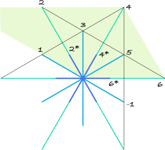
Figure 3: The positive roots $\alpha_{i}$ of $\mathfrak{g}$ are labelled by $\{1,\dots,6\}$. We normalize them so that $\|\alpha_{i}\|^{2}\in\{2,6\}$. With this normalization, $3$ and $4^{*}$ are the fundamental coroots. The positive cone is shaded. The black lines is where the characteristics $\{2\alpha_{2}^{*},2\alpha_{4}^{*},2\alpha_{6}^{*}\}$ take value 2.

5.2.2

Recall that the nilpotent elements in $\mathfrak{g}$ are classified as follows, see [Coll]. First, there are those which are not distinguished, that is, belong to a proper Levi subalgebra. This means they are either 0 or conjugate to a root vector. The corresponding characteristic $h$ is thus either 0 or an element in the dual roots system.

In addition the the principal nilpotent, the Lie algebra $\mathfrak{g}$ has another distinguished class with the characteristic conjugate to

$$h=2\alpha_{4}^{*}=\tfrac{2}{3}\alpha_{4}\,.$$ (166)

This element in plotted in red in Figure 5. For the rest of this section, we fix this $h$. It gives

$$\mathfrak{g}_{2}=\mathfrak{n}_{2}=\textup{span}(e_{2},e_{3},e_{5},e_{6})\,.$$

These are the roots that line on one of the black lines in Figure 3.

5.2.3

We have

$$\mathsf{G}^{h}\cong GL(2)$$

where the $SL(2)$ subgroup corresponds to the root $\alpha_{1}$ and the center corresponds to the coroot $h/2$. As a $\mathsf{G}^{h}$-module,

$$\mathfrak{g}_{2}\cong{\det}^{-1}\otimes S^{3}\mathbb{C}^{2}\,,$$

where $\mathbb{C}^{2}$ is the defining representation of $GL(2)$. The weights of this module can be seen in Figure 5.

Since the center of $GL(2)$ acts with weight $1$ in this representation, the action of $\mathsf{G}^{h}$ on $\mathfrak{g}_{2}$ reduces to action of $PSL(2)$ on

$$\mathbb{P}\left(S^{3}\mathbb{C}^{2}\right)=S^{3}\mathbb{P}^{1}\,,$$

that is, the action on unordered triples of points on $\mathbb{P}^{1}$. This action has an open orbit corresponding to triples of disjoint points, with stabilizer isomorphic to $S(3)$.

The preimage of this open orbit in $\mathfrak{g}_{2}$ is $\mathfrak{g}_{2}^{\circ}$. It corresponds to cubic polynomials in $S^{3}\mathbb{C}^{2}$ with distinct roots. For $e\in\mathfrak{g}_{2}^{\circ}$, the stabilizer is $S(3)$ and the inclusion of the stabilizer

$$S(3)=\mathsf{C}_{\phi}\xrightarrow{\quad\iota\quad}\mathsf{G}^{h}=GL(2)$$ (167)

is the irreducible 2-dimensional representation of $S(3)$.

5.2.4

Since $\mathfrak{g}_{2}=\mathfrak{n}_{2}$, we have $\mathfrak{g}_{2}/\mathfrak{n}_{2}=0$ and hence

$$\mathscr{B}^{e,h}_{1}=\mathsf{G}^{h}/\mathsf{B}^{h}\cong\mathbb{P}^{1}\,.$$

For other elements in $W$, we have

$$\left(s_{6}\mathfrak{n}\right)_{2} =\textup{span}(e_{2},e_{3},e_{5})\,,$$

$$\left(s_{2}\mathfrak{n}\right)_{2} =\textup{span}(e_{5},e_{6})\,,$$

et cetera. In general, the dimension of $(w\mathfrak{n})_{2}$ for various $w$ correspond to the number of positive roots $\alpha$ on lines $\alpha(w^{-1}h)=2$. Three of these lines are plotted in Figure 3, they contain 4, 3, and 2 roots, respectively. Thus counting dimensions as in Corollary 5.3, we see that

$$\mathscr{B}^{e,h}_{w}=\varnothing\,,\quad w\notin\{1,s_{6}\}\,,$$

while

$$\mathscr{B}^{e,h}_{s_{6}}=\textup{3 points}\,.$$

Indeed,

$$\mathbb{P}((s_{6}\mathfrak{n})_{2}^{\circ}) \cong\textup{distinct triples in $S^{3}\mathbb{P}^{1}$ containing $\infty\in\mathbb{P}^{1}$}$$

$$\cong S^{2}\mathbb{A}^{1}\,,$$

and thus

$$\mathscr{B}^{e,h}_{s_{6}}/S(3)\cong(s_{6}\mathfrak{n})_{2}^{\circ}\big{/}\mathsf{B}^{h}\cong\operatorname{pt}/S(2)\,,$$

where we used the identification (164).

5.2.5

Computing the dimensions, we see that $\mathscr{B}^{e}_{1}=\mathbb{P}^{1}$ while

$$\mathscr{B}^{e}_{s_{6}}=\textup{3 copies of $\mathbb{A}^{1}$}\,.$$

Altogether, the Spinger fiber $\mathscr{B}^{e}$ is the configuration of four $\mathbb{P}^{1}$’s, in agreement with the general theory [Slodowy]. See Figure 4, where the arrows indicate the directions of attraction of $q^{h}$ as $q\to 0$.

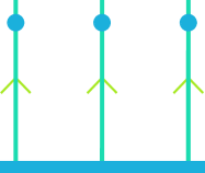
Figure 4: The subregular Springer fiber of type $G_{2}$ is the configuration of $\mathbb{P}^{1}$’s whose dual graph is the Dynkin diagram of type $D_{4}$. The $h$-fixed locus, plotted in thick blue, is the union of $\mathscr{B}_{e}^{1}\cong\mathbb{P}^{1}$ and one point in each of the other components. These 3 components are permuted by $\mathsf{C}_{\phi}\cong S(3)$.

5.3 Spectral projectors and spectral measure

5.3.1

Our next goal is to make explicit the spectral projectors and spectral measure for $e$. We begin with choosing the coordinates $(x_{1},x_{2})$ on $\mathsf{A}$ so that

$$\mathsf{B}^{h}=\left\{\begin{pmatrix}x_{1}&*\\ 0&x_{2}\end{pmatrix}\right\}\subset GL(2)=\mathsf{G}^{h}\,.$$ (168)

The adjoint weights of $\mathsf{A}$ are displayed in Figure 5. The Weyl group $W^{h}\cong S(2)$ acts permuting $x_{1}$ and $x_{2}$.

Figure 5: The characteristic $h$, the adjoint weights of $\mathsf{A}$, and the positive cone. The dotted lines are where $h$ takes values $\pm 2$.

5.3.2

The map (167) satisfies

$$\iota((12))\sim\begin{pmatrix}1\\ &-1\end{pmatrix}\,,\quad\iota((123))\sim\begin{pmatrix}\nu\\ &\nu^{2}\end{pmatrix}\,,\quad\nu=e^{2\pi i/3}\,.$$ (169)

Comparing the characters we conclude that the decomposition (142) takes the form

$$\mathfrak{g}=V^{2}\boxtimes(1+\mathbb{C}^{2})+V^{4}\boxtimes\operatorname{sgn}$$ (170)

where $1$ and $\operatorname{sgn}$ are the two characters of $S(3)$, while $\mathbb{C}^{2}$ is the irreducible 2-dimensional representation. In particular,

$$\operatorname{Slice}_{e}q^{-1}\mathfrak{g} =q^{-2}(1+\mathbb{C}^{2})+q^{-3}\operatorname{sgn}\,,$$

$$\mathfrak{c}_{e} =q(1+\mathbb{C}^{2})+q^{2}\operatorname{sgn}\,,$$ (171)

as $\widehat{\mathsf{C}}_{e}$-modules. We conclude

$$\Psi_{e}\Big{|}_{q^{h/2}S(3)}=\Psi\Big{(}(q^{-2}-q)(\mathbb{C}^{2}+1)+(q^{-3}-q^{2})\operatorname{sgn}-4q^{-1}\Big{)}\,.$$ (172)

5.3.3

The spectral projectors $\mathscr{P}_{\pm}$ are given by integration along the Spinger fibers as in (125). They take a function $f(x_{1},x_{2})$ on the torus $\mathsf{A}$, viewed as K-theory class on $\mathscr{B}_{e}$ to a conjugation-invariant function on $S(3)$. The difference between $\mathscr{P}_{\pm}$ is in the identification of $K_{\mathsf{G}}(\mathscr{B})$ with functions on the torus $\mathscr{A}$. Since opposite Borel subgroups are used for this identification, we have

$$\mathscr{P}_{+}=\mathscr{P}_{-}\circ w_{0}\,,\quad w_{0}(x_{1},x_{2})=(x_{1}^{-1},x_{2}^{-1})\,.$$

Here $w_{0}$ is the longest element of the Weyl group.

By stratification and equivariant localization, the integral over $\mathscr{B}^{e}$ is reduced to integrals over $\mathscr{B}^{h,e}_{w}$ for $w=1,s_{6}$, giving the decomposition

$$\mathscr{P}_{+}=\mathscr{P}_{+,1}+\mathscr{P}_{+,s_{6}}\,.$$

We deal with them separately, starting with $w=1$.

5.3.4

Restricted to $\mathscr{B}^{h}_{1}$, the virtual tangent bundle to $\mathscr{B}_{e}$ is induced from the $\mathsf{B}^{h}$-module

$$(1-q^{-1})\mathfrak{n}^{\vee} =(1-q^{-1})(\mathfrak{g}_{-4}+\mathfrak{g}_{-2})+(1-q^{-1})x_{2}/x_{1}$$ (173)

$$=\underbrace{(1-q^{-1})(\mathfrak{g}_{-4}+\mathfrak{g}_{-2})+q^{-1}(2-\mathfrak{g}_{0})}_{\textup{trivial bundle $V_{0}$}}+\underbrace{x_{2}/x_{1}+q^{-1}x_{1}/x_{2}}_{T^{*}\mathbb{P}^{1}}\,.$$

We observe that last two terms give the cotangent bundle to $\mathsf{B}^{h,e}_{1}\cong\mathbb{P}^{1}$, while the remaining terms, being $\mathsf{G}^{h}$-modules, induce a trivial virtual bundle $V_{0}$ over $\mathbb{P}^{1}$ with the corresponding action. Computing their $S(3)$-characters, we conclude

$$V_{0}=-q^{-3}\operatorname{sgn}-q^{-2}(1+\mathbb{C}^{2})+2q^{-1}\,.$$

Therefore

$$\mathscr{P}_{+,1}\,f\Big{|}_{q^{h/2}S(3)}=\Psi(V_{0})\,\operatorname{\mathbf{D}}f\Big{|}_{q^{h/2}S(3)}$$

where

$$\operatorname{\mathbf{D}}f(x_{1},x_{2}) =\chi(f\otimes\psi(T^{*}\mathbb{P}^{1}))$$

$$=(1+(12))Z(x_{1}/x_{2})f(x_{1},x_{2})\,.$$ (174)

The result in (174) is interpreted geometrically as an element of $K_{GL(2)}(\operatorname{pt})$, which we subsequently restrict to $q^{h/2}S(3)$.

Collecting all terms above, we obtain

$$\Psi_{e}\left(\mathscr{P}_{+,1}f_{1}\right)\left(\mathscr{P}_{-,1}f_{2}\right)\Big{|}_{q^{h/2}S(3)}=\left.\frac{\operatorname{\mathbf{D}}f_{1}(x_{1},x_{2})\,\operatorname{\mathbf{D}}f_{2}(x_{1}^{-1},x_{2}^{-1})}{Z(q^{2}(1+\mathbb{C}^{2})+q^{3}\operatorname{sgn})}\right|_{q^{h/2}S(3)}\,.$$ (175)

5.3.5

Note that because of the pole of $Z(x_{1}/x_{2})$ at $x_{1}=x_{2}$, the value of (174) at $q^{h/2}$, that is, at $(x_{1},x_{2})=(q,q)$, involves the derivatives of $f$ at this point, as well as the subleading term in the expansion of $Z$ at the pole.

Concretely, if

$$Z(x)=\frac{z_{-1}}{1-x^{-1}}+z_{0}+\dots$$

then

$$\operatorname{\mathbf{D}}f(x_{1},x_{2})\Big{|}_{x_{1}=x_{2}}=(z_{-1}+2z_{0})f(x_{1},x_{1})+z_{-1}\left.\left(x_{1}\frac{\partial}{\partial x_{1}}-x_{2}\frac{\partial}{\partial x_{2}}\right)f\right|_{x_{1}=x_{2}}\,.$$

5.3.6

We now consider $\mathscr{B}^{h,e}_{s_{6}}$, which consists of $3$ points permuted by $S(3)$. Since this is a permutation representation, the character of $(123)$ vanishes, the character of $(12)$ equals the contribution of unique point fixed by this transposition, while the character of identity is 3 times the contribution of a single point.

As a concrete nilpotent element $e$ we may take

$$e=e_{2}+e_{5}\,,$$

where the labeling of the roots is an in Figure 3, the normalization of the root vectors being immaterial. This belongs to $\mathfrak{g}_{2}^{\circ}$, is fixed by

$$\mathsf{A}^{e}=\left\{\begin{pmatrix}\varepsilon&0\\ 0&1\end{pmatrix}\right\}\,,\quad\varepsilon=\pm 1\,.$$ (176)

and is contained in $s_{6}\mathfrak{n}$, see Figure 6.

Figure 6: Same as in Figure 5 but now $s_{6}\mathfrak{n}\in\mathscr{B}^{e}$ is shaded.

The reflection $s_{6}$ acts by

$$s_{6}\cdot(x_{1},x_{2})=(x_{1},x_{1}/x_{2})$$

and we have to apply $s_{6}$ to both the K-theory class $f$ and to the character of the virtual normal bundle (173) to compute the contribution of the point $s_{6}\mathfrak{n}\in\mathscr{B}^{e,h}_{s_{6}}$. We obtain

$$(1-q^{-1})T\mathscr{B}\Big{|}_{s_{6}\mathfrak{n}} =2(q^{-1}-q^{-2})+(q-q^{-3})\varepsilon\,.$$

$$=V_{0}\Big{|}_{S(2)}+\varepsilon(q+q^{-2})\,.$$ (177)

Therefore

$$\mathscr{P}_{+,s_{6}} f\Big{|}_{q^{h/2}} =3\Psi(V_{0})Z(q^{2})f(q,1)\,,$$ (178)

$$\mathscr{P}_{+,s_{6}} f\Big{|}_{q^{h/2}(12)} =\Psi(V_{0})Z(-q^{2})f(-q,-1)\,,$$ (179)

$$\mathscr{P}_{+,s_{6}} f\Big{|}_{q^{h/2}(123)} =0\,.$$ (180)

5.3.7

We now have all the data needed to express the contribution of the subregular nilpotent $e$ to the spectrum. The contributions consist of 3 isolated points corresponding to the conjugacy classes of $S(3)$.

The identity $1\in S(3)$ corresponds to the point

$$Wq^{h/2}=W(q,q)\in\mathsf{A}/W=\operatorname{Spec}\mathbf{sH}$$

and contributes

$$\|\delta_{W(q,q)}f\|_{\Psi}^{2}=\frac{1}{6}\frac{1}{Z(q^{2})^{3}Z(q^{3})}\left|\operatorname{\mathbf{D}}f\Big{|}_{(q,q)}+3Z(q^{2})f(q,1)\right|^{2}\,,$$ (181)

to the spectrum, where $\delta_{W(q,q)}$ is the spectral projector. The prefactor $\frac{1}{6}$ comes from the Haar measure on $S(3)$ and the difference $3Z(q^{2})f(q,1)$ between (181) and (175) is the contribution of (178)  .

The transposition $(12)\in S(3)$ corresponds to the point $(-q,q)\in\operatorname{Spec}\mathbf{sH}$ and it contributes

$$\|\delta_{W(-q,q)}f\|_{\Psi}^{2}=\frac{1}{2}\frac{\left|Z(-1)(f(-q,q)+f(q,-q))+Z(-q^{2})f(-q,-1)\right|^{2}}{Z(q^{2})^{2}Z(-q^{2})Z(-q^{3})}\,.$$ (182)

Finally, the cycle $(123)$ corresponds to the point $(q\nu,q\nu^{2})$ where $\nu=e^{2\pi i/3}$, and it contributes

$$\|\delta_{W(q\nu,q\nu^{2})}f\|_{\Psi}^{2}=\frac{1}{3}\frac{\left|Z(\nu^{-1})f(q\nu,q\nu^{2})+Z(\nu)f(q\nu^{2},q\nu)\right|^{2}}{Z(q^{2})Z(q^{2}\nu)Z(q^{2}\nu^{2})Z(q^{3})}\,.$$ (183)

5.3.8

In the number field situation, that is, in cohomology, only the point (181) survives and becomes the point

$$\tfrac{1}{2}h=\alpha^{*}_{4}=(1,1)\in\operatorname{Lie}\mathsf{A}/W\,.$$

It is instructive to compare the results with Landlands’ computation.

The additive analog of the operator (174) is the operator

$$\operatorname{\mathbf{D}_{a}}f=(1+(12))\,\xi(x_{1}-x_{2})f(x_{1},x_{2})\,.$$ (184)

where

$$\xi(x)=-\frac{1}{x}+a+\dots\,,$$

in the notations introduces at the bottom of page 186 in [L]. This means that

$$\operatorname{\mathbf{D}_{a}}f\Big{|}_{x_{1}=x_{2}}=-(\partial_{1}-\partial_{2})f(x_{1},x_{1})+2af(x_{1},x_{1})\,.$$

Therefore

$$\|\delta_{W(1,1)}f\|_{\Psi}^{2}=\frac{1}{6}\frac{\left|(\partial_{1}-\partial_{2})f(1,1)-2af(1,1)-3\xi(2)f(1,0)\right|^{2}}{\xi(2)^{3}\xi(3)}\,,$$ (185)

where we have changed the sign under the absolute value sign to ease the comparison with the matrix in Figure 7.

Figure 7: The spectral projector for the discrete spectrum of $G_{2}$ reproduced from page 195 of [L]. The point $\rho$, which corresponds to $\rho^{\vee}$ in our notations, is the contribution of the regular nilpotent considered in Section 3.6.

To match the coordinates with Langland’s coordinates, we note that Langlands’ roots $\beta_{i}$ are our dual roots $\alpha_{i}^{*}$, see the illustration on on page 181 of [L]. In particular,

$$\beta_{4}=(1,1)\,,\quad\beta_{2}=s_{6}\beta_{4}=(1,0)\,,$$

and

$$\beta_{1}=2\beta_{2}-\beta_{4}=(1,-1)\,.$$

Since the derivative $D_{1}$ used by Langlands is the derivative in the direction of $\beta_{1}$, we conclude

$$D_{1}=\partial_{1}-\partial_{2}\,,$$

completing the match.

Appendix A Appendix

A.1 Group cohomology

A.1.1

The cohomology of a complex algebraic group $\mathsf{G}$ with coefficients in a representation $V$ is defined by

$$H^{i}(\mathsf{G},V)=\operatorname{Ext}^{i}_{\mathsf{G}}(\mathbb{C},V)\,,$$

where $\mathbb{C}$ is trivial representation and Ext’s are computed in the category of algebraic $\mathsf{G}$-modules. These are the derived functors of $\mathsf{G}$-invariants

$$H^{0}(\mathsf{G},V)=V^{\mathsf{G}}\,.$$

They may be computed using the usual cochain complex, see e.g. [FF], in which the terms are given by morphisms $\mathsf{G}^{\times n}\to V$ of algebraic varieties.

A.1.2

We define

$$\chi(\mathsf{G},V)=\sum_{i}(-1)^{i}H^{i}(\mathsf{G},V)\,.$$ (186)

This is linear in the $K_{\mathsf{G}}(\operatorname{pt})$-class of $V$ by the long exact sequence of cohomology.

A.1.3

For a group extension

$$1\to\mathsf{G}_{1}\to\mathsf{G}\to\mathsf{G}_{2}\to 1\,,$$

we have

$$\chi(\mathsf{G},V)=\chi(\mathsf{G}_{2},\chi(\mathsf{G}_{1},V))$$ (187)

by the spectral sequence for derived functors of

$$V^{\mathsf{G}}=\left(V^{\mathsf{G}_{1}}\right)^{\mathsf{G}_{2}}\,.$$

Formula (187) reduces the computation of $\chi(\mathsf{G},V)$ to that for the unipotent radical and the reductive quotient in (48).

A.1.4

We have (essentially by definition)

$$\textup{$\mathsf{G}$ is reductive}\,\Leftrightarrow H^{>0}(\mathsf{G},\,\cdot\,)=0\,,$$

and if $\mathsf{U}$ is a unipotent group then

$${H}^{\raisebox{1.42262pt}{$\scriptscriptstyle\bullet$}}(\mathsf{U},V)={H}^{\raisebox{1.42262pt}{$\scriptscriptstyle\bullet$}}(\mathfrak{u},V)\,,\quad\mathfrak{u}=\operatorname{Lie}\mathsf{U}\,,$$ (188)

as a consequence of the Hochschild-Mostow spectral sequence, see [FF], Section 1.§3.

A.1.5

We recall that Lie algebra cohomology in (188) is succinctly computed by the Chevalley-Eilenberg complex

$${H}^{\raisebox{1.42262pt}{$\scriptscriptstyle\bullet$}}(\mathfrak{u},V)={H}^{\raisebox{1.42262pt}{$\scriptscriptstyle\bullet$}}\left(V\to V\otimes\mathfrak{u}^{\vee}\to V\otimes\Lambda^{2}\mathfrak{u}^{\vee}\to\dots\right)\,.$$ (189)

A.2 Cohomologically proper actions

A.2.1

Consider an action-preserving map

$$(\mathsf{G}_{1},\mathsf{X}_{1})\xrightarrow{\quad(f_{\mathsf{G}},f_{\mathsf{X}})\quad}(\mathsf{G}_{2},\mathsf{X}_{2})$$ (190)

with $f_{\mathsf{G}}$ surjective. It is cohomologically proper if ${\mathsf{R}}^{\raisebox{1.42262pt}{$\scriptscriptstyle\bullet$}}(f_{\mathsf{G}},f_{\mathsf{X}})_{*}\mathscr{F}$ is a bounded complex of coherent sheaves for any $\mathscr{F}\in\operatorname{Coh}_{\mathsf{G}_{1}}(\mathsf{X}_{1})$. Here

$$R^{0}(f_{\mathsf{G}},f_{\mathsf{X}})_{*}\mathscr{F}=\left(f_{\mathsf{X},*}\mathscr{F}\right)^{\ker f_{\mathsf{G}}}\,.$$

Obviously, cohomological proper maps are closed under composition and a proper map is cohomologically proper.

A.2.2

By definition, an action of an algebraic group $\mathsf{G}$ on a scheme $\mathsf{X}$ is cohomologically proper if the canonical map

$$(\mathsf{G},\mathsf{X})\to(\{1\},\operatorname{pt})$$

is cohomologically proper. In this case, we also say that the quotient stack $\mathsf{X}/\mathsf{G}$ is cohomologically proper.

A.2.3

A nontrivial example of a cohomologically proper map is given by the following

Proposition A.1.

If the map $f_{\mathsf{X}}$ in (190) is affine, $\ker f_{\mathsf{G}}$ is reductive, and

$$(f_{\mathsf{X},*}\mathscr{O}_{\mathsf{X}_{1}})^{\ker f_{\mathsf{G}}}=\mathscr{O}_{\mathsf{X}_{2}}$$

then (190) is cohomologically proper

Proof.

It suffices to prove that for a finitely generated algebra $\mathscr{A}$ with an action of a reductive group $\mathsf{G}$

$$\dim\mathscr{A}^{\mathsf{G}}<\infty\Leftrightarrow\forall V\,,\dim(\mathscr{A}\otimes V)^{\mathsf{G}}<\infty$$

where $V$ ranges over finite-dimensional $\mathsf{G}$-modules.

Highest weights vectors of irreducible $\mathsf{G}$-submodules in $\mathscr{A}$ span the graded algebra

$$\mathscr{A}^{\mathsf{U}}=\bigoplus_{\lambda\in\,\textup{dominant weights}}\mathscr{A}^{\mathsf{U}}_{\lambda}\,,$$ (191)

where $\mathsf{U}\subset\mathsf{G}$ is a maximal unipotent subgroup. This algebra is finitely generated by Theorem 3.13 in [VinPop]. Therefore

$$\dim\mathscr{A}^{\mathsf{U}}_{0}<\infty\Leftrightarrow\forall\lambda\,,\dim\mathscr{A}_{\lambda}^{\mathsf{U}}<\infty\,,$$

as was to be shown. ∎

A.2.4

Proposition A.2.

The conclusion of Proposition A.1 also holds for $\ker f_{\mathsf{G}}=\mathbb{G}_{\mathbf{a}}$.

Proof.

Suffices to prove that

$$\dim H^{1}(\mathbb{G}_{\mathbf{a}},\mathscr{A})\leq\dim H^{0}(\mathbb{G}_{\mathbf{a}},\mathscr{A})\,,$$

for any algebraic module $\mathscr{A}$, that is, any module of the form

$$\mathscr{A}=\bigcup\mathscr{A}_{n}\,,\quad\dim\mathscr{A}_{n}<\infty\,.$$

Here $\mathscr{A}_{n}$ is a finite-dimensional vector space with a nilpotent operator, for which $H^{0}$ and $H^{1}$ are the kernel and the cokernel, respectively. Therefore,

$$\dim H^{1}(\mathbb{G}_{\mathbf{a}},\mathscr{A})\leq\lim\dim H^{1}(\mathbb{G}_{\mathbf{a}},\mathscr{A}_{n})=\lim\dim H^{0}(\mathbb{G}_{\mathbf{a}},\mathscr{A}_{n})=\dim H^{0}(\mathbb{G}_{\mathbf{a}},\mathscr{A})\,.$$

∎

Remark A.1.

For a general unipotent group, the conclusion of Proposition A.1 fails, which has to do with the fact that a quotient of an affine variety by a unipotent group is, in general, only quasiaffine. As a simplest example, one can take the maps

$$\lx@xy@svg{\hbox{\raise 0.0pt\hbox{\kern 38.50824pt\hbox{\ignorespaces\ignorespaces\ignorespaces\hbox{\vtop{\kern 0.0pt\offinterlineskip\halign{\entry@#!@&&\entry@@#!@\cr&&\\&\crcr}}}\ignorespaces{\hbox{\kern-38.50824pt\raise 0.0pt\hbox{\hbox{\kern 0.0pt\raise 0.0pt\hbox{\hbox{\kern 3.0pt\raise 0.0pt\hbox{$\textstyle{U\backslash SL(2,\mathbb{C})/U\ignorespaces\ignorespaces\ignorespaces\ignorespaces\ignorespaces\ignorespaces\ignorespaces\ignorespaces}$}}}}}}}\ignorespaces\ignorespaces\ignorespaces\ignorespaces{}{\hbox{\lx@xy@droprule}}\ignorespaces{\hbox{\kern 99.73047pt\raise 0.0pt\hbox{\hbox{\kern 0.0pt\raise 0.0pt\hbox{\lx@xy@tip{1}\lx@xy@tip{-1}}}}}}{\hbox{\lx@xy@droprule}}{\hbox{\lx@xy@droprule}}\ignorespaces\ignorespaces\ignorespaces{}\ignorespaces\ignorespaces{\hbox{\lx@xy@drawline@}}\ignorespaces{\hbox{\kern 62.50824pt\raise-35.3159pt\hbox{\hbox{\kern 0.0pt\raise 0.0pt\hbox{\lx@xy@tip{1}\lx@xy@tip{-1}}}}}}\ignorespaces\ignorespaces{\hbox{\lx@xy@drawline@}}\ignorespaces{\hbox{\lx@xy@drawline@}}{\hbox{\kern 66.11935pt\raise 0.0pt\hbox{\hbox{\kern 0.0pt\raise 0.0pt\hbox{\hbox{\kern 3.0pt\raise 0.0pt\hbox{$\textstyle{}$}}}}}}}{\hbox{\kern 99.73047pt\raise 0.0pt\hbox{\hbox{\kern 0.0pt\raise 0.0pt\hbox{\hbox{\kern 3.0pt\raise 0.0pt\hbox{$\textstyle{U\backslash(\mathbb{C}^{2}\setminus\{0\})\ignorespaces\ignorespaces\ignorespaces\ignorespaces}$}}}}}}}\ignorespaces\ignorespaces\ignorespaces{}\ignorespaces\ignorespaces{\hbox{\lx@xy@drawline@}}\ignorespaces{\hbox{\kern 75.73047pt\raise-34.91562pt\hbox{\hbox{\kern 0.0pt\raise 0.0pt\hbox{\lx@xy@tip{1}\lx@xy@tip{-1}}}}}}\ignorespaces\ignorespaces{\hbox{\lx@xy@drawline@}}\ignorespaces{\hbox{\lx@xy@drawline@}}{\hbox{\kern-3.0pt\raise-39.0411pt\hbox{\hbox{\kern 0.0pt\raise 0.0pt\hbox{\hbox{\kern 3.0pt\raise 0.0pt\hbox{$\textstyle{}$}}}}}}}{\hbox{\kern 62.50824pt\raise-39.0411pt\hbox{\hbox{\kern 0.0pt\raise 0.0pt\hbox{\hbox{\kern 3.0pt\raise 0.0pt\hbox{$\textstyle{\mathbb{C}}$}}}}}}}\ignorespaces}}}}\ignorespaces\,, \textstyle{U\backslash SL(2,\mathbb{C})/U\ignorespaces\ignorespaces\ignorespaces\ignorespaces\ignorespaces\ignorespaces\ignorespaces\ignorespaces} \textstyle{U\backslash(\mathbb{C}^{2}\setminus\{0\})\ignorespaces\ignorespaces\ignorespaces\ignorespaces} \textstyle{\mathbb{C}} \textstyle{U\backslash SL(2,\mathbb{C})/U\ignorespaces\ignorespaces\ignorespaces\ignorespaces\ignorespaces\ignorespaces\ignorespaces\ignorespaces} \textstyle{U\backslash(\mathbb{C}^{2}\setminus\{0\})\ignorespaces\ignorespaces\ignorespaces\ignorespaces} \textstyle{\mathbb{C}}$$ (192)

where $U$ is a maximal unipotent subgroup.

A.3 Flag varieties and Springer fibers

A.3.1

Let $\mathsf{G}$ be a complex semisimple Lie group with $\operatorname{Lie}(\mathsf{G})=\mathfrak{g}$. Choose a Borel subgroup $\mathsf{B}\subset\mathsf{G}$. We have

$$\mathsf{B}=\mathsf{A}\ltimes\mathsf{U}$$

where $\mathsf{U}$ is the unipotent radical and $\mathsf{A}$ a maximal torus. We denote

$$\mathfrak{b}=\operatorname{Lie}(\mathsf{B})\,,\quad\mathfrak{n}=\operatorname{Lie}\mathsf{U}\,.$$

We denote by $r$ the rank of $\mathfrak{g}$ .

A.3.2

The flag variety

$$\mathscr{B}\overset{\textup{\tiny def}}{=}\mathsf{G}/\mathsf{B}=\{\mathfrak{b}^{\prime}\subset\mathfrak{g}\}=\{\mathfrak{n}^{\prime}\subset\mathfrak{g}\}$$

may be seen as parametrizing Borel subalgebras $\mathfrak{b}^{\prime}\subset\mathfrak{g}$, or the corresponding nilpotent subalgebras $\mathfrak{n}^{\prime}=[\mathfrak{b}^{\prime},\mathfrak{b}^{\prime}]$, with the adjoint action of $\mathsf{G}$. Further,

$$T^{*}\mathscr{B}=\{(e,\mathfrak{n}^{\prime}),e\in\mathfrak{n}^{\prime}\}\,.$$ (193)

Here $e\in\mathfrak{g}$ is a nilpotent element. The map

$$\mu:T^{*}\mathscr{B}\owns(e,\mathfrak{n}^{\prime})\mapsto e\in\mathfrak{g}$$ (194)

becomes the moment map upon the identification $\mathfrak{g}\cong\mathfrak{g}^{*}$ given by an invariant bilinear form. We will always treat this map $\mathbb{C}^{\times}_{q}$-equivariantly, where $\mathbb{C}^{\times}_{q}$ acts by $e\mapsto q^{-1}e$.

A.3.3

For any semisimple $h\in\mathfrak{g}$ we have

$$\mathscr{B}^{h}=\bigsqcup_{w\in W^{h}\backslash W}\mathsf{G}^{h}\,w\,\mathfrak{n}\,,$$ (195)

where $w$ ranges over coset representatives of minimal length, that is, such that

$$w^{-1}\mathsf{B}^{h}w\subset\mathsf{B}\,.$$

Each component in (195) parametrizes $h$-stable maximal nilpotent subalgebras $\mathfrak{n}^{\prime}$ with the same dimensions of the graded components as $w\cdot\mathfrak{n}$.

A.3.4

If $e\in\mathfrak{g}$ is a nilpotent element then

$$\mathscr{B}^{e}=\mu^{-1}(e)$$ (196)

is the Springer fiber of $e$. Being the zero locus of a vector field, it has a natural derived scheme structure with the virtual tangent bundle $(1-q^{-1})T\mathscr{B}$.

A.4 Normalization of measures

A.4.1

While the spectral decomposition is obviously insensitive to the precise normalization of the measures, it is worth mentioning briefly the different choices that contribute to the normalization in Langlands’ formula (5).

A.4.2

The Haar measure on $\mathsf{G}(\mathbb{A})$ is the pushforward of the measure

$$d_{\textup{Haar}}(k)\times|a|^{-2\rho}d_{\textup{Haar}}(a)\times d_{\textup{Haar}}(u)$$ (197)

under the Iwasawa factorization map

$$\mathsf{K}\times\mathsf{A}\times\mathsf{U}\to\mathsf{G}\,.$$

There is a canonical way to normalize the first and the last factor in (197) by

$$\operatorname{vol}(\mathsf{K})=\operatorname{vol}(\mathsf{U}(\mathbb{A})/\mathsf{U}(\mathbb{F}))=1\,.$$ (198)

Instead of the Iwasawa factorization, one can fix a measure on the Borel subgroup $\mathsf{B}=\mathsf{A}\mathsf{U}$ and normalize the volume of the flag manifold $\operatorname{vol}(\mathsf{G}(\mathbb{A})/\mathsf{B}(\mathbb{A}))=1$. This is a more natural and a more uniform normalization when working with Eisenstein series and constant terms.

A.4.3

Because the group $\mathsf{U}$ is unipotent, the measure $d_{\textup{Haar}}(u)$ normalized as in (198) equals the the Tamagawa measure

$$d_{\textup{Haar}}(u)=d_{\textup{\raisebox{-2.84526pt}{\includegraphics[height=10.0pt]{Tama.png}}}}(u)\,.$$

Recall that e.g. for the additive group of a number field we have

$$\mathbb{A}/\mathbb{F}=\prod_{\textup{finite $p$}}\mathscr{O}_{p}\times\left(\left.\prod_{p|\infty}F_{p}\right/\mathscr{O}_{\mathbb{F}}\right)$$

and the Tamagawa measure of $\mathbb{A}/\mathbb{F}$ equals the square root of the ratio of the absolute value of discriminant (from the infinite places) and norms of the differents (from the finite places), hence $=1$. It is through the relation

$$\prod_{\textup{finite $p$}}\operatorname{vol}(\mathscr{O}_{p})=\left|\textup{discr}\mathscr{O}_{F}\right|^{-1/2}\,,$$

that the discriminant factor in completed zeta functions appears as product of local contribution in (5).

A.4.4

For $\mathsf{A}$ factor in (197), we take the Tamagawa measure. Since $\mathsf{A}\cong GL(1)^{r}$, it suffices to discuss the multiplicative group $GL(1)$. Since

$$H^{0}(GL(1,\overline{F}),\mathscr{O}^{\times})/\overline{F}^{\times}=\mathbb{Z}\,,\quad H^{1}(GL(1,\overline{F}),\mathscr{O}^{\times})=0\,,$$

where $\mathbb{Z}$ has the trivial Galois group action, we have [Ono]

$$d_{GL(1),\textup{\raisebox{-2.84526pt}{\includegraphics[height=10.0pt]{Tama.png}}}}(x)=\prod_{\textup{finite $p$}}\frac{1}{1-p^{-1}}\frac{dx}{\,\,\,|x|_{p}}\times\prod_{p|\infty}\frac{dx}{\,\,\,|x|_{p}}\,.$$

A.4.5

Since we consider only unramified characters of $\mathsf{A}$, we effectively work with the pushforward under the norm map

$$d_{\mathscr{Q},\textup{\raisebox{-2.84526pt}{\includegraphics[height=10.0pt]{Tama.png}}}} =\left(GL(1,\mathbb{A})\xrightarrow{\quad\|\,\cdot\,\|\quad}\mathscr{Q}\right)_{*}d_{GL(1),\textup{\raisebox{-2.84526pt}{\includegraphics[height=10.0pt]{Tama.png}}}}$$

$$=\big{(}\operatorname{Res}_{s=1}\xi(s)ds\big{)}\,\frac{dq}{q}\,.$$ (199)

Here the second line follows the presentation of $\xi(s)$ as an integral with respect to $GL(1,\mathbb{A})$ as in Tate’s thesis [Tate]. In the case when $\mathscr{Q}$ is discrete, the measure $\frac{dq}{q}$ is the counting measure.

A.4.6

By the formula (23) we have

$$\operatorname{Res}_{s=1}\xi(s)ds=\begin{cases}\frac{1}{\ln q}\,\textup{\small\cursive z}\,,&\operatorname{char}\mathbb{F}>0\\ \textup{\small\cursive z}\,,&\operatorname{char}\mathbb{F}=0\,.\end{cases}$$ (200)

Thus the natural measure on the dual group

$$\mathscr{Q}^{\vee}=\mathbb{C}\left/\frac{2\pi i}{\ln q}\,\mathbb{Z}\right.\,,$$

where $q=1$ in the number field case in (1), is

$$d_{\mathscr{Q}^{\vee},\textup{\raisebox{-2.84526pt}{\includegraphics[height=10.0pt]{Tama.png}}}}(s)=\frac{1}{2\pi i\textup{\small\cursive z}}ds\,,$$ (201)

in all cases. Note, in particular, this is correctly normalized in the $q\to 1$ limit.

This is the how the Haar measure (121) should be normalized to reproduce actual $L^{2}$-norms in (5).

A.4.7

In [Lvol], Langlands compares the above normalization of the Haar measure on $\mathsf{G}(\mathbb{A})$ with the Tamagawa measure for $\mathsf{G}(\mathbb{A})$. This amount to computing the Tamagawa volumes of the flag manifolds.

In the number field case, for the nonarchimedian places, point counts in flag manifolds give

$$\prod_{p\,\nmid\,\infty}\operatorname{vol}_{\textup{\raisebox{-2.84526pt}{\includegraphics[height=10.0pt]{Tama.png}}}}(\mathsf{G}(\mathbb{F}_{p})/\mathsf{B}(\mathbb{F}_{p}))=\left|\textup{discr}\mathscr{O}_{F}\right|^{-\frac{1}{2}\dim\mathsf{G}/\mathsf{B}}\prod_{i=1}^{r}\zeta_{\mathbb{F}}(m_{i}+1)^{-1}\,,$$

where $m_{i}$ are the exponents of $\mathsf{G}$, with a similar answer in the function field case. One should bear in mind that $H^{1}(\mathsf{G}/\mathsf{B},\mathscr{O}^{\times})=\mathbb{Z}^{r}$ with a trivial Galois action, which multiplies the point counts by $(1-p^{-1})^{r}$.

The archimedian contribution, concretely the volume of the flag manifold computed on the big Bruhat cell, Langlands interprets as a particular value of the Gindikin-Karpelevich formula. Altogether, the proportionality constant is the residue at the regular nilpotent discussed in Section 3.6. Since the residue of the Eisenstein series at that point is a constant function on $\mathsf{G}$, Langlands computes the Tamagawa volume of $\mathsf{G}(\mathbb{F})\backslash\mathsf{G}(\mathbb{A})$.

References

AtiyahMichael FrancisElliptic operators and compact groupsLecture Notes in Mathematics, Vol. 401Springer-Verlag, Berlin-New York1974ii+93@book{Atiyah, author = {Atiyah, Michael Francis}, title = {Elliptic operators and compact groups}, series = {Lecture Notes in Mathematics, Vol. 401}, publisher = {Springer-Verlag, Berlin-New York}, date = {1974}, pages = {ii+93}} BerlineNicoleVergneMichΓ¨leThe chern character of a transversally elliptic symbol and the equivariant indexInvent. Math.12419961-311–49@article{BerlVerg, author = {Berline, Nicole}, author = {Vergne, Mich\`ele}, title = {The Chern character of a transversally elliptic symbol and the equivariant index}, journal = {Invent. Math.}, volume = {124}, date = {1996}, number = {1-3}, pages = {11–49}} BiaΕ‚ynicki-BirulaA.Some theorems on actions of algebraic groupsAnn. of Math. (2)981973480–497@article{BB, author = {Bia\l{}ynicki-Birula, A.}, title = {Some theorems on actions of algebraic groups}, journal = {Ann. of Math. (2)}, volume = {98}, date = {1973}, pages = {480–497}} BogomolovF. A.Holomorphic tensors and vector bundles on projective manifoldsIzv. Akad. Nauk SSSR Ser. Mat.4219786@article{Bogo, author = {Bogomolov, F. A.}, title = {Holomorphic tensors and vector bundles on projective manifolds}, journal = {Izv. Akad. Nauk SSSR Ser. Mat.}, volume = {42}, date = {1978}, number = {6}} BravermanMaximIndex theorem for equivariant dirac operators on noncompact manifoldsK𝐾K-Theory272002161–101@article{BravM, author = {Braverman, Maxim}, title = {Index theorem for equivariant Dirac operators on noncompact manifolds}, journal = {$K$-Theory}, volume = {27}, date = {2002}, number = {1}, pages = {61–101}} CollingwoodDavid H.McGovernWilliam M.Nilpotent orbits in semisimple lie algebrasVan Nostrand Reinhold Mathematics SeriesVan Nostrand Reinhold Co., New York1993xiv+186@book{Coll, author = {Collingwood, David H.}, author = {McGovern, William M.}, title = {Nilpotent orbits in semisimple Lie algebras}, series = {Van Nostrand Reinhold Mathematics Series}, publisher = {Van Nostrand Reinhold Co., New York}, date = {1993}, pages = {xiv+186}} De ConciniC.LusztigG.ProcesiC.Homology of the zero-set of a nilpotent vector field on a flag manifoldJ. Amer. Math. Soc.11988115–34@article{dCLP, author = {De Concini, C.}, author = {Lusztig, G.}, author = {Procesi, C.}, title = {Homology of the zero-set of a nilpotent vector field on a flag manifold}, journal = {J. Amer. Math. Soc.}, volume = {1}, date = {1988}, number = {1}, pages = {15–34}} De ConciniC.ProcesiC.VergneM.The infinitesimal indexJ. Inst. Math. Jussieu1220132297–334@article{CPV2, author = {De Concini, C.}, author = {Procesi, C.}, author = {Vergne, M.}, title = {The infinitesimal index}, journal = {J. Inst. Math. Jussieu}, volume = {12}, date = {2013}, number = {2}, pages = {297–334}} De ConciniC.ProcesiC.VergneM.Box splines and the equivariant index theoremJ. Inst. Math. Jussieu1220133503–544@article{CPV, author = {De Concini, C.}, author = {Procesi, C.}, author = {Vergne, M.}, title = {Box splines and the equivariant index theorem}, journal = {J. Inst. Math. Jussieu}, volume = {12}, date = {2013}, number = {3}, pages = {503–544}} FeiginB. L.FuchsD. B.Cohomologies of lie groups and lie algebrastitle={Lie groups and Lie algebras, II}, series={Encyclopaedia Math. Sci.}, volume={21}, publisher={Springer, Berlin}, 2000125–223@article{FF, author = {Feigin, B. L.}, author = {Fuchs, D. B.}, title = {Cohomologies of Lie groups and Lie algebras}, conference = {title={Lie groups and Lie algebras, II}, }, book = {series={Encyclopaedia Math. Sci.}, volume={21}, publisher={Springer, Berlin}, }, date = {2000}, pages = {125–223}} Halpern-LeistnerDanielThe derived category of a git quotientJ. Amer. Math. Soc.2820153871–912@article{DHL, author = {Halpern-Leistner, Daniel}, title = {The derived category of a GIT quotient}, journal = {J. Amer. Math. Soc.}, volume = {28}, date = {2015}, number = {3}, pages = {871–912}}
• [12] D.Β Halpern-Leistner, A categorification of the Atiyah-Bott localization formula, available from math.cornell.edu/Β danielhl.
• [13] Marcelo De Martino, Volker Heiermann, Eric Opdam, On the unramified spherical automorphic spectrum, arXiv:1512.08566 (new version v4 in preparation)
• HesselinkWim H.Uniform instability in reductive groupsJ. Reine Angew. Math.303(304)197874–96@article{Hess, author = {Hesselink, Wim H.}, title = {Uniform instability in reductive groups}, journal = {J. Reine Angew. Math.}, volume = {303(304)}, date = {1978}, pages = {74–96}} KazhdanDavidLusztigGeorgeProof of the deligne-langlands conjecture for hecke algebrasInvent. Math.8719871153–215@article{KL, author = {Kazhdan, David}, author = {Lusztig, George}, title = {Proof of the Deligne-Langlands conjecture for Hecke algebras}, journal = {Invent. Math.}, volume = {87}, date = {1987}, number = {1}, pages = {153–215}}
• [16] D.Β Kazhdan and A.Β Okounkov, in preparation.
• KempfGeorge R.Instability in invariant theoryAnn. of Math. (2)10819782299–316@article{Kempf, author = {Kempf, George R.}, title = {Instability in invariant theory}, journal = {Ann. of Math. (2)}, volume = {108}, date = {1978}, number = {2}, pages = {299–316}} KostantBertramThe principal three-dimensional subgroup and the betti numbers of a complex simple lie groupAmer. J. Math.811959973–1032@article{Kostant, author = {Kostant, Bertram}, title = {The principal three-dimensional subgroup and the Betti numbers of a complex simple Lie group}, journal = {Amer. J. Math.}, volume = {81}, date = {1959}, pages = {973–1032}} LabesseJean-PierreThe langlands spectral decompositiontitle={The genesis of the Langlands Program}, series={London Math. Soc. Lecture Note Ser.}, volume={467}, publisher={Cambridge Univ. Press, Cambridge}, 2021176–214@article{Labesse, author = {Labesse, Jean-Pierre}, title = {The Langlands spectral decomposition}, conference = {title={The genesis of the Langlands Program}, }, book = {series={London Math. Soc. Lecture Note Ser.}, volume={467}, publisher={Cambridge Univ. Press, Cambridge}, }, date = {2021}, pages = {176–214}} LanglandsR. P.The volume of the fundamental domain for some arithmetical subgroups of chevalley groupstitle={Algebraic Groups and Discontinuous Subgroups}, address={Proc. Sympos. Pure Math., Boulder, Colo.}, date={1965}, publisher={Amer. Math. Soc., Providence, R.I.}, 1966143–148@article{Lvol, author = {Langlands, R. P.}, title = {The volume of the fundamental domain for some arithmetical subgroups of Chevalley groups}, conference = {title={Algebraic Groups and Discontinuous Subgroups}, address={Proc. Sympos. Pure Math., Boulder, Colo.}, date={1965}, }, book = {publisher={Amer. Math. Soc., Providence, R.I.}, }, date = {1966}, pages = {143–148}} LanglandsRobert P.On the functional equations satisfied by eisenstein seriesLecture Notes in Mathematics, Vol. 544Springer-Verlag, Berlin-New York1976@book{L, author = {Langlands, Robert P.}, title = {On the functional equations satisfied by Eisenstein series}, series = {Lecture Notes in Mathematics, Vol. 544}, publisher = {Springer-Verlag, Berlin-New York}, date = {1976}} MacdonaldI. G.The poincarΓ© series of a coxeter groupMath. Ann.1991972161–174@article{Macdonald, author = {Macdonald, I. G.}, title = {The Poincar\'{e} series of a Coxeter group}, journal = {Math. Ann.}, volume = {199}, date = {1972}, pages = {161–174}} MerkurjevAlexander S.Equivariant K𝐾K-theorytitle={Handbook of $K$-theory. Vol. 1, 2}, publisher={Springer, Berlin}, 2005925–954@article{Merk, author = {Merkurjev, Alexander S.}, title = {Equivariant $K$-theory}, conference = {title={Handbook of $K$-theory. Vol. 1, 2}, }, book = {publisher={Springer, Berlin}, }, date = {2005}, pages = {925–954}} MΕ“glinC.WaldspurgerJ.-L.Le spectre rΓ©siduel de GL​(n)GL𝑛{\rm GL}(n)Ann. Sci. Γ‰cole Norm. Sup. (4)2219894605–674@article{Moe1, author = {M\oe glin, C.}, author = {Waldspurger, J.-L.}, title = {Le spectre r\'{e}siduel de ${\rm GL}(n)$}, journal = {Ann. Sci. \'{E}cole Norm. Sup. (4)}, volume = {22}, date = {1989}, number = {4}, pages = {605–674}} MΕ“glinC.Orbites unipotentes et spectre discret non ramifiΓ©: le cas des groupes classiques dΓ©ployΓ©sCompositio Math.77199111–54@article{Moe2, author = {M\oe glin, C.}, title = {Orbites unipotentes et spectre discret non ramifi\'{e}: le cas des groupes classiques d\'{e}ploy\'{e}s}, journal = {Compositio Math.}, volume = {77}, date = {1991}, number = {1}, pages = {1–54}} MΕ“glinC.WaldspurgerJ.-L.Spectral decomposition and eisenstein seriesCambridge Tracts in Mathematics113Une paraphrase de l’Écriture [A paraphrase of Scripture]Cambridge University Press, Cambridge1995@book{MW, author = {M\oe glin, C.}, author = {Waldspurger, J.-L.}, title = {Spectral decomposition and Eisenstein series}, series = {Cambridge Tracts in Mathematics}, volume = {113}, note = {Une paraphrase de l'\'{E}criture [A paraphrase of Scripture]}, publisher = {Cambridge University Press, Cambridge}, date = {1995}} MostowG. D.Fully reducible subgroups of algebraic groupsAmer.Β J.Β Math.781956200–221@article{Mostow, author = {Mostow, G. D.}, title = {Fully reducible subgroups of algebraic groups}, journal = {Amer.\ J.\ Math.}, volume = {78}, date = {1956}, pages = {200–221}} NessLindaA stratification of the null cone via the moment mapWith an appendix by David MumfordAmer. J. Math.106198461281–1329@article{Ness, author = {Ness, Linda}, title = {A stratification of the null cone via the moment map}, note = {With an appendix by David Mumford}, journal = {Amer. J. Math.}, volume = {106}, date = {1984}, number = {6}, pages = {1281–1329}} OnoTakashiOn the tamagawa number of algebraic toriAnn. of Math. (2)78196347–73@article{Ono, author = {Ono, Takashi}, title = {On the Tamagawa number of algebraic tori}, journal = {Ann. of Math. (2)}, volume = {78}, date = {1963}, pages = {47–73}} ParadanPaul-Γ‰mileVergneMichΓ¨leIndex of transversally elliptic operatorsAstΓ©risque3282009297–338 (2010)@article{ParVerg, author = {Paradan, Paul-\'{E}mile}, author = {Vergne, Mich\`ele}, title = {Index of transversally elliptic operators}, journal = {Ast\'{e}risque}, number = {328}, date = {2009}, pages = {297–338 (2010)}} RousseauGuyImmeubles sphΓ©riques et thΓ©orie des invariantsC. R. Acad. Sci. Paris SΓ©r. A-B28619785A247–A250@article{Rous, author = {Rousseau, Guy}, title = {Immeubles sph\'{e}riques et th\'{e}orie des invariants}, journal = {C. R. Acad. Sci. Paris S\'{e}r. A-B}, volume = {286}, date = {1978}, number = {5}, pages = {A247–A250}} SlodowyPeterSimple singularities and simple algebraic groupsLecture Notes in Mathematics815Springer, Berlin1980x+175@book{Slodowy, author = {Slodowy, Peter}, title = {Simple singularities and simple algebraic groups}, series = {Lecture Notes in Mathematics}, volume = {815}, publisher = {Springer, Berlin}, date = {1980}, pages = {x+175}} SteinbergRobertFinite reflection groupsTrans. Amer. Math. Soc.911959493–504@article{Steinberg, author = {Steinberg, Robert}, title = {Finite reflection groups}, journal = {Trans. Amer. Math. Soc.}, volume = {91}, date = {1959}, pages = {493–504}} TateJ. T.Fourier analysis in number fields, and hecke’s zeta-functionstitle={Algebraic Number Theory (Proc. Instructional Conf., Brighton, 1965)}, publisher={Thompson, Washington, D.C.}, 1967305–347@article{Tate, author = {Tate, J. T.}, title = {Fourier analysis in number fields, and Hecke's zeta-functions}, conference = {title={Algebraic Number Theory (Proc. Instructional Conf., Brighton, 1965)}, }, book = {publisher={Thompson, Washington, D.C.}, }, date = {1967}, pages = {305–347}} VergneMichΓ¨leApplications of equivariant cohomologytitle={International Congress of Mathematicians. Vol. I}, publisher={Eur. Math. Soc., Z\"{u}rich}, 2007635–664@article{Vergne, author = {Vergne, Mich\`ele}, title = {Applications of equivariant cohomology}, conference = {title={International Congress of Mathematicians. Vol. I}, }, book = {publisher={Eur. Math. Soc., Z\"{u}rich}, }, date = {2007}, pages = {635–664}} VinbergE. B.PopovV. L.Invariant theoryseries={Itogi Nauki i Tekhniki}, publisher={Akad. Nauk SSSR, Vsesoyuz. Inst. Nauchn. i Tekhn. Inform., Moscow}, 1989137–314, 315@article{VinPop, author = {Vinberg, E. B.}, author = {Popov, V. L.}, title = {Invariant theory}, book = {series={Itogi Nauki i Tekhniki}, publisher={Akad. Nauk SSSR, Vsesoyuz. Inst. Nauchn. i Tekhn. Inform., Moscow}, }, date = {1989}, pages = {137–314, 315}}