Bayesian Mendelian randomization testing of interval causal null hypotheses: ternary decision rules and loss function calibration.

Abstract

We enhance the Bayesian Mendelian Randomization (MR) analysis framework of Berzuini et al. (2018) by incorporating a novel Bayesian method for testing interval null causal hypotheses, in the interest of a healthier approach to causal discovery. A number of ideas are combined in our proposal. First, we replace the usual point null hypothesis for the causal effect with a region of practical equivalence (ROPE), in the spirit of Kruschke (2018). Second, we allow the hypothesis test decision to be taken on the basis of the Bayesian posterior odds of the causal effect falling within the ROPE, calculated via a new "Markov chain Monte Carlo cum Importance sampling" procedure. Third, we allow the test decision rule to accommodate an uncertain outcome, for those situations where the posterior odds is neither large nor small enough. Finally, we present an approach to calibration of the proposed method via loss function. We illustrate the method with the aid of a study of the causal effect of obesity on risk of juvenile myocardial infarction based on a unique prospective dataset.

1 Introduction

The causal effect of a modifiable exposure on an outcome can, under certain assumptions, be assessed from observational data by using measured variation in genes as an instrumental variable. This is called a Mendelian Randomization (MR) analysis (Katan (1986); Smith and Ebrahim (2003); Lawlor et al. (2008); Jeffrey (2009)). Standard approaches to MR assume a parametric data generating model where the unknown magnitude of the causal effect of interest is represented by a parameter $\beta$ say. At least initially, we assume $\beta$ to be a scalar. In these approaches the hypothesis of a null causal effect, $H_{0}$, is commonly defined as $\beta$ taking value 0. This is referred to as a point null hypothesis: $H_{0}:\beta=0$. In which case the alternative hypothesis is $H_{1}:\beta\neq 0$. Whenever $H_{0}$ is rejected, a "discovery" is claimed.

An alternative approach called interval null hypothesis testing defines the causal null hypothesis as $H_{0}:\mid\mid\beta\mid\mid\;\leq T$, which implies $H_{1}:\mid\mid\beta\mid\mid\;>T$, where a positive $T$ is specified by the user in such a way that $[-T,T]$ represents an interval of causal effect values that are practically equivalent to zero. The $[-T,T]$ interval may in fact be regarded as an example of Region of Practical Equivalence (ROPE), in the sense of Kruschke (2018) In the present context, one advantage of the ROPE formulation is that it tends to prevent the null from being rejected in favour of a minuscule causal effect that is a pure consequence of an inevitably "imperfect" model being applied to a large amount of data. The ROPE approach is discussed by a number of authors, including Stanton (2020); Kelter ; Kelter (2021); Liao et al. (2021); Maximilian et al. (2021) and Stevens and Hagar (2022).

In both the mentioned situations, the causal null test can be performed in a frequentist or in a Bayesian way. One drawback of the frequentist approach is that the test decision has to be made without quantifying the relative amounts of evidence in favour of $H_{0}$ and $H_{1}$ (Berger and Sellke (1987)). This is a major motivation for adopting a Bayesian approach to the testing.

For example in the ROPE approach of Kruschke (2018), the user specifies a Bayesian prior on $\beta$ over the entire admissible space for this parameter, so that a Bayesian posterior distribution for $\beta$ can be calculated. Then the test decision is made by looking at the position of the credible interval for $\beta$ relative to the ROPE. In particular, whenever the ROPE and the credible interval overlap, the user may be willing to declare an "uncertain" outcome. One drawback of this approach is the high sensitivity of the conclusion to the choice of $T$.

One of our present aims is to introduce the interval null approach to causal hypothesis testing within the Bayesian MR framework of Berzuini et al. (2018), further refined by Zou et al. (2020), so as to avoid the limitations of frequentist testing, as well as excessive sensitivity to ROPE specification.

Our proposed method involves the specification of a flat prior for $\beta$ over the ROPE under $H_{0}$, and a vague prior for $\beta$ outside the ROPE under $H_{1}$, after which we use a novel method that combines Markov chain Monte Carlo (MCMC) and Importance sampling technology to calculate the posterior odds for $\beta$ falling within the ROPE, which will then determine the outcome of the test. In particular, in those situations where the posterior odds is neither large nor small enough, indicating insufficient evidence in favour of either hypothesis, the test decision may be declared "uncertain", which represents a move from a binary to a ternary decision logic.

Our proposed approach reduces the risk of an MR analysis leading to a causal discovery claim in the presence of only scant evidence in favour of the alternative, as well as the risk of the null hypothesis being accepted in spite of the data being compatible with a (possibly important) causal effect. A further advantage is the reduction of the risk of artefactual discoveries where an estimated causal effect of negligible magnitude appears to be significant only as a consequence of discrepancies between data and model – a highly likely phenomenon in MR analysis.

Finally, for purposes of decision rule calibration, we introduce a loss function that measures the cost incurred by each possible combination of a decision outcome and a value for the true causal effect. We illustrate this method for model parameter tuning and comparison of a classical and a Bayesian approach to MR.

We illustrate our proposed method with the aid of a MR study of the effect of obesity on risk of juvenile myocardial infarction, on the basis of a unique set of data from patients hospitalized for myocardial infarction and healthy individuals aged between 40 an 45 years in Italy.

2 Methods

2.1 Bayesian Mendelian Randomization Model

Suppose we wish to assess the putative causal effect of a scalar exposure $X$ on a scalar outcome $Y$, by using information provided by a set $\mathbf{Z}\equiv(Z_{1},\ldots,Z_{J})$ of instrumental variables (IVs, or instruments), typically genetic variants. A directed acyclic graph (DAG) representation of the proposed model for this task is shown in Figure 1.

Suppose, for the time being, that each individual in the sample comes with a completely observed set of variables $(X,Y,\mathbf{Z})$. Without infringing the argument’s general validity, let $Y$ be a binary variable. Let $U$ denote a scalar summary of the unobserved confounders of the relationship between $X$ and $Y$. Within a Bayesian framework, if we assume standardised $(\mathbf{Z},X)$ variables and linear additive dependencies, then a possible – fully identifiable – parametrization of the model is:

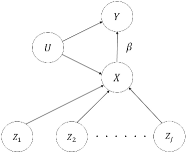
Figure 1: Directed acyclic graph (DAG) representation of the Mendelian randomisation model we consider throughout the paper. The $X\rightarrow Y$ arrow is represented in the model equations by unknown parameter $\beta$.

$$U \sim N(0,0.1),$$ (2.1)

$$X\mid\mathbf{Z},U \sim N\left(\sum\limits_{k=1}^{J}\alpha_{k}Z_{k}+\delta_{X}U,\sigma_{X}^{2}\right),$$ (2.2)

$$\mu =\text{expit}(\omega+\beta X+\delta_{Y}U),$$ (2.3)

$$\rule{0.0pt}{19.91684pt}Y \sim\text{Bernoulli}(\mu),$$ (2.4)

where the symbol $\sim$ stands for “is distributed as” and $\text{expit}(a)\equiv\frac{e^{a}}{1+e^{a}}$. The symbol $N(a,b)$ denotes normal distribution with mean $a$ and variance $b$, and $\sigma_{X}$ is the standard deviation of an independent random perturbation of $X$. Of inferential interest is the causal effect of the exposure $X$ on the outcome $Y$, as quantified by parameter $\beta$, with $\beta=0$ corresponding to absence of the causal effect. The vector parameter $\bm{\alpha}=(\alpha_{1},\alpha_{2},\ldots,\alpha_{J})$ represents the strengths of the pairwise associations between instruments and exposure. This model is adapted from Berzuini et al. (2018) and Zou et al. (2020).

As is common in statistics, the DAG can be interpreted as a way of coding conditional independence relationships that are implicit in the model equations. These relationships are conveniently expressed by using the conditional independence notation of Dawid (1979), where $A\mbox{$\,\perp\!\!\!\perp\,$}B\mid C$ reads: “$A$ is independent of $B$, given $C$”, asserting that the conditional distribution of the random variable $A$, given the value of the random variable $C$, does not further depend on $B$. Note that $A$ is marginal independent of $B$ when $C$ is empty, denoted as $A\mbox{$\,\perp\!\!\!\perp\,$}B$. Our model equations and Figure 1 are consistent with the following two conditions:

1. $\mathbf{Z}\mbox{$\,\perp\!\!\!\perp\,$}U$: confounder independence

2. $Y\mbox{$\,\perp\!\!\!\perp\,$}\mathbf{Z}\mid(X,U)$: exclusion-restriction.

Condition 1 states that each of the instrumental variables included in $\mathbf{Z}$ is independent of $U$. This condition is untestable, due to the fact that $U$ is unobserved.

Condition 2 states that there is no association between $\mathbf{Z}$ and $Y$ other than that mediated by $X$, and can be at best only partially tested. An additional condition is that association between each IV in $\mathbf{Z}$ and $X$ is not null.

Prior specifications required to complete the Bayesian formulation of the model were discussed at length in Berzuini et al. (2018). In our simulations, we have taken $\sigma_{X}$ to follow a priori an inverse-gamma distribution, $\sigma_{X}\sim$ Inv-Gamma(3, 2), and each component of $\bm{\alpha}$ to be independently normally distributed with mean 0.5 and standard deviation 0.2:

$$\bm{\alpha}=\left(\begin{array}[]{c}\alpha_{1}\\ \alpha_{2}\\ \vdots\\ \alpha_{J}\\ \end{array}\right)\sim N\left[\left(\begin{array}[]{c}0.5\\ 0.5\\ \vdots\\ 0.5\\ \end{array}\right),\left(\begin{array}[]{cccc}{0.2}^{2}&0&\cdots&0\\ 0&{0.2}^{2}&\cdots&0\\ \vdots&\vdots&\ddots&\vdots\\ 0&0&\cdots&{0.2}^{2}\\ \end{array}\right)\right].$$

The prior for $\beta$ will be discussed later in this paper.

2.2 Region of Practical Equivalence (ROPE)

Having specified the model equations (2.1-2.4), one would often let the null causal hypothesis (asserting that the causal effect is non-existent) be defined by $\beta=0$. This choice raises a problem: the subspace of data generating processes corresponding to a “non-existent” causal effect is singular with respect to the full space of data generating processes defined by the model, so that, for a continuous prior for $\beta$, the posterior probability of a nonexistent causal effect is zero. From a practical point of view, when inference computations are performed via Markov chain Monte Carlo (MCMC) simulation (Metropolis et al. (1953)) with a continuous prior on $\beta$, the probability of the chain visiting the point-space $\beta=0$ is zero, which prevents us from calculating and comparing posterior probabilities for the “non-existence” and for “existence” hypotheses. This explains why Bayesians resort to Bayes factors. The reason is that Bayes factors avoid the problem by comparing marginal likelihoods, albeit incurring other practical and conceptual difficulties. A popular (albeit risky) option is to treat Bayesian posterior credible intervals as if they were classical confidence intervals, that is, by deciding in favour of the null (non existence) if and only if the credible interval covers the value 0. This option leads to generally incorrect inferences, thereby acting against scientific reproducibility (and against a fair comparison of Bayesian vs classical methods).

We avoid the singularity problem by defining “non existence” of the causal effect as corresponding to the value of $\beta$ falling within a neighborhood around $\beta=0$, called the region of practical equivalence (Kruschke (2018)), or the region of practical importance, hereafter referred to as ROPE. This enables us to calculate a posterior probability over the “non-existence” subspace, as a basis for the hypothesis test decision. We shall claim a “discovery” when the posterior probability of $\beta$ falling in the ROPE does not exceed a specified threshold. For a user-specified real positive $T$, the non-existence (of the causal effect) and existence hypotheses, $H_{0}$ and $H_{1}$, respectively, are defined as follows:

$$H_{0}:-T\leq\beta\leq T,$$

$$H_{1}:\beta\notin[-T,T],$$

with the user-specified $[-T,T]$ interval, which we have taken without loss of generality to be symmetric with respect to zero, acting as ROPE.

The value of $T$ should in principle be chosen in such a way that ROPE contains values of $\beta$ that have small enough absolute magnitudes to be devoid of practical relevance (Kruschke (2018)). Later in this paper we calibrate $T$ with respect to the data and to the model prior distribution. Moreover, use of an interval null hypothesis attenuates problems due to the model being (as all models) wrong, a consequence of this being sufficient amount of data will always cause the point null hypothesis to be rejected in favour of effects of negligible magnitude. The ROPE approach regards effects of small magnitude as practically “equivalent to zero”.

2.3 Causal discovery decision rule based on ROPE posterior odds

Generally speaking, once the model has been specified, we would run one or more Hamiltonian MCMC chains (see Betancourt (2017)) in the space of the unknown model parameters, and then focus on the posterior samples for a particular (typically scalar) parameter that informs us about the causal effect. One possibility is to consider the sampled values of parameter $\beta$ in Equations (2.3-2.4). Precisely, we would consider the proportion $V_{1}$ of sampled values of $\beta$ falling outside the ROPE, and the proportion $V_{0}$ of values falling inside the ROPE. The ratio of thecsevtwo quantities provides a simulation consistent approximation to the posterior odds of $\beta$ falling inside the ROPE, and an input to the following ternary Causal Discovery Decision Rule (CDDR) (Schönbrodt and Wagenmakers (2018)):

• If $\frac{V_{0}}{V_{1}}>10$, accept the non-existence hypothesis with confidence;

• If $\frac{V_{0}}{V_{1}}<0.1$, accept the existence hypothesis (and claim a causal discovery) with confidence;

• If $0.1\leq\frac{V_{0}}{V_{1}}\leq 10$, conclude in favour of an uncertain evidence of a causal effect (uncertain outcome of the decision).

Now we discuss the prior distribution for the causal effect magnitude $\beta$. One possibility would be to assign $\beta$ a mixture prior distribution, that puts a $\pi_{0}$ probability on $\beta$ falling in the ROPE, and a complementary, $(1-\pi_{0})$, probability on this parameter being drawn from a locally uninformative continuous distribution that we, without loss of generality, assume to be normal. Whenever we wish to express our prior ignorance about the existence of a causal effect, a reasonable value for $\pi_{0}$ is $0.5$. One way of implementing the above prior within the model would be by expressing the prior distribution of $\beta$ conditional on an unobserved binary indicator which takes value $1$ in case of “existence” of the causal effect, and value $0$ in the case of “non-existence”, so that this indicator would effectively act as a switch between the two components of the mixture prior. A causal discovery decision rule could even be constructed on the basis of such parameter, but we shall henceforth adopt the above CDDR based on the posterior samples of $\beta$. The samples are drawn according to the procedure of the nect subsection.

2.4 Importance sampling calculation of the posterior odds

The posterior samples of $\beta$ can be conveniently generated by using the following mixture prior resampling scheme. Let $\theta$ denote the full set of unknown quantities in the model (including parameters and missing data values) minus the causal effect $\beta$. The idea is to apply MCMC to a model where the “true” (mixture) prior for $\beta$, which we denote as $p^{true}(\beta)$, is replaced by a (computationally more convenient) continuous prior denoted as $p^{used}(\beta)$. A sample $S$ of values of $(\beta,\theta)$ will thus be generated from the “incorrect” posterior distribution

$$\pi^{used}(\beta,\theta\mid D) \propto\;\;p(D\mid\beta,\theta)\;\;p^{used}(\beta,\theta)$$ (2.5)

where the symbol $\propto$ stands for “proportional to” and $D$ denotes the data.

The idea is then to exploit principles of importance sampling in order to correct for the fact that we are sampling (2.5) instead of the correct posterior. This is described in the following.

The true posterior probability for $(\beta,\theta)$ is given, up to a proportionality constant we do not need to compute, by

$$\pi^{true}(\beta,\theta\mid D)\propto p(D\mid\beta,\theta)\;p^{true}(\beta,\theta).$$

By assuming $p^{true}(\beta,\theta)=p^{used}(\beta)p^{true}(\theta)$, the above equation can be re-written as

$$\pi^{true}(\beta,\theta\mid D) \propto p(D\mid\beta,\theta)\;\;p^{used}(\beta,\theta)\;\;\frac{p^{true}(\beta)}{p^{used}(\beta)}$$ (2.6)

$$\propto\pi^{used}(\beta,\theta\mid D)\;\;\;\omega(\beta),$$

where

$$\omega(\beta)\equiv\frac{p^{true}(\beta)}{p^{used}(\beta)}.$$

Let $S$ denote a set of $K$ samples of $(\beta,\theta)$,

$$S\equiv\{\beta^{[k]},\theta^{[k]}\},~{}~{}~{}~{}~{}~{}k=1,\ldots,K,$$

generated from the “incorrect” posterior distribution $\pi^{used}(\beta,\theta\mid D)$. A reweighted resampling of $S$ with replacement, with the weight of each $k$th sample, $\omega^{[k]}$, obtained by evaluating $\omega(\beta)$ at it, $\omega^{[k]}\equiv\omega(\beta^{[k]})$, will yield a set of samples of $(\beta,\theta)$ we can think of as generated from the correct posterior. In particular, it will yield a set of posterior samples for $\beta$ which we can use according to the CDDR of the preceding subsection to determine the test decision outcome.

Recall our definition of a prior for $\beta$ in the form of a mixture of a locally uninformative normal distribution, say $N(0,10^{2})$, and a uniform density over $[-T,T]$. We call this mixture prior “true prior” of $\beta$, denoted by $p^{true}(\beta)$. Consider an alternative model which only differs from the intended model by the fact that it replaces $p^{true}(\beta)$ with a computationally more manageable prior for $\beta$, which we denote as $p^{used}(\beta)$, and, without loss of generality, take to be $N(0,10^{2})$. Then the choice $\pi_{0}=0.5$ leads to

$$\omega^{[k]}=\frac{0.5\cdot N(\beta^{[k]}\mid 0,10^{2})+0.5\cdot Unif(\beta^{[k]}\mid-T,T)}{N(\beta^{[k]}\mid 0,10^{2})}.$$

where $Unif(q\mid-T,T)$ denotes the probability density at a real point $q$ under a rectangular (uniform) distribution with support $(-T,T)$. For a sample $\beta^{[k]}$ falling outside $[-T,T]$ this weight will be $0.5$. For a sample $\beta^{[k]}$ falling inside $[-T,T]$ it will be $0.5+\frac{1}{4\cdot T\cdot N(\beta^{[k]}\mid 0,10^{2})}$. Hence samples falling outside the interval will be downweighted with respect to the samples inside, the downweighting being the more pronounced the smaller the interval.

2.5 Calibration

Hypothesis test decision rules should be evaluated, more precisely calibrated, in accord with the principles of decision-theory, by using some measure of the expected loss. We shall consider ternary decisions with possible outcomes “accept the hypothesis $H_{1}$ of existence of the causal effect”, “accept the hypothesis $H_{0}$ of absence of the causal effect” and “uncertain outcome”. Let $L(\beta,A)$ denote the loss incurred when the true value of the causal parameter is $\beta$ and the chosen decision outcome is $A$. Let this function be defined as

$$L(\beta=0,H_{0}\;\mbox{accepted with confidence})\hskip 28.45274pt = 0,$$

$$L(\beta=0,\mbox{uncertain outcome})\hskip 71.13188pt = a,$$

$$L(\beta=0,H_{1}\;\mbox{accepted with confidence})\hskip 28.45274pt = 1,$$

$$L(\beta=\beta^{*},H_{0}\;\mbox{accepted with confidence})\hskip 22.76228pt = 1,$$

$$L(\beta=\beta^{*},\mbox{uncertain outcome})\hskip 65.44142pt = a,$$

$$L(\beta=\beta^{*},H_{1}\;\mbox{accepted with confidence})\hskip 22.76228pt = 0,$$

where $\beta^{*}\neq 0$.

The choice of $a$, with $0\leq a\leq 1$, will depend on the applicative context. Large values of $a$ will be appropriate if conservative discoveries are desired at the cost of some decisions being held in a limbo.

The next section describes a simulation experiment where we compare results of a frequentist and of a Bayesian MR analysis of the same data, by using different priors. In each of the simulated scenarios, the comparison is based on the expected loss:

$$L \equiv p(\mbox{uncertain outcome}\mid\beta=0)\times{\rm I}_{\beta=0}\times a+$$

$$p(H_{1}\;\mbox{accepted with confidence}\mid\beta=0)\times{\rm I}_{\beta=0}+$$

$$p(H_{0}\;\mbox{accepted with confidence}\mid\beta=\beta^{*})\times{\rm I}_{\beta=\beta^{*}}+$$

$$p(\mbox{uncertain outcome}\mid\beta=\beta^{*})\;{\rm I}_{\beta=\beta^{*}}\;\times a.$$

with the probabilities $p(.\mid\beta=.)$ estimated by simulation. The first and last terms in the expression of $L$ will be zero in the frequentist case. The intention in the experiment will by no means be to prove that one of the two approaches is superior, but rather that use of a Bayesian approach with a ternary decision rule might often be a good idea, and that one reason for this is that the frequentist method (but not the Bayesian one) is generally “handicapped” by its inability to allow for an uncertain outcome.

3 Simulation experiment

We are now going to describe a simulation experiment where the expected loss criterion of the preceding section is used to compare performances of a frequentist and of a Bayesian MR method in realistic data analysis scenarios. By allowing for randomly missing values of the exposure variable, we shall factor into the experiment the ability of the Bayesian approach to coherently handle missing data, as discussed elsewhere (Zou et al. (2020)). No outcome-dependent selection mechanisms were simulated.

3.1 Experiment design

We simulated situations where the following two datasets are jointly analysed:

• Dataset $A$: collected from sample individuals with complete observations for $(\mathbf{Z},X,Y)$;

• Dataset $B$: collected from individuals with completely observed values for $\mathbf{Z}$ and $Y$, and completely missing values of $X$.

We assumed no overlap, i.e., no individuals shared between $A$ and $B$. Let the symbol $D_{1}$ denote the combined dataset $A\cup B$. In the special case where $B$ is empty, dataset $D_{1}$ lends itself to standard one-sample MR analysis. Analysis of $D_{1}$ will otherwise fall in the “one-sample MR with missing $X$-data” category. With reference to Equations (2.1)-(2.4), we considered 18 different configurations:

• the rate of missingness of $X$: (80%, 40%, 0%)

• the strength of the $\bm{\alpha}=(\alpha_{1},\alpha_{2},\ldots,\alpha_{J})$ coefficients, assumed to be the same for all IVs: $(\mathbf{0.3}$, $\mathbf{0.1}$, $\mathbf{0.05})$

• the magnitude of the causal effect $\beta$: (0.3, 0)

In total, we considered $3\times 3\times 2=18$ scenarios were simulated. Throughout the experiment, parameters $\delta_{X}$ and $\delta_{Y}$ were set to 1 and the number $J$ of instruments was set to $15$. Two hundred datasets were simulated under each separate scenario, for a total of 3,600 datasets simulated during the experiment. Each of these 3,600 datasets was generated by the following sequence of steps:

1. simulate 1000 independent individuals characterized by realistic realizations of $\mathbf{Z}$ and then, on the basis of the $Z$s, generate for each individual values of $X$ and $Y$ in accord with Equations (2.1)-(2.4). Call the resulting dataset H;

2. randomly sample $n_{A}$ individuals from H, without replacement, and let the selected individuals, each with a completely observed ($\mathbf{Z},X,Y$) vector, form the dataset that we have previously labelled as $A$;

3. randomly sample $n_{B}$ individuals from $\textbf{H}\setminus A$ and take each of them to be characterized by observed ($\mathbf{Z},Y$), with their corresponding values of $X$ treated as missing. Let these selected individuals form the dataset that we have previously labelled as $B$. At this point, we were ready to apply MR to data $D_{1}=A\bigcup B$.

The sample size of $D_{1}$ was set to be 400 throughout the experiment. Parameter $n_{B}$ was controlled by the rate of missingness of $X$ for the relevant scenario. For example, for a rate of missingness of $X$ of 80%, we had $n_{A}=80$ and $n_{B}=320$. In the special case of a 0% rate of missingness of $X$, it was $D_{1}\equiv A$. MCMC computations were performed with the aid of the probabilistic programming language Stan (Stan Development Team (2014); Wainwright and Jordan (2008)). Missing data imputation and causal effect estimation were performed simultaneously via MCMC, by exploiting the substantial equivalence of unknown model parameters and missing values in Bayesian analysis.

We compared our Bayesian method with the following two frequentist approaches to two-sample MR: two-stage least squares (2SLS) regression (Burgess and Thompson (2014)) in the case of a 0% rate of missingness of $X$, and inverse-variance weighted (IVW) estimation (Bowden et al. (2016)) otherwise. Application of frequentist IVW required the observed values of $Y$ in Dataset $A$ to be discarded to comply with the frequentist two-sample analysis mechanism. After each frequentist MR analysis of a simulated dataset, the null causal hypothesis $H_{0}:\beta=0$ was accepted iff the 95% confidence interval for $\beta$ contained the null value 0. The alternative hypothesis $H_{1}:\beta\neq 0$ was otherwise accepted.

As far as the Bayesian analysis of each simulated dataset is concerned, we used the previously discussed computational procedure and CDDR decision rule to determine the outcome of the test, with the threshold $T$ and parameter $a$ randomly drawn from uniform distributions: $T\sim Unif(10^{-2},10^{-1})$ and $a\sim Unif(0,0.6)$. The information generated by the above procedure allowed us to compute the expected losses for the MR methods under comparison, a high expected loss implying a high rate of false positives/negatives.

3.2 Experiment results

Figure 2 displays the results, when the $\beta=0$, of the frequentist and Bayesian MR for each combination of IV strength and missing rate. The flat grey surface in each panel depicts the loss of the frequentist MR and the coloured surfaces the loss of the Bayesian method. Unsurprisingly, the average loss incurred by the frequentist approach does not appear depend on the values of $T$ or $a$, as these parameters are not involved in the calculation of frequentist loss.

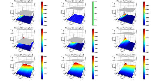
Figure 2: Loss of the frequentist and our Bayesian MR with binary $Y$ when $\beta=0$. Each panel represent each combination of the missing rate of $X$ ($80\%,$ $40\%$ and $0\%$) and the IV strength (0.3, 0.1 and 0.05) based on 200 simulated datasets.

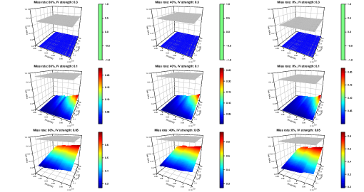
Figure 3: Loss of the frequentist (grey flat surfaces) and our Bayesian MR(coloured curves) with binary $Y$ when $\beta=0.3$. Each panel represent each combination of the missing rate of $X$ ($80\%,$ $40\%$ and $0\%$) and the IV strength (0.3, 0.1 and 0.05) based on 200 simulated datasets.

Our Bayesian method showed a lower loss almost uniformly across the configurations, with the loss decreasing with an increasing IV strength. There were noticeable fluctuations of the loss when $T$ was small. This is because the weight $0.5+\frac{1}{4\cdot T\cdot N(\beta^{[k]}\mid 0,10^{2})}$ decreases as $T$ increases. When there were not enough samples falling in the wider tolerance interval to offset the decrease of weight, the loss became unstable. For example, considering two intervals $[-T_{1},T_{1}]$ and $[-T_{2},T_{2}]$ ($T_{1}<T_{2}$), suppose there are 10 sampless falling in $[-T_{1},T_{1}]$, with weight $0.5+\frac{1}{4\cdot T_{1}\cdot N(\beta^{[k]}\mid 0,10^{2})}$, $k=1,\ldots,10$ (each point has a different density $N(\beta^{[k]}\mid 0,10^{2})$). When $T$ increases from $T_{1}$ to $T_{2}$, the weights will reduce to $0.5+\frac{1}{4\cdot T_{2}\cdot N(\beta^{[k]}\mid 0,10^{2})}$ with the density values unchanged. Thus, if there are not enough new samples falling in $[-T_{2},T_{2}]$ to offset the decrease in weight, the loss will fluctuate.

When $\beta=0.3$, our Bayesian method resulted in no loss when $\bm{\alpha}=\mathbf{0.3}$ (Figure 3), showing a positive impact of higher IV strength on decision-making. This is because no posterior samples fell in $[-T,T]$ for all different values of $T$. As IV strength decreased, the posterior distribution had a larger standard deviation and some samples fell in the interval for a large $T$, and we started to see a loss from the Bayesian method. When $T$ continued to increase, the wider interval contained more samples, leading to a higher loss. When the level of IV strength decreased, the loss increased in our method. However, our method was still consistently better than the frequentist with a lower loss.

4 Is Obesity a strong cause of Juvenile Myocardial Infarction?

With the improvement of living standards, recent decades have witnessed a dramatic increase in prevalence of obesity. A common measure of obesity is the body mass index (BMI), defined as the weight in kilograms divided by the square of the height in meters. A high value of BMI is taken to indicate an excess of body fat. Studies have demonstrated that obesity acts as a major causal risk factor for cardiovascular disease and hypertension. To the best of our knowledge, no studies have examined these links by an analysis that focuses on occurrence of MI at an early age. Yet, early age is where the influence of genetics on cardiovascular events is at its highest, which makes a MR analysis of the causes of early-age MI most appealing and less vulnerable to biases. Motivated by these considerations, our study focuses on the causal effect of BMI on occurrence of a MI before age 45.

Our analysis was based on data from an Italian study of the genetics of infarction (Berzuini et al. (2012)). JMI cases were ascertained on the basis of hospitalization for acute myocardial infarction between ages 40 and 45, from 1996 to 2002. The recorded values of BMI, measured after occurrence of JMI, were considered representative of pre-JMI obesity level.

One caveat in the analysis we are going to describe is that post-JMI BMI levels may reflect recent changes in the patient’s lifestyle and behaviour, resulting in rather weak genetic associations with BMI and, as a consequence, in higher vulnerability to bias.

A graphical representation of the adopted MR model is shown in Figure 4. The narrow age range of the event in our study attenuates problems introduced by censoring, and justifies our choice of representing disease outcome as a binary variable (1: had MI, 0: did not have MI) in our analysis.

The single nucleotide polymorphisms (SNPs) associated with BMI were identified based on the datasets from genome-wide association study (GWAS) and UK Biobank ($P\leq 5\times 10^{-8}$). Through the command-line program Plink (Purcell and Chang (2021)), as many as 360 independent ($r^{2}<0.001$) SNPs were selected and then used as instruments for assessment of obesity causal effect on JMI. SNPs were coded as 3 valued $(0,1,2)$ counts of the minor allele, after appropriate cross-study harmonization. In total, 521 independent individuals were studied in the illustrative analysis based on our Bayesian method. Values of BMI were standardised (mean 0, standard deviation 1) prior to analysis. The observed values of the following 5 potential confounders were included in the model: sex (Male/Female), smoking status (Yes/No) alcohol consumption (Yes/No), cocaine consumption (Yes/No) and age.

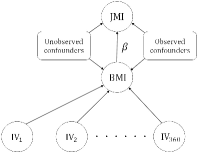
Figure 4: MR model with 360 instrumental variables, ($\rm IV_{1}$, $\rm IV_{2}$, …, $\rm IV_{360}$), used in our illustrative study to assess the causal effect of BMI on juvenile myocardial infarction (JMI). Observed values of 5 potential confounders (sex, smoking status, alcohol consumption, cocaine consumption and age), were included in the model (see main text). The model assumes there are no associations between IVs and JMI other than those mediated by BMI.

We ran the Markov chain in the space of the model unknowns (model parameters and missing BMI values). The chain was 20,000 iterations long, the last 5,000 iterations being used for purposes of inference. Figure 5 shows superimposed posterior density plot (Panel (a)) and Bayesian posterior parameter trace plot (Panel (b)) for the causal effect of standardized BMI on JMI. The trace in (b) indicates reasonably good mixing of the chain, with $\widehat{R}=1.002$. For each of the thresholds $(0.02,0.04,0.06,0.08)$ for $T$, after the mixture prior resampling discussed in Section 2.4, we had $0.1<\frac{V_{0}}{V_{1}}<10$. In the light of this, and in spite of the 95% credible interval for $\beta$ lying entirely in the positive real axis, our test decision was uncertain evidence in favour of a causal effect of genetically induced changes in obesity on JMI.

(a) Posterior distribution curve for $\beta$.

(b) Bayesian posterior parameter trace plot for $\beta$.

Figure 5: Estimated causal effect of standardized BMI on JMI, based on the Bayesian Mendelian randomization analysis we have performed data from our illustrative study. $(a)$ Posterior distribution curve for causal parameter $\beta$ with posterior mean 0.303 and 95% credible interval (0.069, 0.550). $(b)$ Bayesian posterior parameter trace plot for $\beta$.

5 Discussion

In our approach to Bayesian MR analysis, the hypothesis $H_{0}$ of non-existence of the causal effect of interest is represented by a user-specified interval of values of the causal effect, which we may refer to by using the established term "region of practical equivalence" (ROPE). Importance sampling technology is used to approximate the posterior odds of the causal effect falling inside this interval. A sufficiently large value of this posterior odds will lead to acceptance of the null no-effect hypothesis, whereas a sufficiently small value will lead to acceptance of the alternative hypothesis, and to a causal discovery claim. A third, “uncertain”, decision outcome is available for situations where the posterior odds is neither large nor small enough, indicating scarce data support to either hypothesis. The uncertain outcome has been introduced to reduce chances of placing undue confidence in a hypothesis that is only weakly supported from the data . We have incorporated this ternary test decision logic into the Bayesian MR framework proposed by Berzuini et al. (2018) and further refined by Zou et al. (2020). The decision rule can be calibrated via simulation by acting on the differential weighting parameters of a loss function.

In a simulation experiment, we have compared our method with a standard MR method in terms of expected loss, by allowing loss function parameters to vary within reasonably wide intervals. The experiment suggests that, within the examined scenarios, our method outperforms standard MR, and this may be due to the latter being handicapped by inability to accommodate decision uncertainty. We consider our proposed method as a contribution to research on more reproducible MR analysis.

We have applied our proposed method to a MR study of the causal effect of obesity on juvenile myocardial infarction, based on a unique dataset. The study concludes in favour of an uncertain evidence of a non-null causal effect.

Acknowledgments

We thank Philip Dawid for advice on methodological aspects of the work, and Luisa Bernardinelli and Diego Ardissino for providing the data for the Illustrative Study and contributing to the interpretation of the results. Any misinterpretation is, of course, entirely a responsibility of the authors.

Declarations

Funding This work was funded by Manchester-CSC. The funder had no role in study design, data generation and statistical analysis, interpretation of data or preparation of the manuscript.

Competing interests The authors declare that they have no competing interests.

Ethics approval Not applicable

Consent to participate Not applicable

Consent for publication Not applicable

Availability of data and materials The data of simulation experiment and illustrative study is available from the corresponding author upon request.

Code availability The code of data simulations and illustrative study is available from the corresponding author upon request.

Authors’ contributions CB conceived the study. CB and HG supervised the study. LZ performed simulations and statistical analysis. TF conceived the illustrative study and provided the data. LZ, CB and HG interpreted statistical results and wrote the manuscript. LZ, TF, CB and HG read and approved the final manuscript.

References

- Kruschke (2018) John K. Kruschke. Rejecting or accepting parameter values in bayesian estimation, 2018. http://journals.sagepub.com/doi/10.1177/2515245918771304.
- Katan (1986) Martjin B Katan. Apolipoprotein E isoforms, serum cholesterol, and cancer. The Lancet, 327:507–508, 1986.
- Smith and Ebrahim (2003) George Davey Smith and Shah Ebrahim. Mendelian randomization: can genetic epidemiology contribute to understanding environmental determinants of disease? International Journal of Epidemiology, 32:1–22, 2003.
- Lawlor et al. (2008) Debbie A. Lawlor, Roger M. Harbord, Jonathan A. C. Sterne, Nic Timpson, and George Davey Smith. Mendelian randomization: Using genes as instruments for making causal inferences in epidemiology. International Journal of Epidemiology, 27:1133–1163, 2008.
- Jeffrey (2009) Wooldridge Jeffrey. Instrumental variables estimation and two stage least squares. Introductory Econometrics: A Modern Approach. Nashville, TN: South-Western, 2009.
- Berger and Sellke (1987) James O. Berger and Thomas Sellke. Testing a Point Null Hypothesis: The Irreconcilability of P Values and Evidence. Journal of the American Statistical Association, 82:112–122, 1987.
- Stanton (2020) Jeffrey M. Stanton. Evaluating Equivalence and Confirming the Null in the Organizational Sciences. The American Statistician, 24(3):491–512, 2020.
- (8) Riko Kelter. A New Bayesian Two-Sample t Test and Solution to the Behrens-Fisher Problem Based on Gaussian Mixture Modelling with Known Allocations. Statistics in Biosciences, 2021. https://doi.org/10.1007/s12561-021-09326-2.
- Kelter (2021) Riko Kelter. Bayesian Hodges-Lehmann tests for statistical equivalence in the two-sample setting: Power analysis, type I error rates and equivalence boundary selection in biomedical research. BMC Medical Research Methodology, 21(171), 2021.
- Liao et al. (2021) J. G. Liao, Vishal Midya, and Arthur Berg. Connecting and Contrasting the Bayes Factor and a Modified ROPE Procedure for Testing Interval Null Hypotheses. The American Statistician, 75(3):256–264, 2021.
- Maximilian et al. (2021) Linde Maximilian, Tendeiro Jorge N., Selker Ravi, Wagenmakers Eric-Jan, and van Ravenzwaaij Don. Decisions about equivalence: A comparison of TOST, HDI-ROPE, and the Bayes factor. Psychological Methods, 2021.
- Stevens and Hagar (2022) Nathaniel T. Stevens and Luke Hagar. Comparative Probability Metrics: Using Posterior Probabilities to Account for Practical Equivalence in A/B tests. The American Statistician, 2022.
- Berzuini et al. (2018) Carlo Berzuini, Hui Guo, Stephen Burgess, and Luisa Bernardinelli. A Bayesian approach to Mendelian randomization with multiple pleiotropic variants. Biostatistics, 21(1):86–101, 2018.
- Zou et al. (2020) Linyi Zou, Hui Guo, and Carlo Berzuini. Overlapping-sample Mendelian randomisation with multiple exposures: a Bayesian approach. BMC Medical Research Methodology, 20:295, 2020.
- Dawid (1979) A. P. Dawid. Conditional independence in statistical theory. Journal of the Royal Statistical Society: Series B (Methodological), 41(1):1–15, 1979.
- Metropolis et al. (1953) Nicholas Metropolis, Arianna W. Rosenbluth, Marshall N. Rosenbluth, Augusta H. Teller, and Edward Teller. Equation of State Calculations by Fast Computing Machines. Journal of Chemical Physics, 21:1087–1092, 1953.
- Betancourt (2017) Michael Betancourt. A Conceptual Introduction to Hamiltonian Monte Carlo, 2017. https://arxiv.org/pdf/1701.02434.
- Schönbrodt and Wagenmakers (2018) Felix D. Schönbrodt and Eric-Jan Wagenmakers. Bayes factor design analysis: Planning for compelling evidence. Psychonomic Bulletin & Review, 25:128–142, 2018.
- Stan Development Team (2014) Stan Development Team. STAN: A C++ library for probability and sampling, version 2.2. http://mc-stan.org/, 2014.
- Wainwright and Jordan (2008) Martin J. Wainwright and Michael I. Jordan. Graphical Models, Exponential Families, and Variational Inference. Foundations and Trends in Machine Learning, 1:1–305, 2008.
- Burgess and Thompson (2014) Stephen Burgess and Simon G. Thompson. MENDELIAN RANDOMIZATION Methods for Using Genetic Variants in Causal Estimation. CRC Press, 2014.
- Bowden et al. (2016) Jack Bowden, George Davey Smith, Philip C. Haycock, and Stephen Burgess. Consistent Estimation in Mendelian Randomization with Some Invalid Instruments Using a Weighted Median Estimator. Genetic Epidemiology, 40:304–314, 2016.
- Berzuini et al. (2012) Carlo Berzuini, Stijn Vansteelandt, Luisa Foco, Roberta Pastorino, , and Luisa Bernardinelli. Direct Genetic Effects and Their Estimation From Matched Case-Control Data. Genetic Epidemiology, 36(6):652–662, 2012.
- Purcell and Chang (2021) Shaun Purcell and Christopher Chang. PLINK 1.9. www.cog-genomics.org/plink/1.9/, 2021.