Displaced Searches for Light Vector Bosons at Belle II

Abstract

With a design luminosity of 50 ab^-1 and detectors with tracking capabilities extending beyond 1 m, the Belle II experiment is the perfect laboratory for the search of particles that couple weakly to the Standard Model and have a characteristic decay length of a few centimetres and more. We show that for models of dark photons and other light vector bosons, Belle II will be successful in probing regions of parameter space which are as of now unexplored by any experiment. In addition, for models where the vector boson couples sub-dominantly to the electron and quarks as compared to muons, e.g. in the $L_{\mu}-L_{\tau}$ model, Belle II will probe regions of mass and couplings compatible with the anomalous magnetic moment of muon. We discuss these results and derive the projected sensitivity of Belle II for a handful of other models. Finally, even with the currently accumulated data, $\sim 200$ fb^-1, Belle II should be able to cover regions of parameter space pertaining to the X(17) boson postulated to solve the ATOMKI anomaly.

1 Introduction

The physics of weakly coupled light particles has gained a lot of traction in recent times. This is motivated in equal parts by the interest in weakly interacting dark sectors, the persistence of different anomalies at low energies, and the establishment of dedicated experimental programs designed to look for signatures of new light degrees of freedom. One such example is the Belle II Belle-II:2018jsg experiment that has recently started to collect data from the collision of $e^{+}e^{-}$ beams provided by the SuperKEKB collider Akai:2018mbz . The Belle II experiment, like its predecessors, the BaBar BaBar:1998yfb and the Belle Belle:2012iwr experiments, is expected to push the high intensity frontier of particle physics to new limits. Light ($\sim$ 1 GeV) new physics can produce a plethora of striking signatures at the Belle II experiment, of which, in this paper, we concentrate on tracks that can be reconstructed to coincide at vertices away from the interaction point (IP), i.e., displaced vertices. There has been a lot of attention in recent times on displaced vertex searches at the intensity frontier. For example, strong projected limits are obtained in the context of Belle II for sterile neutrinos Dib:2019tuj , heavy QCD axions Bertholet:2021hjl based on the two loop amplitude computed in Ref. Chakraborty:2021wda , and dark photons (DP) Duerr:2019dmv ; Ferber:2022ewf . For lighter DP masses, strong constraints have been obtained Galon:2022xcl using displaced DP searches at the MUonE experiment Abbiendi:2022oks , recently.

From a theoretical perspective, light vector bosons are motivated by many new physics (NP) scenarios. Arguably, the most popular of these models are those where the light vector boson acts as a portal between the Standard Model (SM) particles and some new dark sector Boehm:2003hm ; Fayet:2004bw . The DP model is the most well studied example of such portals to dark sectors. In these models, only dark sector particles have couplings to the new vector boson, the DP ($A^{\prime}$). The $A^{\prime}$ field strength has kinetic mixing with the SM photon Okun:1982xi ; Galison:1983pa ; Holdom:1985ag which induces interactions between the $A^{\prime}$ and the SM fermions. Another class of models of interest are those where the anomaly free global symmetries of the SM are gauged, viz., $L_{\mu}-L_{\tau}$, $L_{e}-L_{\mu}$, $L_{e}-L_{\tau}$, and $B-L$ Fayet:1980rr ; Foot:1990mn ; He:1990pn ; He:1991qd . Here, $L_{i}$ is the lepton number corresponding to the $i$ type lepton, $B$ and $L$ are the flavor-blind baryon number and lepton number respectively. Also, $L_{i}-L_{j}$/$B-L$ can act as portals to dark sectors that carry lepton number and/or baryon number Kadastik:2009cu ; Frigerio:2009wf ; Heeck:2015qra ; Bandyopadhyay:2017uwc ; Foldenauer:2018zrz .

Light vector bosons, especially the $L_{\mu}-L_{i}$ type vectors, have recently gained a lot of attention in the context of the muon and the electron $g-2$ anomalies Ma:2001md ; Pospelov:2008zw ; Heeck:2011wj ; Buras:2021btx . The $(g-2)_{\mu}$ anomaly has persisted across different experiments for about a couple of decades Muong-2:2006rrc ; Aoyama:2020ynm , with a new measurement quoting a tension of 4.2$\sigma$ between the SM and the experimental numbers Muong-2:2021ojo . Although, a recent lattice result questions the validity of this discrepancy Borsanyi:2020mff , the anomaly holds as of now and the experimental precision is expected to be improved at upcoming facilities at the Fermilab Muong-2:2015xgu and J-PARC Abe:2019thb . Although the muon anomaly is more striking, there also exists an anomaly for the electron magnetic moment. The status of this anomaly is intriguing as two different computations with the fine-structure constant ($\alpha_{\mathrm{EM}}$) measured from two different sources, the Caesium (Cs) Parker:2018vye ; Aoyama:2017uqe and Rubidium (Rb) Davoudiasl:2018fbb ; Morel:2020dww atoms, give results on either side of the SM value.

Given the theoretical interest in these particles, there have been numerous experimental searches for them. The non-observance of such particles has translated to constraints in the mass–coupling parameter space. To put our work in context, we briefly discuss the relevant experiments which have already given constraints using visible and invisible channels. To probe visible channels, one requires $M_{A^{\prime}}>1$ MeV ($>2m_{e}$). The visible channels can be further classified into prompt and displaced, i.e., cases where the vector boson decays immediately after production and cases where it propagates for a finite distance before decaying. For a particle to decay away from the interaction point, it needs to have comparatively small decay widths. Hence, displaced vertex searches typically bound regions of small couplings and masses compared to prompt searches. We now categorize the existing experimental searches for an $A^{\prime}$-like boson at different experimental setups:

1. Searches in $e^{+}e^{-}$ Colliders: In lepton colliders, the most prominent production mode for the $A^{\prime}$ is the $t$-channel annihilation of electron positron pairs, $e^{+}e^{-}\to A^{\prime}\gamma$ Fayet:2007ua , followed by the decay of the $A^{\prime}$ to a pair of leptons/hadrons. The background is mostly dominated by the irreducible $s$-channel process $e^{+}e^{-}\to\ell^{+}\ell^{-}\gamma$. So far, the most stringent bounds on the parameter space from $e^{+}e^{-}$ collisions come from the BaBar experiment BaBar:2014zli ; BaBar:2016sci ; BaBar:2017tiz . The projected limits from Belle II Belle-II:2018jsg ; Jho:2019cxq are supposed to improve this bound a few times. For both these experiments, the center of mass (CoM) energy is around $10$ GeV. On the other hand, the KLOE experiment Anastasi:2015qla ; KLOE-2:2018kqf , operating at the $\phi$ meson resonance ($\sim 1$ GeV) with $2.5$ fb^-1 data, probes significant areas in the low mass region. There are bounds on the $A^{\prime}$ parameter space from the data collected by the BESIII detector, at the BEPCII collider, as well BESIII:2017fwv . We do not show these bounds in our results as the BaBar bounds for the same masses are stronger.

2. Searches at Hadron Colliders: In hadron colliders, the main production mode for light DPs with $M_{A^{\prime}}\lesssim 0.5$ GeV is from meson decays, e.g., $\pi^{0}\to A^{\prime}\gamma$ $\left(\eta\to A^{\prime}\gamma\right)$ etc. For $0.5~{}\text{GeV}<M_{A}^{\prime}<1~{}\text{GeV}$, mixings with the $\rho$, $\omega$, and $\phi$ mesons become important. Whereas, the Drell-Yan process with $q\bar{q}\to A^{\prime}$ gradually takes over for heavier masses. Till date, the strongest bounds from hadron colliders come from the LHCb collaboration, from both prompt and displaced searches LHCb:2017trq ; LHCb:2019vmc . The dominant background for the prompt channel comes from irreducible SM Drell-Yan processes. On the other hand, the largest contribution for displaced searches stem from photon conversions. Rejecting dilepton vertices from the primary vertex can significantly reduce the background to a negligible amount LHCb:2019vmc .

3. Searches at Meson factories: Dedicated experiments like NA48/2 NA482:2015wmo , NA62 NA62:2019meo etc. looked for $\pi^{0}\to A^{\prime}\gamma$ followed by the prompt decay of the DP to lepton pairs. The source of neutral pions are from Kaon decays. These experiments provide the strongest bounds in the light $M_{A^{\prime}}$ region. We only show the bounds from the NA48/2 experiment, as it is stronger than those from NA62.

4. Searches in Proton Beam Dumps: Proton beam dump experiments like CHARM CHARM:1985anb ; Tsai:2019buq , NOMAD NOMAD:1998pxi ; Gninenko:2011uv etc. had a proton beam colliding against a fixed target (Cu and Be respectively). The hit at the target by the proton beam generates a plethora of mesons which subsequently decay to $\gamma A^{\prime}$, $\pi^{0}\to A^{\prime}\gamma$, $\eta^{\prime}\to A^{\prime}\gamma$ etc. The strongest bound, however, comes from the $\nu$-calorimeter I (NuCal) experiment that looks at data from proton beam collisions on Iron at the IHEP-JNR neutrino detector Blumlein:1990ay ; Blumlein:1991xh ; Tsai:2019buq .

5. Searches in Electron Beam Dumps: We look at the following electron beam dump experiments: E137 Bjorken:1988as , E141 Riordan:1987aw ,KEK Konaka:1986cb , Orsay Davier:1989wz , APEX APEX:2011dww , and A1 at MAMI Merkel:2014avp . These experiments exploit the bremsstrahlung process $eZ\to eZA^{\prime}$, where $Z$ is the SM neutral vector boson. The DPs are primarily produced in the forward region with subsequent decays to boosted leptons in the same direction. These experiments use a shielding to absorb SM particles located after their beam dump targets. The dimensions of the shielding restricts the $A^{\prime}$ flight of distance in the lab frame, which in turn sets a limit on the mass-coupling parameter space. For the models where the $A^{\prime}$ does not couple to hadrons, the E137 bound is the strongest among the beam dump bounds. The E141 bound and the Orsay bound also covers complementary regions of the parameter space. Similarly, limits from NA64 NA64:2019auh probe the region in-between the NA48 and the NuCal/E137 bounds.

We emphasise, the NA64 fixed target bound comes from a search of the hypothetical X(17) vector boson. This particle has been proposed as a solution to the $\sim$ 17 MeV ATOMKI anomaly Feng:2016ysn . Multiple experiments at the Tandetron accelerator of ATOMKI have reported anomalies in the angular correlation spectra of $e^{+}e^{-}$ pairs in the decays of both excited$~{}^{8}$Be and$~{}^{4}$He Krasznahorkay:2018snd ; Krasznahorkay:2021joi . As a result of this, different experiments across the globe have dedicated analyses to look for this particle, including NA64. We show later that Belle II displace searches should be sensitive enough to be competitive with the NA64 bound at current luminosities.

In our case, the exclusion limits that we draw entirely depend on displaced signatures of $A^{\prime}$-like vector bosons. To be specific, we look at displaced vertex signatures accompanied by a monophoton. For the decay of the $A^{\prime}$, we look at dilepton ($e+\mu$) final states only. We checked for hadronic final states but did not find any sensitivity of the detector to displaced vertices for the mass ranges where the hadronic (or $\tau$) final states become kinematically accessible. We draw projected limits for two different luminosities. These are the Belle II design luminosity of 50 ab^-1 and a luminosity approximately equal to the amount of data the collaboration is expected to have collected, $\sim$ 200 fb^-1. We find that at the design luminosity, the experiment should be able to bound a large portion of the DP parameter space in a region that is as of now not excluded by any experiment. The region, that Belle II is expected to constrain, falls between the limits from prompt searches at BaBar and NA48/2 on the one hand and those from displaced searches at NuCal, E137 etc. on the other. We also find that even at current luminosities, the limits would be competitive with experiments like NA64 and E141, which aim to bound similar parameter regions as Belle II.

The paper is organised as follows: In Section 2, we discuss the tracking capabilities of the Belle II detector and also discuss in detail our estimates for the displaced vertex reconstruction efficiencies at the trackers. In Section 3, we discuss the relevant theoretical calculations and go on to use the DP model to establish our methodology in obtaining the projected limits. In Section 4, we extend our analysis to some other models of $Z^{\prime}$ vector bosons. The models we discuss are the $L_{i}-L_{j}$, $B-L$ and the protophobic model Fayet:1986rh . Finally, in Section 5, we conclude.

2 Track reconstruction at Belle II

The Belle II experiment collects data from the events generated by the collisions of the SuperKEKB $e^{+}e^{-}$ beams Akai:2018mbz , with asymmetric energies of $E_{+}\simeq 4$ GeV and $E_{-}\simeq 7$ GeV respectively, giving a CoM energy of $\sqrt{s}\simeq 10.6$ GeV. The Belle II detector complex consists of several sub-systems placed in a cylindrical structure around the beam line. For this work, we are entirely interested in the detectors with tracking capabilities. These are, in order of increasing radial distance from the beam line, a silicon-pixel detector (PXD), a silicon-strip detector (SVD) (together called the vertex detector (VXD)), and a central drift chamber (CDC) Belle-II:2018jsg .

Our goal in this paper is to limit the parameter space of light $A^{\prime}$-like bosons, that couple very weakly to the SM. Specifically, we are interested in the regions of parameter space for which such a boson will travel for some distance before decaying to its daughter particles within the detector. A particle produced at the IP and coming out at an angle $\vartheta$, wrt the electron beam, that decays after travelling a distance $l$, will travel $r=l\sin\vartheta$ in the radial direction, measured perpendicular to the beam-line, and $z=l\cos\vartheta$ measured along the direction of the beam-line. If this decay happens within the fiducial volume of interest then the event is accepted with some efficiency, and rejected otherwise. The fiducial volume is defined not only by the physical dimensions of the tracking detectors but also by the requirements of efficient track reconstruction of the decay products of the $A^{\prime}$ inside said volume. As for the dimensions of the relevant components of the detector, the VXD spans a radial distance of 14 mm – 14 cm, while the CDC spans from the end of the VXD to about 1.13 m. Both the VXD and the CDC have a $\theta$ coverage of:

$$17^{\circ}<\theta<150^{\circ}\,,$$ (1)

which we incorporate as angular cuts in our analysis. Also, following Ref. Dib:2019tuj , we impose the following cuts on $r$, $z$:

$$10\;\mathrm{cm}<r<80\;\mathrm{cm}\,;\quad-40\;\mathrm{cm}<z<120\;\mathrm{cm}.$$ (2)

We take $r_{\mathrm{min}}$ = 10 cm to reject backgrounds arising from prompt tracks, e.g., decay products of $K^{0}_{S}$ and $\Lambda$, and tracks originating from secondary interactions of particles with the detector material. The upper limit, $r_{\mathrm{max}}$ = 80 cm ensures that the decay happens deep enough inside the CDC for the resulting tracks to be reconstructed, with the CDC extending till 113 cm. In this paper, we work in the CoM frame, therefore, we scale all axial lengths by the appropriate boost factor, $\gamma=1.04$, between the lab frame and the CoM frame. Belle II has a dedicated algorithm for the reconstruction of vertices away from the collision point, the $V_{0}$-like particle reconstruction algorithm. The efficiency of this algorithm, as demonstrated in Ref. Belle-II:2018jsg , falls with falling $p_{T}$ of the $A^{\prime}$. To incorporate this in our analysis, we impose a conservative $p_{T}$ cut:

$$p_{T}>0.9\;\mathrm{GeV},$$ (3)

which can be relaxed with increase in the efficiency of $V_{0}$ reconstruction.

For a decay vertex that falls within the fiducial volume, there is an efficiency of reconstruction of the tracks of the daughter particles. This reconstruction is performed using track-fitting and track-finding algorithms Belle-II:2018jsg . A complete experimental analysis that employs these tools is beyond the scope of this work. Instead, to estimate the falling efficiency of vertex reconstruction with increasing radial distance from the beam-line, we use the linearly falling function of radial distance ($r$) that has been used in the analysis of Ref. Bertholet:2021hjl :

$$\mathcal{E}(r) =\frac{r_{\mathrm{max}}-r}{r_{\mathrm{max}}-r_{\mathrm{min}}},$$ (4)

where $r_{\mathrm{min/max}}$ have been defined in Eq. 2.

The probability of an $A^{\prime}$, after being produced at the IP of the electron and positron beams, travelling a distance $l$ from the IP before decaying is given by the exponentially falling decay distribution:

$$P(l) =\frac{e^{-l/\lambda}}{\lambda}.$$ (5)

The characteristic length $\lambda$ defines this decay distribution and is determined from the mean-life, $\tau$ of the particle and its boost:

$$\lambda =\frac{|\vec{p}\;(M_{A^{\prime}})|}{M_{A^{\prime}}}\;c\tau(M_{A^{\prime}},g^{\prime}),$$ (6)

where, $c$ is the velocity of light in vacuum and $|\vec{p}|$ is the magnitude of the three-momentum of the particle. Therefore, for a particular point in the $(M_{A^{\prime}},\,g^{\prime})$ parameter space, the probability of identification of a displaced vertex, corresponding to an event with an $A^{\prime}$ coming out in the direction $\vartheta$ is a convolution of the efficiency given in Eq. 4 with the decay length distribution in Eq. 5. Then, with $r=l\sin\vartheta$ and $z=l\cos\vartheta$, the vertex reconstruction efficiency (VRE) distribution, as a function of $\vartheta$, is:

$$\begin{split}\mathcal{E}(\vartheta)&=\frac{1}{\mathcal{N}}\frac{1}{r_{\mathrm{max}}-r_{\mathrm{min}}}\int_{l_{\mathrm{min}}}^{l_{\mathrm{max}}}(r_{\mathrm{max}}-l\,s_{\vartheta})\;e^{-l/\lambda}\;\overline{\Theta}(l)\;dl\,,\\ \mathrm{where}&\quad\overline{\Theta}(l)=\Theta\left(l\,s_{\vartheta}-r_{\mathrm{min}}\right)\,\Theta(r_{\mathrm{max}}-l\,s_{\vartheta})\,\Theta(l\,c_{\vartheta}-z_{\mathrm{min}})\,\Theta(z_{\mathrm{max}}-l\,c_{\vartheta})\;,\\ \mathrm{and}&\quad l_{\mathrm{min}}=r_{\mathrm{min}};\;l_{\mathrm{max}}=\sqrt{r_{\mathrm{max}}^{2}+z_{\mathrm{max}}^{2}},\quad\mathcal{N}=\int_{l_{\mathrm{min}}}^{l_{\mathrm{max}}}\;e^{-l/\lambda}\;\overline{\Theta}(l)\;dl.\end{split}$$ (7)

In the above equation, we have used the shorthand notations $s_{\vartheta}\equiv\sin\vartheta$ and $c_{\vartheta}\equiv\cos\vartheta$. The efficiency under consideration is only for reconstruction of displaced tracks. The final signal estimate also includes an overall particle identification efficiency, as mentioned later.

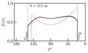
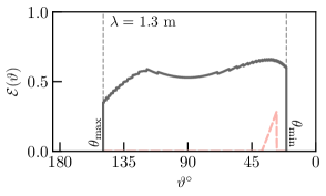
Figure 1: We plot, using solid black lines, the vertex reconstruction efficiency distributions as a function of $\vartheta$ for two different characteristic decay lengths, $\lambda=0.5$ m (left panel) and $\lambda=1.3$ m (right panel). Using red dashed lines, we plot the ‘fake’ efficiency distribution that assumes all the outgoing particles decay at a distance equal to the characteristic decay length of the particle, i.e., assuming a Dirac-delta decay distribution in place of the exponentially falling decay distribution. We also indicate, using dashed lines, the geometric cuts on the angular distribution, as imposed in our analysis.

In an attempt to interpret the VRE distribution in Eq. 7, we plot it for two different values of $\lambda$ in Fig. 1. In both the panels, the solid black line indicates the VRE distribution as obtained from Eq. 7. The dashed red line indicates the efficiency distribution if we had assumed all decays to happen at $\lambda$ only, i.e., if we had used a Dirac-delta distribution, centred at $\lambda$ in place of the exponentially falling distribution. As is intuitively clear from Eq. 7, convoluting the exponential distribution in essence ‘smears’ the distribution that we would have obtained by using a Dirac-delta. Take, for example, an $A^{\prime}$ coming out at $\vartheta=\pi/3$ with $\lambda=1.3$ m, as shown in the right panel of the figure. If the particle decayed at its characteristic length, it would have missed the geometric cuts described above. Hence, the probability of its detection would have been zero. Yet, as its decay is not deterministic, but given from a probability distribution, there is a possibility that it will decay within the fiducial volume, as reflected by the black curve. It is also to be noted that as the decay distribution is exponentially falling, it always peaks at $l=0$. Therefore, particles with a characteristic decay length that is longer than covered in the fiducial volume, have a substantial probability of actually decaying within the said volume.

The VRE distribution gives the probability of detection of a displaced vertex in the direction $\vartheta$ for a particular point in the $M_{A^{\prime}}$ – $g^{\prime}$ space. The probability that an $A^{\prime}$ is produced in the direction $\vartheta$ for a particular point in the $M_{A^{\prime}}$ – $g^{\prime}$ theory space, is given by the differential distribution $d\sigma/d\!\cos\vartheta$. To get the net number of detected events for any given point in the ($M_{A^{\prime}},\,g^{\prime}$) theory space, we need to multiply the $\vartheta$ dependent efficiency with the differential-cross section and integrate. In our computations, we prefer to work with the pseudorapidity,

$$\eta =-\ln\tan\left(\frac{\vartheta}{2}\right),$$ (8)

over $\vartheta$. As the relationship between $\vartheta$ and $\eta$ is one-to-one, it is straightforward to translate the expression for efficiency in Eq. 7 to $\eta$. With that done, the net number of accepted events corresponding to a particular channel, $F$, of decay of the $A^{\prime}$ is given by:

$$N_{\mathrm{Tot}}^{F} =L_{\mathrm{I}}\times\int_{\eta_{\mathrm{min}}}^{\eta_{\mathrm{max}}}d\eta\;\frac{d\sigma}{d\eta}\times\mathrm{BR}_{F}\;\epsilon_{F}\;\mathcal{E}(\eta)\;\Theta\!\left(p_{T}^{\mathrm{min}}-\sin\vartheta(\eta)\,|\vec{p}|\right),$$ (9)

where $N_{\mathrm{Tot}}^{F}$, $L_{\mathrm{I}}$, $\mathrm{BR}_{F}$, and $d\sigma/d_{\eta}$ are the total number of events, the integrated luminosity, the branching ration to $F$, and the differential cross section with respect to the pseudo-rapidity, respectively. The end points of the $\eta$ integral are determined by the geometric cuts given in Eq. 1, which roughly correspond to $-1.3<\eta<1.7$. The factor $\epsilon_{F}$ is the overall efficiency of identification of a final state $F$ at the detector. We exclusively discuss lepton final states in this work, and for the electron and the muon, the efficiencies are:

$$\epsilon_{e} =0.93;\quad\quad\epsilon_{\mu}=0.86.$$ (10)

In Eq. 9, we have also made the $p_{T}$ cut, as given in Eq. 3, explicit. Note that $|\vec{p}|$ is determined by the mass of the particle, from energy conservation:

$$|\vec{p}| =\frac{s-M_{A^{\prime}}^{2}}{2\sqrt{s}}.$$ (11)

In the next section, we use Eq. 9, which contains not only the production cross section and the branching ratio, but also the efficiency distributions and geometric and kinematic cuts, to bound the parameter space of an $A^{\prime}$. We compute the actual cross section of production and the decay widths and branching fractions of the $A^{\prime}$ to do so.

3 Case study: The dark photon

We now use the techniques discussed above in order to constrain the mass–coupling parameter space of the dark photon. We are interested in $e^{+}e^{-}\to\gamma A^{\prime}$, i.e., the $A^{\prime}$ is produced along with a photon in the $t$-channel annihilation of electron positron pairs. The relevant interaction Lagrangian is:

$$\mathcal{L} =g^{\prime}A^{\prime}_{\mu}\bar{f}\gamma^{\mu}(g_{v}^{e}-g_{a}^{e}\gamma_{5})f\,,$$ (12)

where $A^{\prime}$ is a generic neutral vector boson that has both vectorial, $g_{v}^{e}$, and axial, $g_{a}^{e}$, couplings to the electrons ($f)$. The $A^{\prime}$ couples vectorially for all the cases we study, therefore, we drop the $g_{a}^{f}$ in all computations, to avoid confusion. The relevant diagrams for this process are given in Fig. 2.

Figure 2: Diagrams contributing to the process under consideration.

The corresponding spin-summed (averaged) amplitude-squared is:

$$\overline{|\mathcal{A}|^{2}} =8\pi\,\alpha_{\mathrm{EM}}\;{g^{\prime}}^{2}{(g_{v}^{e})}^{2}\,\frac{(s+t)^{2}+(s+u)^{2}}{ut}\,.$$ (13)

Here, $s,t,u$, and $\alpha_{\mathrm{EM}}$ have their usual meanings. Given this amplitude-squared, the differential cross section for the process, in the CoM frame and in the limit of negligible electron mass, is:

$$\frac{d\sigma}{d\eta} =\frac{\alpha_{\mathrm{EM}}}{2s}{g^{\prime}}^{2}({g_{v}^{e}})^{2}\;\frac{\cos^{2}\vartheta(\eta)(s-M_{A^{\prime}}^{2})^{2}+(s+M_{A^{\prime}}^{2})^{2}}{s(s-M_{A^{\prime}}^{2})}.$$ (14)

It is this expression that we plug into Eq. 9 to compute the number of events for a particular $M_{A^{\prime}},\,g^{\prime}$ pair. The form of the differential cross section is the same for all models we discuss, only the parameter $g_{v}^{e}$ is model specific.

We also need the information about the total and partial decay widths of the $A^{\prime}$ in order to calculate the characteristic decay length and also to compute the branching ratios to different final states. The partial width to different channels for $M_{A^{\prime}}\gtrsim\Lambda_{\mathrm{QCD}}$ is straightforward to compute using the effective Lagrangian given in Eq. 12:

$$\Gamma_{A^{\prime}\to f\bar{f}} =\frac{n_{c}^{f}}{12\pi}{g^{\prime}}^{2}{(g_{v}^{f})}^{2}M_{A^{\prime}}\sqrt{1-4\frac{m_{f}^{2}}{M_{A^{\prime}}^{2}}}\;\left(1+2\frac{m_{f}^{2}}{M_{A^{\prime}}^{2}}\right),$$ (15)

with $n_{c}=1,3$ for leptons and quarks respectively. However, for $M_{A^{\prime}}\sim\Lambda_{\mathrm{QCD}}$ and below, we need to compute the decay width to final state hadrons, for which we need to know the effective Lagrangian in question. To compute the decay width in this mass region, a variety of approximate techniques are used to get numbers of respectable accuracy (see, e.g., Tulin:2014tya ; Bauer:2018onh ). In this work, we use the results of the data-driven approach, as given in Ref. Ilten:2018crw , to get the widths. When discussing specific models below, we plot the variation of the partial widths and the branching ratios as a function of $M_{A^{\prime}}$.

3.1 Limits for the dark photon

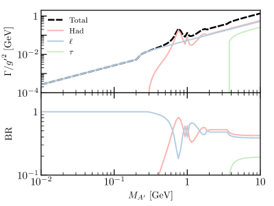
Figure 3: We plot the partial widths and the branching ratios of the dark photon for different channels of decay, as denoted in the legend. The black dashed line in the top panel indicates the total width of the particle. We have plotted a scaled version of the decay width to remove the dependence on the coupling.

With the estimate for detector efficiencies and the differential cross section in hand, we can now derive the projected limits for the dark photon. The dark photon coupling to the SM fermions are generated through its gauge kinetic mixing with the photon Holdom:1985ag . In the ‘original’ basis (hatted), where the kinetic sector of the photon and the $A^{\prime}$ is not canonically diagonalized, the Lagrangian for the dark photon is given by:

$$\mathcal{L} =-\frac{1}{4}\hat{F}^{\prime}_{\mu\nu}{\hat{F}^{\prime}}_{\mu\nu}-\frac{\epsilon}{2}\hat{F}^{\prime}_{\mu\nu}\hat{F}^{\mu\nu}\,.$$ (16)

Here, $\hat{F}_{\mu\nu}=\partial_{\mu}\hat{A}_{\nu}-\partial_{\nu}\hat{A}_{\mu}$ and $\hat{F}^{\prime}_{\mu\nu}=\partial_{\mu}\hat{A}^{\prime}_{\nu}-\partial_{\nu}\hat{A}^{\prime}_{\mu}$ are the field-strength tensors corresponding to the photon and the dark photon fields respectively. To go to the canonically orthonormalized basis, we perform the following non-unitary transformation on the photon and the dark photon fields:

$$\begin{pmatrix}\hat{A}_{\mu}\\ \hat{A}_{\mu}^{\prime}\end{pmatrix} =\begin{pmatrix}1&-\epsilon\\ 0&1\end{pmatrix}\begin{pmatrix}A_{\mu}\\ A_{\mu}^{\prime}\end{pmatrix}.$$ (17)

As a result of this transformation, the dark photon in the diagonal basis couples to all the photon currents with a strength that is proportional to the electric charges:

$$\mathcal{L}_{\mathrm{DP}} =e\epsilon\sum_{f}q_{f}A^{\prime}_{\mu}\bar{f}\gamma^{\mu}f\,,$$ (18)

where $q_{f}$ is the electric charge of the fermion $f$ and $e$ is the QED coupling. Note, for the DP case, the effective $A^{\prime}$ coupling strength is $g^{\prime}=\epsilon e$. It is straightforward to check that this basis transformation keeps the photon mass, in the new basis, equal to zero. From Eq. 18 we can clearly see that $g_{v}^{e}=-1$ for the dark photon, determining its differential cross section and its partial widths to different channels. In Fig. 3, we plot the partial widths of the dark photon along with the branching fractions for the available channels, as functions of the dark photon mass, $M_{A}^{\prime}$. As discussed above, we use the results given in Ref. Ilten:2018crw for the partial width to hadrons for $M_{A}^{\prime}\lesssim\Lambda_{\mathrm{QCD}}$. We have cross-checked the result with the partial width given in a SHIP note.

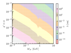
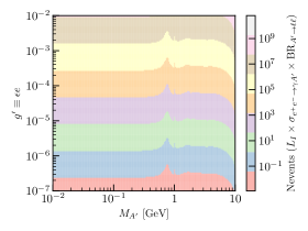
Figure 4: Left: The characteristic length of decay, $\lambda$, for different values of $M_{A^{\prime}}$ and $g^{\prime}(\equiv\epsilon e)$. The shades indicate different ranges for $\lambda$, as given by the colorbar to the right. Right: We plot the number of events produced at 50 ab^-1 of luminosity for different values of $M_{A^{\prime}}$ and $g^{\prime}$. The shades indicate different ranges for the number of events produced, as given by the colorbar to the right.

Given the width and the differential cross section of the $A^{\prime}$, we obtain its decay length distribution from the characteristic length, $\lambda=\beta\gamma c\tau$. The boost factor $\beta\gamma$ can be obtained from the magnitude of the three momentum given in Eq. 11 as $\beta\gamma=|\vec{p}|/M_{A^{\prime}}$. In the left panel of Fig. 4, we plot contours indicating the characteristic length in the ($M_{A^{\prime}},\,g^{\prime}$) plane. In the right panel of the figure, we give contours for the total number of events, $N_{\mathrm{events}}$, in the same ($M_{A^{\prime}},g^{\prime}$), to estimate the number of events produced. The number of events are calculated for an integrated luminosity of 50 ab^-1 and for $\ell\equiv e+\mu$. The cuts on the $p_{T}$ and $\eta$, as discussed in the previous section, are applied in calculating the number of events. However, no requirement on the displacement of the $A^{\prime}$ decay vertex is imposed for this plot, i.e., this is the number of events before the convolution by the VRE distribution. We do this to show the variation of the cross section with the mass and the coupling. Below, where we draw the actual exclusion limit, we use the cross section convoluted by the VRE distribution, as given in Eq. 9.

With all the relevant information in hand, we can finally present the actual limits on the parameter space from displaced vertex searches. To get the limits, we accept those ($M_{A^{\prime}},\,g^{\prime}$) points for which the number of accepted events, $N$, passes our acceptance criteria. If we assume Poisson statistics, the number of accepted events need to be greater than 2.3($\sim 3$) for a 90% C.L. exclusion limit, assuming no background. In Fig. 5, we draw the exclusion limits for integrated luminosities of 50 ab^-1 (the design luminosity of Belle II) and 200 fb^-1 (approximately the data collected by the collaboration as of writing). We draw projections for the final state of leptons ($\ell\equiv e+\mu$). From Fig. 5, we can see that once Belle II collects its machine specification of 50 ab^-1 of data, it would exclude a large part of the $M_{A^{\prime}},\,g^{\prime}$ parameter space for $10$ MeV $<M_{A^{\prime}}<500$ MeV, the region of sensitivity being demarcated by the dashed contour. It is noteworthy that this region of parameter space, that the Belle II displaced vertex searches are sensitive to, nicely complements existing limits. We have set a lower limit of $M_{A^{\prime}}$=10 MeV to stay clear of the limits set on an electrophilic light particle from BBN and CMB observables Sabti:2019mhn . For the limit at 50 ab^-1, a coupling below $g^{\prime}\sim 10^{-6}$, gives a production cross section too small to produce enough displaced vertex signatures. In the other direction, both large masses and coupling strengths make the characteristic decay length too small for the vertex to fall in our region of acceptance. These observations can also be intuited from the two panels in Fig. 4. We note that even with the data collected as of now by Belle II, it is expected to have surpassed the limits set by existing experiments in the 10 MeV $<M_{A^{\prime}}<$ 50 MeV, $2\times 10^{-5}<g^{\prime}<5\times 10^{-4}$. The existing bounds in this region come from the NA64 collaboration and the E141 collaboration, as discussed below. The projected sensitivities that we show are determined by $r_{\mathrm{min/max}}$ and $z_{\mathrm{min/max}}$, as discussed in Section 2. We have checked that the sensitivities are robust against moderate changes in the limits of $z$. We do not consider changes in the limits of $r_{\mathrm{min/max}}$, as the track reconstruction efficiency that we consider depends directly on $r_{\mathrm{min/max}}$ through the normalizing factor, as discussed in Section 2.

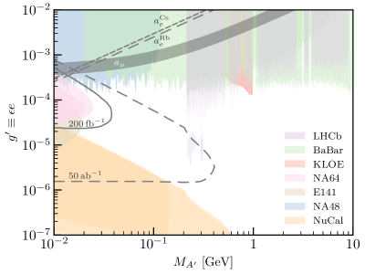
Figure 5: The dashed grey line demarcates the outer boundaries of the projected limits for Belle II sensitivity to displaced searches for the dark photon model at an integrated luminosity of 50 ab^-1, with the dark photon decaying to a lepton pair ($e$ or $\mu$). The solid grey line indicates the same but for an integrated luminosity of 200 fb^-1. The regions shaded in different colors reflect bounds from existing experiments, with the colors used for different experiments indicated in the legend. The regions of parameter space consistent with the latest measurement of $\Delta a_{\mu}$ has been shaded in grey and labelled. Also shown are the contours which satisfy the $a_{e}$ measurements using Rb and Cs.

Along with the projected limits from Belle II, in Fig. 5 we also plot existing limits on the DP parameter space from different experiments. A list of these experiments, along with short descriptions, are given in Section 1. We have used DarkCast, the companion package of Ref. Ilten:2018crw , to recast the limits from existing experiments to the $A^{\prime}$ parameter space. For the existing bounds, we have only shown those limits which are the strongest. The bounds displayed are listed below. In red, we show the bounds reported by the KLOE experiment KLOE-2:2018kqf . Bounds coming from prompt and displaced (the ‘islands’ in the middle of the plot) searches by the LHCb collaboration LHCb:2017trq ; LHCb:2019vmc have been shown in violet. The bounds from the BaBar experiment (prompt) BaBar:2014zli ; BaBar:2016sci ; BaBar:2017tiz , covering most of the mass region in consideration, have been given in green. The NA48/2 collaboration’s search for dark photons in $\pi^{0}$ decays gives the strongest bound below the $\pi^{0}$ mass NA482:2015wmo , as shown in blue. The strongest constraint from existing displaced searches Tsai:2019buq comes from the $\nu$-Calorimeter I (NuCal) experiment Blumlein:1990ay ; Blumlein:1991xh , as shown in orange. We have not shown the bounds coming from other displaced vertex searches, e.g., by the E137 collaboration Bjorken:2009mm ; Andreas:2012mt or that at Orsay Davier:1989wz , as the NuCal bound supersedes the bounds coming from both these experiments. In brown, we have given the bounds from the displaced searches by the E141 collaboration Riordan:1987aw . The pink region denotes the bound obtained by the NA64 experiment NA64:2019auh while searching for the hypothetical X(17) particle.

In Fig. 5, we have also shaded in grey the band that denotes the 2$\sigma$ limit that is consistent with the anomalous muon magnetic moment, as obtained in Ref. Bodas:2021fsy . Using dashed lines, we also denote the contours in the parameter space which are consistent with the $(g-2)_{e}$ measurements using the fine structure constant measurements from the Caesium Parker:2018vye ; Aoyama:2017uqe and Rubidium Davoudiasl:2018fbb ; Morel:2020dww atoms. We observe that the regions of parameter space that are consistent with these measurements are already ruled out by the BaBar and the NA48/2 collaborations and Belle II is sensitive to the coupling strengths corresponding to these measurements only for a very small mass range ($\lesssim$ 20 MeV).

Before concluding this section, two comments are in order. First of all, in general, the DP also mixes kinetically with the $Z$ boson that induces couplings proportional to the $Z$ couplings to the fermions. In this work, we do not consider $A^{\prime}$–$Z$ mixing of any form, only to simplify the presentation of our results. Note, we do not invoke the hierarchy of the $A^{\prime}$ and $Z$ mass scales when ignoring this mixing. Despite a hierarchical separation, other Lagrangian parameters can be tuned to have sizeable mixing (see, e.g., Ref. Bandyopadhyay:2018cwu ). Also, we are giving bounds on couplings which are extremely small $\sim 10^{-6}$. So, even when the mixing is of the order of $M_{A^{\prime}}^{2}/M_{Z}^{2}$, it would still be commensurate with the couplings we are giving bounds on. Secondly, we generally invoke dark photons as portals between the SM and some dark sector. Therefore, the typical dark photon has couplings to dark sector particles. The presence of a dark photon decay channel to dark sector particles in effect only adds an additional contribution to the total width of the dark photon, scaling the branching ratios and the characteristic decay length of the dark photon. The modification to the width and branching ratios depend on the masses of the dark sector particles and makes the analysis model dependent. Hence, for the sake of benchmarking, we do not include any dark sector particles in our work. Modifications to decay widths due to dark sector particles and modifications to coupling strengths due to $A^{\prime}$–$Z$ mixing etc. can easily be introduced in an analysis that recasts these results to a different model.

4 Models of gauged $Z^{\prime}$

Models where the anomaly free gauge symmetries of the SM are gauged, viz. $L_{\mu}-L_{\tau}$, $L_{e}-L_{\mu}$, $L_{\tau}-L_{e}$, and $B-L$, are extremely popular due to a variety of reasons, some of which we have mentioned in the introduction. In this section, we discuss the limits on these models and the model of the ‘protophobic’ force (see Ref. Feng:2016ysn , also discused below). Among these, the $L_{\mu}-L_{\tau}$ model stands out by virtue of not interacting with the first generation of fermions at leading order. This also means that its production at electron colliders is suppressed, giving signatures different from the rest. Hence, we discuss the $L_{\mu}-L_{\tau}$ model in some detail, before moving on to the other models.

4.1 $Z^{\prime}$ with $L_{\mu}-L_{\tau}$ symmetry

In $L_{\mu}-L_{\tau}$ models, interactions to the first generation fermions are generated through kinetic mixing between the $Z^{\prime}$ boson corresponding to the gauged $U(1)_{L_{\mu}-L_{\tau}}$ and the SM photon. This allows us to give projections on variants of this model from the Belle II experiment.

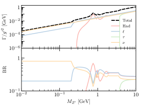
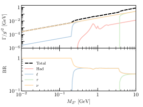
Figure 6: Partial decay widths and branching ratios for the $L_{\mu}-L_{\tau}$ $Z^{\prime}$ boson. Left: for $r_{f}=0.5$. Right: for $g_{v}^{e}/g_{v}^{\mu}=0.1$. See text for details.

In the basis where the gauge kinetic sector is not diagonal, the $Z^{\prime}$ couples to the fermions with a charge proportional to the difference between the muon lepton number and the tau lepton number. The corresponding interaction Lagrangian is given by:

$$\mathcal{L}_{Z^{\prime}}=g_{L_{\mu}-L_{\tau}}\left(\bar{\ell}_{\mu}\gamma^{\alpha}\ell_{\mu}+\bar{\mu}_{R}\gamma^{\alpha}\mu_{R}-\{\mu\rightarrow\tau\}\right)Z^{\prime}_{\alpha}\;,$$ (19)

where $\ell_{\mu}$ is the left-handed muon doublet. However, there is a gauge kinetic mixing term, between the $Z^{\prime}$ and the photon, of the form:

$$\mathcal{L}_{Z^{\prime}}\supset\frac{\epsilon}{2}Z^{\prime}_{\mu\nu}F^{\mu\nu}\;.$$ (20)

Being a marginal operator and consistent with gauge symmetries, the kinetic mixing term would be present unless special discrete symmetries are introduced such as $\mu\leftrightarrow\tau$ and $Z^{\prime}\to-Z^{\prime}$ Dienes:1996zr ; Banerjee:2018mnw . However, even then, with fermions charged under both electromagnetism and $L_{\mu}-L_{\tau}$, kinetic mixing will be generated at one loop. The generic form of the resulting mixing is Cheung:2009qd :

$$\epsilon =\frac{eg_{L_{\mu}-L_{\tau}}}{16\pi^{2}}\sum_{f}q_{f}x_{f}\ln\left(\frac{\mu^{2}}{M_{f}^{2}}\right)\;,$$ (21)

where $x_{f}$ and $M_{f}$ are the charge and the mass of the fermion $f$ in the loop, and $\mu$ is the scale of renormalization. Clearly, with many fermions (not necessarily from the SM spectrum) in the loop and with large logs, this number can be quite large, around $10^{-1}$ (see, e.g., Ref. Gherghetta:2019coi ). In this work, we take a model agnostic approach and treat the kinetic mixing as a free parameter. This term induces universal couplings between $Z^{\prime}$ and the SM fermions, including electrons, in a way exactly similar to the dark photon case. We take a hierarchical separation between the coupling of the $L_{\mu}-L_{\tau}$ boson to muons and taus, as compared to all other fermions:

$$|g_{v}^{f}| =r_{f}\,|g_{v}^{\mu/\tau}|,\;\forall f\notin\{\mu,\tau\}\,,$$ (22)

where $g_{L_{\mu}-L_{\tau}}\cdot\,g_{v}^{f}$ is the coupling of the $Z^{\prime}$ boson to the $f$ fermion. In Fig. 6, we plot the branching ratios and partial widths for $r_{f}=0.5$ and $r_{f}=0.1$. In Fig. 7, we show the limits for the same two values of $r_{f}$. As is evident from the figure, the former case is similar to the dark photon. However, the latter shows interesting deviations from the dark photon limits and merits additional comments.

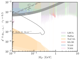
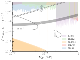
Figure 7: Similar to Fig. 5, the black contour can be probed with displaced vertex searches at Belle II for a $L_{\mu}-L_{\tau}$ gauge boson with $r_{f}=0.5$ (left) and $r_{f}=0.1$ (right). As is evident for the $r_{f}=0.1$ case, smaller values of the electron coupling reduces the production and hence relaxes the bound.

For the $r_{f}=0.1$ case, the experiment is sensitive to two disjointed regions of the parameter space. We discuss the contour in the lower mass regions first, and then move on to the ‘island’. The sensitivity region for $M_{Z^{\prime}}\lesssim 80$ MeV shows deviations from the dark photon case for two reasons. First of all, the production from $e^{+}e^{-}$ is governed by the coupling strength to electrons, therefore, is suppressed by $r_{f}^{2}$. As a result, the bound starts from larger coupling values compared to the dark photon case. Also, in this region, decay to muons is kinematically forbidden and that to electrons is controlled by the same sub-dominant $r_{f}^{2}$. Hence, the dominant branching is to neutrinos. This can also be seen from the right panel of Fig. 6, where we plot the partial widths and branching ratios for this model. Notice that the sensitivity for the $r_{f}=0.1$ case extends to larger values of $g^{\prime}$, compared to the DP case (or the $r_{f}=0.5$ case). The reason is two fold. Firstly, the coupling to electrons is suppressed by the additional $r_{f}$ factor. This implies, that we need larger $g^{\prime}$ values to get a cross section equal to the DP case. Secondly, the $r_{f}$ suppression to the coupling leads to suppressed decay lengths. Hence, for larger values of $g^{\prime}$ the decay length is still large enough for displaced searches to be sensitive. The most interesting consequence of this is that the Belle II sensitivity region ends up covering a large region of the parameter space that is compatible with the $(g-2)_{\mu}$ anomaly. We note, unlike the DP case, where the $a_{\mu}$ region is mostly ruled out by NA48 NA482:2015wmo and BaBar exclusions BaBar:2014zli ; BaBar:2016sci ; BaBar:2017tiz , it is the Belle II exclusion that has the potential to rule out most of the $a_{\mu}$ region for this model. Finally, we see that the experiment is sensitive to a small island of parameter space just above the 2$\mu$ threshold. The reason for this is that at this threshold the cross section times branching ratio to two leptons gets an enhancement due to the opening up of the muon channel for the $Z^{\prime}$ to decay to. As a result, displaced vertex searches become sensitive for a small slice of mass before losing sensitivity as the inclusion of the $\mu$ channel increases the total decay width to an extent that displaced vertex searches become untenable.

4.2 Other Models

In this subsection, we discuss the projections for displaced vertex searches at Belle II for a few other models of interest. As the analysis is the same as that discussed before, we just discuss the limits for these models. The models we discuss are the $L_{e}-L_{\mu/\tau}$ models, the $B-L$ model, and the protophobic model. As all of these models couple to first generation fermions, the limits are similar across them, with minor differences that we discuss in brief.

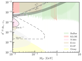
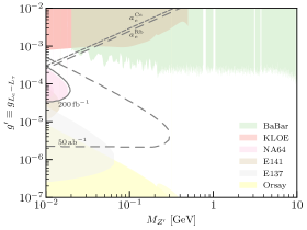
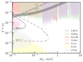
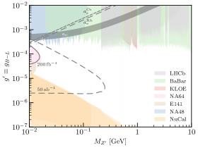
Figure 8: In the top left and right panels, we plot the projected limits in the parameter space of the $L_{e}-L_{\mu}$ and the $L_{e}-L_{\tau}$ models respectively. In the bottom left panel and the bottom right panels, we draw the same for the protophobic model and the $B-L$ model respectively.

In the top two panels of Fig. 8, we plot the Belle II projections and existing limits for the $L_{e}-L_{\mu}$ model (left) and the $L_{e}-L_{\tau}$ model (right). In these models, the gauge boson couples to the electron at leading order. As a result, the projected limits extend for a large portion of the parameter space. Note, we do not assume sizeable kinetic mixing for these models. Needless to say, large kinetic mixing coefficients can be generated for these models too, in which case these projections will be modified. The existing bounds for the both the $L_{e}-L_{i}$ models are somewhat different from the dark photon case. As the $Z^{\prime}$ in these models do not interact with hadrons at leading order, there is no bound from the NuCal (proton beam) data. Instead, the strongest displaced vertex bounds, in regions of small coupling, come from the electron beam dump data as collected at Orsay Davier:1989wz and by the E137 collaboration Bjorken:1988as . Also, LHCb or NA48 data does not give limits on the parameter space of these models, with the large coupling region only constrained by BaBar BaBar:2014zli ; BaBar:2016sci ; BaBar:2017tiz and KLOE KLOE-2:2018kqf .

The protophobic and the $B-L$ models differ from the other two in the sense that in these models, the $Z^{\prime}$ has $\mathcal{O}(1)$ couplings to the quarks. The protophobic model was postulated as an explanation of the ATOMKI anomaly Krasznahorkay:2018snd ; Krasznahorkay:2021joi . The gauge boson in the model, $X(17)$, couples universally and vectorially to the three generations. The couplings to the up-type quarks, down-type quarks, charged leptons, and neutrinos are $-1/3,2/3,-1$, and 0 respectively. With these couplings, it is easy to see that the net charge of the proton is zero. In the bottom left panel of Fig. 8, we show the projected limits in the parameter space of this model. The important thing to note from the figure is that at 200 fb^-1, i.e., the amount of data Belle II is expected to have collected by now, the Belle II displaced limit gives a stronger bound than the limits set by the NA64 collaboration in a dedicated search of this particle NA64:2019auh , as given by the pink region. That is, an analysis of the present Belle II data against the displaced vertex hypothesis has the potential to reproduce the results of the NA64 collaboration and in the process rule out (or discover) the X(17) explanation of the ATOMKI anomaly. As for existing beam dump searches, although the X boson interacts with quarks, there is no strong bound from NuCal in this case, as the quark couplings of the X boson are engineered specifically to have no interaction with the proton. The strongest displaced constraints for the X particle comes from the electron beam experiments at Orsay and E137. Finally, in the bottom right panel of Fig. 8, we plot the projected limits for the $B-L$ model for two integrated luminosities, $L_{I}=200$ fb^-1 and $L_{I}=50$ ab^-1. From the figure we see that the limit and the existing bounds are more or less similar to those for the dark photon. This is expected, as the couplings of the vector boson in the two models are similar.

5 Conclusion

Displaced vertex searches at the Belle II experiment has enormous potential to scrutinize a large part of the parameter space of models with a vector boson with mass $\lesssim 0.5$ GeV. Our projections, both for the Belle II design luminosity of 50 ab^-1 and the expected current luminosity of 200 fb^-1, show that the collaboration should consider analysing there data to test the displaced vertex hypothesis. Such searches not only have the possibility to probe as yet uncharted territories in the light vector boson parameter space, but also to test specific scenarios invoked as explanations to hints of new physics. Such scenarios include, but are not limited to, portals to dark matter, new vector bosons to solve the $(g-2)_{\mu}$ anomaly, and the protophobic boson postulated to solve the ATOMKI anomaly.

Note Added

While finishing our work, Ref. Ferber:2022ewf appeared which also looked at the displaced vertex searches for a dark photon at Belle II. We present a more analytical and detailed estimation of the efficiency pertaining to displaced vertices. Our DP results overlap with the findings of Ref. Ferber:2022ewf for some regions of parameter space. We also extend the analysis for light $Z^{\prime}$ models where displaced vertex searches can probe significant part of the parameter space.

- (1) Belle-II collaboration, The Belle II Physics Book, PTEP 2019 (2019) 123C01 [1808.10567].
- (2) SuperKEKB collaboration, SuperKEKB Collider, Nucl. Instrum. Meth. A 907 (2018) 188 [1809.01958].
- (3) BaBar collaboration, D. Boutigny et al., The BABAR physics book: Physics at an asymmetric factory (10, 1998), 10.2172/979931.
- (4) Belle collaboration, Physics Achievements from the Belle Experiment, PTEP 2012 (2012) 04D001 [1212.5342].
- (5) C.O. Dib, J.C. Helo, M. Nayak, N.A. Neill, A. Soffer and J. Zamora-Saa, Searching for a sterile neutrino that mixes predominantly with at factories, Phys. Rev. D 101 (2020) 093003 [1908.09719].
- (6) E. Bertholet, S. Chakraborty, V. Loladze, T. Okui, A. Soffer and K. Tobioka, Heavy QCD Axion at Belle II: Displaced and Prompt Signals, 2108.10331.
- (7) S. Chakraborty, M. Kraus, V. Loladze, T. Okui and K. Tobioka, Heavy QCD axion in b→s transition: Enhanced limits and projections, Phys. Rev. D 104 (2021) 055036 [2102.04474].
- (8) M. Duerr, T. Ferber, C. Hearty, F. Kahlhoefer, K. Schmidt-Hoberg and P. Tunney, Invisible and displaced dark matter signatures at Belle II, JHEP 02 (2020) 039 [1911.03176].
- (9) T. Ferber, C. Garcia-Cely and K. Schmidt-Hoberg, Belle II sensitivity to long-lived dark photons, 2202.03452.
- (10) I. Galon, D. Shih and I.R. Wang, Dark Photons and Displaced Vertices at the MUonE Experiment, 2202.08843.
- (11) G. Abbiendi, Status of the MUonE experiment, in 10th International Conference on New Frontiers in Physics, 1, 2022 [2201.13177].
- (12) C. Boehm and P. Fayet, Scalar dark matter candidates, Nucl. Phys. B 683 (2004) 219 [hep-ph/0305261].
- (13) P. Fayet, Light spin 1/2 or spin 0 dark matter particles, Phys. Rev. D 70 (2004) 023514 [hep-ph/0403226].
- (14) L.B. Okun, Limits of Electrodynamics: Paraphotons?, Sov. Phys. JETP 56 (1982) 502.
- (15) P. Galison and A. Manohar, Two Z’s or not two Z’s?, Phys. Lett. B 136 (1984) 279.
- (16) B. Holdom, Two U(1)’s and Epsilon Charge Shifts, Phys. Lett. B 166 (1986) 196.
- (17) P. Fayet, On the Search for a New Spin 1 Boson, Nucl. Phys. B 187 (1981) 184.
- (18) R. Foot, New Physics From Electric Charge Quantization?, Mod. Phys. Lett. A 6 (1991) 527.
- (19) X.G. He, G.C. Joshi, H. Lew and R.R. Volkas, NEW Z-prime PHENOMENOLOGY, Phys. Rev. D 43 (1991) 22.
- (20) X.-G. He, G.C. Joshi, H. Lew and R.R. Volkas, Simplest Z-prime model, Phys. Rev. D 44 (1991) 2118.
- (21) M. Kadastik, K. Kannike and M. Raidal, Dark Matter as the signal of Grand Unification, Phys. Rev. D 80 (2009) 085020 [0907.1894].
- (22) M. Frigerio and T. Hambye, Dark matter stability and unification without supersymmetry, Phys. Rev. D 81 (2010) 075002 [0912.1545].
- (23) J. Heeck and S. Patra, Minimal Left-Right Symmetric Dark Matter, Phys. Rev. Lett. 115 (2015) 121804 [1507.01584].
- (24) T. Bandyopadhyay and A. Raychaudhuri, Left–right model with TeV fermionic dark matter and unification, Phys. Lett. B 771 (2017) 206 [1703.08125].
- (25) P. Foldenauer, Light dark matter in a gauged model, Phys. Rev. D 99 (2019) 035007 [1808.03647].
- (26) E. Ma, D.P. Roy and S. Roy, Gauged L(mu) - L(tau) with large muon anomalous magnetic moment and the bimaximal mixing of neutrinos, Phys. Lett. B 525 (2002) 101 [hep-ph/0110146].
- (27) M. Pospelov, Secluded U(1) below the weak scale, Phys. Rev. D 80 (2009) 095002 [0811.1030].
- (28) J. Heeck and W. Rodejohann, Gauged Symmetry at the Electroweak Scale, Phys. Rev. D 84 (2011) 075007 [1107.5238].
- (29) A.J. Buras, A. Crivellin, F. Kirk, C.A. Manzari and M. Montull, Global analysis of leptophilic Z’ bosons, JHEP 06 (2021) 068 [2104.07680].
- (30) Muon g-2 collaboration, Final Report of the Muon E821 Anomalous Magnetic Moment Measurement at BNL, Phys. Rev. D 73 (2006) 072003 [hep-ex/0602035].
- (31) T. Aoyama et al., The anomalous magnetic moment of the muon in the Standard Model, Phys. Rept. 887 (2020) 1 [2006.04822].
- (32) Muon g-2 collaboration, Measurement of the Positive Muon Anomalous Magnetic Moment to 0.46 ppm, Phys. Rev. Lett. 126 (2021) 141801 [2104.03281].
- (33) S. Borsanyi et al., Leading hadronic contribution to the muon magnetic moment from lattice QCD, Nature 593 (2021) 51 [2002.12347].
- (34) Muon g-2 collaboration, Muon (g-2) Technical Design Report, 1501.06858.
- (35) M. Abe et al., A New Approach for Measuring the Muon Anomalous Magnetic Moment and Electric Dipole Moment, PTEP 2019 (2019) 053C02 [1901.03047].
- (36) R.H. Parker, C. Yu, W. Zhong, B. Estey and H. Müller, Measurement of the fine-structure constant as a test of the Standard Model, Science 360 (2018) 191 [1812.04130].
- (37) T. Aoyama, T. Kinoshita and M. Nio, Revised and Improved Value of the QED Tenth-Order Electron Anomalous Magnetic Moment, Phys. Rev. D 97 (2018) 036001 [1712.06060].
- (38) H. Davoudiasl and W.J. Marciano, Tale of two anomalies, Phys. Rev. D 98 (2018) 075011 [1806.10252].
- (39) L. Morel, Z. Yao, P. Cladé and S. Guellati-Khélifa, Determination of the fine-structure constant with an accuracy of 81 parts per trillion, Nature 588 (2020) 61.
- (40) M. Graham, C. Hearty and M. Williams, Searches for Dark Photons at Accelerators, Ann. Rev. Nucl. Part. Sci. 71 (2021) 37 [2104.10280].
- (41) P. Fayet, U-boson production in e+ e- annihilations, psi and Upsilon decays, and Light Dark Matter, Phys. Rev. D 75 (2007) 115017 [hep-ph/0702176].
- (42) BaBar collaboration, Search for a Dark Photon in Collisions at BaBar, Phys. Rev. Lett. 113 (2014) 201801 [1406.2980].
- (43) BaBar collaboration, Search for a muonic dark force at BABAR, Phys. Rev. D 94 (2016) 011102 [1606.03501].
- (44) BaBar collaboration, Search for Invisible Decays of a Dark Photon Produced in Collisions at BaBar, Phys. Rev. Lett. 119 (2017) 131804 [1702.03327].
- (45) Y. Jho, Y. Kwon, S.C. Park and P.-Y. Tseng, Search for muon-philic new light gauge boson at Belle II, JHEP 10 (2019) 168 [1904.13053].
- (46) A. Anastasi et al., Limit on the production of a low-mass vector boson in , with the KLOE experiment, Phys. Lett. B 750 (2015) 633 [1509.00740].
- (47) KLOE-2 collaboration, Combined limit on the production of a light gauge boson decaying into and , Phys. Lett. B 784 (2018) 336 [1807.02691].
- (48) BESIII collaboration, Dark Photon Search in the Mass Range Between 1.5 and 3.4 GeV/, Phys. Lett. B 774 (2017) 252 [1705.04265].
- (49) LHCb collaboration, Search for Dark Photons Produced in 13 TeV Collisions, Phys. Rev. Lett. 120 (2018) 061801 [1710.02867].
- (50) LHCb collaboration, Search for Decays, Phys. Rev. Lett. 124 (2020) 041801 [1910.06926].
- (51) NA48/2 collaboration, Search for the dark photon in decays, Phys. Lett. B 746 (2015) 178 [1504.00607].
- (52) NA62 collaboration, Search for production of an invisible dark photon in decays, JHEP 05 (2019) 182 [1903.08767].
- (53) CHARM collaboration, Search for Axion Like Particle Production in 400-GeV Proton - Copper Interactions, Phys. Lett. B 157 (1985) 458.
- (54) Y.-D. Tsai, P. deNiverville and M.X. Liu, Dark Photon and Muon Inspired Inelastic Dark Matter Models at the High-Energy Intensity Frontier, Phys. Rev. Lett. 126 (2021) 181801 [1908.07525].
- (55) NOMAD collaboration, Search for a new gauge boson in pi0 decays, Phys. Lett. B 428 (1998) 197 [hep-ex/9804003].
- (56) S.N. Gninenko, Stringent limits on the decay from neutrino experiments and constraints on new light gauge bosons, Phys. Rev. D 85 (2012) 055027 [1112.5438].
- (57) J. Blumlein et al., Limits on neutral light scalar and pseudoscalar particles in a proton beam dump experiment, Z. Phys. C 51 (1991) 341.
- (58) J. Blumlein et al., Limits on the mass of light (pseudo)scalar particles from Bethe-Heitler e+ e- and mu+ mu- pair production in a proton - iron beam dump experiment, Int. J. Mod. Phys. A 7 (1992) 3835.
- (59) J.D. Bjorken, S. Ecklund, W.R. Nelson, A. Abashian, C. Church, B. Lu et al., Search for Neutral Metastable Penetrating Particles Produced in the SLAC Beam Dump, Phys. Rev. D 38 (1988) 3375.
- (60) E.M. Riordan et al., A Search for Short Lived Axions in an Electron Beam Dump Experiment, Phys. Rev. Lett. 59 (1987) 755.
- (61) A. Konaka et al., Search for Neutral Particles in Electron Beam Dump Experiment, Phys. Rev. Lett. 57 (1986) 659.
- (62) M. Davier and H. Nguyen Ngoc, An Unambiguous Search for a Light Higgs Boson, Phys. Lett. B 229 (1989) 150.
- (63) APEX collaboration, Search for a New Gauge Boson in Electron-Nucleus Fixed-Target Scattering by the APEX Experiment, Phys. Rev. Lett. 107 (2011) 191804 [1108.2750].
- (64) H. Merkel et al., Search at the Mainz Microtron for Light Massive Gauge Bosons Relevant for the Muon g-2 Anomaly, Phys. Rev. Lett. 112 (2014) 221802 [1404.5502].
- (65) NA64 collaboration, Improved limits on a hypothetical X(16.7) boson and a dark photon decaying into pairs, Phys. Rev. D 101 (2020) 071101 [1912.11389].
- (66) J.L. Feng, B. Fornal, I. Galon, S. Gardner, J. Smolinsky, T.M.P. Tait et al., Particle physics models for the 17 MeV anomaly in beryllium nuclear decays, Phys. Rev. D 95 (2017) 035017 [1608.03591].
- (67) A.J. Krasznahorkay et al., New results on the 8Be anomaly, J. Phys. Conf. Ser. 1056 (2018) 012028.
- (68) A.J. Krasznahorkay, M. Csatlós, L. Csige, J. Gulyás, A. Krasznahorkay, B.M. Nyakó et al., New anomaly observed in He4 supports the existence of the hypothetical X17 particle, Phys. Rev. C 104 (2021) 044003 [2104.10075].
- (69) P. Fayet, The Fifth Interaction in Grand Unified Theories: A New Force Acting Mostly on Neutrons and Particle Spins, Phys. Lett. B 172 (1986) 363.
- (70) S. Tulin, New weakly-coupled forces hidden in low-energy QCD, Phys. Rev. D 89 (2014) 114008 [1404.4370].
- (71) M. Bauer, P. Foldenauer and J. Jaeckel, Hunting All the Hidden Photons, JHEP 07 (2018) 094 [1803.05466].
- (72) P. Ilten, Y. Soreq, M. Williams and W. Xue, Serendipity in dark photon searches, JHEP 06 (2018) 004 [1801.04847].
- (73) N. Sabti, J. Alvey, M. Escudero, M. Fairbairn and D. Blas, Refined Bounds on MeV-scale Thermal Dark Sectors from BBN and the CMB, JCAP 01 (2020) 004 [1910.01649].
- (74) J.D. Bjorken, R. Essig, P. Schuster and N. Toro, New Fixed-Target Experiments to Search for Dark Gauge Forces, Phys. Rev. D 80 (2009) 075018 [0906.0580].
- (75) S. Andreas, C. Niebuhr and A. Ringwald, New Limits on Hidden Photons from Past Electron Beam Dumps, Phys. Rev. D 86 (2012) 095019 [1209.6083].
- (76) A. Bodas, R. Coy and S.J.D. King, Solving the electron and muon anomalies in models, Eur. Phys. J. C 81 (2021) 1065 [2102.07781].
- (77) T. Bandyopadhyay, G. Bhattacharyya, D. Das and A. Raychaudhuri, Reappraisal of constraints on models from unitarity and direct searches at the LHC, Phys. Rev. D 98 (2018) 035027 [1803.07989].
- (78) K.R. Dienes, C.F. Kolda and J. March-Russell, Kinetic mixing and the supersymmetric gauge hierarchy, Nucl. Phys. B 492 (1997) 104 [hep-ph/9610479].
- (79) H. Banerjee and S. Roy, Signatures of supersymmetry and gauge bosons at Belle-II, Phys. Rev. D 99 (2019) 035035 [1811.00407].
- (80) C. Cheung, J.T. Ruderman, L.-T. Wang and I. Yavin, Kinetic Mixing as the Origin of Light Dark Scales, Phys. Rev. D 80 (2009) 035008 [0902.3246].
- (81) T. Gherghetta, J. Kersten, K. Olive and M. Pospelov, Evaluating the price of tiny kinetic mixing, Phys. Rev. D 100 (2019) 095001 [1909.00696].