Influence of Asymmetric Parameters in Higher-Order Coupling With Bimodal Frequency Distribution

Abstract

We investigate the phase diagram of the Sakaguchi-Kuramoto model with a higher order interaction along with the traditional pairwise interaction. We also introduce asymmetry parameters in both the interaction terms and investigate the collective dynamics and their transitions in the phase diagrams under both unimodal and bimodal frequency distributions. We deduce the evolution equations for the macroscopic order parameters and eventually derive pitchfork and Hopf bifurcation curves. Transition from the incoherent state to standing wave pattern is observed in the presence of the unimodal frequency distribution. In contrast, a rich variety of dynamical states such as the incoherent state, partially synchronized state-I, partially synchronized state-II, and standing wave patterns and transitions among them are observed in the phase diagram, via various bifurcation scenarios including saddle-node and homoclinic bifurcations, in the presence of bimodal frequency distribution. Higher order coupling enhances the spread of the bistable regions in the phase diagrams and also leads to the manifestation of bistability between incoherent and partially synchronized states even with unimodal frequency distribution, which is otherwise not observed with the pairwise coupling. Further, the asymmetry parameters facilitate the onset of several bistable and multistable regions in the phase diagrams. Very large values of the asymmetry parameters allow the phase diagrams to admit only the monostable dynamical states.

Keywords: Higher-Order Coupling, Sakaguchi-Kuramoto model, Bifurcation

I Introduction

Coupled nonlinear oscillators constitute an excellent framework to unravel and understand a plethora of intriguing collective dynamics/patterns observed in a wide variety of natural systems Kuramoto:1984 ; winfree ; Strogatz:2000 ; Pikovsky:2001 ; Acebron:2005 . In particular, the phenomenon of synchronization has been widely studied in the past two decades due to its manifestation in several natural and man-made systems Pikovsky:2001 ; Acebron:2005 ; Gupta:2014 ; Gupta:2018 . For instance, collective synchrony includes synchronized firing of cardiac pacemaker cells Peskin:1975 , synchronous emission of light pulses by groups of fireflies Buck:1988 , chirping of crickets Walker:1969 , synchronization in ensembles of electrochemical oscillators Kiss:2002 , synchronization in human cerebral connectome Schmidt:2015 , and synchronous clapping of audience Neda:2000 . Incredibly, the Kuramoto model has been employed as a paradigmatic model to understand diverse emerging nonlinear phenomena across various disciplines, including physics, biology, chemistry, ecology, electrical engineering, neuroscience, and sociology Kuramoto:1984 ; winfree ; Strogatz:2000 ; Pikovsky:2001 ; Acebron:2005 ; Pikovsky:2001 , as it allows for an exact analytical treatment in most cases in explaining macroscopic dynamics.

The Kuramoto model comprises of $N$ globally-coupled phase oscillators with distributed natural frequencies interacting symmetrically with one another through the sine of their phase differences. Considering symmetric interaction in the dynamics is only an approximation that may simplify the theoretical analysis, which indeed may fail to capture important phenomena occurring in real systems. In contrast to the standard Kuramoto model, interactions between oscillators may be asymmetric, in general. For example, asymmetric interaction leads to novel features such as families of traveling wave states Iatsenko:2013 ; Petkoski:2013 , glassy states and super-relaxation Iatsenko:2014 , and so forth, and has been invoked to discuss coupled circadian neurons Gu:2016 , dynamic interactions Yang:2020 ; Sakaguchi:1988 , etc. A generalization of the Kuramoto model that accounts for asymmetric interaction is the so-called Sakaguchi-Kuramoto model, whose dynamics can be described by the equation of motion Sakaguchi:1986 ; Oleh-SK-1 ; Oleh-SK-2

$$\frac{{\rm d}\theta_{j}}{{\rm d}t}=\omega_{j}+\frac{K}{N}\sum_{k=1}^{N}\sin(\theta_{k}-\theta_{j}+\alpha),$$ (1)

where $0\leq\alpha<\pi/2$ is the asymmetry parameter. The model (1) and its variants have been successfully employed to study a variety of dynamical scenarios such as disordered Josephson series array Wiesenfeld:1996 , multiplex network sj:1 ; sj:2 ; sj:3 ; sj:4 , time-delayed interactions Yeung:1999 , hierarchical populations of coupled oscillators Pikovsky:2008 , chaotic transients Wolfrum:2011 , dynamics of pulse-coupled oscillators Pazo:2014 , etc.

Majority of the investigations in either Kuramoto or Sakaguchi-Kuramoto models were carried out with pairwise interactions. Nevertheless, in many realistic systems, such as Huygens pendulum, neuronal oscillators, genetic networks, globally coupled photochemical oscillators, etc.,  o:2 ; o:3 ; o:4 ; o:5 higher order Fourier harmonics in the coupling function ho:1 ; Bick2011 or higher order couplings Bick2016 ; ho:2 play a predominant role in shaping the collective dynamics. Recently, it has been shown that higher order couplings lead to added nonlinearity in the macroscopic system dynamics that induce abrupt synchronization transitions via hysteresis and bistability o:5 . Further, higher order interactions are shown to stabilize strongly synchronized states even when the pairwise coupling is repulsive, which is otherwise unstable ho:3 . Abrupt or explosive synchronization was shown to manifest in networks in which the degrees of the nodes are positively correlated with the frequency of the node dynamics. In contrast, higher oder interactions are shown to be responsible for the rapid switching to synchronization, leading to explosive synchronization, in many biological and other systems without the need for particular correlation mechanism between the oscillators and the topological structure ho:4 .

In this work, we unravel the influence of the asymmetry parameters in the phase diagram of the Sakaguchi-Kuramoto model with pairwise and higher order couplings under the influence of both the unimodal and bimodal distributions of the natural frequencies. We employ two different asymmetry parameters, namely $\alpha_{1}$ in the pairwise coupling and $\alpha_{2}$ in the higher order coupling. The effect of interplay of the asymmetry parameters and the higher order coupling on the collective dynamical behavior of the Sakaguchi-Kuramoto model will be captured in the two parameter phase diagrams. We consider five different cases, namely (i) $\alpha_{1}$ = $\alpha_{2}$ = 0 (ii) $\alpha_{1}$ = $\alpha_{2}~{}\neq~{}0$, (iii) $\alpha_{1}~{}\neq~{}0$; $\alpha_{2}$ = 0, (iv) $\alpha_{2}~{}\neq~{}0$; $\alpha_{1}$ = 0, and (v) $\alpha_{1}~{}>0~{}\&~{}\alpha_{2}>0$. to unravel the emerging collective dynamics and their respective phase diagrams. We observe incoherent state (IC), partially synchronized state-I (PS-I), partially synchronized state-II (PS-II), and standing wave (SW) in the phase diagrams along with various bistable and multistable regions. We also deduce the evolution equations for the macroscopic order parameters by employing the Ott-Antonsen ansatz Ott:2008 ; Ott:2009 . We derive analytical stability conditions for the incoherent state, which results in the pitchfork and Hopf bifurcation curves, from the governing equations of motion of the macroscopic order parameters. Furthermore, we obtain the saddle-node and homoclinic bifurcation curves using the software package XPPAUT xpp , which leads to several bifurcation transitions across the various dynamical states. We find that the higher order coupling essentially facilitates enlargement of bistable states. Higher order coupling also facilitates the onset of the bistability between the IC and PS-I states even for the unimodal frequency distribution, a phenomenon which cannot be seen in the Sakaguchi-Kuramoto model with pairwise coupling and unimodal distribution. Furthermore, a low value of $\alpha_{1}$ for $\alpha_{2}=0$ and a large value of $\alpha_{2}$ for $\alpha_{1}=0$ facilitate the onset of PS-II and bistable region R3 (bistability between PS-I and PS-II) in the phase diagram. Very large values of $\alpha_{1}$ and $\alpha_{2}$ allow the phase diagrams to admit only the monostable dynamical states despite the fact that appropriate values of the asymmetry parameters induce bistable and multistable states. It is to be noted that bistable (multistable) regions are characterized by abrupt transitions among the dynamical states.

The paper is organized as follows. We introduce the Sakaguchi-Kuramoto model in Sec. II. We deduce the evolution equations corresponding to the macroscopic order parameters using the Ott-Antonsen ansatz in Sec. III. In Sec. IV, we illustrate the phase diagrams of the model with both unimodal and bimodal frequency distribution for various possible combinations of the asymmetry parameters $\alpha_{1}$ and $\alpha_{2}$ and discuss the dynamical transitions across various bifurcation scenarios demarcating the dynamical states in the phase diagrams. Finally, we will provide a summary and conclusions in Sec. V.

II Model

The $N$-coupled Sakaguchi-Kuramoto model with a specific higher order interaction is governed by the set of $N$ coupled first order nonlinear ordinary differential equations (ODEs),

$$\dot{\theta}_{i} \,=\omega_{i}+{k}\big{[}\frac{1}{N}\sum_{j=1}^{N}\sin(\theta_{j}-\theta_{i}-\alpha_{1})$$ (2)

$$\,+\frac{1}{N^{3}}\sum_{j=1}^{N}\sum_{k=1}^{N}\sum_{l=1}^{N}\sin(\theta_{j}+\theta_{k}-\theta_{l}-\theta_{i}-\alpha_{2})\big{]},~{}i=1,2,\ldots,N,$$

where $\theta_{i}$ is the phase of the $i$th oscillator, $\omega_{i}$ is its natural frequency, which is typically assumed to be drawn from a well behaved distribution $g(\omega)$. $\alpha_{1}$ and $\alpha_{2}$ are the asymmetry parameters of pairwise and higher order interactions, respectively. $k$ is the coupling strength of both pairwise and higher order interactions ho:1 ; ho:2 ; ho:3 ; ho:4 . The Kuramoto model with higher-order interactions is known to describe topological structures such as higher-order simplexes or a simplicial complex ex:1 ; ex:2 , which are relevant to brain dynamics, neuronal networks, and biological transport networks ex:3 ; ex:4 . In recent times, neuroscience studies have confirmed the existence of higher-order interactions between neurons. For example, astrocytes and other glial cells are thought to be a biological source of high-order interactions since they interact with hundreds of synapses and actively regulate their activity ex:5 ; ex:6 .

We consider a bimodal frequency distribution for $g(\omega)$ in our system. Specifically, we consider the Lorentzian distribution of unimodal and bimodal frequency distribution,

$$g(\omega) =\frac{\gamma}{\pi((\omega-\omega_{0})^{2}+\gamma^{2})};~{}~{}\gamma>0.$$ (3)

$$g(\omega) =\frac{\gamma}{\pi}\left[\frac{1}{((\omega-\omega_{0})^{2}+\gamma^{2})}+\frac{1}{((\omega+\omega_{0})^{2}+\gamma^{2})}\right],~{}\gamma>0.$$ (4)

Here $\gamma$ is the width parameter (half width at half maximum) of each peak and $\pm\omega_{0}$ are the location of their peaks. A more physically relevant interpretation of $\omega_{0}$ is that it defines the detuning in the system (which is proportional to the separation between the two central frequencies). Note that the form of the distribution $g(\omega)$ given in (4) is symmetric about zero. Another point to observe is that $g(\omega)$ is bimodal if and only if the peaks are sufficiently far apart compared to their widths. Specifically, one needs $\omega_{0}>\gamma/\sqrt{3}$. Otherwise, the distribution is unimodal and the classical results still apply.

III Evolution equation of the macroscopic order parameters

In the thermodynamic limit ($N\to\infty$ ), the system of equations (2) can be reduced to a finite set of macroscopic variables in terms of the macroscopic order parameters governing the dynamics of the original system of equations. In this limit, the discrete set of equations can be extended to a continuous formulation using the probability density function $f(\theta,\omega,t)$, where $f(\theta,\omega,t){\rm d}\theta$ characterizes the fraction of the oscillators with phases between $[\theta,\theta+{\rm d}\theta]$ along with the natural frequency $\omega$ at a time $t$.

The distribution is $2\pi$-periodic in $\theta$ and obeys the normalization condition

$$\int_{0}^{2\pi}{\rm d}\theta~{}f(\theta,\omega,t)=g(\omega)~{}\forall~{}\omega.$$ (5)

The evolution of $f(\theta,\omega,t)$ follows the continuity equation

$$\frac{\partial f}{\partial t}+\frac{\partial(fv)}{\partial\theta}=0,$$ (6)

where $v(\theta,\omega,t)=\frac{d\theta}{dt}$ is the angular velocity at position $\theta$ at time $t$. From Eq. (2), one can get

$$v(\theta,\omega,t)=\omega+ \frac{k}{2i}\big{[}(Ze^{-i(\theta+\alpha_{1})}-Z^{\star}e^{i(\theta+\alpha_{1})})$$

$$+ ({Z^{2}}{Z^{\star}}e^{-i(\theta+\alpha_{2})}-{Z^{\star}}^{2}Ze^{i(\theta+\alpha_{2})})\big{]},$$ (7)

where $Z(t)$ is the macroscopic order parameter defined as

$$Z=\int_{-\infty}^{\infty}g(\omega)\int_{0}^{2\pi}f(\theta,\omega,t)e^{i\theta}d\theta d\omega,$$ (8)

and $Z^{\star}$ is its complex conjugate. Expanding $f(\theta,\omega,t)$ in Fourier series, we have

$$f(\theta,\omega,t)=\frac{g(\omega)}{2\pi}\left[1+\sum_{n=1}^{\infty}\left(a_{n}(\omega,t)e^{\mathrm{i}n\theta}\right)+{\rm c.c.}\right],$$ (9)

where the prefactor of $g(\omega)$ ensures that the normalization (5) is satisfied, $a_{n}(\omega,t)$ is the $n$-th Fourier coefficient, while c.c. denotes the complex conjugation of the preceding sum within the brackets. Using the Ott-Antonsen ansatz  Ott:2008 ; Ott:2009

$$a_{n}(\omega,t)=\left[a(\omega,t)\right]^{n},$$ (10)

one can obtain,

$$\frac{\partial a}{\partial t}+i\omega a+\frac{k}{2}\big{[}(Z{a^{2}}e^{-i\alpha_{1}}-Z^{\star}e^{i\alpha_{1}})+{|Z|^{2}}({Z}{a^{2}}e^{-i\alpha_{2}}-{Z^{\star}}e^{i\alpha_{2}})\big{]},$$ (11)

where

$$Z=\int_{-\infty}^{\infty}a^{\star}(t,\omega)g(\omega)d\omega.$$ (12)

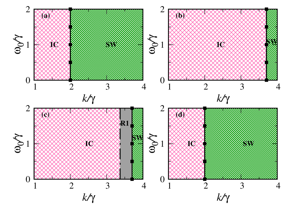
Figure 1: Phase diagrams in the ($k/\gamma-\omega_{0}/\gamma$) plane. (a) $\alpha_{1,2}$=0, (b) $\alpha_{1}=\alpha_{2}$, (c) $\alpha_{1}=1.0,\alpha_{2}=0.0$, and (d) $\alpha_{2}=1.0,\alpha_{1}=0.0$. Incoherent state and standing wave are denoted by IC and SW, respectively. Phase space with bistability (grey shaded region) between IC and SW is denoted as R1. The Hopf bifurcation (line connected by filled squares) curves are the analytical stability curves. Homoclinic (dotted-dashed line) bifurcation curve is obtained from XPPAUT.

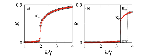
Figure 2: Order parameter (R), obtained from numerical analysis of Eq. (2) for unimodal distribution, illustrating the nature of the dynamical transitions for (a) $\alpha_{1,2}=0$; (b) $\alpha_{1}=1,\alpha_{2}=0.0$.

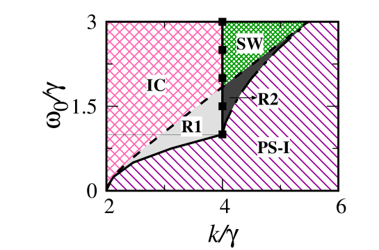
Figure 3: Phase diagram in ($k/\gamma-\omega_{0}/\gamma$) plane for $\alpha_{1}=\alpha_{2}=0$. Incoherent state, partially synchronized state-I and standing wave are denoted by IC, PS-I and SW, respectively. Phase space with bistability between IC and PS-I states is denoted as R1 and that between SW and PS-I is denoted as R2. The pitchfork (solid black), Hopf bifurcation (line connected by filled squares) and saddle-node (dashed line) curves are the analytical stability curves. Homoclinic (dotted-dashed line) bifurcation curve is obtained from XPPAUT.

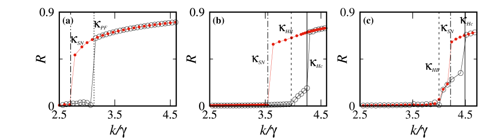
Figure 4: Order parameter (R), obtained from numerical analysis of (2) with bimodal distribution, illustrating the nature of dynamical transitions for $\alpha_{1,2}=0$ for various ratios of $\omega_{0}/\gamma$: (a) 0.75; (b) 1.5, and (c) 2.

III.1 Unimodel Frequency Distribution

The arbitrary function $a(\omega,t)$ is assumed to satisfy $|a(\omega,t)|<1$, together with the requirements that $a(\omega,t)$ may be analytically continued in the whole of the complex-$\omega$ plane and it has no singularities in the lower-half complex-$\omega$ plane. Further, $|a(\omega,t)|\to 0$ as ${\rm Im}(\omega)\to-\infty$. If these conditions are satisfied for $a(\omega,0)$, then as shown in (10), they continue to be satisfied by $a(\omega,t)$ as it evolves under Eqs. (11) and (12). Expanding the unimodal frequency distribution $g(\omega)$, Eq. (3), in partial fractions as

$$g(\omega)=\frac{1}{4\pi i}\bigg{[} \frac{1}{((\omega-\omega_{0})-i\gamma)}-\frac{1}{((\omega-\omega_{0})+i\gamma)}\bigg{]},$$ (13)

and evaluating Eq. (12) using the appropriate contour integral, the order parameter becomes,

$$Z(t)=a^{\star}(\omega_{0}-i\gamma,t).$$ (14)

Substituting the above in Eq. (11), one obtains a complex ODE, describing the evolution of the suborder parameter,

$$\frac{\partial Z}{\partial t}+(\gamma+i \omega_{0})Z+\frac{k}{2}Z\bigg{[}(|Z|^{2}e^{-i\alpha_{1}}-e^{i\alpha_{1}})$$

$$+|Z|^{2}(|Z|^{2}e^{(}-i\alpha_{2})-e^{i\alpha_{2}})\bigg{]}$$ (15)

Rewriting the above equation in terms of $r$ and $\psi$ as $Z=re^{i\psi}$, one obtains the evolution equations for $r$ and $\psi$ as

$$\dot{r}= -\gamma r-\frac{k}{2}r((r^{2}-1)\cos(\alpha_{1})+r^{2}\cos(\alpha_{2})(r^{2}-1))$$

$$\dot{\psi}= -\omega_{0}-\frac{k}{2}((r^{2}+1)sin(\alpha_{1})+r^{2}sin(\alpha_{2})(r^{2}+1))$$ (16)

The above reduced low-dimensional equations describe the dynamics of the model (2) with unimodal frequency distribution. Then, $r(t)=|\frac{1}{N}\sum_{j=1}^{N}e^{\mathrm{i}\theta_{j}(t)}|$ takes either a null value, when the dynamics corresponds to the incoherent state, or oscillating values corresponding to the standing wave behavior of the Sakaguchi-Kuramoto oscillators.

III.2 Bimodal Frequency Distribution

Now, we will deduce the governing equations for the macroscopic variables for the model (2) corresponding to the bimodal frequency distribution. Expanding the bimodal frequency distribution $g(\omega)$, Eq. (4), in partial fractions as

$$g(\omega)=\frac{1}{4\pi i}\bigg{[} \frac{1}{((\omega-\omega_{0})-i\gamma)}-\frac{1}{((\omega-\omega_{0})+i\gamma)}$$

$$+\frac{1}{((\omega+\omega_{0})-i\gamma)}-\frac{1}{((\omega+\omega_{0})+i\gamma)}\bigg{]},$$ (17)

and evaluating Eq. (12) using the appropriate contour integral, the order parameter becomes,

$$Z(t)=\frac{1}{2}[z_{{}_{1}}(t)+z_{{}_{2}}(t)],$$ (18)

where

$$z_{{}_{1,2}}(t)=a^{\star}(\pm\omega_{0}-i\gamma,t).$$ (19)

Substituting the above in Eq. (11), one obtains two coupled complex ODEs, describing the evolution of two suborder parameters,

$$\dot{z}_{1}= -(\gamma+i\omega_{0})z_{1}+\frac{k}{4}\bigg{(}(z_{1}+z_{2})e^{-i\alpha_{1}}-{z_{1}^{2}}(z_{1}^{\star}+z_{2}^{\star})e^{i\alpha_{1}}$$

$$+\frac{|z_{1}+z_{2}|^{2}}{4}\big{(}(z_{1}+z_{2})e^{-i\alpha_{2}}-{z_{1}^{2}}(z_{1}^{\star}+z_{2}^{\star})e^{i\alpha_{2}}\big{)}\bigg{)},$$ (20)

$$\dot{z}_{2}= -(\gamma-i\omega_{0})z_{2}+\frac{k}{4}\bigg{(}(z_{1}+z_{2})e^{-i\alpha_{1}}-{z_{2}^{2}}(z_{1}^{\star}+z_{2}^{\star})e^{i\alpha_{1}}$$

$$+\frac{|z_{1}+z_{2}|^{2}}{4}\big{(}(z_{1}+z_{2})e^{-i\alpha_{2}}-{z_{2}^{2}}(z_{1}^{\star}+z_{2}^{\star})e^{i\alpha_{2}}\big{)}\bigg{)},$$ (21)

where overdot represents the time derivative. Rewriting Eq. (20) and  (21) in terms of $r_{{}_{1,2}}$ and $\psi_{{}_{1,2}}$, as $z_{{}_{1},2}=r_{{}_{1,2}}e^{-\mathrm{i}{\psi_{1,2}}}$ and defining the phase difference as $\psi$ = $\psi_{{{}_{1}}}-\psi_{{{}_{2}}}$ , the dimensionality can be further reduced to three as follows:

$$\dot{r}_{1} =-\gamma r_{{}_{1}}-\frac{k}{16}(r_{{}_{1}}^{2}-1)((r_{1}^{2}+r_{2}^{2}+2r_{1}r_{2}\cos[\psi])(\cos(\alpha_{2})r_{1}+\cos(\psi+\alpha_{2})r_{2})+4(\cos(\alpha_{1})r_{1}+\cos(\psi+\alpha_{1})r_{2})),$$ (22a)

$$\dot{r}_{2} =-\gamma r_{{}_{2}}-\frac{k}{16}(r_{{}_{2}}^{2}-1)((r_{1}^{2}+r_{2}^{2}+2r_{1}r_{2}\cos[\psi])(\cos(\psi-\alpha_{2})r_{1}+\cos(\alpha_{2})r_{2})+4(\cos(\psi-\alpha_{1})r_{1}+\cos(\alpha_{1})r_{2})),$$ (22b)

$$\dot{\psi} =-2\omega-\frac{k}{16r_{2}}(1+r_{2}^{2})(4r_{2}\sin(\alpha_{1})-4r_{1}\sin(\psi-\alpha_{1})+(r_{2}\sin(\alpha_{2})-r_{1}\sin(\psi-\alpha_{2}))(r_{1}^{2}+r_{2}^{2}+2r_{1}r_{2}\cos[\psi]))$$

$$~{}~{}~{}~{}~{}~{}~{}-\frac{k}{16r_{1}}(1+r_{1}^{2})(4r_{2}\sin(\psi+\alpha_{1})+4r_{1}\sin(\alpha_{1})+(r_{2}\sin(\psi+\alpha_{2})+r_{1}\sin(\alpha_{2}))(r_{1}^{2}+r_{2}^{2}+2r_{1}r_{2}\cos[\psi])).$$ (22c)

The above system of three coupled nonlinear ordinary differential equations are the evolution equations for the macroscopic variables of the model (2) and describes its dynamics faithfully. Note that the partially synchronized states and standing wave patterns of the Sakaguchi-Kuramoto model (2) correspond to the periodic and quasi-periodic orbits, respectively, in the above reduced model (that is the system of three coupled ordinary differential equations governing the evolution of the macroscopic order parameters) for nonzero $\alpha_{1,2}$. However, for the null value of the asymmetry parameters, the partially synchronized states and standing wave patterns correspond to the steady states and periodic orbits, respectively.

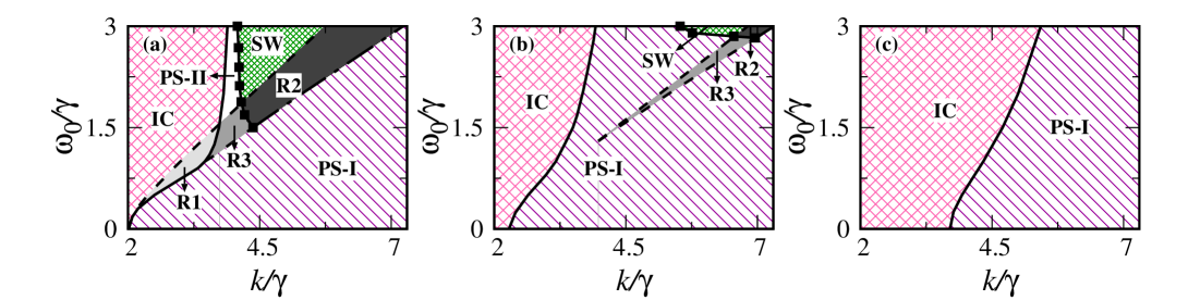
Figure 5: Phase diagrams in the ($k/\gamma-\omega_{0}/\gamma$) plane for $\alpha_{1}~{}=~{}\alpha_{2}=\alpha$. (a) $\alpha=0.1$, (b) $\alpha=0.5$, and (c) $\alpha=1.0$. Bifurcation curves and dynamical states are represented similar to those in Fig. 3. Partially synchronized state II (PS-II) is observed in the region enclosed by pitchfork, Hopf and saddle-node bifurcation curves (see Fig. 5(a)). PS-II and R3 in Fig. 5(b) are enclosed by saddle-node bifurcation curves. Here, R3 corresponds to the region of bistability between IC, and PS-II states.

IV Phase diagrams of the Sakaguchi-Kuramoto model with higher order coupling

In this section, we will proceed to understand the dynamics of the generalized Sagakuchi-Kuramoto model by constructing appropriate two parameter phase diagrams and classifying the underlying states from a numerical analysis of the evolution equations of the macroscopic order parameters Eqs. (16) and (22) corresponding to unimodal and bimodal frequency distributions, respectively. We also solve the associated Sakaguchi-Kuramoto model by numerically integrating Eq. (2) to verify the dynamical transitions in the phase diagrams. Specifically, we will unravel the phase diagrams of the Sakaguchi-Kuramoto model with higher order coupling and unimodal frequency distribution and as well as that with bimodal frequency distribution for various possible combinations of the asymmetry parameters. The number of oscillators is fixed as $N=10^{4}$ and we use the standard fourth-order Runge-Kutta integration scheme with integration step size $h=0.01$ to solve the Sakaguchi-Kuramoto model (2).

IV.1 Unimodal Frequency Distribution

The reduced low-dimensional equations (16), describing the dynamics of the Sakaguchi-Kuramoto model with higher order coupling and unimodal frequency distribution, is characterized by a trivial steady state $(r=0)$, corresponding to the incoherent state (IC) and an oscillatory state corresponding to the standing wave (SW) nature of the Sakaguchi-Kuramoto oscillators. The stability determining eigenvalues of the trivial steady state can be obtained as

$$\lambda_{1,2}=\frac{-2\gamma+k\cos(\alpha_{1})\pm\sqrt{\Delta}}{2},$$ (23)

where $\Delta=k\sin(\alpha_{1})(4\omega_{0}+k\sin(\alpha_{1}))+4\omega_{0}^{2}$. The stability condition/curve for the onset of IC is obtained as

$$k_{HB}=2\gamma\sec(\alpha_{1}).$$ (24)

Phase diagrams of the Sakaguchi-Kuramoto model with higher order coupling and unimodal frequency distribution for different combinations of the asymmetry parameters $\alpha_{1}$ and $\alpha_{2}$ are depicted in Fig. 1. The line connected by filled squares corresponds to the Hopf bifurcation condition (24). In the absence of both the asymmetry parameters, that is for $\alpha_{1}=\alpha_{2}=0$, there is a transition from the incoherent state to the standing wave pattern as a function of $k$ (see Fig. 1(a)) via the Hopf bifurcation curve. Similar dynamical transition is also observed for the other choices of the asymmetry parameters, namely for $\alpha_{1}=\alpha_{2}=1.0$ (see Fig. 1(b)) and for $\alpha_{1}=0$ and $\alpha_{2}=1.0$ (see Fig. 1(d)) except for the region shift. For $\alpha_{1}=1.0$ and $\alpha_{2}=0.0$, one can observe bistability between the IC and SW (indicated by grey shaded region, marked as R1) in Fig. 1(c). The bistable region is bounded by the homoclinic (indicated by dotted-dashed line) and Hopf bifurcation curves. Note that the homoclinic bifurcation curve is obtained from XPPAUT. It is also to be noted that the dynamical transition is independent of $\omega_{0}$ in this case of unimodal frequency distribution, in general.

Now, the time-averaged order paramter $R=\lim_{T\rightarrow\infty}\frac{1}{T}\int_{0}^{T}dt^{\prime}r(t^{\prime})$ estimated from the simulation of the Sakaguchi-Kuramoto model, by numerically integrating Eq. (2), for the unimodal frequency distribution is depicted in Fig. 2 for two different values of the asymmetry parameters. The line connected by open circles corresponds to the forward trace, while the line connected by filled circles corresponds to the backward trace. For $\alpha_{1}=\alpha_{2}=0$, there is a transition from the incoherent state (characterized by the null value of $R$) to the standing wave pattern, corroborated by a finite value of $R$ (seeFig.  2(a)), which is in accordance with the phase diagram in Fig. 1(a) that is obtained from the reduced low-dimensional systems (16). The dotted line is the analytical Hopf bifurcation curve $k_{HB}$ across which there is a transition. Similar dynamical transition will be observed for the other combinations of the asymmetry parameters except for the region shift as in the phase diagrams (see Fig. 1) and hence they are not shown here to avoid repetitions. Nevertheless, there is a bistability between IC and SW as in the phase diagram for $\alpha_{1}=1.0$ and $\alpha_{2}=0.0$ (see 2(b)) bounded by the homoclinic and Hopf bifurcation curves. Thus, direct numerical simulation of the model equation agrees well with the dynamical transitions observed from their reduced low-dimensional equations corresponding to the macroscopic order parameters.

IV.2 Bimodal Frequency Distribution

Case I ($\alpha_{1}=\alpha_{2}$ = 0):

In order to appreciate and understand the effect of the asymmetry parameters $\alpha_{1}$ and $\alpha_{2}$ on the dynamics as represented by the phase diagram, one should first familiarize with the phase diagram of the Sakaguchi-Kuramoto model with higher order coupling and bimodal frequency distribution in the absence of the asymmetry parameters. The phase diagram in the ($\omega_{0}/\gamma$-$k/\gamma$) plane for the case $\alpha_{1}=\alpha_{2}=0$ is depicted in Fig. 3. The dynamical states in the phase diagram are distinguished by features which are essentially based on the asymptotic behavior of $r(t)$. Incoherent state (IC), partially synchronized state (PS-I) and standing wave (SW) along with the bistable regimes (R1 and R2) among the observed dynamical states are depicted in the phase diagram. The parameter space marked as R1 corresponds to the bistable regime between IC and PS-I states, while that indicated as R2 corresponds to the bistable regime between SW and PS-I states. The null value of $r(t)$ characterizes the incoherent state, while a finite value of $r(t)$ indicates partially synchronized states. Oscillating nature of $r(t)$ confirms the standing wave.

The stable regions of the incoherent state in the phase diagram can be inferred from the dynamical equations of the reduced macroscopic variables given in Eqs. (20) and (21). The phases of the oscillators are uniformly distributed between $0$ to $2\pi$ for the incoherent state and hence it is characterized by $z_{1}=z_{2}=0$. Performing a linear stability analysis of the fixed point $(z_{1},~{}z_{2})=(0,~{}0)$, one obtains the condition for stability as

$$k_{PF}=\frac{2(\gamma^{2}+\omega_{0}^{2})}{\gamma},~{}~{}~{}~{}\text{for}~{}\omega_{0}/\gamma~{}~{}<~{}1,$$ (25)

$$k_{HB}=4\gamma~{}~{}~{}~{}~{}~{}~{}~{}~{}\text{for}~{}\omega_{0}/\gamma~{}~{}\geq~{}1.$$ (26)

Here, $K_{PF}$ corresponds to the pitchfork bifurcation curve across which the fixed point $(z_{1},~{}z_{2})=(0,~{}0)$ (incoherent state) loses its stability leading to the inhomogeneous steady state (PS-I state), while $K_{HB}$ corresponds to the Hopf bifurcation curve across which the incoherent state loses its stability resulting in the standing wave pattern. The pitchfork bifurcation curve, indicated by the solid line in Fig. 3, serves as the boundary between the incoherent and partially synchronized state for $\omega_{0}/\gamma~{}~{}<~{}1$. The Hopf bifurcation curve, denoted by the line connected by filled squares, demarcates the incoherent state and standing wave region of the phase diagram. The dashed line in Fig. 3 corresponds to the saddle-node bifurcation curve, while the homoclinic bifurcation curve is denoted as the dotted-dashed line. The latter is obtained from the software XPPAUT xpp , while the former is determined as follows. The inhomogeneous steady state of the PS-I region in the phase diagram is characterized by $r_{1}=r_{2}=r=Const.$ and $\psi_{1}=-\psi_{2}=\phi$, and hence from Eqs. (22) one can obtain

$$\sin(2\phi) =\frac{8\omega_{0}}{k(1+r^{2})(2+r^{2}+r^{2}\cos(2\phi))},$$ (27a)

$$\cos(2\phi) =\frac{k-kr^{2}-a}{(kr^{2}(r^{2}-1))},$$ (27b)

where $a$ =$\sqrt{k^{2}-2k^{2}r^{2}+8k\gamma r^{2}+k^{2}r^{4}-8k\gamma r^{4}}$. The above equations give the following solutions for the stationary $r$ and $\phi$:

$$1 =\frac{64\omega_{0}^{2}(r^{2}-1)^{2}}{(r^{2}+1)^{2}(k-kr^{2}+a)^{2}}+\frac{(kr^{4}-k+a)^{2}}{(k^{2}r^{4}(r^{2}-1)^{2})}$$ (28a)

$$\tan(2\phi) =\frac{8k\omega_{0}r^{2}(r^{2}-1)^{2}}{(r^{2}+1)(k-kr^{2}+a)(kr^{4}-k+a)}.$$ (28b)

Now, one can numerically solve the above equations for fixed values of the parameters to obtain $r$ and $\phi$, which can be substituted back in the original equation of motion of the order parameters, Eqs. (22), to deduce the characteristic eigenvalue equation. The resulting eigenvalues determine the saddle-node bifurcation curves in the ($\omega_{0}/\gamma$-$k/\gamma$) parameter space.

The standing wave pattern loses its stability across the homoclinic bifurcation curve resulting in the PS-I state. Upon decreasing the value of $k/\gamma$ in the phase diagram, the PS-I state (inhomogeneous steady states of $z_{1}$ and $z_{2}$) loses its stability via the saddle-node bifurcation curve resulting in the incoherent state ($z_{1}=z_{2}=0$) up to $\omega_{0}/\gamma=1.6$ and in the standing wave patterns for $\omega_{0}/\gamma>1.6$. Hence, the bistability between the IC and PS-I states is enclosed by the saddle-node and pitchfork bifurcation curves in the phase diagram in the region denoted as R1. Saddle-node and homoclinic bifurcation curves enclose the bistable region between the standing wave and PS-I state, which is denoted as R2 in the phase diagram. It is to be noted that the phase diagram of the Sakaguchi-Kuramoto model with higher order coupling and bimodal frequency distribution in the absence of asymmetry parameters resembles closely that of the Sakaguchi-Kuramoto model with pairwise interactions and bimodal frequency distribution bim . The higher order coupling has essentially enlarged the bistable regions of the phase diagram. Further, the Sakaguchi-Kuramoto model with higher order coupling and bimodal frequency distribution is characterized by PS-I, R1 and R2 when compared to the Sakaguchi-Kuramoto model with higher order coupling and unimodal frequency distribution (compare Figs. 3 and   2(a)). Similar rich dynamical states are also observed for the other choices of the asymmetry parameters in the presence of bimodal frequency distribution as will be elucidated in the following cases.

Now, the order parameter $R$ estimated from the Sakaguchi-Kuramoto model by numerically integrating Eq. (2) for the bimodal frequency distribution is depicted in Fig. 4 for the asymmetry parameters $\alpha_{1}=\alpha_{2}=0$ and for three different values of $\omega_{0}/\gamma$. Here, the line connected by open circles corresponds to the forward trace, while the line connected by filled circles corresponds to the backward trace as in Fig. 2. The dotted vertical line in Fig. 4(a) corresponds to the analytical pitch-fork bifurcation curve, the dotted-dashed line corresponds to the analytical saddle-node bifurcation curve, and the dashed line in Fig. 4(b) corresponds to the analytical Hopf bifurcation curve, while the solid line corresponds to the homoclinic bifurcation curve obtained using XPPAUT. There is a transition from the incoherent state to the standing wave via the pitch-fork bifurcation during the forward trace, whereas there is a transition from the SW to IC via the saddle-node bifurcation during the reverse trace (see Fig. 4(a)) for $\omega_{0}/\gamma=0.75$. Similarly, there is a transition from IC(SW) to SW(IC) via the homoclinic(saddle-node) bifurcation curve during the forward(backward) trace for $\omega_{0}/\gamma=1.5$ as depicted in Fig. 4(b). For $\omega_{0}/\gamma=2.0$, there is a similar transitions via the homoclinic and saddle-node bifurcation curves during the forward and backward traces, respectively. These transitions, obtained by numerically solving the model equation (2), perfectly correlate with the dynamical transitions observed in the phase diagram (see Fig. 3), which are obtained by solving the reduced low-dimensional evolution equations for the macroscopic order parameters (22).

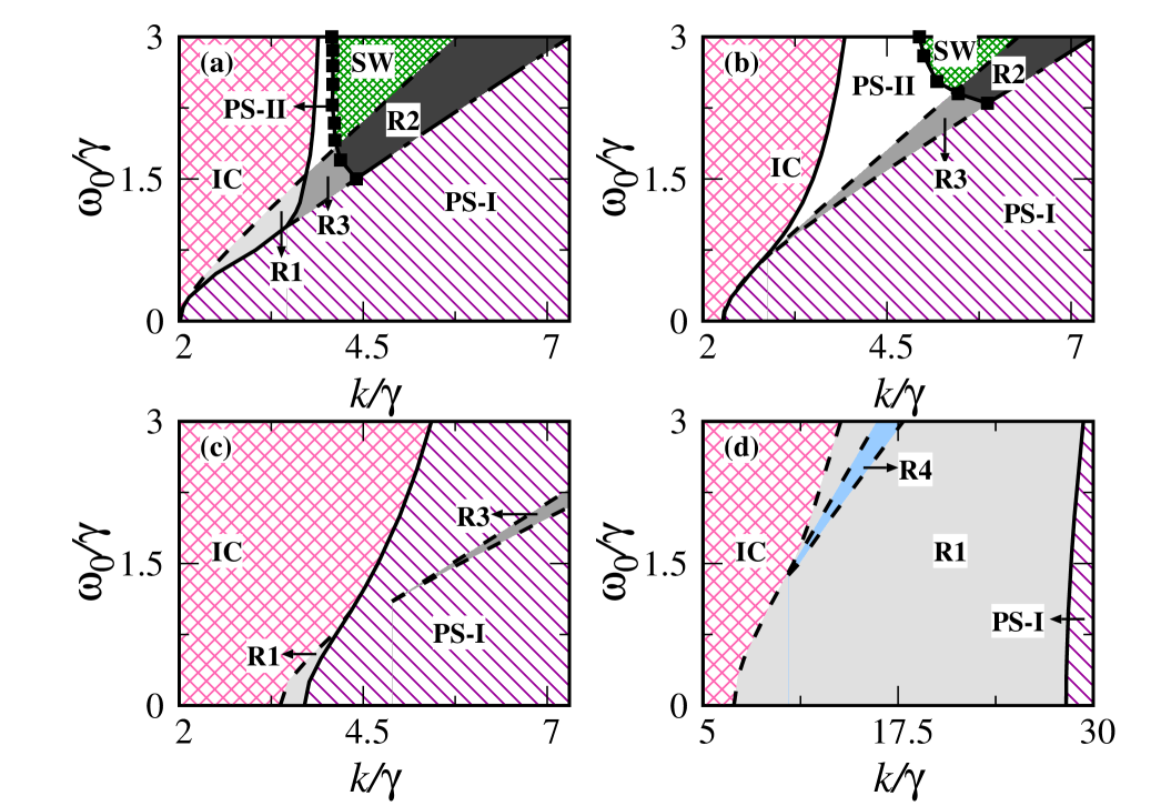
Figure 6: Phase diagrams in the ($k/\gamma-\omega_{0}/\gamma$) plane for $\alpha_{2}~{}=~{}0$ and for various values of the asymmetry parameter in the pairwise coupling. (a) $\alpha_{1}=0.1$, (b) $\alpha_{1}=0.5$, (c) $\alpha_{1}=1.0$ and (d) $\alpha_{1}=1.5$. Bifurcation curves and dynamical states are similar to those in Fig. 5(a). Here, R4 corresponds to the region of multistability between IC, PS-I and PS-II states.

Case II ($\alpha_{1}=\alpha_{2}~{}\neq$ 0):

In order to analyze the effect of the asymmetry parameters on the phase diagram (see Fig. 3), we have next considered the case where the asymmetry parameters $\alpha_{1}~{}=~{}\alpha_{2}~{}=~{}\alpha$ for simplicity. We have depicted the corresponding phase diagrams in the ($k/\gamma-\omega_{0}/\gamma$) plane in Figs. 5(a)-5(c) for $\alpha=0.1,0.5$, and $1$, respectively. The dynamical sates and the bifurcation curves are similar to those in Fig. 3 without any asymmetry parameter. However for $\alpha=0.1$, partially synchronized state-II (PS-II) is characterized by a different set of inhomogeneous steady states corresponding to nonzero values of ($z_{1},~{}z_{2}$) in addition to the dynamical states observed in Fig. 3. A linear stability analysis of the fixed point $(z_{1},~{}z_{2})=(0,~{}0)$ results in the stability condition

$$\omega_{0}^{2}=\frac{{(32\gamma^{3}k+\gamma k^{3})\cos(\alpha_{1})-32\gamma^{4}-6\gamma^{2}k^{2}-4\gamma^{2}k^{2}\cos(2\alpha_{1})}}{{32\gamma^{2}+k^{2}-16\gamma k\cos(\alpha_{1})+k^{2}\cos(2\alpha_{1}])}}.$$ (29)

The above algebraic expression can be further simplified as

$$\gamma k^{3}\cos(\alpha_{1})-32\gamma^{4}-6\gamma^{2}k^{2}+32\gamma^{3}k\cos(\alpha_{1})$$

$$-2\omega_{0}^{2}(k\cos(\alpha_{1})-4\gamma)^{2}-4\gamma^{2}k^{2}\cos(2\alpha_{1})=0,$$ (30)

which actually corresponds to the pitchfork bifurcation curve across which the fixed point $(z_{1},~{}z_{2})=(0,~{}0)$ (incoherent state) loses its stability leading to the partially synchronized states PS-I and PS-II. Note that the incoherent state loses it stability only through the pitchfork bifurcation curve in the entire explored range of $\omega_{0}/\gamma$ (see Fig. 5(a)). All other bifurcation curves are obtained from XPPAUT. One may observe that the PS-II state is enclosed by pitchfork, Hopf and homoclinic bifurcation curves, whereas the region corresponding to the bistability between PS-I and PS-II (denoted by R3) is enclosed by pitchfork, Hopf and saddle-node bifurcation curves. The other dynamical transition and bistable regions are similar to that discussed in Fig. 3 in the absence of the asymmetry parameters. Thus, a rather low value of the asymmetry parameters results in an additional partially synchronized state (PS-II state) with a region of multistability between PS-I and PS-II.

However, a slight increase in the values of the asymmetry parameters results in drastic changes in the phase diagram (see Fig. 5(b) for $\alpha=0.5$). It is evident from the figure that the bistable regions (R2 and R3) and the parameter space with standing wave are reduced drastically with increase in the PS-I state. The PS-II state coexists with the PS-I state in the region enclosed by the two saddle-node bifurcation curves, while the bistable region R1 is completely wiped off from the phase diagram. A large asymmetry parameter results in the loss of bistable regions and standing wave regions completely from the phase diagram, while retaining only the incoherent state and partially synchronized state-I as illustrated in Fig. 5(c) for $\alpha=1$. Further increase in the asymmetry parameter results in similar phase diagrams as in Fig. 5(c).

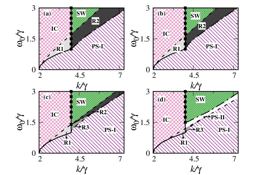
Figure 7: Phase diagrams in the ($k/\gamma-\omega_{0}/\gamma$) plane for $\alpha_{1}~{}=~{}0$ and for various values of the asymmetry parameter in the higher order coupling. (a) $\alpha_{2}=0.1$, (b) $\alpha_{2}=0.5$, (c) $\alpha_{2}=1.0$ and (d) $\alpha_{2}=1.5$. Bifurcation curves and dynamical states are similar to those in Fig. 5(a).

Case III ($\alpha_{1}~{}\neq$  0; $\alpha_{2}$ =  0):

Now, we analyse the nature of the phase diagram with asymmetry parameter only in the pairwise coupling by switching off the asymmetry parameter in the higher order coupling, so that $\alpha_{1}~{}\neq~{}~{}0$ and $\alpha_{2}~{}=~{}~{}0$. The phase diagrams for $\alpha_{1}=0.1,0.5,1$ and $1.5$ are shown in Figs. 6(a)-6(d), respectively. For $\alpha_{1}=0.1$, the dynamics and the dynamical transitions in the phase diagram (see Fig. 6(a)) are similar to those observed in Fig. 5(a) for $\alpha_{1}~{}=~{}\alpha_{2}=0.1$, which elucidates that the onset of PS-II state is facilitated by the asymmetry parameter in the pairwise coupling and is independent of the asymmetry parameter in the higher order coupling. Increasing $\alpha_{1}$ to $\alpha_{1}=0.5$ results in an enhancement of the PS-II state and the bistability between both the partially synchronized states in the phase diagram (see Fig. 6(b)). It is to be noted that R3 is enclosed by the saddle-node and Hopf bifurcation curves. The spread of SW and R2 in the phase diagram is decreased appreciably for increasing values of $\alpha_{1}$, whereas that of PS-I remains almost unaffected. The bistability between the IC and PS-I (region R1) states is completely destroyed.

Next, the phase diagram for $\alpha=1$ is depicted in Fig. 6(c), where the spread of SW and R2 is completely eliminated. Further, the spread of R3 enclosed by the saddle-node bifurcation curves in the phase diagram is considerably reduced. It is to be noted that there is a reemergence of the bistable region R1 even for $\omega_{0}/\gamma~{}<~{}1/\sqrt{3}$, where bimodal frequency distribution becomes unimodal, which elucidates that the bistable region R1 has its manifestation in the phase diagram essentially due to the higher order coupling. Otherwise, the phase diagram is almost equally shared by IC and PS-I states. Further increase in the asymmetry parameter in the pairwise coupling results in the increase in the R1 region to a large extent, where IC and PS-I states coexist and are bounded by the saddle-node and pitchfork bifurcation curves. It is to be noted that a new multistable region enclosed by the saddle-node bifurcation curves appears (denoted as R4 in Fig. 6(d) for $\alpha=1.5$), where IC, PS-I and PS-II states coexist. Thus, it is evident that the asymmetry parameter in the pairwise coupling facilitates several interesting multistable states in the phase diagram mediated by various types of bifurcations.

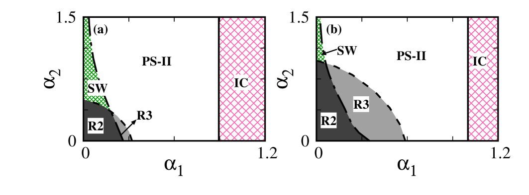
Figure 8: Phase diagrams in the ($\alpha_{1}-\alpha_{2}$) plane for $\omega_{0}/\gamma~{}=~{}2$. (a) $k/\gamma=4.5$, and (b) $k/\gamma=5.0$. Bifurcation curves and dynamical states are similar to those in Fig. 5(a).

Case IV ($\alpha_{2}~{}\neq$  0; $\alpha_{1}$ =  0):

In order to analyze the effect of the asymmetry parameter in higher order interactions alone, we have fixed $\alpha_{1}=0$ and depicted the phase diagrams in Figs. 7(a)-7(d) for $\alpha_{2}=0.1,0.5,1.0$ and $1.5$, respectively. The phase diagram (see Fig. 7(a)) for $\alpha_{2}=0.1$ is similar to the phase diagram in Fig. 3, which is depicted for the choice $\alpha_{1}=\alpha_{2}=0$, but now with an enlarged bistable region R2 enclosed by saddle-node and homoclinic bifurcation curves. Thus, it is again evident that the asymmetry parameters largely contribute to the onset of multistability and facilitate the latter to a large extent. Note that the PS-II state and consequently the region R3 are absent in the phase diagram for $\alpha_{1}=0$, which is actually facilitated by intermediate values of $\alpha_{1}$ (see Figs. 6(a) and  6(b)). Increasing $\alpha_{2}$ to $0.5$ (see Fig. 7(b)), the spread of the bistability region shrinks compared to that in Fig. 7(a). Further increase in the value of the asymmetry parameter in the higher order coupling results in a decrease in the spread of R2 with the onset of R3, where PS-I and PS-II coexist, via the saddle-node bifurcation as depicted in Fig. 7(c) for $\alpha=1.0$. For further larger values of $\alpha_{2}$, the spread of R1 and R3 in the phase diagram decreases to a large extent resulting in the monostable regions of IC, PS-I, PS-II and SW states as depicted in Fig. 7(d) for $\alpha=1.5$. The spread of R2 is completely wiped off from the phase diagram for $\alpha_{2}=1.5$. Thus, it is evident that large values of $\alpha_{2}$ facilitate the onset of PS-II and eventually R3, while smaller values of $\alpha_{2}$ favor the spread of bistable regions to a large extent.

Case V ($\alpha_{1}~{}>0~{}\&~{}\alpha_{2}>0$):

Now, we consider $\alpha_{1}>0$ and $\alpha_{2}>0$ in order to analyze the dynamical states and their transitions due to the trade-off between the asymmetry parameters in both pair-wise and higher order couplings. Phase diagrams in the asymmetry parameter ($\alpha_{1},\alpha_{2}$) space for $\omega_{0}/\gamma=2$ and for two different values of $k/\gamma$ are depicted in Figs. 8. The dynamical states and their bifurcation transitions are found to be similar to those in the previous figures. For low values of $\alpha_{2}$, there is a transition from R2 to R3 via the homoclinic bifurcation and then to PS-II state via the saddle-node bifurcation and finally to IC state through the pitchfork bifurcation as a function of $\alpha_{1}$. For larger values of $\alpha_{2}$, there is a transition from SW to PS-II via the homoclinic bifurcation and then to IC via the pitchfork bifurcation as a function of $\alpha_{1}$. Small to intermediate values of $\alpha_{1}$ and $\alpha_{2}$ favor bistable states R2 and R3, while larger values of the asymmetry parameters $\alpha_{1}$ and/or $\alpha_{2}$ result in monostable states (see Figs. 8 and  5). Increasing $k/\gamma$ from $4.5$ to $5$ results in increase in the spread of bistable regions R2 and R3 (compare Figs. 8(a) and  8(b) ).

V Summary and Conclusion

Higher order interactions have physical relevance in physics and neuroscience and they have gained recent interest in network theory. In this work, we have investigated the phase diagrams of the Sakaguchi-Kuramoto model along with a higher order interaction, and unimodal and bimodal distributions of the natural frequencies of the individual phase oscillators. We have also introduced asymmetry parameters both in the pairwise and higher order couplings to elucidate their role in the dynamical transitions in the phase diagram. We have investigated the effects of five possible combinations of the asymmetry parameters $\alpha_{1}$ and $\alpha_{2}$ on the phase diagram along with the higher order interaction. Using the Ott-Antonsen ansatz, we have obtained the coupled evolution equations corresponding to the macroscopic order parameters. We have deduced the analytical stability condition for the linear stability of the incoherent state, resulting in the pitchfork bifurcation curve, using the governing equations of the macroscopic order parameters. Further, we have also analytically deduced the Hopf bifurcation curve for $\alpha_{1}=0$, while the saddle-node and homoclinic bifurcation curves are obtained using the software package XPPAUT. The Sakaguchi-Kuramoto model along with a higher order interaction and unimodal frequency distribution displays only IC and SW states, and bistability among them for $\alpha_{1}=1.0$ and $\alpha_{2}=0.0$. In contrast, we have observed rich phase diagrams with dynamical states such as IC, PS-I, PS-II and SW states along with the bistable (R1, R2 and R3) and multistable (R4) states with the bimodal frequency distribution.

In the absence of asymmetry parameters, higher order couplings favor the spread of the bistable states R1 and R2 to a large extent when compared to the Sakaguchi-Kuramoto model with pairwise coupling alone and bimodal frequency distribution. Further, the asymmetry parameters favor the onset of the bistable regions R3 and R4 which are generally absent in the Sakaguchi-Kuramoto model with pairwise coupling and bimodal frequency distribution. It is to be noted that rather low values of the asymmetry parameter in the pairwise coupling for $\alpha_{2}=0$ and relatively larger values of the asymmetry parameter in the higher order coupling for $\alpha_{1}=0$ favors the onset of PS-II state and eventually the region R3 in the phase diagrams. However, very large values of both the asymmetry parameters render the phase diagram only with monostable dynamical states. It is to be noted that there exists bistable region R1 even for $\omega_{0}/\gamma~{}<~{}1/\sqrt{3}$ in the phase diagrams, where the bimodal frequency distribution breaks down to unimodal one, which is purely a manifestation of the higher order coupling as the bistable region R1, which has not yet been observed in the Sakaguchi-Kuramoto model with pairwise coupling only along with unimodal frequency distribution. We sincerely believe that the above results, with rich phase diagrams comprising of bistable and monostable regions of the Sakaguchi-Kuramoto model due to the tradeoff between the asymmetry parameters and the higher order coupling, provide valuable new insights on the dynamical nature of the model. Note that the presence of bistable (multistable) regions denote the regions across which abrupt dynamical transition occurs, a typical nature of biological systems and, in particular, in neuroscience where bistability and fast switching between states are very relevant.

References

- (1) Y. Kuramoto, Chemical Oscillations, Waves and Turbulence (Springer, 1984).
- (2) A.T. Winfree, ”Biological rhythms and the behavior of populations of coupled oscillators”, J. Theor. Biol. 16, 15 (1967).
- (3) S. H. Strogatz, ”From Kuramoto to Crawford: exploring the onset of synchronization in populations of coupled oscillators”, Physica D 143, 1 (2000).
- (4) A. Pikovsky, M. Rosenblum and J. Kurths,Synchronization: a Universal Concept in Nonlinear Sciences (Cambridge University Press, Cambridge, 2001).
- (5) A. J. Acebron, J. J. Bonilla, C. J. P. Vicente, F. Ritort and R. Spigler, ”The Kuramoto model: a simple paradigm for synchronization phenomena”, Rev. Mod. Phys.77, 137 (2005).
- (6) S. Gupta, A. Campa and S. Ruffo, ”Kuramoto model of synchronization: equilibrium and nonequilibrium aspects”, J. Stat. Mech. 8 R08001 (2014).
- (7) S. Gupta, A. Campa and S. Ruffo, Statistical Physics of Synchronization (Springer, Berlin, 2018).
- (8) C. S. Peskin, ”Mathematical aspects of heart physiology”,(Courant Institute of Mathematical Sciences, New York 1975).
- (9) J. Buck, ”Synchronous rhythmic flashing of fireflies. II.”, Q. Rev. Biol. 63, 265 (1988).
- (10) T. J. Walker, ”Acoustic synchrony: two mechanisms in the snowy tree cricket”, Science 166, 891 (1969).
- (11) I. Kiss, Y. Zhai and J. Hudson ”Emerging coherence in a population of chemical oscillators”, Science 296, 1676 (2002).
- (12) R. Schmidt, K. J. R LaFleur and M. A. de Reus, ”Kuramoto model simulation of neural hubs and dynamic synchrony in the human cerebral connectome”, BMC Neurosci. 16, 54 (2015).
- (13) Z. Néda, E. Ravasz, T. Vicsek, Y. Brechet and A. L. Barabási, ”Physics of the rhythmic applause”, Phys. Rev. E 61, 6987 (2000).
- (14) D. Iatsenko, S. Petkoski, P. V. E. McClintock and A. Stefanovska,”Stationary and traveling wave states of the Kuramoto model with an arbitrary distribution of frequencies and coupling strengths”, Phys. Rev. Lett. 110, 064101 (2013).
- (15) S. Petkoski, D. Iatsenko, L. Basnarkov and A. Stefanovska, ”Mean-field and mean-ensemble frequencies of a system of coupled oscillators”, Phys. Rev. E 87, 032908 (2013).
- (16) D. Iatsenko, P.V.E. McClintock and A. Stefanovska, ”Glassy states and super-relaxation in populations of coupled phase oscillators, Nature Communications 5, 4118 (2014).
- (17) C. Gu, X. Liang, . Yang and J. H. T. Rohling, ”Heterogeneity induces rhythms of weakly coupled circadian neurons, Sci. Rep. 6, 21412 (2016).
- (18) Y. Seong-Gyu, H. Hong and B. J. Kim,”Asymmetric dynamic interaction shifts synchronized frequency of coupled oscillators”, Sci. Rep. 10, 2516 (2020).
- (19) H. Sakaguchi, Y. Kuramoto, S. Shinomoto, ”Mutual entrainment in oscillator lattices with N on variational type interaction ”, Prog. Theor. Phys. 79, 5 (1988).
- (20) O. M. Omel’chenko, and M. Wolfrum, ”Nonuniversal transitions to synchrony in the Sakaguchi-Kuramoto model”, Phys. Rev. Lett. 109, 164101 (2012).
- (21) O. M. Omel’chenko, and M. Wolfrum, ”Bifurcations in the Sakaguchi-Kuramoto model”, Physica D 74, 263 (2013).
- (22) H. Sakaguchi and Y. Kuramoto, ”A Soluble active rotator model showing phase transitions via mutual entrainment”, Prog. Theor. Phys. 76, 576 (1986).
- (23) K. Wiesenfeld, P. Colet and S. H. Strogatz, ”Synchronization transitions in a disordered Josephson series array”, Phys. Rev. Lett. 76, 404 (1996).
- (24) Anil Kumar and J. Sarika,”Explosive synchronization in interlayer phase-shifted Kuramoto oscillators on multiplex networks”, Chaos, 3, 041103 (2021).
- (25) J. Sarika, K. Ajay Deep, and J. Hawoong, ”Explosive synchronization in multilayer dynamically dissimilar networks”, Journal of Computa. Sci., 26, 101177 (2020).
- (26) J. Sarika, K. Anil and L. Inmaculada, ”Explosive synchronization in frequency displaced multiplex networks”, Chaos, 29, 041102 (2019).
- (27) K. Anil, J. Sarikaa nd K. Ajay Deep, ”Interlayer adaptation-induced explosive synchronization in multiplex networks”, Phy. Rev. R, 2, 023259 (2020).
- (28) M. K. Stephen Yeung and S. H. Strogatz, ”Time delay in the Kuramoto model of coupled oscillators”, Phys. Rev. Lett. 82, 648 (1999).
- (29) A. Pikovsky and M. Rosenblum, ”Partially integrable dynamics of hierarchical populations of coupled oscillators”, Phys. Rev. Lett. 101, 264103 (2008).
- (30) M. Wolfrum, and O. E. Omel’chenko, ”Chimera states are chaotic transients”, Phys. Rev. E 84, 015201(R) (2011).
- (31) D. Pazó and D. Montbrió, ”Low-dimensional dynamics of populations of pulse-coupled oscillators”, Phys. Rev. X 4, 011009 (2014).
- (32) I. Iacopini, G. Petri, A. Barrat and V. Latora, ”Simplicial models of social contagion” Nat. Commun. 10, 2485 (2019).
- (33) J. T. Matamalas, S. Gómez, and A. Arenas, ”Abrupt phase transition of epidemic spreading in simplicial complexes”, Phys. Rev. Res. 2, 012049(R) (2019).
- (34) R. Mulas, C. Kuehn and J. Jost, ”Coupled dynamics on hypergraphs: master stability of steady states and synchronization”, Phys. Rev. E 101, 062313 (2020).
- (35) M. Lucas, G. Cencetti and F. Battiston, ” Multiorder Laplacian for synchronization in higher order networks”, Phys. Rev. Res. 2, 033410 (2020).
- (36) W. Huobin, H. Wenchen and Y. Junzhong, ”Synchronous dynamics in the Kuramoto model with biharmonic interaction and bimodal frequency distribution”, Phys. Rev. E 96, 022202 (2017).
- (37) Ch. Bick, M. Timme, D. Paulikat, D. Rathlev and P. Ashwin, ”Chaos in symmetric phase oscillator networks, Phys. Rev. Lett., 107, 244101 (2011).
- (38) Ch. Bick, P. Ashwin, and A. Rodrigues, ”Chaos in generically coupled phase oscillator networks with non-pairwise interactions”, Chaos, 26, 094814 (2016).
- (39) X. Can, X. Hairong, G. Jian and Z. Zhigang, ”Collective dynamics of identical phase oscillators with high-order coupling”, Sci. Rep., 6, 31133 (2016).
- (40) P. S. Skardal and A. Arenas ”Higher order interactions in complex networks of phase oscillators promote abrupt synchronization switching”, Commun. Phys. 3, 218 (2020).
- (41) V. Salnikov, D. Cassese and R. Lambiotte, ”Simplicial complexes and complex systems” Eur. J. Phys. 40, 014001 (2019).
- (42) O. T. Courney and G. Bianconi, ”Generalized network structures: The configuration model and the canonical ensemble of simplicial complexes” Phys. Rev. E 93, 062311 (2016).
- (43) G. Bianconi and C. Rahmede, ”Emergent hyperbolic network geometry” Sc. Reports 7, 41974 (2017).
- (44) T. Fellin, O Pascual, S Gobbo, T Pozzan and P G Haydon, ”Neuronal synchrony mediated by astrocytic glutamate through activation of extrasynaptic NMDA receptors” Neuron 43, 729–743 (2004).
- (45) A. Tlaie, I. Leyva and I. Sendiña-Nadal,” High-order couplings in geometric complex networks of neurons” Phys. Rev. E 100, 052305 (2019).
- (46) N.J. Allen and B. A. Barres, ”Glia-more than just brain glue” Nature 457, 675–677 (2009).
- (47) A. Tlaie, I. Leyva and I. Sendiña-Nadal, ”High-order couplings in geometric complex networks of neurons” Phys. Rev. E 100, 052305 (2019).
- (48) E. Ott, and T. M. Antonsen, ”Low dimensional behavior of large systems of globally coupled oscillators”, Chaos 18, 037113 (2008).
- (49) E. Ott and T. M. Antonsen, ”Long time evolution of phase oscillator systems”, Chaos 19, 023117 (2009).
- (50) B. Ermentrout,Simulating, analyzing, and animating dynamical systems: A guide to XPPAUT for researchers and students, (Society for Industrial & Applied Math, Philadelphia, PA, 2002).
- (51) E. A. Martens, E. Barreto, S. H. Strogatz, E. Ott, P. So and T. M. Antonsen ”Exact results for the Kuramoto model with a bimodal frequency distribution ”, Phys. Rev. E 79, 026204 (2009).