Influence of Charge on Extended Decoupled Anisotropic Solutions in $f(\mathcal{R},\mathcal{T},\mathcal{R}_{\lambda\xi}\mathcal{T}^{\lambda\xi})$ Gravity

Abstract

In this paper, we consider static self-gravitating spherical spacetime and determine various anisotropic solutions through the extended gravitational decoupling technique in $f(\mathcal{R},\mathcal{T},\mathcal{R}_{\lambda\xi}\mathcal{T}^{\lambda\xi})$ gravity to analyze the influence of electromagnetic field on them. We construct two different sets of modified field equations by employing the transformations on both radial as well as temporal metric potentials. The first set symbolizes the isotropic fluid distribution, thus we take Krori-Barua solution to deal with it. The indefinite second sector comprises the influence of anisotropy. In this regard, we apply some constraints to determine unknowns. Further, we observe the impact of charge as well as decoupling parameter $\zeta$ on the developed physical variables (such as energy density, radial and tangential pressures) and anisotropy. We also analyze other physical features of the compact geometry like mass, compactness and redshift along with the energy conditions. Eventually, we find that our both solutions show less stable behavior for higher values of charge near the boundary in this gravity.

Keywords: $f(\mathcal{R},\mathcal{T},\mathcal{R}_{\lambda\xi}\mathcal{T}^{\lambda\xi})$ gravity; Anisotropy; Gravitational decoupling; Self-gravitating systems.
PACS: 04.50.Kd ; 04.40.Dg; 04.40.-b.

1 Introduction

The composition of our universe is well-structured yet inscrutable, comprising of heavily geometrical objects like stars, galaxies and other unfathomable ingredients. The study of physical features of such massive structures plays an important role to figure out cosmic evolution. Einstein developed first General Relativity (GR) which allows scientists to get better understanding of both cosmological as well as astrophysical phenomena. Several cosmological experiments have been performed on the distant galaxies which indicate that our universe is in the state of accelerating expansion. This expansion is thought to be executed by the dark energy which is repulsive in nature. The modifications to GR have therefore been identified highly significant to reveal mysterious characteristics of our cosmos. The simplest modification to GR is obtained by replacing the Ricci scalar $\mathcal{R}$ with its generic function in an Einstein-Hilbert action, named as $f(\mathcal{R})$ theory. Numerous research [1]-[4] has been done in this theory to analyze the physical feasibility of compact structures through different techniques. The Lané-Emden equation in $f(\mathcal{R})$ theory has been employed by Capozziello et al. [5] to discuss the stability of various mathematical models. Many authors [6]-[13] studied different astronomical objects and examined their formation as well as stable configuration.

Initially, the concept of matter-geometry coupling was introduced by Bertolami et al. [14]. They studied the effects of coupling in $f(\mathcal{R})$ gravity by taking the Lagrangian as a function of $\mathcal{R}$ and $\mathcal{L}_{m}$. This kind of interaction in modified theories has prompted many researchers to put their concentration on accelerating nature of cosmic expansion. Many other modified theories have been developed in the last decade to investigate the role of arbitrary matter-geometry interaction on massive structures, one of them is the $f(\mathcal{R},\mathcal{T})$ theory introduced by Harko et al. [15] in which $\mathcal{T}$ expresses trace of the stress-energy tensor. Such interaction provides the non-conserved energy-momentum tensor which may lead to the accelerated expansion of universe. Later, another theory involving more complex functional was presented by Haghani et al. [16], named as $f(\mathcal{R},\mathcal{T},\mathcal{Q})$ gravity, where $\mathcal{Q}\equiv\mathcal{R}_{\lambda\xi}\mathcal{T}^{\lambda\xi}$. The conserved equations of motion have also been found through Lagrange multiplier approach in this theory. In this scenario, Sharif and Zubair assumed some mathematical models in FRW spacetime and figured out the black hole laws of thermodynamics [17] as well as energy bounds [18].

The development of this modified gravity was premised on the insertion of the factor $\mathcal{Q}$ which ensures the presence of strong non-minimal matter-geometry coupling in self-gravitating systems. The modification in the Einstein-Hilbert action may help in explaining the role of dark energy and dark matter, without resorting to exotic fluid distribution. Some other extensions to GR like $f(\mathcal{R},\mathcal{L}_{m})$ and $f(\mathcal{R},\mathcal{T})$ gravitational theories also comprise the matter Lagrangian involving such arbitrary interaction but we cannot consider their functionals as the most generalized form that provide proper understanding to the influence of coupling on self-gravitating objects in some scenarios. It must be noted here that the factor $\mathcal{R}_{\lambda\xi}\mathcal{T}^{\lambda\xi}$ could explain the impact of non-minimal interaction in the situation where $f(\mathcal{R},\mathcal{T})$ theory breaks down to achieve such results. In particular, $f(\mathcal{R},\mathcal{T})$ theory does not provide coupling effects on the gravitational model for the case when trace-free energy-momentum tensor (i.e., $\mathcal{T}=0$) is considered, however, this phenomenon can be explained by $f(\mathcal{R},\mathcal{T},\mathcal{Q})$ gravity. Due to the non-conservation of energy-momentum tensor in this theory, an additional force is present due to which the motion of test particles in geodesic path comes to an end. This force also helps to elucidate the galactic rotation curves.

Haghani et al. [16] considered three different models such as $\mathcal{R}+\varrho\mathcal{Q},~{}\mathcal{R}(1+\varrho\mathcal{Q})$ and $\mathcal{R}+\gamma\sqrt{\mid\mathcal{T}\mid}+\varrho\mathcal{Q}$ in this framework and discussed their cosmological applications, where $\varrho$ and $\gamma$ are arbitrary coupling constants. The dynamics and cosmic evolution has been explored with respect to these models with and without considering the energy conservation. Odintsov and Sáez-Gómez [19] studied various models in $f(\mathcal{R},\mathcal{T},\mathcal{Q})$ theory and solved their corresponding gravitational equations through numerical methods. They also highlighted some serious issues linked with the matter instability. Ayuso et al. [20] obtained the conditions for different compact objects to be stable in this theory by considering some suitable scalar and vector fields. They concluded that the existence of matter instability is necessary for the case of vector field. For FRW geometry, Baffou et al. [21] incorporated the perturbation functions to calculate the solution of modified field equations and checked their viability. Yousaf et al. [22]-[27] studied the evolution of charged/uncharged spherical as well as cylindrical geometries with the help of effective structure scalars.

The existence of electromagnetic field in celestial structures helps to understand their expansion and stability in a better way. Numerous investigations have been performed in GR as well as modified theories to analyze the role of charge on different physical properties of celestial objects. The Einstein field equations coupled with the charge are known as Einstein-Maxwell equations whose solution has been found by Das et al. [28] through matching the static interior spacetime with exterior Reissner-Nordström. Sunzu et al. [29] examined the quark stars influenced from charge by utilizing the mass-radius relation. Murad [30] analyzed the charged strange stars having anisotropic configuration and studied its physical characteristics. Many authors [31]-[38] analyzed different stellar structures and observed their more stable behavior due to the presence of charge.

The nature of field equations corresponding to the self-gravitating body is highly non-linear, thus it is much difficult task to obtain their exact solution. There has been various techniques to solve these equations in the literature corresponding to the celestial objects coupled with isotropic as well as anisotropic configurations. Sharif and Waseem [39, 40] investigated the viability and stability of several compact objects in curvature-matter coupled gravity by using Krori-Barua ansatz. They found that solutions for anisotropic matter distribution are stable, while isotropic configured stars are shown to be unstable near the core. Maurya et al. [41] considered the minimal coupling model as $f(\mathcal{R},\mathcal{T})=\mathcal{R}+2\chi\mathcal{T}$ ($\chi$ is served as the coupling parameter) and examined the physical viability of anisotropic structures through embedding class one condition along with MIT bag model. Several compact anisotropic configurations have been discussed by Shamir and Fayyaz [42] in $f(\mathcal{R})$ theory by taking different models. The newly developed method, namely minimal geometric deformation (MGD) by means of gravitational decoupling has been found to be significant to develop physically feasible solutions in the field of cosmology and astrophysics. This technique was initially introduced by Ovalle [43] in the braneworld scenario to develop exact solutions for spherical interstellar structures. The formulation of analytical solutions for isotropic geometry has been done by Ovalle and Linares [44] in the context of braneworld. They also shown their compatibility with the Tolman IV solution. Casadio et al. [45] calculated a new solution for spherical exterior geometry which shows singular behavior at Schwarzschild radius.

Ovalle [46] utilized the decoupling scheme to obtain anisotropic exact solution for a compact sphere. Ovalle et al. [47] considered the isotropic solution and extended it to various anisotropic solutions whose feasibility has been analyzed graphically. Gabbanelli et al. [48] formulated physically acceptable anisotropic solution by assuming Duragpal-Fuloria isotropic ansatz. Estrada and Tello-Ortiz [49] considered Heintzmann solution for isotropic distribution and found different physically viable anisotropic solutions. Sharif and Sadiq [50] employed Krori-Barua anstaz and determined two anisotropic solutions through this method. They also analyzed the influence of decoupling parameter and charge on physical parameters as well as energy bounds. Sharif and his collaborators [51]-[54] generalized different anisotropic solutions to modified theories such as $f(\mathcal{G})$ and $f(\mathcal{R})$, where $\mathcal{G}$ represents the Gauss-Bonnet invariant. Singh et al. [55] utilized class one condition to obtain various anisotropic solutions with the help of same strategy. Hensh and Stuchlík [56] constructed different feasible anisotropic solutions by employing a suitable deformation function on the field equations along with Tolman VII solution.

Although the MGD technique (in which the radial metric component is transformed only, while the temporal component remains preserved) is an immensely valuable approach to find exact feasible solutions of the complicated field equations. This is nevertheless possible only if energy is not exchanged from one source to another. Ovalle [57] addressed this issue by proposing a novel strategy, named as extended gravitational decoupling (EGD). This technique transforms both (radial and temporal) metric potentials and also works for any choice of fluid distribution for all spacetime regions. Through this scheme, Contreras and Bargueño [58] presumed vacuum BTZ solution corresponding to the $2+1$-dimensional geometry and found its extension for the charged case. Sharif and Ama-Tul-Mughani have employed this method along with the isotropic Tolman IV [59] as well as charged Krori-Barua [60] anstaz and constructed various anisotropic solutions. Sharif and Saba [61] calculated anisotropic spherical solutions by considering Tolman IV in $f(\mathcal{G})$ gravity. We have recently checked the physical feasibility of two charged/uncharged anisotropic solutions obtained through MGD approach in $f(\mathcal{R},\mathcal{T},\mathcal{Q})$ theory [62, 63]. Sharif and Majid [64]-[66] formulated various cosmological solutions by extending the isotropic Krori-Barua and Tolman IV solutions with the help of MGD as well as EGD techniques in the framework of Brans-Dicke gravity.

This paper examines the effects of charge on various anisotropic solutions constructed through EGD technique in $f(\mathcal{R},\mathcal{T},\mathcal{Q})$ scenario. The paper has the following structure. In the next section, we shall present some fundamental terminologies of this modified theory. Section 3 discusses the EGD technique which helps to split the field equations into two independent sets by deforming the radial as well as temporal metric components. We assume the Krori-Barua solution in section 4 and employ some additional constraints to formulate two anisotropic solutions. We also discuss their viability and stability by means of graphs. Lastly, we sum up our results in section 5.

2 The $f(\mathcal{R},\mathcal{T},\mathcal{Q})$ Gravity

The modified Einstein-Hilbert action (with $\kappa=8\pi$) influenced by an additional source is given as [19]

$$S_{f(\mathcal{R},\mathcal{T},\mathcal{R}_{\lambda\xi}\mathcal{T}^{\lambda\xi})}=\int\left[\frac{f(\mathcal{R},\mathcal{T},\mathcal{R}_{\lambda\xi}\mathcal{T}^{\lambda\xi})}{16\pi}+\mathcal{L}_{m}+\mathcal{L}_{\mathcal{E}}+\zeta\mathcal{L}_{\Upsilon}\right]\sqrt{-g}d^{4}x,$$ (1)

where $\mathcal{L}_{m},~{}\mathcal{L}_{\mathcal{E}}$ and $\mathcal{L}_{\Upsilon}$ indicate the Lagrangian densities of matter configuration, electromagnetic field and new gravitationally coupled source, respectively. In this case, we take $\mathcal{L}_{m}=-\mu$, $\mu$ is the energy density of the fluid. The field equations analogous to the action (1) have the form as

$$\mathcal{G}_{\lambda\xi}=8\pi\mathcal{T}_{\lambda\xi}^{(tot)}.$$ (2)

The geometry of the celestial structure is expressed by an Einstein tensor $\mathcal{G}_{\lambda\xi}$ whereas $\mathcal{T}_{\lambda\xi}^{(tot)}$ is the energy-momentum tensor including all sources. We further write it as

$$\mathcal{T}_{\lambda\xi}^{(tot)}=\mathcal{T}_{\lambda\xi}^{(eff)}+\zeta\Upsilon_{\lambda\xi}=-\frac{1}{\mathcal{L}_{m}f_{\mathcal{Q}}-f_{\mathcal{R}}}\left(\mathcal{T}_{\lambda\xi}^{(m)}+\mathcal{E}_{\lambda\xi}\right)+\mathcal{T}_{\lambda\xi}^{(\mathcal{D})}+\zeta\Upsilon_{\lambda\xi}.$$ (3)

The presence of new source $\Upsilon_{\lambda\xi}$ via certain scalar, vector or tensor field generates anisotropy in the self-gravitating body. The decoupling parameter $\zeta$ measures how much that source affects the geometry. In addition, the quantity $\mathcal{T}_{\lambda\xi}^{(eff)}$ can be viewed as the stress-energy tensor in $f(\mathcal{R},\mathcal{T},\mathcal{Q})$ gravity which comprises the usual physical variables as well as modified correction terms. In this scenario, the modified sector $\mathcal{T}_{\lambda\xi}^{(D)}$ takes the form

$$\mathcal{T}_{\lambda\xi}^{(\mathcal{D})} = -\frac{1}{8\pi\big{(}\mathcal{L}_{m}f_{\mathcal{Q}}-f_{\mathcal{R}}\big{)}}\left[\left(f_{\mathcal{T}}+\frac{1}{2}\mathcal{R}f_{\mathcal{Q}}\right)\mathcal{T}_{\lambda\xi}^{(m)}+\left\{\frac{\mathcal{R}}{2}(\frac{f}{\mathcal{R}}-f_{\mathcal{R}})-\mathcal{L}_{m}f_{\mathcal{T}}\right.\right.$$ (4)

$$- \left.\frac{1}{2}\nabla_{\rho}\nabla_{\eta}(f_{\mathcal{Q}}\mathcal{T}^{\rho\eta})\right\}g_{\lambda\xi}-\frac{1}{2}\Box(f_{\mathcal{Q}}\mathcal{T}_{\lambda\xi})-(g_{\lambda\xi}\Box-\nabla_{\lambda}\nabla_{\xi})f_{\mathcal{R}}$$

$$- 2f_{\mathcal{Q}}\mathcal{R}_{\rho(\lambda}\mathcal{T}_{\xi)}^{\rho}+\nabla_{\rho}\nabla_{(\lambda}[\mathcal{T}_{\xi)}^{\rho}f_{\mathcal{Q}}]+2(f_{\mathcal{Q}}\mathcal{R}^{\rho\eta}+\left.f_{\mathcal{T}}g^{\rho\eta})\frac{\partial^{2}\mathcal{L}_{m}}{\partial g^{\lambda\xi}\partial g^{\rho\eta}}\right],$$

where $f_{\mathcal{R}},~{}f_{\mathcal{T}}$ and $f_{\mathcal{Q}}$ show the derivatives of functional $f(\mathcal{R},\mathcal{T},\mathcal{Q})$ with respect to their subscripts. Moreover, $\nabla_{\xi}$ indicates the covariant derivative and $\Box\equiv g^{\lambda\xi}\nabla_{\lambda}\nabla_{\xi}$.

The stress-energy tensor for perfect matter is given as

$$\mathcal{T}_{\lambda\xi}^{(m)}=(\mu+p)\mathcal{K}_{\lambda}\mathcal{K}_{\xi}+pg_{\lambda\xi},$$ (5)

where $p$ indicates the isotropic pressure and $\mathcal{K}_{\lambda}$ is the four-velocity. The following equation provides the trace of $f(\mathcal{R},\mathcal{T},\mathcal{Q})$ field equations as

$$3\nabla^{\xi}\nabla_{\xi}f_{\mathcal{R}}+\mathcal{R}\left(f_{\mathcal{R}}-\frac{\mathcal{T}}{2}f_{\mathcal{Q}}\right)-\mathcal{T}(f_{\mathcal{T}}+1)+\frac{1}{2}\nabla^{\xi}\nabla_{\xi}(f_{\mathcal{Q}}\mathcal{T})+\nabla_{\lambda}\nabla_{\xi}(f_{\mathcal{Q}}\mathcal{T}^{\lambda\xi})$$

$$-2f+(\mathcal{R}f_{\mathcal{Q}}+4f_{\mathcal{T}})\mathcal{L}_{m}+2\mathcal{R}_{\lambda\xi}\mathcal{T}^{\lambda\xi}f_{\mathcal{Q}}-2g^{\rho\eta}\frac{\partial^{2}\mathcal{L}_{m}}{\partial g^{\rho\eta}\partial g^{\lambda\xi}}\left(f_{\mathcal{T}}g^{\lambda\xi}+f_{\mathcal{Q}}R^{\lambda\xi}\right)=0.$$

The assumption $\mathcal{Q}=0$ in the above equation vanishes strong matter-geometry interaction in a self-gravitating object and provides $f(\mathcal{R},\mathcal{T})$ theory, whereas one can retrieve $f(\mathcal{R})$ theory by considering vacuum scenario. The electromagnetic energy-momentum tensor takes the form

$$\mathcal{E}_{\lambda\xi}=-\frac{1}{4\pi}\left[\frac{1}{4}g_{\lambda\xi}\mathcal{F}^{\rho\eta}\mathcal{F}_{\rho\eta}-\mathcal{F}^{\eta}_{\lambda}\mathcal{F}_{\xi\eta}\right],$$

where the Maxwell field tensor is defined as $\mathcal{F}_{\lambda\xi}=\omega_{\xi;\lambda}-\omega_{\lambda;\xi}$, in which $\omega_{\xi}=\omega(r)\delta_{\xi}^{0}$ is the four potential. This tensor must satisfy the following equations

$$\mathcal{F}^{\lambda\xi}_{;\xi}=4\pi\mathcal{J}^{\lambda},\quad\mathcal{F}_{[\lambda\xi;\eta]}=0.$$

The current density $\mathcal{J}^{\lambda}$ can be expressed as $\mathcal{J}^{\lambda}=\varrho\mathcal{K}^{\lambda}$, where $\varrho$ is the charge density.

We consider a geometry which is separated into two regions, namely interior and exterior at the hypersurface $\Sigma$. The static spherically symmetric astrophysical structure is expressed by the metric as follows

$$ds^{2}=-e^{\chi}dt^{2}+e^{\beta}dr^{2}+r^{2}d\theta^{2}+r^{2}\sin^{2}\theta d\varphi^{2},$$ (6)

where $\chi=\chi(r)$ and $\beta=\beta(r)$. The above metric produces the Maxwell field equations as

$$\omega^{\prime\prime}+\frac{1}{2r}\big{[}4-r(\chi^{\prime}+\beta^{\prime})\big{]}\omega^{\prime}=4\pi\varrho e^{\frac{\chi}{2}+\beta},$$ (7)

which after integration produces

$$\omega^{\prime}=\frac{q}{r^{2}}e^{\frac{\chi+\beta}{2}},$$ (8)

where $q$ shows the charge in the interior geometry (6). Here, ${}^{\prime}=\frac{\partial}{\partial r}$. The four-velocity involves single non-zero component due to the consideration of comoving framework. Thus, it has the form

$$\mathcal{K}^{\xi}=(e^{\frac{-\chi}{2}},0,0,0).$$ (9)

We establish the field equations in $f(\mathcal{R},\mathcal{T},\mathcal{Q})$ theory corresponding to sphere (6) as

$$8\pi\left(\tilde{\mu}+\frac{s^{2}}{8\pi r^{4}}-\mathcal{T}_{0}^{0(\mathcal{D})}-\zeta\Upsilon_{0}^{0}\right) =e^{-\beta}\left(\frac{\beta^{\prime}}{r}-\frac{1}{r^{2}}\right)+\frac{1}{r^{2}},$$ (10)

$$8\pi\left(\tilde{p}-\frac{s^{2}}{8\pi r^{4}}+\mathcal{T}_{1}^{1(\mathcal{D})}+\zeta\Upsilon_{1}^{1}\right) =e^{-\beta}\left(\frac{\chi^{\prime}}{r}+\frac{1}{r^{2}}\right)-\frac{1}{r^{2}},$$ (11)

$$8\pi\left(\tilde{p}+\frac{s^{2}}{8\pi r^{4}}+\mathcal{T}_{2}^{2(\mathcal{D})}+\zeta\Upsilon_{2}^{2}\right) =\frac{e^{-\beta}}{4}\left[2\chi^{\prime\prime}+\chi^{\prime 2}-\chi^{\prime}\beta^{\prime}+\frac{2\chi^{\prime}}{r}-\frac{2\beta^{\prime}}{r}\right],$$ (12)

where $\tilde{\mu}=\frac{1}{(f_{\mathcal{R}}+\mu f_{\mathcal{Q}})}\mu$, $\tilde{p}=\frac{1}{(f_{\mathcal{R}}+\mu f_{\mathcal{Q}})}p$ and $s^{2}=\frac{1}{(f_{\mathcal{R}}+\mu f_{\mathcal{Q}})}q^{2}$. The inclusion of charge as well as modified corrections $\mathcal{T}_{0}^{0(\mathcal{D})},~{}\mathcal{T}_{1}^{1(\mathcal{D})}$ and $\mathcal{T}_{2}^{2(\mathcal{D})}$ produce much complications in the field equations (10)-(12). The values of these components are presented in Appendix A.

The existence of matter-geometry coupling in this gravitational theory assures the non-vanishing divergence of stress-energy tensor, (i.e., $\nabla_{\lambda}\mathcal{T}^{\lambda\xi}\neq 0$) in contrast to GR and $f(\mathcal{R})$ theory which results in violation of the equivalence principle. This violation generates an additional force in the system due to which the particles moving in the gravitational field do not obey geodesic path. Therefore we obtain

$$\nabla^{\lambda}\big{(}\mathcal{T}_{\lambda\xi}+\mathcal{E}_{\lambda\xi}+\Upsilon_{\lambda\xi}\big{)} =\frac{2}{2f_{\mathcal{T}}+\mathcal{R}f_{\mathcal{Q}}+16\pi}\left[\nabla_{\xi}(\mathcal{L}_{m}f_{\mathcal{T}})+\nabla_{\lambda}(f_{\mathcal{Q}}\mathcal{R}^{\rho\lambda}\mathcal{T}_{\rho\xi})\right.$$

$$-\frac{1}{2}(f_{\mathcal{T}}g_{\rho\eta}+f_{\mathcal{Q}}\mathcal{R}_{\rho\eta})\nabla_{\xi}\mathcal{T}^{\rho\eta}-\mathcal{G}_{\lambda\xi}\nabla^{\lambda}(f_{\mathcal{Q}}\mathcal{L}_{m})$$

$$-\left.\frac{1}{2}\big{\{}\nabla^{\lambda}(\mathcal{R}f_{\mathcal{Q}})+2\nabla^{\lambda}f_{\mathcal{T}}\big{\}}\mathcal{T}_{\lambda\xi}\right].$$ (13)

Using the above equation, the condition for hydrostatic equilibrium becomes

$$\frac{dp}{dr}+\zeta\frac{d\Upsilon_{1}^{1}}{dr}-\frac{ss^{\prime}}{4\pi r^{4}}+\frac{\chi^{\prime}}{2}\left(\mu+p\right)-\frac{2\zeta}{r}\left(\Upsilon_{2}^{2}-\Upsilon_{1}^{1}\right)-\frac{\zeta\chi^{\prime}}{2}\left(\Upsilon_{0}^{0}-\Upsilon_{1}^{1}\right)=\Omega,$$ (14)

where $\Omega$ appears due to the condition (13). Its value is casted in Appendix A. Equation (14) can be pointed out as the generalization of Tolman-Opphenheimer-Volkoff (TOV) equation. This equation plays a key role in studying the systematic changes in spherically self-gravitating configurations.

The complex differential equations (10)-(12) and (14) are found to be highly non-linear involving eight unknowns $(\chi,\beta,\mu,p,s,\Upsilon_{0}^{0},\Upsilon_{1}^{1},\Upsilon_{2}^{2})$ which make the system indefinite. Thus we utilize the systematic strategy [47] to close the system and then calculate the unknowns. We express the modified physical variables appear in the field equations (10)-(12) as

$$\hat{\mu}=\tilde{\mu}-\zeta\Upsilon_{0}^{0},\quad\hat{p}_{r}=\tilde{p}+\zeta\Upsilon_{1}^{1},\quad\hat{p}_{\bot}=\tilde{p}+\zeta\Upsilon_{2}^{2}.$$ (15)

This indicates that the new source $\Upsilon_{\lambda}^{\xi}$ causes anisotropy inside a self-gravitating system. We thus define it as

$$\hat{\Pi}=\hat{p}_{\bot}-\hat{p}_{r}=\zeta\left(\Upsilon_{2}^{2}-\Upsilon_{1}^{1}\right),$$ (16)

which vanishes for $\zeta=0$.

3 Extended Gravitational Decoupling

We now work out the system (10)-(12) to determine unknown quantities through an innovative algorithm referred to gravitational decoupling through EGD technique. The effective field equations are therefore transformed through this method such that the additional source $\Upsilon_{\lambda}^{\xi}$ may guarantee the existence of anisotropy in the inner geometry. The key element of this technique is the ideal fluid solution $(\phi,\psi,\mu,p,s)$, so let us begin with the metric given as

$$ds^{2}=-e^{\phi}dt^{2}+e^{\psi}dr^{2}+r^{2}d\theta^{2}+r^{2}\sin^{2}\theta d\varphi^{2},$$ (17)

where $\phi=\phi(r)$ and $\psi=\psi(r)=1-\frac{2m(r)}{r}+\frac{s^{2}}{r^{2}}$. Here, $m(r)$ indicates the Misner-Sharp mass of the spherical distribution (6). Further, we reconstruct the metric potentials by taking two geometrical transformations on them and evaluate the influence of a source $\Upsilon_{\lambda}^{\xi}$ on isotropic solution in the presence of charge. Thus the transformations are

$$\phi\rightarrow\chi=\phi+\zeta\mathfrak{l},\quad e^{-\psi}\rightarrow e^{-\beta}=e^{-\psi}+\zeta\mathfrak{n},$$ (18)

where $\mathfrak{l}=\mathfrak{l}(r)$ and $\mathfrak{n}=\mathfrak{n}(r)$ confirm their correspondence with temporal and radial metric functions, respectively. Therefore, EGD technique ensures that both components are translated.

We require the solution of complex field equations, thus for our ease, we divide them into two different sets by imposing the overhead transformations on system (10)-(12). For $\zeta=0$, the first set takes the form as

$$8\pi\left(\tilde{\mu}+\frac{s^{2}}{8\pi r^{4}}-\mathcal{T}_{0}^{0(\mathcal{D})}\right)=\frac{1}{r^{2}}+e^{-\psi}\left(\frac{\psi^{\prime}}{r}-\frac{1}{r^{2}}\right),$$ (19)

$$8\pi\left(\tilde{p}-\frac{s^{2}}{8\pi r^{4}}+\mathcal{T}_{1}^{1(\mathcal{D})}\right)=-\frac{1}{r^{2}}+e^{-\psi}\left(\frac{\phi^{\prime}}{r}+\frac{1}{r^{2}}\right),$$ (20)

$$8\pi\left(\tilde{p}+\frac{s^{2}}{8\pi r^{4}}+\mathcal{T}_{2}^{2(\mathcal{D})}\right)=e^{-\psi}\left(\frac{\phi^{\prime\prime}}{2}+\frac{\phi^{\prime 2}}{4}-\frac{\phi^{\prime}\psi^{\prime}}{4}+\frac{\phi^{\prime}}{2r}-\frac{\psi^{\prime}}{2r}\right),$$ (21)

and the second set which engages the source $\Upsilon^{\xi}_{\lambda}$ as well as transformation functions becomes

$$8\pi\Upsilon_{0}^{0} =\frac{\mathfrak{n}^{\prime}}{r}+\frac{\mathfrak{n}}{r^{2}},$$ (22)

$$8\pi\Upsilon_{1}^{1} =\mathfrak{n}\left(\frac{\chi^{\prime}}{r}+\frac{1}{r^{2}}\right)+\frac{e^{-\psi}\mathfrak{l}^{\prime}}{r},$$ (23)

$$8\pi\Upsilon_{2}^{2} =\frac{\mathfrak{n}}{4}\left(2\chi^{\prime\prime}+\chi^{\prime 2}+\frac{2\chi^{\prime}}{r}\right)+\frac{e^{-\psi}}{4}\left(2\mathfrak{l}^{\prime\prime}+\zeta\mathfrak{l}^{\prime 2}+\frac{2\mathfrak{l}^{\prime}}{r}+2\phi^{\prime}\mathfrak{l}^{\prime}-\psi^{\prime}\mathfrak{l}^{\prime}\right)$$

$$+\frac{\mathfrak{n}^{\prime}}{4}\left(\chi^{\prime}+\frac{2}{r}\right).$$ (24)

The field equations for ideal fluid configuration vary from Eqs.(22)-(24) only by few terms. These equations can therefore be marked as the typical anisotropic field equations corresponding to spherical spacetime stated as

$$\Upsilon^{*\xi}_{\lambda}=\Upsilon^{\xi}_{\lambda}-\frac{1}{r^{2}}\delta_{\lambda}^{0}\delta_{0}^{\xi}-\left(\mathcal{A}_{1}+\frac{1}{r^{2}}\right)\delta_{\lambda}^{1}\delta_{1}^{\xi}-\mathcal{A}_{2}\delta_{\lambda}^{2}\delta_{2}^{\xi},$$ (25)

with precise notations

$$\Upsilon^{*0}_{0} =\Upsilon^{0}_{0}-\frac{1}{r^{2}},$$ (26)

$$\Upsilon^{*1}_{1} =\Upsilon^{1}_{1}-\left(\mathcal{A}_{1}+\frac{1}{r^{2}}\right),$$ (27)

$$\Upsilon^{*2}_{2} =\Upsilon^{2}_{2}-\mathcal{A}_{2},$$ (28)

where

$$\mathcal{A}_{1}=\frac{e^{-\psi}\mathfrak{l}^{\prime}}{r},\quad\mathcal{A}_{2}=\frac{e^{-\psi}}{4}\left(2\mathfrak{l}^{\prime\prime}+\zeta\mathfrak{l}^{\prime 2}+\frac{2\mathfrak{l}^{\prime}}{r}+2\phi^{\prime}\mathfrak{l}^{\prime}-\psi^{\prime}\mathfrak{l}^{\prime}\right).$$

As a consequence, an indefinite system (10)-(12) has been divided into two sectors in which the first set (19)-(21) exhibits the equations of motion for isotropic fluid $(\tilde{\mu},\tilde{p},\chi,\beta$). It is observed that the second sector (22)-(24) obeys the anisotropic system (25) involving five unknowns ($\mathfrak{l},\mathfrak{n},\Upsilon_{0}^{0},\Upsilon_{1}^{1},\Upsilon_{2}^{2}$). Eventually, we have decoupled the system (10)-(12) successfully.

Several constraints on the boundary surface $(\Sigma)$ play a vital role to explore basic characteristics of massive structures. These constraints are termed as junction conditions which help us to match the inner and outer regions of the compact object at the boundary. Thus the interior geometry is taken as

$$ds^{2}=-e^{\chi}dt^{2}+\frac{1}{\left(1-\frac{2m}{r}+\frac{s^{2}}{r^{2}}+\zeta\mathfrak{n}\right)}dr^{2}+r^{2}d\theta^{2}+r^{2}\sin^{2}\theta d\varphi^{2}.$$ (29)

We take exterior spacetime corresponding to the geometry (6) so that we can match it smoothly with the interior geometry (29). The first fundamental form of the junction conditions ensures the equivalence of both inner and outer geometries at the hypersurface, i.e., $([ds^{2}]_{\Sigma}=0)$ yields

$$\phi+\zeta\mathfrak{l}(H)=\chi_{-}(H)=\chi_{+}(H),\quad 1-e^{-\beta_{+}(H)}=\frac{2\mathcal{M}}{H}-\frac{\mathcal{S}^{2}}{H^{2}}-\zeta\mathfrak{n}(H),$$ (30)

where the symbols $-$ and $+$ indicate that the metric components correspond to the inner and outer spacetimes, respectively. Moreover, $\mathcal{M}=m(H),~{}\mathcal{S}^{2}=s^{2}(H)$, $\mathfrak{l}(H)$ and $\mathfrak{n}(H)$ define the total mass, charge and deformation functions of spherical body at the boundary. Likewise, the second form ($[\mathcal{T}^{(tot)}_{\lambda\xi}\mathcal{W}^{\xi}]_{\Sigma}=0$, where $\mathcal{W}^{\xi}=(0,e^{\frac{-\beta}{2}},0,0)$ is the four-vector) delivers

$$\tilde{p}(H)-\frac{\mathcal{S}^{2}}{8\pi H^{4}}+\zeta\left(\Upsilon^{1}_{1}(H)\right)_{-}+\left(\mathcal{T}^{1(\mathcal{D})}_{1}(H)\right)_{-}=\zeta\left(\Upsilon^{1}_{1}(H)\right)_{+}+\left(\mathcal{T}^{1(\mathcal{D})}_{1}(H)\right)_{+}.$$ (31)

The above equation takes the form after using Eq.(30) as

$$\tilde{p}(H)-\frac{\mathcal{S}^{2}}{8\pi H^{4}}+\zeta\left(\Upsilon^{1}_{1}(H)\right)_{-}=\zeta\left(\Upsilon^{1}_{1}(H)\right)_{+},$$ (32)

which can further be expressed as

$$\tilde{p}(H)-\frac{\mathcal{S}^{2}}{8\pi H^{4}}+\frac{\zeta}{8\pi}\left[\mathfrak{n}(H)\left(\frac{\chi^{\prime}(H)}{H}+\frac{1}{H^{2}}\right)+e^{-\psi_{H}}\frac{\mathfrak{l}^{\prime}_{H}}{H}\right]=\frac{\zeta}{8\pi}\bigg{[}\mathfrak{n}^{*}(H)$$

$$\times\left\{\frac{1}{H^{2}}+\frac{1}{H^{2}}\left(\frac{2\bar{M}H-2\bar{S}^{2}}{H^{2}-2\bar{M}H+\bar{S}^{2}}\right)\right\}+e^{-\psi_{H}}\frac{\mathfrak{l^{*}}^{\prime}_{H}}{H}\bigg{]}.$$ (33)

The term $\bar{M}$ presents the mass, $\bar{S}$ is the charge and $\mathfrak{l}^{*}$ as well as $\mathfrak{n}^{*}$ are the temporal and radial deformations of the outer Reissner-Nordström geometry which is affected by $\Upsilon_{\lambda\xi}$ (source). Hence the metric is described as

$$ds^{2} = -\left(1-\frac{2\bar{M}}{r}+\frac{\bar{S}^{2}}{r^{2}}+\zeta\mathfrak{l}^{*}(r)\right)dt^{2}+\frac{1}{\left(1-\frac{2\bar{M}}{r}+\frac{\bar{S}^{2}}{r^{2}}+\zeta\mathfrak{n}^{*}\right)}dr^{2}$$ (34)

$$+ r^{2}d\theta^{2}+r^{2}\sin^{2}\theta d\varphi^{2}.$$

Equations (30) and (33) provide certain suitable conditions which interlink the EGD inner spherical structure with outer Reissner-Nordström geometry, both of which are filled with source $(\Upsilon_{\lambda\xi})$.

4 Anisotropic Solutions

Our goal is to construct two anisotropic solutions with the help of EGD approach and utilize different constraints to close the system. To make this happen, we require isotropic solution of the field equations (19)-(21) in $f(\mathcal{R},\mathcal{T},\mathcal{Q})$ scenario. Thus we continue our study by considering the non-singular Krori-Barua solution for isotropic configuration [67] which takes the form in this gravity as

$$e^{\chi} = e^{Ar^{2}+C},$$ (35)

$$e^{\beta} = e^{\psi}=e^{Br^{2}},$$ (36)

$$\tilde{\mu} = \frac{1}{16\pi}\left[e^{-Br^{2}}\left\{5B-Ar^{2}(A-B)-\frac{1}{r^{2}}\right\}+\frac{1}{r^{2}}\right]+\mathcal{T}^{0(\mathcal{D})}_{0}-\frac{1}{2}$$

$$\times \left(\mathcal{T}^{1(\mathcal{D})}_{1}-\mathcal{T}^{2(\mathcal{D})}_{2}\right),$$ (37)

$$\tilde{p} = \frac{1}{16\pi}\left[e^{-Br^{2}}\left\{4A-B+Ar^{2}(A-B)+\frac{1}{r^{2}}\right\}-\frac{1}{r^{2}}\right]-\frac{1}{2}$$ (38)

$$\times \left(\mathcal{T}^{1(\mathcal{D})}_{1}+\mathcal{T}^{2(\mathcal{D})}_{2}\right),$$

$$s^{2} = -\frac{r^{2}}{2}\left[e^{-Br^{2}}\left\{1+Br^{2}+Ar^{4}(B-A)\right\}-1\right]+4\pi r^{4}$$ (39)

$$\times \left(\mathcal{T}^{1(\mathcal{D})}_{1}-\mathcal{T}^{2(\mathcal{D})}_{2}\right).$$

The above set of equations exhibits three constant $A,~{}B$ and $C$ as unknowns whose values are calculated at the boundary $r=H$ by employing continuity of metric functions $(g_{tt},~{}g_{rr}$ and $g_{tt,r})$ as

$$A = \frac{1}{H^{2}}\left(\frac{\mathcal{M}}{H}-\frac{\mathcal{S}^{2}}{H^{2}}\right)\left(1-\frac{2\mathcal{M}}{H}+\frac{\mathcal{S}^{2}}{H^{2}}\right)^{-1},$$ (40)

$$B = -\frac{1}{H^{2}}\ln\left(1-\frac{2\mathcal{M}}{H}+\frac{\mathcal{S}^{2}}{H^{2}}\right),$$ (41)

$$C = \ln\left(1-\frac{2\mathcal{M}}{H}+\frac{\mathcal{S}^{2}}{H^{2}}\right)-\frac{\mathcal{M}H-\mathcal{S}^{2}}{H^{2}-2\mathcal{M}H+\mathcal{S}^{2}},$$ (42)

where compactness factor is defined as $\frac{2\mathcal{M}}{H}<\frac{8}{9}$. The compatibility of interior isotropic solution (35)-(39) with the exterior Reissner-Nordström geometry is pledged by Eqs.(40)-(42) at the boundary $(r=H)$, that may be modified in the interior due to the incorporation of additional source $\Upsilon_{\lambda\xi}$. The anisotropic solutions for inner spacetime can be developed by utilizing the temporal and radial metric components in terms of Krori-Barua ansatz (35) and (36). Equations (22)-(24) connect the source $\Upsilon_{\lambda\xi}$ with geometric deformations $\mathfrak{l}$ and $\mathfrak{n}$ in an interesting way and we determine their solution by making use of certain conditions.

In the following, some constraints are considered to find two anisotropic charged solutions and we check their feasibility as well through graphical behavior.

4.1 Solution I

Here, we employ a linear equation of state to calculate first anisotropic solution as

$$\Upsilon^{0}_{0}=\tau\Upsilon^{1}_{1}+\upsilon\Upsilon^{2}_{2}.$$ (43)

We consider another constraint on $\Upsilon_{1}^{1}$ to calculate $\mathfrak{l},~{}\mathfrak{n}$ and $\Upsilon_{\lambda}^{\xi}$. We set $\tau=1$ and $\upsilon=0$ for our convenience, thus the relation (43) takes the form $\Upsilon^{0}_{0}=\Upsilon^{1}_{1}$. We take the constraint $\tilde{p}(H)-\frac{\mathcal{S}^{2}}{8\pi H^{4}}+\mathcal{T}_{1}^{1(\mathcal{D})}(H)\sim-\zeta\left(\Upsilon_{1}^{1}(H)\right)_{-}$ which assures the compatibility between interior isotropic composition and exterior Reissner-Nordström. The forthright choice which meets this requirement is [47]

$$-\tilde{p}+\frac{s^{2}}{8\pi r^{4}}-\mathcal{T}_{1}^{1(\mathcal{D})}=\Upsilon_{1}^{1}.$$ (44)

After using the field equations (20), (22) and (23) in constraints (43) and (44) we have deformation functions as

$$\mathfrak{l}(r) = \int\frac{1-\left(\mathfrak{n}(r)+e^{\beta}\right)\left(r\chi^{\prime}e^{\chi}+1\right)}{r\left(\zeta\mathfrak{n}(r)+e^{\beta}\right)}dr,$$ (45)

$$\mathfrak{n}(r) = 1-\frac{1}{r}\int e^{\beta}\left(r\chi^{\prime}e^{\chi}+1\right)dr,$$ (46)

which take the form in terms of Krori-Barua ansatz (35) and (36) as

$$\mathfrak{l} = \int\frac{1}{r\varpi}\left[\sqrt{\pi}e^{Br^{2}}(A+B)\left(2Ar^{2}+1\right)\text{erf}\left(\sqrt{B}r\right)-2\sqrt{B}r\left\{A\left(2Ar^{2}\right.\right.\right.$$

$$+ \left.\left.\left.1\right)+B\left(2Ar^{2}\left(e^{Br^{2}}+1\right)+1\right)\right\}\right]dr,$$ (47)

$$\mathfrak{n} = 1-\frac{\sqrt{\pi}\left(A+B\right)\text{erf}\left(\sqrt{B}r\right)}{2B^{3/2}r}+\frac{Ae^{-Br^{2}}}{B},$$ (48)

where

$$\varpi=2\sqrt{B}r\left(B\zeta e^{Br^{2}}+B+A\zeta\right)-\sqrt{\pi}\zeta\left(A+B\right)e^{Br^{2}}\text{erf}\left(\sqrt{B}r\right).$$

The temporal and radial components thus become

$$\chi = Ar^{2}+C+\zeta\int\frac{1}{r\varpi}\left[\sqrt{\pi}e^{Br^{2}}(A+B)\left(2Ar^{2}+1\right)\text{erf}\left(\sqrt{B}r\right)\right.$$ (49)

$$- \left.2\sqrt{B}r\left\{A\left(2Ar^{2}+1\right)+B\left(2Ar^{2}\left(e^{Br^{2}}+1\right)+1\right)\right\}\right]dr,$$

$$e^{-\beta} = e^{-Br^{2}}+\zeta\left(1-\frac{\sqrt{\pi}\left(A+B\right)\text{erf}\left(\sqrt{B}r\right)}{2B^{3/2}r}+\frac{Ae^{-Br^{2}}}{B}\right).$$ (50)

The above expressions will reduce to the standard Krori-Barua solution corresponding to the ideal spherical fluid $(\zeta=0)$.

We utilize the matching criteria at hypersurface $\Sigma$ to investigate the impact of pressure anisotropy on triplet $(A,B,C)$. We also obtain the following relations from first fundamental form of junction conditions as

$$\ln\left(1-\frac{2\mathcal{M}}{H}+\frac{\mathcal{S}^{2}}{H^{2}}\right) = AH^{2}+C+\zeta\left[\int\frac{1}{r\varpi}\left[\sqrt{\pi}e^{Br^{2}}(A+B)\left(2Ar^{2}+1\right)\right.\right.$$ (51)

$$\times \text{erf}\left(\sqrt{B}r\right)-2\sqrt{B}r\left\{B\left(2Ar^{2}\left(e^{Br^{2}}+1\right)+1\right)\right.$$

$$+ \left.\left.\left.A\left(2Ar^{2}+1\right)\right\}\right]dr\right]_{r=H},$$

and

$$1-\frac{2\mathcal{M}}{H}+\frac{\mathcal{S}^{2}}{H^{2}}=e^{-BH^{2}}+\zeta\left(1-\frac{\sqrt{\pi}\left(A+B\right)\text{erf}\left(\sqrt{B}H\right)}{2B^{3/2}H}+\frac{Ae^{-BH^{2}}}{B}\right).$$ (52)

On the other hand, the second fundamental form $(\tilde{p}(H)-\frac{S^{2}}{8\pi H^{4}}+\mathcal{T}_{1}^{1(\mathcal{D})}(H)+\zeta\left(\Upsilon_{1}^{1}(H)\right)_{-}=0)$ yields

$$\tilde{p}(H)-\frac{s^{2}}{8\pi r^{4}}+\mathcal{T}_{1}^{1(\mathcal{D})}(H)=0\quad\Rightarrow\quad B=\frac{\ln\left(1+2AH^{2}\right)}{H^{2}}.$$ (53)

Equation (53) shows the relation between two constants $A$ and $B$. Equations (51)-(53) supply certain suitable conditions through which we can smoothly match both regions of spherical geometry at the boundary. Finally, the constraints (43) and (44) together with the field equations as well as Eq.(15) produce the following anisotropic solution in the presence of charge as

$$\hat{\mu} =\frac{1}{16\pi}\left[e^{-Br^{2}}\left\{B\left(5+Ar^{2}\right)+A\left(4\zeta-Ar^{2}\right)-\frac{1}{r^{2}}\left(1-2\zeta\right)\right\}+\frac{1}{r^{2}}\right.$$

$$\times\left.(1-2\zeta)+16\pi\mathcal{T}^{0(\mathcal{D})}_{0}-8\pi\left(\mathcal{T}^{1(\mathcal{D})}_{1}-\mathcal{T}^{2(\mathcal{D})}_{2}\right)\right],$$ (54)

$$\hat{p}_{r} =\frac{1}{16\pi}\left[e^{-Br^{2}}\left\{A\left(4+Ar^{2}-4\zeta\right)-B\left(1+Ar^{2}\right)+\frac{1}{r^{2}}\left(1-2\zeta\right)\right\}-\frac{1}{r^{2}}\right.$$

$$\times\left.(1-2\zeta)-8\pi\left(\mathcal{T}^{1(\mathcal{D})}_{1}+\mathcal{T}^{2(\mathcal{D})}_{2}\right)\right],$$ (55)

$$\hat{p}_{\bot} =\frac{1}{8\pi}\left[\frac{e^{-Br^{2}}}{2}\left(Ar^{2}(A-B)-B+4A+\frac{1}{r^{2}}\right)-\frac{1}{2r^{2}}+\frac{\zeta}{4B^{3/2}r^{3}}e^{-Br^{2}}\left(Ar^{2}\right.\right.$$

$$+\left.1\right)\left(\sqrt{\pi}(A+B)e^{Br^{2}}\text{erf}\left(\sqrt{B}r\right)-2\sqrt{B}r\left(2ABr^{2}+A+B\right)\right)+\zeta A$$

$$\times\left(Ar^{2}+2\right)\left(1-\frac{\sqrt{\pi}(A+B)\text{erf}\left(\sqrt{B}r\right)}{2B^{3/2}r}+\frac{Ae^{-Br^{2}}}{B}\right)+\frac{\zeta}{4\varpi}\left\{2Be^{-Br^{2}}\right.$$

$$\times\left(\sqrt{\pi}(A+B)e^{Br^{2}}\left(2Ar^{2}+1\right)\text{erf}\left(\sqrt{B}r\right)-2\sqrt{B}r\left(B\left(2Ar^{2}\left(e^{Br^{2}}+1\right)\right.\right.\right.$$

$$+\left.\left.\left.\left.1\right)+A\left(2Ar^{2}+1\right)\right)\right)\right\}+\frac{e^{-Br^{2}}}{4r^{2}\varpi^{2}}\left\{4Br^{2}\left(4B^{3}r^{2}e^{Br^{2}}\left(\zeta+2(\zeta-1)Ar^{2}\right)\right.\right.$$

$$-B^{2}\left(4A^{2}r^{4}\left(e^{Br^{2}}+1\right)\left(\zeta\left(e^{Br^{2}}-1\right)+2\right)+4Ar^{2}\left(e^{Br^{2}}(\zeta+2)+2\right.\right.$$

$$+\left.\left.2\zeta e^{2Br^{2}}\right)-2\zeta e^{Br^{2}}+\zeta-2\right)-2AB\left(4A^{2}r^{4}\left(\zeta e^{Br^{2}}+1\right)+4Ar^{2}\right.$$

$$\times\left.\left.\left(2\zeta e^{Br^{2}}+\zeta+1\right)-\zeta e^{Br^{2}}-1\right)+\zeta A^{2}\left(-4A^{2}r^{4}-8Ar^{2}+1\right)\right)-4\sqrt{\pi}$$

$$\times\sqrt{B}r(A+B)e^{Br^{2}}\text{erf}\left(\sqrt{B}r\right)\left(2B^{2}(\zeta-1)r^{2}\left(2Ar^{2}+1\right)-B\left(4A^{2}r^{4}\right.\right.$$

$$\times\left.\left(\zeta e^{Br^{2}}+1\right)+4Ar^{2}\left(2\zeta e^{Br^{2}}+\zeta+1\right)-\zeta e^{Br^{2}}-1\right)+\zeta A\left(-4A^{2}r^{4}\right.$$

$$-\left.\left.\left.8Ar^{2}+1\right)\right)-\pi\zeta(A+B)^{2}e^{2Br^{2}}\left(4A^{2}r^{4}+8Ar^{2}-1\right)\text{erf}\left(\sqrt{B}r\right)^{2}\right\}$$

$$-\left.4\pi\left(\mathcal{T}^{1(\mathcal{D})}_{1}+\mathcal{T}^{2(\mathcal{D})}_{2}\right)\right],$$ (56)

$$s^{2} =\frac{r^{2}}{2}-\frac{1}{2}e^{-Br^{2}}\left(ABr^{6}+Br^{4}-A^{2}r^{6}+r^{2}\right)-2\pi r^{2}(1-2\zeta)+2\pi r^{4}e^{-Br^{2}}$$

$$\times\left(-B\left(Ar^{2}+1\right)+A\left(-4\zeta+Ar^{2}+4\right)+\frac{1-2\zeta}{r^{2}}\right)-2\pi r^{2}+2\pi r^{4}$$

$$\times e^{-Br^{2}}\left(Ar^{2}(A-B)-B+4A+\frac{1}{r^{2}}\right)+\frac{\zeta\pi r^{4}}{B^{3/2}r^{3}}e^{-Br^{2}}\left(Ar^{2}+1\right)$$

$$\times\left(\sqrt{\pi}(A+B)e^{Br^{2}}\text{erf}\left(\sqrt{B}r\right)-2\sqrt{B}r\left(2ABr^{2}+A+B\right)\right)+4\pi Ar^{4}$$

$$\times\left(Ar^{2}+2\right)\left(1-\frac{\sqrt{\pi}(A+B)\text{erf}\left(\sqrt{B}r\right)}{2B^{3/2}r}+\frac{Ae^{-Br^{2}}}{B}\right)+\frac{2\pi B\zeta r^{4}e^{-Br^{2}}}{\varpi}$$

$$\times\left\{\sqrt{\pi}(A+B)e^{Br^{2}}\left(2Ar^{2}+1\right)\text{erf}\left(\sqrt{B}r\right)-2\sqrt{B}r\left(B\left(2Ar^{2}\left(e^{Br^{2}}+1\right)\right.\right.\right.$$

$$+\left.\left.\left.1\right)+A\left(2Ar^{2}+1\right)\right)\right\}+\frac{e^{-Br^{2}}}{r^{2}\varpi^{2}}\left[4Br^{2}\left(4B^{3}r^{2}e^{Br^{2}}\left(\zeta+2(\zeta-1)Ar^{2}\right)\right.\right.$$

$$-B^{2}\left(4A^{2}r^{4}\left(e^{Br^{2}}+1\right)\left(\zeta\left(e^{Br^{2}}-1\right)+2\right)+4Ar^{2}\left(2\zeta e^{2Br^{2}}+(\zeta+2)\right.\right.$$

$$\times\left.\left.e^{Br^{2}}+2\right)-2\zeta e^{Br^{2}}+\zeta-2\right)-2AB\left(4A^{2}r^{4}\left(\zeta e^{Br^{2}}+1\right)-\zeta e^{Br^{2}}-1\right.$$

$$+\left.4Ar^{2}\left(2\zeta e^{Br^{2}}+\zeta+1\right)\right)+\zeta A^{2}\left(-4A^{2}r^{4}-8Ar^{2}+1\right)-4B^{3}r^{2}\left(4A^{2}r^{4}\right.$$

$$\times\left(e^{Br^{2}}+1\right)\left(\zeta\left(e^{Br^{2}}-1\right)+2\right)+4Ar^{2}\left(2\zeta e^{2Br^{2}}+(\zeta+2)e^{Br^{2}}+2\right)$$

$$-\left.2\zeta e^{Br^{2}}+\zeta-2\right)-4\sqrt{\pi}\sqrt{B}r(A+B)e^{Br^{2}}\text{erf}\left(\sqrt{B}r\right)\left(2B^{2}r^{2}\left(2Ar^{2}+1\right)\right.$$

$$\times(\zeta-1)-B\left(4A^{2}r^{4}\left(\zeta e^{Br^{2}}+1\right)+4Ar^{2}\left(2\zeta e^{Br^{2}}+\zeta+1\right)-\zeta e^{Br^{2}}-1\right)$$

$$+\left.\zeta A\left(-4A^{2}r^{4}-8Ar^{2}+1\right)\right)-\pi\zeta(A+B)^{2}e^{2Br^{2}}\left(4A^{2}r^{4}+8Ar^{2}-1\right)$$

$$\times\left.\left.\text{erf}\left(\sqrt{B}r\right)^{2}\right)\right]+4\pi r^{4}\left(\mathcal{T}^{1(\mathcal{D})}_{1}-\mathcal{T}^{2(\mathcal{D})}_{2}\right),$$ (57)

and the pressure anisotropy is

$$\hat{\Pi} =\frac{1}{8\pi}\left[\frac{e^{-Br^{2}}}{2}\left(Ar^{2}(A-B)-B+4A+\frac{1}{r^{2}}\right)-\frac{1}{2r^{2}}+\frac{\zeta}{4B^{3/2}r^{3}}e^{-Br^{2}}\left(Ar^{2}\right.\right.$$

$$+\left.1\right)\left(\sqrt{\pi}(A+B)e^{Br^{2}}\text{erf}\left(\sqrt{B}r\right)-2\sqrt{B}r\left(2ABr^{2}+A+B\right)\right)+\zeta A$$

$$\times\left(Ar^{2}+2\right)\left(1-\frac{\sqrt{\pi}(A+B)\text{erf}\left(\sqrt{B}r\right)}{2B^{3/2}r}+\frac{Ae^{-Br^{2}}}{B}\right)+\frac{\zeta}{4\varpi}\left\{2Be^{-Ar^{2}}\right.$$

$$\times\left(\sqrt{\pi}(A+B)e^{Br^{2}}\left(2Ar^{2}+1\right)\text{erf}\left(\sqrt{B}r\right)-2\sqrt{B}r\left(B\left(2Ar^{2}\left(e^{Br^{2}}+1\right)\right.\right.\right.$$

$$+\left.\left.\left.\left.1\right)+A\left(2Ar^{2}+1\right)\right)\right)\right\}+\frac{e^{-Br^{2}}}{4r^{2}\varpi^{2}}\left\{4Br^{2}\left(4B^{3}r^{2}e^{Br^{2}}\left(\zeta+2(\zeta-1)Ar^{2}\right)\right.\right.$$

$$-B^{2}\left(4A^{2}r^{4}\left(e^{Br^{2}}+1\right)\left(\zeta\left(e^{Br^{2}}-1\right)+2\right)+4Ar^{2}\left(e^{Br^{2}}(\zeta+2)+2\right.\right.$$

$$+\left.\left.2\zeta e^{2Br^{2}}\right)-2\zeta e^{Br^{2}}+\zeta-2\right)-2AB\left(4A^{2}r^{4}\left(\zeta e^{Br^{2}}+1\right)+4Ar^{2}\right.$$

$$\times\left.\left.\left(2\zeta e^{Br^{2}}+\zeta+1\right)-\zeta e^{Br^{2}}-1\right)+\zeta A^{2}\left(-4A^{2}r^{4}-8Ar^{2}+1\right)\right)-4\sqrt{\pi}$$

$$\times\sqrt{B}r(A+B)e^{Br^{2}}\text{erf}\left(\sqrt{B}r\right)\left(2B^{2}(\zeta-1)r^{2}\left(2Ar^{2}+1\right)-B\left(4A^{2}r^{4}\right.\right.$$

$$\times\left.\left(\zeta e^{Br^{2}}+1\right)+4Ar^{2}\left(2\zeta e^{Br^{2}}+\zeta+1\right)-\zeta e^{Br^{2}}-1\right)+\zeta A\left(-4A^{2}r^{4}\right.$$

$$-\left.\left.\left.8Ar^{2}+1\right)\right)-\pi\zeta(A+B)^{2}e^{2Br^{2}}\left(4A^{2}r^{4}+8Ar^{2}-1\right)\text{erf}\left(\sqrt{B}r\right)^{2}\right\}$$

$$-\frac{e^{-Br^{2}}}{2}\left\{A\left(4+Ar^{2}-4\zeta\right)-B\left(1+Ar^{2}\right)+\frac{1}{r^{2}}\left(1-2\zeta\right)\right\}+\frac{1}{2r^{2}}$$

$$\times\left.\left(1-2\zeta\right)\right].$$ (58)

4.2 Solution II

To determine another solution for the modified field equations involving anisotropic source, we take density-like restraint as

$$\tilde{\mu}+\frac{s^{2}}{8\pi r^{4}}-\mathcal{T}_{0}^{0(\mathcal{D})}=\Upsilon_{0}^{0}.$$ (59)

Combining the field equations (19), (22) and (23) with Eqs.(43) and (59), we get

$$\mathfrak{l} = -\int\frac{\beta e^{\beta}+\left(1-e^{\beta}\right)\chi^{\prime}e^{\chi}}{\zeta\left(1-e^{\beta}\right)+e^{\beta}}dr,$$ (60)

$$\mathfrak{n} = 1-e^{\beta},$$ (61)

which can also be written together with Eqs.(35) and (36) as

$$\mathfrak{l} = \int\frac{2r\left(-Ae^{Br^{2}}+A+B\right)}{\zeta\left(e^{Br^{2}}-1\right)+1}dr,$$ (62)

$$\mathfrak{n} = 1-e^{Br^{2}}.$$ (63)

Moreover, the matching conditions become for this solution as

$$\ln\left(1-\frac{2\mathcal{M}}{H}+\frac{\mathcal{S}^{2}}{H^{2}}\right) =AH^{2}+C+\zeta\left[\int\frac{2r\left(-Ae^{Br^{2}}+A+B\right)}{\zeta\left(e^{Br^{2}}-1\right)+1}dr\right]_{r=H},$$ (64)

$$B =-\frac{1}{H^{2}}\ln\left[1-\frac{1}{1-\zeta}\left(\frac{2\mathcal{M}}{H}-\frac{\mathcal{S}^{2}}{H^{2}}\right)\right].$$ (65)

Finally, we formulate the charged anisotropic solution (such as matter variables and anisotropic factor) for constraints (43) and (59) as

$$\hat{\mu} =\frac{1}{16\pi}\bigg{[}e^{-Br^{2}}\left\{B\left(5-4\zeta\right)-Ar^{2}\left(A-B\right)-\frac{1}{r^{2}}\left(1-2\zeta\right)\right\}+\frac{1}{r^{2}}(1-2\zeta)$$

$$+16\pi\mathcal{T}^{0(\mathcal{D})}_{0}-8\pi\left(\mathcal{T}^{1(\mathcal{D})}_{1}-\mathcal{T}^{2(\mathcal{D})}_{2}\right)\bigg{]},$$ (66)

$$\hat{p}_{r} =\frac{1}{16\pi}\bigg{[}e^{-Br^{2}}\left\{A\left(4+Ar^{2}\right)+B\left(4\zeta-1-Ar^{2}\right)+\frac{1}{r^{2}}\left(1-2\zeta\right)\right\}-\frac{1}{r^{2}}$$

$$\times(1-2\zeta)-8\pi\left(\mathcal{T}^{1(\mathcal{D})}_{1}+\mathcal{T}^{2(\mathcal{D})}_{2}\right)\bigg{]},$$ (67)

$$\hat{p}_{\bot} =\frac{e^{-Br^{2}}}{16\pi r^{2}\left(\zeta\left(e^{Br^{2}}-1\right)+1\right)^{2}}\bigg{[}-e^{Br^{2}}\left(\zeta^{2}\left(2B^{2}r^{4}-10B\left(Ar^{4}+r^{2}\right)+6A^{2}r^{4}\right.\right.$$

$$+\left.16Ar^{2}+3\right)+2\zeta^{3}r^{2}\left(2B\left(Ar^{2}+1\right)-3A\left(Ar^{2}+2\right)\right)+2\zeta\left(\left(4Ar^{4}+r^{2}\right)\right.$$

$$\times\left.\left.B-4Ar^{2}-2\right)+1\right)+2B^{2}\zeta r^{4}+\zeta^{2}e^{3Br^{2}}\left(2\zeta A^{2}r^{4}+4\zeta Ar^{2}-1\right)+\zeta$$

$$\times e^{2Br^{2}}\left(\zeta\left(-B\left(3Ar^{4}+r^{2}\right)+3A^{2}r^{4}+8Ar^{2}+3\right)+2\zeta^{2}r^{2}\left(ABr^{2}+B\right.\right.$$

$$-\left.\left.3A\left(Ar^{2}+2\right)\right)-2\right)+Br^{2}\left(2\zeta^{3}-9\zeta^{2}+8\zeta+\left(2\zeta^{3}-7\zeta^{2}+10\zeta-1\right)\right.$$

$$\times\left.Ar^{2}-1\right)+\zeta^{2}-2\zeta-2\zeta^{3}A^{2}r^{4}+3\zeta^{2}A^{2}r^{4}+A^{2}r^{4}-4\zeta^{3}Ar^{2}+8\zeta^{2}Ar^{2}$$

$$-8\zeta Ar^{2}+4Ar^{2}+1\bigg{]}-\frac{1}{2}\left(\mathcal{T}^{1(\mathcal{D})}_{1}+\mathcal{T}^{2(\mathcal{D})}_{2}\right),$$ (68)

$$s^{2} =\frac{r^{2}}{2}\bigg{[}4\pi e^{-Br^{2}}\left(1-Br^{2}\left(-4\zeta+Ar^{2}+1\right)+(2\zeta-1)e^{Br^{2}}-2\zeta+A^{2}r^{4}\right.$$

$$+\left.4Ar^{2}\right)-e^{-Br^{2}}\left(Ar^{2}+1\right)\left(Br^{2}-Br^{2}+1\right)+1\bigg{]}-\frac{2\pi r^{2}e^{-Br^{2}}}{\left(\zeta\left(e^{Br^{2}}-1\right)+1\right)^{2}}$$

$$\times\bigg{[}-e^{Br^{2}}\left(\zeta^{2}\left(2B^{2}r^{4}-10B\left(Ar^{4}+r^{2}\right)+6A^{2}r^{4}+16Ar^{2}+3\right)+2\zeta^{3}r^{2}\right.$$

$$\left.\times\left(2B\left(Ar^{2}+1\right)-3A\left(Ar^{2}+2\right)\right)+2\zeta\left(B\left(4Ar^{4}+r^{2}\right)-4Ar^{2}-2\right)+1\right)$$

$$+2B^{2}\zeta r^{4}+\zeta^{2}e^{3Br^{2}}\left(2\zeta A^{2}r^{4}+4\zeta Ar^{2}-1\right)+\zeta e^{2Br^{2}}\left(\zeta\left(-B\left(3Ar^{4}+r^{2}\right)\right.\right.$$

$$+\left.\left.3A^{2}r^{4}+8Ar^{2}+3\right)+2\zeta^{2}r^{2}\left(ABr^{2}+B-3A\left(Ar^{2}+2\right)\right)-2\right)+Br^{2}$$

$$\times\left(2\zeta^{3}-9\zeta^{2}+8\zeta+\left(2\zeta^{3}-7\zeta^{2}+10\zeta-1\right)Ar^{2}-1\right)+\zeta^{2}-2\zeta^{3}A^{2}r^{4}$$

$$-2\zeta+3\zeta^{2}A^{2}r^{4}+A^{2}r^{4}-4\zeta^{3}Ar^{2}+8\zeta^{2}Ar^{2}-8\zeta Ar^{2}+4Ar^{2}+1\bigg{]}$$

$$+4\pi r^{4}\left(\mathcal{T}^{1(\mathcal{D})}_{1}-\mathcal{T}^{2(\mathcal{D})}_{2}\right),$$ (69)

$$\hat{\Pi} =\frac{1}{8\pi}\left[\frac{e^{-Br^{2}}}{2r^{2}\left(\zeta\left(e^{Br^{2}}-1\right)+1\right)^{2}}\left\{-e^{Br^{2}}\left(\left(2B^{2}r^{4}-10B\left(Ar^{4}+r^{2}\right)+6A^{2}r^{4}\right.\right.\right.\right.$$

$$+\left.16Ar^{2}+3\right)\zeta^{2}+2\zeta^{3}r^{2}\left(2B\left(Ar^{2}+1\right)-3A\left(Ar^{2}+2\right)\right)+2\zeta\left(\left(4Ar^{4}\right.\right.$$

$$+\left.\left.\left.r^{2}\right)B-4Ar^{2}-2\right)+1\right)+2B^{2}\zeta r^{4}+\zeta^{2}e^{3Br^{2}}\left(2\zeta A^{2}r^{4}+4\zeta Ar^{2}-1\right)$$

$$+\zeta e^{2Br^{2}}\left(\zeta\left(-B\left(3Ar^{4}+r^{2}\right)+3A^{2}r^{4}+8Ar^{2}+3\right)+2\zeta^{2}r^{2}\left(ABr^{2}+B\right.\right.$$

$$-\left.\left.3A\left(Ar^{2}+2\right)\right)-2\right)+Br^{2}\left(2\zeta^{3}-9\zeta^{2}+8\zeta+\left(2\zeta^{3}-7\zeta^{2}+10\zeta-1\right)\right.$$

$$\times\left.Ar^{2}-1\right)+\zeta^{2}-2\zeta-2\zeta^{3}A^{2}r^{4}+3\zeta^{2}A^{2}r^{4}+A^{2}r^{4}-4\zeta^{3}Ar^{2}+8\zeta^{2}Ar^{2}$$

$$-\left.8\zeta Ar^{2}+4Ar^{2}+1\right\}-\frac{e^{-Br^{2}}}{2}\left\{A\left(4+Ar^{2}\right)+B\left(4\zeta-1-Ar^{2}\right)+\frac{1}{r^{2}}\right.$$

$$\times\left.\left.\left(1-2\zeta\right)\right\}+\frac{1}{2r^{2}}\left(1-2\zeta\right)\right].$$ (70)

4.3 Physical Analysis of the Developed Solutions

The mass of spherically symmetric bodies can be written as

$$m(r)=4\pi\int_{0}^{H}r^{2}\hat{\mu}dr.$$ (71)

We calculate the mass of corresponding geometry (6) by applying numerical technique on Eq.(71) and use an initial condition $m(0)=0$. A self-gravitating system can be described by its various physical properties, one of them is the compactness parameter $\big{(}\sigma(r)\big{)}$ which presents the ratio of mass and radius of that system. The maximum value of parameter $\sigma(r)$ was found by Buchdahl [68] by calculating the matching conditions of corresponding inner and outer geometries at the hypersurface. He observed that this limit should not be greater than $\frac{4}{9}$ for the case of stable configuration. A celestial structure having a robust gravitational pull diffuses electromagnetic radiations due to some reactions occurring in the core of that body. The wavelength of such radiations increases with time and this can be computed by a redshift parameter $\big{(}D(r)\big{)}$. It is characterized as $D(r)=\frac{1}{\sqrt{1-2\sigma}}-1$. Buchdahl restricted its value as $D(r)<2$ for ideal stable configuration, while it was observed to be 5.211 for the case of matter distribution involving pressure anisotropy [69].

Another phenomenon of great importance in astrophysics is the energy conditions. The agreement with such constraints guarantees the presence of usual matter as well as viable solutions. The matter variables which represent the interior configuration of a compact object (involving ordinary matter) must satisfy these bounds. The energy conditions are classified into four types which take the form in $f(\mathcal{R},\mathcal{T},\mathcal{Q})$ gravitational theory as

$$\hat{\mu}+\frac{s^{2}}{8\pi r^{4}}\geq 0,\quad\hat{\mu}+\hat{p}_{r}\geq 0,$$

$$\hat{\mu}+\hat{p}_{\bot}+\frac{s^{2}}{4\pi r^{4}}\geq 0,\quad\hat{\mu}-\hat{p}_{r}+\frac{s^{2}}{4\pi r^{4}}\geq 0,$$

$$\hat{\mu}-\hat{p}_{\bot}\geq 0,\quad\hat{\mu}+\hat{p}_{r}+2\hat{p}_{\bot}+\frac{s^{2}}{4\pi r^{4}}\geq 0.$$ (72)

The stability of cosmological solutions plays a crucial role in the field of astrophysics to check their feasibility. In this regard, we utilize two different approaches to investigate the regions in inner spacetime where both of the obtained solutions are stable. Firstly, we employ causality condition [70] which declares that the squared sound speed should be within $(0,1)$, i.e., $0<v_{s}^{2}<1$. The Herrera’s cracking approach states that absolute value of the difference between squared sound speeds in both tangential $(v_{s\bot}^{2}=\frac{d\hat{p}_{\bot}}{d\hat{\mu}})$ and radial directions $(v_{sr}^{2}=\frac{d\hat{p}_{r}}{d\hat{\mu}})$ should be less than $1$ for the case of stable anisotropic configuration [71]. Mathematically, the compact object is stable if $0<\mid v_{s\bot}^{2}-v_{sr}^{2}\mid<1$ holds. Another key factor which is used to determine the stability of compact geometry is the adiabatic index $(\Lambda)$. An astronomical object is stable in the domain where the index $(\Lambda)$ gains its value greater than $\frac{4}{3}$ [72]-[74]. For this gravity, $\Lambda$ is defined as

$$\hat{\Lambda}=\frac{\hat{\mu}+\hat{p}_{r}}{\hat{p}_{r}}\left(\frac{d\hat{p}_{r}}{d\hat{\mu}}\right).$$ (73)

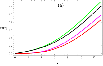
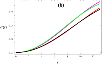
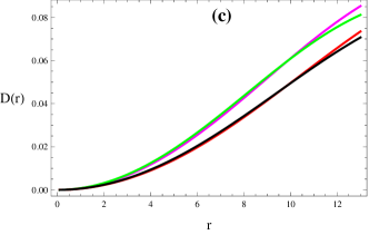
Figure 1: Plots of mass (in km) (a), compactness (b) and redshift (c) parameters corresponding to $\mathcal{S}=0.1,~{}\zeta=0.5$ (pink), $\zeta=0.9$ (green) and $\mathcal{S}=0.8,~{}\zeta=0.5$ (red), $\zeta=0.9$ (black) for solution-I

The $f(\mathcal{R},\mathcal{T},\mathcal{Q})$ theory comprises the complicated equations of motion due to the factor $\mathcal{Q}=\mathcal{R}_{\lambda\xi}\mathcal{T}^{\lambda\xi}$. Therefore for our convenience, we choose a linear model [16] to explore physical features of the developed solutions by taking arbitrary values of constant $\varrho$ as

$$f(\mathcal{R},\mathcal{T},\mathcal{R}_{\lambda\xi}\mathcal{T}^{\lambda\xi})=\mathcal{R}+\varrho\mathcal{R}_{\lambda\xi}\mathcal{T}^{\lambda\xi}.$$ (74)

The contraction of energy-momentum tensor with the Ricci tensor in the above model ensures that massive test particles in the gravitational field of self-gravitating model still entails the effects of non-minimal matter-geometry interaction. Here, the value of $\varrho$ can be negative or positive. The positive values of this arbitrary constant provide unacceptable behavior of the matter variables such as energy density and radial/tangential pressures corresponding to both the obtained solutions, as their values appear in negative range. Consequently, the solutions are no more viable as well as stable. Thus, we have the only choice for its negative values. First, we check the physical behavior of solution-I for $\varrho=-0.1$ and the constant $B$ defined in Eq.(53). The other two constants $A$ and $C$ are shown in Eqs.(40) and (42). We plot the graphs for mass, compactness and redshift of compact sphere (6) corresponding to the decoupling parameter $\zeta=0.5$ and $0.9$ in Figure 1. The mass shows increasing behavior with rise in $\zeta$ while charge decreases its value linearly. The particular values of $\zeta$ as well as charge confirm the compactness and redshift factors within their required limits, as shown in Figure 1 (b,c).

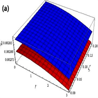
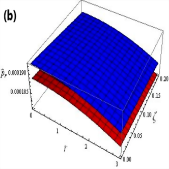
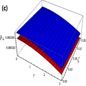
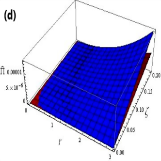
Figure 2: Plots of energy density (in km^-2) (a), radial pressure (in km^-2) (b), tangential pressure (in km^-2) (c) and anisotropy (in km^-2) (d) versus $r$ and $\zeta$ with $\mathcal{S}=0.1$ (Blue), $\mathcal{S}=0.8$ (Red), $\mathcal{M}=1M_{\bigodot}$ and $H=(0.2)^{-1}M_{\bigodot}$ for solution-I

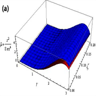
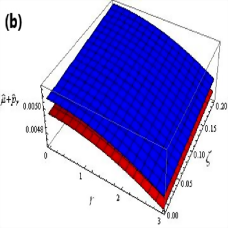
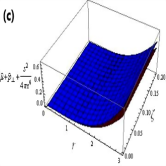
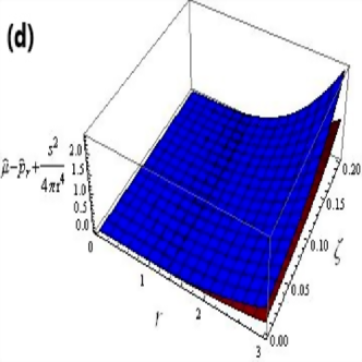
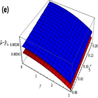
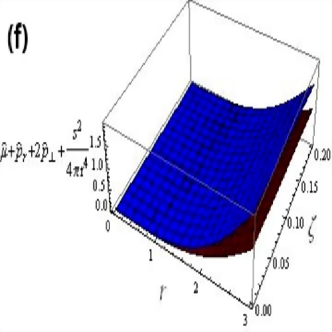
Figure 3: Plots of energy conditions (in km^-2) versus $r$ and $\zeta$ with $\mathcal{S}=0.1$ (Blue), $\mathcal{S}=0.8$ (Red), $\mathcal{M}=1M_{\bigodot}$ and $H=(0.2)^{-1}M_{\bigodot}$ for solution-I (a$-$f)

The values of material variables (pressure and energy density) for feasible structures should be maximum, positive and finite at the center while they show decreasing behavior towards the boundary of a star. Figure 2 (a) indicates the maximum value of energy density in the middle, whereas it shows decreasing behavior with the increment in $r$ as well as charge. Also, the behavior of effective energy density is monotonically rising as the decoupling parameter enhances which represents the more dense star for larger values of $\zeta$. Figure 2 displays that the plots of radial and tangential pressures show similar pattern for the parameter $\varrho$. Both graphs demonstrate the decrement with rise in all factors such as $r$, $\zeta$ and charge. The anisotropy $\hat{\Pi}$ disappears throughout the region for the decoupling parameter $\zeta=0$ and enhances as $\zeta$ increases which confirms that the additional source produces stronger anisotropy in the system. Evaluating the fundamental features of a self-gravitating star graphically by choosing different values of the coupling constant $\varrho$, we deduce that very small negative values of $\varrho$ provide the suitable behavior of physical variables. All energy conditions (72) corresponding to solution-I are satisfied, hence it is physically viable as illustrated in Figure 3. Figure 4 guarantees the stability of solution-I for different considered values of charge and the decoupling parameter. From Figure 4 (a), we find that the system becomes less stable with increment in charge near the boundary.

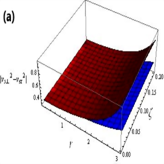
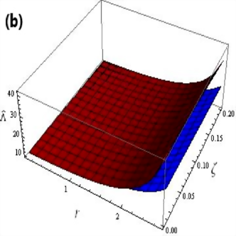
Figure 4: Plots of $|v_{s\bot}^{2}-v_{sr}^{2}|$ (a) and adiabatic index (b) versus $r$ and $\zeta$ with $\mathcal{S}=0.1$ (Blue), $\mathcal{S}=0.8$ (Red), $\mathcal{M}=1M_{\bigodot}$ and $H=(0.2)^{-1}M_{\bigodot}$ for solution-I

We now examine the feasibility of the obtained solution-II for $\varrho=-0.05$. Equations (40) and (65) depict the constants $A$ and $B$. We analyze the mass of geometry (6) for two values of the decoupling parameter $\zeta=0.1$ and $\zeta=0.25$, as given in Figure 5 (a). It is found that the mass increases with increasing $\zeta$, while the higher value of charge yields decreasing behavior. The same figure (b,c) also shows that the compactness $(\sigma(r))$ and redshift $(D(r))$ meet their required criteria for both values of charge. Figure 6 illustrates the physical behavior of different substantial variables as well as anisotropic factor. The effective energy density and both components of effective pressure show the same behavior as for the solution-I for particular values of charge and $\zeta$. In the absence of $\zeta$, anisotropy does not appear in the whole domain, while it increases with increase in $\zeta$, as shown in Figure 6 (d). Figure 7 guarantees the viability of our second solution as all energy conditions (72) are fulfilled. Figure 8 confirms the stability of solution-II for particular values of the parameter $\zeta$. It is noted from Figure 8 (a) that increment in charge leads to the less stable system for larger values of $\zeta$ near the boundary.

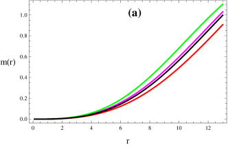
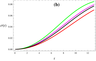
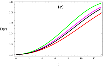
Figure 5: Plots of mass (in km) (a), compactness (b) and redshift (c) parameters corresponding to $\mathcal{S}=0.1,~{}\zeta=0.1$ (pink), $\zeta=0.25$ (green) and $\mathcal{S}=0.8,~{}\zeta=0.1$ (red), $\zeta=0.25$ (black) for solution-II

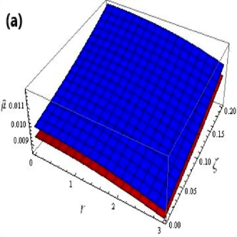
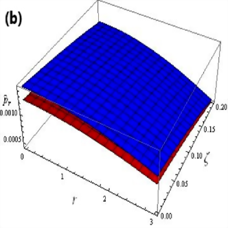
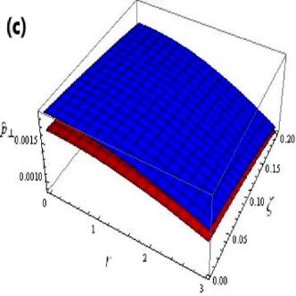
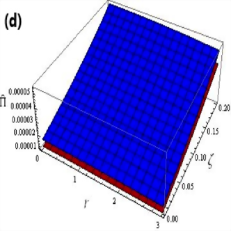
Figure 6: Plots of energy density (in km^-2) (a), radial pressure (in km^-2) (b), tangential pressure (in km^-2) (c) and anisotropy (in km^-2) (d) versus $r$ and $\zeta$ with $\mathcal{S}=0.1$ (Blue), $\mathcal{S}=0.8$ (Red), $\mathcal{M}=1M_{\bigodot}$ and $H=(0.2)^{-1}M_{\bigodot}$ for solution-II

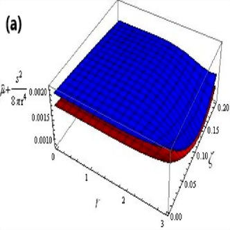
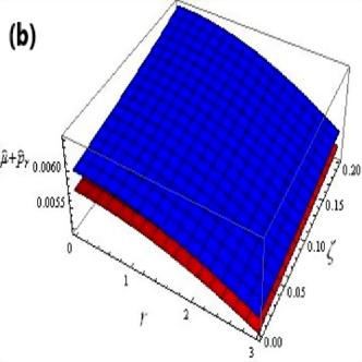
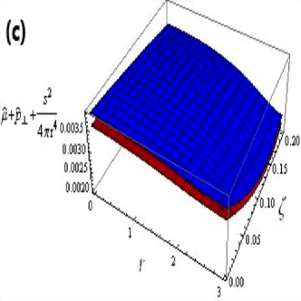
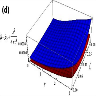
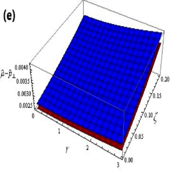
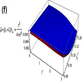
Figure 7: Plots of energy conditions (in km^-2) versus $r$ and $\zeta$ with $\mathcal{S}=0.1$ (Blue), $\mathcal{S}=0.8$ (Red), $\mathcal{M}=1M_{\bigodot}$ and $H=(0.2)^{-1}M_{\bigodot}$ for solution-II (a$-$f)

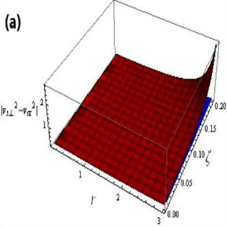
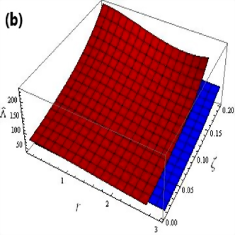
Figure 8: Plots of $|v_{s\bot}^{2}-v_{sr}^{2}|$ (a) and adiabatic index (b) versus $r$ and $\zeta$ with $\mathcal{S}=0.1$ (Blue), $\mathcal{S}=0.8$ (Red), $\mathcal{M}=1M_{\bigodot}$ and $H=(0.2)^{-1}M_{\bigodot}$ for solution-II

5 Conclusions

This paper aims to investigate various anisotropic solutions for a compact spherically symmetric geometry (6) with the help of EGD strategy. For this analysis, we take a linear model $\mathcal{R}+\varrho\mathcal{Q}$ in $f(\mathcal{R},\mathcal{T},\mathcal{Q})$ gravitational theory. The corresponding field equations have been developed and further split into two sets through the deformation functions. The first set represents an isotropic configuration, for which we have taken the isotropic Krori-Barua ansatz in this theory. The unknowns $A,~{}B$ and $C$ are computed using the matching conditions. To work out the second sector (22)-(24) involving five unknowns, we have used two constraints to make the system definite. The first one is the equation of state $\Upsilon^{0}_{0}=\tau\Upsilon^{1}_{1}+\upsilon\Upsilon^{2}_{2}$, where $\tau$ and $\upsilon$ are kept fixed, while the other is taken as pressure-like or density-like, leading to solutions-I and II, respectively.

To inspect the influence of the decoupling parameter as well as charge on the obtained solutions, we have discussed the graphical behavior of effective material variables $(\hat{\mu},\hat{p}_{r},\hat{p}_{\bot})$, pressure anisotropy $(\hat{\Pi})$ and energy conditions (72) for $\varrho=-0.1$ and $-0.05$. The redshift and compactness factors have also been found within their respective bounds. The compact geometry (6) becomes more massive with the increment of the decoupling parameter $\zeta$ for the both solutions, whereas the structure becomes less dense by increasing charge. We have utilized two different approaches to analyze the stability of these solutions. It is found that both solutions provide viable as well as stable geometry for particular values of $\zeta$ and charge. It is worthwhile to mention here that solution-I remains stable for the considered values of charge and $\zeta$, whereas solution-II becomes less stable with the increment in both these quantities near the boundary. However, the large values of charge may yield unstable system analogous to the first solution. We would like to mention here that this technique provides unstable solution corresponding to the density-like constraint in GR [59, 60] as well as $f(\mathcal{G})$ theory [61]. However, our resulting solutions show physically stable behavior even for larger values of $\zeta$. Moreover, the anisotropy does not vanish at the center in GR unlike $f(\mathcal{R},\mathcal{T},\mathcal{Q})$ framework. Thus we conclude that this modified gravity produces more suitable results. It can be said that extra force existing in $f(\mathcal{R},\mathcal{T},\mathcal{Q})$ theory could be the reason that offers differences of the consequences in this gravity from those in GR and other modified theories. Finally, for $\varrho=0$, all our results reduce to GR.

Appendix A

The modified matter components appearing in the field equations (10)-(12) are given as

$$\mathcal{T}_{0}^{0(\mathcal{D})} = \frac{1}{8\pi\big{(}f_{\mathcal{R}}+\mu f_{\mathcal{Q}}\big{)}}\left[\mu\left\{f_{\mathcal{Q}}\left(\frac{\chi^{\prime 2}}{2e^{\beta}}-\frac{\chi^{\prime}}{re^{\beta}}+\frac{\chi^{\prime}\beta^{\prime}}{4e^{\beta}}-\frac{\chi^{\prime\prime}}{2e^{\beta}}-\frac{1}{2}\mathcal{R}\right)+f^{\prime}_{\mathcal{Q}}\left(\frac{\chi^{\prime}}{2e^{\beta}}\right.\right.\right.$$

$$- \left.\left.\frac{\beta^{\prime}}{4e^{\beta}}+\frac{1}{re^{\beta}}\right)+\frac{f^{\prime\prime}_{\mathcal{Q}}}{2e^{\beta}}-2f_{\mathcal{T}}\right\}+\mu^{\prime}\left\{f_{\mathcal{Q}}\left(\frac{\chi^{\prime}}{2e^{\beta}}+\frac{1}{re^{\beta}}-\frac{\beta^{\prime}}{4e^{\beta}}\right)+\frac{f^{\prime}_{\mathcal{Q}}}{e^{\beta}}\right\}$$

$$+ \frac{f_{\mathcal{Q}}\mu^{\prime\prime}}{2e^{\beta}}+p\left\{f_{\mathcal{Q}}\left(\frac{3\beta^{\prime 2}}{4e^{\beta}}-\frac{2}{r^{2}e^{\beta}}-\frac{\beta^{\prime\prime}}{2e^{\beta}}\right)-f^{\prime}_{\mathcal{Q}}\left(\frac{5\beta^{\prime}}{4e^{\beta}}-\frac{1}{re^{\beta}}\right)+\frac{f^{\prime\prime}_{\mathcal{Q}}}{2e^{\beta}}\right\}$$

$$+ p^{\prime}\left\{f_{\mathcal{Q}}\left(\frac{1}{re^{\beta}}-\frac{5\beta^{\prime}}{4e^{\beta}}\right)+\frac{f^{\prime}_{\mathcal{Q}}}{e^{\beta}}\right\}+\frac{f_{\mathcal{Q}}p^{\prime\prime}}{2e^{\beta}}+\frac{\mathcal{R}f_{\mathcal{R}}}{2}+f^{\prime}_{\mathcal{R}}\left(\frac{\beta^{\prime}}{2e^{\beta}}-\frac{2}{re^{\beta}}\right)$$

$$- \left.\frac{f^{\prime\prime}_{\mathcal{R}}}{e^{\beta}}-\frac{f}{2}+\frac{q^{2}}{r^{4}}\left\{f_{\mathcal{T}}+\frac{f_{\mathcal{Q}}}{4e^{\beta}}\left(\chi^{\prime}\beta^{\prime}-2\chi^{\prime\prime}-\chi^{\prime 2}+\frac{4\beta^{\prime}}{r}\right)\right\}\right],$$

$$\mathcal{T}_{1}^{1(\mathcal{D})} = \frac{1}{8\pi\big{(}f_{\mathcal{R}}+\mu f_{\mathcal{Q}}\big{)}}\left[\mu\left(f_{\mathcal{T}}-\frac{f_{\mathcal{Q}}\chi^{\prime 2}}{4e^{\beta}}+\frac{f^{\prime}_{\mathcal{Q}}\chi^{\prime}}{4e^{\beta}}\right)+\frac{f_{\mathcal{Q}}\mu^{\prime}\chi^{\prime}}{4e^{\beta}}+p\left\{f_{\mathcal{T}}+f_{\mathcal{Q}}\left(\frac{\chi^{\prime\prime}}{e^{\beta}}\right.\right.\right.$$

$$- \left.\left.\frac{\beta^{\prime 2}}{e^{\beta}}+\frac{\chi^{\prime 2}}{2e^{\beta}}-\frac{3\chi^{\prime}\beta^{\prime}}{4e^{\beta}}-\frac{3\beta^{\prime}}{re^{\beta}}+\frac{2}{r^{2}e^{\beta}}+\frac{1}{2}\mathcal{R}\right)-f^{\prime}_{\mathcal{Q}}\left(\frac{\chi^{\prime}}{4e^{\beta}}+\frac{2}{re^{\beta}}\right)\right\}$$

$$- p^{\prime}f_{\mathcal{Q}}\left(\frac{\chi^{\prime}}{4e^{\beta}}+\frac{2}{re^{\beta}}\right)+\frac{f}{2}-\frac{\mathcal{R}f_{\mathcal{R}}}{2}-f^{\prime}_{\mathcal{R}}\left(\frac{\chi^{\prime}}{2e^{\beta}}+\frac{2}{re^{\beta}}\right)+\frac{q^{2}}{r^{4}}\left\{f_{\mathcal{T}}\right.$$

$$- \left.\left.\frac{f_{\mathcal{Q}}}{4e^{\beta}}\left(2\chi^{\prime\prime}+\chi^{\prime 2}-\chi^{\prime}\beta^{\prime}+\frac{4\chi^{\prime}}{r}\right)\right\}\right],$$

$$\mathcal{T}_{2}^{2(\mathcal{D})} = \frac{1}{8\pi\big{(}f_{\mathcal{R}}+\mu f_{\mathcal{Q}}\big{)}}\left[\mu\left(f_{\mathcal{T}}-\frac{f_{\mathcal{Q}}\chi^{\prime 2}}{4e^{\beta}}+\frac{f^{\prime}_{\mathcal{Q}}\chi^{\prime}}{4e^{\beta}}\right)+\frac{f_{\mathcal{Q}}\mu^{\prime}\chi^{\prime}}{4e^{\beta}}+p\left\{f_{\mathcal{T}}+f_{\mathcal{Q}}\left(\frac{\beta^{\prime\prime}}{2e^{\beta}}\right.\right.\right.$$

$$+ \left.\frac{\chi^{\prime}}{2re^{\beta}}-\frac{3\beta^{\prime 2}}{4e^{\beta}}-\frac{\beta^{\prime}}{2re^{\beta}}+\frac{1}{r^{2}e^{\beta}}-\frac{2}{r^{2}}+\frac{1}{2}\mathcal{R}\right)+f^{\prime}_{\mathcal{Q}}\left(\frac{3\beta^{\prime}}{2e^{\beta}}-\frac{\chi^{\prime}}{4e^{\beta}}-\frac{3}{re^{\beta}}\right)$$

$$- \left.\frac{f^{\prime\prime}_{\mathcal{Q}}}{e^{\beta}}\right\}+p^{\prime}\left\{f_{\mathcal{Q}}\left(\frac{3\beta^{\prime}}{2e^{\beta}}-\frac{\chi^{\prime}}{4e^{\beta}}-\frac{3}{re^{\beta}}\right)-\frac{2f^{\prime}_{\mathcal{Q}}}{e^{\beta}}\right\}-\frac{f_{\mathcal{Q}}p^{\prime\prime}}{e^{\beta}}-\frac{\mathcal{R}f_{\mathcal{R}}}{2}+\frac{f}{2}$$

$$+ \left.f^{\prime}_{\mathcal{R}}\left(\frac{\beta^{\prime}}{2e^{\beta}}-\frac{\chi^{\prime}}{2e^{\beta}}-\frac{1}{re^{\beta}}\right)-\frac{f^{\prime\prime}_{\mathcal{R}}}{e^{\beta}}\right].$$

The term $\Omega$ in Eq.(14) which occurs due to modified gravity is

$$\Omega =\frac{2}{\left(\mathcal{R}f_{\mathcal{Q}}+2(8\pi+f_{\mathcal{T}})\right)}\left[f^{\prime}_{\mathcal{Q}}e^{-\beta}\left(p-\frac{q^{2}}{8\pi r^{4}}\right)\left(\frac{1}{r^{2}}-\frac{e^{\beta}}{r^{2}}+\frac{\chi^{\prime}}{r}\right)+f_{\mathcal{Q}}e^{-\beta}\right.$$

$$\times\left(p-\frac{q^{2}}{8\pi r^{4}}\right)\left(\frac{\chi^{\prime\prime}}{r}-\frac{\chi^{\prime}}{r^{2}}-\frac{\beta^{\prime}}{r^{2}}-\frac{\chi^{\prime}\beta^{\prime}}{r}-\frac{2}{r^{3}}+\frac{2e^{\beta}}{r^{3}}\right)+\left(p^{\prime}-\frac{qq^{\prime}}{4\pi r^{4}}+\frac{q^{2}}{2\pi r^{5}}\right)$$

$$\times\left\{f_{\mathcal{Q}}e^{-\beta}\left(\frac{\chi^{\prime}\beta^{\prime}}{8}-\frac{\chi^{\prime\prime}}{8}-\frac{\chi^{\prime 2}}{8}+\frac{\beta^{\prime}}{2r}+\frac{\chi^{\prime}}{2r}+\frac{1}{r^{2}}-\frac{e^{\beta}}{r^{2}}\right)+\frac{3}{4}f_{\mathcal{T}}\right\}+\left(p-\frac{q^{2}}{8\pi r^{4}}\right)$$

$$\times f^{\prime}_{\mathcal{T}}-\left(\mu+\frac{q^{2}}{8\pi r^{4}}\right)f^{\prime}_{\mathcal{T}}-\left(\mu^{\prime}+\frac{qq^{\prime}}{4\pi r^{4}}-\frac{q^{2}}{2\pi r^{5}}\right)\left\{\frac{f_{\mathcal{Q}}e^{-\beta}}{8}\left(\chi^{\prime 2}-\chi^{\prime}\beta^{\prime}+2\chi^{\prime\prime}\right.\right.$$

$$+\left.\left.\frac{4\chi^{\prime}}{r}\right)+\frac{3f_{\mathcal{T}}}{2}\right\}-\left(\frac{e^{-\beta}}{r^{2}}-\frac{1}{r^{2}}+\frac{\chi^{\prime}e^{-\beta}}{r}\right)\left\{\left(\mu^{\prime}+\frac{qq^{\prime}}{4\pi r^{4}}-\frac{q^{2}}{2\pi r^{5}}\right)f_{\mathcal{Q}}+f^{\prime}_{\mathcal{Q}}\right.$$

$$\times\left.\left.\left(\mu+\frac{q^{2}}{8\pi r^{4}}\right)\right\}-\frac{1}{2}\left(f^{\prime}_{\mathcal{Q}}\mathcal{R}+f_{\mathcal{Q}}\mathcal{R}^{\prime}+2f^{\prime}_{\mathcal{T}}\right)\left(p-\frac{q^{2}}{8\pi r^{4}}\right)\right].$$

References

[1] S Nojiri and S D Odintsov Phys. Rev.
D68 123512 (2003)
[2] G Cognola, E Elizalde, S Nojiri, S D Odintsov and S Zerbini J. Cosmol. Astropart.
Phys.2005 010 (2005)
[3] Y S Song, W Hu and I Sawicki Phys.
Rev. D75 044004 (2007)
[4] M Akbar and R G Cai Phys.
Lett. B648 243 (2007)
[5] S Capozziello, M De Laurentis, S D Odintsov and A Stabile Phys. Rev. D83 064004 (2011)
[6] M Sharif and H R Kausar J. Cosmol. Astropart.
Phys.2011 022 (2011)
[7] M Sharif and H R Kausar J. Phys. Soc. Japan80 044004 (2011)
[8] S Arapoğlu, C Deliduman and K Y Ekşi J. Cosmol.
Astropart. Phys.2011 020 (2011)
[9] R Goswami, A M Nzioki, S D Maharaj and S G Ghosh Phys. Rev. D90 084011 (2014)
[10] M Sharif and Z Yousaf Astropart. Phys.56 19 (2014)
[11] M Sharif and Z Yousaf Astrophys. Space Sci.354 471 (2014)
[12] A V Astashenok, S Capozziello and S D Odintsov Phys. Rev. D89 103509 (2014)
[13] A V Astashenok, S Capozziello and S D Odintsov J. Cosmol. Astropart. Phys.2015 001 (2015)
[14] O Bertolami, C G Boehmer, T Harko and F S N Lobo Phys. Rev. D75 104016 (2007)
[15] T Harko, F S N Lobo, S Nojiri and S D Odintsov Phys. Rev. D84 024020 (2011)
[16] Z Haghani, T Harko, F S N Lobo, H R Sepangi and S Shahidi Phys. Rev. D88 044023 (2013)
[17] M Sharif and M Zubair J. Cosmol. Astropart. Phys.2013 042 (2013)
[18] M Sharif and M Zubair J. High Energy Phys.2013 79 (2013)
[19] S D Odintsov and D Sáez-Gómez Phys. Lett. B725 437 (2013)
[20] I Ayuso, J B Jiménez and A De la Cruz-Dombriz Phys. Rev. D91 104003 (2015)
[21] E H Baffou, M J S Houndjo and J Tosssa Astrophys. Space Sci.361 376 (2016)
[22] Z Yousaf, M Z Bhatti and T Naseer Eur. Phys. J. Plus135 353 (2020)
[23] Z Yousaf, M Z Bhatti and T Naseer Phys. Dark Universe28 100535 (2020)
[24] Z Yousaf, M Z Bhatti and T Naseer Int. J. Mod. Phys. D29 2050061 (2020)
[25] Z Yousaf, M Z Bhatti and T Naseer Ann. Phys.420 168267 (2020)
[26] Z Yousaf, M Z Bhatti, T Naseer and I Ahmad Phys. Dark Universe29 100581 (2020)
[27] Z Yousaf, M Y Khlopov, M Z Bhatti and T Naseer Mon. Not. R. Astron. Soc.495 4334 (2020)
[28] B Das, P C Ray, I Radinschi, F Rahaman and S Ray Int. J. Mod. Phys. D20 1675 (2011)
[29] J M Sunzu, S D Maharaj and S Ray Astrophys. Space Sci.352 719 (2014)
[30] M H Murad Astrophys. Space Sci.361 20 (2016)
[31] N Pant, R N Mehta and M J Pant Astrophys. Space Sci.332 473 (2011)
[32] Y K Gupta and S K Maurya Astrophys. Space Sci.332 155 (2011)
[33] M Sharif and M Z Bhatti Astrophys. Space Sci.347 337 (2013)
[34] M Sharif and Z Yousaf Phys. Rev. D88 024020 (2013)
[35] K N Singh and N Pant Astrophys. Space Sci.358 1 (2015)
[36] M Sharif and S Sadiq Eur. Phys. J. C76 1 (2016)
[37] M Sharif and A Siddiqa Eur. Phys. J. Plus132 1 (2017)
[38] M Sharif and A Waseem Gen. Relativ. Gravit.50 1 (2018)
[39] M Sharif and A Waseem Eur. Phys. J. Plus131 1 (2016)
[40] M Sharif and A Waseem Can. J. Phys.94 1024 (2016)
[41] S K Maurya, A Errehymy, D Deb, F Tello-Ortiz and M Daoud Phys. Rev. D100 044014 (2019)
[42] M F Shamir and I Fayyaz Theor. Math. Phys.202 112 (2020)
[43] J Ovalle Mod. Phys. Lett. A23 3247 (2008)
[44] J Ovalle and F Linares Phys. Rev. D88 104026 (2013)
[45] R Casadio, J Ovalle and R Da Rocha Class. Quantum Grav.32 215020 (2015)
[46] J Ovalle Phys. Rev. D95 104019 (2017)
[47] J Ovalle, R Casadio, R da Rocha, A Sotomayor and Z. Stuchlík Eur. Phys. J. C78 1 (2018)
[48] L Gabbanelli, Á Rincón and C Rubio Eur. Phys. J. C78 370 (2018)
[49] M Estrada and F Tello-Ortiz Eur. Phys. J. Plus133 1 (2018)
[50] M Sharif and S Sadiq Eur. Phys. J. C78 410 (2018)
[51] M Sharif and S Saba Eur. Phys. J. C78 921 (2018)
[52] M Sharif and S Saba Chin. J. Phys.59 481 (2019)
[53] M Sharif and A Waseem Ann. Phys.405 14 (2019)
[54] M Sharif and A Waseem Chin. J. Phys.60 426 (2019)
[55] K N Singh, S K Maurya, M K Jasim and F Rahaman Eur. Phys. J. C79 1 (2019)
[56] S Hensh and Z Stuchlík Eur. Phys. J. C79 1 (2019)
[57] J Ovalle Phys. Lett. B788 213 (2019)
[58] E Contreras and P Bargueño Class. Quantum Gravity36 215009 (2019)
[59] M Sharif and Q Ama-Tul-Mughani Ann. Phys.415 168122 (2020)
[60] M Sharif and Q Ama-Tul-Mughani Chin. J. Phys.65 207 (2020)
[61] M Sharif and S Saba Int. J. Mod. Phys. D29 2050041 (2020)
[62] M Sharif and T Naseer Chin. J. Phys.73 179 (2021)
[63] T Naseer and M Sharif Universe8 62 (2022)
[64] M Sharif and A Majid Phys. Dark Universe32 100803 (2021)
[65] M Sharif and A Majid Phys. Scr.96 035002 (2021)
[66] M Sharif and A Majid Phys. Scr.96 045003 (2021)
[67] K D Krori and J Barua J. Phys. A: Math. Gen.8 508 (1975)
[68] H A Buchdahl Phys. Rev.116 1027 (1959)
[69] B V Ivanov Phys. Rev. D65 104011 (2002)
[70] H Abreu, H Hernandez and L A Nunez Class. Quantum Gravit.24 4631 (2007)
[71] L Herrera Phys. Lett. A165 206 (1992)
[72] H Heintzmann and W Hillebrandt Astron. Astrophys.38 51 (1975)
[73] W Hillebrandt and K O Steinmetz Astron. Astrophys.53 283 (1976)