Dynamic MLP for Fine-Grained Image Classification
by Leveraging Geographical and Temporal Information

Abstract

Fine-grained image classification is a challenging computer vision task where various species share similar visual appearances, resulting in misclassification if merely based on visual clues. Therefore, it is helpful to leverage additional information, e.g., the locations and dates for data shooting, which can be easily accessible but rarely exploited. In this paper, we first demonstrate that existing multimodal methods fuse multiple features only on a single dimension, which essentially has insufficient help in feature discrimination. To fully explore the potential of multimodal information, we propose a dynamic MLP on top of the image representation, which interacts with multimodal features at a higher and broader dimension. The dynamic MLP is an efficient structure parameterized by the learned embeddings of variable locations and dates. It can be regarded as an adaptive nonlinear projection for generating more discriminative image representations in visual tasks. To our best knowledge, it is the first attempt to explore the idea of dynamic networks to exploit multimodal information in fine-grained image classification tasks. Extensive experiments demonstrate the effectiveness of our method. The t-SNE algorithm visually indicates that our technique improves the recognizability of image representations that are visually similar but with different categories. Furthermore, among published works across multiple fine-grained datasets, dynamic MLP consistently achieves SOTA results and takes third place in the iNaturalist challenge at FGVC8. Code is available at https://github.com/ylingfeng/DynamicMLP.git.

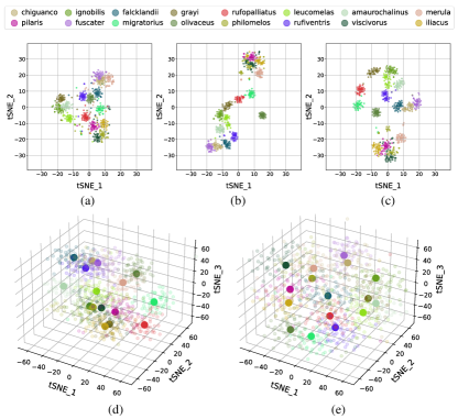
Figure 1: Visualization of t-SNE [44] representations under well trained models. Various similar species from the genus Turdus in the iNaturalist 2021 dataset are depicted in different colors. (a): The visualization of an image-only model. (b): Concatenating the image, location, and date features before the classification head is a typical strategy of utilizing additional information to help classification. The concatenated representation is more discriminative than the original. The concatenation strategy can be regarded as a baseline for all methods that involve additional information. (c): Intuitively, our proposed dynamic MLP expands the diversity among different fine-grained species compared to the image-only or concatenation framework. (d): The 3-d visualization of image representation from the concatenation strategy. (e): The 3-d visualization of our dynamic MLP.

1 Introduction

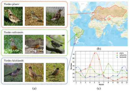
Figure 2: The pilaris, rufiventris, and falcklandii are species belonging to the genus Turdus. (a): They are visually similar and hard to recognize based on their appearance. (b): Their habitats vary widely. (c): Their activity frequency varies throughout the year, so the data amount at different times is different.

Fine-grained image classification [55, 1, 49, 53, 5, 54, 3] is a challenging computer vision task that distinguishes fine categories of objects or species. In contrast to traditional image classification [6, 18, 19, 50, 26], fine-grained image classification has difficulty identifying different species but with almost the same appearances. Those visually similar samples are practically impossible to differentiate if merely based on images. Apart from several popular fine-grained methods that focus on the discriminative regions of images [55, 49, 53, 54, 3], multi-branch learning [57, 5, 1, 13, 41], or particular data augmentations [25, 20], another available direction is to introduce additional information, e.g., geographical and temporal information, to help fine-grained image classification [37, 48, 8, 28].

Images usually contain additional information, e.g., geographic location and time, denoting where and when to shoot, which can help with fine-grained classification. For example, we choose three species from the genus Turdus, such as pilaris, rufiventris, and falcklandii, that are visually similar and thus difficult to distinguish (Fig. 2 (a)). However, their living locations (Fig. 2 (b)) and temporal distribution (Fig. 2 (c)) are quite different. It indicates that geographical and temporal information can be helpful to facilitate their accurate classification. Further, additional information such as locations or dates has already been provided in some well-known datasets like BirdSnap [4], PlantCLEF [15], YFCC100M [39], and iNaturalist [46, 45], and is widely available on the internet [14, 11, 21, 22].

Several works have proposed the use of additional information in fine-grained image classification. [37, 31, 38, 35, 29] directly concatenate the image feature with the multimodal feature before the final classification head. Furthermore, the addition [8] and multiplication [28, 38] operations are adopted to fuse the features or predictions from the last network layer. The core strategies are summarized in Fig. 3 (b)-(d), respectively. However, they only refer to a single dimension between image and multimodal features. As shown in Fig. 1 (a)-(b), the concatenation strategy only pulls the cluster apart vertically—in one dimension. More analysis can be found in Sec.3.3.

To fully exploit the potential effect of additional information, we propose to involve the higher-dimensional interaction between the multimodal representations. Evidently, since species with similar appearances have related image features extracted by the same network, a fixed projection fails to distinguish accurately if their categories are different. Especially when their locations are numerically close, existing multimodal methods technically lack the potential to make a distinction. Thus, a dynamic, instance-wise projection, which maps similar image features to different positions in the feature space, can manage to classify accurately. Different from existing works, we propose dynamic MLP to exploit the additional information in the form of adaptive perceptron weight to enhance the representation ability of image features (Fig. 3 (e)). Specifically, the weights of dynamic MLP are generated from the multimodal features extracted from the additional information. Then the image feature is updated by the dynamic MLP, where it is conditionally transformed by the adaptive weight. The projecting process in the dynamic MLP involves high-dimensional interaction between the image feature and multimodal feature and is verified to be more efficient in separating the decision boundaries of similar species. In Fig. 1, the clusters denoting similar categories are pulled apart in all directions evenly, which is more effective than the former work.

To verify the effectiveness of our proposed dynamic MLP, we conduct extensive experiments on four well-known fine-grained image classification datasets (iNaturalist 2017, 2018, 2021 [46, 45] and YFCC100M-GEO100 [39, 37]). Notably, our dynamic MLP consistently outperforms previous works by 0.2% $\sim$ 5.8% top-1 accuracy across a variety of popular benchmarks.

Overall, our contributions can be summarized as follows:

$\bullet$ We propose the dynamic MLP, an end-to-end trainable framework that jointly exploits images and additional information with high efficiency. To the best of our knowledge, we are the first to use dynamic MLP in multimodal fine-grained image classification tasks.

$\bullet$ Compared to existing published works, our method consistently achieves SOTA results on multiple datasets, specifically 76.81%, 83.67%, and 91.39% top-1 accuracy on iNaturalist 2017, 2018, and 2021, respectively.

$\bullet$ An ensemble of dynamic MLP reaches 94.75% top-1 accuracy on the iNaturalist 2021 dataset, which achieves 3rd place in the FGVC8 [10] at CVPR 2021.

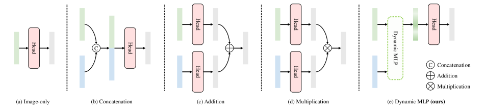
Figure 3: Comparisons of existing works with our dynamic MLP. The green and blue rectangles denote the image feature and multimodal feature, respectively. (a) Image-only: Get predictions based solely on images [18, 12, 26]. (b) Concatenation: Concatenate the image features with the multimodal features in a channel-by-channel fashion [37, 38, 35, 29]. (c) Addition: Add both predictions from the last layer of the image and extra information for a joint prediction [8]. (d) Multiplication: Multiply both predictions [28, 38]. (e) Dynamic MLP: Features are fused through the dynamic MLP.

2 Related Work

In this section, we review existing works on traditional fine-grained image classification that only deal with images. Then we summarize in fine-grained works that incorporate additional information. Finally, we introduce the development of the dynamic filter.

Fine-Grained Image Classification: To improve fine-grained image classification, several works have been proposed. [55, 49, 53, 54, 3] detect the discriminative regions of an image to explore subtle details. SnapMix [20] uses the class activation map (CAM) [58] to reduce the label noise in fine-grained data augmenting. Similarly, Attribute Mix [25] focuses on semantically meaningful attribute features from two images to identify the same super-categories. FixRes [42] investigates data augmentation and resolution to improve the classification performance. Other researches focus on extracting more useful features from multi-channel networks [57, 5] or contrastive learning [1, 13]. TransFG [17] and TPSKG [27] have recently used the Transformer architecture to improve classification performance. The fine-grained methods generally suffer from a complex pipeline and enormous manual design. Moreover, most existing methods depend on large training resolution to perform effectively, which is incompatible with large datasets like iNaturalist. Our dynamic MLP can operate efficiently on the most basic baseline without particular training settings.

Methods using Additional Information: Besides visual information, researchers have included additional information to improve classification performance. Many existing works [37, 31, 38, 35, 29] combine the image feature with the additional multimodal feature directly through channel-wise concatenation. [37] is the first to introduce multimodal features, e.g., images, ages, and dates, extracted from MLP backbone network by concatenating them together to make a joint prediction. Later, [31] introduces metadata to the geospatial land classification task, and [35] integrates dense overhead imagery with location and date into a general framework by concatenating the outputs of the context network. The concatenation methods share the projection weight for all samples, while our proposed dynamic MLP can perform an intrinsic, instance-wise transform to the image representation guided by additional information. Another fusion strategy aims to combine the output predictions of images and metadata through multiplication or addition operations. [28] extracts location features by MLP to produce a prior distribution for fine-tuning the original predictions. In GeoNet [8], the geolocation priors, post-processing models, and feature modulation models are utilized to leverage the additional information. [38] ensembles the result by multiplying the relative categorization probabilities. These methods often handle images and additional information separately, which could easily fall into a local optimum. In contrast, our framework is end-to-end trainable. Therefore, it could learn the most discriminative representations for classification through joint backpropagation. Using a knowledge graph is another way to handle additional information. [48] recommends a list including the most likely categories related to metadata based on a geo-aware database. [32] constructs a geospatial concept graph that contains the prior information for realizing the geo-aware classification. Since these methods are attached to a complex geographical or temporal knowledge graph, they often consume enormous memory costs and require specific manual design.

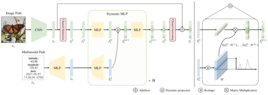
Figure 4: An overview of our proposed framework. It contains two paths for image and relational information, respectively. The dynamic MLP (in this figure a variant B is depicted) fuses two paths and produces the enhanced image representation. The core of dynamic MLP is a dynamic projection, indicated as “D”, which transforms the image representation by parameters adaptively generated from the multimodal feature. The dynamic MLP is employed recursively, where “$N$” denotes the stage number.

Dynamic Filters: Dynamic filters are adaptively modulated based on the input features, showing impressive performance across various vision tasks. CondConv [51], DyNet [56], and Dynamic Conv [7] learn dynamic parameters for multiple selective kernels. [23, 16] dynamically generates the filters, in which the weights are conditioned on the input images. Recently, Sparse R-CNN [36], SOLOv2 [47], and CondInst [40] extend the idea to object detection and instance segmentation, and [52, 30, 33] explore the usage in vision-language multimodal tasks. In general, existing works derive dynamic filters from a single source, such as images. Besides, they all deal with multimodal features between spatial feature maps [34] or queries of textual embeddings [52, 30, 33], which cannot be directly applied to multimodal fine-grained classification. Different from previous methods, our method introduces external information, i.e., locations and dates. To the best of our knowledge, we are the first to use dynamic projection in fine-grained image classification to fuse the additional information.

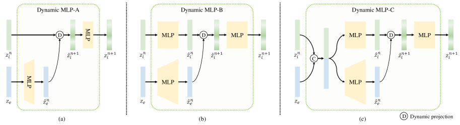
Figure 5: Comparisons between the three versions of dynamic MLP. (a) depicts the basic version and (b) expands the MLP depth. The image feature and multimodal feature in (a) and (b) are separately embedded, while they are concatenated together before projecting in (c).

3 Method

In this section, we introduce a bilateral-path framework for multimodal fine-grained image classification that fuses additional information effectively. The framework contains an image path and a multimodal path, taking as input the image and additional information, respectively. First, the image feature is extracted by a CNN, whilst the multimodal feature is derived through the MLP backbone network. The adaptive projection with weighted multimodal features is then used to update it within a group of dynamic MLPs. The refined image representation produces the final prediction. Next, we elaborate on three dynamic MLP variants. Specifically, they are structures with basic implementation, with deeper embedding layers, and with concatenation inputs. Finally, we analyze the degree of interaction with multimodal information based on various methods.

3.1 Framework

We design two paths in our architecture (Fig. 4), the image path and the multimodal path, for processing the image and additional information, respectively, based on existing works with additional information. Different from previous works, we propose a novel multimodal fusion method, termed “dynamic MLP”, to refine and enhance the image representation based on the additional information. We mark the original image feature after global average pooling as $\textbf{z}_{i}$ and the multimodal feature as $\textbf{z}_{e}$, providing the input image as $\textbf{x}_{i}$, and the additional information as $\textbf{x}_{e}$, respectively. Our structure is designed as a recursive architecture since more dynamic projections can lead to better performance experimentally. $\textbf{z}_{i}^{n}$ is defined in the following sections as the image representation updated $n$ times by the dynamic MLP, where $n\in\{1,2,...,N\}$.

Specifically, given the input image $\textbf{x}_{i}$, we can obtain its original embedding $\textbf{z}_{i}$ through the CNN backbone network, following the image path. Simultaneously, the multimodal path accepts additional information as input, such as latitude, longitude, and date, and obtains multimodal features $\textbf{z}_{e}$ via a residual MLP backbone network. In detail, the additional information is first normalized to $[-1,1]$ and is then concatenated channel-wise:

$$\hat{\textbf{x}}_{e}=\mathrm{Concat}(\{lat,lon,date\}),$$ (1)

where $lat$, $lon$, and $date$ denote the latitude, longitude, and date related to an image, respectively. $\mathrm{Concat}(\cdot)$ denotes the channel-wise concatenation and $\hat{\textbf{x}}_{e}\in\mathbb{R}^{3}$ denotes the intermediate encoding result of the additional information. Then the additional information $\hat{\textbf{x}}_{e}$ is mapped to $\textbf{x}_{e}\in\mathbb{R}^{6}$:

$$\textbf{x}_{e}=[\mathrm{Sin}(\pi\hat{\textbf{x}}_{e}),\mathrm{Cos}(\pi\hat{\textbf{x}}_{e})],$$ (2)

where $\mathrm{Sin(\cdot)}$ and $\mathrm{Cos(\cdot)}$ denote the sine and cosine functions, respectively. Finally, the multimodal feature $\textbf{z}_{e}$ is extracted by a residual MLP backbone network, following the descriptions in PriorsNet [28].

After the image and multimodal features are obtained, they are fused via the dynamic MLP. To save memory costs and runtime, the image feature is reduced to ${z}_{i}^{0}$ with lower dimensions by a channel-reduction layer. The dynamic MLP takes $\textbf{z}_{i}^{0}$ and $\textbf{z}_{e}$ as the initial inputs, where the image feature is dynamically projected by the corresponding multimodal feature. We obtain the enhanced image representation $\textbf{z}_{i}^{N}$ after $N$ recursive dynamic MLP blocks. The details of dynamic MLP are elaborated in Sec.3.2. Next, $\textbf{z}_{i}^{N}$ is expanded to align the shape with the original input $\textbf{z}_{i}$ by a channel-increasing layer. Then we employ a skip connection between the adjusted and original features to produce the final predictions.

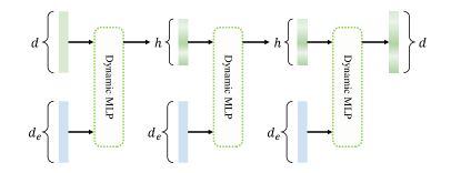
Figure 6: The channel width in dynamic MLP, which resembles a bottleneck architecture ($N=3$).

The whole framework not only learns to extract high-quality visual contextual clues but also tries to focus on optimal attention through image representations based on the guidance of multimodal features. Different from the traditional convolution layer or linear layer, the parameters of which are fixed for all instances, the projector’s weights in our framework are dynamically generated and conditioned based on the instance-wise additional information. It eases the recognition difficulty if two different species are similar in appearance. Essentially, our dynamic MLP fuses the multimodal features into a higher and broader dimensions than the single dimension produced by the former methods, which is further discussed in Sec.3.3. Through end-to-end optimization, our network can learn more generalized and discriminative features, which significantly outperforms the baseline image-only network as well as surpasses existing published works that utilize additional information in ordinary ways.

Backbone	Method	Reference	YFCC-GEO		iNat18		iNat21 Mini		iNat21 Full
ResNet-50	Baseline	–	47.650	77.950	64.345	85.348	67.924	86.563	79.830	93.363
	ConcatNet [37]	ICCV 2015	47.600	78.600	77.135	92.754	78.326	92.456	87.183	96.639
	PriorsNet [28]	ICCV 2019	41.850	72.250	70.097	86.625	78.019	92.362	86.784	96.523
	GeoNet [8]	ICCV 2019	48.800	80.000	75.035	91.169	77.738	91.875	86.727	96.229
	EnsembleNet [38]	MEE 2020	50.800	81.950	73.692	89.769	72.148	87.926	87.595	96.519
	Dynamic MLP (ours)	–	53.200	83.850	78.220	93.433	78.751	92.896	87.283	96.749
ResNet-101	Baseline	–	52.650	83.050	66.953	87.440	70.710	88.477	82.080	94.639
	ConcatNet [37]	ICCV 2015	52.800	84.050	78.576	93.585	80.564	93.582	88.494	97.135
	PriorsNet [28]	ICCV 2019	47.650	77.150	72.521	87.632	80.111	93.433	88.439	97.135
	GeoNet [8]	ICCV 2019	53.800	84.350	76.529	92.418	79.165	92.700	87.987	96.747
	EnsembleNet [38]	MEE 2020	52.550	84.400	76.934	91.501	75.295	89.775	88.800	96.941
	Dynamic MLP (ours)	–	54.500	84.450	79.248	93.847	80.574	93.860	88.482	97.245
SK-Res2Net-101	Baseline	–	54.400	83.500	74.150	91.710	76.102	91.456	86.178	96.400
	ConcatNet [37]	ICCV 2015	55.550	85.600	82.081	94.874	83.706	94.932	91.200	97.992
	PriorsNet [28]	ICCV 2019	50.600	78.800	77.720	90.129	83.600	94.925	90.773	98.010
	GeoNet [8]	ICCV 2019	56.050	84.950	78.912	93.740	81.360	93.712	90.070	97.602
	EnsembleNet [38]	MEE 2020	53.800	82.750	80.468	93.421	80.277	92.743	91.137	97.831
	Dynamic MLP (ours)	–	56.800	85.950	83.673	95.636	84.694	95.337	91.397	98.213

Table 1: Comparisons to previous SOTA multimodal works on the YFCC100M-GEO100 [37] and the iNaturalist 2018, 2021 [46, 45] datasets. For each experiment, we present the top-1 (left) and top-5 (right) accuracy.

Type	Method	Flops	#Params	Res	Acc (%)
Image-only	Baseline	8.9 G	56.8 M	224	71.0
	FixSENet [43]	20.8 G	123.5 M	224*	75.4
	TransFG [17]	49.2 G	90.04 M	304	71.7
Multimodal	ConcatNet [37]	8.9 G	58.7 M	224	76.3
	PriorsNet [28]	8.9 G	58.6 M	224	71.1
	GeoNet [8]	8.9 G	58.6 M	224	74.0
	EnsembleNet [38]	8.9 G	58.6 M	224	73.8
	Dynamic MLP (ours)	8.9 G	64.1 M	224	76.8

Table 2: We report the best-published result of a single model from state-of-the-art fine-grained image-only methods and multimodal methods on the iNaturalist 2017 dataset. “Res” denotes the input image resolution. *The test resolution in FixSENet [43] is larger than the training phase which brings extra gain in performance.

3.2 Dynamic MLP Structures

In this section, we first describe the elementary implementation of our proposed dynamic MLP (Fig. 5 (a)). Then two of its improved variants (Fig. 5 (b)-(c)) are discussed.

Dynamic MLP-A: Inspired by dynamic filters [23, 51, 56, 7, 36], we propose an iterable structure, namely dynamic MLP, which adaptively promotes the representation ability of the image feature guided by the multimodal feature. In Fig. 5 (a), we show a single unit of dynamic MLP-A, the most concise implementation of dynamic MLP. Each input image feature for the current dynamic MLP block is the output of the former block. For the multimodal input for each block, we uniformly use the original feature. Notably, all the recursive blocks of dynamic MLP are identical except for their channel dimensions. We create a bottleneck architecture (Fig. 6) by specifying a smaller hidden channel ($h$) for the intermediate dynamic MLP blocks than the original input dimension ($d$). Experimentally, the detailed channel settings are discussed in Table 3.

Specifically, it takes as input the image and multimodal feature and outputs the projected image feature for one iteration. First, the weight of the dynamic projector is generated based on the multimodal feature:

$$\mathbf{W}=\mathrm{Reshape}(f(\textbf{z}_{e})),$$ (3)

where $\mathrm{Reshape}(\cdot)$ reformulates a 1-d feature into a 2-d matrix, and $f(\cdot)$ denotes the fully connected layer. The following MLP structure can be illustrated as:

$$\textbf{z}_{i}^{n+1}=\mathrm{ReLU}\big{(}\mathrm{LN}(f(\textbf{z}_{i}^{n};\mathbf{W}))\big{)},$$ (4)

where $\mathrm{ReLU}(\cdot)$ and $\mathrm{LN}(\cdot)$ denote ReLU activation function and layer normalization [2], respectively. Notably, the above process is iterated until $N$ recursions are completed.

Dynamic MLP-B: In Fig. 5 (b), we exploit a deeper-in-depth version of dynamic MLP-A by expanding MLP layers. The extended MLP blocks are simple sequences of regular fully connected layers, layer normalization [2], and ReLU activation function.

Dynamic MLP-C: The inputs for the above structures are non-interactive until the dynamic projection. However, in dynamic MLP-C (Fig. 5 (c)), the inputs are concatenated together channel-wise before any of the embedding layers. Since the image feature and multimodal feature have mutual information supplement potential, we speculate that they can jointly generate better conditional weight to guide the transformation of image representation. Additionally, we perform an ablating study on the situations where only one input is replaced by the concatenated feature while the other remains unchanged, which is discussed in Table 5.

3.3 Interactive Dimensions

In this section, we compare the differences in interactive dimensions on multimodal features between previous works and our dynamic MLP. We aim to demonstrate that previous works have limitations in enlarging the distance of image representations in the feature space. As for the concatenation strategy, given the image feature $\textbf{z}_{i}\in\mathbb{R}^{d_{i}}$ and multimodal feature $\textbf{z}_{e}\in\mathbb{R}^{d_{e}}$, where $d_{i}$ and $d_{e}$ are the feature channels, we can extend ${z}_{i}$ and ${z}_{e}$ to the “$d_{i}+d_{e}$” dimension by padding zeros: $\textbf{z}^{\prime}_{i}=\{\textbf{z}_{i}^{1},...,\textbf{z}_{i}^{d_{i}},0,...,0\}$, where $d_{e}$ zeros are padded after ${z}_{i}$. In the same way we can get $\textbf{z}^{\prime}_{e}=\{0,...,0,\textbf{z}_{e}^{1},...,\textbf{z}_{e}^{d_{e}}\}$ with $d_{i}$ zeros. Then the final predictions can be derived as:

$$y=h(\mathrm{Concat}(\{\textbf{z}_{i},\textbf{z}_{e}\}))=h(\textbf{z}^{\prime}_{i}+\textbf{z}^{\prime}_{e}),$$ (5)

where y denotes the prediction and $h(\cdot)$ the classifier head, respectively. The fusion procedure of the addition strategy is exactly an element-wise addition between dual outputs:

$$y=h(\textbf{z}_{i})+h(\textbf{z}_{e}).$$ (6)

Similarly, the multiplication strategy can be depicted as:

$$y=h(\textbf{z}_{i})\cdot h(\textbf{z}_{e})=exp(log(h(\textbf{z}_{i}))+log(h(\textbf{z}_{e}))).$$ (7)

The common characteristic of the previous fusion strategy is essentially to add the representation or predictions based on images, locations, and dates, which involves only one dimension within multimodal features. Different from the former methods, the weights of dynamic MLP are adaptively generated from the location and date, and the dynamically refined image representation is obtained after an instance-wise projection between the original image representation and the weighted features of locations and dates:

$$y=h(f(\textbf{z}_{i},\textbf{z}_{e}))=h(\Sigma{(\textbf{z}_{i}^{:}\cdot\textbf{z}_{e}^{:,1})},...,\Sigma{(\textbf{z}_{i}^{:}\cdot\textbf{z}_{e}^{:,d_{i}})}).$$ (8)

The analysis indicates that our fusion strategy introduces a higher-dimensional interaction. As a result, it separates the cluster of image representations to a larger extent in all directions (Fig. 1).

4 Experiment

We conduct experiments on four fine-grained benchmark datasets that have collected additional information (iNaturalist 2017, 2018, 2021 [46, 45] and YFCC100M-GEO100 [37]). Notably, for a few images with unavailable metadata (corrupted or missing) in the dataset, we compensate with initialized zero input. To evaluate the effectiveness of our dynamic MLP, we compare it with state-of-the-art fine-grained methods with and without utilizing additional information. Furthermore, the ablation study and related analysis are conducted to better illustrate the network components of dynamic MLP.

$d$	$h$	iNat21 Mini		iNat21 Full
0	–	76.102	91.456	86.178	96.400
256	32	84.126	95.302	91.197	98.072
	64	84.341	95.275	91.329	98.152
	128	84.252	95.345	91.216	98.068
	256	84.213	95.275	91.314	98.120
64	64	83.971	95.126	91.190	98.034
128		84.006	95.209	91.023	98.045
256		84.341	95.275	91.329	98.152
512		84.164	95.301	91.284	98.106

Table 3: Top-1 (left) and top-5 (right) accuracy under various $d$ and $h$ with $N=2$, while $d=0$ denotes the baseline (image-only).

Stage Number ($N$)	iNat21 Mini		iNat21 Full
1	84.186	95.322	91.181	98.090
2	84.341	95.275	91.329	98.152
3	84.052	95.200	91.293	98.131
4	84.100	95.300	91.249	98.120

Table 4: Comparisons among different stage numbers.

Implementation Details: During training, unless otherwise stated, the dynamic MLP and other existing works are both trained with the Stochastic Gradient Descent (SGD) algorithm based on the ResNet-50 [18], ResNet-101 [18], and SK-Res2Net-101 [26, 12] backbones for fair comparisons. During inference, we apply a center crop to the image as the data augmentation. More experimental details can be found in the Supplementary Materials.

4.1 Comparisons with State-of-the-arts

Table 1 shows the top-1 and top-5 classification accuracy of our dynamic MLP (specifically refer to the dynamic MLP-C) and other approaches on various fine-grained datasets. Specifically, we reproduce PriorsNet [28] following their official descriptions under unified backbones for a fair comparison. The hyperparameter in the post-processing method of GeoNet [8] follows the settings in FGTL [9]. More detailed settings of our re-implementation can be found in the Supplementary Materials. Our dynamic MLP consistently achieves SOTA results on multiple datasets. On the iNaturalist 2021 dataset, we achieve a highly competitive 91.40% top-1 accuracy using SK-Res2Net-101. Additionally, it is noticed that the gap between our method and others is even more obvious for a bigger backbone model. For example, when changing the backbone from ResNet-50 to SK-Res2Net-101, the accuracy of ConcatNet [37] increases by 5.38% while ours is 5.94% on the iNaturalist 2021 mini dataset. Since dynamic MLP transforms image features under the guidance of multimodal features, we suspect that a bigger backbone can facilitate the dynamic MLP to explore stronger feature correlations and achieve more improvement compared to other methods. Next, we compare our methods on the iNaturalist 2017 dataset with the best-published results from state-of-the-art fine-grained image-only methods [43, 17]. Table 2 shows that dynamic MLP outperforms existing works which even necessitate higher memory costs, more complex pipelines, and higher training or testing resolution.

In the iNaturalist 2021 challenge at FGVC8 [10], we experiment with our dynamic MLP based on CNN and Transformer backbones with multiple image resolutions. During inference, we employ multi-scale testing and standard Ten-crop [24] as post-processing strategies. The ensemble result achieves 94.75% top-1 accuracy on the iNaturalist 2021 benchmark [10]. See more detailed results in the Supplementary Materials.

Method	Ver	IP	MP	iNat21 Mini		iNat21 Full
Baseline	–	–	–	76.102	91.456	86.178	96.400
Dynamic MLP	A			84.341	95.275	91.329	98.152
	B			84.406	95.403	91.244	98.118
	C		✓	84.443	95.357	91.212	98.160
	C	✓		84.573	95.337	91.235	98.132
	C	✓	✓	84.694	95.337	91.397	98.213

Table 5: Comparisons between different dynamic MLP structures. “Ver” denotes the version. “IP” and “MP” indicate the input feature type for the image path and multimodal path, respectively. “✓” means the input is replaced with the concatenated feature.

Method	Flops	#Params	Top-1	Top-5
(a) Baseline	8.9 G	66.8 M	76.102	91.456
(b) Concatenation	8.9 G	70.0 M	83.706	94.932
(b) Concatenation*	8.9 G	74.2 M	83.915	94.893
(c) Addition	8.9 G	69.9 M	84.010	94.935
(c) Addition*	8.9 G	74.2 M	84.068	94.982
(d) Multiplication	8.9 G	69.9 M	80.277	92.743
(d) Multiplication*	8.9 G	74.2 M	81.649	93.421
(e) Dynamic MLP (ours)	8.9 G	74.2 M	84.694	95.337

Table 6: Comparisons of our dynamic MLP and existing multimodal fusion methods on the iNaturalist 2021 mini dataset. (a): Baseline. (b): Concatenation. (c): Addition. (d): Multiplication. (e): Dynamic MLP. *Compensated models with the same flops and parameter numbers as our dynamic MLP.

4.2 Ablation Study

Channel Dimension (i.e., $d$, $h$): We first examine the impact of input and hidden channel dimensions (Fig. 6) on dynamic MLP-A on classification performance. Specifically, we explore their effect by fixing one and adjusting the other in Table 3. The experiments are conducted based on the SK-Res2Net-101 backbone on the iNaturalist 2021 dataset. It is observed that $d=256$, $h=64$ steadily achieve higher accuracy compared to other dimension combinations. We assume that a higher dimension may lead to overfitting of the network, while $d=256$, $h=64$ are sufficient to derive considerable discriminative representations.

Stage Number (i.e., $N$): We then explore the best stage number for dynamic MLP-A by setting it under $d=256$ and $h=64$. Table 4 shows that $N=2$ achieves the best performance trade-off, avoiding the overfitting risks with more stages applied. Therefore, we default to using $N=2$ in the following experiments.

Comparison of Structures: In this section, we compare the dynamic-MLP-A with its two variants (Fig. 5) based on the optimal settings ($d=256$, $h=64$, $N=2$). Table 5 indicates that the dynamic MLP-C achieves superior performance on fine-grained image classification, which is in line with our expectations that a deeper MLP projection and a concatenated operation before feature fusion can further benefit our architecture.

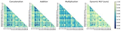
Figure 7: Visualization of the L2 distance between each two feature representations of sampled categories. A lighter color denotes a farther distance and better distinction.

Comparison of Fusion Strategies: To verify the effectiveness of our method, we compare our dynamic MLP (e) with the baseline (a) and various existing fusion strategies, i.e., concatenation (b), addition (c), and multiplication (d) (Fig. 3). Specifically, we use dynamic MLP-C and fix its channel dimension and stage number to the optimal settings ($d=256$, $h=64$, $N=2$) for all experiments on the iNaturalist 2021 mini dataset. Notably, our model has higher flops and parameter numbers. For a fair comparison, we compensate the networks of previous methods with additional MLP layers. The adjusted models have the same flops and parameters as ours. As shown in Table 6, our dynamic MLP outperforms previous work under the unified model capacity setting.

4.3 Analysis

Although the dynamic MLP is demonstrated to improve the performance across multiple fine-grained datasets, we would like to understand how its mechanism operates. More analyses can be found in the Supplementary Materials.

Visualization of T-SNE Representations: We evaluate 16 species from the genus Turdus in the iNaturalist 2021 dataset and visualize their image representations as points based on well-trained models of different methods, respectively. Fig. 1 shows that our dynamic MLP produces more discriminative image representations than previous works. As illustrated in Sec.3.3, former works fuse image and location features into one dimension, which is insufficient for separating the mutual representations. It is also shown in Fig. 1 (b) that the concatenation strategy stretches the cluster distribution only in one direction. Since dynamic MLP transforms the image representation by weighted features generated from the additional information, it involves mutual interaction on a broader dimension. Therefore, it improves the representation ability of the feature to benefit fine-grained image classification.

Visualization of L2 Distance Between Image Representations: Each row of the classifier weight is a representative feature corresponding to a specific category. To measure the instance representations quantitatively, we calculate the L2 distance between every two of the class-wise representative features and produce the heatmap visualization. Fig. 7 shows that the dynamic MLP can have more discriminant feature representations.

Training/Inference Efficiency: Table 7 shows the training and inference efficiency of existing multimodal methods and our dynamic MLP on the iNaturalist 2021 mini dataset. Specifically, GeoNet [8] is extremely time-consuming as its framework requires fine-tuning on a pretrained image-only model. Notably, our proposed dynamic MLP achieves top performance (84.694%) while still maintaining competitive training and inference efficiency.

Method	Acc (%)	H $\downarrow$	FPS $\uparrow$
Baseline	76.102	30.0	19.3
ConcatNet [37]	83.706	32.5	18.4
PriorsNet [28]	83.600	31.5	19.3
GeoNet [8]	81.360	55.0	19.0
EnsembleNet [38]	80.277	31.5	18.4
Dynamic MLP (ours)	84.694	32.0	18.4

Table 7: Comparisons of training and inference efficiency. “H” denotes the total training hours for 90 epochs on iNaturalist 2021 mini dataset evaluated on 8 TITAN Xp GPUs. “FPS” denotes the inference FPS measured on the same machine.

5 Conclusion

In this paper, we propose an end-to-end trainable framework, i.e., the dynamic MLP, to improve the effectiveness of geographical and temporal information on fine-grained image classification. Our method adaptively projects image representations by weights conditioned on additional information, which involves high-dimensional feature interaction. To our best knowledge, we are the first to introduce dynamic MLP in multimodal fine-grained image classification. Notably, our method achieves SOTA results on multiple fine-grained datasets. Further, the t-SNE visualization verifies that its image representations are more discriminative than previous works. We hope dynamic MLP can serve as a lightweight yet effective baseline for multimodal fine-grained image classification.

Acknowledgement. This work was supported by Postdoctoral Innovative Talent Support Program of China under Grant BX20200168, 2020M681608, and National Science Fund of China under Grant No. U1713208.

References

- [1] Zeynep Akata, Scott Reed, Daniel Walter, Honglak Lee, and Bernt Schiele. Evaluation of output embeddings for fine-grained image classification. In CVPR, 2015.
- [2] Jimmy Lei Ba, Jamie Ryan Kiros, and Geoffrey E Hinton. Layer normalization. arXiv preprint arXiv:1607.06450, 2016.
- [3] Ardhendu Behera, Zachary Wharton, Pradeep Hewage, and Asish Bera. Context-aware attentional pooling (cap) for fine-grained visual classification. arXiv preprint arXiv:2101.06635, 2021.
- [4] Thomas Berg, Jiongxin Liu, Seung Woo Lee, Michelle L Alexander, David W Jacobs, and Peter N Belhumeur. Birdsnap: Large-scale fine-grained visual categorization of birds. In CVPR, 2014.
- [5] Dongliang Chang, Yifeng Ding, Jiyang Xie, Ayan Kumar Bhunia, Xiaoxu Li, Zhanyu Ma, Ming Wu, Jun Guo, and Yi-Zhe Song. The devil is in the channels: Mutual-channel loss for fine-grained image classification. IEEE TIP, 2020.
- [6] Tianqi Chen, Mu Li, Yutian Li, Min Lin, Naiyan Wang, Minjie Wang, Tianjun Xiao, Bing Xu, Chiyuan Zhang, and Zheng Zhang. Mxnet: A flexible and efficient machine learning library for heterogeneous distributed systems. arXiv preprint arXiv:1512.01274, 2015.
- [7] Yinpeng Chen, Xiyang Dai, Mengchen Liu, Dongdong Chen, Lu Yuan, and Zicheng Liu. Dynamic convolution: Attention over convolution kernels. In CVPR, 2020.
- [8] Grace Chu, Brian Potetz, Weijun Wang, Andrew Howard, Yang Song, Fernando Brucher, Thomas Leung, and Hartwig Adam. Geo-aware networks for fine-grained recognition. In ICCV, 2019.
- [9] Yin Cui, Yang Song, Chen Sun, Andrew Howard, and Serge Belongie. Large scale fine-grained categorization and domain-specific transfer learning. In CVPR, 2018.
- [10] FGVC8. https://www.kaggle.com/c/inaturalist-2021, 2021.
- [11] Flickr. http://www.flickr.com, 2004.
- [12] Shanghua Gao, Ming-Ming Cheng, Kai Zhao, Xin-Yu Zhang, Ming-Hsuan Yang, and Philip HS Torr. Res2net: A new multi-scale backbone architecture. IEEE TPAMI, 2019.
- [13] Yu Gao, Xintong Han, Xun Wang, Weilin Huang, and Matthew Scott. Channel interaction networks for fine-grained image categorization. In AAAI, 2020.
- [14] GBIF. http://www.gbif.org, 2001.
- [15] Hervé Goëau, Pierre Bonnet, and Alexis Joly. Plant identification in an open-world (lifeclef 2016). In CLEF: Conference and Labs of the Evaluation Forum, 2016.
- [16] David Ha, Andrew Dai, and Quoc V Le. Hypernetworks. arXiv preprint arXiv:1609.09106, 2016.
- [17] Ju He, Jie-Neng Chen, Shuai Liu, Adam Kortylewski, Cheng Yang, Yutong Bai, Changhu Wang, and Alan Yuille. Transfg: A transformer architecture for fine-grained recognition. arXiv preprint arXiv:2103.07976, 2021.
- [18] Kaiming He, Xiangyu Zhang, Shaoqing Ren, and Jian Sun. Deep residual learning for image recognition. In CVPR, 2016.
- [19] Gao Huang, Zhuang Liu, Laurens Van Der Maaten, and Kilian Q Weinberger. Densely connected convolutional networks. In CVPR, 2017.
- [20] Shaoli Huang, Xinchao Wang, and Dacheng Tao. Snapmix: Semantically proportional mixing for augmenting fine-grained data. arXiv preprint arXiv:2012.04846, 2020.
- [21] ImageCLEF. http://www.imageclef.org, 2006.
- [22] iNaturalist. http://www.inaturalist.org, 2008.
- [23] Xu Jia, Bert De Brabandere, Tinne Tuytelaars, and Luc V Gool. Dynamic filter networks. NeurIPS, 2016.
- [24] Alex Krizhevsky, Ilya Sutskever, and Geoffrey E Hinton. Imagenet classification with deep convolutional neural networks. NeurIPS, 2012.
- [25] Hao Li, Xiaopeng Zhang, Qi Tian, and Hongkai Xiong. Attribute mix: Semantic data augmentation for fine grained recognition. In VCIP, 2020.
- [26] Xiang Li, Wenhai Wang, Xiaolin Hu, and Jian Yang. Selective kernel networks. In CVPR, 2019.
- [27] Xinda Liu, Lili Wang, and Xiaoguang Han. Transformer with peak suppression and knowledge guidance for fine-grained image recognition. arXiv preprint arXiv:2107.06538, 2021.
- [28] Oisin Mac Aodha, Elijah Cole, and Pietro Perona. Presence-only geographical priors for fine-grained image classification. In ICCV, 2019.
- [29] Gengchen Mai, Krzysztof Janowicz, Bo Yan, Rui Zhu, Ling Cai, and Ni Lao. Multi-scale representation learning for spatial feature distributions using grid cells. arXiv preprint arXiv:2003.00824, 2020.
- [30] Edgar Margffoy-Tuay, Juan C Pérez, Emilio Botero, and Pablo Arbeláez. Dynamic multimodal instance segmentation guided by natural language queries. In ECCV, 2018.
- [31] Rodrigo Minetto, Maurício Pamplona Segundo, and Sudeep Sarkar. Hydra: An ensemble of convolutional neural networks for geospatial land classification. IEEE Transactions on Geoscience and Remote Sensing, 2019.
- [32] Naoko Nitta, Kazuaki Nakamura, and Noboru Babaguchi. Constructing geospatial concept graphs from tagged images for geo-aware fine-grained image recognition. ISPRS International Journal of Geo-Information, 2020.
- [33] Ethan Perez, Florian Strub, Harm De Vries, Vincent Dumoulin, and Aaron Courville. Film: Visual reasoning with a general conditioning layer. In AAAI, 2018.
- [34] Aditya Prakash, Kashyap Chitta, and Andreas Geiger. Multi-modal fusion transformer for end-to-end autonomous driving. In CVPR, 2021.
- [35] Tawfiq Salem, Scott Workman, and Nathan Jacobs. Learning a dynamic map of visual appearance. In CVPR, 2020.
- [36] Peize Sun, Rufeng Zhang, Yi Jiang, Tao Kong, Chenfeng Xu, Wei Zhan, Masayoshi Tomizuka, Lei Li, Zehuan Yuan, Changhu Wang, et al. Sparse r-cnn: End-to-end object detection with learnable proposals. arXiv preprint arXiv:2011.12450, 2020.
- [37] Kevin Tang, Manohar Paluri, Li Fei-Fei, Rob Fergus, and Lubomir Bourdev. Improving image classification with location context. In ICCV, 2015.
- [38] J Christopher D Terry, Helen E Roy, and Tom A August. Thinking like a naturalist: Enhancing computer vision of citizen science images by harnessing contextual data. Methods in Ecology and Evolution, 2020.
- [39] Bart Thomee, David A Shamma, Gerald Friedland, Benjamin Elizalde, Karl Ni, Douglas Poland, Damian Borth, and Li-Jia Li. Yfcc100m: The new data in multimedia research. Communications of the ACM, 2016.
- [40] Zhi Tian, Chunhua Shen, and Hao Chen. Conditional convolutions for instance segmentation. arXiv preprint arXiv:2003.05664, 2020.
- [41] Hugo Touvron, Alexandre Sablayrolles, Matthijs Douze, Matthieu Cord, and Hervé Jégou. Grafit: Learning fine-grained image representations with coarse labels. In ICCV, 2021.
- [42] Hugo Touvron, Andrea Vedaldi, Matthijs Douze, and Hervé Jégou. Fixing the train-test resolution discrepancy. arXiv preprint arXiv:1906.06423, 2019.
- [43] Hugo Touvron, Andrea Vedaldi, Matthijs Douze, and Hervé Jégou. Fixing the train-test resolution discrepancy. In NeurIPS, 2019.
- [44] Laurens Van der Maaten and Geoffrey Hinton. Visualizing data using t-sne. Journal of machine learning research, 2008.
- [45] Grant Van Horn, Elijah Cole, Sara Beery, Kimberly Wilber, Serge Belongie, and Oisin Mac Aodha. Benchmarking representation learning for natural world image collections. arXiv preprint arXiv:2103.16483, 2021.
- [46] Grant Van Horn, Oisin Mac Aodha, Yang Song, Yin Cui, Chen Sun, Alex Shepard, Hartwig Adam, Pietro Perona, and Serge Belongie. The inaturalist species classification and detection dataset. In CVPR, 2018.
- [47] Xinlong Wang, Rufeng Zhang, Tao Kong, Lei Li, and Chunhua Shen. Solov2: Dynamic and fast instance segmentation. arXiv preprint arXiv:2003.10152, 2020.
- [48] Hans Christian Wittich, Marco Seeland, Jana Wäldchen, Michael Rzanny, and Patrick Mäder. Recommending plant taxa for supporting on-site species identification. BMC bioinformatics, 2018.
- [49] Tianjun Xiao, Yichong Xu, Kuiyuan Yang, Jiaxing Zhang, Yuxin Peng, and Zheng Zhang. The application of two-level attention models in deep convolutional neural network for fine-grained image classification. In CVPR, 2015.
- [50] Saining Xie, Ross Girshick, Piotr Dollár, Zhuowen Tu, and Kaiming He. Aggregated residual transformations for deep neural networks. In CVPR, 2017.
- [51] Brandon Yang, Gabriel Bender, Quoc V Le, and Jiquan Ngiam. Condconv: Conditionally parameterized convolutions for efficient inference. arXiv preprint arXiv:1904.04971, 2019.
- [52] Zichao Yang, Xiaodong He, Jianfeng Gao, Li Deng, and Alex Smola. Stacked attention networks for image question answering. In CVPR, 2016.
- [53] Ze Yang, Tiange Luo, Dong Wang, Zhiqiang Hu, Jun Gao, and Liwei Wang. Learning to navigate for fine-grained classification. In ECCV, 2018.
- [54] Fan Zhang, Meng Li, Guisheng Zhai, and Yizhao Liu. Multi-branch and multi-scale attention learning for fine-grained visual categorization. In MMM, 2021.
- [55] Ning Zhang, Jeff Donahue, Ross Girshick, and Trevor Darrell. Part-based r-cnns for fine-grained category detection. In ECCV, 2014.
- [56] Yikang Zhang, Jian Zhang, Qiang Wang, and Zhao Zhong. Dynet: Dynamic convolution for accelerating convolutional neural networks. arXiv preprint arXiv:2004.10694, 2020.
- [57] Heliang Zheng, Jianlong Fu, Zheng-Jun Zha, and Jiebo Luo. Learning deep bilinear transformation for fine-grained image representation. arXiv preprint arXiv:1911.03621, 2019.
- [58] Bolei Zhou, Aditya Khosla, Agata Lapedriza, Aude Oliva, and Antonio Torralba. Learning deep features for discriminative localization. In CVPR, 2016.