Supersolidity in the second layer of $para$-H₂ adsorbed on graphite

Abstract

We calculated the phase diagram of the second layer of $para$-H₂ adsorbed on graphite using quantum Monte Carlo methods. The second layer shows an incommensurate triangular crystal structure. By using a symmetric wave function, that makes possible molecule exchanges, we observed that this nearly two-dimensional crystal shows a finite superfluid density around a total density of 0.1650 Å^-2. The superfluid fraction of this supersolid phase was found to be small, 0.41$\pm$0.05 %, but still experimentally accessible.

I Introduction

The study of the adsorption of quantum gases on graphite is a venerable area of study (see for instance Ref. colebook, and references therein), dating back to the 80’s and 90’s of the past century. A set of calorimetric, torsional oscillator, and neutron diffraction works helped to define the the phase diagrams both of the first and second helium grey ; grey2 ; chan ; cro ; cro2 and, to a lesser extent, molecular hydrogen layers frei1 ; frei2 ; vilches1 ; cui ; doble ; vilches2 ; liu ; vilches3 on top of that substrate. Those studies have recently been complemented by measurements on the adsorption of ⁴He on the outer surface of carbon nanotubes adrian ; williams , introducing curvature effects in the layer formation.

In spite of this long period of intense study, some recent experimental work shows that the nature of the second ⁴He layer on graphite was not perfectly understood. Refs. B12, and B13, hinted at the existence of novel superhexatic and supersolid phases, in addition to the well established translationally invariant and triangular incommensurate solid. The supersolidity claim was sustained both by an independent set of torsional oscillator measurements kim and by a theoretical calculation on the same system prl2020 . Both works seem to point to a registered two-dimensional (2D) crystal phase with a superfluid fraction appreciably above zero. Ref. prl2020, proposed that phase to be a 7/12 solid, commensurate with the triangular solid of the first layer.

Surprisingly, this is not the only work in which ⁴He is proposed to form a supersolid phase. Ref. prb2011a, shows that a registered $\sqrt{3}\times\sqrt{3}$ arrangement on the first layer adsorbed on graphite had a non-negligible but tiny superfluid fraction of 0.67 %. The same calculation repeated for H₂ under the same conditions produced a normal solid. On the other hand, a strictly 2D H₂ system was found to be supersolid in the range between the spinodal and the equilibrium densities claudio . However, the superfluid densities were also quite small.

$para$-H₂ has been deeply studied both theoretically and experimentally searching for a new superfluid. Its light mass makes it a priori a good candidate that could sum up to the paradigmatic case of helium. However, its molecule-molecule interaction is much more attractive than helium, hindering the formation of a bulk liquid. To date, there is only evidence of superfluid signal in some spectroscopic studies of small doped H₂ droplets Grebenev ; Li , in agreement with several theoretical calculations Sindzingre ; prb1999 ; Gordillo-h2 ; Mezzacapo ; Sola ; Kwon . It was also shown that a metastable H₂ glass has a critical temperature $T_{c}\simeq 1$ K, with a superfluid fraction below 1% Oleg .

In this work, we explore the possibility of the second layer of H₂ adsorbed on graphite to be a supersolid. By a supersolid we mean a system that is not translationally invariant but that has a non-zero superfluid fraction. In this way, it would joint the list of known setups with those characteristics that today includes, besides quasi two-dimensional ⁴He B13 ; kim , some cold gas arrangements s1 ; s2 ; s3 . To do so, we solve the Schrödinger equation that describes the system using the first-principles diffusion Monte Carlo (DMC) method. Our study, restricted to the $T=0$ limit, shows that the stable phase corresponding to the second layer of H₂ grown on top of the first solid layer is an incommensurate triangular crystal for all the coverages. Our results for the superfluid fraction of this solid show a small density island, around the lowest density of the second layer, where its value is different from zero. Even if this range is small and the superfluid fraction is predicted to be tiny, its value is under reach using modern torsional oscillator designs kim .

II Method

The DMC method is a stochastic technique that allows us to obtain the ground state of a zero-temperature system of bosons, as the $para$-H₂ molecules considered in this work borobook . DMC solves exactly the $N$-body Schrödinger equation in imaginary time, within some statistical errors. The Hamiltonian of the system under study is

$$H=\sum_{i=1}^{N}\left[-\frac{\hbar^{2}}{2m}\nabla_{i}^{2}+V_{{\rm ext}}(x_{i},y_{i},z_{i})\right]+\sum_{i<j}^{N}V_{\rm{H_{2}-H_{2}}}(r_{ij})\ .$$ (1)

Here, $x_{i}$, $y_{i}$, and $z_{i}$ are the coordinates of each one of the $N$ H₂ molecules with mass $m$ located both on the first and second layers. Since we considered a full corrugated substrate, we have to sum up all the C-H₂ interactions, represented by $V_{{\rm ext}}(x_{i},y_{i},z_{i})$. The functional form of the C-H₂ potential coleh2 was the same as in a previous work for the same system on graphene yo2013 . The carbon atoms were located in the graphite crystallographic positions in the standard way, positions that were kept fixed. The intermolecular potential $V_{\rm{H_{2}-H_{2}}}$ is the Silvera and Goldman potential silvera , a staple in these kinds of calculations, that depends only on the distance between the center of masses of each pair of para-H₂ molecules, $r_{ij}$, and not on their relative orientations (spherical molecules). Its expression is, in atomic units:

$$V(r_{ij})=\exp(1.713-1.5671r_{ij}-0.00993r_{ij}^{2})$$

$$-\left(\frac{12.14}{r_{ij}^{6}}+\frac{215.2}{r_{ij}^{8}}+\frac{4813.9}{r_{ij}^{10}}-\frac{143.1}{r_{ij}^{9}}\right)f(r_{ij}).$$ (2)

where $f(r_{ij})=\exp(-(1.28r_{m}/r_{ij}-1)^{2})$ for $r_{ij}<1.28r_{m}$ and 1 otherwise, with $r_{m}$ = 3.44 Å.

In order to reduce the statistical variance of the simulations and to fix the system phase, DMC uses an initial approximation to the many-body wave function which acts as guiding drive along the diffusion process. In the present study we used

$$\Phi({\bf r}_{1},\ldots,{\bf r}_{N}) = \Phi_{J}({\bf r}_{1},\ldots,{\bf r}_{N})\Phi_{1}({\bf r}_{1},\ldots,{\bf r}_{N_{1}})$$ (3)

$$\times\ \Phi_{2}({\bf r}_{N_{1}+1},\ldots,{\bf r}_{N})\ ,$$

with

$$\Phi_{J}({\bf r}_{1},\ldots,{\bf r}_{N})=\prod_{i<j}^{N}\exp\left[-\frac{1}{2}\left(\frac{b}{r_{ij}}\right)^{5}\right]\$$ (4)

a Bijl-Jastrow wave function that depends on $b$, a variationally optimized parameter whose value was found to be 3.195 Å, in agreement with a previous calculation in a similar system yo2013 . The expression for $\Phi_{1}$ was

$$\Phi_{1}({\bf r}_{1},{\bf r}_{2},\ldots,{\bf r}_{N_{1}})=\prod_{i}^{N_{1}}\prod_{J}^{N_{C}}\exp\left[-\frac{1}{2}\left(\frac{b_{{\text{C}}}}{r_{iJ}}\right)^{5}\right]$$

$$\times\prod_{i}\exp\{-c_{1}[(x_{i}-x_{\text{site},i})^{2}+(y_{i}-y_{\text{site},i})^{2}]\}$$

$$\times\prod_{i}^{N_{1}}\exp(-a_{1}(z_{i}-z_{1})^{2})\ ,$$ (5)

where $N_{1}$ is the number of molecules in the first layer, and $r_{iJ}$ represents the distance between the center or mass of each molecule, $i$, and each of the $N_{C}$ carbon atoms, $J$, in the graphite crystal. The coordinates ($x_{\text{site}},y_{\text{site}}$) are the crystallographic positions of the 2D triangular first layer lattice. The variational parameters in Eq. (5) were optimized and found to be the same as the ones in Ref. yo2013, , i.e., $a_{1}=3.06$ Å^-2 $b_{C}=2.3$ Å, $z_{1}=2.9$ Å. The parameter $c_{1}$ was obtained from linear interpolation between the values corresponding to densities in the range 0.08 Å^-2 ($c_{1}=0.61$ Å^-2) and 0.10 Å^-2 ($c_{1}=1.38$ Å^-2) obtained in a previous calculation including only the first layer prb2010 . If in Eq. (3) we assume $\Phi_{2}=1$, we are dealing only with the first layer.

On the other hand, the study of the second layer is carried out by taking $\Phi_{2}$ as

$$\Phi_{2}({\bf r}_{N_{1}+1},\ldots,{\bf r}_{N})=\prod_{i}^{N_{2}}\prod_{J}^{N_{C}}\exp\left[-\frac{1}{2}\left(\frac{b_{{\text{C}}}}{r_{iJ}}\right)^{5}\right]$$

$$\times\prod_{i=1}^{N_{2}}\left[\sum_{I=N_{1}+1}^{N}\exp\{-c_{2}[(x_{i}-x_{\text{site},I})^{2}+(y_{i}-y_{\text{site},I})^{2}]\}\ \right]$$

$$\times\prod_{i}^{N_{1}}\exp(-a_{2}(z_{i}-z_{2})^{2})\ \ \ \ \ \ ,$$ (6)

$N_{2}$ being the number of molecules in the second layer ($N=N_{1}+N_{2}$), $a_{2}$ = 1.52 Å^-2 and $z_{2}$ = 6 Å. The parameter $c_{2}$ was interpolated as in $\Phi_{1}$. The points ($x_{\text{site}},y_{\text{site}}$) are again the crystallographic positions of a 2D lattice, but now for the second layer. This symmetrized Nosanow wave function allows for possible exchanges in the crystal prl2020 , something essential to have superfluidity. When we wanted to have a second-layer liquid, we fixed $c_{2}$ to zero. The use of an un-symmetrized trial function similar to Eq. 5 to describe the second layer produces always higher energies than the ones obtained by using the above equation.

All the data presented in this work are the result of the average of 10 independent Monte Carlo histories for each density and for all of the simulation cells used. A history is a set of 1.2 10⁵ Monte Carlo steps, each step involving the change in the positions, according to the prescription of the diffusion Monte Carlo algorithm borobook ,of all the molecules in each of the 300 walkers (configurations) needed to describe the systems under consideration. To increase the number of Monte Carlo steps, the number of walkers or the number of independent histories do not vary the results shown. Of those 1.2 10⁵ Monte Carlo steps, the first 2 10⁴ were ignored in the calculation of averages. Further increases in the length of the stories did not improve neither the values nor the error bars of the averages obtained. The number of molecules per configuration oscillated between 216 and 356, depending on the size of the simulation cell. That meant 144 and 224 molecules in the first layer, respectively. In the solid or supersolid arrangements no vacancies were included. To avoid mismatch problems with the incommensurate arrangements in the second and first layers, both were considered to be at the center a nine-cell structure created by replication of the original cell by the vectors defined by their length and width. Only the interactions within a given distance of the molecules in the original simulation cell were considered in the Monte Carlo averages. We checked that the averages for all the magnitudes presented here were independent of the size and shape of simulation cell, what implies that this replicating procedure avoids any problems derived from the incommensurability of the first and second layers.

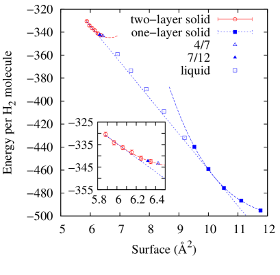
Figure 1: Energy per H₂ molecule as a function of the inverse of the total density of H₂ on graphite. The dotted line represent the Maxwell construction to determine the transition densities from a one-layer system to a two-layer arrangement. The curves are polynomial fits to the data and are intended only as guides-to-the-eye. The inset is a zoom on the two-layer solid energies.

III Results

The first relevant issue is establishing the stability limits of the different phases of H₂ adsorbed on graphite. This was done to ascertain whether there was any substantial difference with the phase diagram of the second layer of H₂ on graphene dealt with in Ref. yo2013, . To do so, we calculated the energies per molecule for the different arrangements we have considered, i.e., a first-layer triangular crystal and a second-layer with two possibilities: liquid and a triangular incommensurate solid on top of another triangular incommensurate solid in the first layer. As indicated above, those results are the average of at least 10 Monte Carlo histories for each density. To avoid spurious correlations, only values located 100 Monte Carlo steps away were used to obtain the mean energies. Our DMC results are shown in Fig. 1. The double-tangent Maxwell construction line indicates that one-layer incommensurate solid of 0.097 $\pm$ 0.002 Å^-2 is in equilibrium with two stacked triangular incommensurate crystals of total density 0.1650 $\pm$ 0.0025 Å^-2, as can be better seen in the inset of that figure. The density of the first layer was 0.100 Å^-2, density at which the total energy of the entire arrangement was found to be the lowest one. This density translates to a H₂-H₂ lattice constant of 3.4 Å. Those results are in good agreement with the ones for graphene yo2013 . Apart from the values of the equilibrium densities, the main features of Fig. 1 coincide with both the graphene calculation and available experimental data doble , i.e., there are no stable second-layer liquid nor registered commensurate solids of the second layer with respect the first one (either 4/7 or 7/12) since, in both cases, the energies are above the Maxwell line. A picture of those commensurate arrangements can be found in Refs. fukuyama, and kwon, , respectively.

The low mass of the H₂ molecule makes it a good candidate to exhibit macroscopic quantum behavior. To explore this possibility, we studied if we could find a supersolid phase within the stability range of the second-layer triangular solid. We chose H₂ on top of H₂, on top of graphite, because the supersolidity of the first layer had been ruled out in a previous calculation prb2011a . Following the same procedure as in Ref. B13, for ⁴He adsorbed on graphite, we estimated the superfluid fraction in two dimensions $\rho_{s}/\rho$ of H₂ in the second layer by using the zero-temperature winding number estimator,

$$\frac{\rho_{s}}{\rho}=\lim_{\tau\to\infty}\alpha\left(\frac{D_{s}(\tau)}{\tau}\right)\ ,$$ (7)

with $\tau$ the imaginary time used in the quantum Monte Carlo simulation. Here, $\alpha=N_{2}/(4D_{0})$, $D_{0}=\hbar^{2}/(2m)$, and $D_{s}(\tau)=\langle[{\bf R}_{CM}(\tau)-{\bf R}_{CM}(0)]^{2}\rangle$. ${\bf R}_{CM}$ is the position of the center of mass of the $N_{2}$ H₂ molecules located in the second layer. To perform those calculations, we took into account only their $x$ and $y$ coordinates, where periodic boundary conditions apply. The results obtained for a system with a total density of 0.1650 Å^-2 are displayed in Fig. 2. There, we show $\alpha D_{s}(\tau)$ vs. $\tau$, the superfluid fraction being the slope of the curve for $\tau\to\infty$. As one can see in Fig. 2, $\rho_{s}/\rho$ is noticeable different from zero, i.e., the system is a supersolid at that density.

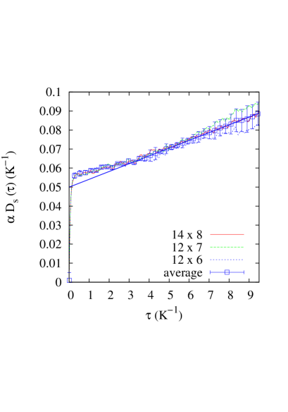
Figure 2: Estimator of the superfluid density for a total density $\rho$ = 0.1650 Å^-2 for different sizes of the simulation cell expressed as multiplets of a single unit cell in the first layer. Lines, simulation results; open squares, average of all the estimator for the three cells displayed. The straight line represent a linear least-squares fit to the the symbols displayed in the range (3 $<\tau<$ 8 K^-1). The slope of that curve implies a superfluid density of 0.41 $\pm$ 0.05 %.

To be sure that this result did not depend on our chosing of any particular setup, and to be sure that there were no influence of any possible sluggishness in the superfluid estimator, we performed DMC simulations using three different simulation cells. For instance, a 14 $\times$ 8 simulation cell is made of 14 first-layer unit cells in the $x$ direction, and of 8 of those unit cells in the $y$ direction. Since, as mentioned before, the distance between H₂ molecules in that first layer is 3.4 Å, this means a 47.6 $\times$ 47.11 Ų simulation cell. Conversely, the dimensions of a 12 $\times$ 6 cell are 40.8 $\times$ 35.33 Ų. This implies a surface ratio between both setups of $\sim$1.55. The superfluid estimator (7) was calculated as the average of ten statistically independent simulations and displayed in Fig. 2 as a thin line. No obvious size trend was found, the values for the three simulation cells being remarkably close to each other. In fact, the open squares in that figure represent the average of the three of them for each $\tau$, the error bars corresponding to two standard deviations of that average and including all the values obtained in the simulations.

To obtain the superfluid fraction, we performed a least-squares linear fitting procedure to the average of $\alpha D_{s}(\tau)$ vs. $\tau$ for the three simulation cells considered. The $\tau$ values were in the range 3 $<\tau<$8 K^-1. The result is displayed as the thick continuous line in Fig. 2. The procedure produces an slope, corresponding to the superfluid fraction, of 0.41 $\pm$ 0.05 %. If instead of using the average of $\alpha D_{s}(\tau)$ as an input in the fitting procedure, we consider the values for each simulation cell separately, we get superfluid fractions of 0.36 $\pm$ 0.05 % for the 12 $\times$ 6 cell, 0.48 $\pm$ 0.05 % for the 12 $\times$ 7 cell, and 0.39 $\pm$ 0.05 % for the 14 $\times$ 7 cell. Larger cells are beyond our calculating capabilities. These values are of the same order as the superfluid fraction obtained for the metastable, strictly 2D, systems considered in Ref. claudio . According to the results displayed in Fig. 1, the arrangement with a total density of 0.1650 Å^-2 is stable, and thus we can conclude that this supersolid could be observed. We can also see that the least-squares fit also describes well the interval $\tau>$ 8 K^-1, indicating that no further lengthening of the simulation series is necessary to obtain an accurate value of the superfluid fraction.

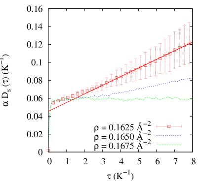
Figure 3: Same as in Fig. 2, but for different total densities and a fixed 14 $\times$ 8 simulation cell. The slope for the density $\rho$ = 0.1625 Å^-2 implies a superfluid fraction of 0.96 $\pm$ 0.05 %. Error bars are only shown for the lower density to make the figure more clear; for the other two densities they are of the same size.

To check the density range in which that supersolid phase could be stable, we calculated the superfluid fraction (Eq. 7) for total densities of 0.1625 Å^-2 (metastable) and 0.1675Å^-2. We did not consider the 4/7 and 7/12 unstable phases since their corresponding densities (0.157 and 0.158 Å^-2 respectively) are too far away from the stability region. The results are shown in Fig. 3 for a 14 $\times$ 8 simulation cell. We observe that, for the lower density, there is an appreciable superfluid fraction of 0.96$\pm$ 0.05 %. However, in the other case corresponding to the higher density, the slope of the estimator is zero, implying that the second layer of H₂ at that density is a normal solid.

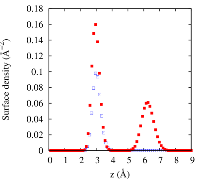
Figure 4: Density profile in the direction perpendicular to the graphite plane. Open squares, density corresponding to a first-layer commensurate $\sqrt{3}\times\sqrt{3}$ structure; full squares, a two-layer system of total density $\rho$ = 0.1650 Å^-2.

IV Conclusions

Summarizing, our microscopic quantum Monte Carlo approach shows that there is a narrow density slice around 0.1650 Å^-2 in which an incommensurate triangular second-layer H₂ supersolid is stable. We can try to understand the reasons behind this somehow unexpected result. The first ingredient is undoubtedly the low density of the crystal considered. That second-layer density is 0.0650 Å^-2. However, this is larger that the 0.060 Å^-2 upper density limit for which you can see a superfluid fraction in a pure 2D crystal claudio and also larger than the 0.0636Å^-2 first layer density for which no superfluid was found in Ref. prb2011a, . Therefore, an additional factor is needed. That factor can be understood with the help of Fig. 4. There, we show the density profile of a $\sqrt{3}\times\sqrt{3}$ first layer registered phase, together with the double layer supersolid arrangement in a direction perpendicular ($z$) to the graphite plane. What we can see is that there is an appreciable difference between the $z$-width of the first (bare or with H₂ on top) and second H₂ layers. In particular, the ratio between their widths, estimated considering the first- and second-layer profiles as Gaussians, is about 1.5. This implies a considerably larger leeway for the molecules in the second layer to move, and to allow for the exchanges needed to create a superfluid. That is corroborated by the superfluidity fraction of 0.58 $\pm$ 0.05 % obtained for a second layer of H₂ of the same density adsorbed on top of a first layer of D₂. The second-layer density profile in this case is virtually identical to the presented in Fig. 4 and not shown for simplicity. This means that the origin of this feature is in the transverse displacement of the molecules in the second layer.

The only remaining and crucial issue would be about the possibility of detecting such a small superfluid fraction. In a very recent experimental work kim , this is shown to be feasible for a double layer of ⁴He on top of graphite, since they were able to detect fractions as small as 0.9%. Importantly, the temperatures at which that behavior was seen in ⁴He are well below 0.5 K, what makes us confident that our zero-temperature DMC results for H₂ would hold in future experiments to come. Incidentaly, we should say that a very recent calculation parrinello points out to the existence of a supersolid in a quite different, but related system, bulk D₂ at very high pressures.

- (1) L.W. Bruch, M.W. Cole, and E. Zaremba. Physical Adsorption, Forces and Phenomena (Dover, New York, 1997).
- (2) D. S. Greywall and P. A. Busch, Phys. Rev. Lett. 67, 3535 (1991).
- (3) D. S. Greywall, Phys. Rev. B 47, 309 (1993).
- (4) G. Zimmerli, G. Mistura, and M. H. W. Chan, Phys. Rev. Lett. 68, 60 (1992).
- (5) P. A. Crowell and J. D. Reppy, Phys. Rev. Lett. 70, 3291 (1993).
- (6) P. A. Crowell and J. D. Reppy, Phys. Rev. B 53, 2701 (1996).
- (7) H. Freimuth and H. Wiechert, Surf. Sci. 162, 432 (1985).
- (8) H. Freimuth and H. Wiechert, Surf. Sci. 189/190, 548 (1987).
- (9) J. Ma, D. L. Kingsbury, F. C. Liu, and O. E. Vilches, Phys. Rev. Lett. 61, 2348 (1988). ,
- (10) J. Cui and S.C. Fain Jr., Phys. Rev. B. 39 8628 (1989).
- (11) H. Wiechert, in Excitations in Two-Dimensional and Three-Dimensional Quantum Fluids edited by A.G.F. Wyatt and H.J. Lauter (Plenum Press, New York, 1991). p. 499.
- (12) O.E. Vilches, J. Low Temp. Phys. 89, 267 (1992).
- (13) W. Liu and S.C. Fain Jr., Phys. Rev. B 47, 15965 (1993).
- (14) F. C. Liu, Y. M. Liu, and O. E. Vilches, Phys. Rev. B 51, 2848 (1995).
- (15) A. Noury, J. Vergara-Cruz, P. Morfin, B. Placais, M. C. Gordillo, J. Boronat, S. Balibar, and A. Bachtold, Phys. Rev. Lett 122, 165301 (2019).
- (16) Emin Menachekanian, Vito Iaia, Mingyu Fan, Jingjing Chen, Chaowei Hu, Ved Mittal, Gengming Liu, Raul Reyes, Fufang Wen, and Gary A. Williams Phys. Rev. B 99, 064503 (2019).
- (17) S. Nakamura, K. Matsui, T. Matsui, and H. Fukuyama, Phys. Rev. B 94, 180501(R) (2016).
- (18) J. Nyéki, A. Phillis, A. Ho, D. Lee, P. Coleman, J. Parpia, B. Cowan, and J. Saunders, Nature Phys. 13, 455 (2017).
- (19) Jaewon Choi, Alexey A. Zadorozhko, Jeakyung Choi, and Eunseong Kim, Phys. Rev. Lett. 127, 135301 (2021).
- (20) M. C. Gordillo and J. Boronat, Phys. Rev. Lett. 124, 205301 (2020).
- (21) M. C. Gordillo, C. Cazorla, and J. Boronat, Phys. Rev. B 83, 121406(R) (2011).
- (22) C. Cazorla and J. Boronat, Phys. Rev. B 78, 134509 (2008).
- (23) S. Grebenev, B. Sartakov, J. P. Toennies, and A. F. Vilesov, Science 289, 1532 (2000).
- (24) H. Li, R. J. Le Roy, P. N. Roy, and A. R. W. McKellar, Phys. Rev. Lett. 105, 133401 (2010).
- (25) P. Sindzingre, D. M. Ceperley, and M. L. Klein, Phys. Rev. Lett. 67, 1871 (1991).
- (26) M.C. Gordillo. Phys. Rev. B 60 6790 (1999).
- (27) M.C. Gordillo and D.M. Ceperley. Phys. Rev. B 65, 174527 (2002).
- (28) F. Mezzacapo and M. Boninsegni, Phys. Rev. Lett. 100, 145301 (2008).
- (29) E. Sola and J. Boronat, J. Phys. Chem. A 115, 7071 (2011).
- (30) Y. Kwon and K.B. Whaley. Phys. Rev. Lett. 89 273401 (2002).
- (31) O. N. Osychenko, R. Rota, and J. Boronat, Phys. Rev. B 85, 224513 (2012).
- (32) J. Léonard, A. Morales, P. Zupancic, T. Esslinger, and T. Donner, Nature (London) 543, 87 (2017),
- (33) J. Li, J. Lee, W. Huang, S. Burchesky, B. Shteynas, F. Top, A. Jamison, and W. Ketterle, Nature (London) 543, 91 (2017),
- (34) L. Tanzi, E. Lucioni, F. Fama, J. Catani, A. Fioretti, C. Gabbanini, R.N. Bisset, L. Santos, and G. Modugno, Phys. Rev. Lett. 122, 130405 (2019).
- (35) J. Boronat, in Microscopic Approaches to Quantum Liquids in Confined Geometries, Vol. 4, ed. E. Krotscheck and J. Navarro (World Scientific, Singapore, 2002).
- (36) G. Stan and M. W. Cole, J. Low Temp. Phys. 110, 539 (1998).
- (37) M. C. Gordillo and J. Boronat. Phys. Rev. B 87, 165403 (2013).
- (38) I. F. Silvera and V. V. Goldman, J. Chem. Phys. 69, 4209 (1978).
- (39) M.C. Gordillo and J. Boronat. Phys. Rev. B 81, 155435 (2010).
- (40) H. Fuyuyama. J. Phys. Soc. Japan 77 111013 (2008).
- (41) Y. Kwon and D.M. Ceperley. Phys. Rev. B 85 224501 (2012).
- (42) C. W. Myung ,B. Hirshberg, and M. Parrinello Phys. Rev. Lett. 128 045301 (2022).