A deep branching solver for fully nonlinear partial differential equations

Abstract

We present a multidimensional deep learning implementation of a stochastic branching algorithm for the numerical solution of fully nonlinear PDEs. This approach is designed to tackle functional nonlinearities involving gradient terms of any orders, by combining the use of neural networks with a Monte Carlo branching algorithm. In comparison with other deep learning PDE solvers, it also allows us to check the consistency of the learned neural network function. Numerical experiments presented show that this algorithm can outperform deep learning approaches based on backward stochastic differential equations or the Galerkin method, and provide solution estimates that are not obtained by those methods in fully nonlinear examples.

Keywords: Fully nonlinear PDE, deep neural network, deep Galerkin, deep BSDE, branching process, random tree, Monte Carlo method.

Mathematics Subject Classification (2020): 35G20, 35K55, 35K58, 60H30, 60J85, 65C05.

1 Introduction

This paper is concerned with the numerical solution of fully nonlinear partial differential equations (PDEs) of the form

$$\begin{cases}\displaystyle\partial_{t}u(t,x)+\frac{1}{2}\Delta u(t,x)+f\big{(}\partial_{\lambda^{1}}u(t,x),\ldots,\partial_{\lambda^{n}}u(t,x)\big{)}=0,\vskip 6.0pt plus 2.0pt minus 2.0pt\\ u(T,x)=\phi(x),\qquad(t,x)=(t,x_{1},\ldots,x_{d})\in[0,T]\times{}^{d},\end{cases}$$ (1.1)

$d\geq 1$, where $\Delta=\sum\limits_{i=1}^{d}\partial^{2}/\partial x^{2}_{i}$ is the standard $d$-dimensional Laplacian, $\partial_{t}u(t,x)=\partial u(t,x)/\partial t$, and $f$ is a smooth function of the derivatives

$$\partial_{\lambda^{i}}u(t,x)=\frac{\partial^{\lambda_{1}^{i}}}{\partial x_{1}}\cdots\frac{\partial^{\lambda_{d}^{i}}}{\partial x_{d}}u(t,x_{1},\ldots,x_{d}),\qquad(x_{1},\ldots,x_{d})\in{}^{d},$$

$\lambda^{i}=\left(\lambda^{i}_{1},\dots,\lambda^{i}_{d}\right)\in\mathbb{N}^{d}$, $i=1,\ldots,n$. As is well known, standard numerical schemes for solving (1.1) by e.g. finite differences or finite elements suffer from the curse of dimensionality as their computational cost grows exponentially with the dimension $d$.

The deep Galerkin method (DGM) has been developed in [SS18] for the numerical solution of (1.1) by training a neural network function $v(t,x)$ using the loss function

$$\left(\partial_{t}v(t,x)+\frac{1}{2}\Delta v(t,x)+f\big{(}\partial_{\lambda^{1}}v(t,x),\ldots,\partial_{\lambda^{n}}v(t,x)\big{)}\right)^{2}+\left(v(T,x)-\phi(x)\right)^{2}.$$ (1.2)

See [LZCC22] for recent improvements of the DGM using deep mixed residuals (MIM) with numerical applications to linear PDEs, and [HFH⁺22] for the blocked residual connection method (DLBR) applied to a linear (generalized) Black-Scholes equation.

On the other hand, probabilistic schemes provide a promising direction to overcome the curse of dimensionality. For example, when $f(u(t,x))=ru(t,x)$ does not involve any derivative of $u$, the solution of the PDE

$$\begin{cases}\displaystyle\partial_{t}u(t,x)+\frac{1}{2}\Delta u(t,x)+ru(t,x)=0,\vskip 6.0pt plus 2.0pt minus 2.0pt\\ u(T,x)=\phi(x),\qquad(t,x)=(t,x_{1},\ldots,x_{d})\in[0,T]\times{}^{d},\end{cases}$$

admits the probabilistic representation

$$u(0,x)=\mathrm{e}^{rT}\mathbb{E}[\phi(x+W_{T})],$$

where $(W_{t})_{t\geq 0}$ is a standard Brownian motion. This method can be implemented on a bounded domain $D\subset{}^{d}$ based on the universal approximation theorem and the $L^{2}$ minimality property

$$u(0,\cdot)=\inf\limits_{v}\mathbb{E}\big{[}\big{(}\mathrm{e}^{rT}\phi(X+W_{T})-v(X)\big{)}^{2}\big{]},$$

where $X$ is a uniform random vector on $D$ and the infimum in $v$ is taken over a neural functional space.

Probabilistic representations for the solutions of first order nonlinear PDEs can also be obtained by representing $u(t,x)$ as $u(t,x)=Y_{t}^{t,x}$, $(t,x)\in[0,T]\times\real$, where $(Y_{s}^{t,x})_{t\leq s\leq T}$ is the solution of a backward stochastic differential equation (BSDE), see [Pen91], [PP92]. The BSDE method has been implemented in [HJE18] using a deep learning algorithm in the case where $f$ depends on the first order derivative, i.e. $\lambda^{i}_{1}+\cdots+\lambda^{i}_{d}\leq 1$, $1\leq i\leq n$, see also [HPW20] for recent improvements. The BSDE method extends to second order fully nonlinear PDEs by the use of second order backward stochastic differential equations, see e.g. [CSTV07], [STZ12], and [HJE17, BEJ19], and [PWG21], [LLP23], for deep learning implementations. However, this approach does not apply to nonlinearities in gradients of order strictly greater than two, see Examples e) and f) below.

Numerical solutions of semilinear PDEs have also been obtained by the multilevel Picard method (MLP), see [EHJK19, HJKN20, EHJK21, HJK22], with numerical experiments provided in [BBH⁺20]. However, this approach is currently restricted to first order gradient nonlinearities, similarly to the deep splitting algorithm of [BBC⁺21]. In addition, the main use of the MLP and deep splitting methods is to provide pointwise estimates, whereas this paper focuses on functional estimation of solutions using neural networks.

In this context, the use of stochastic branching diffusion mechanisms [Sko64], [INW69], represents an alternative to the DGM and BSDE methods, see [McK75] for an application to the Kolmogorov-Petrovskii-Piskunov (KPP) equation, [CLM08] for existence of solutions of parabolic PDEs with power series nonlinearities, [HL12] for more general PDEs with polynomial nonlinearities, and [HLT21] for an application to semilinear and higher-order hyperbolic PDEs. This approach has been applied in e.g. [LM96], [HLOT⁺19] to polynomial gradient nonlinearities, see also [FTW11], [Tan13], [GZZ15], [HLZ20] for finite difference schemes combined with Monte Carlo estimation for fully nonlinear PDEs with gradients of order up to $2$.

Extending such approaches to nonlinearities involving gradients of order greater than two involves technical difficulties linked to the integrability of the Malliavin-type weights used in repeated integration by parts argument, see page 199 of [HLOT⁺19]. Such higher order nonlinearities are also not covered by multilevel Picard [BBH⁺20] and deep splitting [BBC⁺21] methods, or by BSDE methods [HJE18, BEJ19], which are limited to first and second order gradients, respectively.

In [NPP23], a stochastic branching method that carries information on (functional) nonlinearities along a random tree has been introduced, with the aim of providing Monte Carlo schemes for the numerical solution of fully nonlinear PDEs with gradients of arbitrary orders.

In this paper, we present a deep learning implementation of the method of [NPP23] using Monte Carlo sampling, the law of large numbers, and the universal approximation theorem. Our approach to the numerical solution of the PDE (1.1) is based on the following steps:

1. The solution of PDE (1.1) is written as the conditional expectation of a functional of a random coding tree via the fully nonlinear Feynman-Kac formula Theorem 1 in [NPP23], see (2.2) below.

2. The conditional expectation is approximated by a neural network function through the $L^{2}$-minimality property and the universal approximation theorem.

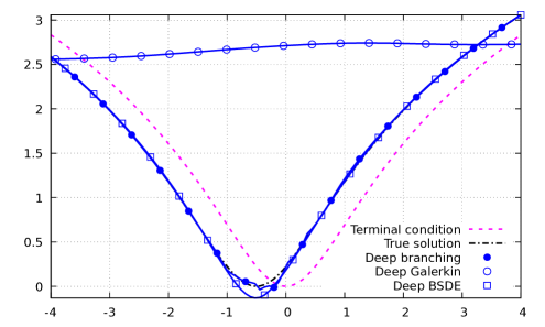
Figure 3: Comparison of deep learning methods for (4.2) with $d=5$ and $T=0.05$.

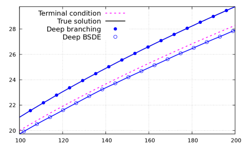
Figure 6: Deep branching vs deep BSDE method for (4.6) with $d=1$ and $T=0.1$.

We start by testing our method on the Allen-Cahn equation (4.1), for which we report a performance comparable to that of the deep BSDE and deep Galerkin methods, see Figure 2. This is followed by an example (4.2) involving an exponential nonlinearity without gradient term, in which our method outperforms the deep Galerkin method and performs comparably to deep BSDE method in dimension $d=5$, see Figure 3. We also consider a multidimensional Burgers equation (4.3) for which the deep branching method is more stable than the deep Galerkin and deep BSDE methods in dimension $d=15$, see Figure 5. Next, we consider a Merton problem (4.6) to which the deep Galerkin method does not apply since its loss function involves a division by the second derivative of the neural network function. We also note that the deep branching method overperforms the deep BSDE method in this case, see Figure 6. Finally, we consider higher order functional gradient nonlinearities in Equations (4.7) and (4.8), to which the deep BSDE, multilevel Picard and deep splitting methods do not apply. In those cases, our method also outperforms the deep Galerkin method in both dimensions $d=1$ and $d=5$, see Figures 8 and 9.

We also note that since the deep branching method is based on a direct Monte Carlo estimation, it allows for checking the consistency between the Monte Carlo samples and the learned neural network function, which is not possible with the deep Galerkin method and deep BSDE methods, see Figure 7.

Our algorithm, similarly to other branching diffusion methods, suffers from a time explosion phenomenon due to the use of a branching process. Nevertheless, our method can perform better than the deep Galerkin and deep BSDE methods in small time and in higher dimensions, see Figure 2 for the Allen-Cahn equation and Figure 5 for the Burgers equation.

Other approaches to the solution of evolution equations by carrying information on nonlinearities along trees include [But63], see also Chapters 4-6 of [DB02] and [MMMKV17] for ordinary differential equations (ODEs), with applications ranging from geometric numerical integration to stochastic differential equations, see for instance [HLW06] and references therein. On the other hand, the stochastic branching method does not use series truncations and it can be used to estimate an infinite series, see [PP22] for an application to ODEs.

This paper is organized as follows. The extension of the fully nonlinear Feynman-Kac formula of [NPP23] to a multidimensional setting is presented in Section 2, and the deep learning algorithm is described in Section 3. Section 4 presents numerical examples in which our method can outperform the deep BSDE and deep Galerkin methods.

The Python codes and numerical experiments run in this paper are available at

https://github.com/nguwijy/deep_branching.

Notation

We denote by $\mathbb{N}=\{0,1,2,\dots\}$ the set of natural numbers, and let $C^{0,\infty}([0,T]\times{}^{d})$ be the set of functions $u:[0,T]\times{}^{d}\to\real$ such that $u(t,x)$ is continuous in the variable $t$ and infinitely $x$-differentiable. For a vector $x=(x_{1},\ldots,x_{d})^{\top}\in{}^{d}$, we let $\lvert x\rvert=\sum\limits_{i=1}^{d}\lvert x_{i}\rvert$, and let $\bm{1}_{p}$ be the vector of $1$ at position $p$ and $0$ elsewhere. We also consider the linear order $\prec$ on ^d such that $(k_{1},\dots,k_{d})=k\prec l=(l_{1},\dots,l_{d})$ if one of the following holds:

1. $\lvert k\rvert<\lvert l\rvert$;

2. $\lvert k\rvert=\lvert l\rvert$ and $k_{1}<l_{1}$;

3. $\lvert k\rvert=\lvert l\rvert$, $k_{1}=l_{1},\dots k_{i}=l_{i}$, and $k_{i+1}<l_{i+1}$ for some $1\leq i<d$.

2 Fully nonlinear Feynman-Kac formula

In this section we extend the construction of [NPP23] to the case of multidimensional PDEs of the form

$$\begin{cases}\displaystyle\partial_{t}u(t,x)+\frac{1}{2}\Delta u(t,x)+f\big{(}\partial_{\lambda^{1}}u(t,x),\ldots,\partial_{\lambda^{n}}u(t,x)\big{)}=0,\vskip 6.0pt plus 2.0pt minus 2.0pt\\ u(T,x)=\phi(x),\qquad(t,x)=(t,x_{1},\ldots,x_{d})\in[0,T]\times{}^{d},\end{cases}$$ (2.1)

where $\lambda^{i}=\left(\lambda_{1}^{i},\ldots,\lambda_{d}^{i}\right)\in\mathbb{N}^{d}$, $i=1,\ldots,n$, with the integral formulation

$$u(t,x)=\int_{{}^{d}}\varphi(T-t,y-x)\phi(y)dy+\int_{t}^{T}\int_{{}^{d}}\varphi(s-t,y-x)f\big{(}\partial_{\lambda^{1}}u(t,y),\ldots,\partial_{\lambda^{n}}u(t,x)\big{)}dyds,$$

where $\varphi(t,x):=\mathrm{e}^{-x^{2}/(2t)}/{\sqrt{2\pi t}}$, and $(t,x)\in[0,T]\times{}^{d}$. We refer to e.g. Theorem 1.1 in [Kry83] for sufficient conditions for existence and uniqueness of smooth solutions to such fully nonlinear PDEs in the second order case. Our fully nonlinear Feynman-Kac formula [NPP23] relies on the construction of a branching coding tree, based on the definition of a set $\mathcal{C}$ of codes and its associated mechanism $\mathcal{M}$. In what follows, we use the notation

$$(a_{1},\ldots,a_{n})\cup(b_{1},\ldots,b_{m}):=(a_{1},\ldots,a_{n},b_{1},\ldots,b_{m})$$

for any sequences $(a_{1},\ldots,a_{n})$, $(b_{1},\ldots,b_{m})$ or real numbers. In addition, for any function $g:{}^{n}\to\real$, we let $g^{*}$ be the operator mapping $C^{0,\infty}([0,T]\times{}^{d})$ to $C^{0,\infty}([0,T]\times{}^{d})$ and defined by

$$g^{*}(u)(t,x):=g\big{(}\partial_{\lambda^{1}}u(t,x),\ldots,\partial_{\lambda^{n}}u(t,x)\big{)},\qquad(t,x)\in[0,T]\times{}^{d}.$$

In the sequel, we also let $\partial_{\lambda}:=\partial_{z_{1}}^{\lambda_{1}}\cdots\partial_{z_{n}}^{\lambda_{n}}$, and $\partial_{\mu}:=\partial_{x_{1}}^{\mu_{1}}\cdots\partial_{x_{d}}^{\mu_{d}}$, $\lambda=(\lambda_{1},\ldots,\lambda_{n})\in{\mathord{\mathbb{N}}}^{n}$, $\mu=(\mu_{1},\ldots,\mu_{d})\in{\mathord{\mathbb{N}}}^{d}$.

Definition 2.1

We let $\mathcal{C}$ denote the set of operators from ${\cal C}^{0,\infty}([0,T]\times{}^{d})$ to ${\cal C}^{0,\infty}([0,T]\times{}^{d})$, called codes, and defined as

$$\mathcal{C}:=\left\{{\rm Id},\ (a\partial_{\lambda}f)^{*},\ \partial_{\mu},\ :\ \lambda\in\mathbb{N}^{n},\ \mu\in\mathbb{N}^{d},\ a\in\real\right\},$$

where ${\rm Id}$ denotes the identity on ${\cal C}^{0,\infty}([0,T]\times{}^{d})$.

For example, for $\nu\in\mathbb{N}^{n}$, $\mu\in\mathbb{N}^{d}$, $a\in\real$ and $k\in\mathbb{N}$ we have

$$c(u)(T,x)=\begin{cases}\displaystyle\phi(x),&\text{if }c=\rm Id,\vskip 6.0pt plus 2.0pt minus 2.0pt\\ a\partial_{\nu}f\big{(}\partial_{\lambda^{1}}\phi(x),\ldots,\partial_{\lambda^{m}}\phi(x)\big{)},&\text{if }c=(a\partial_{\nu}f)^{*},\vskip 6.0pt plus 2.0pt minus 2.0pt\\ \partial_{\mu}\phi(x),&\text{if }c=\partial_{\mu}.\end{cases}$$

The mechanism $\mathcal{M}$ is then defined as a mapping on $\mathcal{C}$ by $\mathcal{M}({\rm Id}):=\{f^{*}\}$, and

$${\cal M}(g^{*}):=\bigcup_{1\leq p\leq n\atop\lambda^{p}=0}\big{\{}\big{(}f^{*},(\partial_{\bm{1}_{p}}g)^{*}\big{)}\big{\}}$$

$$\bigcup_{\footnotesize\begin{subarray}{c}1\leq p\leq n,\ 1\leq s\leq\lvert\lambda^{p}\rvert\\ 1\leq\nu_{1}+\cdots+\nu_{n}\leq\lvert\lambda^{p}\rvert\\ 1\leq\lvert k_{1}\rvert,\dots,\lvert k_{s}\rvert,\\ 0\prec l^{1}\prec\cdots\prec l^{s}\\ k^{i}_{1}+\cdots+k^{i}_{s}=\nu_{i},\ i=1,\dots,n\\ \lvert k_{1}\rvert l_{j}^{1}+\cdots+\lvert k_{s}\rvert l_{j}^{s}=\lambda^{p}_{j},\ j=1,\dots,d\end{subarray}}\left\{\left((\partial_{\bm{1}_{p}}g)^{*},\frac{\prod\limits_{i=1}^{d}\lambda^{p}_{i}!(\partial_{\nu}f)^{*}}{\prod\limits_{\footnotesize\begin{subarray}{c}1\leq r\leq s\\ 1\leq q\leq n\end{subarray}}k_{r}^{q}!\left(l_{1}^{r}!\cdots l_{d}^{r}!\right)^{k_{r}^{q}}}\right)\bigcup_{\footnotesize\begin{subarray}{c}1\leq r\leq s\\ 1\leq q\leq n\\ \end{subarray}}\big{(}\underbrace{\partial_{l^{r}+\lambda^{q}},\ldots,\partial_{l^{r}+\lambda^{q}}}_{k_{r}^{q}~{}{\rm times}}\big{)}\right\}$$

$$\qquad\qquad\quad\bigcup\bigcup_{\footnotesize\begin{subarray}{c}i,j=1,\dots,n\\ k=1,\dots,d\end{subarray}}\left\{\left(-\frac{1}{2}(\partial_{\bm{1}_{i}+\bm{1}_{j}}g)^{*},\partial_{\lambda^{i}+\bm{1}_{k}},\partial_{\lambda^{j}+\bm{1}_{k}}\right)\right\},\qquad g^{*}\in\mathcal{C},$$

and

$${\cal M}(\partial_{\mu})$$

$$:=\bigcup_{\footnotesize\begin{subarray}{c}1\leq s\leq\lvert\mu\rvert,\ 1\leq\nu_{1}+\cdots+\nu_{n}\leq\lvert\mu\rvert\\ 1\leq\lvert k_{1}\rvert,\dots,\lvert k_{s}\rvert,\ 0\prec l^{1}\prec\cdots\prec l^{s}\\ k^{i}_{1}+\cdots+k^{i}_{s}=\nu_{i},\ i=1,\dots,n\\ \lvert k_{1}\rvert l_{j}^{1}+\cdots+\lvert k_{s}\rvert l_{j}^{s}=\mu_{j},\ j=1,\dots,d\end{subarray}}\left\{\left(\frac{\prod\limits_{i=1}^{d}\mu_{i}!}{\prod\limits_{\footnotesize\begin{subarray}{c}1\leq r\leq s\\ 1\leq q\leq n\end{subarray}}k_{r}^{q}!\left(l_{1}^{r}!\cdots l_{d}^{r}!\right)^{k_{r}^{q}}}(\partial_{\nu}f)^{*}\right)\bigcup_{\footnotesize\begin{subarray}{c}1\leq r\leq s\\ 1\leq q\leq n\end{subarray}}\big{(}\underbrace{\partial_{l^{r}+\lambda^{q}}u,\ldots,\partial_{l^{r}+\lambda^{q}}u}_{k_{r}^{q}~{}{\rm times}}\big{)}\right\},$$

$\mu\in\mathbb{N}^{d}$. Given $\rho:{}_{+}\to(0,\infty)$ a probability density function (PDF) on ₊ with tail distribution function $\macc@depth\char 1\relax\frozen@everymath{\macc@group}\macc@set@skewchar\macc@nested@a 111{F}$ and $\mathcal{N}(0,\sigma^{2})$ a $d$-dimensional independent centered normal distribution with variance $\sigma^{2}$, we consider the functional $\mathcal{H}({t,x,c})$ constructed in Algorithm 1 along a random coded tree started at $(t,x,c)\in[0,T]\times{}^{d}\times{\cal C}$, using independent random samples on a probability space $\Omega$.

Algorithm 1 Coding tree algorithm TREE$(t,x,c)$

$t\in[0,T]$, $x\in{}^{d}$, $c\in\mathcal{C}$

$\mathcal{H}({t,x,c})\in\real$

$\mathcal{H}({t,x,c})\leftarrow 1$

$\tau\leftarrow$ a random variable drawn from the distribution of $\rho$

if $t+\tau>T$ then

     $W\leftarrow$ a random vector drawn from $\mathcal{N}(0,T-t)$

     $\mathcal{H}({t,x,c})\leftarrow\mathcal{H}({t,x,c})\times c(u)(T,x+W)/\macc@depth\char 1\relax\frozen@everymath{\macc@group}\macc@set@skewchar\macc@nested@a 111{F}(T-t)$

else

     $q\leftarrow$ the size of the mechanism set $\mathcal{M}(c)$

     $I\leftarrow$ a random element drawn uniformly from $\mathcal{M}(c)$

     $\mathcal{H}({t,x,c})\leftarrow\mathcal{H}({t,x,c})\times q/\rho(\tau)$

     for all $cc\in I$ do

         $W\leftarrow$ a random vector drawn from $\mathcal{N}(0,\tau)$

         $\mathcal{H}({t,x,c})\leftarrow\mathcal{H}({t,x,c})\times\text{TREE}(t+\tau,x+W,cc)$

     end for

end if

As in Theorem 1 in [NPP23], the following Feynman-Kac type identity

$$u(t,x)=\mathbb{E}[{\cal H}({t,x,\rm Id})]$$ (2.2)

for the solution of (1.1) holds under suitable integrability conditions on ${\cal H}({t,x,\rm Id})$ and smoothness assumptions on the coefficients of (1.1), see the appendix for calculation details.

3 Deep branching solver

Instead of evaluating (2.2) at a single point $(t,x)\in[0,T]\times{}^{d}$, we use the $L^{2}$-minimality property of expectation to perform a functional estimation of $u(\cdot,\cdot)$ as $u(\cdot,\cdot)=v^{*}(\cdot,\cdot)$ on the support of a random vector $(\tau,X)$ on $[0,T]\times{}^{d}$ such that $\mathcal{H}({\tau,X,\rm Id})\in L^{2}(\Omega)$, where

$$v^{*}=\operatorname*{arg\,min}\limits_{\{v\ \!:\ \!v(\tau,X)\in L^{2}\}}\mathbb{E}\left[\left(\mathcal{H}({\tau,X,\rm Id})-v(\tau,X)\right)^{2}\right].$$ (3.1)

To evaluate (2.2) on $[0,T]\times D$, where $D$ is a bounded domain of ^d, we can choose $(\tau,X)$ to be a uniform random vector on $[0,T]\times D$. Similarly, to evaluate (2.2) on $\{0\}\times D$, we may let $\tau\equiv 0$ and let $X$ be a uniform random vector on $D$.

In order to implement the deep learning approximation, we parametrize $v(\cdot,\cdot)$ in the functional space described below. Given $\sigma:\real\to\real$ an activation function such as $\sigma_{\rm ReLU}(x):=\max(0,x)$, $\sigma_{\tanh}(x):=\tanh(x)$ or $\sigma_{\rm Id}(x):=x$, we define the set of layer functions $\mathbb{L}^{\sigma}_{d_{1},d_{2}}$ by

$$\mathbb{L}^{\sigma}_{d_{1},d_{2}}:=\bigl{\{}L:{}^{d_{1}}\to{}^{d_{2}}\ :\ L(x)=\sigma(Ax+b),\ x\in{}^{d_{1}},\ A\in{}^{d_{2}\times d_{1}},\ b\in{}^{d_{2}}\bigr{\}},$$ (3.2)

where $d_{1}\geq 1$ is the input dimension, $d_{2}\geq 1$ is the output dimension, and the activation function $\sigma$ is applied component-wise to $Ax+b$. Similarly, when the input and output dimensions are the same, we define the set of residual layer functions $\mathbb{L}^{\rho,\rm res}_{d}$ by

$$\mathbb{L}^{\sigma,\rm res}_{d}:=\bigl{\{}L:{}^{d}\to{}^{d}\ :\ L(x)=x+\sigma(Ax+b),\ x\in{}^{d},\ A\in{}^{d\times d},\ b\in{}^{d}\bigr{\}},$$ (3.3)

see [HZRS16]. Then, we denote by

$$\mathbb{NN}^{\sigma,l,m}_{d}:=\bigl{\{}L_{l}\circ\dots\circ L_{0}:{}^{d}\to\real\ :\ L_{0}\in\mathbb{L}^{\sigma}_{d,m},\ L_{l}\in\mathbb{L}^{\sigma_{\rm Id}}_{m,1},\ L_{i}\in\mathbb{L}^{\sigma,\rm res}_{m},\ 1\leq i<l\bigr{\}}$$

the set of feed-forward neural networks with one output layer, $l\geq 1$ hidden residual layers each containing $m\geq 1$ neurons, where the activation functions of the output and hidden layers are respectively the identity function $\sigma_{\rm Id}$ and $\sigma$. Any $v(\cdot;\theta)\in\mathbb{NN}^{\sigma,l,m}_{d}$ is fully determined by the sequence

$$\theta:=\bigl{(}A_{0},b_{0},A_{1},b_{1},\dots,A_{l-1},b_{l-1},A_{l},b_{l}\bigr{)}$$

of $\left((d+1)m+(l-1)(m+1)m+(m+1)\right)$ parameters.

Since by the universal approximation theorem, see e.g. Theorem 1 of [Hor91], $\bigcup\limits_{m=1}^{\infty}\mathbb{NN}^{\sigma,l,m}_{d}$ is dense in the $L^{2}$ functional space, the optimization problem (3.1) can be approximated by

$$v^{*}\approx\operatorname*{arg\,min}\limits_{v\in\mathbb{NN}^{\sigma,l,m}_{d+1}}\mathbb{E}\left[\left(\mathcal{H}({\tau,X,\rm Id})-v(\tau,X)\right)^{2}\right].$$ (3.4)

By the law of large numbers, (3.4) can be further approximated by

$$v^{*}\approx\operatorname*{arg\,min}\limits_{v\in\mathbb{NN}^{\sigma,l,m}_{d+1}}N^{-1}\sum\limits_{i=1}^{N}\left(\mathcal{H}_{i}-v(\tau_{i},X_{i})\right)^{2},$$ (3.5)

where for all $i=1,\dots,N$, $(\tau_{i},X_{i})$ is drawn independently from the distribution of $(\tau,X)$ and $\mathcal{H}_{i}$ is drawn from $\mathcal{H}_{\tau_{i},X_{i},\rm Id}$ using Algorithm 1. However, the approximation (3.5) may perform poorly when the variance of $\mathcal{H}_{i}$ is too high. To solve this issue, we use the expression

$$v^{*}\approx\operatorname*{arg\,min}\limits_{v\in\mathbb{NN}^{\sigma,l,m}_{d+1}}N^{-1}\sum\limits_{i=1}^{N}\left(M^{-1}\sum\limits_{j=1}^{M}\mathcal{H}_{i,j}-v(\tau_{i},X_{i})\right)^{2},$$ (3.6)

where for $j=1,\dots,M$, $\mathcal{H}_{i,j}$ is drawn independently from $\mathcal{H}_{\tau_{i},X_{i},\rm Id}$ using Algorithm 1.

Finally, the deep branching method using the gradient descent method to solve the optimization in (3.6) is summarized in Algorithm 2.

Algorithm 2 Deep branching method

The learning rate $\eta$ and the number of epochs $P$

$v(\cdot,\cdot;\theta)\in\mathbb{NN}^{\sigma,l,m}_{d+1}$

$(\tau_{i},X_{i})_{1\leq i\leq N}\leftarrow$ random vectors drawn from the distribution of $(\tau,X)$

$(\mathcal{H}_{i,j})_{\footnotesize\begin{subarray}{c}1\leq i\leq N\\ 1\leq j\leq M\end{subarray}}\leftarrow$ random variables generated by TREE$(\tau_{i},X_{i},\rm Id)$ in Algorithm 1

Initialize $\theta$

for $i\leftarrow 1,\dots,P$ do

     $L\leftarrow N^{-1}\sum\limits_{i=1}^{N}\bigg{(}M^{-1}\sum\limits_{j=1}^{M}\mathcal{H}_{i,j}-v(\tau_{i},X_{i};\theta)\bigg{)}^{2}$

     $\theta\leftarrow\theta-\eta\nabla_{\theta}L$

end for

Remark 3.1

In the implementation of Algorithm 2, we perform the following additional steps:

1. $\eta\leftarrow\eta/10$ after every $\lfloor P/3\rfloor$ steps.

2. Instead of using $\eta$ to update $\theta$ directly, Adam algorithm is used to update $\theta$, see [KB14].

3. $\sigma_{\tanh}$ is used because the target PDE solution (1.1) is smooth.

4. A batch normalization layer is added after the activation function in (3.2)-(3.3) when $\sigma\neq\sigma_{\rm Id}$, see [IS15].

5. $\rho$ is chosen to be the PDF of exponential distribution with rate $-(\log 0.95)/T$.

6. Given $x_{\rm min}<x_{\rm max}$ and $x_{\rm mid}=(x_{\rm min}+x_{\rm max})/2$, we take

   $$D:=[x_{\rm min},x_{\rm max}]\times\{x_{\rm mid}\}\times\dots\times\{x_{\rm mid}\},$$

   and we let $(\tau,X)$ be the uniform random vector on $\{0\}\times D$.

4 Numerical examples

The numerical examples below are run in Python using PyTorch with the default initialization scheme for $\theta$, and the default values $N=1000$, $P=3000$, $\eta=0.01$, $l=6$, $m=20$. Except if otherwise stated, runtimes are expressed in minutes and the examples have been run on Google Colab with a Tesla P100 GPU.

For comparisons with the deep BSDE and deep Galerkin methods, we select the configurations such that all methods have comparable or similar runtimes. For the deep BSDE method of [HJE18, BEJ19], the time discretization of $(0,{T}/{5},{2T}/{5},{3T}/{5},{4T}/{5},T)$ and $1000$ (resp. $100,000$) number of samples are used in the case of $d=1$ (resp. $d>1$).

For the deep Galerkin method of [SS18], $10,000$ samples are respectively generated on $\{0\}\times[x_{\rm min},x_{\rm max}]^{d}$, $(0,T)\times[x_{\rm min},x_{\rm max}]^{d}$, and $\{T\}\times[x_{\rm min},x_{\rm max}]^{d}$. In our experiment, such generation works better than generating $10,000$ samples respectively on $\{0\}\times D$, $(0,T)\times D$, and $\{T\}\times D$. In addition, we found that batch normalization and learning rate decay in Remark 3.1 do not work well with deep Galerkin method, hence they are not used in the simulation below for the deep Galerkin method. The learning rate for the deep Galerkin method is fixed to be $\eta=0.001$ throughout the training.

The analysis of error is performed on the grid of $\widetilde{D}=(0,x_{\rm min}+i\Delta_{x},x_{\rm mid},\dots,x_{\rm mid})_{0\leq i\leq 100}$, where $\Delta_{x}=(x_{\rm max}-x_{\rm min})/100$. In each of the $10$ independent runs, the statistics of the runtime (in seconds) and the $L^{p}$ error $100^{-1}\sum\limits_{x\in\widetilde{D}}\lvert{\rm true}(x)-{\rm predicted}(x)\rvert^{p}$ are recorded. In multidimensional examples with $d\geq 2$, every figure is plotted as a function of $x_{1}$ on the horizontal axis, after setting $(x_{2},\ldots,x_{d})=(0,\ldots,0)$.

a) Allen-Cahn equation

Consider the equation

$$\partial_{t}u(t,x)+\frac{1}{2}\Delta u(t,x)+u(t,x)-u^{3}(t,x)=0,$$ (4.1)

which admits the traveling wave solution

$$u(t,x)=-\frac{1}{2}-\frac{1}{2}\tanh\left(\frac{3}{4}(T-t)-\sum\limits_{i=1}^{d}\frac{x_{i}}{2\sqrt{d}}\right),\qquad(t,x)\in[0,T]\times{}^{d}.$$

Table 1 summarizes the results of $10$ independent runs, with $M=100,000$, $T=0.5$, $x_{\rm min}=-8$, and $x_{\rm max}=8$.

Method	$d$	Mean $L^{1}$-error	Stdev $L^{1}$-error	Mean $L^{2}$-error	Stdev $L^{2}$-error	Mean Runtime
Deep branching	1	1.32E-03	1.05E-04	4.04E-06	7.32E-07	28m
Deep BSDE [HJE18]	1	4.60E-03	9.82E-04	4.08E-05	2.18E-05	101m
Deep Galerkin [SS18]	1	1.40E-03	1.83E-03	6.39E-06	1.57E-05	53m
Deep branching	5	3.63E-03	1.57E-04	2.09E-05	1.19E-06	110m
Deep BSDE [HJE18]	5	4.71E-03	4.23E-04	3.51E-05	8.19E-06	170m
Deep Galerkin [SS18]	5	6.83E-03	6.17E-03	1.36E-04	2.77E-04	134m

Table 1: Summary of numerical results for (4.1).

We check in Table 1 and Figure 1 that all three algorithms show a similar accuracy for the numerical solution of the Allen-Cahn equation, while the deep branching method appears more stable.

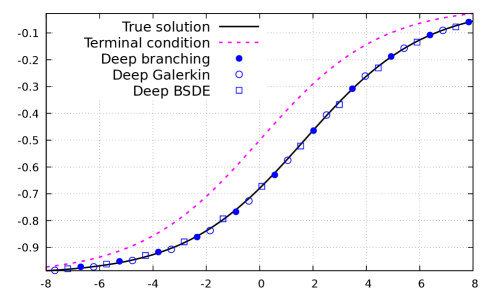
Figure 1: Comparison of deep learning methods for (4.1) with $d=5$ and $T=0.5$.

Figure 2 compares the $L^{1}$ errors of deep learning methods, showing that although the deep branching method has an explosive behavior, under comparable runtimes it can perform better than the deep Galerkin and deep BSDE methods in small time, in both dimensions $d=1$ and $10$. Figure 2 and Table 2 have been run on a RTX A4000 GPU.

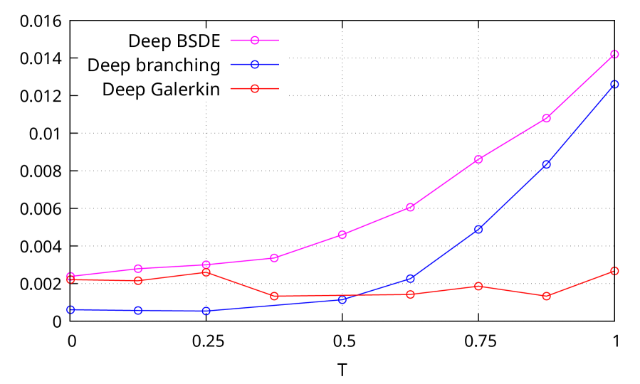
(a) Dimension $d=1$.

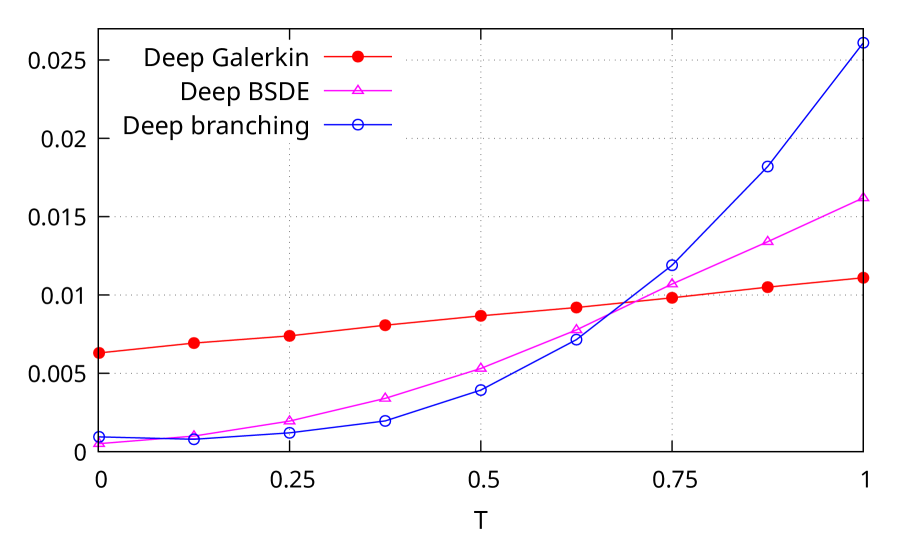
(b) Dimension $d=10$.

Figure 2: $L^{1}$ error graphs for (4.1) as functions of time $T$.

Table 2 ensures that the experiments of Figure 2 are performed within comparable runtimes.

Method	$d=1$	$d=10$
Deep branching	38m	279m
Deep Galerkin [HJE18]	69m	254m
Deep BSDE [SS18]	87m	237m

Table 2: Average runtimes in minutes for Figure 2.

b) Exponential nonlinearity

Consider the equation

$$\partial_{t}u(t,x)+\frac{\alpha}{d}\sum\limits_{i=1}^{d}\partial_{x_{i}}u(t,x)+\frac{1}{2}\Delta u(t,x)+\mathrm{e}^{-u(t,x)}(1-2\mathrm{e}^{-u(t,x)})d=0,$$ (4.2)

which admits the traveling wave solution

$$u(t,x)=\log\left(1+\left(\sum\limits_{i=1}^{d}x_{i}+\alpha(T-t)\right)^{2}\right),\qquad(t,x)\in[0,T]\times{}^{d}.$$

Table 3 summarizes the results of $10$ independent runs, with $M=30,000$ (resp. $M=3,000$) in dimension $d=1$ (resp. $d=5$), $\alpha=10$, $T=0.05$, $x_{\rm min}=-4$, and $x_{\rm max}=4$.

Method	$d$	Mean $L^{1}$-error	Stdev $L^{1}$-error	Mean $L^{2}$-error	Stdev $L^{2}$-error	Mean Runtime
Deep branching	1	1.17E-02	1.36E-03	4.57E-04	1.32E-04	42m
Deep BSDE [HJE18]	1	1.39E-02	2.26E-03	3.56E-04	1.03E-04	101m
Deep Galerkin [SS18]	1	2.53E-02	2.12E-02	1.72E-03	3.02E-03	61m
Deep branching	5	2.63E-02	4.53E-03	2.69E-03	1.08E-03	146m
Deep BSDE [HJE18]	5	1.88E-02	4.57E-04	1.36E-03	9.86E-05	119m
Deep Galerkin [SS18]	5	1.32E+00	7.78E-01	3.26E+00	2.54E+00	154m

Table 3: Summary of numerical results for (4.2).

In the case of exponential nonlinearity, our method appears significantly more accurate than the deep Galerkin method, and performs comparably to the deep BSDE method in dimension $d=5$.

c) Burgers equation

Next, we consider the multidimensional Burgers equation

$$\partial_{t}u(t,x)+\frac{d^{2}}{2}\Delta u(t,x)+\left(u(t,x)-\frac{2+d}{2d}\right)\left(d\sum_{k=1}^{d}\partial_{x_{k}}u(t,x)\right)=0,$$ (4.3)

with traveling wave solution

$$u(t,x)=\frac{\exp\big{(}t+d^{-1}\sum_{i=1}^{d}x_{i}\big{)}}{1+\exp\big{(}t+d^{-1}\sum_{i=1}^{d}x_{i}\big{)}},\qquad x=(x_{1},\ldots,x_{d})\in{}^{d},\ t\in[0,T],$$ (4.4)

see § 4.5 of [HJE17], and § 4.2 of [Cha13]. Figure 4 presents estimates of the solution of the Burgers equation (4.3) with solution (4.4) in dimensions $d=5$ and $d=20$, with comparisons to the outputs of the deep Galerkin method [SS18] and of the deep BSDE method [HJE18].

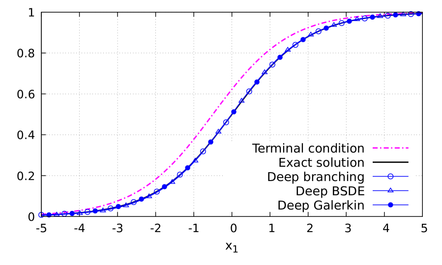
(a) Dimension $d=1$ with $T=0.5$.

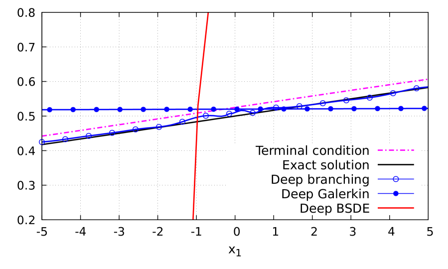
(b) Dimension $d=15$ with $T=0.1$.

Figure 4: Numerical solution of (4.3) and comparison to (4.4) with $\nu=d^{2}$.

We note in Figure 4$-b)$ that the deep branching method is more stable than the deep Galerkin and deep BSDE methods in dimension $d=15$. In particular, the deep BSDE estimate explodes under comparable runtimes, as shown in Figure 5. Figure 5 and Table 4 have been run on a RTX A4000 GPU.

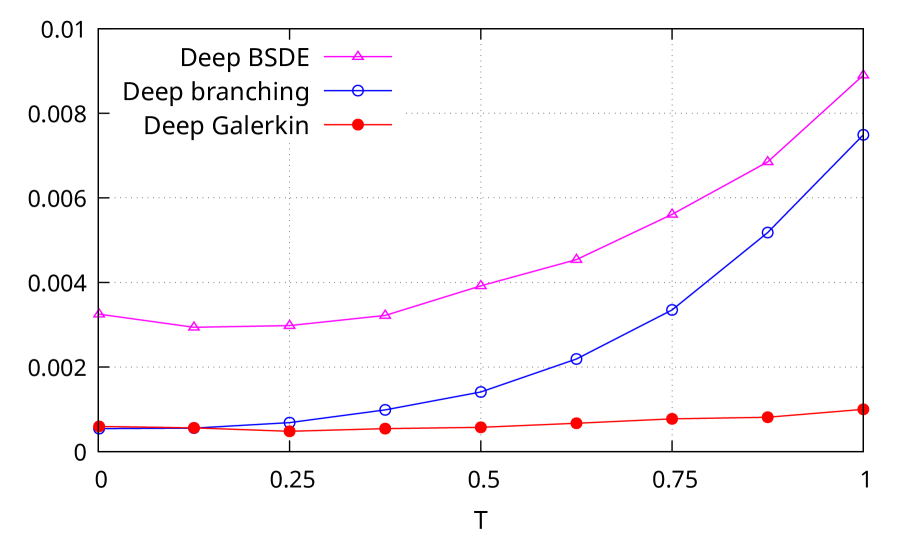
(a) Dimension $d=1$.

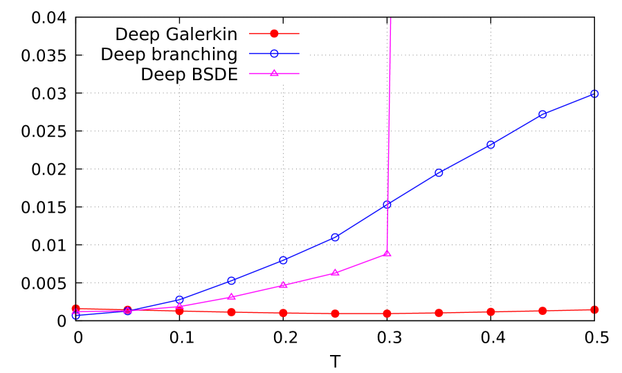
(b) Dimension $d=5$.

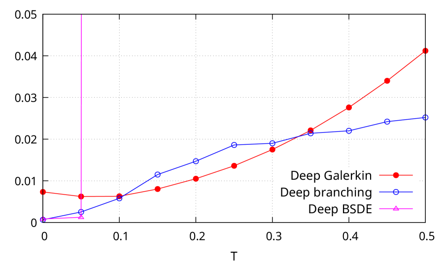
(c) Dimension $d=10$.

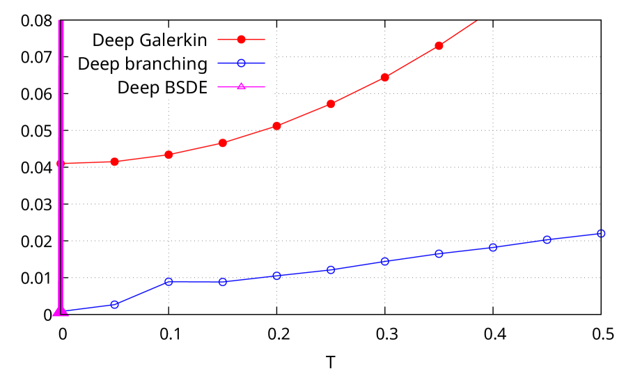
(d) Dimension $d=15$.

Figure 5: $L^{1}$ error graphs for the solution of (4.3) as functions of time $T$.

Table 4 ensures that the experiments of Figure 5 are performed within comparable runtimes.

Method	$d=1$	$d=5$	$d=10$	$d=15$
Deep branching	61m	72m	117m	169m
Deep Galerkin [HJE18]	77m	184m	331m	480m
Deep BSDE [SS18]	144m	146m	145m	124m

Table 4: Average runtimes in minutes for Figure 5.

d) Merton problem

Let $(X_{s})_{t\in[0,T]}$ be the solution of the controlled SDE

$$dX_{s}=(\mu\pi_{s}X_{s}-c_{s})ds+\pi_{s}\sigma X_{s}dB_{s}$$

started at $X_{t}=x$, where $(c_{s})_{s\in[0,T]}$ and $(\sigma_{s})_{s\in[0,T]}$ are square-integrable adapted processes. We consider the Merton problem

$$u(t,x)=\inf\limits_{(\pi_{s})_{t\leq s\leq T},\ \!(c_{s})_{t\leq s\leq T}}\mathbb{E}\left[\frac{e^{-\rho(T-t)}X_{T}^{1-\gamma}}{1-\gamma}+\int_{t}^{T}\frac{e^{-\rho(s-t)}c_{s}^{1-\gamma}}{1-\gamma}ds\right],$$ (4.5)

where $\gamma\in(0,1)$. The solution $u(t,x)$ of (4.5) satisfies the Hamilton-Jacobi-Bellman (HJB) equation

$$\partial_{t}u(t,x)+\sup\limits_{\pi,c}\left((\pi\mu x-c)\partial_{x}u(t,x)+\frac{\pi^{2}\sigma^{2}x^{2}}{2}\partial^{2}_{x}u(t,x)+\frac{c^{1-\gamma}}{1-\gamma}\right)=\rho u(t,x),$$

which, by first order condition, can be rewritten as

$$\partial_{t}u(t,x)-\frac{(\mu\partial_{x}u(t,x))^{2}}{2\sigma^{2}\partial^{2}_{x}u(t,x)}+\frac{\gamma}{1-\gamma}(\partial_{x}u(t,x))^{1-1/\gamma}=\rho u(t,x),$$ (4.6)

and admits the solution

$$u(t,x)=\frac{x^{1-\gamma}(1+(\alpha-1)e^{-\alpha(T-t)})^{\gamma}}{\alpha^{\gamma}(1-\gamma)},\qquad(t,x)\in[0,T]\times\real,$$

where $\alpha:=(2\sigma^{2}\gamma\rho-(1-\gamma)\mu^{2})/(2\sigma^{2}\gamma^{2})$. As the loss function used in the deep Galerkin method uses a division by the second derivatives of the neural network function, see (1.2) and (4.6), it explodes when the second derivatives of the learned neural network function becomes small during the training. Hence, in Table 5, we only present the outputs of the deep branching method and of the deep BSDE method of [BEJ19] which deals with second order gradient nonlinearities. Table 5 summarizes the results of $10$ independent runs, with $\mu=0.03$, $\sigma=0.1$, $\gamma=0.5$, $\rho=0.01$, $T=0.1$ on the interval $[x_{\rm min},x_{\rm max}]=[100,200]$, where we take $M=10,000$ in the deep branching method.

Method	$d$	Mean $L^{1}$-error	Stdev $L^{1}$-error	Mean $L^{2}$-error	Stdev $L^{2}$-error	Mean Runtime
Deep branching	1	8.49E-03	7.44E-04	1.30E-04	2.52E-05	54m
Deep BSDE [HJE18]	1	1.61E+00	1.05E-01	2.64E+00	3.37E-01	184m

Table 5: Summary of numerical results for (4.6).

An anomaly was detected on the third run when using $\sigma=\sigma_{\tanh}$, and it disappeared after changing the activation function to $\sigma=\sigma_{\rm ReLU}$.

In Figure 7, we plot the Monte Carlo samples generated by Algorithm 1 and the learned neural network function $v(\cdot,\cdot;\theta)$, see Algorithm 2, for $\sigma=\sigma_{\rm ReLU}$ and for $\sigma=\sigma_{\tanh}$ on the third run.

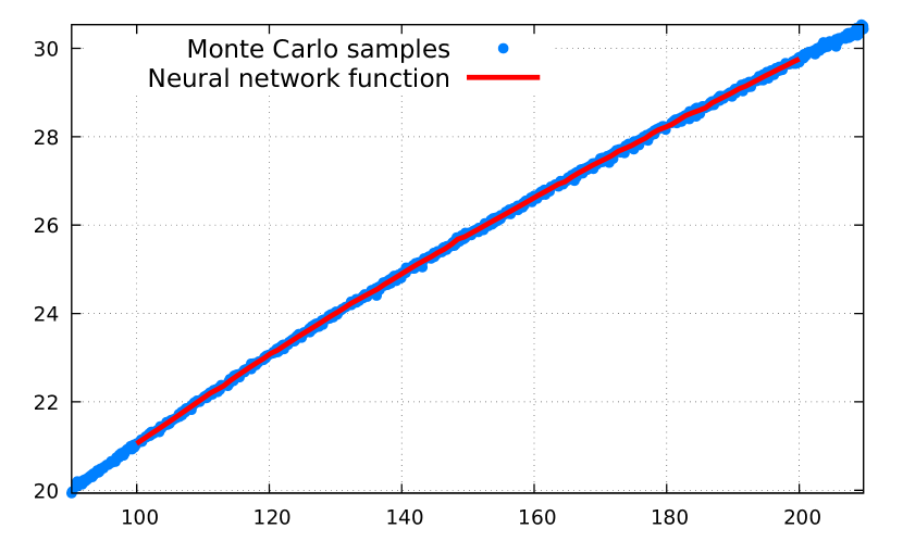
(a) $\sigma=\sigma_{\rm ReLU}$

(b) $\sigma=\sigma_{\tanh}$

Figure 7: Monte Carlo samples and the neural network function on the third run.

Figure 7 shows the consistency, or lack thereof, between the Monte Carlo samples and the learned neural network function, which cannot be observed when using the deep Galerkin or deep BSDE method.

e) Third order gradient log nonlinearity

This Example $e)$ and the next Example $f)$ use nonlinearities in terms of third and fourth order gradients, to which the deep BSDE method does not apply. For this reason, comparisons are done only with respect to the Galerkin method. Consider the equation

$$\partial_{t}u(t,x)+\frac{\alpha}{d}\sum\limits_{i=1}^{d}\partial_{x_{i}}u(t,x)+\log\left(\frac{1}{d}\sum\limits_{i=1}^{d}\left(\partial^{2}_{x_{i}}u(t,x)\right)^{2}+\left(\partial^{3}_{x_{i}}u(t,x)\right)^{2}\right)=0,$$ (4.7)

which admits the solution

$$u(t,x)=\cos\left(\sum\limits_{i=1}^{d}x_{i}+\alpha(T-t)\right),\qquad(t,x)\in[0,T]\times{}^{d}.$$

Table 6 summarizes the results of $10$ independent runs, with $M=6,000$ in dimension $d=1$ (resp. $M=200$ in dimension $d=5$), $\alpha=10$, $T=0.02$, $x_{\rm min}=-3$, and $x_{\rm max}=3$.

Method	$d$	Mean $L^{1}$-error	Stdev $L^{1}$-error	Mean $L^{2}$-error	Stdev $L^{2}$-error	Mean Runtime
Deep branching	1	5.82E-03	1.27E-03	5.52E-05	2.01E-05	78m
Deep Galerkin [SS18]	1	7.50E-02	3.15E-02	9.00E-03	7.34E-03	83m
Deep branching	5	2.77E-02	1.13E-02	3.52E-03	4.65E-03	183m
Deep Galerkin [SS18]	5	6.38E-01	5.74E-03	5.18E-01	1.08E-02	369

Table 6: Summary of numerical results for (4.7).

In the case of log nonlinearity with a third order gradient term, our method appears more accurate than the deep Galerkin method in dimensions $d=1$ and $d=5$. Figure 8 presents a numerical comparison on the average performance of 10 runs.

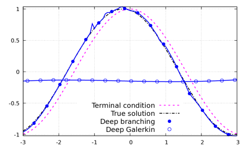
Figure 8: Deep branching vs deep Galerkin method for (4.7) with $d=5$ and $T=0.02$.

f) Fourth order gradient cosine nonlinearity

Consider the equation

$$\partial_{t}u(t,x)+\frac{\alpha}{d}\sum\limits_{i=1}^{d}\partial_{x_{i}}u(t,x)+u(t,x)-\left(\frac{\Delta u(t,x)}{12d}\right)^{2}+\frac{1}{d}\sum\limits_{i=1}^{d}\cos\left(\frac{\pi\partial^{4}_{x_{i}}u(t,x)}{4!}\right)=0,$$ (4.8)

which admits the solution

$$u(t,x)=\varphi\left(\sum\limits_{i=1}^{d}x_{i}+\alpha(T-t)\right),\qquad(t,x)\in[0,T]\times{}^{d},$$

where $\varphi(y):=y^{4}+y^{3}+by^{2}+cy+d$ for $y\in\real$, $b=-36/47$, $c=24b$, $d=4b^{2}$, and $\alpha=10$.

Table 7 summarizes the results of $10$ independent runs, with $M=2,500$ in dimension $d=1$ (resp. $M=50$ in dimension $d=5$), $\alpha=10$, $T=0.04$, $x_{\rm min}=-5$, and $x_{\rm max}=5$.

Method	$d$	Mean $L^{1}$-error	Stdev $L^{1}$-error	Mean $L^{2}$-error	Stdev $L^{2}$-error	Mean Runtime
Deep branching	1	9.62E+00	1.50E+00	3.76E+02	1.62E+02	128m
Deep Galerkin [SS18]	1	2.81E+01	2.77E+01	2.31E+03	4.45E+03	146m
Deep branching	5	1.01E+01	1.16E+00	3.49E+02	1.62E+02	259m
Deep Galerkin [SS18]	5	2.57E+02	1.18E+00	7.75E+04	6.55E+02	670

Table 7: Summary of numerical results for (4.8).

In the case of cosine nonlinearity with a fourth order gradient, our method appears more accurate than the deep Galerkin methods in dimensions $d=1$ and $d=5$. Figure 9 presents a numerical comparison on the average performance of 10 runs.

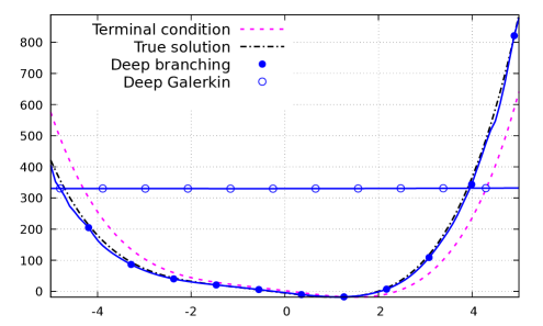
Figure 9: Deep branching vs deep Galerkin method for (4.8) with $d=5$ and $T=0.04$.

Appendix A Multidimensional extension

In this section we sketch the argument extending Theorem 1 in [NPP23] to the multidimensional case, and leading to (2.2). For this, given $g\in C^{0,\infty}([0,T]\times{}^{d})$ and $\mu\in{\mathord{\mathbb{N}}}^{n}$ such that $|\mu|\geq 1$, we will use the multivariate Faà di Bruno formula

$$\partial_{\mu}g^{*}(u)(t,x)=\left(\prod_{i=1}^{d}\mu_{i}!\right)\sum\limits_{\begin{subarray}{c}1\leq\nu_{1}+\cdots+\nu_{n}\leq\lvert\mu\rvert\\ 1\leq s\leq\lvert\mu\rvert\end{subarray}}(\partial_{\nu}g)^{*}(u)(t,x)\hskip-15.36429pt\sum\limits_{\begin{subarray}{c}1\leq\lvert k_{1}\rvert,\dots,\lvert k_{s}\rvert,\ 0\prec l^{1}\prec\cdots\prec l^{s}\\ k^{i}_{1}+\cdots+k^{i}_{s}=\nu_{i},\ i=1,\dots,n\\ \lvert k_{1}\rvert l_{j}^{1}+\cdots+\lvert k_{s}\rvert l_{j}^{s}=\mu_{j},\ j=1,\dots,d\end{subarray}}\prod_{\begin{subarray}{c}1\leq r\leq s\\ 1\leq q\leq n\end{subarray}}\frac{(\partial_{l^{r}+\lambda^{q}}u(t,x))^{k_{r}^{q}}}{k_{r}^{q}!\left(l_{1}^{r}!\cdots l_{d}^{r}!\right)^{k_{r}^{q}}},$$ (A.1)

see Theorem 2.1 in [CS96], applied to the function $g^{*}(u)(t,x):=g\big{(}\partial_{\lambda^{1}}u(t,x),\ldots,\partial_{\lambda^{n}}u(t,x)\big{)}$.

We have

$$\partial_{t}g^{*}(u)+\frac{1}{2}\Delta g^{*}(u)$$

$$= \sum\limits_{p=1}^{n}\partial_{\lambda^{p}}\left(\partial_{t}u+\frac{1}{2}\Delta u\right)(\partial_{\bm{1}_{p}}g)^{*}(u)+\frac{1}{2}\sum\limits_{i=1}^{n}\sum\limits_{j=1}^{n}\sum\limits_{k=1}^{d}\left(\partial_{\lambda^{i}+\bm{1}_{k}}u\right)\left(\partial_{\lambda^{j}+\bm{1}_{k}}u\right)(\partial_{\bm{1}_{i}+\bm{1}_{j}}g)^{*}(u)$$

$$= -\sum\limits_{p=1}^{n}(\partial_{\bm{1}_{p}}g)^{*}(u)\partial_{\lambda^{p}}f^{*}(u)+\frac{1}{2}\sum\limits_{i=1}^{n}\sum\limits_{j=1}^{n}\sum\limits_{k=1}^{d}\left(\partial_{\lambda^{i}+\bm{1}_{k}}u\right)\left(\partial_{\lambda^{j}+\bm{1}_{k}}u\right)(\partial_{\bm{1}_{i}+\bm{1}_{j}}g)^{*}(u)$$

$$= -\sum\limits_{p=1}^{n}\bm{1}_{\{\lambda^{p}=0\}}(\partial_{\bm{1}_{p}}g)^{*}(u)f^{*}(u)$$

$$-\sum\limits_{p=1}^{n}(\partial_{\bm{1}_{p}}g)^{*}(u)\left(\prod_{i=1}^{d}\lambda^{p}_{i}!\right)\sum\limits_{\begin{subarray}{c}1\leq\nu_{1}+\cdots+\nu_{n}\leq\lvert\lambda^{p}\rvert\\ 1\leq s\leq\lvert\lambda^{p}\rvert\end{subarray}}(\partial_{\nu}f)^{*}(u)\sum\limits_{\begin{subarray}{c}1\leq\lvert k_{1}\rvert,\dots,\lvert k_{s}\rvert,\ 0\prec l^{1}\prec\cdots\prec l^{s}\\ k^{i}_{1}+\cdots+k^{i}_{s}=\nu_{i},\ i=1,\dots,n\\ \lvert k_{1}\rvert l_{j}^{1}+\cdots+\lvert k_{s}\rvert l_{j}^{s}=\lambda^{p}_{j},\ j=1,\dots,d\end{subarray}}\prod_{\begin{subarray}{c}1\leq r\leq s\\ 1\leq q\leq n\end{subarray}}\frac{(\partial_{l^{r}+\lambda^{q}}u)^{k_{r}^{q}}}{k_{r}^{q}!\left(l_{1}^{r}!\cdots l_{d}^{r}!\right)^{k_{r}^{q}}}$$

$$\qquad\qquad\qquad+\frac{1}{2}\sum\limits_{i=1}^{n}\sum\limits_{j=1}^{n}\sum\limits_{k=1}^{d}\left(\partial_{\lambda^{i}+\bm{1}_{k}}u\right)\left(\partial_{\lambda^{j}+\bm{1}_{k}}u\right)(\partial_{\bm{1}_{i}+\bm{1}_{j}}g)^{*}(u).$$

Rewriting the above equation in integral form yields

$$g^{*}(u)(t,x)=\int_{{}^{d}}\varphi(T-t,y-x)g(\phi(y))dy$$

$$+\int_{t}^{T}\int_{{}^{d}}\varphi(s-t,y-x)$$

$$\biggl{(}\sum\limits_{p=1}^{n}\bm{1}_{\{\lambda^{p}=0\}}(\partial_{\bm{1}_{p}}g)^{*}(u)f^{*}(u)-\frac{1}{2}\sum\limits_{i=1}^{n}\sum\limits_{j=1}^{n}\sum\limits_{k=1}^{d}\left(\partial_{\lambda^{i}+\bm{1}_{k}}u(s,y)\right)\left(\partial_{\lambda^{j}+\bm{1}_{k}}u(s,y)\right)(\partial_{\bm{1}_{i}+\bm{1}_{j}}g)^{*}(u)$$

$$+\sum\limits_{p=1}^{n}(\partial_{\bm{1}_{p}}g)^{*}(u)\left(\prod_{i=1}^{d}\lambda^{p}_{i}!\right)\sum\limits_{\begin{subarray}{c}1\leq\nu_{1}+\cdots+\nu_{n}\leq\lvert\lambda^{p}\rvert\\ 1\leq s\leq\lvert\lambda^{p}\rvert\end{subarray}}(\partial_{\nu}f)^{*}(u)\sum\limits_{\begin{subarray}{c}1\leq\lvert k_{1}\rvert,\dots,\lvert k_{s}\rvert,\ 0\prec l^{1}\prec\cdots\prec l^{s}\\ k^{i}_{1}+\cdots+k^{i}_{s}=\nu_{i},\ i=1,\dots,n\\ \lvert k_{1}\rvert l_{j}^{1}+\cdots+\lvert k_{s}\rvert l_{j}^{s}=\lambda^{p}_{j},\ j=1,\dots,d\end{subarray}}\prod_{\begin{subarray}{c}1\leq r\leq s\\ 1\leq q\leq n\end{subarray}}\frac{(\partial_{l^{r}+\lambda^{q}}u(s,y))^{k_{r}^{q}}}{k_{r}^{q}!\left(l_{1}^{r}!\cdots l_{d}^{r}!\right)^{k_{r}^{q}}}\biggr{)}dyds.$$

Similarly, for $\mu\in\mathbb{N}^{d}$, by the Faà di Bruno formula (A.1) we have

$$\partial_{\mu}u(t,x)=\int_{{}^{d}}\varphi(T-t,y-x)\partial_{\mu}u(T,y)dy$$

$$\hskip-5.69046pt+\int_{t}^{T}\int_{{}^{d}}\sum_{\footnotesize\begin{subarray}{c}1\leq\nu_{1}+\cdots+\nu_{n}\leq\lvert\mu\rvert\\ 1\leq s\leq\lvert\mu\rvert\end{subarray}}\sum_{\footnotesize\begin{subarray}{c}1\leq\lvert k_{1}\rvert,\dots,\lvert k_{s}\rvert,\ 0\prec l^{1}\prec\cdots\prec l^{s}\\ k^{i}_{1}+\cdots+k^{i}_{s}=\nu_{i},\ i=1,\dots,n\\ \lvert k_{1}\rvert l_{j}^{1}+\cdots+\lvert k_{s}\rvert l_{j}^{s}=\mu_{j},\ j=1,\dots,d\end{subarray}}\frac{\prod\limits_{i=1}^{d}\mu_{i}!}{\prod\limits_{\footnotesize\begin{subarray}{c}1\leq r\leq s\\ 1\leq q\leq n\end{subarray}}k_{r}^{q}!\left(l_{1}^{r}!\cdots l_{d}^{r}!\right)^{k_{r}^{q}}}(\partial_{\nu}f)^{*}(u)\sum_{\footnotesize\begin{subarray}{c}1\leq r\leq s\\ 1\leq q\leq n\end{subarray}}\big{(}\partial_{l^{r}+\lambda^{q}}u(s,y)\big{)}^{k_{r}^{q}}dyds.$$

Combining (LABEL:refg1) and (LABEL:refg2) yields the equation

$$c(u)(t,x)=\int_{-\infty}^{\infty}\varphi(T-t,y-x)c(u)(T,y)dy+\sum_{Z\in\mathcal{M}(c)}\int_{t}^{T}\int_{-\infty}^{\infty}\varphi(s-t,y-x)\prod_{z\in Z}z(u)(s,y)dyds,$$ (A.4)

$(t,x)\in[0,T]\times\real$, for any code $c\in\mathcal{C}$, as in Lemma 2.3 of [NPP23]. The dimension-free argument of Theorem 1 in [NPP23] then shows that (2.2) holds provided that ${\cal H}({t,x,\rm Id})$ is integrable and the solution of (A.4) is unique.

References

- [BBC+21] C. Beck, S. Becker, P. Cheridito, A. Jentzen, and A. Neufeld. Deep splitting method for parabolic PDEs. SIAM J. Sci. Comput., 43(5):A3135–A3154, 2021.
- [BBH+20] S. Becker, R. Braunwarth, M. Hutzenthaler, A. Jentzen, and Ph. von Wurstemberger. Numerical simulations for full history recursive multilevel Picard approximations for systems of high-dimensional partial differential equations. Commun. Comput. Phys., 28(5):2109–2138, 2020.
- [BEJ19] C. Beck, W. E, and A. Jentzen. Machine learning approximation algorithms for high-dimensional fully nonlinear partial differential equations and second-order backward stochastic differential equations. J. Nonlinear Sci., 29(4):1563–1619, 2019.
- [But63] J.C. Butcher. Coefficients for the study of Runge-Kutta integration processes. J. Austral. Math. Soc., 3:185–201, 1963.
- [Cha13] J.F. Chassagneux. Linear multi-step schemes for BSDEs. Preprint arXiv:1306.5548v1, 2013.
- [CLM08] S. Chakraborty and J.A. López-Mimbela. Nonexplosion of a class of semilinear equations via branching particle representations. Advances in Appl. Probability, 40:250–272, 2008.
- [CS96] G.M. Constantine and T.H. Savits. A multivariate Faa di Bruno formula with applications. Trans. Amer. Math. Soc., 348(2):503–520, 1996.
- [CSTV07] P. Cheridito, H.M. Soner, N. Touzi, and N. Victoir. Second-order backward stochastic differential equations and fully nonlinear parabolic PDEs. Comm. Pure Appl. Math., 60(7):1081–1110, 2007.
- [DB02] P. Deuflhard and F. Bornemann. Scientific Computing with Ordinary Differential Equations, volume 42 of Texts in Applied Mathematics. Springer-Verlag, New York, 2002.
- [EHJK19] W. E, M. Hutzenthaler, A. Jentzen, and T. Kruse. On multilevel Picard numerical approximations for high-dimensional nonlinear parabolic partial differential equations and high-dimensional nonlinear backward stochastic differential equations. Journal of Scientific Computing, 79:1534–1571, 2019.
- [EHJK21] W. E, M. Hutzenthaler, A. Jentzen, and T. Kruse. Multilevel Picard iterations for solving smooth semilinear parabolic heat equations. Partial Differential Equations and Applications, 2, 2021.
- [FTW11] A. Fahim, N. Touzi, and X. Warin. A probabilistic numerical method for fully nonlinear parabolic PDEs. Ann. Appl. Probab., 21(4):1322–1364, 2011.
- [GZZ15] W. Guo, J. Zhang, and J. Zhuo. A monotone scheme for high-dimensional fully nonlinear PDEs. Ann. Appl. Probab., 25(3):1540–1580, 2015.
- [HFH+22] M. Hou, H. Fu, Z. Hu, J. Wang, Y. Chen, and Y. Yang. Numerical solving of generalized Black-Scholes differential equation using deep learning based on blocked residual connection. Digital Signal Processing, 126:103498, 2022.
- [HJE17] J. Han, A. Jentzen, and W. E. Deep learning-based numerical methods for high-dimensional parabolic partial differential equations and backward stochastic differential equations. Preprint arXiv:1706.04702, 39 pages, 2017.
- [HJE18] J. Han, A. Jentzen, and W. E. Solving high-dimensional partial differential equations using deep learning. Proceedings of the National Academy of Sciences, 115(34):8505–8510, 2018.
- [HJK22] M. Hutzenthaler, A. Jentzen, and T. Kruse. Overcoming the curse of dimensionality in the numerical approximation of parabolic partial differential equations with gradient-dependent nonlinearities. Found. Comput. Math., 22:905–966, 2022.
- [HJKN20] M. Hutzenthaler, A. Jentzen, T. Kruse, and T.A. Nguyen. Multilevel Picard approximations for high-dimensional semilinear second-order PDEs with Lipschitz nonlinearities. Preprint arXiv:2009.02484v4, 2020.
- [HL12] P. Henry-Labordère. Counterparty risk valuation: a marked branching diffusion approach. Preprint arXiv:1203.2369, 2012.
- [HLOT+19] P. Henry-Labordère, N. Oudjane, X. Tan, N. Touzi, and X. Warin. Branching diffusion representation of semilinear PDEs and Monte Carlo approximation. Ann. Inst. H. Poincaré Probab. Statist., 55(1):184–210, 2019.
- [HLT21] P. Henry-Labordère and N. Touzi. Branching diffusion representation for nonlinear Cauchy problems and Monte Carlo approximation. Ann. Appl. Probab., 31(5):2350–2375, 2021.
- [HLW06] E. Hairer, C. Lubich, and G. Wanner. Geometric numerical integration, volume 31 of Springer Series in Computational Mathematics. Springer-Verlag, Berlin, second edition, 2006.
- [HLZ20] S. Huang, G. Liang, and T. Zariphopoulou. An approximation scheme for semilinear parabolic PDEs with convex and coercive Hamiltonians. SIAM J. Control Optim., 58(1):165–191, 2020.
- [Hor91] K. Hornik. Approximation capabilities of multilayer feedforward networks. Neural networks, 4(2):251–257, 1991.
- [HPW20] C. Huré, H. Pham, and X. Warin. Deep backward schemes for high-dimensional nonlinear PDEs. Math. Comp., 89(324):1547–1579, 2020.
- [HZRS16] K. He, X. Zhang, S. Ren, and J. Sun. Deep residual learning for image recognition. In Proceedings of the IEEE conference on computer vision and pattern recognition, pages 770–778, 2016.
- [INW69] N. Ikeda, M. Nagasawa, and S. Watanabe. Branching Markov processes I, II, III. J. Math. Kyoto Univ., 8-9:233–278, 365–410, 95–160, 1968-1969.
- [IS15] S. Ioffe and C. Szegedy. Batch normalization: Accelerating deep network training by reducing internal covariate shift. In Proceedings of the 32nd International Conference on Machine Learning, pages 448–456, 2015.
- [KB14] D.P. Kingma and J. Ba. Adam: A method for stochastic optimization. Preprint arXiv:1412.6980, 2014.
- [Kry83] N.V. Krylov. Boundedly nonhomogeneous elliptic and parabolic equations. Math. USSR, Izv., 20:459–492, 1983.
- [LLP23] W. Lefebvre, G. Loeper, and H. Pham. Differential learning methods for solving fully nonlinear PDEs. Digital Finance, 5:189–229, 2023.
- [LM96] J.A. López-Mimbela. A probabilistic approach to existence of global solutions of a system of nonlinear differential equations. In Fourth Symposium on Probability Theory and Stochastic Processes (Spanish) (Guanajuato, 1996), volume 12 of Aportaciones Mat. Notas Investigación, pages 147–155. Soc. Mat. Mexicana, México, 1996.
- [LZCC22] L. Lyu, Z. Zhang, M. Chen, and J. Chen. MIM: A deep mixed residual method for solving high-order partial differential equations. Journal of Computational Physics, 452(1):110930, 2022.
- [McK75] H.P. McKean. Application of Brownian motion to the equation of Kolmogorov-Petrovskii-Piskunov. Comm. Pure Appl. Math., 28(3):323–331, 1975.
- [MMMKV17] R.I. McLachlan, K. Modin, H. Munthe-Kaas, and O. Verdier. Butcher series: a story of rooted trees and numerical methods for evolution equations. Asia Pac. Math. Newsl., 7(1):1–11, 2017.
- [NPP23] J.Y. Nguwi, G. Penent, and N. Privault. A fully nonlinear Feynman-Kac formula with derivatives of arbitrary orders. Journal of Evolution Equations, 23:Paper No. 22, 29pp., 2023.
- [Pen91] S. Peng. Probabilistic interpretation for systems of quasilinear parabolic partial differential equations. Stochastics Stochastics Rep., 37(1-2):61–74, 1991.
- [PP92] É. Pardoux and S. Peng. Backward stochastic differential equations and quasilinear parabolic partial differential equations. In Stochastic partial differential equations and their applications (Charlotte, NC, 1991), volume 176 of Lecture Notes in Control and Inform. Sci., pages 200–217. Springer, Berlin, 1992.
- [PP22] G. Penent and N. Privault. Numerical evaluation of ODE solutions by Monte Carlo enumeration of Butcher series. BIT Numerical Mathematics, 62:1921–1944, 2022.
- [PWG21] H. Pham, X. Warin, and M. Germain. Neural networks-based backward scheme for fully nonlinear PDEs. Partial Differ. Equ. Appl., 2(1):Paper No. 16, 24, 2021.
- [Sko64] A.V. Skorokhod. Branching diffusion processes. Teor. Verojatnost. i. Primenen., 9:492–497, 1964.
- [SS18] J. Sirignano and K. Spiliopoulos. DGM: A deep learning algorithm for solving partial differential equations. Journal of Computational Physics, 375:1339–1364, 2018.
- [STZ12] H.M. Soner, N. Touzi, and J. Zhang. Wellposedness of second order backward SDEs. Probab. Theory Related Fields, 153(1-2):149–190, 2012.
- [Tan13] X. Tan. A splitting method for fully nonlinear degenerate parabolic PDEs. Electron. J. Probab., 18:no. 15, 24, 2013.