Constraints on self-dual black hole in loop quantum gravity with S0-2 star in the Galactic Center

Abstract

One of remarkable features of loop quantum gravity (LQG) is that it can provide resolutions to both the black hole and big bang singularities. In the mini-superspace approach based on the polymerization procedure in LQG, a quantum corrected black hole metric is constructed. This metric is also known as self-dual spacetime since the form of the metric is invariant under the exchange $r\to a_{0}/r$ with $a_{0}$ being proportional to the minimum area in LQG and $r$ is the standard radial coordinate at asymptotic infinity. It modifies the Schwarzschild spacetime by the polymeric function $P$, purely due to the geometric quantum effects from LQG. Here $P$ is related to the polymeric parameter $\delta$ which is introduced to define the paths one integrates the connection along to define the holonomies in the quantum corrected Hamiltonian constraint in the polymerization procedure in LQG. In this paper, we consider its effects on the orbital signatures of S0-2 star orbiting Sgr A* in the central region of our Milky Way, and compare it with the publicly available astrometric and spectroscopic data, including the astrometric positions, the radial velocities, and the orbital precession for the S0-2 star. We perform Monte Carlo Markov Chain (MCMC) simulations to probe the possible LQG effects on the orbit of S0-2 star. No significant evidence of the self-dual spacetime arisIng from LQG is found. We thus place an upper bounds at 95% confidence level on the polymeric function $P<0.043$ and $P<0.056$, for Gaussian and uniform priors on orbital parameters, respectively.

I Introduction

Although general relativity (GR) is considered to be the most successful theory of gravity since it was proposed, it faces difficulties both theoretically (e.g. singularity, quantization, etc), and observationally (e.g. dark matter, dark energy, etc). In particular, Einstein’s GR does not employ any quantum principles and it is still an unsolved question of unifying GR and quantum mechanics QG1 ; QG2 . GR also inevitably leads to singularities both at the beginning of the universe singularity1 ; singularity2 and in the interiors of black hole spacetimes hawking at which our known physics laws become all invalid. Various modified gravities or quantum gravities have been proposed to be one of the effective ways to solve these anomalies. Therefore, the tests of the modified gravities beyond GR are essential to constrain alternative theories of gravity.

LQG provides remarkable resolution of both the classical big bang and black hole singularities. In loop quantum cosmology (LQC), the big bang singularity is replaced by a quantum bounce and the universe that starts at the bounce can eventually evolve to the current stage of the universe LQC1 ; LQC2 . In the interior of black hole, the singularity can be solved due to the existence of a minimal area gap in LQG, see LQG_BH ; Ashtekar:2005qt for example. Recently, a regular static spacetime metric, the self-dual spacetime, is derived in mini-superspace approach based on the polymerization procedure in LQG LQG_BH . This self-dual spacetime is regular and free of any spacetime curvature singularity. In this spacetime, the effects of LQG are characterized by two parameters, the minimal area and the Barbero-Immirzi parameter, arising from LQG. One can verify that under the transformation $r\to a_{0}/r$ with $a_{0}$ being related to the minimal area gap of LQG, the metric remains invariant, with suitable re-parameterization of other variables, hence marking itself as satisfying the T-duality Sahu:2015dea ; Modesto:2009ve . This is also the reason that we call it the self-dual spacetime. In the last couple of years, black holes in LQG have been extensively studied, see, for instance, AOS18a ; AOS18b ; BBy18 ; ABP19 ; ADL20 ; Gambini:2020qhx ; Garcia-Quismondo:2021xdc and references therein. For more details, we refer the reader to the review articles, Perez17 ; Rovelli18 ; BMM18 ; Ashtekar20 ; Gan:2020dkb .

It is natural to ask whether the LQG effects on the self-dual spacetime can leave any observational signatures for the current and/or forthcoming experiments, so LQG can be tested or constrained directly. Such considerations have resulted in a flourish of studies during the past decades from different kinds of experiments and observations Alesci:2011wn ; Chen:2011zzi ; Dasgupta:2012nk ; Hossenfelder:2012tc ; Barrau:2014yka ; Sahu:2015dea ; Cruz:2015bcj ; add1 ; add2 ; Cruz:2020emz ; Santos:2021wsw ; Liu:2020ola ; Sahu:2015dea ; Zhu:2020tcf . In Liu:2020ola , the LQG effects on the shadow of the rotating black hole has been discussed in details and their observational implications in comparing with the latest Event Horizon Telescope (EHT) observation of the supermassive black hole, M87* has also been explored Liu:2020ola . In addition, the gravitational lensing in the self-dual spacetime has also been studied and the polymeric function from LQG has been constrained by using the Geodetic Very-Long-Baseline Interferometry Data of the solar gravitational deflection of Radio Waves Sahu:2015dea . Recently, the solar system test of the self-dual spacetime have been consideried in Zhu:2020tcf , from which the observational constraints on the polymeric function $P$ of LQG are derived as well. It is interesting to note that the phenomenological study of other types of loop quantum black holes/ quantum black holes have also been extensively explored, see Liu:2021djf ; Daghigh:2020fmw ; Bouhmadi-Lopez:2020oia ; Fu:2021fxn ; Brahma:2020eos ; Giddings:2019jwy ; Giddings:2016btb ; Giddings:2017jts ; Barrau:2019swg ; Haggard:2016ibp ; del-Corral:2022kbk and references therein.

On the other hand, there is strong evidence that a supermassive black hole inhabits the center of our own Milky Way galaxy sgA1 ; sgA2 . It is coincident with a very compact and variable X-ray, infrared, and radio source, Sgr A*, which in turn is surrounded by a very dense cluster of orbiting young and old stars sgA2 ; sgA3 . Stars orbiting around Sgr A* have been detected and monitored through the last three decades sgA2 ; sgA3 . They move with large velocities (1000 km/s) in Keplerian orbits, pointing out that in the centre of the Galaxy must reside a compact object of mass of $M\sim 4\times 10^{6}M_{\odot}$ concentrated within a few hundreds Schwarzschild radii. Here $M_{\odot}$ denotes the solar mass. The monitoring of the stellar cluster orbiting around Sgr A* provides us a great opportunity to test the predictions of general relativity in the regime of strong gravity and improve our understanding about the geometrical properties of the supermassive black hole.

The gravitational redshift from Sgr A* has been detected at high significance in the spectrum of the star S0-2 during the 2018 pericenter passage of its 16-year orbit GRAVITY1 ; GRAVITY1a ; DoSci . The S0-2 star is a B-type star in the nuclear cluster orbiting the radio source Sgr A* in the galactic center with a orbit that is characterized by an orbital period of 16 years, a semi-major axis of 970 AU and an high eccentricity of 0.88 GRAVITY1 ; GRAVITY1a ; DoSci . Recently, the relativistic Schwarzschild precession of the pericenter has also been detected in S0-2’s orbit GRAVITY2 . These results are in good agreement with the predictions of general relativity by assuming the geometry of black hole is described by the Schwarzschild metric and no significant deviation from GR has been found. Importantly, these precise observations can also provide a significant way to probe the matter environment surrounding the black hole and distinguish or constrain black holes in different gravity theories. Along this direction, a lot of works have been already carried out. For instance, testing the no-hair theorem with Srg A* nohair ; nohair2 , the studies of a black hole with dark energy interaction Benisty:2021cmq and surrounded by dark matter Zakharov:2021cgx ; scalarDM ; Heissel:2021pcw ; dmspike ; Becerra-Vergara:2021gmx , testing GR Fang:2020pjm ; testGR , fitting of the orbital motion of S0-2 star in different theories Borka:2021omc ; deMartino:2021daj ; DellaMonica:2021xcf ; DellaMonica:2021fdr ; DAddio:2021smm , etc.

In this paper, we consider the effects of the self-dual spacetime of LQG on the orbit of S0-2 star orbiting Sgr A* in the central region of our Milky Way. The effects of LQG may not only lead to signatures on the orbits of S0-2 star, but also affect its overall pericentre advance. We also compare the orbit of the self-dual spacetime with the publicly available astrometric and spectroscopic data, including the astrometric positions, the radial velocities, and the orbital precession for the S0-2 star. With these data, we perform a MCMC simulation to probe the possible LQG effects on the orbit of S0-2 star. We consider two different priors for all the 13 orbital parameters of S0-2 star, the Gaussian and the uniform prior, respectively. For the LQG parameters, we choose uniform priors for both simulations. From these simulations, we did not found any significant evidence of LQG effects and thus placed upper bounds at 95% confidence level on the polymeric function $P<0.043$ and $P<0.056$, for Gaussian and uniform priors on orbital parameters, respectively. These bounds lead to constraints on the polymeric parameter $\delta$ of LQG to be $\delta<1.82$ and $\delta<2.11$ respectively. At last, we would like to mention that we only consider the static self-dual spacetime in this paper and ignore the effects of the angular momentum of the spacetime. For all the observational effects we considered in this paper, the effects due to rotation of the central black hole are expected to be very small.

The plan of our paper is as follows. In Sec. II, we present a very brief introduction of the self-dual spacetime and the geodesic motion of a massive test particle in this spacetime. With this spacetime metric, in Sec. III, we first briefly summarize the publicly available astrometric and spectroscopic data used in this paper, including the astrometric positions, the radial velocities, and the orbital precession for the S0-2 star. And then we build the orbital model and contrast it to the data used in a MCMC simulation. We discuss the main results of our analysis in Sec. IV. A summary of our main conclusions of this paper is presented in Sec. V.

II Equation of motion for test particles in the self-dual spacetime

II.1 Self-dual spacetime

In this subsection, we provide a brief introduction of the self-dual spacetime in LQG proposed in LQG_BH . This spacetime is a quantum corrected Schwarzschild spacetime, and the effects of LQG are characterized by two parameters, the minimal area and the polymeric parameter $\delta$, arising from LQG. In order to study LQG effects in the Schwarzschild spacetime, one starts with the Kantowski-Sachs spacetime,

$$ds^{2}=-N^{2}(t)dt^{2}+\frac{p_{b}^{2}}{|p_{c}|L_{0}^{2}}dx^{2}+|p_{c}|d^{2}\Omega,$$ (2.1)

where $d^{2}\Omega=d\theta^{2}+\sin^{2}\theta d\phi^{2}$, and $L_{0}$ is the length of the fiducial cell with $c\in(0,L_{0})$. The quantities $b$, $c$, $p_{b}$, and $p_{c}$ represent the dynamical variables of the spacetime. The Kantowski-Sachs spacetime is isometric to the interior of the Schwarzschild spacetime AOS18a . Thus, if one uses Hamiltonian constraint ${\cal C}_{H}$ of general relativity (GR), the classical Schwarzschild spacetime inside the event horizon can be produced from the dynamical trajectories on phase space LQG_BH .

The Kantowski-Sachs spacetime, which is given in (2.1) and isometric to the interior of the Schwarzschild spacetime, can also be used to describe a homogeneous but anisotropic universe. It is this reason that one can directly apply the similar quantization procedure from loop quantum cosmology (LQC) to deal with the singularity in the interior of the Schwarzschild spacetime. In the treatment of LQC, the full quantum evolution is extremely well approximated by certain quantum corrected effective equations. Similar treatment is applied to the interior of the Schwarzschild spacetime to get the quantum corrected Schwarzschild spacetime which cues the black hole singularity, see LQG_BH ; Ashtekar:2005qt ; AOS18a and references therein.

There are two key ingredients in the quantization procedure of black hole in LQG. One is the existence of the minimal area $A_{\rm min}=4\sqrt{3}\pi\gamma l_{\rm Pl}^{2}$ with $\gamma$ being to the Immirzi parameter and $l_{\rm Pl}$ the Planck length, which represents the minimum non-zero eigenvalue of the area operator. Another ingredient is the mini-superspace polymer-like quantization inspired by LQG, in which the effective quantum theory is achieved by replacing the canonical variables $(b,c)$ in the phase space with their regularized ones xxx ,

$$b\to\frac{\sin(\delta_{b}b)}{\delta_{b}},\;\;\;c\to\frac{\sin(\delta_{c}c)}{\delta_{c}},$$ (2.2)

where $\delta_{b}$ and $\delta_{c}$ are two different polymeric parameters introduced to define the lengths of the paths along which we integrate to define the holonomies. The two parameters control at which scales the quantum effect is relevant. It is easy to see that when $\delta_{b},\;\delta_{c}\to 0$, the classical limit is recovered. However, due to the lack of the complete theory of quantum gravity, a full picture on how to chose $\delta_{b}$ and $\delta_{c}$ is still absent. In the literature, there are a lot of different choices from different perspectives (see Gan:2020dkb and references therein).

In this paper we consider a quantum corrected black hole from the possible choice of treating $\delta_{b}$ and $\delta_{c}$ as constants. This choice is also called $\mu_{0}$-scheme in LQG and has been adopted in deriving the effective LQG black hole in LQG_BH ; Ashtekar:2005qt ; Modesto:2005zm ; Campiglia:2007pb ; ADL20 . With such choices of $\delta_{b}$ and $\delta_{c}$, from the effective quantum Hamiltonian constraint one can solve the equation of motion to get an effective quantum corrected Schwarzschild black hole, as performed in LQG_BH for example. The effective solution obtained in this way is only valid in the interior of the quantum corrected Schwarzschild spacetime. As pointed out in LQG_BH ; Modesto:2009ve , an analytic continuation to the region outside the horizon shows that one can reduce the two free parameters by identifying the minimum area in the solution with the minimum area of LQG. The remaining unknown constant of the model, $\delta_{b}$, is the dimensionless polymeric parameter and must be constrained by experimentLQG_BH ; Modesto:2009ve . It is the main purpose of this paper to derive observational constraint by using the astrometric data of S0-2 star in the Galactic center.

The quantum corrected Schwarzschild spacetime derived from the above procedure has also been shown to be geodesically complete and free of any spacetime curvature singularity. The metric of this spacetime is given by LQG_BH

$$ds^{2}=-f(r)dt^{2}+\frac{dr^{2}}{g(r)}+h(r)(d\theta^{2}+\sin^{2}\theta d\phi^{2}),$$ (2.3)

where the metric functions $f(r)$, $g(r)$, and $h(r)$ are given by

$$f(r) = \frac{(r-r_{+})(r-r_{-})(r+r_{*})^{2}}{r^{4}+a_{0}^{2}},$$

$$g(r) = \frac{(r-r_{+})(r-r_{-})r^{4}}{(r+r_{*})^{2}(r^{4}+a_{0}^{2})},$$

$$h(r) = r^{2}+\frac{a_{0}^{2}}{r^{2}}.$$ (2.4)

Here $r_{+}=2GM/(1+P)^{2}$ and $r_{-}=2GMP^{2}/(1+P)^{2}$ are the two horizons, and $r_{*}=\sqrt{r_{+}r_{-}}=2GMP/(1+P)^{2}$ with $G$ representing the gravitational constant, $M$ denoting the ADM mass of the solution, and $P$ being the polymeric function of the polymeric parameter $\delta$ .

$$P\equiv\frac{\sqrt{1+\epsilon^{2}}-1}{\sqrt{1+\epsilon^{2}}+1},$$ (2.5)

where $\epsilon$ denotes a product of the Immirzi parameter $\gamma$ and the polymeric parameter $\delta$ which is introduced to define the paths one integrates the connection along to define the holonomies in the quantum corrected Hamiltonian constraint in the polymerization procedure in LQG LQG_BH ; Modesto:2009ve . As mentioned in add1 , the parameter $\epsilon$ (or equivalently the polymeric function $P$) is in principle unbounded but the the procedure for getting the effective metric is rigorous only when $\epsilon=\gamma\delta\ll 1$.

Here we want to explain why this metric is self-dual. One can do a transformation $r\rightarrow R=\frac{a_{0}}{r},r_{-}\rightarrow R_{-}=\frac{a_{0}}{r_{-}},r_{+}\rightarrow R_{+}=\frac{a_{0}}{r_{+}}$, with a a rescaling of the time coordinate $t\rightarrow(a_{0}r_{+}^{1/2}r_{-}^{1/2}r_{*})t$. Then we can get

$$f(R) = \frac{(R-R_{+})(R-R_{-})(R+R_{*})^{2}}{R^{4}+a_{0}^{2}},$$

$$g(R) = \frac{(R-R_{+})(R-R_{-})R^{4}}{(R+R_{*})^{2}(R^{4}+a_{0}^{2})},$$

$$h(R) = R^{2}+\frac{a_{0}^{2}}{R^{2}}.$$ (2.6)

Thus the metric remains invariant under the transformtion, hence marking itself as satisfying the T-duality Sahu:2015dea ; Modesto:2009ve .

The parameter $a_{0}$ in the above metric is defined as

$$a_{0}=\frac{A_{\rm min}}{8\pi},$$ (2.7)

where $A_{\rm min}$ represents the minimum area gap of LQG. It is interesting to mention that $A_{\rm min}$ is related to the Planck length $l_{\rm Pl}$ through $A_{\min}\simeq 4\pi\gamma\sqrt{3}l_{\rm Pl}^{2}$ Modesto:2009ve ; Sahu:2015dea . Thus, $a_{0}$ is proportional to $l_{\rm Pl}$ and is expected to be negligible. Hence, phenomenologically, the effects of $a_{0}$ on the spacetime are expected to be very small at the scale of the solar system, and in this paper we will only focus on the solar system effects of the polymeric function $P$ and set $a_{0}=0$.

Another parameter, the Immirzi parameter $\gamma$, its value has a lot of choices from different considerations, see Achour:2014rja ; Frodden:2012dq ; Achour:2014eqa ; Han:2014xna ; Carlip:2014bfa ; Taveras:2008yf and references therein. It has been shown that its value can even be complex Achour:2014rja ; Frodden:2012dq ; Achour:2014eqa ; Han:2014xna ; Carlip:2014bfa , or considered as a scalar field in which the value would be fixed by the dynamics Taveras:2008yf . In this paper, in order to derive the observational constraints on the polymeric parameter $\delta$ derive from the constraints on $P$, we adopt the commonly used value $\gamma=0.2375$ from the black hole entropy calculation immi . In order to recover Newtonian limit, one can relate the parameter $G$ with the Newtonian’s gravitational constant $G_{\rm N}$ as $G_{N}=G(1+4P)$. For later convenience, we set $G_{N}=1$ hereafter.

Here we also need to mention that when all the effects of LQG is absent, the metric of the self-dual spacetime reduces to the Schwarzschild spacetime exactly.

II.2 Geodesic equation and orbital precession of a massive test particle in the self-dual spacetime

Our purpose here is to study the motion of massive test particles which follow the time-like geodesics in the self-dual spacetime. The time-like geodesic equations of the metric (2.4) reads

$$\frac{d^{2}x^{\mu}}{d\lambda^{2}}+\Gamma^{\mu}_{\nu\rho}\frac{dx^{\nu}}{d\lambda}\frac{dx^{\rho}}{d\lambda}=0,$$ (2.8)

where $\lambda$ denotes the affine parameter of the world line of the particle and $\Gamma^{\mu}_{\nu\rho}$ are the Christoffel symbols of the self-dual spacetime. For massive particles, $\lambda$ should be proper time $\tau$. For spherical symmetric spacetime, the motions of the massive particles are confined to a plane so we can set the orbital plane as the equatorial plane and $\theta=\pi/2$ without loss of generality.

Since the spacetime we considered is static and spherical symmetric, it has two Killing vectors, $\xi_{(t)}^{\mu}=\frac{\partial x^{\mu}}{\partial t}=(1,0,0,0)$ and $\xi_{\phi}^{\mu}=\frac{\partial x^{\mu}}{\partial\phi}=(0,0,0,1)$. These two Killing vectors correspond to two conserved quantities, the energy per unit mass $\tilde{E}$ and the angular momentum per unit mass $\tilde{l}$ of the massive particle. With these two Killing vectors, the $t$ and $\phi$ components of the geodesics equation (2.8) are integrable and one obtains

$$\tilde{E}=-g_{\mu\nu}u^{\mu}\xi_{(t)}^{\nu}=f(r)\dot{t},$$ (2.9)

$$\tilde{l}=g_{\mu\nu}u^{\mu}\xi_{(\phi)}^{\nu}=r^{2}\dot{\phi},$$ (2.10)

where a dot denotes the derivative with respect to the proper time $\tau$ and $u^{\mu}=\frac{dx^{\mu}}{d\tau}$ is the four velocity of the particle moving on the geodesic. We have $g_{\mu\nu}u^{\mu}u^{\nu}=-\varepsilon$ with $\varepsilon=1$ for massive particle and $\varepsilon=0$ for massless one. For the spherical and static spacetime, the $r$ component of the geodesics equation (2.8) is also integrable. This leads to the equation of motion for $\dot{r}$ in the form of

$$\dot{r}^{2}=g(r)\left(\varepsilon-\frac{\tilde{l}}{r^{2}}+\frac{\tilde{E}^{2}}{f(r)}\right).$$ (2.11)

Note that for massive particle, $\varepsilon=1$. Then the geodesic equations can be casted into the following simple forms

$$\dot{t} = -\frac{\tilde{E}}{g_{tt}}=\frac{\tilde{E}}{f(r)},$$ (2.12)

$$\dot{\phi} = \frac{\tilde{l}}{g_{\phi\phi}}=\frac{\tilde{l}}{r^{2}},$$ (2.13)

$$\ddot{r} = \frac{1}{2}g(r)\Big{[}-f^{\prime}(r)\dot{t}^{2}+g^{-2}(r)g^{\prime}(r)\dot{r}^{2}+2r\dot{\phi}^{2}\Big{]}.$$

Note that $\tilde{E}$ is dimensionless and $\tilde{l}$ has dimension of mass.

By integrating the above equations numerically with given initial conditions for the coordinate functions $\{t(\tau_{0}),r(\tau_{0}),\phi(\tau_{0})\}$ and their derivatives $\{\dot{t}(\tau_{0}),\dot{r}(\tau_{0}),\dot{\phi}(\tau_{0})\}$, one can get the orbits of the massive particles in the self-dual spacetime. For the S0-2 star in the galactic center, its motion can be well approximated by a processing elliptical orbit. Its pericenter advance per orbit due to the relativistic and LQG effects can be computed from Eqs. (2.12, 2.13, LABEL:rddot), which lead to

$$\Delta\phi \simeq \frac{6\pi GM}{a(1-e^{2})}\left(1-\frac{4}{3}P\right)$$ (2.15)

$$\simeq \frac{6\pi G_{N}M}{a(1-e^{2})}\left(1+\frac{8}{3}P\right),$$

where $a$ is the semimajor axis of the elliptical orbit, $e$ is the eccentricity. Note that by taking $P=0$, one recovers the classical result for the Schwarzschild spacetime.

III Data and Data Analysis of the S0-2 star

The S0-2 star is a B-type star in the nuclear cluster orbiting the radio source Sgr A* in the galactic center of our galaxy. Its orbit is characterized by an orbital period of 16 years, a semi-major axis of 970 AU and an high eccentricity of 0.88 GRAVITY1 ; GRAVITY1a ; DoSci . Over the last three decades the GRAVITY Collaboration have constantly monitored the motion of the S0-2 star and obtained its precise astrometric and spectroscopic data. Recently, they also reported a precision probe for S0-2’s orbit including the gravitational redshift and the pericenter advance $\delta\phi\simeq 12^{\prime}$ per orbital period. All these data and results are fully consistent with GR. On the other hand, these precise measurements also open a new route to constrain small deviation from GR in the vicinity of the supermassive black hole.

Here our purpose is to use the publicly available data for the S0-2 star to constrain the self-dual spacetime in LQG. Such constraint can be directly transform to the constraint on the parameters arsing from the LQG itself.

III.1 Datasets used in the analysis

We use the publicly available astrometric and spectroscopic data for the S0-2 star which have been collected over the past decades. These data includes three different parts: the data of astrometric positions, the radial velocities, and the pericenter precession. The details of these three parts are summarized below:

• Astrometric positions : We use 145 astrometric positions of S0-2 between 1992.224 and 2016.53. These data are extracted from Monitoring , and the data before 2002 are collected from the ESO New Technology Telescope (NTT) and the others (after 2002) are collected from the Very Large Telescope (VLT). These data are shown in Fig. 1. It is worth noting that hereafter the epoch is expressed in Julian year.

• Radial velocities: We use data of 44 radial velocities between 2000.487 and 2016.519 as reported in Monitoring . These data are also from different observing groups. The data before 2003 are collected from NIRC2 and the others (after 2003) are collected from the INtegral Field Observations in the Near Infrared (SINFONI). These data are shown in Fig. 2.

• Orbital precession of S0-2: Recently, the GRAVITY Collaboration has measured the orbital precession of S0-2 per orbit GRAVITY2

  $$\Delta\phi_{per\;orbit}=1.10\pm 0.19.$$ (3.1)

The orbital precession is an important phenomenon predicted by GR, as we can see it from Fig.1. In this paper, we use this measurement in our MCMC analysis to break the degeneracy among some parameters.

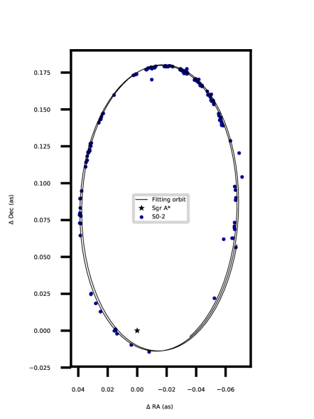
Figure 1: The 145 astrometric positions of the S0-2 star (the blue points) and the fitting orbit (the solid line). Readers should be noticed that this orbit is not the real orbit, which is the projection on the sky plane. The unit as is arcseconds and the origin of coordinates is the position of Sgr A*.

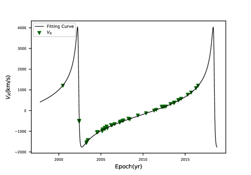
Figure 2: The data of radial velocities of the S0-2 star (the green points) and the fitting curve to describe the change of $V_{R}$ (the solid line).

III.2 Modeling the orbit with relativistic effects

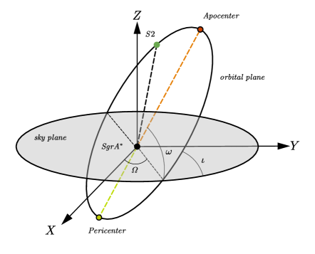
Figure 3: The astrometric positions lie on the sky plane. The Z-axis follows the direction the Solar system points to the Galactic Center and the X-axis points East and the Y-axis points North. $\omega$ is the perihelion argument, $\Omega$ the longitude of ascending node, and $\iota$ the orbital inclination of the processing elliptical orbit for S0-2.

By integrating Eqs. (2.12, 2.13, LABEL:rddot) numerically with given initial conditions for coordinates $\{t(\tau_{0}),r(\tau_{0}),\phi(\tau_{0})\}$ and their derivatives $\{\dot{t}(\tau_{0}),\dot{r}(\lambda_{0}),\dot{\phi}(\lambda_{0})\}$, one can get the theoretical positions of S0-2 star in the self-dual spacetime on the orbital plane. However, the astrometric positions of S0-2 we mentioned in the above subsection is described on the sky plane. The relation between the sky plane and the orbital plane is shown in Fig. 3. Here we would like to mention that, in both planes, the motion of S0-2 star can be well approximated by a precessing elliptical orbit. To compare the theoretical positions and the astrometric positions, we have to make sure all the observational quantities are in the same plane. This can be achieved by projecting the theoretical positions onto the sky plane via

$$X = xB+yG,$$ (3.2)

$$Y = xA+yF,$$ (3.3)

$$Z = xC+yH,$$ (3.4)

where $(X,Y,Z)$ are the coordinates on the sky plane and $(x,y,z)$ are the coordinates on the orbital plane. The coefficients $A,B,C,F,G,H$ can be got from the following formulas

$$A = \cos\Omega\cos\omega-\sin\Omega\sin\omega\cos\iota,$$ (3.5)

$$B = \sin\Omega\cos\omega+\cos\Omega\sin\omega\cos\iota,$$ (3.6)

$$C = \sin\omega\sin\iota,$$ (3.7)

$$F = -\cos\Omega\sin\omega-\sin\Omega\cos\omega\cos\iota,$$ (3.8)

$$G = -\sin\Omega\sin\omega+\cos\Omega\cos\omega\cos\iota,$$ (3.9)

$$H = \cos\omega\sin\iota,$$ (3.10)

where $\omega$ is the perihelion argument, $\Omega$ the longitude of ascending node, and $\iota$ the orbital inclination of the processing elliptical orbit for S0-2. In Fig. 3, we illustrate the relation between the sky and orbital plane and the geometric meanings of $\Omega$, $\omega$, and $\iota$.

Furthermore, considering there are offsets and linear drifts between the gravitational center and the reference frame, we need to introduce $x_{0},y_{0},v_{x0},v_{y0}$ to model it  DoSci

$$X = X(t_{\rm em})+x_{0}+v_{\rm x0}(t_{\rm em})(t_{\rm em}-t_{\rm refer}),$$ (3.11)

$$Y = Y(t_{\rm em})+y_{0}+v_{\rm y0}(t_{\rm em})(t_{\rm em}-t_{\rm refer}),$$ (3.12)

where $t_{\rm refer}$ is the reference epoch for the parameters $x_{0},y_{0},v_{x0},v_{y0}$ and $t_{\rm em}$ is the epoch when the light emit. Here $x_{0},y_{0}$ mean the offsets and $v_{\rm x0}(t_{\rm em})(t_{\rm em}-t_{\rm refer}),v_{\rm y0}(t_{\rm em})(t_{\rm em}-t_{\rm refer})$ mean the linear drifts. For our data, the reference year $t_{\rm refer}=2009.2$ Pinpointing .

We also need to consider several relativistic effects for comparing the theoretical positions with astrometric data.

We first consider the effects of the Romer time delay, which modulates the time of arrival of the light emitted by the star when is farther away or closer to Earth during its orbital motion. The Romer time delay can be expressed as

$$t_{\rm obs}-t_{\rm em}=\frac{Z(t_{\rm em})}{c},$$ (3.13)

where $t_{\rm obs}$ is the epoch when we observe the light and $Z$ can be obtained from Eqs.(3.4). This equation is difficult to solve so one can use an iteration scheme to solve the equation DoSci ; GRAVITY1 :

$$t_{\rm em}^{(i+1)}=t_{\rm obs}-\frac{Z(t_{\rm em}^{(i)})}{c}.$$ (3.14)

For our purpose, after one iteration this equation becomes,

$$t_{\rm em}\approx t_{\rm obs}-\frac{Z(t_{\rm obs})}{c}.$$ (3.15)

Then let us turn to the effects of photon’s frequency shift $\zeta$ which can be related to the radial velocity of the S0-2 star

$$\zeta=\frac{\Delta\nu}{\nu}=\frac{\nu_{\rm em}-\nu_{\rm obs}}{\nu_{\rm obs}}=\frac{V_{\rm R}}{c},$$ (3.16)

where $\nu_{\rm em}$ is the frequency of light when it emits, $\nu_{\rm obs}$ is the frequency when one observes it, and $V_{\rm R}$ is the radial velocity of the S0-2 star. Two relativistic effects can make important contributions to the above frequency shift. One is the Dopple shift $\zeta_{\rm D}$ and the other is the gravitational redshift $\zeta_{G}$.

We first consider the Doppler shift $\zeta_{\rm D}$ which is caused by relative motion between the star and the observer. Due to the high velocity of S0-2, the Doppler shift would cause great impact here

$$\zeta_{\rm D}=\frac{\sqrt{1-\frac{v_{\rm em}^{2}}{c^{2}}}}{1-\bm{n}\cdot\bm{v}_{\rm em}},$$ (3.17)

where $v_{em}$ is the velocity at $t_{em}$, $\bm{n}\cdot\bm{v}_{\rm em}$ is the velocity projected on to the sight of the light, which is known as the radial velocity. The gravitational shift $\zeta_{\rm G}$ is a GR effect and this frequency shift would become significant under strong gravitational fields which reads

$$\zeta_{\rm G}=\frac{1}{\sqrt{-g_{00}}}.$$ (3.18)

Therefore, we get

$$\zeta=\zeta_{\rm D}\cdot\zeta_{\rm G}-1.$$ (3.19)

Also, considering that the Sgr A* might moving toward the sun, which would affect the velocity, we introduce $v_{\rm z0}$ here to model the $V_{\rm R}$ Reid:2006cu .

$$V_{\rm R}=c\cdot\zeta+v_{\rm z0}.$$ (3.20)

III.3 Analysis of Monte Carlo Markov Chain

In this paper, we carry out the analysis of the MCMC implemented by emcee emcee to obtain the constraints on the self-dual spacetime. We explore the following parameters

$$\{M,R_{0},a,e,\iota,\omega,\Omega,t_{\rm apo},x_{0},y_{0},v_{x_{0}},v_{y_{0}},v_{z_{0}},P\},$$

to fit the theoretical orbits to the publicly available data as described in Sec.III.A. Here $M$ and $R_{0}$ are the mass of the central black hole and the distance between the Earth and the black hole, $\{a,e,\iota,\omega,\Omega,t_{\rm apo}\}$ are the six orbital elements which describe the osculating elliptical orbit of the S0-2 star. The five parameters $\{x_{0},y_{0},v_{x_{0}},v_{y_{0}},v_{z_{0}}\}$ represent the zero-point offsets and drifts of the reference frame with respect to the mass centroid, and $P$ is the polymeric function arsing from the self-dual spacetime in LQG. Here we would like to note that the orbit of S0-2 is not an exact ellipse, but a processing ellipse. For every single point of the orbit one can associate a corresponding ellipse which is called the osculating ellipse and described by the above orbital elements.

To carry out our MCMC analysis with the above parameter space, we use two prior sets, the Gaussian and uniform priors respectively, for the 13 orbital parameters. The Gaussian priors are set to be centered on the best values given in GRAVITY2 . For the polymeric function $P$ in the self-dual spacetime, we use uniform prior for both simulations. The prior sets used for our MCMC analysis is summarized in Table. 1. Similar prior sets have also been used in constraining different modified theories of gravity with astrometric data of S0-2 Borka:2021omc ; deMartino:2021daj ; DellaMonica:2021xcf ; DellaMonica:2021fdr ; DAddio:2021smm .

Table 1: Two different prior sets used for our MCMC analysis. The Gaussian priors are set to be centered on the best values given in GRAVITY2 . In this table, the units $M_{\rm\odot}$ is the solar mass, kpc is the kiloparsec, mas is the milliarcsecond, ^∘ is the degree, and yr is the year.

	Gaussian prior		Uniform prior
Paramaters	$\mu$	$\sigma$	-
$M\;(10^{6}M_{\rm\odot})$	4.261	0.012	[0, 10]
$R_{0}$ (kpc)	8.2467	0.0093	[5, 10]
$a$ (mas)	125.058	0.04	[120, 130]
$e$	0.884649	0.00008	[0.5, 1.5]
$\iota$ (∘)	134.567	0.033	[130, 140]
$\omega$ (∘)	66.263	0.031	[60, 70]
$\Omega$ (∘)	228.171	0.031	[220, 240]
$t_{\rm apo}$ (yr)	2010.38	0.00016	[2009, 2011]
$x_{0}$ (mas)	-0.90	0.14	[-50, 50]
$y_{0}$ (mas)	0.07	0.12	[-50, 50]
$v_{\rm x_{0}}$ (mas/yr)	0.080	0.010	[-50, 50]
$v_{\rm y_{0}}$ (mas/yr)	0.0341	0.00096	[-50, 50]
$v_{\rm z_{0}}$ (km/s)	-1.6	1.4	[-50, 50]
$P$	-	-	[0, 1]

As we mentioned in Sec.III.A, three different parts of data are employed in our MCMC analysis. For this reason, the likelihood function $\mathcal{L}$ consists of three parts, i.e.

$$\log{\cal L}=\log{\cal L}_{\rm AP}+\log{\cal L}_{\rm VR}+\log{\cal L}_{\rm pro},$$ (3.22)

where $\log{\cal L}_{\rm AP}$ denotes the likelihood of the 145 astrometric positional data

$$\log{\cal L}_{\rm AP} = -\frac{1}{2}\sum_{i}\frac{(X_{\rm obs}^{i}-X_{\rm the}^{i})^{2}}{(\sigma^{i}_{X,{\rm obs}})^{2}}$$ (3.23)

$$-\frac{1}{2}\sum_{i}\frac{(Y_{\rm obs}^{i}-Y_{\rm the}^{i})^{2}}{(\sigma^{i}_{Y,{\rm obs}})^{2}},$$

$\log{L}_{\rm VR}$ represents the likelihood of the 45 data of the radial velocities

$$\log{L}_{\rm VR}-\frac{1}{2}\sum_{i}\frac{(V_{\rm R,obs}^{i}-V_{\rm R,the}^{i})^{2}}{(\sigma^{i}_{V_{\rm R,obs}})^{2}},$$ (3.24)

and $\log{\cal L}_{\rm pro}$ is the likelihood of the orbital precession

$$\log{\cal L}_{\rm pro}=-\frac{1}{2}\frac{(\Delta\phi_{\rm obs}-\Delta\phi_{\rm the})^{2}}{\sigma^{2}_{\Delta\phi,{\rm obs}}}.$$ (3.25)

Here $X_{\rm obs}^{i}$, $Y_{\rm obs}^{i}$, and $V_{\rm R,obs}^{i}$ are the data of the astrometric positions and radial velocities, and $X_{\rm the}^{i}$, $Y_{\rm the}^{i}$, and $V_{\rm R,the}^{i}$ are the corresponding theoretical predictions. $\Delta\phi_{\rm obs}$ represents the measurements of the orbital precession given in (3.1) and $\Delta\phi_{\rm the}$ is given by (2.15) with given values of $P$. In the above expressions, $\sigma^{i}_{x,{\rm obs}^{i}}$ denote the corresponding statistical uncertainty for the associated quantities.

III.4 Results and Discussions

With the setup described in the above subsections, we explore the above mentioned 14-dimensional parameter space through an analysis of MCMC. In Fig. 4 and Fig. 6, we illustrate the full posterior distributions of our 14-dimensional parameter space of our orbital model for two sets of priors respectively. On the contour plots of this figure, the shaded regions show the 68%, 90%, and 95% confidence levels (C.L.) of the posterior probability density distributions of the entire set of parameters, respectively. The corresponding best fit values of these 14 parameters for two sets of priors are presented in Table. 2. The comparison of the orbit of these best-fit values and the astrometric data is also presented in Fig. 1. The results are presented in Fig. 4 , Fig. 6 and Table. 2 .

Table 2: The best-fit values of the parameters of the orbital model of S0-2 in the self-dual spacetime, resulting from the MCMC analysis. The upper bound on $P$ is derived from the posterior region at 95% C.L..

Parameters	Best-fit values
	Gaussian	uniform
$M\;(10^{6}M_{\odot})$	4.38	4.46
$R_{0}$ (kpc)	8.17	8.02
$a$ (mas)	125.06	127.98
$e$	0.8844	0.8872
$\iota$ (∘)	134.61	133.72
$\omega$ (∘)	66.03	65.84
$\Omega$ (∘)	228.102	226.97
$t_{\rm apo}$ (yr)	2010.34	2010.38
$x_{0}$ (mas)	-0.35	1.06
$y_{0}$ (mas)	0.0005	-2.51
$v_{\rm x_{0}}$ (mas/yr)	0.084	0.134
$v_{\rm y_{0}}$ (mas/yr)	0.041	0.020
$v_{\rm z_{0}}$ (km/s)	-0.96	13.42
$P$	$<$ 0.043	$<$ 0.056

In order to estimate the observational constraint on the polymeric function $P$ of LQG, we plot the marginalized posterior distribution of $P$ in Fig. 5 and Fig  7. Then the upper bounds on $P$ can be calculated from the corresponding posterior distribution of $P$. We find the polymeric function $P$ can be constrained at 95% confidence level to be

$$P<0.043,$$ (3.26)

for Gaussian prior and

$$P<0.056,$$ (3.27)

for uniform prior respectively.

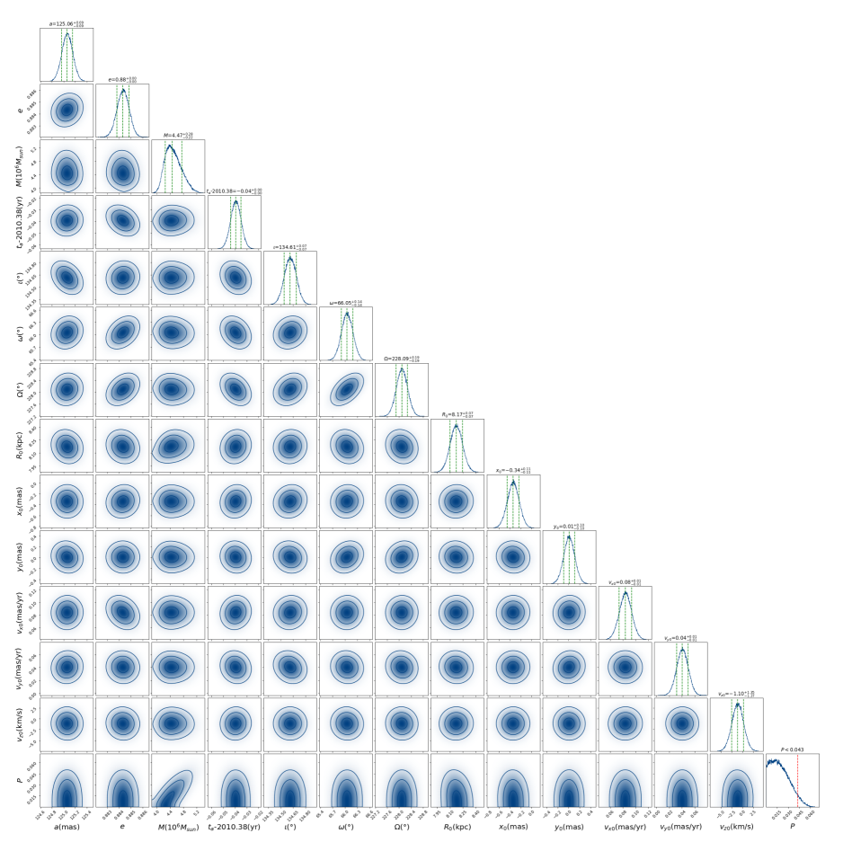
Figure 4: The posterior distribution of the orbital parameters of the S0-2 star and the polymeric function $P$ of the self-dual spacetime with Gaussian priors for the orbital parameters.

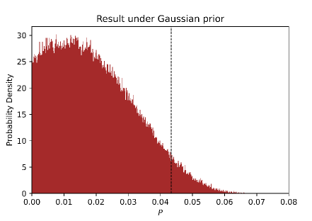
Figure 5: This figure is picked from Fig. 4 to show more details. The upper limit of $P$ is 0.043 at 95% confidence level.

The constraints we obtain here are both a little bit stronger (but compatible) than the bound $P<0.067$ obtained in Zhu:2020tcf by directly using the error of the measurement of the orbital precession of the S0-2 star. However, it is much weaker than those obtained from the measurement of the gravitational time delay by the Cassini mission, the deflection angle of light by the Sun, and the perihelion advance of Mercury Zhu:2020tcf . Although the observational constraints from the S0-2 is not accurate enough with respect to other type observations, our results show that the observational data from the observations of S0-2 star at the galactic center does have the capacity for constraining black hole parameters beyond those in GR. In addition, we would like to mention that those tighter constraints mentioned above are all derived from the observations at the scale of the solar system, our results represent a bound on $P$ from a very different environment of strong gravity regime.

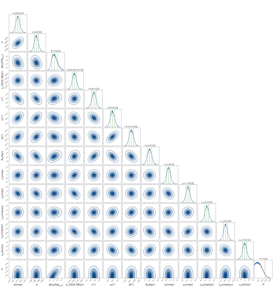
Figure 6: The posterior distribution of the orbital parameters of the S0-2 star and the polymeric function $P$ of the self-dual spacetime with uniform priors for the orbital parameters.

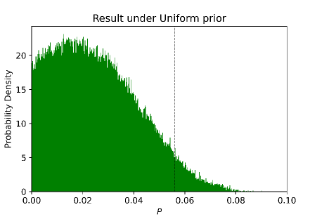
Figure 7: This figure is picked from Fig. 6 to show more details. The upper limit of $P$ is 0.056 at 95% confidence level.

IV Conclusions

In this paper, we consider the effects of the self-dual spacetime of LQG on the orbit of the S0-2 star orbiting Sgr A* in the central region of our Milky Way. The effects of LQG may not only lead to signatures on the orbits of the S0-2 star, but also affect its overall peri- centre advance. We also compare the effects of the self-dual spacetime with the publicly available astrometric and spectroscopic data, including the astrometric positions, the radial velocities, and the orbital precession for the S0-2 star. With these data, we perform a MCMC simulation to probe the possible LQG effects on the orbit of the S0-2 star. We do not find any significant evidence of the self-dual space-time and thus place an upper bound at 95% confidence level on the polymeric function $P<0.043$ and $P<0.056$, corresponding to the Gaussian and uniform priors for orbital parameters, respectively. This bounds lead to a constraints on the polymeric parameter $\delta$ of LQG to be $|\delta|<1.82$ and $|\delta|<2.11$ respectively. Finally, we would like to mention that we only consider the static self-dual spacetime in this paper and ignore the effects of the angular momentum of the spacetime. For all the observational effects we considered in this paper, the effects due to rotation of the central black hole are expected to be very small.

References

- (1) R. J. Adler, Six easy roads to the Planck scale, Am. J. Phys. 78, 925 (2010).
- (2) Y. J. Ng, Selected topics in Planck scale physics, Mod. Phys. Lett. A 18, 1073 (2003).
- (3) A. Borde and A. Vilenkin, Eternal inflation and the initial singularity, Phys. Rev. Lett. 72, 3305 (1994).
- (4) A. Borde, A. H. Guth, and A. Vilenkin, Inflationary Space-times are Incomplete in Past Directions, Phys. Rev. Lett. 90, 151301 (2003).
- (5) S. W. Hawking, G. F. R. Ellis, The Large Scale Structure of Space-Time, 21. print., [repr.] Cambridge Univ. Press, Cambridge, (2008).
- (6) A. Ashtekar and P. Singh, Loop quantum cosmology: a status report, Class. Quantum Grav. 28, 213001 (2011).
- (7) A. Ashtekar and A. Barrau, Loop quantum cosmology: from pre-inflationary dynamics to observations, Class. Quantum Grav. 32, 234001 (2015).
- (8) A. Ashtekar and M. Bojowald, Quantum geometry and the Schwarzschild singularity, Class. Quant. Grav. 23, 391-411 (2006) [arXiv:gr-qc/0509075 [gr-qc]].
- (9) L. Modesto, Semiclassical Loop Quantum Black Hole, Int. J. Theor. Phys. 49, 1649 (2010).
- (10) L. Modesto and I. Premont-Schwarz, Self-dual black holes in loop quantum gravity: Theory and phenomenology, Phys. Rev. D 80, 064041 (2009).
- (11) S. Sahu, K. Lochan and D. Narasimha, Gravitational lensing by self-dual black holes in loop quantum gravity, Phys. Rev. D 91, 063001 (2015).
- (12) A. Ashtekar, J. Olmedo, and P. Singh, Quantum Transfiguration of Kruskal Black Holes, Phys. Rev. Lett. 121, 241301 (2018).
- (13) A. Ashtekar, J. Olmedo, and P. Singh, Quantum extension of the Kruskal spacetime, Phys. Rev. D 98, 126003 (2018).
- (14) M. Bojowald, S. Brahma, and D. -h. Yeom, Effective line elements and black-hole models in canonical loop quantum gravity, Phys. Rev. D 98, 046015 (2018).
- (15) E. Alescia, S. Bahrami, D. Pranzetti, Quantum gravity predictions for black hole interior geometry, Phys. Lett. B 797, 134908 (2019).
- (16) M. Assanioussi, A. Dapor, and K. Liegener, Perspectives on the dynamics in a loop quantum gravity effective description of black hole interiors, Phys. Rev. D 101, 026002 (2020).
- (17) R. Gambini, J. Olmedo and J. Pullin, Loop Quantum Black Hole Extensions Within the Improved Dynamics, Front. Astron. Space Sci. 8, 74 (2021).
- (18) A. García-Quismondo and G. A. M. Marugán, Exploring Alternatives to the Hamiltonian Calculation of the Ashtekar-Olmedo-Singh Black Hole Solution, Front. Astron. Space Sci. 0, 115 (2021).
- (19) A. Perez, Black holes in loop quantum gravity, Rep. Prog. Phys. 80, 126901 (2017).
- (20) A. Barrau, K. Martineau and F. Moulin, A Status Report on the Phenomenology of Black Holes in Loop Quantum Gravity: Evaporation, Tunneling to White Holes, Dark Matter and Gravitational Waves, Universe 4, 102 (2018).
- (21) C. Rovelli, Black Hole Evolution Traced Out with Loop Quantum Gravity, APS Physics 11, 127 (2018).
- (22) A. Ashtekar, Black hole evaporation: A perspective from loop quantum gravity, Universe 2, 6 (2021).
- (23) W. C. Gan, N. O. Santos, F. W. Shu and A. Wang, Towards understanding of loop quantum black holes, Phys. Rev. D 102, 124030 (2020).
- (24) E. Alesci and L. Modesto, Particle Creation by Loop Black Holes, Gen. Rel. Grav. 46, 1656 (2014).
- (25) J. H. Chen and Y. J. Wang, Complex frequencies of a massless scalar field in loop quantum black hole spacetime, Chin. Phys. B 20, 030401 (2011).
- (26) A. Dasgupta, Entropy Production and Semiclassical Gravity, SIGMA 9, 013 (2013). .
- (27) A. Barrau, C. Rovelli and F. Vidotto, Fast Radio Bursts and White Hole Signals, Phys. Rev. D 90, 127503 (2014).
- (28) S. Hossenfelder, L. Modesto and I. Premont-Schwarz, Emission spectra of self-dual black holes, arXiv:1202.0412 [gr-qc].
- (29) M. B. Cruz, C. A. S. Silva and F. A. Brito, Gravitational axial perturbations and quasinormal modes of loop quantum black holes, Eur. Phys. J. C 79, 157 (2019).
- (30) F. Moulin, K. Martineau, J. Grain, and A. Barrau, Quantum Fields in the Background Spacetime of a Polymeric Loop Black Hole, Class. Quant. Grav. 36, 125003 (2019).
- (31) F. Moulin, A. Barrau and K. Martineau, An overview of quasinormal modes in modified and extended gravity, Universe 5, 202 (2019).
- (32) M. B. Cruz, F. A. Brito and C. A. S. Silva, Polar gravitational perturbations and quasinormal modes of a loop quantum gravity black hole, Phys. Rev. D 102, 044063 (2020).
- (33) J. S. Santos, M. B. Cruz and F. A. Brito, Quasinormal modes of a massive scalar field nonminimally coupled to gravity in the spacetime of self-dual black hole, Eur. Phys. J. C 81, 1082 (2021).
- (34) C. Liu, T. Zhu, Q. Wu, K. Jusufi, M. Jamil, M. Azreg-Aïnou and A. Wang, Shadow and Quasinormal Modes of a Rotating Loop Quantum Black Hole, Phys. Rev. D 101, 084001 (2020).
- (35) T. Zhu and A. Wang, Observational tests of the self-dual spacetime in loop quantum gravity, Phys. Rev. D 102, 124042 (2020).
- (36) S. B. Giddings, Searching for quantum black hole structure with the Event Horizon Telescope, Universe 5, 201 (2019).
- (37) S. B. Giddings, Astronomical tests for quantum black hole structure, Nature Astron. 1, 0067 (2017).
- (38) S. B. Giddings and D. Psaltis, Event Horizon Telescope Observations as Probes for Quantum Structure of Astrophysical Black Holes, Phys. Rev. D 97, 084035 (2018).
- (39) H. M. Haggard and C. Rovelli, Quantum Gravity Effects around Sagittarius A*, Int. J. Mod. Phys. D 25, 1644021 (2016).
- (40) A. Barrau, K. Martineau, J. Martinon and F. Moulin, Quasinormal modes of black holes in a toy-model for cumulative quantum gravity, Phys. Lett. B 795, 346-350 (2019).
- (41) Y. C. Liu, J. X. Feng, F. W. Shu and A. Wang, Extended geometry of Gambini-Olmedo-Pullin polymer black hole and its quasinormal spectrum, Phys. Rev. D 104, 106001 (2021).
- (42) R. G. Daghigh, M. D. Green and G. Kunstatter, Scalar Perturbations and Stability of a Loop Quantum Corrected Kruskal Black Hole, Phys. Rev. D 103, 084031 (2021).
- (43) M. Bouhmadi-López, S. Brahma, C.-Y. Chen, P. Chen, and D. Yeom, A consistent model of non-singular Schwarzschild black hole in loop quantum gravity and its quasinormal modes, J. Cosmol. Astropart. Phys. 2020, 066 (2020).
- (44) Q. M. Fu and X. Zhang, Gravitational lensing by a black hole in effective loop quantum gravity, arXiv:2111.07223 [gr-qc].
- (45) S. Brahma, C. Y. Chen and D. h. Yeom, Testing Loop Quantum Gravity from Observational Consequences of Nonsingular Rotating Black Holes, Phys. Rev. Lett. 126, 181301 (2021).
- (46) D. del-Corral and J. Olmedo, Isospectrality of quasinormal modes in nonrotating loop quantum gravity black holes, arXiv:2201.09584 [gr-qc].
- (47) A. M. Ghez, S. Salim, N. N. Weinberg, J. R. Lu, T. Do, J. K. Dunn, K. Matthews, M. R. Morris, S. Yelda, E. E. Becklin, T. Kremenek, M. Milosavljevic, and J. Naiman, Measuring Distance and Properties of the Milky Way’s Central Supermassive Black Hole with Stellar Orbits, Astrophys. J. 689, 1044 (2008).
- (48) R. Genzel, F. Eisenhauer, and S. Gillessen, The Galactic Center Massive Black Hole and Nuclear Star Cluster, Rev. Mod. Phys. 82, 3121 (2010).
- (49) T. Johannsen, Sgr A* and General Relativity, Class. Quant. Grav. 33, 113001 (2016).
- (50) R. Abuter et al. [GRAVITY], Detection of the gravitational redshift in the orbit of the star S2 near the Galactic centre massive black hole, Astron. Astrophys. 615, L15 (2018) .
- (51) R. Abuter et al. [GRAVITY], A Geometric Distance Measurement to the Galactic Center Black Hole with 0.3% Uncertainty, Astron. Astrophys. 625, L10 (2019).
- (52) T. Do, A. Hees, A. Ghez, G. D. Martinez, D. S. Chu, S. Jia, S. Sakai, J. R. Lu, A. K. Gautam and K. K. O’Neil, et al., Relativistic redshift of the star S0-2 orbiting the Galactic center supermassive black hole, Science 365, 664 (2019).
- (53) R. Abuter et al. [GRAVITY], Detection of the Schwarzschild precession in the orbit of the star S2 near the Galactic centre massive black hole, Astron. Astrophys. 636, L5 (2020).
- (54) D. Psaltis, N. Wex and M. Kramer, A Quantitative Test of the No-Hair Theorem with Sgr A* using stars, pulsars, and the Event Horizon Telescope, Astrophys. J. 818, 121 (2016).
- (55) H. Qi, R. O. Shaughnessy, and P. Brady, Testing the black hole no-hair theorem with Galactic Center stellar orbits, Phys. Rev. D 103, 084006 (2021).
- (56) D. Benisty and A. C. Davis, Dark energy interactions near the Galactic Center, Phys. Rev. D 105, 024052 (2022).
- (57) L. Hui, D. Kabat, X. Li, L. Santoni and S. S. C. Wong, Black Hole Hair from Scalar Dark Matter, J. Cosmol. Astropart. Phys 06, 038 (2019).
- (58) G. Heißel, T. Paumard, G. Perrin and F. Vincent, The dark mass signature in the orbit of S2, arXiv:2112.07778 [astro-ph.GA].
- (59) S. Nampalliwar, S. K., K. Jusufi, Q. Wu, M. Jamil and P. Salucci, Modelling the Sgr A* Black Hole Immersed in a Dark Matter Spike, Astrophys. J. 916 116 (2021).
- (60) A. F. Zakharov, Testing the Galactic Centre potential with S-stars, arXiv:2108.09709 [astro-ph.GA].
- (61) E. A. Becerra-Vergara, C. R. Argüelles, A. Krut, J. A. Rueda and R. Ruffini, Hinting a dark matter nature of Sgr A* via the S-stars, Mon. Not. Roy. Astron. Soc. 505, L64-L68 (2021).
- (62) A. Hees, T. Do, A. M. Ghez, G. D. Martinez, S. Naoz, E. E. Becklin, A. Boehle, S. Chappell, D. Chu and A. Dehghanfar, et al., Testing General Relativity with stellar orbits around the supermassive black hole in our Galactic center, Phys. Rev. Lett. 118, 211101 (2017).
- (63) Y. Fang and X. Chen, Stellar rotation as a new observable to test general relativity in the Galactic Center, Phys. Rev. D 103, 063041 (2021).
- (64) D. Borka, V. B. Jovanović, S. Capozziello, A. F. Zakharov and P. Jovanović, Estimating the Parameters of Extended Gravity Theories with the Schwarzschild Precession of S2 Star, Universe 7, 407 (2021).
- (65) I. de Martino, R. della Monica and M. de Laurentis, f(R) gravity after the detection of the orbital precession of the S2 star around the Galactic Center massive black hole, Phys. Rev. D 104, L101502 (2021).
- (66) R. Della Monica, I. de Martino and M. de Laurentis, Orbital precession of the S2 star in Scalar–Tensor–Vector Gravity, Mon. Not. Roy. Astron. Soc. 510, 4757-4766 (2022).
- (67) R. Della Monica and I. de Martino, Unveiling the Nature of SgrA* with the Geodesic Motion of S-Stars, J. Cosmol. Astropart. Phys. 2022, 007 (2022).
- (68) A. D’Addio, S-star dynamics through a Yukawa–like gravitational potential, Phys. Dark Univ. 33, 100871 (2021).
- (69) A. Ashtekar, Black hole evaporation: A perspective from loop quantum gravity, Universe 6, 21 (2020).
- (70) L. Modesto, Loop quantum black hole, Class. Quant. Grav. 23, 5587-5602 (2006) [arXiv:gr-qc/0509078 [gr-qc]].
- (71) M. Campiglia, R. Gambini and J. Pullin, Loop quantization of spherically symmetric midi-superspaces : The Interior problem, AIP Conf. Proc. 977, no.1, 52-63 (2008) [arXiv:0712.0817 [gr-qc]].
- (72) J. B. Achour, J. Grain, and K. Noui, Loop Quantum Cosmology with Complex Ashtekar Variables, Class. Quantum Grav. 32, 025011 (2015).
- (73) E. Frodden, M. Geiller, K. Noui and A. Perez, Black Hole Entropy from complex Ashtekar variables, EPL 107, 10005 (2014).
- (74) J. Ben Achour, A. Mouchet and K. Noui, Analytic Continuation of Black Hole Entropy in Loop Quantum Gravity, JHEP 06, 145 (2015).
- (75) M. Han, Black Hole Entropy in Loop Quantum Gravity, Analytic Continuation, and Dual Holography, arXiv:1402.2084 [gr-qc].
- (76) S. Carlip, A Note on Black Hole Entropy in Loop Quantum Gravity, Class. Quant. Grav. 32, 155009 (2015).
- (77) V. Taveras and N. Yunes, The Barbero-Immirzi Parameter as a Scalar Field: K-Inflation from Loop Quantum Gravity?, Phys. Rev. D 78, 064070 (2008).
- (78) K. A. Meissner, Black hole entropy in Loop Quantum Gravity, Class. Quantum Grav. 21, 5245 (2004).
- (79) S. Gillessen, P. M. Plewa, F. Eisenhauer, R. Sari, I. Waisberg, M. Habibi, O. Pfuhl, E. George, J. Dexter, S. von Fellenberg, T. Ott, and R. Genzel, An Update on Monitoring Stellar Orbits in the Galactic Center, Astrophys. J. 837 30 (2017).
- (80) P. M. Plewa et al., Pinpointing the Near-Infrared Location of Sgr A* by Correcting Optical Distortion in the NACO Imager, Mon. Not. R. Astron. Soc. 453, 3235 (2015).
- (81) M. J. Reid, K. M. Menten, S. Trippe, T. Ott and R. Genzel, The Position of Sagittarius A*. 3. Motion of the Stellar Cusp, Astrophys. J. 659, 378-388 (2007).
- (82) D. Foreman-Mackey, D. W. Hogg, D. Lang, & J. Goodman, emcee: The MCMC Hammer, PASP 125 306 (2013).