Farthest-point Voronoi diagrams in the presence of rectangular obstacles

Abstract

We present an algorithm to compute the geodesic $L_{1}$ farthest-point Voronoi diagram of $m$ point sites in the presence of $n$ rectangular obstacles in the plane. It takes $O(nm+n\log n+m\log m)$ construction time using $O(nm)$ space. This is the first optimal algorithm for constructing the farthest-point Voronoi diagram in the presence of obstacles. We can construct a data structure in the same construction time and space that answers a farthest-neighbor query in $O(\log(n+m))$ time.

1 Introduction

A Voronoi diagram of a set of sites is a subdivision of the space under consideration into subspaces by assigning points to sites with respect to a certain proximity. Typical Voronoi assignment models are the nearest-point model and the farthest-point model where every point is assigned to its nearest site and its farthest site, respectively. There are results for computing Voronoi diagrams in the plane [1, 13, 14, 25], under different metrics [9, 17, 18, 24], or for various types of sites [2, 8, 23].

For $m$ point sites in the plane, the nearest-point and farthest-point Voronoi diagrams of the sites can be constructed in $O(m\log m)$ time [14, 25]. When the sites are contained in a simple polygon with no holes, the distance between any two points in the polygon, called the geodesic distance, is measured as the length of the shortest path contained in the polygon and connecting the points (called the geodesic path). There has been a fair amount of work computing the geodesic nearest-point and farthest-point Voronoi diagrams of $m$ point sites in a simple $n$-gon [3, 4, 21, 22] to achieve the lower bound $\Omega(n+m\log m)$ [3]. Recently, optimal algorithms of $O(n+m\log m)$ time were given for the geodesic nearest-point Voronoi diagram [20] and for the geodesic farthest-point Voronoi diagram [26].

The problem of computing Voronoi diagrams is more challenging in the presence of obstacles. Each obstacle plays as a hole and there can be two or more geodesic paths connecting two points avoiding those holes. The geodesic nearest-point Voronoi diagram of $m$ point sites can be computed in $O(m\log m+k\log k)$ time by applying the continuous Dijkstra paradigm [16], where $k$ is the number of total vertices of obstacles. However, no optimal algorithm is known for the farthest-point Voronoi diagram in the presence of obstacles in the plane, even when the obstacles are of elementary shapes such as axis-aligned line segments and rectangles. The best result of the geodesic farthest-point Voronoi diagram known so far takes $O(mk\log^{2}(m+k)\log k)$ time by Bae and Chwa [5]. They also showed that the total complexity of the geodesic farthest-point Voronoi diagram is $\Theta(mk)$.

In the presence of $n$ rectangular obstacles under $L_{1}$ metric, there are some work for farthest-neighbor queries. Ben-Moshe et al. [7] presented a data structure with $O(nm\log(n+m))$ construction time and $O(nm)$ space for $m$ point sites that supports farthest point queries in $O(\log(n+m))$ time. They also showed that the $L_{1}$ geodesic farthest-point Voronoi diagram has complexity $\Theta(nm)$, but without presenting any algorithm for computing the diagram. Later Ben-Moshe et al. [6] gave a tradeoff between the query time and the preprocessing/space such that a data structure of size $O((n+m)^{1.5})$ can be constructed in $O((n+m)^{1.5}\log^{2}(n+m))$ to support farthest point queries in $O((n+m)^{0.5}\log(n+m))$ time.

The geodesic center of a set of objects in a polygonal domain is the set of points in the domain that minimize the maximum geodesic distance from input objects. Thus, it can be obtained once the geodesic farthest-point Voronoi diagram of the objects is constructed. For $m$ points in the presence of $n$ axis-aligned rectangular obstacles in the plane, Choi et al. [10] showed that the geodesic center of the points under the $L_{1}$ metric consists of $\Theta(nm)$ connected regions and they gave an $O(n^{2}m)$-time algorithm to compute the geodesic center. Later, Ben-Moshe et al. [7] gave an $O(nm\log(n+m))$-time algorithm for the problem.

Our Result.

In this paper, we present an algorithm that computes the geodesic $L_{1}$ farthest-point Voronoi diagram of $m$ points in the presence of $n$ rectangular obstacles in the plane in $O(nm+n\log n+m\log m)$ time using $O(nm)$ space. The running time and space complexity of our algorithm match the time and space bounds of the Voronoi diagram. Thus, it is the first optimal algorithm for computing the geodesic farthest-point Voronoi diagram in the presence of obstacles.

To do this, we construct a data structure for $L_{1}$ farthest-neighbor queries in $O(nm+n\log n+m\log m)$ time using $O(nm)$ space. This improves upon the results by Ben-Moshe et al. [7], and the construction time and space are the best among the data structures supporting $O(\log(n+m))$ query time for $L_{1}$ farthest neighbors. Then we present an optimal algorithm to compute the explicit geodesic $L_{1}$ farthest-point Voronoi diagram in $O(nm+n\log n+m\log m)$ time using $O(nm)$ space, which matches the time and space lower bounds of the diagram.

As a byproduct, we compute the geodesic center under the $L_{1}$ metric in $O(nm+n\log n+m\log m)$ time. This result improves upon the algorithm by Ben-Moshe et al. [7].

Outline.

First, we construct four farthest-point maps, one for each of the four axis directions, either the $x$- or $y$-axis, and either positive or negative. In the course, we construct a data structure for $L_{1}$ farthest-neighbor queries in $O(nm+n\log n+m\log m)$ time using $O(nm)$ space. For each axis direction, we apply the plane sweep technique with a line orthogonal to the direction and moving along the direction. During the sweep, we maintain the status of the sweep line in a balanced binary search tree and its associated structures while handling events induced by the point sites and the sides of rectangles parallel to the sweep line. There are $m$ events induced by point sites and $O(n)$ events induced by rectangles. After sorting the events in $O(n\log n+m\log m)$ time, we show that we can handle all events induced by point sites in $O(nm)$ time. Additionally, we show that each event induced by a rectangle can be handled in $O(m+\log n)$ time. By the plane sweep, we construct a data structure consisting of $O(n+m)$ line segments parallel to the sweep line and $O(nm)$ points in $O(nm+n\log n+m\log m)$ time in total. Given a query, it uses axis-aligned ray shooting queries on the data structure to find the farthest site from the query. The four farthest-point maps are planar subdivisions, and they can be constructed during the plane sweep in the same time and space.

With the four farthest-point maps and the data structure for farthest-neighbor queries, we construct the geodesic $L_{1}$ farthest-point Voronoi diagram explicitly. First, we decompose the plane, excluding the holes, into rectangular faces using vertical line segments, each extended from a vertical side of a hole. Then, we partition each face in the decomposition into zones such that the farthest-point Voronoi diagram restricted to a zone coincides with the corresponding region of a farthest-point map. This partition is done by using the boundary between two farthest-point maps, which can be computed by traversing the cells in the two maps in which the boundary lies. Finally, we glue the corresponding regions along the boundaries of zones, and then glue all adjacent faces along their boundaries to obtain the geodesic $L_{1}$ farthest-point Voronoi diagram. We show that this can be done in $O(nm+n\log n+m\log m)$ time in total.

For the centers of $m$ points in the presence of $n$ axis-aligned rectangles in the plane, we can find them from the farthest-point Voronoi diagram in time linear to the complexity of the diagram.

2 Preliminaries

Let $\mathsf{R}$ be a set of $n$ open disjoint rectangles and $\mathsf{S}$ be a set of $m$ point sites lying in the free space $\mathsf{F}=\mathbb{R}^{2}-\bigcup_{R\in\mathsf{R}}R$. We consider the $L_{1}$ metric. For ease of description, we omit $L_{1}$. We use $x(p)$ and $y(p)$ to denote the $x$-coordinate and $y$-coordinate of a point $p$, respectively. For two points $p$ and $q$ in $\mathsf{F}$, we use $pq$ to denote the line segment connecting them. Whenever we say a path connecting two points in $\mathsf{F}$, it is a path contained in $\mathsf{F}$. There can be more than one geodesic path connecting two points $p$ and $q$ avoiding the holes. We use $\pi(p,q)$ to denote a fixed geodesic path connecting $p$ and $q$, and use $d(p,q)$ to denote the geodesic distance between $p$ and $q$, which is the length of $\pi(p,q)$.

We make a general position assumption that no point in $\mathsf{F}$ is equidistant from four or more distinct sites. We use $f(p)$ to denote the set of sites of $\mathsf{S}$ that are farthest from a point $p\in\mathsf{F}$ under the geodesic distance, that is, a site $s$ is in $f(p)$ if and only if $d(s,p)\geq d(s^{\prime},p)$ for all $s^{\prime}\in\mathsf{S}$. If there is only one farthest site, we use $f(p)$ to denote the site.

A horizontal line segment $\ell$ can be represented by the two $x$-coordinates $x_{1}(\ell)$ and $x_{2}(\ell)$ of its endpoints ($x_{1}(\ell)<x_{2}(\ell)$) and the $y$-coordinate $y(\ell)$ of them. For an axis-aligned rectangle $R$, let $x_{1}(R)$ and $x_{2}(R)$ denote the $x$-coordinates of the left and right sides of $R$.

A path is $x$-monotone if and only if the intersection of the path with any line perpendicular to the $x$-axis is connected. Likewise, a path is $y$-monotone if and only if the intersection of the path with any line perpendicular to the $y$-axis is connected. A path is $xy$-monotone if and only if the path is $x$-monotone and $y$-monotone. Observe that if a path connecting two points is $xy$-monotone, it is a geodesic path connecting the points.

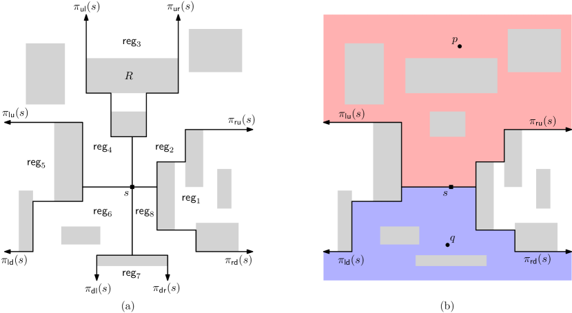
Figure 1: Gray rectangles are holes. (a) The eight paths partition $\mathsf{F}$ into eight regions $\textsf{reg}_{1},\ldots,\textsf{reg}_{8}$. Region $\textsf{reg}_{3}$ consists of two regions separated by a rectangle $R$. (b) Every geodesic path from $s$ to $p$ is ${y^{+}}$-monotone and $p$ is ${y^{+}}$-reachable from $s$. Every geodesic path from $s$ to $q$ is ${y^{-}}$-monotone and $q$ is ${y^{-}}$-reachable from $s$.

2.1 Eight Monotone Paths from a Point

Choi and Yap [11] gave a way of partitioning the plane with rectangular holes into eight regions using eight $xy$-monotone paths from a point. We use their method to partition $\mathsf{F}$ as follows. Consider a horizontal ray emanating from a point $s=p_{1}\in\mathsf{F}$ going rightwards. The ray stops when it hits a rectangle $R\in\mathsf{R}$ at a point $p_{1}^{\prime}$. Let $p_{2}$ be the top-left corner of $R$. We repeat this process by taking a horizontal ray from $p_{2}$ going rightwards until it hits a rectangle, and so on. Then we obtain an $xy$-monotone path $\pi_{\mathsf{ru}}(s)=p_{1}p_{1}^{\prime}p_{2}p_{2}^{\prime}\ldots$ from $s$ that alternates going rightwards and going upwards.

By choosing two directions, one going either rightwards or leftwards horizontally, and one going either upwards or downwards vertically, and ordering the chosen directions, we define eight rectilinear $xy$-monotone paths with directions: rightwards-upwards (ru), upwards-rightwards (ur), upwards-leftwards (ul), leftwards-upwards (lu), leftwards-downwards (ld), downwards-leftwards (dl), downwards-rightwards (dr), and rightwards-downwards (rd). Let $\pi_{\delta}(s)$ denote one of the eight paths corresponding to the direction $\delta$ in $\{\mathsf{ru},\mathsf{ur},\mathsf{ul},\mathsf{lu},\mathsf{ld},\mathsf{dl},\mathsf{dr},\mathsf{rd}\}$.

Some of the eight paths $\pi_{\delta}(s)$ may overlap in the beginning from $s$ but they do not cross each other. The paths partition $\mathsf{F}$ into eight regions $\textsf{reg}_{1},\ldots,\textsf{reg}_{8}$ with the indices sorted around $s$ in a counterclockwise order such that $\textsf{reg}_{1}$ denotes the region lying to the right of $s$, below $\pi_{\mathsf{ru}}(s)$ and above $\pi_{\mathsf{rd}}(s)$. Observe that $\textsf{reg}_{i}$ is not necessarily connected. See Figure 1(a) for an illustration.

Lemma 1 ([11, 12]).

Every geodesic path connecting two points is either $x$-, $y$-, or $xy$-monotone. For a point $s\in\mathsf{F}$, following three statements hold.

• If $p\in\textsf{reg}_{1}\cup\textsf{reg}_{5}$, every geodesic path from $s$ to $p$ is $x$-monotone but not $y$-monotone.

• If $p\in\textsf{reg}_{3}\cup\textsf{reg}_{7}$, every geodesic path from $s$ to $p$ is $y$-monotone but not $x$-monotone.

• If $p\in\textsf{reg}_{2}\cup\textsf{reg}_{4}\cup\textsf{reg}_{6}\cup\textsf{reg}_{8}\cup\Pi(s)$, every geodesic path from $s$ to $p$ is $xy$-monotone, where $\Pi(s)$ is the union of the eight paths $\pi_{\delta}(s)$.

Based on Lemma 1, we define a few more terms. For any point $p$ in $\textsf{reg}_{2}\cup\textsf{reg}_{3}\cup\textsf{reg}_{4}$ (and the boundaries of the regions), we say $p$ is ${y^{+}}$-reachable from $s$, and every geodesic path from $s$ to $p$ is ${y^{+}}$-monotone. Any point $q\in\textsf{reg}_{6}\cup\textsf{reg}_{7}\cup\textsf{reg}_{8}$ (and the boundaries of the regions) is ${y^{-}}$-reachable from $s$, and every geodesic path from $s$ to $q$ is ${y^{-}}$-monotone. See Figure 1(b). Similarly, any point $p\in\textsf{reg}_{1}\cup\textsf{reg}_{2}\cup\textsf{reg}_{8}$ (and the boundaries of the regions) is ${x^{+}}$-reachable from $s$, and every geodesic path from $s$ to $p$ is ${x^{+}}$-monotone. Any point $q\in\textsf{reg}_{4}\cup\textsf{reg}_{5}\cup\textsf{reg}_{6}$ (and the boundaries of the regions) is ${x^{-}}$-reachable from $s$, and every geodesic path from $s$ to $q$ is ${x^{-}}$-monotone.

3 Farthest-point Maps

Based on Lemma 1 and the four directions of monotone paths in the previous section, we define four farthest-point maps. A farthest-point map $\mathsf{M}_{y^{+}}=\mathsf{M}_{y^{+}}(\mathsf{S})$ of $\mathsf{S}$ in $\mathsf{F}$ corresponding to the positive $y$-direction is a planar subdivision of $\mathsf{F}$ into cells. For a point $p\in\mathsf{F}$, a site $s\in\mathsf{S}$ is a farthest site of $p$ in $\mathsf{M}_{y^{+}}$ if $d(p,s)\geq d(p,s^{\prime})$ for every site $s^{\prime}\in\mathsf{S}$ from which $p$ is ${y^{+}}$-reachable. If $p$ is ${y^{+}}$-reachable from no site in $\mathsf{S}$, $p$ has no farthest site in $\mathsf{M}_{y^{+}}$. Thus, a cell of $\mathsf{M}_{y^{+}}$ is defined on $\mathsf{F}\setminus C_{\emptyset}$, where $C_{\emptyset}$ denotes the set of points of $\mathsf{F}$ that are ${y^{+}}$-reachable from no site in $\mathsf{S}$. A site $s$ corresponds to one or more cells in $\mathsf{M}_{y^{+}}$ with the property that a point $p\in\mathsf{F}\setminus C_{\emptyset}$ lies in a cell of $s$ if and only if $d(p,s)>d(p,s^{\prime})$ for every $s^{\prime}\in\mathsf{S}\setminus\{s\}$ from which $p$ is ${y^{+}}$-reachable.

We define $\mathsf{M}_{y^{-}}$, $\mathsf{M}_{x^{+}}$ and $\mathsf{M}_{x^{-}}$ analogously with respect to their corresponding directions. Since the four maps have the same structural and combinatorial properties with respect to their corresponding directions, we describe only $\mathsf{M}_{y^{+}}$ in the following. Let $\mathsf{B}$ be an axis-aligned rectangular box such that $\mathsf{S}$, $\mathsf{R}$, and all vertices of the four farthest-point maps are contained in the interior of $\mathsf{B}$. We focus on $\mathsf{F}\cap\mathsf{B}$ only, and use $\mathsf{F}$ as $\mathsf{F}\cap\mathsf{B}$.

In the following, we analyze the edges of $\mathsf{M}_{y^{+}}$ using the bisectors of pairs of sites. Let $F(s,s^{\prime})$ denote a set of points of $\mathsf{F}$ that are ${y^{+}}$-reachable from two sites $s$ and $s^{\prime}$. To be specific, $F(s,s^{\prime})$ is an intersection of two regions, one lying above $\pi_{\mathsf{lu}}(s)$ and $\pi_{\mathsf{ru}}(s)$ and the other lying above $\pi_{\mathsf{lu}}(s^{\prime})$ and $\pi_{\mathsf{ru}}(s^{\prime})$. Thus, the boundary of $F(s,s^{\prime})$ coincides with the upper envelope of $\pi_{\mathsf{lu}}(s)$, $\pi_{\mathsf{ru}}(s)$, $\pi_{\mathsf{lu}}(s^{\prime})$ and $\pi_{\mathsf{ru}}(s^{\prime})$. We use $F(s,s)$ to denote the set of points that are ${y^{+}}$-reachable from a site $s$.

For any two distinct sites $s,s^{\prime}\in\mathsf{S}$, their bisector consists of all points $x\in\mathsf{F}$ satisfying $\{x\mid d(x,s)=d(x,s^{\prime})\}$. Observe that the bisector may contain a two-dimensional region. We use $b(s,s^{\prime})$ to denote the line segments and the boundary of the two-dimensional region in the bisector of $s$ and $s^{\prime}$.

Lemma 2.

For any two sites $s$ and $s^{\prime}$, $b(s,s^{\prime})\cap F(s,s^{\prime})$ consists of axis-aligned segments.

Proof.

Consider two sites $s$ and $s^{\prime}$ in the plane with no holes. Then $b(s,s^{\prime})$ contained in $\mathsf{B}$ is a polygonal chain consisting of two parallel and axis-aligned segments, and one segment of slope $1$ or $-1$ lying in between them. The segment of slope $-1$ appears in region $[x(s),x(s^{\prime})]\times[y(s),y(s^{\prime})]$ if $x(s)\leq x(s^{\prime})$ and $y(s)\leq y(s^{\prime})$, and the segment of slope $1$ appears in region $[x(s),x(s^{\prime})]\times[y(s),y(s^{\prime})]$ if $x(s^{\prime})\leq x(s)$ and $y(s)\leq y(s^{\prime})$.

Now consider the bisector $b(s,s^{\prime})$ of two sites $s$ and $s^{\prime}$ in the freespace $\mathsf{F}$. Due to the rectangle holes of $\mathsf{F}$, the bisector may consist of two or more pieces. It, however, still consists of axis-aligned segments, and segments of slope $\pm 1$ under the $L_{1}$ metric [19].

We now focus on $b(s,s^{\prime})$ restricted to $F(s,s^{\prime})$ and show that no segment of slope $\pm 1$ appears in $b(s,s^{\prime})\cap F(s,s^{\prime})$. Assume to the contrary that $b(s,s^{\prime})\cap F(s,s^{\prime})$ has a segment $uv$ of slope $1$ or $-1$. Let $q$ be any point on $uv$, and $q_{1}$ be the farthest point from $q$ on $\pi(s,q)$ such that $\pi(q_{1},q)$ is $xy$-monotone. Likewise, let $q_{2}$ be the farthest point from $q$ on $\pi(s^{\prime},q)$ such that $\pi(q_{2},q)$ is $xy$-monotone. Clearly, $d(s,q_{1})+d(q_{1},q)=d(s^{\prime},q_{2})+d(q_{2},q)$. Since $uv$ has slope $1$ or $-1$, $\min\{x(q_{1}),x(q_{2})\}\leq x(q)\leq\max\{x(q_{1}),x(q_{2})\}$ and $\min\{y(q_{1}),y(q_{2})\}\leq y(q)\leq\max\{y(q_{1}),y(q_{2})\}$. Then $q$ is ${y^{+}}$-reachable from one of $q_{1}$ and $q_{2}$, and ${y^{-}}$-reachable from the other, implying that $\pi(s,q)$ or $\pi(s^{\prime},q)$ is not $y$-monotone, a contradiction. Thus, no segment of slope $1$ appears in $b(s,s^{\prime})\cap F(s,s^{\prime})$. Analogously, we can show that $b(s,s^{\prime})\cap F(s,s^{\prime})$ has no segment with slope $-1$. ∎

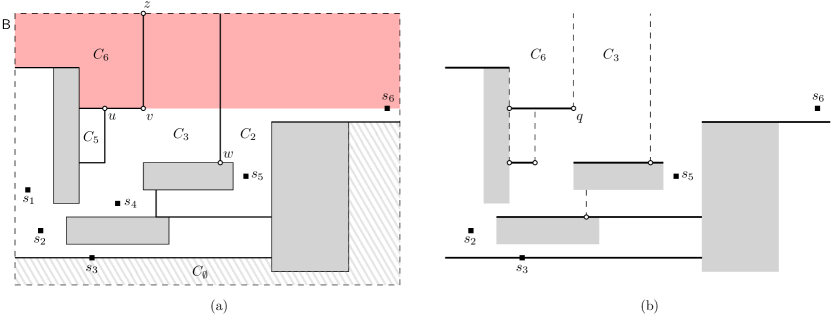
Figure 2: (a) $\mathsf{M}_{y^{+}}$ for $\mathsf{S}=\{s_{1},\ldots,s_{6}\}$ restricted to a box $\mathsf{B}$ with four rectangular holes (gray). $s_{i}$ has a corresponding cell $C_{i}$ for $i=2,3,5,6$ while $s_{1}$ and $s_{4}$ have no cell. A vertical edge $vz$ is from $b(s_{3},s_{6})$ in the (red) region $F(s_{3},s_{6})$. A horizontal edge $uv$ is not part of $b(s_{3},s_{6})$ but it is part of a $b$-edge as no point lying below $uv$ is ${y^{+}}$-reachable from $s_{6}$. (b) Illustration of $\mathsf{Q}_{y^{+}}$ corresponding to $\mathsf{M}_{y^{+}}$. At the boundary point $q$, $d(q,s_{3})=d(q,s_{6})$.

Let $f_{\delta}(p)$ denote the set of farthest sites from a point $p\in\mathsf{F}$ among the sites from which $p$ is $\delta$-reachable for $\delta\in\{{y^{+}},{y^{-}},{x^{+}},{x^{-}}\}$. For each horizontal segment of $\pi_{\mathsf{lu}}(s)\cup\pi_{\mathsf{ru}}(s)$, we call the portion $h$ of the segment such that $f_{y^{+}}(p)=\{s\}$ for any point $p\in h$, a $b$-edge. Observe that no point $p^{\prime}$ with $x_{1}(h)\leq x(p^{\prime})\leq x_{2}(h)$ and $y(p^{\prime})=y(h)-\varepsilon$ for any $\varepsilon>0$ is ${y^{+}}$-reachable from $s$. Thus, a $b$-edge is also an edge of $\mathsf{M}_{y^{+}}$. Since every edge of $\mathsf{M}_{y^{+}}$ is part of a bisector of two sites in $\mathsf{S}$ or a $b$-edge, it is either horizontal or vertical. See Figure 2(a).

Corollary 1.

Every edge of $\mathsf{M}_{y^{+}}$ is an axis-aligned line segment.

For sites contained in a simple polygon, Aronov et al. [4] gave a lemma, called Ordering Lemma, that the order of sites along their convex hull is the same as the order of their Voronoi cells along the boundary of a simple polygon. We give a lemma on the order of sites in the presence of rectangular obstacles. We use it in analyzing the maps and Voronoi diagrams.

Lemma 3.

Let $pq$ be a horizontal segment contained in $\mathsf{F}\setminus C_{\emptyset}$ with $x(p)<x(q)$. For any two sites $f_{p}\in f(p)$ and $f_{q}\in f(q)$ such that $p$ and $q$ are ${y^{+}}$-reachable from both $f_{p}$ and $f_{q}$, if $f_{p}\notin f(q)$ or $f_{q}\notin f(p)$, $x(f_{p})>x(f_{q})$.

Proof.

Ben-Moshe et al. [7] showed that $x(f_{p})\neq x(f_{q})$.

Assume to contrary that $x(f_{p})<x(f_{q})$. Consider two cases that there are (1) two geodesic paths, one from $p$ to $f_{q}$ and one from $q$ to $f_{p}$, intersecting each other at a point, say $r$ (Figure 3(a)), or (2) no two such geodesic paths intersecting each other (Figure 3(b)).

For case (1), we have

$$d(p,f_{q})=d(p,r)+d(r,f_{q})\quad\text{and}\quad d(q,f_{p})=d(q,r)+d(r,f_{p}).$$

We also observe that

$$d(p,f_{p})\leq d(p,r)+d(r,f_{p})\quad\text{and}\quad d(q,f_{q})\leq d(q,r)+d(r,f_{q}).$$

Adding the two inequalities above, we obtain

$$d(p,f_{p})+d(q,f_{q}) \leq d(p,r)+d(r,f_{p})+d(q,r)+d(r,f_{q})$$

$$= d(p,f_{q})+d(q,f_{p}).$$

However, since $f_{p}\notin f(q)$ or $f_{q}\notin f(p)$, we have $d(p,f_{p})+d(q,f_{q})>d(p,f_{q})+d(q,f_{p})$, a contradiction.

Now consider case (2) that there are no two geodesic paths, one from $p$ to $f_{q}$ and one from $q$ to $f_{p}$, intersecting each other (Figure 3(b)). Since $pq$ is horizontal with $x(p)<x(q)$, $x(f_{p})<x(f_{q})$ by assumption, and every geodesic path from $p$ to $f_{q}$ and every geodesic path from $q$ to $f_{p}$ are ${y^{+}}$-monotone, we have $y(f_{p})\neq y(f_{q})$. Without loss of generality, assume $y(f_{p})<y(f_{q})$. Then $\pi_{\mathsf{ru}}(f_{q})$ intersects $\pi(q,f_{p})$ at a point, say $r$ (Figure 3(c)). Since $x(f_{p})<x(f_{q})\leq x(r)$ and $y(f_{p})<y(f_{q})\leq y(r)$, we have $d(r,f_{q})<d(r,f_{p})$, and thus

$$d(q,r)+d(r,f_{q})<d(q,r)+d(r,f_{p})=d(q,f_{p}).$$

Since $d(q,f_{q})\leq d(q,r)+d(r,f_{q})$, we have $d(q,f_{q})<d(q,f_{p})$, a contradiction.

Figure 3: Two cases (a) and (b) for two geodesic path $\pi(p,f_{q})$ and $\pi(q,f_{p})$ when $x(f_{p})<x(f_{q})$. (a) $\pi(p,f_{q})$ and $\pi(q,f_{p})$ intersect each other at $r$. (b) $\pi(p,f_{q})$ and $\pi(q,f_{p})$ do not intersect each other. (c) If $x(f_{p})<x(f_{q})$ and $y(f_{p})\leq y(f_{q})$, $\pi_{\mathsf{ru}}(f_{q})$ intersects $\pi(q,f_{p})$ at $r$.

∎

Since there are at most $m$ sites, we obtain the following corollary from Lemma 3.

Corollary 2.

Any horizontal line segment contained in $\mathsf{F}$ intersects at most $m$ cells in $\mathsf{M}_{y^{+}}$.

Using Corollary 1 and 2, we analyze the complexity of $\mathsf{M}_{y^{+}}$ as follows. Note that each lower endpoint of a vertical edge of $\mathsf{M}_{y^{+}}$ appears on a horizontal line segment passing through a site or the top side of a rectangle. By Corollary 2, the maximal horizontal segment through the top side of a rectangle in $\mathsf{R}$ and contained in $\mathsf{F}$ intersects $O(m)$ vertical edges of $\mathsf{M}_{y^{+}}$. Moreover, the maximal horizontal line segment through a site $s$ and contained in $\mathsf{F}$ intersects $O(1)$ lower endpoints of vertical edges on the boundary of the cell of $s$. Since there are $n$ rectangles in $\mathsf{R}$ and $m$ sites in $\mathsf{S}$, $\mathsf{M}_{y^{+}}$ has $O(nm+m)=O(nm)$ vertical edges. Every horizontal edge of $\mathsf{M}_{y^{+}}$ is a segment of a bisector or a $b$-edge, and it is incident to a side of a rectangle or another vertical edge. Since there are $O(n)$ rectangle sides, and $O(1)$ horizontal edges of $\mathsf{M}_{y^{+}}$ that are incident to a vertical edge, $\mathsf{M}_{y^{+}}$ has $O(n+nm)=O(nm)$ horizontal edges. Thus, $\mathsf{M}_{y^{+}}$ has complexity $O(nm)$.

Now we show that every farthest site $s\in f(p)$ of a point $p$ in $\mathsf{F}$ is one of the farthest sites of $p$ in the four farthest-point maps. By the definition of the farthest-point maps, $p$ is contained in a cell of $\mathsf{M}_{y^{+}}$, $\mathsf{M}_{y^{-}}$, $\mathsf{M}_{x^{+}}$ or $\mathsf{M}_{x^{-}}$. Since every geodesic path connecting two points is either ${y^{+}}$-, ${y^{-}}$-, ${x^{+}}$-, or ${x^{-}}$-monotone by Lemma 1, $s\in f(p)$ is one of the farthest sites of $p$ in the four farthest-point maps. If $p$ is contained in cells of two or more maps, we compare their distances to the farthest sites defining the cells and take the ones with the largest distance as the farthest sites of $p$. Thus, once the four farthest-point maps are constructed, the farthest sites of a query point can be computed from the map.

4 Data Structure for Farthest-neighbor Queries

We present an algorithm that constructs a data structure for farthest site queries. We denote $m$ point sites of $\mathsf{S}$ by $s_{1},\ldots,s_{m}$ such that $x(s_{1})\leq\cdots\leq x(s_{m})$, and $n$ rectangular obstacles of $\mathsf{R}$ by $R_{1},\ldots,R_{n}$. The data structure consists of four parts, each for one axis direction. Since the four parts can be constructed in the same way with respect to their directions, we focus on the part corresponding to the positive $y$-direction, and thus the structure corresponds to $\mathsf{M}_{y^{+}}$. We use $\mathsf{Q}_{y^{+}}$ to denote the query data structure.

By Corollary 1, we can find the farthest site of a query point using a vertical ray shooting query to the horizontal edges of $\mathsf{M}_{y^{+}}$ and a binary search on the lower endpoints of vertical edges of $\mathsf{M}_{y^{+}}$ lying on the horizontal edges of $\mathsf{M}_{y^{+}}$. Thus, we construct $\mathsf{Q}_{y^{+}}$ such that it consists of the horizontal edges of $\mathsf{M}_{y^{+}}$ and the endpoints of vertical edges of $\mathsf{M}_{y^{+}}$ lying on the horizontal edges of $\mathsf{M}_{y^{+}}$.

A point $q$ lying on a horizontal segment $h$ of $\mathsf{Q}_{y^{+}}$ is the lower endpoint of a vertical edge of $\mathsf{M}_{y^{+}}$ if and only if there are two points $q_{1}=(x(q)-\varepsilon,y(q))$ and $q_{2}=(x(q)+\varepsilon,y(q))$ for sufficiently small $\varepsilon>0$ satisfying $f_{y^{+}}(q_{1})\cup f_{y^{+}}(q_{2})=f_{y^{+}}(q)$ and $f_{y^{+}}(q_{1})\neq f_{y^{+}}(q_{2})$. We call each lower endpoint of vertical edges lying on $h$ a boundary point on $h$. See Figure 2(b).

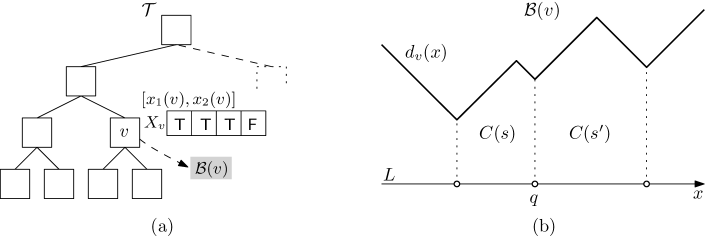
Figure 4: (a) Illustration of a balanced binary search tree $\mathcal{T}$. A node $v$ in $\mathcal{T}$ has domain $[x_{1}(v),x_{2}(v)]$, array $X_{v}$, and a pointer to $\mathcal{B}(v)$. (b) Illustration of $\mathcal{B}(v)$ and $d_{v}(x)$.

We use a plane sweep algorithm with a horizontal sweep line $L$ to construct the horizontal line segments in $\mathsf{Q}_{y^{+}}$. Note that $\mathsf{F}\cap L$ consists of disjoint horizontal segments along $L$. The status of $L$ is the sequence of segments in $\mathsf{F}\cap L$ along $L$. The status changes while $L$ moves upwards over the plane, but not continuously. Each update of the status occurs at a particular $y$-coordinate, which we call an event. To do such updates efficiently, we maintain three data structures for $L$: a balanced binary search tree $\mathcal{T}$ representing the status, a boundary list $\mathcal{B}$, and a list $\mathcal{D}$ of distance functions. The structures $\mathcal{B}$ and $\mathcal{D}$ are associated structures of $\mathcal{T}$.

We store the segments of $\mathsf{F}\cap L$ in a balanced binary search tree $\mathcal{T}$ in increasing order of $x$-coordinate of their left endpoints. Each node $v$ of $\mathcal{T}$ corresponds to a horizontal line segment $h_{v}$ of $\mathsf{F}\cap L$. We store $x_{1}(h_{v})$ and $x_{2}(h_{v})$, and an array $X_{v}$ of $m$ Boolean variables at $v$. We set $X_{v}[i]=\texttt{T}$ if a point on $h_{v}$ is ${y^{+}}$-reachable from $s_{i}$ for $i=1\ldots,m$. Otherwise, we set $X_{v}[i]=\texttt{F}$. The range of $v$ is $[x_{1}(v),x_{2}(v)]$ for $x_{1}(v)=x_{1}(h_{v})$ and $x_{2}(v)=x_{2}(h_{v})$. There are at most $n+1$ nodes in $\mathcal{T}$, and each node maintains an array of size $O(m)$, so $\mathcal{T}$ itself uses $O(nm)$ space in total. See Figure 4(a).

The list $\mathcal{B}$ consists of boundary lists $\mathcal{B}(v)$ for nodes $v$ of $\mathcal{T}$. Each node $v$ of $\mathcal{T}$ has a pointer to its boundary list $\mathcal{B}(v)$, which is a doubly-linked list of the boundary points (including the endpoints of $h_{v}$) lying on $h_{v}$. Each boundary point in $\mathcal{B}$ is the intersection of $L$ and a vertical edge of $\mathsf{M}_{y^{+}}$, so there are $O(nm)$ boundary points in $\mathcal{B}$.

Let $d_{\delta}(p)=d(s,p)$ for a site $s\in f_{\delta}(p)$ if $f_{\delta}(p)\neq\emptyset$, or $d_{\delta}(p)=-\infty$ for $\delta\in\{{y^{+}},{y^{-}},{x^{+}},{x^{-}}\}$. The list $\mathcal{D}$ consists of distance functions $d_{v}$ for nodes $v$ of $\mathcal{T}$. Let ${p}(r)$ denote a point on $L$ with $x({p}(r))=r$ for a real number $r$. Each node $v$ of $\mathcal{T}$ has a pointer to its distance function $d_{v}(x)=d_{y^{+}}({p}(x))$ for $x$ in the range $[x_{1}(v),x_{2}(v)]$ of $v$. It is a piecewise linear function with pieces (segments) of slopes $1$ or $-1$. See Figure 4(b).

There are three types of events: (1) a site event, (2) a bottom-side event, and (3) a top-side event. A site event occurs when $L$ encounters a site in $\mathsf{S}$. A bottom-side event occurs when $L$ encounters the bottom side of a rectangle in $\mathsf{R}$. A top-side event occurs when $L$ encounters the top side of a rectangle in $\mathsf{R}$. Thus, there are $m$ site events, $n$ bottom-side events, and $n$ top-side events. See Figure 5.

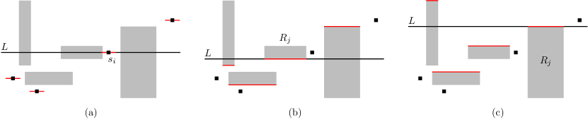
Figure 5: Three types of events. (a) site events. (b) bottom-side events. (c) top-side events.

We maintain and update $\mathcal{T}$, $\mathcal{B}$ and $\mathcal{D}$ during the plane sweep for those events. To handle events, we first sort the events in $y$-coordinate order, which takes $O((n+m)\log(n+m))=O(n\log n+m\log m)$ time. We update $d_{v}(x)$ only at those events and keep it unchanged between two consecutive events. To reflect the distances from sites to ${p}(x)\in h_{v}$ correctly, we assign an additive weight to $d_{v}(x)$, which is the difference in the $y$-coordinates between the current event and the last event at which $d_{v}(x)$ is updated.

Initially, when $L$ is at the bottom side of $\mathsf{B}$, $\mathcal{T}$ consists of one node $v$ with $x_{1}(v)=x_{1}(\mathsf{B})$, $x_{2}(v)=x_{2}(\mathsf{B})$, and $X_{v}[i]=\texttt{F}$ for all $i\in\{1,\ldots,m\}$. $\mathcal{B}(v)$ has no boundary point and $d_{v}(x)=-\infty$ for all $x$, since no points on $L$ is ${y^{+}}$-reachable from any sites.

4.1 Handling a site event

When $L$ encounters a site $s_{i}\in\mathsf{S}$, we find the node $v\in\mathcal{T}$ such that $x_{1}(v)\leq x(s_{i})\leq x_{2}(v)$. Every point on $h_{v}$ is ${y^{+}}$-reachable from $s_{i}$, so we set $X_{v}[i]=\texttt{T}$. We can find $v$ in $O(\log n)$ time, and set $X_{v}[i]=\texttt{T}$ in constant time. Thus, it takes $O(\log n)$ time to update $\mathcal{T}$.

For any point ${p}(x)\in h_{v}$, $d(s_{i},{p}(x))=|x-x(s_{i})|$. By Lemma 3, there is at most one maximal interval $I\subset[x_{1}(v),x_{2}(v)]$ such that $d_{v}(x)<d(s_{i},{p}(x))$ for every $x\in I$. Moreover, $I$ is bounded from left by $x_{1}(v)$ or from right by $x_{2}(v)$ because $d_{v}(x)$ is continuous and consists of pieces (segments) of slopes $1$ or $-1$, and $d(s_{i},{p}(x))=|x-x(s_{i})|$. We find the boundary point ${p}(x^{*})\in h_{v}$ induced by $s_{i}$ such that $d_{v}(x^{*})=d(s_{i},{p}(x^{*}))$. If $I$ is bounded from left, we update $d_{v}(x)$ to $d_{v}(x)=d(s_{i},{p}(x))$ for $x\leq x^{*}$. If $I$ is bounded from right, we update $d_{v}(x)$ to $d_{v}(x)=d(s_{i},{p}(x))$ for $x\geq x^{*}$.

If there is no such point ${p}(x^{*})$, either $d_{v}(x)<d(s_{i},{p}(x))$ or $d_{v}(x)>d(s_{i},{p}(x))$ for all $x$ with $x_{1}(v)\leq x\leq x_{2}(v)$. If $d_{v}(x)<d(s_{i},{p}(x))$, we update $d_{v}(x)$ to $d_{v}(x)=d(s_{i},{p}(x))$ for $x_{1}(v)\leq x\leq x_{2}(v)$. If $d_{v}(x)>d(s_{i},{p}(x))$, we do not update $d_{v}(x)$.

We update $\mathcal{B}(v)$ by removing all the boundary points of $\mathcal{B}(v)$ lying in the interior of $I$ in time linear to the number of the boundary points, and then inserting ${p}(x^{*})$ into $\mathcal{B}(v)$.

Since there are $m$ site events, it takes $O(m\log n)$ time in total to update $\mathcal{T}$. The total time to remove the boundary points is linear to the total number of boundary points in $\mathsf{Q}_{y^{+}}$, which is $O(nm)$.

Lemma 4.

We can handle all site events in $O(nm)$ time using $O(nm)$ space.

4.2 Handling a bottom-side event

When $L$ encounters the bottom side of a rectangle $R\in\mathsf{R}$, the line segment of $\mathsf{F}\cap L$ incident to the bottom side is replaced by two line segments by the event. See Figure 5(b). Thus, we update $\mathcal{T}$ by finding the node $v\in\mathcal{T}$ with $x_{1}(v)\leq x_{1}(R)<x_{2}(R)\leq x_{2}(v)$, removing $v$ from $\mathcal{T}$, and then inserting two new nodes $u$ and $w$ into $\mathcal{T}$. We set $(x_{1}(u),x_{2}(u))=(x_{1}(v),x_{1}(R))$, $(x_{1}(w),x_{2}(w))=(x_{2}(R),x_{2}(v))$, $X_{u}=X_{v}$, and $X_{w}=X_{v}$. This takes $O(\log n)$ time since $\mathcal{T}$ is a balanced binary search tree. It takes $O(m)$ time to copy the Boolean values of $X_{v}$ to $X_{u}$ and $X_{w}$, and to remove $X_{v}$. Thus, it takes $O(m+\log n)$ time to update $\mathcal{T}$.

We update $\mathcal{B}$ by inserting two lists $\mathcal{B}(u)$ and $\mathcal{B}(w)$ into $\mathcal{B}$, copying the boundary points of $\mathcal{B}(v)$ to the lists, and then removing $\mathcal{B}(v)$ from $\mathcal{B}$. By Corollary 2, $h_{v}$ intersects $O(m)$ cells in $\mathsf{M}_{y^{+}}$. Thus, $\mathcal{B}(v)$ has $O(m)$ boundary points, and the update to $\mathcal{B}(u)$ and $\mathcal{B}(w)$ takes $O(m)$ time. There is no change to distance functions.

Since there are $n$ bottom-side events, it takes $O(nm+n\log n)$ time to update $\mathcal{T}$ and $O(nm)$ time to update $\mathcal{B}$ for all bottom-side events.

Lemma 5.

We can handle all bottom-side events in $O(nm+n\log n)$ time using $O(nm)$ space.

4.3 Handling a top-side event

When $L$ encounters the top side of a rectangle $R\in\mathsf{R}$, the two consecutive segments in $\mathsf{F}\cap L$ incident to $R$ are replaced by one segment spanning them by the event. See Figure 5(c). We update $\mathcal{T}$ by finding the two nodes $u,w\in\mathcal{T}$ with $x_{2}(u)=x_{1}(R)$ and $x_{1}(w)=x_{2}(R)$, removing $u$ and $w$ from $\mathcal{T}$, and then inserting a new node $v$ into $\mathcal{T}$. We set $x_{1}(v)=x_{1}(u)$, $x_{2}(v)=x_{2}(w)$, and $X_{v}[i]=X_{u}[i]\vee X_{w}[i]$ for each $i=1,\ldots,m.$ This takes $O(m+\log n)$ time.

We update the distance function $d_{v}(x)$ for $x$ with $x_{1}(v)\leq x\leq x_{1}(R)$ as follows. The geodesic path from any point ${p}(x)\in h_{u}$ to $s_{i}$ with $X_{u}[i]=\texttt{F}$ and $X_{w}[i]=\texttt{T}$ is $xy$-monotone by Lemma 1, and thus $d(s_{i},{p}(x))=y({p}(x))-y(s_{i})+|x(s_{i})-x|$. Also, we observe that $x(s_{i})\geq x$ for any $x$. Thus, every ${p}(x)$ has the same site $s^{*}$ as its farthest site among the sites $s_{i}$ with $X_{u}[i]=\texttt{F}$ and $X_{w}[i]=\texttt{T}$. Then $d(s^{*},{p}(x))=y({p}(x))-y(s^{*})+x(s^{*})-x$. By Lemma 3, there is at most one maximal interval $I$ of $x\in[x_{1}(v),x_{1}(R)]$ such that $d_{v}(x)\leq d(s^{*},{p}(x))$. Moreover, $I$ is bounded from left by $x_{1}(v)$. We find the boundary point ${p}(x^{*})\in h_{u}$ such that $d_{v}(x^{*})=d(s^{*},{p}(x^{*}))$, and update $d_{v}(x)$ to $d(s^{*},{p}(x))$ for $x\leq x^{*}$.

If there is no such point ${p}(x^{*})$, either $d_{v}(x)<d(s^{*},{p}(x))$ or $d_{v}(x)>d(s^{*},{p}(x))$ for all $x$ with $x_{1}(v)\leq x\leq x_{1}(R)$. If $d_{v}(x)<d(s^{*},{p}(x))$, we update $d_{v}(x)$ to $d_{v}(x)=d(s^{*},{p}(x))$ for $x_{1}(v)\leq x\leq x_{1}(R)$. If $d_{v}(x)>d(s^{*},{p}(x))$, we do not update $d_{v}(x)$.

We update $\mathcal{B}[x_{1}(v),x_{1}(R)]$, which is a part of $\mathcal{B}(v)$ with range $[x_{1}(v),x_{1}(R)]$, by removing all the boundary points in the interior of $I$ in time linear to the number of the boundary points, and then inserting ${p}(x^{*})$ as a boundary point. We can handle the case of $x$ with $x_{2}(R)\leq x\leq x_{2}(v)$, and update $\mathcal{B}[x_{2}(R),x_{2}(v)]$ analogously.

4.3.1 Computing distance functions for a top side

We show how to compute $d_{v}(x)$ for $x\in[x_{1}(R),x_{2}(R)]$ and update $\mathcal{B}[x_{1}(R),x_{2}(R)]$ efficiently. Lemma 1 implies the following observation.

Observation 1.

For any point $p$ on the top side of a rectangle $R\in\mathsf{R}$ and any site $s\in\mathsf{S}$ from which $p$ is ${y^{+}}$-reachable, every geodesic path from $p$ to $s$ passes through the top-left corner or the top-right corner of $R$.

For an index $k$, let $\alpha_{k}$ and $\beta_{k}$ denote the top-left corner and the top-right corner of $R_{k}\in\mathsf{R}$, and let $\mathsf{S}_{k}$ denote the set of the sites that lie below the polygonal curve consisting of $\pi_{\mathsf{dl}}(\alpha_{k})$, the top side of $R_{k}$, and $\pi_{\mathsf{dr}}(\beta_{k})$.

For the top-side event of $R=R_{k}$, let $\alpha=\alpha_{k}$ and $\beta=\beta_{k}$. Note that $x(\alpha)=x_{1}(R)$ and $x(\beta)=x_{2}(R)$. Let $\mathsf{S}^{T}$ be the set of the sites $s_{i}$, with $X_{v}[i]=\texttt{T}$ for all $i=1,\ldots,m$. We partition $\mathsf{S}^{T}$ into three disjoint subsets, $\mathsf{S}_{k}$, $\mathsf{S}(\alpha)$, and $\mathsf{S}(\beta)$, such that $\mathsf{S}(\alpha)=\{s_{i}\in\mathsf{S}^{T}\setminus\mathsf{S}_{k}\mid x(s_{i})\leq x_{1}(R)\}$ and $\mathsf{S}(\beta)=\{s_{i}\in\mathsf{S}^{T}\setminus\mathsf{S}_{k}\mid x(s_{i})\geq x_{2}(R)\}$. See Figure 6.

Every geodesic path from any site in $\mathsf{S}(\alpha)$ or $\mathsf{S}(\beta)$ to any point on the top side of $R$ is $xy$-monotone. Thus for any point ${p}(x)$ lying on the top side of $R$, we can compute $d(s^{\alpha},{p}(x))$ and $d(s^{\beta},{p}(x))$, where $s^{\alpha}$ and $s^{\beta}$ are the farthest sites of ${p}(x)$ among sites in $\mathsf{S}(\alpha)$ and among sites in $\mathsf{S}(\beta)$, respectively, as we did for $\mathcal{B}[x_{1}(v),x_{1}(R)]$ or $\mathcal{B}[x_{2}(R),x_{2}(v)]$.

Let $R_{a}$ be the rectangle hit first by the vertical ray emanating from $\alpha$ going downwards, and let $R_{b}$ be the rectangle hit first by the vertical ray emanating from $\beta$ going downwards. See Figure 6.

We compute $d(\alpha,s)$ and $d(\beta,s)$ for each $s\in\mathsf{S}_{k}$, and then compute $d_{v}(x)$ for $x$ with $x_{1}(R)\leq x\leq x_{2}(R)$, where $v$ is the node of $\mathcal{T}$ corresponding to the top-side event of $R$. The top-side events by $R_{a}$ and $R_{b}$ were handled before the top-side event of $R$, and thus we have $d(\alpha_{a},s)$ and $d(\beta_{a},s)$ for sites $s\in\mathsf{S}_{a}$, and $d(\alpha_{b},s^{\prime})$ and $d(\beta_{b},s^{\prime})$ for sites $s^{\prime}\in\mathsf{S}_{b}$. By Observation 1, we can compute $d(\alpha,s)$ and $d(\beta,s)$ for a site $s\in\mathsf{S}_{k}$ as follows.

• If $s\in\mathsf{S}_{a}$, $d(\alpha,s)=\min\{d(\alpha,\alpha_{a})+d(\alpha_{a},s),d(\alpha,\beta_{a})+d(\beta_{a},s)\}$. If $s\notin\mathsf{S}_{a}$, $d(\alpha,s)=|x(\alpha)-x(s)|+|y(\alpha)-y(s)|$ since $\pi(\alpha,s)$ is $xy$-monotone by Lemma 1.

• If $s\in\mathsf{S}_{b}$, $d(\beta,s)=\min\{d(\beta,\alpha_{b})+d(\alpha_{b},s),d(\beta,\beta_{b})+d(\beta_{b},s)\}$. If $s\notin\mathsf{S}_{b}$, $d(\beta,s)=|x(\beta)-x(s)|+|y(\beta)-y(s)|$ since $\pi(\beta,s)$ is $xy$-monotone by Lemma 1.

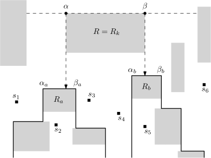
Figure 6: $\mathsf{S}^{T}=\{s_{1},s_{2},s_{3},s_{4},s_{5},s_{6}\}$ is partitioned into $\mathsf{S}_{k}=\{s_{2},s_{3},s_{4},s_{5}\}$, $\mathsf{S}(\alpha)=\{s_{1}\}$, and $\mathsf{S}(\beta)=\{s_{6}\}$. For two rectangles $R_{a}$ and $R_{b}$, $\mathsf{S}_{a}=\{s_{2}\}$ and $\mathsf{S}_{b}=\{s_{5}\}$.

By Observation 1, every geodesic path from $s$ to ${p}(x)$ passes through either $\alpha$ or $\beta$. We denote by $d_{\alpha}(i,x)=d(\alpha,s_{i})+x-x(\alpha)$ the length of a geodesic path from a site $s_{i}$ to ${p}(x)$ passing through $\alpha$, and denote by $d_{\beta}(i,x)=d(\beta,s_{i})+x(\beta)-x$ the length of a geodesic path from $s_{i}$ to ${p}(x)$ passing through $\beta$. Let $D(x)=\max_{s_{i}\in\mathsf{S}_{k}}\min\{d_{\alpha}(i,x),d_{\beta}(i,x)\}$ for all $x$ with $x(\alpha)\leq x\leq x(\beta)$. For ease of description, let $d_{\alpha}(i)=d(\alpha,s_{i})$ and $d_{\beta}(i)=d(\beta,s_{i})+x(\beta)-x(\alpha)$. We observe that $d_{\alpha}(i)\leq d_{\beta}(i)$ for every $s_{i}\in\mathsf{S}_{k}$. Let $d_{\beta\alpha}(i)=d_{\beta}(i)-d_{\alpha}(i)$.

Our goal is to compute $D(x)$ in $O(m)$ time. To achieve this, we consider two cases, either (1) $d_{\beta\alpha}(a)\geq d_{\beta\alpha}(b)$ for every indices $a$ and $b$ with $1\leq a<b\leq m$, or (2) $d_{\beta\alpha}(a)<d_{\beta\alpha}(b)$ for some indices $a$ and $b$ with $1\leq a<b\leq m$. The following two lemmas show how to compute $D(x)$ in $O(m)$ time for these two cases.

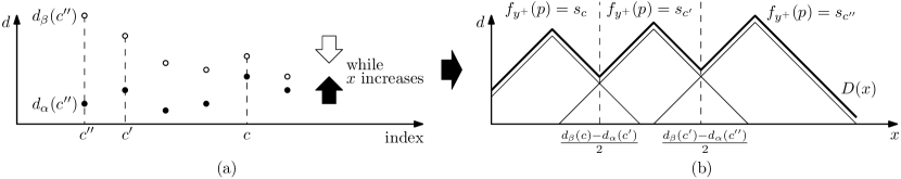
Figure 7: Two graphs showing the distances from sites to ${p}(x)$ for $x_{1}(R)\leq x\leq x_{2}(R)$ with different domains. We find sites $s_{c}=\max_{i\in\{1,\ldots,m\}}d_{\alpha}(i)$, $s_{c^{\prime}}=\max_{i\in\{1,\ldots,c-1\}}d_{\alpha}(i)$, and $s_{c^{\prime\prime}}=\max_{i\in\{1,\ldots,c^{\prime}-1\}}d_{\alpha}(i)$ recursively. They are the farthest sites from ${p}(x)$ moving rightwards. (a) The graph with respect to indices of sites. (b) The graph for $x$ with $x_{1}(R)\leq x\leq x_{2}(R)$.

Lemma 6.

If $d_{\beta\alpha}(a)\geq d_{\beta\alpha}(b)$ for every two indices $a$ and $b$ with $1\leq a<b\leq m$, we can compute $D(x)$ in $O(m)$ time.

Proof.

Let $s_{c}\in f_{y^{+}}(\alpha)$ be the farthest site from $\alpha$ with the smallest index $c$. By Lemma 3 and $x(s_{a})\leq x(s_{b})$ for every two indices $a$ and $b$ with $1\leq a<b\leq m$, no site $s_{i}\not\in f_{y^{+}}(\alpha)$ for any $i=c+1,\ldots,m$ is in $f_{y^{+}}({p}(x))$ for any point ${p}(x)$ on the top side of $R$. Observe that $d_{\alpha}(c)+t\leq d_{\beta}(c)-t$ for $0\leq t\leq d_{\beta\alpha}(c)/2$. Also, $d_{\alpha}(i)+t\leq d_{\beta}(i)-t$ still holds for $0\leq t\leq d_{\beta\alpha}(c)/2$ since $d_{\beta\alpha}(i)\geq d_{\beta\alpha}(c)$ for every index $i=1,\ldots,c-1$.

Let $c^{\prime}$ be the smallest index satisfying $d_{\alpha}(c^{\prime})=\max_{i\in\{1,\ldots,c-1\}}d_{\alpha}(i)$. Then $s_{c^{\prime}}$ is in $f_{y^{+}}({p}(x(\alpha)+t))$ for $t\geq(d_{\beta}(c)-d_{\alpha}(c^{\prime}))/2$. For $d_{\beta\alpha}(c)/2\leq t\leq(d_{\beta}(c)-d_{\alpha}(c^{\prime}))/2$, $s_{c}\in f_{y^{+}}({p}(x(\alpha)+t))$. Therefore, ${p}((d_{\beta}(c)-d_{\alpha}(c^{\prime}))/2)$ becomes a boundary point. See Figure 7. Using $c^{\prime}$, we compute the smallest index $c^{\prime\prime}$ satisfying $d_{\alpha}(c^{\prime})=\max_{i\in\{1,\ldots,c^{\prime}-1\}}d_{\alpha}(i)$ and find all farthest sites $f_{y^{+}}({p}(x(\alpha)+t))$ for all $t$ recursively.

We use a stack storing indices of sites to compute $c^{\prime}$ and $c^{\prime\prime}$ recursively. We can find $s_{c}$ in $O(m)$ time. Let $\mathsf{top}$ be the top element (site) of the stack. Initially, the stack contains $c$. Let $j$ be the index at the $i$-th iteration for $i$ from $c-1$ to $1$. We pop $\mathsf{top}$ from the stack until $d_{\alpha}(j)\geq d_{\alpha}(\mathsf{top})$. Then we push $j$ into the stack if $d_{\alpha}(j)<d_{\alpha}(\mathsf{top})$. Observe that the stack never be empty since $d_{\alpha}(c)>d_{\alpha}(j)$ for all $j\in\{1,\ldots,c-1\}$.

The pseudocode of the algorithm is given in Algorithm 1. We repeat this until we compute $D(x)$ and all boundary points. This takes $O(m)$ time. ∎

Algorithm 1 Computing Farthest Sites on Rectangle

procedure FarthestSites($\{s_{1},\cdots,s_{m}\},R$) $\triangleright$ $x(s_{1})\leq\ldots\leq x(s_{m})$

     $c\leftarrow\operatorname*{arg\,max}_{i\in\{1,\ldots,m\}}d_{\alpha}(i)$ $\triangleright$ $\alpha$ is the top-left corner of $R$

     stack $A\leftarrow\{c\}$

     for $i=c-1$ to $1$ do

         if $d_{\alpha}(i)<d_{\beta}(\mathsf{top}(A))$ then $\triangleright$ $\beta$ is the top-right corner of $R$

              push $i$ into $A$

         else if $d_{\alpha}(i)\geq d_{\alpha}(\mathsf{top}(A))$ then

              while $d_{\alpha}(i)\geq d_{\alpha}(\mathsf{top}(A))$ do

                  pop $\mathsf{top}(A)$ from $A$

              end while

              push $i$ into $A$

         end if

     end for$\triangleright$ $A\neq\emptyset$ during all iterations by $c$.

     sort $A$ in reverse order

     $x\leftarrow x(\alpha)$

     set ${p}(x)$ as a boundary point

     while $|A|>1$ do

         $i\leftarrow\mathsf{top}(A)$

         pop $\mathsf{top}(A)$ from $A$

         $x^{\prime}\leftarrow(d_{\beta}(i)-d_{\alpha}(\mathsf{top}(A)))/2$

         $D(t)\leftarrow\min\{d(\alpha,s_{i})+t-x(\alpha),d(\beta,s_{i})+x(\beta)-t\}$ for $x\leq t\leq x^{\prime}$

         $x\leftarrow x^{\prime}$

         set ${p}(x)$ as a boundary point

     end while

     $x^{\prime}\leftarrow x(\beta)$

     $D(t)\leftarrow\min\{d(\alpha,s_{\mathsf{top}(A)})+t-x(\alpha),d(\beta,s_{\mathsf{top}(A)})+x(\beta)-t\}$ for $x\leq t\leq x^{\prime}$

     set ${p}(x^{\prime})$ as a boundary point

     return $D(x)$ and boundary points

end procedure

If $d_{\beta\alpha}(a)<d_{\beta\alpha}(b)$ for some indices $a$ and $b$ with $a<b$, we can remove either $s_{a}$ or $s_{b}$ by the following lemma.

Lemma 7.

If there are two indices $a$ and $b$ with $a<b$ such that $d_{\beta\alpha}(a)<d_{\beta\alpha}(b)$, either $s_{a}$ or $s_{b}$ is a farthest site from no point ${p}(x)$ for $x$ with $x_{1}(R)\leq x\leq x_{2}(R)$.

Proof.

The proof is similar to that of Lemma 3. First, we show that if there are two geodesic paths $\pi(\alpha,s_{b})$ and $\pi(\beta,s_{a})$ that intersect each other, then $d_{\beta\alpha}(a)\geq d_{\beta\alpha}(b)$. Let $q$ be a point in the intersection of the paths. Then

$$d(\alpha,s_{b})=d(\alpha,q)+d(q,s_{b})\quad\text{and}\quad d(\beta,s_{a})=d(\beta,q)+d(q,s_{a}).$$

We observe that $d(\alpha,s_{a})\leq d(\alpha,q)+d(q,s_{a})$ and $d(\beta,s_{b})\leq d(\beta,q)+d(q,s_{b})$. Adding these two inequalities, we obtain

$$d(\alpha,s_{a})+d(\beta,s_{b}) \leq d(\alpha,q)+d(q,s_{b})+d(\beta,q)+d(q,s_{a})$$

$$= d(\alpha,s_{b})+d(\beta,s_{a})$$

and thus, $d(\beta,s_{b})-d(\alpha,s_{b})\leq d(\beta,s_{a})-d(\alpha,s_{a})$. Since $d(\beta,s_{b})-d(\alpha,s_{b})=d_{\beta}(b)+C-d_{\alpha}(b)$ and $d(\beta,s_{a})-d(\alpha,s_{a})=d_{\beta}(a)+C-d_{\alpha}(a)$, we have $d_{\beta}(b)-d_{\alpha}(b)\leq d_{\beta}(a)-d_{\alpha}(a)$, where $C=x(\beta)-x(\alpha)$. Therefore, $d_{\beta\alpha}(a)\geq d_{\beta\alpha}(b)$.

By contraposition, if $d_{\beta\alpha}(a)<d_{\beta\alpha}(b)$, no two geodesic paths $\pi(\alpha,s_{b})$ and $\pi(\beta,s_{a})$ intersect each other. Since $y(\alpha)=y(\beta)$, $x(s_{a})\leq x(s_{b})$, and all geodesic paths from the sites we consider are ${y^{+}}$-monotone, $y(s_{a})\neq y(s_{b})$. We show that $s_{b}$ is a farthest site from no point ${p}(x)$ if $y(s_{a})<y(s_{b})$, and $s_{a}$ is a farthest site from no point ${p}(x)$ if $y(s_{a})>y(s_{b})$.

Consider the case that $y(s_{a})<y(s_{b})$. Then $\pi_{\mathsf{ru}}(s_{b})$ intersects $\pi(\beta,s_{a})$ at a point, say $q$. Since $x(s_{a})\leq x(s_{b})\leq x(q)$, $y(s_{a})<y(s_{b})\leq y(q)$, and $\pi(q,s_{b})$ is $xy$-monotone, $d(q,s_{a})>d(q,s_{b})$. Then

$$d(\beta,s_{b})\leq d(\beta,q)+d(q,s_{b})<d(\beta,q)+d(q,s_{a})=d(\beta,s_{a})\quad\text{and}\quad d(\beta,s_{b})-d(\beta,s_{a})<0.$$

Then $d_{\beta}(b)-d_{\beta}(a)<0$ because $d_{\beta}(b)=d(\beta,s_{b})+C$ and $d_{\beta}(a)=d(\beta,s_{a})+C$, where $C=x(\beta)-x(\alpha)$. Since $d_{\beta\alpha}(a)<d_{\beta\alpha}(b)$, we have $d_{\alpha}(b)-d_{\alpha}(a)<d_{\beta}(b)-d_{\beta}(a)<0$, $d_{\alpha}(b)<d_{\alpha}(a)$ and $d_{\beta}(b)<d_{\beta}(a)$. This implies that

$$\min\{d_{\alpha}(b)+t,d_{\beta}(b)-t\}<\min\{d_{\alpha}(a)+t,d_{\beta}(a)-t\}\quad\text{for any }t\in[0,x(\beta)-x(\alpha)].$$

Thus, $s_{b}$ is a farthest site from no point ${p}(x)$.

Now consider the case that $y(s_{a})>y(s_{b})$. Then $\pi_{\mathsf{lu}}(s_{a})$ intersects $\pi(\alpha,s_{b})$ at a point, say $q^{\prime}$. Since $x(q^{\prime})\leq x(s_{a})\leq x(s_{b})$, $y(q^{\prime})\geq y(s_{a})>y(s_{b})$, and $\pi(q^{\prime},s_{a})$ is $xy$-monotone, $d(q^{\prime},s_{b})>d(q^{\prime},s_{a})$. Thus,

$$d_{\alpha}(a)\leq d(\alpha,q^{\prime})+d(q^{\prime},s_{a})<d(\alpha,q^{\prime})+d(q^{\prime},s_{b})=d_{\alpha}(b)\quad\text{and}\quad d_{\alpha}(b)-d_{\alpha}(a)>0.$$

Since $d_{\beta\alpha}(a)<d_{\beta\alpha}(b)$, we have $0<d_{\alpha}(b)-d_{\alpha}(a)<d_{\beta}(b)-d_{\beta}(a)$. Then $d_{\beta}(b)>d_{\beta}(a)$ and $d_{\alpha}(b)>d_{\alpha}(a)$ which implies that

$$\min\{d_{\alpha}(b)+t,d_{\beta}(b)-t\}>\min\{d_{\alpha}(a)+t,d_{\beta}(a)-t\}\quad\text{for any }t\in[0,x(\beta)-x(\alpha)].$$

Therefore, $s_{a}$ is a farthest site from no point ${p}(x)$. ∎

Algorithm 2 Pruning Sites on Rectangle

procedure PruningSites($\{s_{1},\ldots,s_{m}\},R$) $\triangleright$ $x(s_{1})\leq\ldots\leq x(s_{m})$

     stack $A\leftarrow\emptyset$ $\triangleright$ $\alpha$ is the top-left corner of $R$

     for $i=1$ to $m$ do $\triangleright$ $\beta$ is the top-right corner of $R$

         while True do

              if $A=\emptyset$ or $d(\beta,s_{i})-d(\alpha,s_{i})\geq d(\beta,\mathsf{top}(A))-d(\alpha,\mathsf{top}(A))$ then

                  push $s_{i}$ into $A$

                  break

              else if $d(\alpha,s_{i})\leq d(\alpha,\mathsf{top}(A))$ then

                  ignore $s_{i}$

                  break

              else if $d(\alpha,s_{i})>d(\alpha,\mathsf{top}(A))$ then

                  pop $\mathsf{top}(A)$ from $A$

              end if

         end while

     end for

     call FarthestSites($A,R$)

end procedure

Lemmas 6 and 7 imply that the complexity of $D(x)$ is $O(m)$. By Lemma 7, we can remove the sites which never be the farthest sites by comparing $d_{\beta\alpha}(a)$ and $d_{\beta\alpha}(b)$ for two indices $a$ and $b$. This can be done in $O(m)$ time by Algorithm 2. After pruning, $d_{\beta\alpha}(a)\geq d_{\beta\alpha}(b)$ for every pair of remaining sites $s_{a}$ and $s_{b}$ with $a<b$. Therefore, we can compute $D(x)$ in $O(m)$ time by Lemma 6. Then we can compute $d_{v}(x)=\max\{d(s^{\alpha},{p}(x)),D(x),d(s^{\beta},{p}(x))\}$. in $O(m)$ time. We update $\mathcal{B}[x_{1}(R),x_{2}(R)]$ in $O(m)$ time using $d_{v}(x)$.

There are $n$ top-side events, so we can handle the top-side events in $O(nm+n\log n)$ time. In addition, we compute distances from $O(m)$ sites to each corner of $O(n)$ rectangles, and store them. Using ray shooting queries emanating from the corners of rectangles, it takes $O(nm)+O(n\log n)$ time using $O(nm)$ space. Therefore, we have the following lemma.

Lemma 8.

We can handle all top-side events in $O(nm+n\log n)$ time using $O(nm)$ space.

4.4 Constructing the query data structure

Initially, $\mathsf{Q}_{y^{+}}=\emptyset$. For each site event and top-side event, we update $d_{v}(x)$ and $\mathcal{B}(v)$ for node $v$ of $\mathcal{T}$ corresponding to the event. We insert a horizontal segment $h$ corresponding to each interval which is updated at the event into $\mathsf{Q}_{y^{+}}$, and copy the boundary points into $h$. For each site event, at most one horizontal line segment $h$ is inserted. There is no boundary point in the interior of $h$, so we can copy $h$ with two endpoints in $O(1)$ time. For each top-side event, at most three horizontal line segments are inserted. They have $O(m)$ boundary points by Lemma 3, so we can copy them in $O(m)$ time. There are $O(n+m)$ horizontal segments and $O(nm)$ boundary points in $\mathsf{Q}_{y^{+}}$, so the query structure $\mathsf{Q}_{y^{+}}$ uses $O(nm)$ space.

4.4.1 Farthest-point queries

Once $\mathsf{Q}_{y^{+}}$ is constructed, we can find $f_{y^{+}}(q)$ from a query point $q\in\mathsf{F}\setminus C_{\emptyset}$. We find the farthest sites from $q$ in the other three maps using their query data structures.

By Corollary 1, our query problem reduces to the vertical ray shooting queries. We use the data structure by Giora and Kaplan [15] for vertical ray shooting queries on $O(n+m)$ horizontal line segments in $\mathsf{Q}_{y^{+}}$, which requires $O((n+m)\log(n+m))$ time and $O(n+m)$ space for construction. Let $h$ be the horizontal segment in $\mathsf{Q}_{y^{+}}$ hit first by the vertical ray emanating from $q$ going downwards. We can find $h$ in $O(\log(n+m))$ time using the ray shooting structure. If no horizontal segment in $\mathsf{Q}_{y^{+}}$ is hit by the ray, $q$ is ${y^{+}}$-reachable from no site. Otherwise, there are $O(m)$ boundary points on $h$, sorted in increasing order of $x$-coordinate. With those boundary points, we can find $f(q)$ for a query point $q$ in $O(\log m)$ time using binary search. Thus, a farthest-neighbor query takes $O(\log(n+m))$ time in total.

Once the farthest sites of $q$ for each of the four data structures is found, we take the sites with the largest distance among them as the farthest sites $f(q)$ of $\mathsf{S}$ from $q$. Combining Lemmas 4, 5 and 8 with query time, we have the following theorem.

Theorem 1.

We can construct a data structure for $m$ point sites in the presence of $n$ axis-aligned rectangular obstacles in the plane in $O(nm+n\log n+m\log m)$ time and $O(nm)$ space that answers any $L_{1}$ farthest-neighbor query in $O(\log(n+m))$ time.

5 Computing the Explicit Farthest-point Voronoi Diagram

We construct the explicit farthest-point Voronoi diagram $\mathsf{FVD}=\mathsf{FVD}(\mathsf{S},\mathsf{R})$ of a set $\mathsf{S}$ of $m$ point sites in the presence of a set $\mathsf{R}$ of $n$ rectangular obstacles in the plane. It is known that $\mathsf{FVD}$ requires $\Omega(nm)$ space [5, 7]. It takes $\Omega(n\log n)$ time to compute the geodesic distance between two points in $\mathsf{F}$ [12]. By a reduction from the sorting problem, it can be shown to take $\Omega(m\log m)$ time for computing the farthest-point Voronoi diagram of $m$ point sites in the plane. We present an $O(nm+n\log n+m\log m)$-time algorithm using $O(nm)$ space that matches the time and space lower bounds. This is the first optimal algorithm for constructing the farthest-point Voronoi diagram of points in the presence of obstacles in the plane in both time and space.

We construct $\mathsf{Q}_{y^{+}}$ using the plane sweep in Section 4. During the plane sweep, we find all horizontal edges of $\mathsf{M}_{y^{+}}$ and insert them into $\mathsf{Q}_{y^{+}}$ as segments. We find all the lower endpoints of the vertical edges of $\mathsf{M}_{y^{+}}$ and insert them as boundary points in $\mathcal{B}$. We also find the upper endpoints of vertical edges of $\mathsf{M}_{y^{+}}$. By connecting those endpoints using vertical segments appropriately, we can construct $\mathsf{M}_{y^{+}}$ from $\mathsf{Q}_{y^{+}}$ in a doubly connected edge list without increasing the time and space complexities. The other three maps can also be constructed in the same way in the same time and space.

We construct the farthest-point Voronoi diagram $\mathsf{FVD}$ using the four maps explicitly. Note that $f(p)=f_{{y^{+}}}(p)$ for any point $p$ lying on the top side of $\mathsf{B}$. Thus, it suffices to compute $\mathsf{FVD}$ in $\mathsf{F}\cap\mathsf{B}$. For ease of description, we assume that the $x$-coordinates of the rectangles in $\mathsf{R}$ are all distinct. We consider a vertical decomposition $\mathsf{F}_{V}$ obtained by drawing maximal vertical line segments contained in $\mathsf{F}\cap\mathsf{B}$ of which each is extended from a vertical side of a hole of $\mathsf{F}$. Let $V$ be a set of such vertical line segments. $\mathsf{F}\setminus\bigcup_{\ell\in V}\ell$ consists of $O(n)$ connected faces. Each face is a rectangle since each hole of $\mathsf{F}$ is a rectangle and $\mathsf{F}$ is bounded by $\mathsf{B}$. See Figure 8(a).

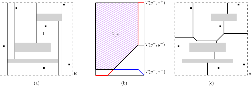
Figure 8: (a) Vertical decomposition $\mathsf{F}_{V}$. $\mathsf{f}$ is a face of $\mathsf{F}_{V}$. (b) $Z_{y^{+}}$ is a region in $\mathsf{f}$ above the upper envelope of three traces, $T({y^{+}},{y^{-}})$, $T({y^{+}},{x^{+}})$ and $T({y^{+}},{x^{-}})$. (c) Explicit geodesic $L_{1}$ farthest-point Voronoi diagram $\mathsf{FVD}$.

Any two farthest-point maps $\mathsf{M}_{1},\mathsf{M}_{2}$ have a bisector which consists of the points in $\mathsf{F}$ having the same distance to their farthest sites in $\mathsf{M}_{1}$ and in $\mathsf{M}_{2}$. The four maps define six bisectors. In a face of $\mathsf{F}_{V}$, the six bisectors and some axis-aligned segments partition the face into zones such that $\mathsf{FVD}$ restricted to one zone coincides with the diagram in the corresponding region of a farthest-point map. Thus, we compute the bisectors between maps in each face of $\mathsf{F}_{V}$, partition the face into zones, find the region of a farthest-point map corresponding to each zone, and then glue the regions and faces to compute $\mathsf{FVD}$ completely.

5.1 Bisectors of farthest-point maps

We define the bisector between $\mathsf{M}_{\delta}$ and $\mathsf{M}_{\delta^{\prime}}$ as $B(\delta,\delta^{\prime})=\{q\in\mathsf{F}\mid d_{\delta}(q)=d_{\delta^{\prime}}(q)\}$ for any two distinct $\delta,\delta^{\prime}\in\{{y^{+}},{y^{-}},{x^{+}},{x^{-}}\}$. We show some structural and combinatorial properties of the bisectors between two farthest-point maps.

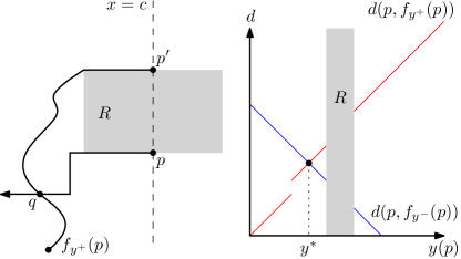
Figure 9: Proof of Lemma 9. $d(p,f_{y^{+}}(p))$ can be discontinuous, but it is increasing. $d(p,f_{y^{-}}(p))$ can be discontinuous, but it is decreasing. At $p^{*}$ with $y(p^{*})=y^{*}$, $d(p^{*},f_{y^{+}}(p^{*}))=d(p^{*},f_{y^{-}}(p^{*}))$ and $p^{*}$ is in $B({y^{+}},{y^{-}})$.

Lemma 9.

Any vertical line intersects $B({y^{+}},{y^{-}})$ in at most one point.

Proof.

Imagine that a point $p$ moves vertically upwards. We show that $d_{y^{+}}(p)$ increases as $p$ moves. By Corollary 1, $f_{y^{+}}(p)$ does not change until $p$ meets a horizontal edge of $\mathsf{M}_{y^{+}}$, or a rectangle of $\mathsf{R}$, and thus $d_{y^{+}}(p)$ increases as $p$ moves. When $p$ meets a horizontal edge of $\mathsf{M}_{y^{+}}$, $f_{y^{+}}(p)$ changes, but $d_{y^{+}}(p)$ still increases by the definition of $f_{y^{+}}(p)$.

Consider the case that $p$ meets the bottom side of a rectangle $R\in\mathsf{R}$. See Figure 9. Let $p^{\prime}$ be the point on the top side of $R$ with $x(p^{\prime})=x(p)$. Then there is a geodesic path $\pi(p^{\prime},f_{y^{+}}(p))$ that passes through the top-left (or the top-right) corner of $R$. Without loss of generality, assume it passes the top-left corner of $R$. By the definition of $f_{y^{+}}(p)$, $\pi_{\mathsf{ld}}(p)$ intersects $\pi(p^{\prime},f_{y^{+}}(p))$ at a point, say $q$. Then,

$$d(p,f_{y^{+}}(p))\leq d(p,q)+d(q,f_{y^{+}}(p))<d(p^{\prime},f_{y^{+}}(p))\leq d(p^{\prime},f_{y^{+}}(p^{\prime})).$$

Therefore, $d(p,f_{y^{+}}(p))$ still increases as $p$ jumps to $p^{\prime}$. Likewise, $d(p,f_{y^{-}}(p))$ decreases as $p$ moves vertically upwards. Then $d(p,f_{y^{+}}(p))=d(p,f_{y^{-}}(p))$ occurs at most once at a moment for $p$ moving vertically upwards. Thus, any vertical line intersects $B({y^{+}},{y^{-}})$ in at most one point. ∎

By Lemma 9, $B({y^{+}},{y^{-}})$ is $x$-monotone consisting of segments of slopes $0$, $+1$, or $-1$.

Lemma 10.

For any vertical line segment $\ell$ contained in $\mathsf{F}$, $\ell\cap B({y^{+}},{x^{+}})$ consists of at most one connected component.

Proof.

The proof is similar to the one for Lemma 9. Consider a vertical line segment $\ell$ contained in $\mathsf{F}$. Imagine that a point $p$ moves vertically upwards from the lower endpoint of $\ell$ to the upper endpoint. We show that $d_{y^{+}}(p)-y(p)=d_{1}(p)$ does not decrease. By Corollary 1, $f_{y^{+}}(p)$ does not change until $p$ meets a horizontal edge of $\mathsf{M}_{y^{+}}$, or a rectangle of $\mathsf{R}$, and thus $d_{1}(p)$ remains the same as $p$ moves. When $p$ meets a horizontal edge of $\mathsf{M}_{y^{+}}$, $f_{y^{+}}(p)$ changes and $d_{1}(p)$ increases by the definition of $f_{y^{+}}(p)$.

We also show that $d_{x^{+}}(p)-y(p)=d_{2}(p)$ does not increase. Recall that every distance function in $\mathcal{D}$ consists of pieces of slopes $1$ or $-1$ during the plane sweep in Section 4. Therefore, $d_{2}(p)$ does not increase. Thus there is at most one connected component satisfying $d_{y^{+}}(p)=d_{x^{+}}(p)$ in $\ell$. ∎

We can also show that Lemma 10 holds for $B({y^{+}},{x^{-}})$. See Figure 10 for bisectors. Lemmas 9 and 10 imply that $f(p^{\prime})=f_{y^{+}}(p^{\prime})$ if $p^{\prime}p$ is a vertical line segment contained in $\mathsf{F}$ with $y(p^{\prime})>y(p)$, and $f(p)=f_{y^{+}}(p)$. Thus, these three bisectors contained in a face of $\mathsf{F}_{V}$ are $x$-monotone.

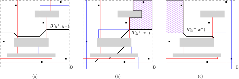
Figure 10: Three bisectors of $\mathsf{M}_{y^{+}}$ (red) and the other three farthest-point maps (blue). (a) $B({y^{+}},{y^{-}})$. (b) $B({y^{+}},{x^{+}})$. (c) $B({y^{+}},{x^{-}})$. Bisectors may contain a two-dimensional region.

For each face $\mathsf{f}$ of $\mathsf{F}_{V}$, we compute the portion of $B({y^{+}},{y^{-}})$ contained in $\mathsf{f}$. As $B({y^{+}},{y^{-}})\cap\mathsf{f}$ is $x$-monotone, we sweep a vertical line $L$ from $x_{1}(\mathsf{f})$ to $x_{2}(\mathsf{f})$ maintaining a point $p\in\mathsf{f}\cap L$ with $d_{y^{+}}(p)=d_{y^{-}}(p)$. First, we compute $p$ lying on the left side of $\mathsf{f}$ as follows. There are $O(m)$ intersections of the left side of $\mathsf{f}$ with the horizontal segments of $\mathsf{Q}_{y^{+}}$ and $\mathsf{Q}_{y^{-}}$ as any vertical line segment contained in $\mathsf{F}$ intersects $O(m)$ horizontal segments of them. For each intersection point $q$, we compute $d_{y^{+}}(q)$ and $d_{y^{-}}(q)$, and find two consecutive points $q_{1}$ and $q_{2}$ among the intersection points by $y$-coordinate such that $d_{y^{+}}(q_{1})\leq d_{y^{-}}(q_{1})$ and $d_{y^{-}}(q_{2})\leq d_{y^{+}}(q_{2})$. We can compute $q_{1}$ and $q_{2}$ in $O(m)$ time using $\mathsf{Q}_{y^{+}}$ and $\mathsf{Q}_{y^{-}}$. Then we compute $p$ lying on $q_{1}q_{2}$.

Having the distance functions, we have the slope of the bisector incident to $p$. Let $\vec{\ell}$ be the half-line from $p$ with the slope going rightward. We find the first point $p^{\prime}$ on $\vec{\ell}$ from $p$ at which the slope of $d_{y^{+}}(p^{\prime})$ or $d_{y^{-}}(p^{\prime})$ changes. Since the slope of $d_{y^{+}}(p^{\prime})$ changes at most once within a cell of $\mathsf{M}_{y^{+}}$, we can find $p^{\prime}$ in time linear to the complexity of the cells containing $p$ of the maps. If there are two or more such points, $p$ is the point with the maximum $y$-coordinate among them.

There may be no point $p$ satisfying $d_{y^{+}}(p)=d_{y^{-}}(p)$ if there is a point $q\in\mathsf{f}\cap L$ such that $d_{y^{+}}(q^{\prime})>d_{y^{-}}(q^{\prime})$ for every point $q^{\prime}$ lying above $q$, and $d_{y^{+}}(q^{\prime})<d_{y^{-}}(q^{\prime})$ for every point $q^{\prime}$ lying below $q$. We maintain the point $q$ in this case. Note that $q$ follows a horizontal segment during the plane sweep, and thus we can find the first point $p$ with $d_{y^{+}}(p)=d_{y^{-}}(p)$ using a horizontal half-line from $q$.

During the plane sweep, $p$ or $q$ moves along $B({y^{+}},{y^{-}})$ rightwards until it meets the right side of $\mathsf{f}$. We compute the other bisectors in $\mathsf{f}$ similarly.

We compute the trace $T({y^{+}},{y^{-}})$ of $p$ and $q$ during the sweep. Observe that every vertical line intersecting $\mathsf{f}$ also intersects the trace in one point $t$. Moreover, if the line intersects $B({y^{+}},{y^{-}})\cap\mathsf{f}$, $t$ is the topmost point of the intersection. Since we have $\mathsf{M}_{x^{+}}$ and $\mathsf{M}_{x^{-}}$, we can compute the two traces $T({y^{+}},{x^{+}})$ and $T({y^{+}},{x^{-}})$ similarly.

We observe that each bisector and trace in $\mathsf{f}$ has $O(m)$ complexity. We get the distance functions using $\mathsf{Q}_{y^{+}}$, $\mathsf{Q}_{y^{-}}$, $\mathsf{Q}_{x^{+}}$, and $\mathsf{Q}_{x^{-}}$ which consist of $O(n+m)$ line segments and support $O(\log(n+m))$ query time. After computing those distance functions, the traces can be constructed in time linear to their complexities. Thus, in total it takes $O(nm+n\log n+m\log m)$ time to construct the traces for all faces.

5.2 Partitioning $\mathsf{f}$ into zones

With the three traces $T({y^{+}},{y^{-}})$, $T({y^{+}},{x^{+}})$, $T({y^{+}},{x^{-}})$ in $\mathsf{f}$, we compute the zone $Z_{y^{+}}$ in $\mathsf{f}$ corresponding to $\mathsf{M}_{y^{+}}$ in $\mathsf{f}$. Let $T$ be an upper envelope of $T({y^{+}},{y^{-}})$, $T({y^{+}},{x^{+}})$ and $T({y^{+}},{x^{-}})$. Then $Z_{y^{+}}$ is the set of points lying above $T$ in $\mathsf{f}$. See Figure 8(b). The following lemma can be shown using the lemmas in Appendix LABEL:apx:pro.bisectors.

Lemma 11.

For any point $p\in Z_{y^{+}}$, $f(p)=f_{y^{+}}(p)$.

Similarly, we define the other three zones $Z_{y^{-}}$, $Z_{x^{+}}$, and $Z_{x^{-}}$. Note that $d_{\delta}(p)>d_{\delta^{\prime}}(p)$ for every point $p\in Z_{\delta}$ for distinct $\delta,\delta^{\prime}\in\{{y^{+}},{y^{-}},{x^{+}},{x^{-}}\}$. By Lemma 11, $\mathsf{FVD}\cap Z_{{y^{+}}}$ coincides with $\mathsf{M}_{y^{+}}$. We copy the corresponding farthest-point map of $\delta$ into $Z_{\delta}$ for each $\delta\in\{{y^{+}},{y^{-}},{x^{+}},{x^{-}}\}$.

We call $\mathsf{f}\setminus(Z_{y^{+}}\cup Z_{y^{-}}\cup Z_{x^{+}}\cup Z_{x^{-}})$ the bisector zone. Every point $p$ in the bisector zone lies on a bisector of two or more maps. Thus, for each bisector of two maps, we copy one of the maps into the corresponding zone.

5.3 Gluing along boundaries

We first glue the zones along their boundaries in each face of $\mathsf{F}_{V}$. For each edge $e$ incident to two zones, we check whether the two cells incident to the edge have the same farthest site or not. If they have the same farthest site, $e$ is not a Voronoi edge of $\mathsf{FVD}$. Then we remove the edge and merge the cells into one. If they have different farthest sites, $e$ is a Voronoi edge of $\mathsf{FVD}$. This takes $O(nm)$ time in total, which is linear to the number of Voronoi edges and cells in $\mathsf{FVD}$.

After gluing zones in every face, we glue the faces of $\mathsf{F}_{V}$ along their boundaries. Since $e$ is a vertical line segment and incident to more than two cells, we divide $e$ into pieces such that any point in the same piece $e^{\prime}$ is incident to the same set of two cells. If both cells incident to $e^{\prime}$ have the same farthest site, $e^{\prime}$ is not a Voronoi edge of $\mathsf{FVD}$. Then we remove the edge and merge the cells. If they have different farthest sites, $e^{\prime}$ is a Voronoi edge of $\mathsf{FVD}$. There are $O(n)$ vertical line segments in $V$ and each of them intersects $O(m)$ cells of $\mathsf{FVD}$, so it takes $O(nm)$ time in total. Then we obtain the geodesic $L_{1}$ farthest-point Voronoi diagram $\mathsf{FVD}$ explicitly. See Figure 8(c).

Theorem 2.

We can compute the $L_{1}$ farthest-point Voronoi diagram of $m$ point sites in the presence of $n$ axis-aligned rectangular obstacles in the plane in $O(nm+n\log n+m\log m)$ time and $O(nm)$ space.

Corollary 3.

We can compute the $L_{1}$ geodesic center of $m$ point sites in the presence of $n$ axis-aligned rectangular obstacles in the plane in $O(nm+n\log n+m\log m)$ time and $O(nm)$ space.

6 Concluding Remarks

We present an optimal algorithm for computing the farthest-point Voronoi diagram of point sites in the presence of rectangular obstacles. However, our algorithm may not work for more general obstacles as it is, because some properties we use for the axis-aligned rectangles including their convexity may not hold any longer. Our results, however, may serve as a stepping stone to closing the gap to the optimal bounds.

References

- [1] A. Aggarwal, L.J. Guibas, J. Saxe, and P.W. Shor. A linear-time algorithm for computing the Voronoi diagram of a convex polygon. Discrete & Computational Geometry, 4(6):591–604, 1989.
- [2] H. Alt, O. Cheong, and A. Vigneron. The Voronoi diagram of curved objects. Discrete & Computational Geometry, 34(3):439–453, 2005.
- [3] B. Aronov. On the geodesic Voronoi diagram of point sites in a simple polygon. Algorithmica, 4(1):109–140, 1989.
- [4] B. Aronov, S. Fortune, and G. Wilfong. The furthest-site geodesic Voronoi diagram. Discrete & Computational Geometry, 9(3):217–255, 1993.
- [5] S.W. Bae and K.-Y. Chwa. The geodesic farthest-site Voronoi diagram in a polygonal domain with holes. In Proceedings of the 25th Annual Symposium on Computational Geometry (SoCG), pages 198–207, 2009.
- [6] B. Ben-Moshe, B.K. Bhattacharya, and Q. Shi. Farthest neighbor Voronoi diagram in the presence of rectangular obstacles. In Proceedings of the 13th Canadian Conference on Computational Geometry (CCCG), pages 243–246, 2005.
- [7] B. Ben-Moshe, M.J. Katz, and J.S.B. Mitchell. Farthest neighbors and center points in the presence of rectangular obstacles. In Proceedings of the 17th Annual Symposium on Computational Geometry (SoCG), pages 164–171, 2001.
- [8] O. Cheong, H. Everett, M. Glisse, J. Gudmundsson, S. Hornus, S. Lazard, M. Lee, and H.-S. Na. Farthest-polygon Voronoi diagrams. Computational Geometry, 44(4):234–247, 2011.
- [9] L.P. Chew and R.L. Dyrsdale III. Voronoi diagrams based on convex distance functions. In Proceedings of the 1st annual symposium on Computational geometry (SoCG), pages 235–244, 1985.
- [10] J. Choi, C.-S. Shin, and S.K. Kim. Computing weighted rectilinear median and center set in the presence of obstacles. In International Symposium on Algorithms and Computation, pages 30–40. Springer, 1998.
- [11] J. Choi and C. Yap. Monotonicity of rectilinear geodesics in -space. In Proceedings of the 12th Annual Symposium on Computational Geometry (SoCG), pages 339–348, 1996.
- [12] P.J. De Rezende, D.-T. Lee, and Y.-F. Wu. Rectilinear shortest paths with rectangular barriers. In Proceedings of the 1st Annual Symposium on Computational Geometry (SoCG), pages 204–213, 1985.
- [13] H. Edelsbrunner and R. Seidel. Voronoi diagrams and arrangements. Discrete & Computational Geometry, 1(1):25–44, 1986.
- [14] S. Fortune. A sweepline algorithm for Voronoi diagrams. Algorithmica, 2(1):153–174, 1987.
- [15] Y. Giora and H. Kaplan. Optimal dynamic vertical ray shooting in rectilinear planar subdivisions. ACM Transactions on Algorithms, 5(3):28:1–51, 2009.
- [16] J. Hershberger and S. Suri. An optimal algorithm for Euclidean shortest paths in the plane. SIAM Journal on Computing, 28(6):2215–2256, 1999.
- [17] R. Klein. Abstract Voronoi diagrams and their applications. In Proceedings of the 4th International Workshop on Computational Geometry (EuroCG), pages 148–157. Springer, 1988.
- [18] D.-T. Lee. Two-dimensional Voronoi diagrams in the -metric. Journal of the ACM, 27(4):604–618, 1980.
- [19] J.S.B. Mitchell. shortest paths among polygonal obstacles in the plane. Algorithmica, 8(1–6):55–88, 1992.
- [20] E. Oh. Optimal algorithm for geodesic nearest-point Voronoi diagrams in simple polygons. In Proceedings of the 30th Annual ACM-SIAM Symposium on Discrete Algorithms (SODA), pages 391–409, 2019.
- [21] E. Oh and H.-K. Ahn. Voronoi diagrams for a moderate-sized point-set in a simple polygon. Discrete & Computational Geometry, 63(2):418–454, 2020.
- [22] E. Oh, L. Barba, and H.-K. Ahn. The geodesic farthest-point Voronoi diagram in a simple polygon. Algorithmica, 82(5):1434–1473, 2020.
- [23] E. Papadopoulou and S.K. Dey. On the farthest line-segment Voronoi diagram. International Journal of Computational Geometry & Applications, 23(06):443–459, 2013.
- [24] E. Papadopoulou and D.T. Lee. The Voronoi diagram of segments and VLSI applications. International Journal of Computational Geometry & Applications, 11(05):503–528, 2001.
- [25] M.I. Shamos and D. Hoey. Closest-point problems. In Proceedings of the 16th IEEE Annual Symposium on Foundations of Computer Science (FOCS), pages 151–162, 1975.
- [26] H. Wang. An optimal deterministic algorithm for geodesic farthest-point Voronoi diagrams in simple polygons. In Proceedings of the 37th International Symposium on Computational Geometry (SoCG), pages 59:1–59:15, 2021.