Convex analysis on Hadamard spaces
and scaling problems

Abstract

In this paper, we address the bounded/unbounded determination of geodesically convex optimization on Hadamard spaces. In Euclidean convex optimization, the recession function is a basic tool to study the unboundedness, and provides the domain of the Legendre-Fenchel conjugate of the objective function. In a Hadamard space, the asymptotic slope function (Kapovich, Leeb, and Millson 2009), which is a function on the boundary at infinity, plays a role of the recession function. We extend this notion by means of convex analysis and optimization, and develop a convex analysis foundation for the unbounded determination of geodesically convex optimization on Hadamard spaces, particularly on symmetric spaces of nonpositive curvature. We explain how our developed theory is applied to operator scaling and related optimization on group orbits, which are our motivation.

Keywords: Convex analysis, Hadamard space, CAT(0) space, recession function, Legendre-Fenchel conjugate, symmetric space, Euclidean building, matrix and operator scaling, null-cone membership, moment polytope, submodular function, Busemann function

1 Introduction

Hadamard spaces are complete geodesic metric spaces having nonpositive curvature. In such a space, a geodesic connecting any two points is uniquely determined. A function on a Hadamard space is called (geodesically) convex if it is convex along any geodesics. The theory of convex optimization on Hadamard spaces is a promising direction of research, though it has just started and is still undeveloped; see e.g., [5]. Since the influential paper [22] by Garg, Gurvits, Oliveira, and Wigderson on operator scaling [25], apparently unrelated problems in diverse fields of mathematical sciences have been formulated and partially/completely solved via geodesically convex optimization on Riemannian manifolds; see [2, 13, 15, 19, 23, 28] and references therein. These manifolds are, in fact, Hadamard manifolds (Riemannian manifolds that are Hadamard spaces), more specifically, symmetric spaces of nonpositive curvature.

In these problems, as well as finding near-optimal solutions, deciding boundedness of the optimization problem,

$$\mbox{inf}_{x\in X}\ f(x)>-\infty\mbox{ or }=-\infty$$ (1.1)

becomes an important issue. Examples are the approximate scalability in operator scaling and its invariant theoretic generalizations (null-cone membership, moment polytope membership); see the above references.

The present paper addresses this bounded/unbounded determination by means of convex analysis. For explaining our approach, let us recall the Euclidean situation. In Euclidean convex optimization, recession functions (also called asymptotic functions) are a basic tool to study the boundedness property; see [29, Section 3.2] and [40, Section 8]. For a convex function $f:{\mathbb{R}}^{n}\to{\mathbb{R}}$, the recession function $f^{\infty}:{\mathbb{R}}^{n}\to{\mathbb{R}}\cup\{\infty\}$ is defined by

$$f^{\infty}(u):=\lim_{t\to\infty}f(x+tu)/t\quad(u\in{\mathbb{R}}^{n}),$$ (1.2)

where $f^{\infty}(u)$ is independent of $x\in{\mathbb{R}}^{n}$. The recession function $f^{\infty}$ is a positively homogeneous convex function, and links with Legendre-Fenchel duality as follows. Recall the Legendre-Fenchel conjugate $f^{*}:{\mathbb{R}}^{n}\to{\mathbb{R}}^{n}\cup\{\infty\}$ of $f$, which is defined by $f^{*}(p):=\sup_{x\in{\mathbb{R}}^{n}}\langle p,x\rangle-f(x)$. Its domain $\mathop{\rm dom}f^{*}:=\{p\in{\mathbb{R}}^{n}\mid f^{*}(p)<\infty\}$ is precisely the set of vectors $p\in{\mathbb{R}}^{n}$ for which $\inf_{x\in{\mathbb{R}}^{n}}f(x)-\langle p,x\rangle$ is bounded below. Then, the recession function $f^{\infty}$ equals the support function of the domain $\mathop{\rm dom}f^{*}$. Namely, $f^{\infty}(u)=\sup_{p\in\mathop{\rm dom}f^{*}}\langle u,p\rangle$ holds, and the closure $\overline{\mathop{\rm dom}f^{*}}$ of $\mathop{\rm dom}f^{*}$ equals

$$B(f^{\infty}):=\{p\in{\mathbb{R}}^{n}\mid\langle u,p\rangle\leq f^{\infty}(u)\ (u\in{\mathbb{R}}^{n})\}.$$ (1.3)

See [29, Example 2.4.6] and [40, Theorem 13.3]. In particular, $f^{\infty}$ provides an inequality description of $\overline{\mathop{\rm dom}f^{*}}$.

Suppose further that $f$ is smooth. The image $\nabla f({\mathbb{R}}^{n})$ of gradient map $x\mapsto\nabla f(x)$ is precisely the set of vectors $p$ for which the infimum of $\inf_{x\in{\mathbb{R}}^{n}}f(x)-\langle p,x\rangle$ is attained. Then, the gradient space $\nabla f({\mathbb{R}}^{n})$ contains the relative interior $\mathop{\rm ri}B(f^{\infty})$ of $B(f^{\infty})=\overline{\mathop{\rm dom}f^{*}}$ [40, Corollary 26.4.1]. Thus, the following relation holds:

$$\mathop{\rm ri}B(f^{\infty})\subseteq\nabla f({\mathbb{R}}^{n})\subseteq\mathop{\rm dom}f^{*}\subseteq B(f^{\infty}).$$ (1.4)

Particularly, $\overline{\nabla f({\mathbb{R}}^{n})}=\overline{\mathop{\rm dom}f^{*}}=B(f^{\infty})$ holds. If $\mathop{\rm dom}f^{*}$ is closed, then the following conditions are equivalent for $p\in{\mathbb{R}}^{n}$:

• $\inf_{x\in{\mathbb{R}}^{n}}\|\nabla f(x)-p\|=0$.

• $-f^{*}(p)=\inf_{x\in{\mathbb{R}}^{n}}f(x)-\langle p,x\rangle>-\infty$.

• $p\in B(f^{\infty})$.

This equivalence plays fundamental roles in matrix scaling [44]—the origin of operator scaling and related group orbits optimization. Given an $n\times n$ nonnegative matrix $A=(a_{ij})$ and positive vectors $r,c\in{\mathbb{R}}^{n}$ with the same sum $\sum r_{i}=\sum_{i}c_{i}=l$, the matrix scaling problem is to ask positive diagonal matrices $R,C$ such that $((RAC)^{\top}{\bf 1},RAC{\bf 1})=(r,c)$, where ${\bf 1}$ denotes the all-ones vector. The matrix $A$ is said to be scalable if there exist such $R,C$, and approximately scalable if there exist $R,C$ such that $((RAC)^{\top}{\bf 1},RAC{\bf 1})$ is arbitrary close to $(r,c)$. In fact, the approximate scalability is written as the condition (a) for convex function $f_{A}(s,t):=l\log\sum_{i,j}e^{s_{i}}a_{ij}e^{t_{j}}$ and vector $p=(r,c)$. The recession function $f^{\infty}_{A}$ is given by $f^{\infty}_{A}(u,v)=l\max\{u_{i}+v_{j}\mid i,j:a_{ij}\neq 0\}$. The condition (c) is written as a network flow LP and efficiently verified. The combinatorial characterization of the approximate scalability by Rothblum and Schneider [41] was proved via $f^{\infty}$ in this way. From (b) and the fact that $\mathop{\rm dom}f^{*}_{A}$ is closed, approximate scaling $RAC$ is obtained by solving convex optimization $\inf_{s,t}f_{A}(s,t)-\langle r,s\rangle-\langle c,t\rangle$. Sinkhorn algorithm [44] is viewed as an alternating minimization algorithm for this problem.

The goal of this paper is to establish analogues of the equivalence of (a), (b), and (c) for geodesically convex optimization on Hadamard spaces, and to provide a convex analysis foundation to the above mentioned problems. We particularly focus on an analogous notion of the recession function on a Hadamard space. In fact, such a notion was already introduced by Kapovich, Leeb, and Millson [31] (see also [46, Section 5.4]), who defined the asymptotic slope of a convex function via a geodesic analogue of (1.2). By utilizing the asymptotic slope, they studied the boundedness (semistability) for a class of convex functions related to a generalization of Horn’s problem. Our presented theory reformulates and extends some of their arguments from viewpoints of convex analysis and optimization.

The structure and results of this paper are outlined as follows. In Section 2, we provide necessary backgrounds on a Hadamard space $X$, particularly, the boundary $X^{\infty}$ at infinity and its Euclidean cone $CX^{\infty}$. The cone $CX^{\infty}$ of the boundary is also a Hadamard space, and plays a role of the “dual space” of $X$. With a point $p\in CX^{\infty}$, we associate the Busemann function $b_{p}$ as a correspondent of a linear function, and regard the boundary $CX^{\infty}$ as the space of Busemann functions. This viewpoint leads to the notion of the asymptotic Legendre-Fenchel conjugate $f^{*}$ of $f$, which is a function on $CX^{\infty}$ defined by $p\mapsto f^{*}(p):=\sup_{x\in X}-b_{p}(x)-f(x)$. The asymptotic slope is a function on $X^{\infty}$. We extend it, in a homogeneous way, to introduce the recession function $f^{\infty}$ on $CX^{\infty}$. We also define the associated subset $B(f^{\infty})$ via an analogue of (1.3). We show that $f^{\infty}$ is positively homogeneous convex on $CX^{\infty}$ and that $p\in B(f^{\infty})$ is a necessary condition for $f^{*}(p)<\infty$, i.e., $\mathop{\rm dom}f^{*}\subseteq B(f^{\infty})$.

We then move to smooth convex optimization on a Hadamard manifold $M$. The boundary cone $CM^{\infty}$ is identified with the tangent space $T_{x}$ at any point $x$, though $CM^{\infty}$ has a different topology from the usual one $T_{x}\simeq{\mathbb{R}}^{n}$, and is not a manifold in general. We define the asymptotic gradient $\nabla^{\infty}f(x)$ as the image of the gradient $\nabla f(x)$ in $CM^{\infty}$. This notion fits into our purpose: We verify a weaker analogue of (1.4) in which $\nabla$ is replaced by $\nabla^{\infty}$ and $\mathop{\rm ri}$ is placed by the interior. We also verify an analogue of the equivalence of (a) and (c).

We further restrict our study to symmetric spaces of nonpositive curvature—a representative class of Hadamard manifolds having rich group symmetry. The boundary $CM^{\infty}$ has a polyhedral cone complex structure, known as a Euclidean building. We utilize the symmetry property and building structure to show that the conjugate $f^{*}$ is convex on each cone (Weyl chamber). We also provide some fundamental results on $\mathop{\rm dom}f^{*}$ and $B(f^{\infty})$. Then we present detailed calculations and specializations of several concepts for the symmetric space $P_{n}=GL(n,{\mathbb{C}})/U(n)$ of positive definite matrices. The boundary $CP_{n}^{\infty}$ is viewed as the order complex of flags of vector subspaces, which naturally links submodular functions on the lattice of vector subspaces and their Lovász extension [26, 27]. Via the Lovász extension, submodular functions correspond to convex functions on $CP_{n}^{\infty}$ that are linear on each cone. For a convex function $f$ on $M$ inducing a submodular function at infinity, called an asymptotically submodular function, $B(f^{\infty})$ is an analogue of the base polyhedron and the membership of $B(f^{\infty})$ becomes discrete convex optimization (i.e., submodular function minimization) over the modular lattice of all vector subspaces of ${\mathbb{C}}^{n}$.

In Section 3, we explain how the developed theory is applied to operator scaling and related optimization on group orbits. These problems are viewed as convex optimization on symmetric spaces of nonpositive curvature. We take up the operator scaling with marginals by Franks [19]. We compute the recession function, from which Franks’ characterization of the approximate triangular scalability is naturally deduced.

We finally consider the null-cone and moment polytope membership for a linear action of a reductive group $G$, formulated by Bürgisser, Franks, Garg, Oliveira, Walter, and Wigderson [15]. These are convex optimization of the Kempf-Ness function $f_{v}$ over symmetric space $M=G/K$. In this setting, asymptotic gradients give rise to the moment map and moment polytope, for which $f_{v}^{\infty}$ gives an inequality description. We establish the link with Hilbert-Mumford criterion and Kempf-Ness theorem, and verify from our approach shifting trick and convexity theorem for the moment polytope.

The main implication of this paper is that finding a one-parameter subgroup in the Hilbert-Mumford criterion and membership of the moment polytope (after randomization) reduce to minimization of recession functions $f_{v}^{\infty}$ over Euclidean building $CM^{\infty}$. This is a far-reaching generalization of the approach by Hamada and Hirai [26] for the noncommutative-rank computation ($=$ the null-cone problem of the left-right action), in which their algorithm is now viewed as minimizing $f_{v}^{\infty}$. The current approach (e.g.,[15, 28]) for these problems is mainly based on smooth convex optimization (b) on $G/K$. We hope that our results will motivate to develop nonsmooth convex optimization techniques on non-manifold Hadamard spaces, for verifying (c).

2 Convex analysis on Hadamard spaces

2.1 Hadamard spaces

Here we introduce Hadamard spaces; see [5, 6, 11] for details. Let $X$ be a metric space with distance function $d$. A path in $X$ is a continuous map from interval $[0,l]\subseteq{\mathbb{R}}$ to $X$, where $l\geq 0$. We say that a path $c:[0,l]\to X$ connects $c(0)$ and $c(l)$. A path $c:[0,l]\to X$ is said to be geodesic if $d(c(s),c(t))=|s-t|$ for every $s,t\in[0,l]$. A geodesic metric space is a metric space $X$ in which any pair of two points is connected by a geodesic path.

Suppose that $X$ is a geodesic metric space. Let $x,y,z\in X$. A geodesic triangle of $x,y,z$ is the union of geodesic paths connecting $x,y$, $x,z$, and $y,z$. The comparison triangle is the triangle in Euclidean plane ${\mathbb{R}}^{2}$ with vertices $\overline{x},\overline{y},\overline{z}$ such that $d(x,y)=\|\overline{x}-\overline{y}\|_{2}$, $d(y,z)=\|\overline{y}-\overline{z}\|_{2}$ and $d(z,x)=\|\overline{z}-\overline{x}\|_{2}$. In the geodesic triangle, suppose that points $x,y$ and $x,z$ are connected by geodesic paths $c$ and $c^{\prime}$, respectively, with $c(0)=c^{\prime}(0)=x$. For $t,t^{\prime}\in[0,1]$, let $p:=c(td(x,y))$ and $q:=c^{\prime}(t^{\prime}d(x,z))$. Let $\overline{p}:=(1-t)\overline{x}+t\overline{y}$ and $\overline{q}:=(1-t^{\prime})\overline{x}+t^{\prime}\overline{z}$ be the corresponding points in ${\mathbb{R}}^{2}$. Then the CAT(0)-inequality is given by

$$d(p,q)\leq\|\overline{p}-\overline{q}\|_{2}.$$ (2.1)

A geodesic metric space $X$ is said to be CAT(0) if the CAT(0) inequality (2.1) holds for every choice of a geodesic triangle and $t\in[0,1]$. There are several ways of defining CAT(0) spaces. A useful one is the following: $X$ is CAT(0) if for every triple of points $x,y,z\in X$, geodesic path $c$ with $c(0)=x$ and $c(d(x,y))=y$, and $t\in[0,1]$, it holds

$$d(p_{t},z)^{2}\leq(1-t)d(x,z)^{2}+td(y,z)^{2}-t(1-t)d(x,y)^{2},$$ (2.2)

where $p_{t}=c(td(x,y))$. Notice that the RHS equals the squared comparison distance between $\overline{p_{t}}=(1-t)\overline{x}+t\overline{y}$ and $\overline{z}$.

It is known [11, II.1.4] that CAT(0) spaces are uniquely geodesic, i.e., a geodesic path connecting any two points is unique. In this case, for points $x,y\in X$, let $[x,y]$ denote the image of the unique geodesic path connecting $x,y$. For $t\in[0,1]$, let $(1-t)x+ty$ denote the point $z\in[x,y]$ with $d(x,z)/d(x,y)=t$.

A Hadamard space is a CAT(0) space that is complete as a metric space. Let $X$ be a Hadamard space. A subset $S\subseteq X$ is called convex if $x,y\in X$ implies $[x,y]\subseteq X$. The smallest convex set including a given $S\subseteq X$ is called the convex hull of $S$. A function $f:X\to{\mathbb{R}}\cup\{\infty\}$ is said to be convex if for all $x,y\in X,t\in[0,1]$ it satisfies

$$(1-t)f(x)+tf(y)\geq f((1-t)x+ty).$$ (2.3)

$f$ is called strictly convex if $<$ holds in (2.3) for any $t\in(0,1)$. If $-f$ is convex, then $f$ is said to be concave. An affine function is a convex and concave function. A function $f:X\to{\mathbb{R}}$ is said to be $L$-Lipschitz with parameter $L\geq 0$ if it satisfies $|f(x)-f(y)|\leq Ld(x,y)$ for all $x,y\in X$.

2.1.1 Boundary at infinity and its Euclidean cone

To study the asymptotic behavior of convex functions, we consider the boundary of a Hadamard space $X$; see [6, Chapter II] and [11, Chapter II.8] for the boundary.

A geodesic ray is a continuous map $c:[0,\infty)\to X$ such that $d(c(s),c(t))=|s-t|$ for $s,t\in[0,\infty)$. With a geodesic ray $c$ and $r\geq 0$, the map written as $[0,\infty)\ni t\mapsto c(rt)$ is called a constant-speed ray, or simply, a ray. If $c(0)=x$, we say that ray $c$ issues from $x$. Two geodesic rays $c,c^{\prime}$ are said to be asymptotic if there is a positive constant $K>0$ such that $d(c(t),c^{\prime}(t))\leq K$ for all $t\geq 0$. The asymptotic relation is an equivalence relation on the set of all geodesic rays. Let $X^{\infty}$ denote the set of all equivalence classes, which is called the boundary of $X$ at infinity. The equivalence class of $c$ is called the asymptotic class of $c$, and is denoted by $c(\infty)$. For any point $x\in X$, and each $\xi\in X^{\infty}$ there is a unique geodesic ray $c$ issuing from $x$ such that $c(\infty)=\xi$. Therefore, $X^{\infty}$ can be identified with the set of all geodesic rays issuing from any fixed $x$.

We next introduce a metric on $X^{\infty}$. For points $x,y,z\in X$ (with $y\neq x\neq z$), the comparison angle $\overline{\angle}_{x}(y,z)$ between $y$ and $z$ at $x$ is the inner angle of the comparison triangle of $x,y,z$ at $x$. For two geodesic rays $c,c^{\prime}$ issuing from $x$, let the angle $\angle_{x}(c,c^{\prime})$ of $c,c^{\prime}$ at $x$ be defined by

$$\angle_{x}(c,c^{\prime}):=\lim_{t\to 0}\overline{\angle}_{x}(c(t),c^{\prime}(t)),$$ (2.4)

where the limit indeed exists [11, II.3.1]. For $\xi,\xi^{\prime}\in X^{\infty}$, the angle $\angle(\xi,\xi^{\prime})\in[0,\pi]$ is defined by

$$\angle(\xi,\xi^{\prime}):=\sup_{x\in X}\angle_{x}(c,c^{\prime})=\lim_{t,t^{\prime}\to\infty}\overline{\angle}_{x}(c(t),c^{\prime}(t^{\prime}))=\sup_{t,t^{\prime}>0}\overline{\angle}_{x}(c(t),c^{\prime}(t^{\prime})),$$ (2.5)

where $c,c^{\prime}$ are geodesic rays issuing from $x$ with $c(\infty)=\xi$, $c^{\prime}(\infty)=\xi^{\prime}$. The equalities in (2.5) follow from [11, II. 9.8 (1)] (where $x$ is arbitrary). Here $(\xi,\xi^{\prime})\mapsto\angle(\xi,\xi^{\prime})$ defines a metric on $X^{\infty}$, which is called the angular metric. Then $X^{\infty}$ becomes a metric space, and a topological space accordingly.

In addition to $X^{\infty}$, we consider its Euclidean cone $CX^{\infty}$; see [11, Chapter I.5] for generalities of the Euclidean cone construction. Let ${\mathbb{R}}_{+}$ denote the set of nonnegative numbers. The set $CX^{\infty}$ is the quotient of ${\mathbb{R}}_{+}\times X^{\infty}$ by the equivalence relation $(r,\xi)\simeq(r^{\prime},\xi^{\prime})$ if $r=r^{\prime}=0$ or $(r,\xi)=(r^{\prime},\xi^{\prime})$. The equivalence class of $(r,\xi)$ is denoted by $r\xi$. By identifying $\xi$ with $1\xi$, we regard $X^{\infty}$ as a subset of $CX^{\infty}$. Let $0$ denote the class of $(0,\xi)$. The angle $\angle(p,p^{\prime})$ of (nonzero) points $p=r\xi,p^{\prime}=r^{\prime}\xi^{\prime}\in CX^{\infty}$ is defined as $\angle(\xi,\xi^{\prime})$.

The space $CX^{\infty}$ is viewed as the space of all constant-speed rays issuing from any fixed point. Indeed, $r\xi\in CX^{\infty}$ is associated with a constant-speed ray $t\mapsto c^{*}(t)=c(rt)$, where $c$ is a geodesic ray with $c(\infty)=\xi$. In this case, we let $c^{*}(\infty):=r\xi$. The space $CX^{\infty}$ is metrized by the following distance $d^{\infty}$:

$$d^{\infty}(r\xi,r^{\prime}\xi^{\prime})^{2}:=r^{2}+r^{\prime 2}-2rr^{\prime}\cos\angle(\xi,\xi^{\prime})\quad(r\xi,r^{\prime}\xi^{\prime}\in CX^{\infty}).$$ (2.6)

The topology of $CX^{\infty}$ is given accordingly, which is called the $d^{\infty}$-topology.

Lemma 2.1 (see [6, II.4.8]).

$CX^{\infty}$ is a Hadamard space.

A flat triangle in a Hadamard space is a geodesic triangle whose convex hull is isometric to the convex hull of their comparison triangle in ${\mathbb{R}}^{2}$. It is known (see [11, II.2.9]) that if one of the vertex angles of the triangle is equal to the corresponding angle of the comparison triangle, then it is flat. By construction of $CX^{\infty}$, the angle at $0$ is always equal to the corresponding angle of the comparison triangle. Hence we have:

Lemma 2.2.

In $CX^{\infty}$, any three points containing $0$ form a flat triangle.

Therefore, the convex hull of $\{0,tp,t^{\prime}p^{\prime}\}_{t,t^{\prime}\in{\mathbb{R}}_{+}}$ is isometric to the convex cone $C$ in ${\mathbb{R}}^{2}$. Then, via the isometry to $C\subseteq{\mathbb{R}}^{2}$, we can consider nonnegative combinations in two nonzero points in $CX^{\infty}$. For a point $p=t\xi\in CX^{\infty}$ and $a\in{\mathbb{R}}_{+}$, define $ap:=(at)\xi\in CX^{\infty}$. It is clear that $p\mapsto ap$ is continuous and $a(bp)=(ab)p$. For two points $p,q\in CX^{\infty}$, the sum $p+q$ of $p,q$ is defined by

$$p+q:=2((1/2)p+(1/2)q).$$

Recall that $(1/2)p+(1/2)q$ is the midpoint of the geodesic path between $p$ and $q$. Map $(p,q)\mapsto p+q$ is continuous; this follows from the fact [11, II.1.4] that the geodesic segment in a Hadamard space varies continuously with its endpoints. Notice that $+$ is not associative in general; so there may be many “inverses” $q$ of $p$ with $p+q=0$. From (2.6), it holds $d^{\infty}(\alpha p,\alpha q)=\alpha d^{\infty}(p,q)$. This means that by $p\mapsto\alpha p$, geodesic segment $[p,q]$ is mapped to geodesic segment $[\alpha p,\alpha q]$. Then we have a linearity relation

$$\alpha(p+q)=\alpha p+\alpha q\quad(\alpha\in{\mathbb{R}}_{+}).$$ (2.7)

Define the inner product $\langle p,q\rangle$ of $p,q\in CX^{\infty}$ by

$$2\langle p,q\rangle:=d^{\infty}(0,p)^{2}+d^{\infty}(0,q)^{2}-d^{\infty}(p,q)^{2}.$$ (2.8)

For $p=t\xi\in CX^{\infty}$, define the norm $\|p\|$ by $\|p\|:=t$. Observe from definitions (2.6) (2.8) that $\|p\|=d^{\infty}(0,p)=\sqrt{\langle p,p\rangle}$. Then we have

$$\langle p,q\rangle=\|p\|\|q\|\cos\angle(p,q).$$ (2.9)

A function $f:CX^{\infty}\to{\mathbb{R}}\cup\{\infty\}$ is called positively homogeneous if it holds

$$f(\alpha p)=\alpha f(p)\quad(a\in{\mathbb{R}}_{+}).$$

Lemma 2.3.

For any $q\in CX^{\infty}$, the function $p\mapsto\langle p,q\rangle$ is continuous and positively homogeneous concave.

Proof.

The continuity follows from (2.8) that $\langle,\rangle$ is written by continuous function $d^{\infty}$. The positive homogeneity follows from (2.9). For concavity, it suffices to show

$$\langle p+p^{\prime},q\rangle\geq\langle p,q\rangle+\langle p^{\prime},q\rangle.$$ (2.10)

Twice the RHS is equal to

$$-d^{\infty}(p,q)^{2}-d^{\infty}(p^{\prime},q)^{2}+\|p\|^{2}+\|p^{\prime}\|^{2}+2\|q\|^{2}.$$ (2.11)

On the other hand, twice the LHS is equal to

$$4\langle(p+p^{\prime})/2,q\rangle=-2d^{\infty}((p+p^{\prime})/2,q)^{2}+2\|(p+p^{\prime})/2\|^{2}+2\|q\|^{2}.$$ (2.12)

Since $0,p,p^{\prime}$ form a flat triangle (Lemma 2.2), the CAT(0) inequality (2.2) with $(x,y,z)=(p,p^{\prime},0)$ and $t=1/2$ holds in equality:

$$2\|(p+p^{\prime})/2\|^{2}=\|p\|^{2}+\|p^{\prime}\|^{2}-d^{\infty}(p,p^{\prime})^{2}/2.$$ (2.13)

From (2.11), (2.12), and (2.13), we see that (2.10) is equivalent to

$$2d^{\infty}((p+p^{\prime})/2,q)^{2}\leq d^{\infty}(p,q)^{2}+d^{\infty}(p^{\prime},q)^{2}-d^{\infty}(p,q)^{2}/2.$$ (2.14)

This is the CAT(0)-inequality (2.2) with $(x,y,z)=(p,p^{\prime},q)$ and $t=1/2$, which holds by Lemma 2.1. ∎

Example 2.4.

Consider the case of $X={\mathbb{R}}^{n}$. Two geodesic rays $t\to\xi t+b$ and $t\to\xi^{\prime}t+b^{\prime}$ are asymptotic if and only if $\xi=\xi^{\prime}$. The angle of the corresponding asymptotic classes is given by $\cos^{-1}\langle\xi,\xi^{\prime}\rangle$. Therefore, $X^{\infty}$ is isometric to the sphere $S^{n-1}$. The Euclidean cone $CX^{\infty}$ is isometric to the Euclidean space ${\mathbb{R}}^{n}={\mathbb{R}}_{+}\times S^{n-1}/\simeq$. Also the distance $d^{\infty}$ and product $\langle,\rangle$ coincides with the Euclidean ones.

2.1.2 Busemann functions and asymptotic Legendre-Fenchel conjugate

For a geodesic ray $c$, the Busemann function $b_{c}:X\to{\mathbb{R}}$ is defined by

$$b_{c}(x):=\lim_{t\to\infty}d(x,c(t))-t\quad(x\in X).$$ (2.15)

Lemma 2.5 (see [11, II.8.22]).

Busemann functions for geodesic rays are $1$-Lipschitz convex functions.

Two asymptotic geodesic rays $c,c^{\prime}$ yields the same Busemann functions up to additive constant:

Lemma 2.6 (see [11, II.8.20]).

$c$ and $c^{\prime}$ are asymptotic if and only if $b_{c}-b_{c^{\prime}}$ is a constant function.

The Busemann function $b_{c}$ is extended for a constant-speed ray $c:t\mapsto c^{*}(rt)$ by $b_{c}:=rb_{c^{*}}$, where $c^{*}$ is a geodesic ray. Fix $x_{0}\in X$. For $p\in CX^{\infty}$, there is a unique ray $c$ issuing $x_{0}$ with $c(\infty)=p$, and hence $b_{c}$ is also written as $b_{x_{0},p}=b_{p}$. In this way, we can identify $CX^{\infty}$ with the space of Busemann functions.

Example 2.7.

In the case of $X={\mathbb{R}}^{n}$, the Busemann function $b_{c}$ for a geodesic ray $c(t)=\xi t+x_{0}$ is given by

$$b_{c}(x)=-\langle\xi,x-x_{0}\rangle.$$

This follows from $\|x-\xi t-x_{0}\|_{2}-t=t-\langle\xi,x-x_{0}\rangle+O(1/t)-t$. Thus, Busemann functions (for constant-speed rays) are precisely affine functions. If the origin $0$ is chosen as $x_{0}$, the space $CX^{\infty}(\simeq{\mathbb{R}}^{n})$ is identified with the space of linear functions $x\mapsto-\langle p,x\rangle$, i.e., the dual space of ${\mathbb{R}}^{n}$.

For a (convex) function $f:X\to{\mathbb{R}}$, define the asymptotic Legendre-Fenchel conjugate $f^{*}:CX^{\infty}\to{\mathbb{R}}\cup\{\infty\}$ of $f$ by

$$f^{*}(p):=\sup_{x\in X}-b_{p}(x)-f(x)\quad(p\in CX^{\infty}).$$ (2.16)

Note that this notion of Legendre-Fenchel conjugate is rather different from those introduced by [4, 36]. If $X={\mathbb{R}}^{n}$, then this matches the usual Legendre-Fenchel conjugate (see Examples 2.4 and 2.7). Notice that $f^{*}$ is not necessarily convex in $CX^{\infty}$. We give a simple lemma providing explicit examples of asymptotic Legendre-Fenchel conjugates.

Lemma 2.8.

For a function $h:{\mathbb{R}}_{+}\to{\mathbb{R}}$, define $f:X\to{\mathbb{R}}$ by

$$f(x):=h(d(x,x_{0}))\quad(x\in X).$$

Then the asymptotic Legendre-Fenchel conjugate $f^{*}$ is given by

$$f^{*}(p):=h^{*}(\|p\|)\quad(p\in CX^{\infty}),$$

where $h^{*}$ is the Legendre-Fenchel conjugate of $h$, i.e., $h^{*}(\xi):=\sup_{r\in{\mathbb{R}}}\xi r-h(r)$ with $h(r):=\infty$ for $r<0$.

Proof.

By definitions of $f^{*}$ and $b_{p}$, we have

$$f^{*}(p)=\sup_{x\in X}-\|p\|\lim_{t\to\infty}(d(x,c(t))-t)-h(d(x,x_{0})),$$

where $c$ is a geodesic ray with $c(0)=x_{0}$ and $c(\infty)=p/\|p\|$. For $x\in X$, letting $r:=d(x,x_{0})$, we have $h(d(x,x_{0}))=h(r)$, and $d(x,c(t))\geq d(c(t),x_{0})-d(x,x_{0})=t-r=d(c(r),c(t))$ for every large $t$. This implies that $\sup$ can be restricted to $c$. Thus $f^{*}(p)=\sup_{r\in{\mathbb{R}}_{+}}\|p\|r-h(r)=h^{*}(\|p\|)$. ∎

Example 2.9.

Suppose that $f(x)=\frac{1}{2}d(x,x_{0})^{2}$. By the CAT(0)-inequality (2.2), $f$ is (strongly) convex. By the above lemma, we have $f^{*}(p)=\frac{1}{2}\|p\|^{2}$. In this case, $f^{*}$ is also convex. The convexity is seen by considering the flat triangle of vertices $0,p,q$.

Further investigation of $f^{*}$ is left for future research. As mentioned in the introduction, our central interest is how to describe the domain $\mathop{\rm dom}f^{*}=\{p\in CX^{\infty}\mid f^{*}(p)<\infty\}$ of the conjugate $f^{*}$.

2.1.3 Recession functions (asymptotic slope functions)

Let $f:X\to{\mathbb{R}}$ be a continuous convex function. The recession function $f^{\infty}:CX^{\infty}\to{\mathbb{R}}\cup\{\infty\}$ of $f$ is defined by

$$f^{\infty}(p):=\lim_{t\to\infty}\{f(c(t))-f(c(0))\}/t=\lim_{t\to\infty}f(c(t))/t\quad(p\in CX^{\infty})$$ (2.17)

where $c$ is a constant-speed ray with $c(\infty)=p$. The recession function is just a homogeneous extension of the asymptotic slope function by Kapovich, Leeb, and Millson [31], which is defined on $X^{\infty}$. By convexity, $(f(c(t))-f(c(0)))/t$ is monotone nondecreasing, and it converges to a finite value or $\infty$. The recession function is indeed independent of the choice of a ray $c$.

Lemma 2.10 ([33, Lemma 2.10]).

$\lim_{t\to\infty}f(c(t))/t=\lim_{t\to\infty}f(c^{\prime}(t))/t$ holds for two asymptotic geodesic rays $c,c^{\prime}$.

It is easy to see the positive homogeneity of $f^{\infty}$ (by the change of variable in (2.17)). In particular, $f^{\infty}(r\xi)=rf^{\infty}(\xi)$ for $\xi\in X^{\infty}$. A partial convexity property of asymptotic slope functions is obtained in [31, Lemma 3.2 (ii)]. In the setting of recession functions the following general convexity holds.

Theorem 2.11.

The recession function $f^{\infty}$ is positively homogeneous convex.

Proof.

We have already seen the positive homogeneity. Hence it suffices to show

$$f^{\infty}(p)+f^{\infty}(p^{\prime})\geq f^{\infty}(p+p^{\prime})\quad(p,p^{\prime}\in CX^{\infty}).$$

Let $p,p^{\prime}\in CX^{\infty}$. We can assume that both $p$ and $p^{\prime}$ are nonzero and both $f^{\infty}(p)$ and $f^{\infty}(p^{\prime})$ are finite. Suppose that $p=a\xi$ and $p^{\prime}=a^{\prime}\xi^{\prime}$ for $a\geq a^{\prime}>0$ and $\xi,\xi^{\prime}\in X^{\infty}$. Let $x\in X$ and let $\sigma,\sigma^{\prime}$ be geodesic rays issuing from $x$ with $\sigma(\infty)=\xi$ and $\sigma^{\prime}(\infty)=\xi^{\prime}$.

Suppose first that $p+q\neq 0$. Then $\angle(\xi,\xi^{\prime})<\pi$, or $\angle(\xi,\xi^{\prime})=\pi$ and $a>a^{\prime}$. Let $m(t)$ be the midpoint of $\sigma(at)$ and $\sigma^{\prime}(a^{\prime}t)$. We will consider geodesic segment $[x,m(t)]$ with $t\to\infty$. We show $e:=\lim_{t\to\infty}d(x,m(t))/t>0$. Indeed, by triangle inequality $d(x,m(t))\geq d(x,\sigma(at))-d(\sigma(at),m(t))$ with $d(x,\sigma(at))=at$ and $d(\sigma(at),m(t))=d(\sigma(at),\sigma^{\prime}(a^{\prime}t))/2$ we have

$$d(x,m(t))/t\geq a-d(\sigma(at),\sigma^{\prime}(a^{\prime}t))/2t=a-\frac{1}{2}\sqrt{a^{2}+a^{\prime 2}-2aa^{\prime}\cos\overline{\angle}_{x}(\sigma(at),\sigma^{\prime}(a^{\prime}t))},$$

where the equality follows from the law of cosine in the comparison triangle of $x,\sigma(at),\sigma(a^{\prime}t^{\prime})$. Letting $t\to\infty$, we have $\overline{\angle}_{x}(\sigma(at),\sigma^{\prime}(a^{\prime}t))\to\angle(\xi,\xi^{\prime})$ and

$$e\geq a-\frac{1}{2}\sqrt{a^{2}+a^{\prime 2}-2aa^{\prime}\cos\angle(\xi,\xi^{\prime})}\geq(a-a^{\prime})/2.$$

By $a>a^{\prime}$ or $\angle(\xi,\xi^{\prime})<\pi$, we have $e>0$. By [6, II.4.4], it holds $p+p^{\prime}=2e\eta$ for some $\eta\in X^{\infty}$. Let $\rho$ denote the geodesic ray with $\rho(0)=x$ and $\rho(\infty)=\eta$.

We can assume $f(x)=0$ by replacing $f$ with $f-f(x)$. Consider the constant-speed path $\rho_{t}:[0,et]\to X$ with $\rho(0)=x$ and $\rho(et)=m(t)$. Then, by [6, II.4.4], the path $\rho_{t}$ converges to geodesic ray $\rho$ for $t\to\infty$. For every $\epsilon>0$ and $s\geq 0$, there is $t_{0}$ such that for every $t\geq t_{0}$ it holds

$$f(\rho(s))\leq\epsilon+f(\rho_{t}(s))\leq\epsilon+f(m(t))d(x,\rho_{t}(s))/d(x,m(t)),$$

where the second inequality follows from $f(x)=0$ and the convexity of $f$ along $[x,m(t)]$. For all large $s,t$ we have

$$\frac{f(\sigma(at))}{t}+\frac{f(\sigma^{\prime}(a^{\prime}t))}{t}\geq 2\frac{f(m(t))}{t}\geq 2\left(\frac{f(\rho(s))}{s}-\frac{\epsilon}{s}\right)\frac{s}{d(x,\rho_{t}(s))}\frac{d(x,m(t))}{t}$$

By $t\to\infty$, we have $d(x,\rho_{t}(s))\to s$ and $d(x,m(t))/t\to e$. By $s\to\infty$, we have

$$f^{\infty}(p)+f^{\infty}(p^{\prime})\geq\lim_{s\to\infty}f(\rho(s))2e/s=2ef^{\infty}(\eta)=f^{\infty}(p+p^{\prime}).$$

Finally, consider the case $p+p^{\prime}=0$, i.e., $\angle(\xi,\xi^{\prime})=\pi$ and $a=a^{\prime}$. For $\epsilon>0$, it holds $p+(1+\epsilon)p^{\prime}\neq 0$. Then, from the above case, we have

$$f^{\infty}(p)+(1+\epsilon)f^{\infty}(p^{\prime})=f^{\infty}(p)+f^{\infty}((1+\epsilon)p^{\prime})\geq f^{\infty}(p+(1+\epsilon)p^{\prime})=\epsilon f^{\infty}(p^{\prime}).$$

For the last equality, observe from (2.6) that the midpoint between $p,(1+\epsilon)p^{\prime}$ is $(\epsilon/2)p^{\prime}$. Hence $p+(1+\epsilon)p^{\prime}=\epsilon p^{\prime}$ and $f^{\infty}(\epsilon p^{\prime})=\epsilon f^{\infty}(p^{\prime})$. By $\epsilon\to 0$, we obtain the desired inequality. ∎

It is known [31, p. 318] that the asymptotic slope of a Busemann function is given by $b_{\xi}(\eta)^{\infty}=-\cos\angle(\xi,\eta)$ for $\xi,\eta\in X^{\infty}$. Hence we have:

Lemma 2.12.

It holds $(b_{p})^{\infty}(q)=-\langle p,q\rangle$ for $p,q\in CX^{\infty}$.

Motivated by (1.3), for any positively homogeneous function $h:CX^{\infty}\to{\mathbb{R}}\cup\{\infty\}$ we define a subset $B(h)\subseteq CX^{\infty}$ by

$$B(h):=\{p\in CX^{\infty}\mid\langle u,p\rangle\leq h(u)\ (u\in X^{\infty}\subseteq CX^{\infty})\}.$$ (2.18)

Since $p\mapsto\langle u,p\rangle$ is continuous (Lemma 2.3), we have:

Lemma 2.13.

$B(h)$ is a closed subset in $CX^{\infty}$.

We mainly consider $B(f^{\infty})$ for recession function $f^{\infty}$. Belonging to $B(f^{\infty})$ is a necessary condition for $p\in CX^{\infty}$ for which $f+b_{p}$ is bounded below.

Lemma 2.14.

$\mathop{\rm dom}f^{*}\subseteq B(f^{\infty})$.

Proof.

Suppose that $\langle u,p\rangle>f^{\infty}(u)$ for some $u\in X^{\infty}$. Then $f^{\infty}(u)-\langle u,p\rangle=(f+b_{p})^{\infty}(u)=\lim_{t\to\infty}(f(c(t))+b_{p}(c(t)))/t$ is negative, where $c$ is a ray with $c(\infty)=u$. Therefore, for some $\alpha>0$, it holds $f(c(t))+b_{p}(c(t))<-\alpha t$ for every large $t>0$. This means that $\inf_{x\in X}f(x)+b_{p}(x)=-\infty$, and $p\not\in\mathop{\rm dom}f^{*}$. ∎

For a subset $R\subseteq CX^{\infty}$, let $\overline{R}$ denote the closure of $R$ with respect to the $d^{\infty}$-topology. By the above lemma, it holds $\overline{\mathop{\rm dom}f^{*}}\subseteq B(f^{\infty})$. We do not know whether the equality holds in general.

2.2 Hadamard manifolds

From here, we restrict our study to smooth convex optimization on a Hadamard manifold, i.e., a simply-connected complete Riemannian manifold having nonpositive sectional curvature. We utilize elementary concepts in Riemannian geometry; see e.g., [42]. A recent book [9] for optimization perspectives is also useful. For Hadamard manifolds, we consult [7, 17].

Let $M$ be an $n$-dimensional Hadamard manifold. For $x\in M$, let $\langle,\rangle_{x}$ denote the inner product of the tangent space $T_{x}$. Let $d$ denote the distance function on $M$ obtained from the Riemannian connection. The metric space $M$ is known to be a Hadamard space. A geodesic ray issuing from $x$ is given by the exponential map $\exp_{x}:T_{x}\to M$. Namely, for $v\in T_{x}$, the map $t\mapsto\exp_{x}(vt)$ is a constant-speed ray with speed $\|v\|_{x}:=\sqrt{\langle v,v\rangle_{x}}$. The map $\exp_{x}$ is a diffeomorphism from $T_{x}$ to $M$.

Consider the boundary $M^{\infty}$ and its Euclidean cone $CM^{\infty}$ of $M$. Via the exponential map, the boundary $M^{\infty}$ is identified with the unit sphere at $T_{x}$, and the cone $CM^{\infty}$ is identified with $T_{x}\simeq{\mathbb{R}}^{n}$. This identification gives another topology to $M^{\infty}$ and to $CM^{\infty}$, which is called the standard topology, and is independent of the choice of $x$. In the standard topology, $M^{\infty}$ and $CM^{\infty}$ are homeomorphic to sphere $S^{n-1}$ and Euclidean space ${\mathbb{R}}^{n}$, respectively. It is known [11, II.9.7(1)] that the identity map on $CM^{\infty}$ from the $d^{\infty}$-topology to the standard topology is continuous (and is not homeomorphic in general).

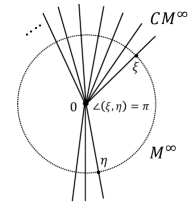
Figure 1: The boundary of hyperbolic space

Example 2.15.

Suppose that $M$ is a hyperbolic space. For distinct $\xi,\eta\in M^{\infty}$ there is a geodesic line $c:{\mathbb{R}}\to M$ such that $c(\infty)=\xi$ and $c(-\infty)=\eta$. This means that $\angle(\xi,\eta)=\pi$ for every distinct $\xi,\eta\in M^{\infty}$. Therefore, the boundary $M^{\infty}$ is a discrete topological space. See [11, II.9.6 (ii)]. The cone $CM^{\infty}$ is a star obtained from infinitely many half-lines ${\mathbb{R}}_{+}$, each associated with $\xi\in M^{\infty}$, by identifying the origin of all ${\mathbb{R}}_{+}$. See Figure 1. This can be seen from the distance formula (2.6) as $d^{\infty}(r\xi,s\eta)=r+s$ if $\xi\neq\eta$ and $|r-s|$ if $\xi=\eta$.

Let $f:M\to{\mathbb{R}}$ be a smooth convex function.

Lemma 2.16.

• $f^{\infty}$ is lower semicontinuous in the standard topology [33, Lemma 2.11].

• $(p,q)\mapsto\langle p,q\rangle$ is upper semicontinuous in the standard topology.

Proof.

(1). Take an arbitrary $x\in M$, and identify $CM^{\infty}$ with $T_{x}$ (by $v\mapsto\exp_{x}v\infty$). Let $f_{t}(p):=(f(\exp_{x}(pt))-f(x))/t$ for $p\in T_{x}$, which is monotone nondecreasing in $t$ and continuous on $T_{x}$ (in the standard topology). Therefore $f^{\infty}(p)=\sup_{t\geq 0}f_{t}(p)$. It is well-known that the supremum of continuous functions $f_{t}$ is lower semicontinuous.

(2). It is known [11, II.9.5] that $(\xi,\eta)\mapsto\angle(\xi,\eta)$ is lower semicontinuous. Then $(p,q)\mapsto\langle p,q\rangle$ is upper semicontinuous, since $p\mapsto d^{\infty}(0,p)=\|p\|_{x}$ is continuous in the standard topology and cosine is a decreasing function. ∎

As in the Euclidean case, a minimizer of $f$ is characterized by the gradient. The gradient $\nabla f(x)\in T_{x}$ of $f$ at $x$ is defined via

$$\langle\nabla f(x),v\rangle_{x}=df(x)(v)=\lim_{t\to 0}\{f(\exp_{x}tv)-f(x)\}/t\quad(v\in T_{x}),$$

where $df(x):T_{x}\to{\mathbb{R}}$ is the differential of $f$ at $x$. It is easy to see:

Lemma 2.17 (see [9, Corollary 11.22]).

$x\in M$ is a minimizer of $f$ if and only if $\nabla f(x)=0$.

In Euclidean case $M={\mathbb{R}}^{n}$, $x$ is a minimizer of $x\mapsto f(x)-\langle p,x\rangle$ if and only if $\nabla f(x)=p$. To extend it, we consider the gradient of Busemann functions. Note that Busemann functions are continuously differentiable; see [17, 1.10.2 (1)]. As in the previous subsection, we fix $x_{0}\in M$ and identify $CM^{\infty}$ with the space of Busemann functions for rays issuing from $x_{0}$.

Lemma 2.18 (see [17, 1.10.2 (2)]).

For $x\in M$ and $p\in CM^{\infty}$, it holds $\nabla b_{p}(x)=-u$ for $u\in T_{x}$ with $p=\exp_{x}\infty u$.

The asymptotic gradient $\nabla^{\infty}f(x)$ for $x\in M$ is defined as the asymptotic class of the ray $t\mapsto\exp_{x}t\nabla f(x)$, that is,

$$\nabla^{\infty}f(x):=\exp_{x}\infty\nabla f(x).$$

Notice that $\|\nabla^{\infty}f(x)\|=d^{\infty}(0,\nabla^{\infty}f(x))$ is the speed of $t\mapsto\exp_{x}t\nabla f(x)$. Therefore we have

$$\|\nabla^{\infty}f(x)\|=\|\nabla f(x)\|_{x}.$$ (2.19)

Then we have the following analogue of the one in Euclidean convex analysis.

Lemma 2.19.

For $p\in CM^{\infty}$, the following conditions are equivalent:

• $x$ is a minimizer of $f+b_{p}$ over $M$.

• $\nabla^{\infty}f(x)=p$.

• $f(x)+f^{*}(p)=-b_{p}(x)$

Proof.

(i) $\Leftrightarrow$ $\nabla(f+b_{p})(x)=0$ $\Leftrightarrow$ $\nabla f(x)=u$ for $p=\exp_{x}u\infty$ $\Leftrightarrow$ (ii). (i) $\Leftrightarrow$ (iii) is obvious from the definition (2.16) of conjugate $f^{*}$. ∎

As in the Euclidean case, the conjugate of a (smooth) convex function recovers the original function via the inverse transformation.

Lemma 2.20.

$f(x)=\sup_{p\in CM^{\infty}}-b_{p}(x)-f^{*}(p)\quad(x\in M).$

Proof.

By definition, $f^{*}(p)\geq-b_{p}(x)-f(x)$ for every $x\in M$ and $p\in CM^{\infty}$. Therefore $f(x)\geq\sup_{p\in CM^{\infty}}-b_{p}(x)-f^{*}(p)$. For $p=\nabla^{\infty}f(x)$, the equality is attained by Lemma 2.19. ∎

This gives rise to an interesting question of characterizing the class of functions $g$ on $CM^{\infty}$ for which $g^{*}(x):=\sup_{p\in CM^{\infty}}-b_{p}(x)-g(p)$ is convex on $M$. However this is beyond the theme of this paper, and we leave it for future research.

For a set $R\subseteq CM^{\infty}$, let $\mathop{\rm int}R$ denote the interior of $R$ in the $d^{\infty}$-topology.

Lemma 2.21.

Let $h:CM^{\infty}\to{\mathbb{R}}\cup\{\infty\}$ be a positively homogeneous function. Suppose that $h$ is lower semicontinuous in the standard topology. Then it holds

$$\mathop{\rm int}B(h)=\{p\in CM^{\infty}\mid\langle\xi,p\rangle<h(\xi)\ (\xi\in M^{\infty}\subseteq CM^{\infty})\}.$$ (2.20)

Proof.

Let $p\in B(h)$. Suppose that $\langle\xi,p\rangle=h(\xi)$ for some $\xi\in M^{\infty}$. Then, for arbitrary $\epsilon>0$, $\langle\xi,p+\epsilon\xi\rangle\geq\langle\xi,p\rangle+\epsilon\|\xi\|^{2}>h(\xi)$ (Lemma 2.3). This means $p+\epsilon\xi\not\in B(h)$. Since $\langle,\rangle$ is continuous (Lemma 2.3), $p$ is never an interior point of $B(h)$.

Suppose that $\langle\xi,p\rangle<h(\xi)$ for all $\xi\in M^{\infty}$. For $q\in CM^{\infty}$, let $\Delta(q):=\inf_{\xi\in M^{\infty}}h(\xi)-\langle\xi,q\rangle$. Since $M^{\infty}$ is compact and $\xi\mapsto h(\xi)-\langle\xi,q\rangle$ is lower semicontinuous in the standard topology (Lemma 2.16 (2)), the infimum is always attained. Let $\epsilon:=\Delta(p)>0$. Since $(q,\xi)\mapsto h(\xi)-\langle\xi,q\rangle$ is lower semicontinuous, for each $\xi\in M^{\infty}$ there is an open neighborhood $U_{\xi}\times V_{\xi}$ of $(p,\xi)$ (in the standard topology) such that for each $(q,\eta)\in U_{\xi}\times V_{\xi}$ we have $h(\eta)-\langle\eta,q\rangle\geq h(\xi)-\langle\xi,p\rangle-\epsilon\geq\Delta(p)-\epsilon=0$. Since $M^{\infty}$ is compact, there are $\xi_{1},\xi_{2},\ldots,\xi_{m}$ with $M^{\infty}=\bigcup_{i=1}^{m}V_{\xi_{i}}$. Let $U:=\bigcap_{i=1}^{m}U_{\xi_{i}}$, which is an open neighborhood of $p$ (in the standard topology). For any $q\in U$, $\Delta(q)=h(\xi^{\prime})-\langle\xi^{\prime},q\rangle$ for some $\xi^{\prime}$. Since $\xi^{\prime}$ belongs to $V_{\xi_{i}}$ for some $i$, it holds $\Delta(q)=h(\xi^{\prime})-\langle\xi^{\prime},q\rangle\geq 0$. Hence, we have $p\in U\subseteq B(h)$. Since the identify map on $CM^{\infty}$ from the $d^{\infty}$-topology to the standard topology is continuous, $U$ is an open neighborhood of $p$ in $d^{\infty}$-topology. ∎

As the proof shows, the RHS of (2.20) is the interior of $B(h)$ also in the standard topology, although $B(h)$ may not be closed in this topology.

We apply this lemma to the recession function $f^{\infty}$ and the associated subset $B(f^{\infty})$.

Proposition 2.22.

For $p\in\mathop{\rm int}B(f^{\infty})$, there is a minimizer of $f+b_{p}$. In particular, any point in $B(f^{\infty})\setminus\mathop{\rm dom}f^{*}$ belongs to the boundary of $B(f^{\infty})$.

See [31, Lemma 3.2 (iv)] for a related argument.

Proof.

Since $\xi\mapsto f^{\infty}(\xi)-\langle\xi,p\rangle$ is lower semicontinuous on compact set $M^{\infty}$ in the standard topology, the minimum value $\alpha>0$ exists. Let $\alpha^{\prime}\in(0,\alpha)$ and let $g:=f+b_{p}$. Fix an arbitrary $x\in M$. Then, for every $\xi\in M^{\infty}$ there is $t_{\xi}\in{\mathbb{R}}_{+}$ such that $g(\exp_{x}t\xi)-g(x)>\alpha^{\prime}t$ for all $t\geq t_{\xi}$. Define $h:M^{\infty}\to{\mathbb{R}}_{+}$ by

$$h(\xi):=\inf\{t\geq 0\mid g(\exp_{x}t\xi)-g(x)>\alpha^{\prime}t\}\quad(\xi\in M^{\infty}).$$

Then $h$ is upper semicontinuous, since the epigraph $\{(\xi,t)\in M^{\infty}\times{\mathbb{R}}\mid t\leq h(\xi)\}$ is the closed set $\{(\xi,t)\in M^{\infty}\times{\mathbb{R}}_{+}\mid g(\exp_{x}t\xi)-g(x)\leq\alpha^{\prime}t\}\cup\{(\xi,t)\in M^{\infty}\times{\mathbb{R}}\mid t\leq 0\}$. Since $M^{\infty}$ is compact, the maximum $t^{*}$ of $h$ over $M^{\infty}$ exists. Then, for every $\xi\in M^{\infty}$, we have $g(\exp_{x}t\xi)-g(x)\geq\alpha^{\prime}t$ for all $t\geq t^{*}$. This means that the level set $\{y\in M\mid g(y)\leq g(x)+\alpha^{\prime}t^{*}\}$ belongs to the metric ball at center $x$ with radius $t^{*}$, which is compact by Hopf-Rinow theorem (see [42, III.1]). A minimizer of $g$ exists in this set. ∎

Thus we have

$$\mathop{\rm int}B(f^{\infty})\subseteq\nabla^{\infty}f(M)\subseteq\mathop{\rm dom}f^{*}\subseteq B(f^{\infty}).$$ (2.21)

We next provide a characterization of $B(f^{\infty})$, which sharpens the following important result by Kapovich, Leeb, and Millson [31].

Theorem 2.23 ([31, Lemma 3.4]).

If $f^{\infty}(u)\geq 0$ for all $u\in M^{\infty}$, i.e., $0\in B(f^{\infty})$, then $\inf_{x\in M}\|\nabla f(x)\|_{x}=0$.

An outline of the proof is as follows: If $\inf_{x\in M}\|\nabla f(x)\|_{x}>0$, then a trajectory of the normalized gradient flow of $f$ goes to $u\in M^{\infty}$ with $f^{\infty}(u)<0$; See also [46, section 5.4].

We now obtain an analogue of the equivalence between (a) and (c) in the introduction.

Theorem 2.24.

For $p\in CM^{\infty}$, the following are equivalent:

• $\inf_{x\in M}\|\nabla(f+b_{p})(x)\|_{x}=0$.

• $p\in B(f^{\infty})$.

Proof.

(c) $\Rightarrow$ (a) follows from applying the above theorem to $f+b_{p}$. We verify (a) $\Rightarrow$ (c). Let $g:=f+b_{p}$. For arbitrary $\epsilon>0$, there is $x\in M$ such that $\|\nabla g(x)\|_{x}<\epsilon$. Consider $u\in M^{\infty}$ and the geodesic ray $t\mapsto\exp_{x}vt$ with $\exp_{x}v\infty=u$. Then $\lim_{t\to 0}(g(\exp_{x}vt)-g(x))/t=\langle\nabla g(x),v\rangle_{x}=\|\nabla g(x)\|_{x}\cos\theta>-\epsilon$, where $\theta$ is the angle between $\nabla g(x)$ and $v$ in $T_{x}$. Since $(g(\exp_{x}vt)-g(x))/t$ is monotone nondecreasing, by $t\to\infty$ we have $g^{\infty}(u)=f^{\infty}(u)-\langle u,p\rangle>-\epsilon$. Thus, for every $\epsilon>0$ and $u\in M^{\infty}$, it holds $\langle u,p\rangle<f^{\infty}(u)+\epsilon$. This implies $p\in B(f^{\infty})$. ∎

The condition (a) $\inf_{x\in M}\|\nabla(f+b_{p})(x)\|_{x}=0$ may be viewed as a correspondent of $\inf_{x\in{\mathbb{R}}^{n}}\|\nabla f(x)-p\|=0$ of the Euclidean case. If $\nabla^{\infty}f(x_{i})$ $(i=1,2,\ldots)$ converges to $p\in CM^{\infty}$ in the $d^{\infty}$-topology, then (a) holds. Indeed, by Lemma 2.18 and (2.19) it holds

$$\|\nabla(f+b_{p})(x)\|_{x}^{2} = \|\nabla f(x)\|_{x}^{2}+\|u\|_{x}^{2}-2\|\nabla f(x)\|_{x}\|u\|_{x}\cos\theta_{x}$$

$$\leq \|\nabla^{\infty}f(x)\|^{2}+\|p\|^{2}-2\|\nabla^{\infty}f(x)\|\|p\|\cos\theta$$

$$= d^{\infty}(\nabla^{\infty}f(x),p)^{2},$$

where $u:=-\nabla b_{p}(x)$, $\theta_{x}$ is the angle between $\nabla f(x)$ and $u$ in $T_{x}$, and $\theta:=\angle(\nabla^{\infty}f(x),p)$ ($\geq\theta_{x}$ by definition (2.5)). However, the converse is not true. Also (a) does not mean the convergence in the standard topology.

2.3 Symmetric spaces of nonpositive curvature

Here we consider symmetric spaces of nonpositive curvature, which constitute a fundamental class of Hadamard manifolds. Our argument basically consults [17, Chapters 2 and 3]. In a Hadamard manifold $M$ and a point $x$, the geodesic symmetry $\sigma_{x}:M\to M$ at $x$ is defined by $\sigma_{x}(\exp_{x}(v))=\exp_{x}(-v)$ for $v\in T_{x}$. A symmetric space of nonpositive curvature is a Hadamard manifold $M$ such that for every $x\in M$ the geodesic symmetry $\sigma_{x}$ is an isometry on $M$. Via the de Rham decomposition theorem (see [42, III.6]), $M$ is (uniquely) decomposed as Riemannian product $M=M_{0}\times N$, where $M_{0}$ is isometric to Euclidean space ${\mathbb{R}}^{k}$ $(k\geq 0)$ (called the Euclidean de Rham factor of $M$) and a symmetric space $N$ of noncompact type, i.e., it is given by $N=G/K$ for a (real) semisimple Lie group $G$ and its maximal compact subgroup $K$. Then $N$ has a trivial Euclidean de Rham factor, and its Riemannian structure is given by a $G$-invariant metric. We will see more concrete constructions in Sections 2.4 and 3.2.

Let $M$ be a symmetric space of nonpositive curvature, and let $x_{0}\in M$. A $k$-dimensional flat is a submanifold of $M$ isometric to ${\mathbb{R}}^{k}$. A maximal flat is a flat that is not contained in another flat of a larger dimension. It is a basic fact that all maximal flats have the same dimension $d$, which is called the rank of $M$. By a geodesic line we mean a map $l:{\mathbb{R}}\to M$ with $d(l(s),l(t))=|s-t|$ for $s,t\in{\mathbb{R}}$, which is just a $1$-dimensional flat. A geodesic line is called regular if it is contained by a unique maximal flat. Let $x\in M$ and let $F$ be a maximal flat containing $x$. A Weyl chamber at tip $x$ is the closure of a connected component of the set of points $y\in F\setminus\{x\}$ such that the unique geodesic line containing $x,y$ is regular. When $F$ is viewed as ${\mathbb{R}}^{d}$ with origin $x$, Weyl chambers are polyhedral cones. They have the same shape, since the group $G$ acts transitively on them.

We next explain the building structure of the boundary $M^{\infty}$ and its cone $CM^{\infty}$; [7, Appendix 5] is a useful reference. It is clear (from Example 2.4) that the boundary $F^{\infty}$ of a maximal flat $F$ is isometric to sphere $S^{d-1}$. The boundary $C^{\infty}$ of a Weyl chamber $C$ (at some tip) is called an (asymptotic) Weyl chamber. For two Weyl chambers $C,D$ (at possibly different tips), the asymptotic ones $C^{\infty},D^{\infty}$ are the same or have disjoint interiors. Then, the set of all Weyl chambers and their faces give rise to a cell-complex structure on $M^{\infty}$, where each cell is isometric to a polyhedral cell in a sphere (the intersection of a sphere and a polyhedral cone). This structure is an $M_{1}$-polyhedral complex in the sense of [11, Chapter I.7], and forms a spherical building, where an apartment is precisely the subcomplex formed by the boundary of a maximal flat. Although Weyl chambers here may not be simplices, one can subdivide them to obtain a simplicial complex ${\cal C}$ so that each apartment is a spherical Coxeter complex. Then the apartments are glued nicely. That is, they satisfy, as an abstract simplicial complex, the axiom of building:

• Any two simplices in ${\cal C}$ are contained in a common apartment.

• For two apartments $A,A^{\prime}$ including simplices $C,C^{\prime}$, there is an isomorphism $A\to A^{\prime}$ fixing $C,C^{\prime}$ pointwise.

See e.g., [1] and [11, II.10. Appendix] for (formal) theory of building. By considering the Euclidean cone, $CM^{\infty}$ has the structure of a Euclidean building. A maximal cone is also called a Weyl chamber. Apartments are the subcomplexes induced by $CF^{\infty}$ for all maximal flats $F$. We simply call $CF^{\infty}$ an apartment. Each apartment is a convex subspace of $CM^{\infty}$ isometric to ${\mathbb{R}}^{d}$. We can identify an apartment $E\subseteq CM^{\infty}$ with ${\mathbb{R}}^{d}$ so that the origins coincide. In this identification, $\langle,\rangle$ in $E$ is precisely the Euclidean inner product of ${\mathbb{R}}^{d}$.

Suppose that $M={\mathbb{R}}^{k}\times N$, where $N$ is a symmetric space $G/K$ of noncompact type. Then $CM^{\infty}={\mathbb{R}}^{k}\times CN^{\infty}$. The structure of building $CM^{\infty}$ is determined by $CN^{\infty}$. We can suppose (as in [17]) that $G$ is the identity component of the group of isometries of $N$, where $G$ acts isometrically on $M={\mathbb{R}}^{k}\times N$ by ${\mathbb{R}}^{k}\times N\ni(x^{\prime},x)\mapsto(x^{\prime},gx)$. Since any isometry on $M$ induces an isometry on $M^{\infty}$, the group $G$ acts isometrically on $M^{\infty}$ and on $CM^{\infty}$ by $gp=\|p\|g(p/\|p\|)$. Also $G$ acts on the set of Weyl chambers and their faces. The facial incidence structure of the building $M^{\infty}$ is described by the inclusion relation of all parabolic subgroups of $G$. Here a parabolic subgroup is the subgroup consisting of $g\in G$ with $g\xi=\xi$ for some $\xi\in N^{\infty}$, which is denoted by $G_{\xi}$. If $\xi,\xi^{\prime}$ belong to the relative interior of the same face of a Weyl chamber, then $G_{\xi}=G_{\xi^{\prime}}$. Therefore, minimal parabolic subgroups correspond to Weyl chambers. Fix a Weyl chamber $C_{0}$, and regard it as a polyhedral cone in ${\mathbb{R}}^{d}$. Let $P$ be the minimal parabolic subgroup for $C_{0}$. The set of Weyl chambers is identified with the flag variety $G/P$. If $p\in CM^{\infty}$ belongs to a Weyl chamber corresponding to ${\cal F}\in G/P$ and the orbit of $p\in CM^{\infty}$ by $G$-action meets a (unique) point $\lambda$ in $C_{0}\subseteq{\mathbb{R}}^{d}$, then we denote $p$ by

$$p=\lambda\cdot{\cal F}.$$ (2.22)

This notation designates the coordinate $\lambda$ of $p$ in the Weyl chamber indexed by ${\cal F}$.

Two geodesic lines $c,c^{\prime}:{\mathbb{R}}\to M$ are said to be parallel if $d(c(t),c^{\prime}(t))$ $(t\in{\mathbb{R}})$ is bounded above. For a geodesic line $c$, let $F(c)$ denote the union of all geodesic lines parallel to $c$. It is known that $F(c)$ is a totally geodesic submanifold of $M$. If $c$ is regular, $F(c)$ is a maximal flat.

For $\xi\in N^{\infty}$, the horospherical subgroup $N_{\xi}$ of $G_{\xi}$ consists of $n\in G$ such that $\lim_{t\to\infty}d(n(c(t)),c(t))=0$, where $c$ is the geodesic ray with $c(\infty)=\xi$ and $c(0)=x_{0}$ (independent of $x_{0}$). Then $N_{\xi}$ keeps the Busemann function $b_{\xi}$ as $b_{\xi}(nx)=b_{\xi}(x)$, since $|b_{\xi}(nx)-b_{\xi}(x)|=\lim_{t\to\infty}|d(x,n^{-1}c(t))-d(x,c(t))|\leq\lim_{t\to\infty}d(c(t),n^{-1}c(t))=0$. The generalized Iwasawa decomposition [17, 2.17.5 (5)] implies that $M$ is diffeomorphic to $N_{\xi}\times F(c)$ by $(n,y)\mapsto n(y)$.

In this setting, let us start our convex analysis on $M$. Let $f:M\to{\mathbb{R}}$ be a smooth convex function. For a maximal flat $F$, let $f_{F}:F\to{\mathbb{R}}$ denote the restriction of $f$ to $F$. The asymptotic Legendre-Fenchel conjugate ${f_{F}}^{*}:CF^{\infty}\to{\mathbb{R}}\cup\{\infty\}$ is defined by ${f_{F}}^{*}(p):=\sup_{x\in F}-b_{p}(x)-f(x)$, where $x_{0}$ may be outside of $F$. By $p\in CF^{\infty}$ and Example 2.7, $b_{p}$ is an affine function on $F$. Therefore, ${f_{F}}^{*}$ is viewed as the ordinary Legendre-Fenchel conjugate (up to an additive constant) under identification $CF^{\infty}={\mathbb{R}}^{d}$. Hence we have:

Lemma 2.25.

For any maximal flat $F$, ${f_{F}}^{*}$ is a convex function on $CF^{\infty}$.

Still, $f^{*}$ may be nonconvex but “partially” convex in the following sense:

Proposition 2.26.

For a Weyl chamber $C\subseteq CM^{\infty}$, it holds

$$f^{*}(p)=\sup_{F}{f_{F}}^{*}(p)\quad(p\in C),$$ (2.23)

where $\sup$ is taken over all maximal flats $F$ with $CF^{\infty}\supseteq C$. In particular, $f^{*}$ is a convex function on $C$, and $C\cap\mathop{\rm dom}f^{*}$ is a convex set contained by a convex set $\bigcap_{F}C\cap\mathop{\rm dom}{f_{F}}^{*}$:

$$C\cap\mathop{\rm dom}f^{*}\subseteq\bigcap_{F}C\cap\mathop{\rm dom}{f_{F}}^{*}.$$ (2.24)

Note that $\subseteq$ may be strict since $f^{*}(p)=\sup_{F}{f_{F}}^{*}(p)$ may be $\infty$ even if ${f_{F}}^{*}(p)<\infty$ for every $F$.

Proof.

Consider the Iwasawa decomposition $M=N\times F_{0}$, where $F_{0}$ is a maximum flat containing $C$ at infinity and $N$ is the holospherical subgroup for $C$. Then $NF_{0}$ ranges over all maximal flats containing $C$ at infinity. Thus $M$ is the (disjoint) union of all maximal flats $F$ such that $F^{\infty}\supseteq C\ni p$. Then we have $f^{*}(p)=\sup_{F}\sup_{x\in F}-b_{p}(x)-f(x)=\sup_{F}{f_{F}}^{*}(p)$. ∎

Next, we consider the recession function $f^{\infty}$ and the associated subset $B(f^{\infty})$. For each apartment $E$, we also consider

$$B_{E}(f^{\infty}):=\{p\in E\mid\langle u,p\rangle\leq f^{\infty}(u)\ (u\in E)\}.$$ (2.25)

Proposition 2.27.

For a Weyl chamber $C\subseteq E$, it holds

$$C\cap B(f^{\infty})=\bigcap_{F}C\cap B_{CF^{\infty}}(f^{\infty})=\bigcap_{F}C\cap\overline{\mathop{\rm dom}{f_{F}}^{*}}.$$ (2.26)

where $\bigcap$ is taken over all maximal flats $F$ with $CF^{\infty}\supseteq C$. In particular, $C\cap B(f^{\infty})$ is a convex set in $C$.

Proof.

Since $CM^{\infty}$ is the union of all apartments $E$ containing any fixed Weyl chamber $C$, we have the first equality. When $E$ is viewed as Euclidean space ${\mathbb{R}}^{n}$, then $C$ is a convex cone, $\langle u,p\rangle\leq f^{\infty}(u)$ is a linear inequality, and therefore $C\cap B_{E}(f^{\infty})$ is convex. Necessarily the intersection $\bigcap_{E}C\cap B_{E}(f^{\infty})$ is convex. By Lemma 2.16, the restriction of $f^{\infty}$ to Euclidean space $E$ is lower semicontinuous and positively homogeneous convex, and must be the support function of $\mathop{\rm dom}{f_{F}}^{*}$. Hence we have $\overline{\mathop{\rm dom}{f_{F}}^{*}}=B_{E}({f}^{\infty})$, and the second equality. ∎

In the view of (2.24) and (2.26), the closure $\overline{\mathop{\rm dom}f^{*}}$ seems very close to $B(f^{\infty})$, although we do not know whether they really differ. Under non-degeneracy assumptions, three spaces $\nabla^{\infty}f(M)$, $\overline{\mathop{\rm dom}f^{*}}$, and $B(f^{\infty})$ are equal, as in Euclidean case.

Proposition 2.28.

For a Weyl chamber $C$, if $C\cap B(f^{\infty})$ has nonempty interior, then $C\cap\overline{\nabla^{\infty}f(M)}=C\cap\overline{\mathop{\rm dom}f^{*}}=C\cap B(f^{\infty})$.

Proof.

By (2.21), it holds

$$C\cap\mathop{\rm int}B(f^{\infty})\subseteq C\cap\overline{\nabla^{\infty}f(M)}\subseteq C\cap\overline{\mathop{\rm dom}f^{*}}\subseteq C\cap B(f^{\infty}).$$ (2.27)

In Euclidean space, for any closed convex set $D$ having nonempty interior, it holds $\overline{\mathop{\rm int}D}=D$. This can be applied to $C\cap B(f^{\infty})$, which is viewed as a Euclidean convex set. From $C\cap B(f^{\infty})=\overline{\mathop{\rm int}(C\cap B(f^{\infty}))}\subseteq\overline{C\cap\mathop{\rm int}B(f^{\infty})}\subseteq C\cap B(f^{\infty})$, by taking the closure in (2.27), we have the claim. ∎

Proposition 2.29.

Suppose that $f$ is strictly convex. Then the gradient map $x\mapsto\nabla^{\infty}f(x)$ is a bijection from $M$ to $\mathop{\rm int}B(f^{\infty})$. For a Weyl chamber $C$, if $C\cap\nabla^{\infty}f(M)\neq\emptyset$, then $C\cap\overline{\nabla^{\infty}f(M)}=C\cap\overline{\mathop{\rm dom}f^{*}}=C\cap B(f^{\infty})$.

Proof.

We first verify $\nabla^{\infty}f:M\to CM^{\infty}$ is injective. Indeed, if $\nabla^{\infty}f(x)=\nabla^{\infty}f(y)=p$, then $x$ and $y$ are minimizers of $f+b_{p}$, and it must hold $x=y$ by strict convexity of $f+b_{p}$. For surjectivity, from Proposition 2.22 it suffices to show that $\nabla^{\infty}f(x)$ for any $x\in M$ belongs to $\mathop{\rm int}B(f^{\infty})$. We utilize the following property, where $C$ is a Weyl chamber.

$$b_{p}+b_{q}=b_{p+q}\quad(p,q\in C).$$ (2.28)

Indeed, consider a maximal flat $F$ containing $x_{0}$ and $C$ at infinity, and consider horospherical subgroup $N$ of $C$ and Iwasawa decomposition $M=N\times F$. If $x=n(y)$ for $n\in N$ and $y\in F$, then $b_{p}(x)+b_{q}(x)=b_{p}(y)+b_{q}(y)=-\langle p,y-x_{0}\rangle-\langle q,y-x_{0}\rangle=-\langle p+q,y-x_{0}\rangle=b_{p+q}(y)=b_{p+q}(x)$, where $p+q\in C$ and $F$ is viewed as ${\mathbb{R}}^{d}$ (see Example 2.7).

Let $p:=\nabla^{\infty}f(x)$ for $x\in M$. Suppose that $0\neq p=\|p\|\xi$ for $\xi\in M^{\infty}$. Consider sufficiently small $\epsilon>0$. Let $B_{\epsilon}$ be the set of all points $q$ represented as $q=(\|p\|-t)\xi+2t\eta$, where $t\leq\epsilon$ and $\xi,\eta\in CM^{\infty}$ belong to the same Weyl chamber. Then $B_{\epsilon}$ contains $p$ in its interior.

We show that $B_{\epsilon}\subseteq\nabla^{\infty}f(M)$ for small $\epsilon>0$. By strict convexity of $f$, $x$ is a unique minimizer of $f+b_{p}$. Let $\alpha>0$ be the minimum of $(f+b_{p})(\exp_{x}v)-(f+b_{p})(x)$ over all $v\in T_{x}$ with $\|v\|_{x}=1$, which exists by compactness. For $q=(\|p\|-t)\xi+2t\eta\in B_{\epsilon}$, it holds $f+b_{q}=f+b_{p}-tb_{\xi}+2tb_{\eta}$ by (2.28). Here the additional term $-tb_{\xi}+2tb_{\eta}$ is $3\epsilon$-Lipschitz (Lemma 2.5). For $3\epsilon\leq\alpha$, a minimizer of $f+b_{q}$ exists in the unit ball around $x$. Thus $q\in\nabla^{\infty}f(M)$, as required. The proof of the case $p=0$ is similar; omit $-t\xi$ above.

If $\nabla^{\infty}f(M)\cap C\neq 0$, then $\nabla^{\infty}f(M)\cap C$ has nonempty interior, and Proposition 2.28 is applicable to obtain the latter statement. ∎

Note that there is a possibility that $C\cap\nabla^{\infty}f(M)$ is empty but $C\cap B(f^{\infty})$ is nonempty and has no interior. Further refined study on such a degenerate situation is left for future research.

Via the inverse of $x\mapsto\nabla^{\infty}f(x)$, the symmetric space $M$ is coordinated by the asymptotic gradient space $\nabla^{\infty}f(M)$. This can be viewed as a generalization of the dual coordinate of dually-flat manifolds in information geometry [3]. It is an interesting research direction to develop an information-geometrical theory based on this idea.

In the case of $\mathop{\rm dom}f^{*}=B(f)$ which we will face in Section 3, the boundedness of $\inf_{x\in M}(f+b_{p})(x)$ is verified by convex optimization on Euclidean building $CM^{\infty}$:

$$\mbox{inf.}\quad f^{\infty}(u)-\langle u,p\rangle\quad\mbox{s.t.}\quad u\in U,$$ (2.29)

where $U\subseteq CM^{\infty}$ is any convex neighborhood of the origin, such as a ball.

2.4 Symmetric space $P_{n}=GL(n,{\mathbb{C}})/U(n)$

Here we consider the symmetric space $P_{n}=GL(n,{\mathbb{C}})/U(n)$ of positive definite Hermitian $n\times n$ matrices, and present concrete descriptions and specializations of several concepts introduced above. Arguments regarding the PSD-cone as a symmetric space are found in [11, Chapter II.10] and [17, 2.2.13], where they consider $GL(n,{\mathbb{R}})/O(n)$ or $SL(n,{\mathbb{R}})/SO(n)$ but the arguments are analogous.

When regarding $P_{n}$ as a Riemannian manifold, the tangent space $T_{x}$ at $x\in P_{n}$ is identified with the space $S_{n}$ of $n\times n$ Hermitian matrices and the inner product is given by $\langle H,H^{\prime}\rangle_{x}=\mathop{\rm tr}x^{-1}Hx^{-1}H^{\prime}$. The cotangent space $T_{x}^{\ast}$ is also identified with $S_{n}$ by $H(H^{\prime}):=\mathop{\rm tr}HH^{\prime}$ for $H,H^{\prime}\in S_{n}$. Let $d$ denote the corresponding distance function on $M$. The exponential map $\exp_{x}:T_{x}\to P_{n}$ at $x$ is given by $H\mapsto x^{1/2}e^{x^{-1/2}Hx^{-1/2}}x^{1/2}$. In particular, any constant-speed ray is written as $t\mapsto ge^{t\mathop{\rm diag}\lambda}g^{\dagger}$ for $\lambda\in{\mathbb{R}}^{n}$ and $g\in GL(n,{\mathbb{C}})$, where $\mathop{\rm diag}\lambda$ denotes the diagonal matrix with diagonal entries $\lambda_{1},\lambda_{2},\ldots,\lambda_{n}$ in order, and $(\cdot)^{\dagger}$ denotes the complex conjugate. By $(g,x)\mapsto gxg^{\dagger}$, $GL(n,{\mathbb{C}})$ acts isometrically and transitively on $P_{n}$. The isotropy group at $I$ is the group $U(n)$ of unitary matrices. So $P_{n}$ is a symmetric space $GL(n,{\mathbb{C}})/U(n)={\mathbb{R}}\times(SL(n,{\mathbb{C}})/SU(n))$, where the geodesic symmetry at $x\in P_{n}$ is given by $y\mapsto xy^{-1}x$. The identity matrix $I$ is naturally chosen as the base point $x_{0}$ of $P_{n}$.

Any maximal flat is the set of matrices of form

$$F(g):=\{ge^{\mathop{\rm diag}\lambda}g^{\dagger}\mid\lambda\in{\mathbb{R}}^{n}\}$$ (2.30)

for $g\in GL(n,{\mathbb{C}})$, where $\lambda\mapsto ge^{\mathop{\rm diag}\lambda}g^{\dagger}$ is an isometry from ${\mathbb{R}}^{n}$ to $F(g)$. From this, we see that a geodesic ray $t\mapsto ge^{t\mathop{\rm diag}\lambda}g^{\dagger}$ is regular if and only if all values $\lambda_{i}$ are different. A vector $\lambda\in{\mathbb{R}}^{n}$ is said to be arranged if $\lambda_{1}\geq\lambda_{2}\geq\cdots\geq\lambda_{n}$. The next lemma characterizes asymptotic classes of geodesic rays.

Lemma 2.30 (See [11, II.10.64]).

For arranged vectors $\lambda,\mu\in{\mathbb{R}}^{n}$ with $\|\lambda\|_{2}=\|\mu\|_{2}=1$ and $g,h\in GL(n,{\mathbb{C}})$, two geodesic rays $t\mapsto ge^{t\mathop{\rm diag}\lambda}g^{\dagger}$ and $t\mapsto he^{t\mathop{\rm diag}\mu}h^{\dagger}$ are asymptotic if and only if $\lambda=\mu$ and $(h^{-1}g)_{ij}=0$ for all $i\geq j$ with $\lambda_{i}<\lambda_{j}$.

Proof.

Let $b(t):=e^{-t\mathop{\rm diag}\mu/2}h^{-1}ge^{t\mathop{\rm diag}\lambda/2}$, where $b(t)_{ij}=e^{-t(\mu_{i}-\lambda_{j})/2}(h^{-1}g)_{ij}$. Then we have $d(ge^{t\mathop{\rm diag}\lambda}g^{\dagger},he^{t\mathop{\rm diag}\mu}h^{\dagger})=d(b(t)b(t)^{\dagger},I)$. Consider the smallest $i$ with $\lambda_{i}\neq\mu_{i}$ if it exists. Say $\lambda_{i}<\mu_{i}$. Then $\lim_{t\to\infty}b(t)$ has a zero block of $i$ rows and $n-i+1$ columns, and is singular (and/or has a $\infty$ entry). Necessarily $d(b(t)b(t)^{\dagger},I)\to\infty$. If $\lambda=\mu$ and $(h^{-1}g)_{ij}\neq 0$ for some $i\geq j$ with $\lambda_{i}<\lambda_{j}$, then $(b(t)b(t)^{\dagger})_{ii}\to\infty$, implying $d(b(t)b(t)^{\dagger},I)\to\infty$. Conversely, suppose that the condition is satisfied. Then $b(t)$ converges to a constant matrix. This means that $d(b(t)b(t)^{\dagger},I)$ is bounded, and the two rays are asymptotic. ∎

Thus, the minimal parabolic subgroup for Weyl chamber $C_{0}:=\{e^{\infty\mathop{\rm diag}\lambda}\mid\lambda:\mbox{arranged}\}$ is the group $B$ of upper triangular matrices. Then $GL(n,{\mathbb{C}})/B$ is viewed as the space of complete flags $U_{1}\subset U_{2}\subset\cdots\subset U_{n}={\mathbb{C}}^{n}$ of vector subspaces $U_{i}$ of ${\mathbb{C}}^{n}$. As an abstract simplicial complex, the building $CP_{n}^{\infty}$ is the order complex of the lattice of all (nonzero) vector subspaces of ${\mathbb{C}}^{n}$. As consistent with (2.22), any point $p$ in $CP^{\infty}_{n}$ is represented as $p=\lambda\cdot{\cal U}$ for an arranged vector $\lambda$ and complete flag ${\cal U}$. Specifically, if $p$ is written as $p=ge^{\infty\lambda}g^{\dagger}$ for an arranged vector $\lambda$ and $g\in GL(n,{\mathbb{C}})$, then ${\cal U}$ is the complete flag consisting of vector subspaces spanned by the first $i$ columns of $g$ for $i=1,2,\ldots,n$. The $i$-th vector subspaces of complete flags ${\cal U}$ and ${\cal V}$ are denoted by $U_{i}$ and $V_{i}$, respectively. Lemma 2.30 rephrases as: $\lambda\cdot{\cal U}=\mu\cdot{\cal V}$ if and only if $\lambda=\mu$ and $U_{i}=V_{i}$ for each $i\in[n-1]$ with $\lambda_{i}>\lambda_{i+1}$. By associating $\lambda\cdot{\cal U}$ with formal sum $\sum_{i=1}^{n}(\lambda_{i}-\lambda_{i+1})U_{i}$ with $\lambda_{n+1}:=0$, the boundary $CP^{\infty}_{n}$ is also identified with the set of all formal sums

$$p=\sum_{i}\alpha_{i}U_{i},$$ (2.31)

where vector subspaces $U_{i}$ form a (partial) flag and nonzero coefficients $\alpha_{i}\in{\mathbb{R}}$ are positive if $U_{i}\neq{\mathbb{C}}^{n}$. Note that this expression (2.31) is unique. In this way, any single vector subspace $X(=1X)$ is viewed as a point of $CP_{n}^{\infty}$.

A Weyl chamber $C\subseteq CP^{\infty}_{n}$ consists of $\lambda\cdot{\cal U}$ over all arranged vectors $\lambda$ for a (fixed) flag ${\cal U}$. The distance $d^{\infty}(p,q)$ of two points $\lambda\cdot{\cal U}$ and $\mu\cdot{\cal U}$ in the same chamber is given by $\|\lambda-\mu\|_{2}$. Accordingly, the distance of any two points in $CP^{\infty}_{n}$ is given by the length metric of the two points (the infimum of the length of a path connecting them). The whole space $CP^{\infty}_{n}$ is a polyhedral cone complex obtained by gluing these Euclidean polyhedral cones. An apartment $E(g):=F(g)^{\infty}=\{ge^{\infty\mathop{\rm diag}\lambda}g^{\dagger}\mid\lambda\in{\mathbb{R}}^{n}\}$ for $g\in GL(n,{\mathbb{C}})$ consists of all points of form $\lambda\cdot{\cal U}$ such that each subspace $U_{i}$ in flag ${\cal U}$ is spanned by column vectors of $g$. $GL(n,{\mathbb{C}})$ acts isometrically on $CP^{\infty}_{n}$ by $(g,\lambda\cdot{\cal U})\mapsto\lambda\cdot g{\cal U}$.

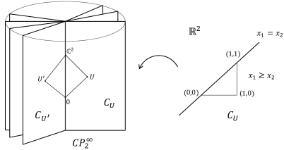
Figure 2: The boundary $CP_{2}^{\infty}$ of $P_{2}$

Example 2.31.

Consider the case of $n=2$. Any complete flag ${\cal U}$ is uniquely determined by its $1$-dimensional subspace $U=U_{1}$. The corresponding Weyl chamber is a form of $\{\lambda\cdot{\cal U}\mid\lambda\in{\mathbb{R}}^{2},\lambda_{1}\geq\lambda_{2}\}$, and is isometric to half-plane $\{x\in{\mathbb{R}}^{2}\mid x_{1}\geq x_{2}\}:=C_{U}\subseteq{\mathbb{R}}^{2}$. Then $CP_{2}^{\infty}$ is obtained by gluing $C_{U}$ for all $1$-dimensional subspaces $U$, along the line of $x_{1}=x_{2}$. Specifically, it is the disjoint union $\coprod_{U}C_{U}$ over all $1$-dimensional subspaces $U$ modulo the equivalence relation: $(U,x)\sim(U^{\prime},x^{\prime})$ if and only if $x_{1}=x_{2}=x_{1}^{\prime}=x_{2}^{\prime}$. Subspaces $U$ and ${\mathbb{C}}^{2}$ are the points of $CP_{2}^{\infty}$ that are the images of $(U,(1,0))$ and $(U,(1,1))$, respectively. See Figure 2. This shape of $CP_{2}^{\infty}$ can be directly seen from the expression $CP_{2}^{\infty}={\mathbb{R}}\times C(SL(2,{\mathbb{C}})/SU(2))^{\infty}$. Here $SL(2,{\mathbb{C}})/SU(2)$ is a $3$-dimensional hyperbolic space, and $C(SL(2,{\mathbb{C}})/SU(2))^{\infty}$ is an infinite star (Example 2.15).

In this setting, we present explicit descriptions of Busemann functions, asymptotic gradients, and inner product $\langle,\rangle$ on $CP_{n}^{\infty}$. For $g\in GL(n,{\mathbb{C}})$, let $[g]$ denote the image in $G/B$, which is the complete flag of vector subspaces spanned by the first $i$ columns of $g$ for $i=1,2,\ldots,n$. For a Hermitian matrix $H$ and subset $I\subseteq[n]:=\{1,2,\ldots,n\}$, let $H[I]$ denote the principal matrix of $H$ consisting of row/column indices in $I$, where $H[\emptyset]:=1$.

Lemma 2.32 (see [11, II.10.69]).

For $p=\lambda\cdot[u]\in CP_{n}^{\infty}$ with $u\in U(n)$, it holds

$$b_{p}(x) = -\sum_{i=1}^{n}\lambda_{i}\log\frac{\det(u^{\dagger}xu)[\{i,\ldots,n\}]}{\det(u^{\dagger}xu)[\{i+1,\ldots,n\}]},$$ (2.32)

$$\nabla b_{p}(x) = -ub\mathop{\rm diag}\lambda b^{\dagger}u^{\dagger},$$ (2.33)

where $u^{\dagger}x^{1/2}=bk$ for upper triangular matrix $b$ and unitary matrix $k$ (Gram–Schmidt orthonormalization).

Proof.

It suffices to consider $p\in P_{n}^{\infty}$. The geodesic ray $c$ issuing from $I$ with $c(\infty)=p$ is written as $c(t)=ue^{t\mathop{\rm diag}\lambda}u^{\dagger}$. Therefore, we have $b_{p}(x)=\lim_{t\to\infty}d(ue^{t\mathop{\rm diag}\lambda}u^{\dagger},x)-t=\lim_{t\to\infty}d(e^{t\mathop{\rm diag}\lambda},u^{\dagger}xu)-t$. Suppose that all $\lambda_{i}$ are different. Decompose $u^{\dagger}xu$ as $u^{\dagger}xu=n\mathop{\rm diag}rn^{\dagger}$, where $n$ is an upper triangular matrix having $1$ on each diagonal and $r\in{\mathbb{R}}^{n}$ is a positive vector with $r_{i}$ written as

$$r_{i}=\frac{\det(u^{\dagger}xu)[\{i,\ldots,n\}]}{\det(u^{\dagger}xu)[\{i+1,\ldots,n\}]}.$$ (2.34)

As in the proof of Lemma 2.30, it holds $\lim_{t\to\infty}d(n^{-1}e^{t\mathop{\rm diag}\lambda}n^{-\dagger},e^{t\mathop{\rm diag}\lambda})=0$, and we have $b_{p}(x)=\lim_{t\to\infty}d(e^{t\mathop{\rm diag}\lambda},\mathop{\rm diag}r)-t=\lim_{t\to\infty}\|t\mathop{\rm diag}\lambda-\log r\|_{2}-t=-\sum_{i=1}^{n}\lambda_{i}\log r_{i}$ (see Example 2.7), where $\log r\in{\mathbb{R}}^{n}$ is defined by $(\log r)_{i}:=\log r_{i}$. Then we obtain (2.32) from (2.34). If some of $\lambda_{i}$ are equal, we decompose $u^{\dagger}xu$ to $nyn^{\dagger}$, where $n$ is an upper triangular matrix satisfying $n_{ii}=1$ and $n_{ij}=n_{ji}=0$ if $\lambda_{i}=\lambda_{j}$ and $i\neq j$, and $y$ is a block diagonal matrix with $y_{ij}=y_{ji}=0$ if $\lambda_{i}\neq\lambda_{j}$. As above, it holds $b_{p}(x)=\lim_{t\to\infty}d(e^{t\mathop{\rm diag}\lambda},y)-t$. Diagonalizing $y$ in each block by unitary matrices, we obtain the same formula.

Next we verify the second equation. For $H:=ub\mathop{\rm diag}\lambda b^{\dagger}u^{\dagger}$, consider the geodesic $t\mapsto x^{1/2}e^{tx^{-1/2}Hx^{-1/2}}x^{1/2}$ (issuing from $x$). By $x^{1/2}=ubk=k^{\dagger}b^{\dagger}u^{\dagger}$ and $x^{-1/2}=k^{\dagger}b^{-1}u^{\dagger}=ub^{-\dagger}k$, we have $x^{1/2}e^{tx^{-1/2}Hx^{-1/2}}x^{1/2}=ube^{t\mathop{\rm diag}\lambda}b^{\dagger}u^{\dagger}$. Hence, by Lemma 2.30, this geodesic is asymptotic to $c$, i.e., $t\mapsto ue^{t\mathop{\rm diag}\lambda}u^{\dagger}$. From Lemma 2.18, we have $\nabla b_{p}(x)=-H$. ∎

Let $\|\cdot\|_{\rm F}$ denote the Frobenius norm; then $\|H\|_{x}=\|x^{-1/2}Hx^{-1/2}\|_{\rm F}$ for $H\in T_{x}$.

Proposition 2.33.

Let $f:P_{n}\to{\mathbb{R}}$ be a smooth convex function.

• For $p=\lambda\cdot[u]$ with unitary matrix $u$, it holds

  $$\|\nabla(f+b_{p})(x)\|_{x}=\|b^{\dagger}u^{\dagger}df(x)ub-\mathop{\rm diag}\lambda\|_{\rm F},$$ (2.35)

  where $u^{\dagger}x^{1/2}=bk$ for upper triangular matrix $b$ and unitary matrix $k$. In particular, if $\nabla^{\infty}f(x)=p$, then $x^{1/2}df(x)x^{1/2}=k^{\dagger}\mathop{\rm diag}\lambda k$.

• Let $s$ denote the projection $\lambda\cdot{\cal U}\mapsto\lambda$. Then it holds

  $$\overline{s\nabla^{\infty}f(P_{n})}=\overline{s\mathop{\rm dom}f^{*}}=sB(f^{\infty})=\bigcup_{C}s(C\cap B(f^{\infty})),$$ (2.36)

  where $C$ ranges over all Weyl chambers.

We will see in Section 3.2 that $\overline{s\nabla^{\infty}f(P_{n})}$ is viewed as an analogue of the moment polytope.

Proof.

(1). From $\langle\nabla f(x),H\rangle_{x}=\mathop{\rm tr}df(x)H$, we have $\nabla f(x)=xdf(x)x$. Then $\|\nabla(f+b_{p})(x)\|_{x}=\|x^{-1/2}(xdf(x)x-ub\mathop{\rm diag}\lambda b^{\dagger}u^{\dagger})x^{-1/2}\|_{\rm F}=\|k^{\dagger}(b^{\dagger}u^{\dagger}df(x)ub-\mathop{\rm diag}\lambda)k\|_{\rm F}=\|b^{\dagger}u^{\dagger}df(x)ub-\mathop{\rm diag}\lambda\|_{\rm F}$.

(2). By (2.21), the inclusion $\overline{s\nabla^{\infty}f(P_{n})}\subseteq\overline{s\mathop{\rm dom}f^{*}}\subseteq sB(f^{\infty})$ is clear. Take $p=\lambda\cdot[u]\in B(f^{\infty})$. By Theorem 2.24, there is a sequence $(x_{i})$ in $P_{n}$ such that $\lim_{i\to\infty}\|\nabla(f+b_{p})(x_{i})\|_{x_{i}}=0$. Suppose that $\nabla^{\infty}f(x_{i})=\lambda_{i}\cdot[u_{i}]$. Via the decomposition $u^{\dagger}x_{i}^{1/2}=b_{k}k_{i}$ and $u^{\dagger}_{i}x^{1/2}_{i}=b^{\prime}_{i}h_{i}$, it holds $x_{i}^{1/2}df(x)x_{i}^{1/2}=h_{i}\mathop{\rm diag}\lambda_{i}h_{i}^{\dagger}$, and $s\nabla^{\infty}f(x_{i})=\lambda_{i}$. By the above calculation, we have $\|\nabla(f+b_{p})(x_{i})\|_{x_{i}}=\|h_{i}^{\dagger}\mathop{\rm diag}\lambda_{i}h_{i}-k_{i}^{\dagger}\mathop{\rm diag}\lambda k_{i}\|_{\rm F}\to 0$ $(i\to\infty)$. This implies that $s\nabla^{\infty}f(x_{i})=\lambda_{i}\to\lambda$, and $\lambda\in\overline{s\nabla^{\infty}f(P_{n})}$. ∎

Lemma 2.34.

For two points $p=\lambda\cdot{\cal U}$, $q=\mu\cdot{\cal V}$ in $CP^{\infty}_{n}$, it holds

$$\langle p,q\rangle=\sum_{1\leq i,j\leq n}(\lambda_{i}-\lambda_{i+1})(\mu_{j}-\mu_{j+1})\dim U_{i}\cap V_{j}.$$ (2.37)

Proof.

It is well-known (see [11, II. 10.80]) that there are $g\in GL(n,{\mathbb{C}})$ and a permutation matrix $\sigma$ such that ${\cal U}=[g]$ and ${\cal V}=[g\sigma]$; this is nothing but an axiom of building. In particular, both $p=ge^{\infty\mathop{\rm diag}\lambda}g^{\dagger}$ and $q=ge^{\infty\sigma\mathop{\rm diag}\mu\sigma^{\top}}g^{\dagger}$ belong to the apartment $F(g)^{\infty}$. They are regarded as points in ${\mathbb{R}}^{n}$: $p=\lambda=\sum_{i}(\lambda_{i}-\lambda_{i+1}){\bf 1}_{[i]}$ and $q=\sum_{i}(\mu_{i}-\mu_{i+1}){\bf 1}_{\sigma[i]}$, where ${\bf 1}_{J}$ denotes the $n$-dimensional 0,1-vector taking $1$ only on indices in $J\subseteq[n]$. Then $\langle p,q\rangle=\sum_{i,j}(\lambda_{i}-\lambda_{i+1})(\mu_{j}-\mu_{j+1})|[i]\cap\sigma[j]|$. Here $|[i]\cap\sigma[j]|=\dim U_{i}\cap V_{j}$. ∎

Kapovich, Leeb, and Millson [31, Lemma 6.1] gives the corresponding formula of the angle of two vector subspaces regarded as points in $(SL(n,{\mathbb{C}})/SU(n))^{\infty}$.

Connections to submodular functions.

Let ${\cal S}({\mathbb{C}}^{n})$ denote the family of all vector subspaces of ${\mathbb{C}}^{n}$. A function $\rho:{\cal S}({\mathbb{C}}^{n})\to{\mathbb{R}}\cup\{\infty\}$ is called submodular if it satisfies

$$\rho(X)+\rho(Y)\geq\rho(X\cap Y)+\rho(X+Y)\quad(X,Y\in{\cal S}({\mathbb{C}}^{n})).$$ (2.38)

This extends the classical submodular functions, which are functions $\kappa$ on $2^{[n]}$ satisfying $\kappa(X)+\kappa(Y)\geq\kappa(X\cap Y)+\kappa(X\cup Y)$; see e.g., [21, 38, 43]. A submodular function $\rho$ with $\rho(\{0\})=0$ gives rise to a positively homogeneous function $\overline{\rho}:CP_{n}^{\infty}\to{\mathbb{R}}\cup\{\infty\}$ via piecewise linear extension

$$\overline{\rho}(p):=\sum_{i=1}^{n}(\lambda_{i}-\lambda_{i+1})\rho(U_{i})\quad(p=\lambda\cdot{\cal U}\in CP_{n}^{\infty}).$$ (2.39)

This is an analogy of the Lovász extension [37] in the classical setting. So we call $\overline{\rho}$ the Lovász extension of $\rho$. This is equivalent to the one considered in [26, 27], where $\lambda$ is restricted to $\lambda\in[0,1]^{n}$.

Proposition 2.35 ([27, Theorem 3.9]).

For a positively homogeneous function $h:CP_{n}^{\infty}\to{\mathbb{R}}\cup\{\infty\}$, the following are equivalent:

• $h$ is a convex function that is affine on each Weyl chamber.

• $h$ is the Lovász extension of a submodular function on ${\cal S}({\mathbb{C}}^{n})$.

The proof reduces to the classical convexity characterization [37] by restricting $h$ to each apartment.

Lemma 2.36.

Let $q=\mu\cdot{\cal V}\in CP_{n}^{\infty}$. Then $p\mapsto-\langle q,p\rangle$ is the Lovász extension of submodular function

$$X\mapsto-\langle q,X\rangle=-\sum_{i=1}^{n}(\mu_{i}-\mu_{i+1})\dim V_{i}\cap X.$$ (2.40)

Proof.

By Lemma 2.12, $p\mapsto-\langle q,p\rangle$ is convex. Also it is an affine function on any apartment containing $q$. Necessarily, it is affine on every Weyl chamber. Therefore, if suffices to show that (2.40) is submodular. We first show that $X\mapsto-\dim V\cap X$ is submodular. This follows from $\dim V\cap X+\dim V\cap Y=\dim V\cap X\cap Y+\dim((V\cap X)+(V\cap Y))$ and $V\cap X+V\cap Y\subseteq V\cap(X+Y)$, we have submodularity of each summand in (2.40) with $i\neq n$. For $i=n$ $(V_{n}={\mathbb{C}})$, the equality $\dim X\cap V_{n}+\dim X\cap V_{n}=\dim(X\cap Y)\cap V_{n}+\dim(X\cup Y)\cap V_{n}$ holds, and hence (2.40) is submodular (with taking zero on $\{0\}$). ∎

For a submodular function $\rho:{\cal S}({\mathbb{C}}^{n})\to{\mathbb{R}}\cup\{\infty\}$ with $\rho(\{0\})=0$, the subset $B(\overline{\rho})$ is described by fewer inequalities indexed by vector subspaces: It equals the set of points $p\in CP_{n}^{\infty}$ satisfying

$$\langle X,p\rangle\leq\rho(X)\ (X\in{\cal S}({\mathbb{C}}^{n})),\quad\langle{\mathbb{C}}^{n},p\rangle=\rho({\mathbb{C}}^{n}).$$ (2.41)

Indeed, if $p$ satisfies (2.41), then for $q=\mu\cdot{\cal V}\in CP_{n}^{\infty}$, it holds $\langle q,p\rangle=\sum_{i}(\mu_{i}-\mu_{i+1})\langle V_{i},p\rangle\leq\sum_{i}(\mu_{i}-\mu_{i+1})h(V_{i})=h(q)$.

Then $B(\overline{\rho})$ is called the base polyhedron of $\rho$, which is clearly an analogue of the classical one. A convex function $f$ on $P_{n}$ is said to be asymptotically submodular if $f^{\infty}$ is the Lovász extension of a submodular function. In this case, the condition (c) in Theorem 3.15 can be replaced by (2.41) with $\rho=f^{\infty}$. Accordingly, the convex optimization problem (2.29) becomes “discrete” convex optimization (submodular function minimization) over the lattice of vector subspaces:

$$\mbox{inf.}\quad f^{\infty}(X)-\langle p,X\rangle\quad\mbox{s.t.}\quad X\in{\cal S}({\mathbb{C}}^{n}).$$ (2.42)

3 Scaling problems

In this section, we explain how the results in the previous sections are applied to operator scaling and its generalizations. In our argument, the following convex function on ${\mathbb{R}}^{n}$ plays important roles. This function appears in proving (semi)stability results (Kempf-Ness theorem, Hilbert-Mumford criterion) in invariant theory; see [32, 45].

Lemma 3.1.

For $a_{i}>0$ and $w_{i}\in{\mathbb{R}}^{n}$ ($i=1,2,\ldots,m$), define $f:{\mathbb{R}}^{n}\to{\mathbb{R}}$ by

$$f(x):=\log\sum_{i=1}^{m}a_{i}e^{\langle w_{i},x\rangle}\quad(x\in{\mathbb{R}}^{n}).$$ (3.1)

Then $f$ is convex, where:

$$f^{\infty}(p)=\max_{i=1,2,\ldots,m}\langle w_{i},p\rangle\quad(p\in{\mathbb{R}}^{n}),$$

$$\mathop{\rm dom}f^{*}=B(f^{\infty})=\mbox{the convex hull of $w_{1},w_{2},\ldots,w_{m}$}.$$

Proof.

The convexity of $f$ is well-known. Computing $f^{\infty}$ is also a little exercise [40, p. 68]: Letting $v^{*}:=\max_{i}\langle w_{i},p\rangle$, we have $f^{\infty}(p)=\lim_{t\to\infty}\frac{1}{t}\log\sum_{i=1}^{m}a_{i}e^{\langle w_{i},pt\rangle}=v^{*}+\lim_{t\to\infty}\frac{1}{t}\log\sum_{i=1}^{m}a_{i}e^{t(\langle w_{i},p\rangle-v^{*})}=v^{*}$.

Thus $B(f^{\infty})$ equals the convex hull of $w_{i}$. We show that it equals $\mathop{\rm dom}f^{*}$. Suppose $p=\sum_{i}\lambda_{i}w_{i}\in B(f^{\infty})$ with $\lambda_{i}\geq 0$ and $\sum_{i}\lambda_{i}=1$. Then, for small $c>0$, it holds $c\lambda_{i}\leq a_{i}$ for all $i$. From $\log\sum_{i=1}^{m}a_{i}e^{\langle w_{i},x\rangle}\geq\log\sum_{i=1}^{m}c\lambda_{i}e^{\langle w_{i},x\rangle}\geq\log c+\log e^{\sum_{i}\lambda_{i}\langle w_{i},x\rangle}=\log c+\langle p,x\rangle$, we have $f(x)-\langle p,x\rangle\geq\log c$ for all $x\in{\mathbb{R}}^{n}$. Hence $B(f^{\infty})\subseteq\mathop{\rm dom}f^{*}$; the reverse inclusion is generally true. ∎

3.1 Operator scaling with specified marginals

Let $A=(A_{1},A_{2},\ldots,A_{m})$ be an $m$ tuple of nonzero complex $n\times n$ matrices. Let $\lambda,\mu\in{\mathbb{R}}^{n}$ be nonnegative arranged vectors with the same sum $\sum_{i}\lambda_{i}=\sum_{i}\mu_{i}=n$ (say). The operator scaling problem with marginal $\lambda,\mu$, introduced by Franks [19], is to find a pair of nonsingular matrices $g,h\in GL(n,{\mathbb{C}})$ such that

$$\sum_{k=1}^{m}g^{\dagger}A_{k}hh^{\dagger}A_{k}^{\dagger}g=\mathop{\rm diag}\lambda,\quad\sum_{k=1}^{m}h^{\dagger}A_{k}^{\dagger}gg^{\dagger}A_{k}h=\mathop{\rm diag}\mu.$$ (3.2)

If such $g,h$ exist, then $A$ is said to be $(\lambda,\mu)$-scalable. If for every $\epsilon>0$ there are $g,h$ such that

$$\left\|\sum_{k=1}^{m}g^{\dagger}A_{k}hh^{\dagger}A_{k}^{\dagger}g-\mathop{\rm diag}\lambda\right\|_{\rm F}<\epsilon,\quad\left\|\sum_{k=1}^{m}h^{\dagger}A_{k}^{\dagger}gg^{\dagger}A_{k}h-\mathop{\rm diag}\mu\right\|_{\rm F}<\epsilon,$$ (3.3)

then $A$ said to be approximately $(\lambda,\mu)$-scalable. If $\lambda=\mu={\bf 1}$, it is the original operator scaling problem by Gurvits [25]. In this case, the approximate scalability is equivalent to the noncommutative nonsingularity of symbolic matrix $\sum_{k}A_{k}x_{k}$ [18, 30]. See [19, 20, 22] for further applications of operator scaling.

For simplicity, we assume that at least one of $\bigcap_{k=1}^{m}\ker A_{k}$ and $\bigcap_{k=1}^{m}\ker A_{k}^{\dagger}$ is trivial $\{0\}$. Otherwise, by coordinate change, we can make $A$ satisfy $(A_{k})_{in}=(A_{k})_{nj}=0$ for $i,j,k$. Then the problem reduces to the upper left $(n-1)\times(n-1)$ submatrices.

The operator scaling problem is viewed as the problem of finding a point $(x,y)$ in $P_{n}\times P_{n}$ at which the following convex function $f_{A}:P_{n}\times P_{n}\to{\mathbb{R}}$ has a specified asymptotic gradient:

$$f_{A}(x,y):=n\log\sum_{k=1}^{m}\mathop{\rm tr}xA_{k}yA_{k}^{\dagger}.$$ (3.4)

This function is known to be (geodesically) convex.

Lemma 3.2 (See e.g., [2]).

$f_{A}$ is convex.

Indeed, on a maximal flat $F=F(g)\times F(h)=\{ge^{\mathop{\rm diag}\alpha}g^{\dagger}\}_{\alpha\in{\mathbb{R}}^{n}}\times\{he^{\mathop{\rm diag}\beta}h^{\dagger}\}_{\beta\in{\mathbb{R}}^{n}}$, $f_{A}$ is written as

$$f_{A}(ge^{\mathop{\rm diag}\alpha}g^{\dagger},he^{\mathop{\rm diag}\beta}h^{\dagger})=n\log\sum_{1\leq i,j\leq n}a_{ij}(g,h)e^{\alpha_{i}+\beta_{j}}\quad(\alpha,\beta\in{\mathbb{R}}^{n}),$$ (3.5)

where $a_{ij}(g,h):=\sum_{k=1}^{m}|(g^{\dagger}A_{k}h)_{ij}|^{2}$. By Lemma 3.1, $f_{A}$ is convex in every flat.

In addition to the $(\lambda,\mu)$-scalability, we consider a sharper scalability concept. Let ${\cal U},{\cal V}$ be complete flags, and consider points $(\lambda\cdot{\cal U},\lambda\cdot{\cal V})$ in the boundary $C(P_{n}\times P_{n})^{\infty}=CP_{n}^{\infty}\times CP_{n}^{\infty}$. We say that $A$ is $(\lambda\cdot{\cal U},\mu\cdot{\cal V})$-scalable if there are $g,h\in GL(n,{\mathbb{C}})$ such that $([g],[h])=({\cal U},{\cal V})$ and (3.2) hold. Accordingly, we say that $A$ is approximately $(\lambda\cdot{\cal U},\mu\cdot{\cal V})$-scalable if for every $\epsilon>0$ there are $g,h\in GL(n,{\mathbb{C}})$ such that $([g],[h])=({\cal U},{\cal V})$ and (3.3) hold. By definition, $A$ is (approximately) $(\lambda,\mu)$-scalable if and only if $A$ is (approximately) $(\lambda\cdot{\cal U},\mu\cdot{\cal V})$-scalable for some flags ${\cal U},{\cal V}$.

When ${\cal U}$ and ${\cal V}$ are standard flag ${\cal E}:=[I]$, scaling matrices $g,h$ are upper triangular, and hence the (approximate) $(\lambda\cdot{\cal E},\mu\cdot{\cal E})$-scalability is equivalent to (approximate) $(\lambda,\mu)$-scalability by triangular matrices in the sense of Franks [19]. Note that the $(\lambda\cdot{\cal U},\mu\cdot{\cal V})$-scalability reduces to the triangular scalability, since $A$ is $(\lambda\cdot{\cal U},\mu\cdot{\cal V})$-scalable if and only if $g^{\dagger}Ah$ is $(\lambda\cdot{\cal E},\mu\cdot{\cal E})$-scalable for $([g],[h])=({\cal U},{\cal V})$.

The $(\lambda\cdot{\cal U},\mu\cdot{\cal V})$-scalability is rephrased by using asymptotic gradient $\nabla^{\infty}$ and Busemann functions.

Proposition 3.3.

• $A$ is $(\lambda\cdot{\cal U},\mu\cdot{\cal V})$-scalable if and only if there are points $x,y$ in $P_{n}$ such that $\nabla^{\infty}f_{A}(x,y)=(\lambda\cdot{\cal U},\mu\cdot{\cal V})$.

• $A$ is approximately $(\lambda\cdot{\cal U},\mu\cdot{\cal V})$-scalable if and only if $\inf_{x,y\in P_{n}}\|\nabla(f_{A}+b_{\lambda\cdot{\cal U},\mu\cdot{\cal V}})(x,y)\|_{x,y}=0$.

Proof.

From $df_{A}(x,y)(H,G)=\frac{\rm d}{{\rm d}t}\mid_{t=0}n\log\sum_{k=1}^{m}\mathop{\rm tr}(x+tH)A_{k}(y+tG)A_{k}^{\dagger}$, we have

$$df_{A}(x,y)=C_{x,y}\left(\sum_{k}A_{k}yA_{k}^{\dagger},\sum_{k}A_{k}^{\dagger}xA_{k}\right),$$ (3.6)

where $C_{x,y}:=n/\sum_{k=1}^{m}\mathop{\rm tr}xA_{k}yA_{k}^{\dagger}$. Let ${\cal U}=[u]$ and ${\cal V}=[v]$ for $u,v\in U(n)$. By Proposition 2.33, we have

$$\|\nabla(f_{A}+b_{\lambda\cdot{\cal U},\mu\cdot{\cal V}})(x,y)\|_{x,y}^{2} = \left\|C_{x,y}\sum_{k}b^{\dagger}u^{\dagger}A_{k}vcc^{\dagger}v^{\dagger}A_{k}^{\dagger}ub-\mathop{\rm diag}\lambda\right\|_{\rm F}^{2}$$ (3.7)

$$+\left\|C_{x,y}\sum_{k}c^{\dagger}v^{\dagger}A_{k}^{\dagger}ubb^{\dagger}u^{\dagger}A_{k}vc-\mathop{\rm diag}\mu\right\|_{\rm F}^{2},$$

where $u^{\dagger}x^{\frac{1}{2}}=bk$ and $v^{\dagger}y^{\frac{1}{2}}=ck^{\prime}$ for $k,k^{\prime}\in U(n)$ and upper-triangular matrices $b,c$. From this, we have the claims, where required scaling matrices $g,h$ are given as $g=C_{x,y}^{1/4}ub$ and $h=C_{x,y}^{1/4}vc$ with $[g]=[u]={\cal U}$ and $[h]=[v]={\cal V}$. ∎

For the function $f_{A}$, the inclusion $\mathop{\rm dom}f_{A}^{*}\subseteq\overline{\mathop{\rm dom}f_{A}^{*}}\subseteq B(f_{A}^{\infty})$ becomes equality.

Proposition 3.4.

$\mathop{\rm dom}f_{A}^{*}=B(f_{A}^{\infty})$.

We will prove a general version (Proposition 3.14) in Section 3.2. Thus, the $(p,q)$-scalability with $p=\lambda\cdot{\cal U}$ and $q=\mu\cdot{\cal V}$ can be decided by the boundeness of convex optimization:

$${\rm inf.}\ (f_{A}+b_{p,q})(x,y)=f_{A}(x,y)+b_{p}(x)+b_{q}(y)\ {\rm s.t.}\ (x,y)\in P_{n}\times P_{n},$$

where Busemann functions $b_{p}$ and $b_{q}$ are explicitly given by Lemma 2.32. By optimizing $y$ under a fixed $x\in P_{n}$, we may minimize function $g_{A,q}:P_{n}\to{\mathbb{R}}$:

$$g_{A,q}(x):=\inf_{y\in P_{n}}f_{A}(x,y)+b_{q}(y)\quad(x\in P_{n}).$$ (3.8)

One can see from (3.6) and (3.7) that optimal $y$ is obtained by $y=hh^{\dagger}$ for $h\in GL(n,{\mathbb{C}})$ with ${\cal V}=[h]$ and $h^{\dagger}(\sum_{k}A_{k}xA_{k}^{\dagger})h=\mathop{\rm diag}\mu$. When ${\cal U}={\cal V}={\cal E}$, the infimum of $f_{A}+b_{p}+b_{q}$ (or $g_{A,q}+b_{p}$) equals (up to constant) the logarithm of the capacity of specified marginal in Franks [19].

We compute explicit descriptions of the recession functions of $f_{A}$ and the associated subset $B(f^{\infty}_{A})$. See Remark 3.8 (1) for $g_{A,q}$ and $B(g^{\infty}_{A})$. Let ${\cal S}_{A}$ be the family of all pairs $(X,Y)$ of vector subspaces in ${\mathbb{C}}^{n}$ such that $u^{\dagger}A_{k}v=0$ for all $u\in X,v\in Y,k\in[m]$.

Proposition 3.5.

• The recession function $f_{A}^{\infty}$ is given by

  $$f_{A}^{\infty}(p,q)=n\max\{\alpha_{i}+\beta_{j}\mid i,j\in[n]:(g^{\dagger}A_{k}h)_{ij}\neq 0\ (\exists k\in[m])\},$$ (3.9)

  where $p=\alpha\cdot[g],q=\beta\cdot[h]\in CP^{\infty}_{n}$.

• $B(f^{\infty}_{A})$ is the set of $(p,q)\in CP_{n}^{\infty}\times CP_{n}^{\infty}$ satisfying

  $$\langle X,p\rangle+\langle Y,q\rangle\leq n\quad((X,Y)\in{\cal S}_{A}).$$ (3.10)

Proof.

(1) follows from Lemma 3.1 and the expression (3.5). (2). Let $(p,q)\in CP_{n}^{\infty}\times CP_{n}^{\infty}$. For $(X,Y)\in{\cal S}_{A}$, choose $g,h\in GL(n,{\mathbb{C}})$ such that $g$ and $h$ span $X$ and $Y$ in the first $k$ and $l$ column subsets, respectively. Then, each $g^{\dagger}A_{k}h$ has a $k\times l$ zero block in the upper left corner. If $X,Y$ are viewed as points in $CP_{n}^{\infty}$ by (2.31), then $X={\bf 1}_{[k]}\cdot[g]$ and $Y={\bf 1}_{[l]}\cdot[h]$. By the assumption that $\bigcap_{k=1}^{m}\ker A_{k}=\{0\}$ or $\bigcap_{k=1}^{m}\ker A_{k}^{\dagger}=\{0\}$, the maximum in (3.9) is attained by $i\in[k],j\in[n]\setminus[l]$ or $i\in[n]\setminus[k],j\in[l]$, and we have $f_{A}^{\infty}(X,Y)=n$. Thus (3.10) is a necessary condition for $(p,q)\in B(f_{A}^{\infty})$. Consider an apartment $E(g)\times E(h)=F(g)^{\infty}\times F(h)^{\infty}$ containing $(p,q)$ and identify it with ${\mathbb{R}}^{n}\times{\mathbb{R}}^{n}$ by $(ge^{\infty\alpha}g^{\dagger},he^{\infty\beta}h^{\dagger})\mapsto(\alpha,\beta)$. From Lemma 3.1 and (3.5), we have

$$B_{E(g)\times E(h)}(f^{\infty})=n\,\mbox{the convex hull of $e_{i}+f_{j}$ for all $i,j$ with $a_{ij}(g,h)\neq 0$},$$ (3.11)

where $e_{i}$ and $f_{i}$ denote the $i$-th unit vectors of $E(g)$ and $E(h)$, respectively. This is $n$ times the clique polytope of the bipartite graph $G$ with vertex set $[n]\sqcup[n]$ and edge set $\{ij\mid a_{ij}(g,h)\neq 0\}$; see [43, Section 65.4]. By a standard network flow argument, we obtain the inequality description of $B_{E(g)\times E(h)}$ as

$$\sum_{i\in S}\alpha_{i}+\sum_{j\in T}\beta_{j}\leq n\quad((S,T)\subseteq[n]\times[n]:a_{ij}(g,h)=0\ (i\in S,j\in T)),$$ (3.12)

where $S\sqcup T$ is nothing but a stable set of the graph $G$. Notice that (3.12) is the subsystem for (3.10) such that vector subspace $X$ and $Y$ are spanned by columns vectors of $g$ and $h$. By Proposition 2.27, satisfying all such inequalities is also sufficient for $(p,q)\in B(f_{A}^{\infty})$. ∎

Thus, by Theorem 2.24, Propositions 3.3, 3.4, 3.5, and Lemma 2.34, we have:

Theorem 3.6 ([19]).

The following conditions are equivalent:

• $A$ is approximately $(\lambda\cdot{\cal U},\mu\cdot{\cal V})$-scalable.

• $\inf_{x,y\in P_{n}}f_{A}(x,y)+b_{\lambda\cdot{\cal U}}(x)+b_{\mu\cdot{\cal V}}(y)>-\infty$.

• For all $(X,Y)\in{\cal S}_{A}$, it holds

  $$\sum_{i=1}^{n}(\lambda_{i}-\lambda_{i+1})\dim U_{i}\cap X+\sum_{i=1}^{n}(\mu_{i}-\mu_{i+1})\dim V_{i}\cap Y\leq n.$$ (3.13)

Franks [19] showed that the approximate scalability reduces to the triangular scalability in the generic case.

Theorem 3.7 ([19]).

$A$ is approximately $(\lambda,\mu)$-scalable if and only if $g^{\dagger}Ah$ is approximately $(\lambda\cdot{\cal E},\mu\cdot{\cal E})$-scalable for generic $g,h\in GL(n,{\mathbb{C}})$.

Here “generic” means that there is an affine variety $V\subseteq GL(n,{\mathbb{C}})^{2}$ such that the latter property holds for all $(g,h)\in GL(n,{\mathbb{C}})^{2}\setminus V$. We will verify this theorem for a general setting of the moment polytope membership in the next section.

Remark 3.8.

• One can show that the recession function $g_{A,q}^{\infty}$ of $g_{A,q}$ is the Lovász extension of submodular function

  $$X\mapsto n-\langle X^{\bot_{A}},q\rangle,$$ (3.14)

  where $X^{\bot_{A}}$ denotes the maximum subspace $Y$ with $(X,Y)\in{\cal S}_{A}$. In particular, $g_{A,q}$ is asymptotically submodular, and $B(g_{A,q}^{\infty})$ coincides with the base polyhedron of $g_{A,q}^{\infty}$.

• Computation of the constant (BL-constant) of the Brascamp-Lieb inequality [10, 35] is formulated as the same type of convex optimization over the product of PSD-cones (over ${\mathbb{R}}$) [23]. The objective function is also asymptotically submodular. A finiteness characterization of the BL-constant by [8] can be deduced by the same way as for (3.13) above.

• Since $(X,Y),(X^{\prime},Y^{\prime})\in{\cal S}_{A}$ implies $(X\cap X^{\prime},Y+Y^{\prime}),(X+X^{\prime},Y\cap Y^{\prime})\in{\cal S}_{A}$, the function $(X,Y)\mapsto-\langle X,p\rangle-\langle Y,q\rangle$ also admits a submodular function structure on the lattice ${\cal S}_{A}$ with $\wedge=(\cap,+),\vee=(+,\cap)$. Its Lovász extension (in the sense of [26, 27]) coincides with a part of $f^{\infty}_{A,p,q}$. The nc-rank computation algorithm in [26] is interpreted as minimizing $f^{\infty}_{A,p,q}$ (with $\mu=\lambda={\bf 1}$) over a convex neighborhood of $0$.

3.2 Optimization on group orbits

The operator scaling and its generalizations (e.g., tensor scaling [13, 14]) can be formulated as optimization over an orbit of a group action. We finally consider the generalized scaling problems formulated by Bürgisser, Franks, Garg, Oliveira, Walter, and Wigderson [15]. Let $G\subseteq GL(n,{\mathbb{C}})$ be a reductive algebraic group over ${\mathbb{C}}$, i.e., $G$ is defined by the zero set of a finite number of polynomials with complex coefficients, and $g\in G$ implies $g^{\dagger}\in G$. We assume that $G$ is connected. Since $G$ is a closed subgroup of Lie group $GL(n,{\mathbb{C}})$, it is also a Lie group. Let $K:=G\cap U(n)$ be a maximal compact subgroup of $G$. Let $\mathfrak{g}$ and $\mathfrak{u}$ denote the Lie algebras of $G$ and $K$, respectively, where $\mathfrak{g}=\mathfrak{u}+i\mathfrak{u}$ is the complexification of $\mathfrak{u}$ (or Cartan decomposition of involution $X\mapsto-(X)^{\dagger}$). This is a situation of [34, VII. 2. Example (2)].

Let $\pi:G\to GL(N,{\mathbb{C}})$ be a rational representation, i.e., each entry of matrix $\pi(g)$ is a polynomial of $g_{ij}$ and $(\det g)^{-1}$. Let $\langle\cdot,\cdot\rangle$ denote a $K$-invariant inner product on ${\mathbb{C}}^{N}$, i.e., it satisfies $\langle\pi(k)u,\pi(k)v\rangle=\langle u,v\rangle$ for all $k\in K$. Let $\Pi:=d\pi(I)$ be the Lie algebra representation of $\pi$. Then $\pi(e^{H})=e^{\Pi(H)}$ holds for $H\in\mathfrak{g}$. The conjugate of $g\in GL(N,{\mathbb{C}})$ with respect to $\langle\cdot,\cdot\rangle$ is denoted by $g^{\dagger}$ (the matrix satisfying $\langle g^{\dagger}u,v\rangle=\langle u,gv\rangle$ for all $u,v\in{\mathbb{C}}^{N}$). Then $\Pi(H^{\dagger})=\Pi(H)^{\dagger}$ holds for $H\in\mathfrak{g}$. Also $\pi(g)^{\dagger}=\pi(g^{\dagger})$ holds for $g\in G$.

Given a vector $v\in{\mathbb{C}}^{N}$, consider minimization of log-norm $\log\|\pi(g)v\|^{2}$ (twice of the Kempf-Ness function in [15]) over the $G$-orbit of $v$:

$$\mbox{inf.}\ \log\|\pi(g)v\|^{2}\quad\mbox{s.t.}\ g\in G.$$ (3.15)

This optimization can decide whether $0\in\overline{\pi(G)v}$ (the closure of orbit $\pi(G)v$), via the unboundedness. This is equivalent to the membership of $v$ in the null-cone of the invariant ring of $\pi$. The operator scaling in the previous section corresponds to the left-right action $(g,h)\mapsto g^{\dagger}Ah$, where $f_{A}$ is a constant multiple of the Kempf-Ness function.

Since the norm is $K$-invariant, the optimization problem (3.15) is viewed as that the quotient space $G/K$, which turns out to be a symmetric space of nonpositive curvature. We formulate the optimization problem (3.15) more explicitly, as in [15, Remark 3.4]. Note that $\|\pi(g)v\|^{2}=\langle v,\pi(g^{\dagger}g)v\rangle$, where $g^{\dagger}g\in G\cap P_{n}$. Since $G$ is algebraic, $x\in G\cap P_{n}$ implies $x^{1/2}\in G\cap P_{n}$; see [11, II.10.59]. Therefore (3.15) is also written as

$$\mbox{inf. }f_{v}(x):=\log\langle v,\pi(x)v\rangle\quad{\rm s.t.}\quad x\in M:=G\cap P_{n}.$$ (3.16)

Here $M=G\cap P_{n}$ is a totally geodesic subspace of $P_{n}$, and hence is a symmetric space of nonpositive curvature (see [11, II. 10. 50]). By polar decomposition $G=Ke^{i\mathfrak{u}}$, we have $M=e^{i\mathfrak{u}}\simeq G/K$, where $i\mathfrak{u}$ is viewed as the tangent space at $I$ with inner product $(\lambda,\nu)\mapsto\mathop{\rm tr}\lambda\nu$.

Then, $M$ is decomposed as a Euclidean space and symmetric space of noncompact type as follows. Since $G$ is reductive, the Lie algebra $\mathfrak{g}$ is the direct sum of the center $\mathfrak{z}$ and semisimple Lie algebra $\mathfrak{g}_{1}:=[\mathfrak{g},\mathfrak{g}]$, where $\mathfrak{z}$ and $\mathfrak{g}_{1}$ are orthogonal in the inner product $X,Y\mapsto{\rm Re}\mathop{\rm tr}(XY^{\dagger})$; see [34, Proposition 1.59]. Now $G$ is commuting product $ZG_{1}$ of the center $Z$ for $\mathfrak{z}$ and semisimple Lie group $G_{1}$ for $\mathfrak{g}_{1}$, where $i\mathfrak{u}=\mathfrak{z}\cap i\mathfrak{u}+\mathfrak{g}_{1}\cap i\mathfrak{u}$; see [34, Proposition 7.19 (e)]. Thus $M=G\cap P_{n}$ is Riemannian product of Euclidean space ${\mathbb{R}}^{k}\simeq e^{\mathfrak{z}\cap i\mathfrak{u}}$ and symmetric space $M_{1}:=G_{1}\cap P_{n}=e^{\mathfrak{g}_{1}\cap i\mathfrak{u}}$ of noncompact type. If $g=zg_{1}$ for $z\in Z$ and $g_{1}\in G_{1}$, then the action of $g$ on $M={\mathbb{R}}^{k}\times M_{1}$ is given so that $g_{1}$ acts on $M_{1}$ as $x\mapsto g_{1}xg_{1}^{\dagger}$ (as before) and $z$ acts on ${\mathbb{R}}^{k}$ as translation. Particularly, $z$ acts trivially on the boundary $CM^{\infty}={\mathbb{R}}^{k}\times CM^{\infty}_{1}$.

Maximal flats of $M$ are the intersection of maximal flats of $P_{n}$ with $G$, and are given by $e^{i\mathfrak{t}}$ for maximal commutative subspaces (maximal tori) $\mathfrak{t}$ of $\mathfrak{u}$. Fix a maximal torus $\mathfrak{t}$ of $\mathfrak{u}$. Then, any maximal flat is written as $F(g):=\{ge^{\lambda}g^{\dagger}\mid\lambda\in i\mathfrak{t}\}$ for $g\in G$, where $\lambda\mapsto ge^{\lambda}g^{\dagger}$ is an isometry from Euclidean space $i\mathfrak{t}$ to $F(g)$. The dimension $d$ of $i\mathfrak{t}$ is equal to the rank of $M$. Via $\lambda\mapsto e^{\infty\lambda}$, we regard $i\mathfrak{t}$ as a subset, particularly, an apartment of $CM^{\infty}$. Let $i\mathfrak{t}^{+}$ be any fixed (asymptotic) Weyl chamber in $i\mathfrak{t}$, and let $B$ denote the minimal parabolic subgroup (Borel subgroup) for $i\mathfrak{t}^{+}$. Any point $p$ in $CM^{\infty}$ is written as $\lambda\cdot{\cal F}$ for $\lambda\in i\mathfrak{t}^{+}$ and ${\cal F}\in G/B$.

Since $M=G\cap P_{n}$, any Weyl chamber of $M$ is written as the intersection of a Weyl chamber of $P_{n}$ and a maximal flat of $M$. Consequently, $M^{\infty}$ is an isometric subspace of $P_{n}^{\infty}$. By using the notation in Section 2.4, for some $k_{0}\in U(n)$, vectors $\lambda\in i\mathfrak{t}^{+}$ are written as $\bar{\lambda}\cdot[k_{0}]$, where $\bar{\lambda}$ ranges over a subspace of arranged vectors.

It is known [15, 46] that the Kempf-Ness function $f_{v}$ is convex on $M$. Indeed, consider the expression of $f_{v}$ in the maximal flat $F(g)$. Since $\{e^{\lambda}\}_{\lambda\in i\mathfrak{t}}$ is a commutative subgroup, there is a finite set $\Omega(\pi)$ of vectors, called weights, in $i\mathfrak{t}$ such that matrices $\pi(e^{\lambda})=e^{\Pi(\lambda)}$ $(\lambda\in i\mathfrak{t})$ are simultaneously diagonalized to a diagonal matrix of diagonals $e^{\mathop{\rm tr}\omega\lambda}$ for $\omega\in\Omega(\pi)$. Therefore, we have

$$f_{v}(ge^{\lambda}g^{\dagger})=\log\sum_{\omega\in\Omega(\pi)}\|(\pi(g^{\dagger})v)_{\omega}\|^{2}e^{\mathop{\rm tr}\omega\lambda}\quad(\lambda\in i\mathfrak{t}),$$ (3.17)

where $(\pi(g^{\dagger})v)_{\omega}$ denotes the orthogonal projection of $\pi(g^{\dagger})v$ to the eigenspace of $\omega$. By Lemma 3.1 and the expression (3.17), we have:

Lemma 3.9.

$f_{v}$ is convex, where:

• The recession function $f_{v}^{\infty}$ is given by

  $$f_{v}^{\infty}(p)=\max\{\mathop{\rm tr}\omega\lambda\mid\omega\in\Omega(\pi):(\pi(g^{\dagger})v)_{\omega}\neq 0\},$$ (3.18)

  where $p=ge^{\lambda\infty}g^{\dagger}$ for $g\in G$ and $\lambda\in i\mathfrak{t}$.

• $B_{CF(g)^{\infty}}(f_{v}^{\infty})$ is the convex hull of $\omega$ over all $\omega\in\Omega(\pi)$ with $(\pi(g^{\dagger})v)_{\omega}\neq 0$, where $\omega$ are viewed as points in $CF(g)^{\infty}$ by $\omega\mapsto ge^{\omega\infty}g^{\dagger}$.

To study the boundedness of $f_{v}$, the following criterion is fundamental:

Theorem 3.10 (Hilbert-Mumford criterion; see [45, Section 3.4.2]).

If $\inf_{g\in G}\|\pi(g)v\|=0$, then there is $u\in i\mathfrak{u}$ such that $\lim_{t\to\infty}\|\pi(e^{tu})v\|=0$.

The reference [45, Theorem 3.23] also includes an elementary proof. As noticed in [31, 46], the nonnegativity of the asymptotic slope function of $f_{v}$ is equivalent to the Hilbert-Mumford criterion:

Theorem 3.11 (see [31, 46]).

The following conditions are equivalent:

• $\inf_{x\in M}\|\nabla f_{v}(x)\|_{x}=0$.

• $\inf_{x\in M}f_{v}(x)>-\infty$.

• $0\in B(f^{\infty}_{v})$.

The equivalence (a) $\Leftrightarrow$ (b) is known as the Kempf-Ness theorem [32], and is called the noncommutative duality in [15].

Proof.

We have already seen (a) $\Leftrightarrow$ (c) and (b) $\Rightarrow$ (c) in general situation; see Lemma 2.14 and Theorem 2.24. We verify (c) $\Rightarrow$ (b). Suppose that $\inf_{x\in M}f_{v}(x)=-\infty$. By the Hilbert-Mumford criterion, there is $u\in i\mathfrak{u}$ such that $\lim_{t\to\infty}f_{v}(e^{tu})=-\infty$. Consider a maximal flat $F$ containing geodesic $t\mapsto e^{tu}$. Then $f_{v}$ is unbounded on $F$. By Lemma 3.1, we have $0\not\in B((f_{v})_{F}^{\infty})=B_{CF^{\infty}}(f_{v}^{\infty})$. By Proposition 2.27, we have $0\not\in B(f_{v}^{\infty})$. ∎

In particular, a one-parameter subgroup $t\to e^{tu}$ in the Hilbert-Mumford criterion can be found by convex optimization of $f_{v}^{\infty}$ on Euclidean building $CM^{\infty}$:

$$\mbox{inf.}\quad f_{v}^{\infty}(u)\quad{\rm s.t.}\quad u\in U,\\$$ (3.19)

where $U$ is any convex neighborhood of the origin.

We are going to extend Theorem 3.11 for $f_{v}+b_{p}$ with giving a whole description of $B(f_{v}^{\infty})$ and $\mathop{\rm dom}f_{v}^{*}$. For this, we need a representation theoretic interpretation of Busemann functions. By a weight we mean a point in $i\mathfrak{t}$ that arises as a weight of some representation. It is known that the set of weights is a discrete subgroup (weight lattice) in $i\mathfrak{t}$, and is generated by weights in $i\mathfrak{t}^{+}$. Any weight $\lambda$ in $i\mathfrak{t}^{+}$ determines an irreducible representation $\pi_{\lambda}$ of $G$ such that $\lambda$ is a highest weight. The eigenspace for $\lambda$ is one dimensional, and the unit eigenvector is denoted by $v_{\lambda}$.

Lemma 3.12.

For a weight $\lambda$, it holds $b_{e^{-\lambda\infty}}(g^{\dagger}g)=\log\|\pi_{\lambda}(g)v_{\lambda}\|^{2}\quad(g\in G)$.

Proof.

Consider Iwasawa decomposition $g=ke^{\nu}n$ for $k\in K,\nu\in i\mathfrak{t},n\in N$, where $N$ is interpreted as the horospherical subgroup for $i\mathfrak{t}^{+}$ (see [17, Section 2.17]). From $\pi_{\lambda}(n)v_{\lambda}=v_{\lambda}$ (see [34, Theorem 5.5]), the RHS equals $2\mathop{\rm tr}\nu\lambda$. On the other hand, $n^{\dagger}$ is an element of the horospherical subgroup of the opposite Weyl chamber $-i\mathfrak{t}^{+}$, since $\lim_{t\to\infty}d(n^{-\dagger}e^{-\lambda t}n^{-1},e^{-\lambda t})=\lim_{t\to\infty}d(ne^{\lambda t}n^{\dagger},e^{\lambda t})=0$ for $\lambda\in t\mathfrak{t}^{+}$. Then the LHS equals $b_{e^{-\lambda\infty}}(n^{\dagger}e^{2\nu}n)=b_{e^{-\lambda\infty}}(e^{2\nu})=-2\mathop{\rm tr}(-\lambda\nu)$ (by Example 2.7). ∎

Therefore, the minimization of $f_{v}+b_{p}$ is essentially the $p$-scaling problem in [15]. A point $\nu$ in $i\mathfrak{t}$ is said to be rational if $\alpha\nu$ is a weight for some positive integer $\alpha$. Let $s:CM^{\infty}\to i\mathfrak{t}^{+}$ denote the projection $\lambda\cdot{\cal F}\mapsto\lambda$.

Proposition 3.13.

There is a finite set $\Lambda\subseteq i\mathfrak{t}^{+}$ (independent of $v$) such that

$$B(f^{\infty}_{v})=\{p\in CM^{\infty}\mid\langle\nu\cdot{\cal F},p\rangle\leq f^{\infty}_{v}(\nu\cdot{\cal F})\ (\nu\in\Lambda,{\cal F}\in G/B)\}.$$ (3.20)

For any Weyl chamber $C$, the projection $s(C\cap B(f^{\infty}_{v}))$ is a rational convex polytope.

Proof.

Take a Weyl chamber $C$ of $CP^{\infty}_{n}$, and consider all apartments $E$ containing $C$. When all $E$ are regarded as ${\mathbb{R}}^{d}$ with a common convex cone $C$, by Proposition 2.27, $C\cap B(f^{\infty}_{v})$ is the intersection of $C$ and finitely many (integral) polytopes $B_{E}(f_{v}^{\infty})$, which are convex hulls of finite subsets of weights in $\Omega(\pi)\subseteq{\mathbb{R}}^{n}$. Consequently, $s(C\cap B(f^{\infty}_{v}))$ is a rational convex polytope.

In particular, the affine span of a facet of $B_{E}(f_{v}^{\infty})$ is spanned by a subset of $\Omega(\pi)$, and its normal vector is chosen from $i\mathfrak{t}$. The corresponding inequality is written as $\langle\nu\cdot{\cal F},p\rangle\leq f_{v}^{\infty}(\nu\cdot{\cal F})$ for some ${\cal F}\in G/B$ and $\nu\in i\mathfrak{t}^{+}$ (with $\nu\cdot{\cal F}\in F$). Thus, $\Lambda$ can be chosen as a (finite) set of vectors arising as normal vectors of $d-1$-spaces spanned by subsets of $\Omega(\pi)$. ∎

Proposition 3.14.

$\mathop{\rm dom}f_{v}^{*}=B(f_{v}^{\infty})$.

Proof.

By rationality and convexity (Proposition 3.13), it suffices to show that for $p=\lambda\cdot{\cal F}\in CM^{\infty}$ with rational $\lambda\in i\mathfrak{t}^{+}$ it holds $\inf_{x\in M}(f_{v}+b_{p})(x)>-\infty$ if and only if $p\in B(f_{v}^{\infty})$. Suppose that $\lambda=\nu/\alpha$ where $\nu$ is a weight and $\alpha$ is a positive integer. By Lemma 3.12, $\alpha b_{p}=b_{\nu\cdot{\cal F}}$ is the Kempf-Ness function for some representation $\pi_{\nu^{\prime}}$ and vector $v^{\prime}$. Then $\alpha f_{v}+b_{\nu\cdot{\cal F}}$ is the Kempf-Ness function for representation $\overbrace{\pi\otimes\pi\otimes\cdots\otimes\pi}^{\alpha}\otimes\pi_{\nu^{\prime}}$ and vector $\overbrace{v\otimes v\otimes\cdots\otimes v}^{\alpha}\otimes v^{\prime}$; see [15, Section 3.6]. Therefore, by Theorem 3.11, we have $\inf_{x\in M}(f_{v}+b_{p})(x)=\inf_{x\in M}(1/\alpha)(\alpha f_{v}+b_{\nu\cdot{\cal F}})(x)>-\infty$ $\Leftrightarrow$ $0\in B((\alpha f_{v}+b_{\nu\cdot{\cal F}})^{\infty})$ $\Leftrightarrow$ $0\in B(f_{v}^{\infty}+b_{p}^{\infty})$ $\Leftrightarrow$ $p\in B(f_{v}^{\infty})$. ∎

Summarizing, we obtain a convex analysis formulation of $p$-scalability.

Theorem 3.15.

For $p\in CM^{\infty}$, the following conditions are equivalent:

• $\inf_{x\in M}\|\nabla(f_{v}+b_{p})(x)\|_{x}=0$.

• $-f^{*}(p)=\inf_{x\in M}(f_{v}+b_{p})(x)>-\infty$.

• $p\in B(f_{v}^{\infty})$.

We finally consider the moment polytope membership. Here, $\overline{s\nabla^{\infty}f_{v}(M)}$ is nothing but the moment polytope for $\pi,v$ in the sense of [15].

Lemma 3.16.

$\overline{s\nabla^{\infty}f_{v}(M)}=\bigcup_{g\in G}i\mathfrak{t}^{+}\cap B(f^{\infty}_{\pi(g)v})$.

Proof.

Proposition 2.33 holds in this setting by replacing $\mathop{\rm diag}\lambda$ with $\lambda\in i\mathfrak{t}^{+}$ and $bk$ with Iwasawa decomposition $bk$ ($b\in B,k\in K$). By (2.36), it suffices to show that $i\mathfrak{t}^{+}\cap B(f_{\pi(g)v}^{\infty})=s(C\cap B(f^{\infty}_{v}))$ for $g\in G$ and Weyl chamber $C=g^{\dagger}(i\mathfrak{t}^{+})$. Indeed, from $f_{\pi(g)v}^{\infty}(u)=f_{v}^{\infty}(g^{\dagger}u)$ (by (3.18)), we have $\lambda\in i\mathfrak{t}^{+}\cap B(f_{\pi(g)v}^{\infty})$ $\Leftrightarrow$ $\langle u,\lambda\rangle\leq f_{\pi(g)v}^{\infty}(u)$ $(\forall u\in M^{\infty})$ $\Leftrightarrow$ $\langle g^{\dagger}u,g^{\dagger}p\rangle\leq f_{v}^{\infty}(g^{\dagger}u)$ $(\forall u\in M^{\infty})$ $\Leftrightarrow$ $\langle u^{\prime},g^{\dagger}\lambda\rangle\leq f_{v}^{\infty}(u^{\prime})$ $(\forall u^{\prime}\in M^{\infty})$ $\Leftrightarrow$ $g^{\dagger}\lambda\in B(f_{v}^{\infty})$ $\Leftrightarrow$ $\lambda\in s(C\cap B(f_{v}^{\infty}))$, where $g^{\dagger}\lambda$ is written as $\lambda\cdot{\cal F}$ for ${\cal F}\in G/B$ corresponding to $C$. ∎

The polytope $i\mathfrak{t}^{+}\cap B(f^{\infty}_{\pi(g)v})=s(C\cap B(f^{\infty}_{v}))$ is what should be called the Borel polytope; see [14]. Notice that the approximate $(\lambda,\mu)$-scalability of the previous section is nothing but the moment polytope membership $(\lambda,\mu)\in\overline{s\nabla^{\infty}f_{A}(P_{n}\times P_{n})}$.

The convexity theorem of the moment polytope says:

Theorem 3.17 (Convexity theorem [24]).

The moment polytope $\overline{s\nabla^{\infty}f_{v}(M)}$ is a rational convex polytope.

The shifting trick [12, 39] reduces the membership of the moment polytope to a single optimization problem.

Theorem 3.18 (Shifting trick [12, 39]).

A rational vector $\lambda\in i\mathfrak{t}^{+}$ belongs to $\overline{s\nabla^{\infty}f_{v}(M)}$ if and only if $\inf_{x\in M}(f_{\pi(g)v}+b_{e^{\lambda\infty}})(x)>-\infty$ for generic $g\in G$.

We prove a slightly stronger statement from our formulation, which implies Theorems 3.17 and 3.18.

Theorem 3.19.

$\overline{s\nabla^{\infty}f_{v}(M)}=i\mathfrak{t}^{+}\cap B(f^{\infty}_{\pi(g)v})$ for generic $g\in G$.

Our proof is a direct adaptation of [19, Lemma 54 and Proposition 55].

Proof.

Let $\Lambda\subseteq i\mathfrak{t}^{+}$ be a finite set in Proposition 3.13. Let $g\in G$. Then $i\mathfrak{t}^{+}\cap B(f^{\infty}_{\pi(g)v})$ is the set of $\lambda\in i\mathfrak{t}^{+}$ satisfying

$$\langle\nu\cdot{\cal F},\lambda\rangle\leq f_{\pi(g)v}^{\infty}(\nu\cdot{\cal F})\quad(\nu\in\Lambda,{\cal F}\in G/B).$$ (3.21)

We use the notation $\lambda=\bar{\lambda}\cdot[k_{0}]$ to deduce an explicit inequality description. Represent $\nu\cdot{\cal F}$ as $\nu\cdot{\cal F}=\bar{\nu}\cdot[g^{-\dagger}h^{\dagger}k_{0}]$ for $h\in G$. Then $\langle\nu\cdot{\cal F},\lambda\rangle=\langle\bar{\nu}\cdot[g^{-\dagger}h^{\dagger}k_{0}],\bar{\lambda}\cdot[k_{0}]\rangle=\langle\bar{\nu}\cdot[k_{0}^{\dagger}g^{-\dagger}h^{\dagger}k_{0}],\bar{\lambda}\cdot[I]\rangle$, and $f_{\pi(g)v}^{\infty}(\nu\cdot{\cal F})=f_{\pi(g)v}^{\infty}(\bar{\nu}\cdot[g^{-\dagger}h^{\dagger}k_{0}])=f_{\pi(h)v}^{\infty}(\nu)$, where $[I]=\{E_{i}\}$ is the standard flag. Let ${\cal U}^{g,h}=\{U_{j}^{g,h}\}$ be the flag generated by $k_{0}^{\dagger}g^{-\dagger}h^{\dagger}k_{0}$. By Lemma 2.34, (3.21) is written as

$$\sum_{i,j=1}^{n}(\bar{\lambda}_{i}-\bar{\lambda}_{i+1})(\bar{\nu}_{j}-\bar{\nu}_{j+1})\dim E_{i}\cap U_{j}^{g,h}\leq f_{\pi(h)v}^{\infty}(\nu)\quad(\nu\in\Lambda,h\in G).$$ (3.22)

We next consider the quantities $f_{\pi(h)v}^{\infty}(\nu)$ and $\dim E_{i}\cap U_{j}^{g,h}$ involving $h$. By (3.18), the former quantity $f_{\pi(h)v}^{\infty}(\nu)$ takes a value from finite set $A_{\nu}:=\{\mathop{\rm tr}\nu\omega\mid\omega\in\Omega(\pi)\}$. For $\alpha\in A_{\nu}$, let $G_{\nu,\alpha}\subseteq G$ be the affine subvariety of consisting of $h$ with $f_{\pi(h)v}^{\infty}(\nu)\leq\alpha$, which is defined by algebraic conditions $(\pi(h)v)_{\omega}=0$ for all $\omega\in\Omega(\pi)$ with $\mathop{\rm tr}\nu\omega>\alpha$. The latter quantity $\dim E_{i}\cap U_{j}^{g,h}$ takes a value in $\{0,1,2,\ldots,n\}$. Let $D$ denote the set of all $n\times n$ matrices $d=(d_{ij})$ such that each entry $d_{ij}$ is one of $0,1,2,\ldots,n$, where the partial order $\leq$ on $D$ is defined by $d\leq d^{\prime}$ $\Leftrightarrow$ $d_{ij}\leq d_{ij}^{\prime}$ $(\forall i,j)$. For $\nu\in\Lambda,\alpha\in A_{\nu}$, let $D_{\nu,\alpha}(g)\subseteq D$ be the set of all $d=(d_{ij})$ such that there is $h\in G_{\nu,\alpha}$ such that $d_{ij}=\dim E_{i}\cap U_{j}^{g,h}$ for $1\leq i,j\leq n$, where $d_{nj}=d_{jn}=j$ holds for all $j\in[n]$. Let $\bar{D}_{\nu,\alpha}(g)\subseteq D_{\nu,\alpha}(g)$ denote the set of maximal members with respect to $\leq$. Then (3.22) is written as

$$\sum_{i,j=1}^{n}(\bar{\lambda}_{i}-\bar{\lambda}_{i+1})(\bar{\nu}_{j}-\bar{\nu}_{j+1})d_{ij}\leq\alpha\quad(\nu\in\Lambda,\alpha\in A_{\nu},d\in\bar{D}_{\nu,\alpha}(g)).$$ (3.23)

Let $S_{\nu,\alpha,d}$ be the subvariety of $G\times G_{\nu,\alpha}$ consisting of $g,h$ with $\dim E_{i}\cap U_{j}^{g,h}\geq d_{ij}$ for $i,j$, which is defined by vanishing of subdeterminants of $k_{0}^{\dagger}g^{-\dagger}h^{\dagger}k_{0}$. Indeed, $\dim E_{i}\cap U_{j}^{g,h}$ is $j$ minus the rank of lower left $(n-i)\times j$ submatrix $k_{0}^{\dagger}g^{-\dagger}h^{\dagger}k_{0}$. Let $\pi$ be the projection $(g,h)\mapsto g$. We claim:

• $\pi(S_{\nu,\alpha,d})$ is an affine subvariety of $G$.

The proof is given in the end. Let $D^{*}_{\nu,\alpha}\subseteq D$ be the set of all maximal $d$ with $\pi(S_{\nu,\alpha,d})=G$. Consider the set $Q^{*}$ of $\lambda\in i\mathfrak{t}^{+}$ satisfying

$$\sum_{i,j=1}^{n}(\bar{\lambda}_{i}-\bar{\lambda}_{i+1})(\bar{\nu}_{j}-\bar{\nu}_{j+1})d_{ij}\leq\alpha\quad(\nu\in\Lambda,\alpha\in A_{\nu},d\in D^{*}_{\nu,\alpha}).$$ (3.24)

For $d\in D^{*}_{\nu,\alpha}$, there is $d^{\prime}\in D_{\nu,\alpha}(g)$ with $d\leq d^{\prime}$. That is, (3.24) is looser than (3.23). Thus, $Q^{*}$ contains $i\mathfrak{t}^{+}\cap B(f^{\infty}_{\pi(g)v})$ for every $g\in G$. Consider the finite union $H:=\bigcup_{\nu\in\Lambda,\alpha\in A_{\nu},d\in D\setminus D_{\nu,\alpha}^{*}}\pi(S_{\nu,\alpha,d})$, which is a proper subvariety of $G$. Then we can choose a generic $g^{*}\in G\setminus H$. For such $g^{*}$, it must hold $\bar{D}_{\nu,\alpha}(g^{*})=D^{*}_{\nu,\alpha}$ for all $\nu\in\Lambda,\alpha\in A_{\nu}$. This means $Q^{*}=i\mathfrak{t}^{+}\cap B(f^{\infty}_{\pi(g^{*})v})=\bigcup_{g\in G}i\mathfrak{t}^{+}\cap B(f^{\infty}_{\pi(g)v})=\overline{s\nabla^{\infty}f_{v}(M)}$.

Finally we verify ($*$). By the closure theorem (see [16, Section 4.7, Theorem 7]), $\pi(G_{\nu,\alpha,d})$ is a constructible set, i.e., it is an affine variety $Z_{0}$ minus an affine variety $Z^{\prime}$. We show that $\pi(G_{\nu,\alpha,d})$ is a closed set in the Euclidean topology, which implies that $\pi(G_{\nu,\alpha,d})=Z_{0}$ is an affine variety. Consider a sequence $g_{1},g_{2},\ldots$ in $\pi(G_{\nu,\alpha,d})$ converging to $g\in G$. For each $i$, there is $h_{k}\in G$ with such that $f_{\pi(h_{k})v}(\nu)\leq\alpha$ and $\dim E_{i}\cap U_{j}^{g,h_{k}}\geq d_{ij}$ $(i,j\in[n])$. These quantities are determined by $\bar{\nu}\cdot[g^{-\dagger}h_{k}^{\dagger}k_{0}]=g^{-\dagger}h^{\dagger}_{k}\nu$. By Iwasawa decomposition, $h_{k}$ can be chosen from the compact group $K$. By taking a subsequence, we may assume that $h_{k}$ converges to $h\in K$. From $h_{k}\in G_{\nu,\alpha}$ for each $k$, it is clear that $h\in G_{\nu,\alpha}$. As mentioned, the condition $\dim E_{i}\cap U_{j}^{g_{k},h_{k}}\geq d_{ij}$ is written as vanishing of subdeterminants of $k_{0}^{\dagger}g^{-\dagger}_{k}h^{\dagger}_{k}k_{0}$. These subdeterminants vanish in the limit $k_{0}^{\dagger}g^{-\dagger}h^{\dagger}k_{0}$ as well. Then $\dim E_{i}\cap U_{j}^{g,h}\geq d_{ij}$. Thus $(g,h)\in S_{\nu,\alpha,d}$, and $\pi(S_{\nu,\alpha,d})$ is closed. ∎

In particular, $B(f_{v}^{\infty})$ contains the moment polytope in a “generic” chamber. Thus, the moment polytope membership for a given vector $\lambda\in i\mathfrak{t}^{+}$ also reduces, after taking generic $g\in G$, to the convex optimization problem on Euclidean building $CM^{\infty}$:

$$\mbox{inf.}\quad f_{\pi(g)v}^{\infty}(u)-\langle p,u\rangle\quad{\rm s.t.}\quad u\in U,$$ (3.25)

where $p:=e^{\infty\lambda}\in CM^{\infty}$ and $U$ is any convex neighborhood of $0$.

This gives rise to a challenging research problem to develop algorithms solving convex optimization problems (3.19), (3.25). On a single Weyl chamber $C$ (or an apartment), it is a usual Euclidean convex optimization. However, at a boundary point $q$ of $C$, one have to search a descent direction from infinitely many Weyl chambers containing $q$. This seems impossible in principle. So one have to exploit and utilize special properties of the objective function, particularly, the recession function of the Kempf-Ness function, as in [26]. Moreover, to keep variable $q=\lambda\cdot{\cal F}$, one should keep basis vectors of flag ${\cal F}$ with bounded bit-length. This is also a highly nontrivial problem. A recent work [20] for finding a violating vector subspace in (3.13) may give hints toward this direction.

References

- [1] P. Abramenko and K. S. Brown, Buildings—Theory and Applications. Springer, New York, 2008.
- [2] Z. Allen-Zhu, A. Garg, Y. Li, R. Oliveira, and A. Wigderson, Operator scaling via geodesically convex optimization, invariant theory and polynomial identity testing. arXiv:1804.01076, 2018, the conference version in STOC 2018.
- [3] S. Amari and K. Nagaoka, Methods of Information Geometry. American Mathematical Society, Providence, RI, 2000.
- [4] R. Bergmann, R. Herzog, M. S. Louzeiro, D. Tenbrinck, and J. Vidal-Núñez, Fenchel duality theory and a primal-dual algorithm on Riemannian Manifolds. Foundations of Computational Mathematics 2 (2021), 1465–1504, 2021.
- [5] M. Bačák, Convex Analysis and Optimization in Hadamard Spaces. De Gruyter, Berlin, 2014.
- [6] W. Ballmann, Lectures on Spaces of Nonpositive Curvature. Birkhäuser Verlag, Basel, 1995.
- [7] W. Ballmann, M. Gromov, and V. Schroeder Manifolds of Nonpositive Curvature, Birkhäuser, Boston MA, 1985.
- [8] J. Bennett, A. Carbery, M. Christ, and T. Tao, The Brascamp-Lieb inequalities: finiteness, structure and extremals. Geometric and Functional Analysis 17 (2007) 1343–1415.
- [9] N. Boumal, An Introduction to Optimization on Smooth Manifolds. Cambridge University Press, Cambridge, 2023.
- [10] H. Brascamp and E. Lieb, Best constants in Young’s inequality, its converse, and its generalization to more than three functions. Advances in Mathematics20 (1976), 151–173.
- [11] M. R. Bridson and A. Haefliger, Metric Spaces of Non-positive Curvature. Springer-Verlag, Berlin, 1999.
- [12] M. Brion, Sur l’image de l’application moment. In: M. -P. Malliavin (eds): Séminaire d’algèbre Paul Dubreil et Marie-Paule Malliavin (Paris, 1986), Lecture Notes in Mathematics 1296, Springer, Berlin (1987), pp 177–192.
- [13] P. Bürgisser, A. Garg, R. Oliveira, M. Walter, and A. Wigderson, Alternating minimization, scaling algorithms, and the null-cone problem from invariant theory, arXiv:1711.08039, 2017, the conference version in ITCS 2018.
- [14] P. Bürgisser, C. Franks, A. Garg, R. Oliveira, M. Walter, and A. Wigderson, Efficient algorithms for tensor scaling, quantum marginals and moment polytopes. arXiv:1804.04739, 2018, the conference version in FOCS 2018.
- [15] P. Bürgisser, C. Franks, A. Garg, R. Oliveira, M. Walter, and A. Wigderson, Towards a theory of non-commutative optimization: geodesic first and second order methods for moment maps and polytopes. arXiv:1910.12375, 2019, the conference version in FOCS 2019.
- [16] D. A. Cox, J. Little, D. O’Shea, Ideals, Varieties, and Algorithms, 4th edition, Springer, Cham, 2015.
- [17] P. B. Eberlein, Geometry of Nonpositively Curved Manifolds. University of Chicago Press, Chicago, IL, 1996.
- [18] M. Fortin and C. Reutenauer, Commutative/non-commutative rank of linear matrices and subspaces of matrices of low rank. Séminaire Lotharingien de Combinatoire 52 (2004), B52f.
- [19] C. Franks, Operator scaling with specified marginals. arXiv:1801.01412, 2018, the conference version in STOC 2018.
- [20] C. Franks, T. Soma, and M. X. Goemans, Shrunk subspaces via operator Sinkhorn iteration. arXiv:2207.08311, 2022, the conference version in SODA 2023.
- [21] S. Fujishige, Submodular Functions and Optimization, 2nd Edition. Elsevier, Amsterdam, 2005.
- [22] A. Garg, L. Gurvits, R. Oliveira, and A. Wigderson, Operator scaling: theory and applications. Foundations of Computational Mathematics 20 (2020), 223–290.
- [23] A. Garg, L. Gurvits, R. Oliveira, and A. Wigderson, Algorithmic and optimization aspects of Brascamp-Lieb inequalities, via Operator Scaling. Geometric and Functional Analysis 28 (2018) 100–145.
- [24] V. Guillemin and S. Sternberg, Convexity properties of the moment mapping, Inventiones Mathematicae 67 (1982) 491–513.
- [25] L. Gurvits, Classical complexity and quantum entanglement, Journal of Computer and System Sciences 69 (2004), 448–484.
- [26] M. Hamada and H. Hirai, Computing the nc-rank via discrete convex optimization on CAT(0) spaces, SIAM Journal on Applied Geometry and Algebra 5 (2021), 455–478.
- [27] H. Hirai, L-convexity on graph structures. Journal of the Operations Research Society of Japan 61 (2018), 71–109.
- [28] H. Hirai, H. Nieuwboer, and M. Walter, Interior-point methods on manifolds: theory and applications, arXiv:2303.04771, 2023.
- [29] J.-B. Hiriart-Urruty and C. Lemaréchal, Fundamentals of Convex Analysis. Springer-Verlag, Berlin, 2001.
- [30] G. Ivanyos, Y. Qiao, and K. V. Subrahmanyam, Non-commutative Edmonds’ problem and matrix semi-invariants. Computational Complexity 26 (2017), 717–763.
- [31] M. Kapovich, B. Leeb, and J. Millson, Convex functions on symmetric spaces, side lengths of polygons and the stability inequalities for weighted configurations at infinity. Journal of Differential Geometry 81 (2009), 297–354.
- [32] G. Kempf and L. Ness, The length of vectors in representation spaces, In K. Lønsted (ed.) Algebraic Geometry (Summer Meeting, Copenhagen, August 7–12, 1978), Lecture Notes in Mathematics 732, Springer, Berlin, 1979, pp. 233–243.
- [33] B. Kleiner and B. Leeb, Rigidity of invariant convex sets in symmetric spaces. Inventiones Mathematicae 163 (2006), 657–676.
- [34] A. W. Knapp, Lie Groups Beyond an Introduction, Second Edition, Birkhäuser, Boston, 2002.
- [35] E. Lieb, Gaussian kernels have only Gaussian maximizers. Inventions Mathematicae 102 (1990), 179–208.
- [36] M. S. Louzeiro, R. Bergmann, and R. Herzog, Fenchel duality and a separation theorem on Hadamard manifolds. SIAM Journal on Optimization 32 (2022), 854–873.
- [37] L. Lovász, Submodular functions and convexity. In A. Bachem, M. Grötschel, and B. Korte (eds.): Mathematical Programming—The State of the Art (Springer-Verlag, Berlin, 1983), 235–257.
- [38] K. Murota, Discrete Convex Analysis. SIAM, Philadelphia, 2004.
- [39] L. Ness and D. Mumford, A stratification of the null cone via the moment map. American Journal of Mathematics 106 (1984), 1281–1329.
- [40] R. T. Rockafellar, Convex Analysis, Princeton University Press, NJ, 1970.
- [41] U. G. Rothblum and H. Schneider, Scalings of matrices which have prespecified row sums and column sums via optimization. Linear Algebra and Its Applications 114/115 (1989), 737–764.
- [42] T. Sakai, Riemannian Geometry, American Mathematical Society, Providence RI, 1996.
- [43] A. Schrijver, Combinatorial Optimization—Polyhedra and Efficiency. Springer, Berlin, 2003.
- [44] R. Sinkhorn, A relationship between arbitrary positive matrices and doubly stochastic matrices. Annals of Mathematics Statistics 35 (1964), 876–879.
- [45] N. R. Wallach, Geometric Invariant Theory. Springer, Cham, 2017.
- [46] C. Woodward, Moment maps and geometric invariant theory, arXiv:0912.1132, 2009.