Convergence in law for the capacity of the range of a critical branching random walk

Abstract

Let $R_{n}$ be the range of a critical branching random walk with $n$ particles on $\mathbb{Z}^{d}$, which is the set of sites visited by a random walk indexed by a critical Galton–Watson tree conditioned on having exactly $n$ vertices. For $d\in\{3,4,5\}$, we prove that $n^{-\frac{d-2}{4}}\mathtt{cap}^{(d)}(R_{n})$, the renormalized capacity of $R_{n}$, converges in law to the capacity of the support of the integrated super-Brownian excursion. The proof relies on a study of the intersection probabilities between the critical branching random walk and an independent simple random walk on $\mathbb{Z}^{d}$.

1 Introduction

Let $\theta$ be a centered probability distribution on ${\mathbb{Z}}^{d}$. For any discrete planar tree ${\mathcal{T}}$ rooted at $\varnothing$, we may define a ${\mathbb{Z}}^{d}$-valued random walk $V_{\mathcal{T}}\equiv(V_{\mathcal{T}}(u))_{u\in{\mathcal{T}}}$ as follows: To all edges $e$ of ${\mathcal{T}}$ we associate i.i.d. random variables $X(e)$ with common distribution $\theta$. Let $V_{\mathcal{T}}(\varnothing):=0$. For any $u\neq\varnothing$, let $V_{\mathcal{T}}(u)$ be the sum of $X(e)$ for those edges $e$ belonging to the simple path in ${\mathcal{T}}$ relating $\varnothing$ to $u$. We also call $V_{\mathcal{T}}$ a branching random walk (BRW) indexed by ${\mathcal{T}}$.

In this paper we take ${\mathcal{T}}$ to be the genealogical tree of a critical Galton-Watson process with offspring distribution $(p_{i})_{i\geq 0}$ (critical means $\sum_{i\geq 0}ip_{i}=1$) and starting with one single individual. Denote by $\#{\mathcal{T}}$ the number of vertices of ${\mathcal{T}}$ which is almost surely finite. Let ${\mathcal{T}}^{(n)}$ be ${\mathcal{T}}$ conditioned by $\{\#{\mathcal{T}}=n\}$ (we consider in the sequel only those $n$ such that ${\mathbb{P}}(\#{\mathcal{T}}=n)>0$). Then $V_{{\mathcal{T}}^{(n)}}$ is a BRW indexed by the critical Galton–Watson tree ${\mathcal{T}}$ conditioned on having exactly $n$ vertices.

We are interested in the range $R_{n}$ of $V_{{\mathcal{T}}^{(n)}}$, which is the set of sites visited by $V_{{\mathcal{T}}^{(n)}}(u)$ when $u$ runs through the whole tree ${\mathcal{T}}^{(n)}$:

$$R_{n}:=\{V_{{\mathcal{T}}^{(n)}}(u),u\in{\mathcal{T}}^{(n)}\}\subset{\mathbb{Z}}^{d}.$$

Denote by $\#R_{n}$ the cardinality of $R_{n}$. Under mild assumptions on $(p_{i})$ and $\theta$, Le Gall and Lin [24, 25] have obtained precise asymptotic behaviour of $\#R_{n}$ for all dimensions (see also Lin [26] for the case when $\theta$ is not centered):

$$\begin{cases}\frac{1}{n}\#R_{n}{\buildrel\mbox{\tiny\rm(p)}\over{\longrightarrow}}\,c_{\theta,p,d},\qquad&\mbox{if $d\geq 5$},\\ \frac{\log n}{n}\#R_{n}{\buildrel\mbox{\tiny\rm($L^{2}$)}\over{\longrightarrow}}\,c_{\theta,p,d},\qquad&\mbox{if $d=4$},\\ n^{-d/4}\#R_{n}{\buildrel\mbox{\tiny\rm(law)}\over{\longrightarrow}}\,\lambda_{d}({\mathfrak{R}}),\qquad&\mbox{if $d\leq 3$,}\end{cases}$$ (1.1)

where $c_{\theta,p,d}$ is some positive constant, $\lambda_{d}$ denotes the Lebesgue measure on ${\mathbb{R}}^{d}$, and ${\mathfrak{R}}$ stands for the support of the (rescaled) integrated super-Brownian excursion (ISE) and can be realized as in (1.6) below. One may interpret $d=4$ as the critical dimension for the cardinality of $R_{n}$.

We study here the capacity of $R_{n}$ and assume $d\geq 3$. For any finite subset $A\subseteq\mathbb{Z}^{d}$, its (discrete) capacity $\mathtt{cap}^{(d)}(A)$ is defined as

$$\mathtt{cap}^{(d)}(A)=\sum_{x\in A}{\rm P}^{({\tt S})}_{x}(\tau_{A}^{+}=\infty),$$ (1.2)

where $\tau_{A}^{+}:=\inf\{n\geq 1:S_{n}\in A\}$ and ${\rm P}^{({\tt S})}_{x}$ denotes the law of a ${\mathbb{Z}}^{d}$-valued simple random walk (SRW) $(S_{n})_{n\geq 0}$ started at $x$.

The capacity of the range of a random process heavily depends on its geometry. For a SRW on ${\mathbb{Z}}^{d}$, there is a systematic study by Asselah, Schapira and Sousi (see [2, 3] for further references and motivations from the random interlacements). In particular it was shown in Asselah and Schapira [1] an interesting relationship between the deviations of the capacity of the range and the folding phenomenon of a random walk. We note in passage that $d=4$ is the critical dimension for the capacity of the range of a SRW. Moreover, there are also recent studies of capacity for loop-erased random walks motivated by properties of uniform spanning trees, see Hutchcroft and Sousi [14].

For the critical BRW, it was proved in [5] that $\mathtt{cap}^{(d)}(R_{n})$ satisfies a law of large numbers if $d\geq 7$ and behaves as $\frac{n}{\log n}$ if $d=6$. In [4], we showed that when $d\in\{3,4,5\}$, $\mathtt{cap}^{(d)}(R_{n})=n^{\frac{d-2}{4}+o(1)}$ in probability and therefore confirmed that $d=6$ is the critical dimension for $\mathtt{cap}^{(d)}(R_{n})$.

The main goal of this paper is to study the scaling limits of $\mathtt{cap}^{(d)}(R_{n})$ in low dimensions $d\in\{3,4,5\}$. Assume from now on that

$$\theta {\mathbb{Z}}^{d} \theta$$ is not supported by any strict subgroup of , is symmetric and (1.3)

$${\mathbb{E}}(|X|^{q})<\infty,\quad\text{for some fixed $q>4$},$$

where $X$ is a random variable distributed as $\theta$. Let $\Sigma_{\theta}$ be the unique positive definite matrix such that $\Sigma_{\theta}^{2}$ is equal to the covariance matrix of $X$. For the offspring distribution $(p_{i})$ of the Galton–Watson tree ${\mathcal{T}}$, we assume that

$$\sum_{i=0}^{\infty}ip_{i}=1,\qquad\sigma_{p}^{2}:=\sum_{i=0}^{\infty}i^{2}p_{i}-1\in(0,\infty).$$ (1.4)

Let us recall a result of Janson and Marckert ([16]) on the convergence of the renormalised discrete snake (see Marzouk [28] for the optimal assumptions on $\theta$ and $(p_{i})$). Denote by $\{{\tt w}_{k},0\leq k\leq 2(n-1)\}$ the contour walk on $\mathcal{T}^{(n)}$. Let $({\bf r}_{n}(t))_{0\leq t\leq 1}$ be the linear interpolation of $((n-1)^{-1/4}V({\tt w}_{\lfloor 2(n-1)t\rfloor}))_{0\leq t\leq 1}$ which are the normalised spatial positions of these vertices, where $\lfloor s\rfloor$ denotes the integer part of $s\in{\mathbb{R}}_{+}$. Then

$$({\bf r}_{n}(t))_{0\leq t\leq 1}\,{\buildrel\mbox{\tiny\rm(law)}\over{\longrightarrow}}\,\Big{(}(\frac{2}{\sigma_{p}})^{1/2}\,\Sigma_{\theta}\,{\bf r}(t)\Big{)}_{0\leq t\leq 1},$$ (1.5)

where the convergence holds in the space of continuous functions ${\cal C}[0,1]$ endowed with the sup-norm, and ${\bf r}$ stands for the Brownian snake: conditionally on the normalised Brownian excursion ${\bf e}=({\bf e}(t),0\leq t\leq 1)$, ${\bf r}$ is a centered Gaussian process with covariance matrix

$${\rm Cov}({\bf r}(s),{\bf r}(t)|{\bf e})=\min_{s\leq u\leq t}{\bf e}(u)\,I_{d},\qquad 0\leq s\leq t\leq 1,$$

with $I_{d}$ the identity matrix $d\times d$. Let

$${\mathfrak{R}}:=\Big{\{}(\frac{2}{\sigma_{p}})^{1/2}\,\Sigma_{\theta}\,{\bf r}(t),0\leq t\leq 1\Big{\}}$$ (1.6)

be the support of the integrated super-Brownian excursion (ISE) (rescaled by the factor $(\frac{2}{\sigma_{p}})^{1/2}\Sigma_{\theta}$). We refer to Le Gall [22] for further properties on the Brownian snake and ISE.

The first result of this paper is

Theorem 1.1.

Assume (1.3) and (1.4). In dimensions $d=3,4,5$, as $n\rightarrow\infty$,

$$n^{-\frac{d-2}{4}}\mathtt{cap}^{(d)}(R_{n})\,{\buildrel\mbox{\tiny\rm(law)}\over{\longrightarrow}}\,\frac{1}{d}\,\mathtt{cap}^{(c)}({\mathfrak{R}}),$$

where $\mathtt{cap}^{(c)}({\mathfrak{R}})$ denotes the Newtonian capacity of ${\mathfrak{R}}$, see (2.7) for the definition.

Remark 1.2.

(i) By Delmas [9], a.s. $\mathtt{cap}^{(c)}({\mathfrak{R}})>0$ for $d\in\{3,4,5\}$ whereas $\mathtt{cap}^{(c)}({\mathfrak{R}})=0$ for $d\geq 6$. Indeed, the cases $d\geq 5$ and $d=3$ follow from Proposition 4.3 and Lemma 4.4 of [9], whereas the case $d=4$ can be obtained from a modified version of Lemma 4.5 there. For $d=4$, by imitating the arguments in the proof of Lemma 4.5 we can show that $\mathbb{N}_{x}[S_{\varepsilon}(\int_{0}^{T}dsY_{s})]=O(\log 1/\varepsilon)$. It follows by monotonicity (see the end of Lemma 4.5 there) and Borel-Cantelli’s lemma that for any $\alpha>1$, $N_{x}$-a.e., $S_{\varepsilon}(\int_{0}^{T}dsY_{s})=O((\log 1/\varepsilon)^{\alpha})$ as $\varepsilon\to 0$, from which we deduce that $\mathtt{cap}^{(c)}({\mathfrak{R}})>0$ for $d=4$. The fact that $\mathtt{cap}^{(c)}({\mathfrak{R}})=0$ for $d\geq 6$ is in accordance with the asymptotic behaviors of $\mathtt{cap}^{(d)}(R_{n})$ in [5].

(ii) The dependencies on $\sigma_{p}$ and $\Sigma_{\theta}$ are hidden in the definition of ${\mathfrak{R}}$, and the factor $\frac{1}{d}$ comes from the difference between Green’s functions of ${\mathbb{Z}}^{d}$ and ${\mathbb{R}}^{d}$ (see (3.12)).

(iii) The integrability of $X{\buildrel\mbox{\tiny\rm(law)}\over{=}}\theta$ in (1.3) is nearly optimal in the case of finite variance of $(p_{i})$, in fact as shown in [16] and [28], the optimal integrability on $X$ to ensure (1.5) is ${\mathbb{P}}(|X|\geq s)=o(s^{-4})$ as $s\to\infty$. We need $q>4$ in (1.3) to get some Hölder continuity on the BRW, see Lemma 4.2. The symmetry of $\theta$ is to guarantee that (4.1) and (4.24) hold at the same time, see [5, Remark 2.5] for explanation.

(iv) When $|X|$ has a regular varying tail of exponent $4$, the BRW converges to the so-called jumping snake, see [16, Theorem 5] which is still sufficient to provide Corollary 2.3 (with Brownian snake replaced by jumping snake). This motivates us to conjecture that the convergence of capacity remains valid as well. $\Box$

Let us say a few words on the proof of Theorem 1.1. By the Skorokhod representation theorem, there is a probability space on which the convergence in (1.5) holds almost surely. We shall work on this (possibly extended) probability space in the rest of this paper and prove that

$$n^{-\frac{d-2}{4}}\mathtt{cap}^{(d)}(R_{n})\,{\buildrel\mbox{\tiny$\rm(p)$}\over{\longrightarrow}}\,\frac{1}{d}\,\mathtt{cap}^{(c)}({\mathfrak{R}}).$$ (1.7)

While the upper bound in (1.7) is essentially a consequence of the almost sure version of (1.5), the lower bound is more delicate and relies heavily on the study of intersection probabilities between the BRW and an independent SRW. Let for $x\in{\mathbb{R}}^{d}$ and $A\subset{\mathbb{R}}^{d}$, $\mathtt{d}(x,A):=\min_{y\in A}|x-y|$ be the distance between $x$ and the set $A$. Denote by

$$\tau_{A}:=\inf\{n\geq 0:S_{n}\in A\}\in{\mathbb{N}}\cup\{\infty\}$$

the first hitting time to $A$ by the SRW $(S_{n})$. The following result plays a crucial role in the proof of the lower bound in (1.7) and may be of independent interest:

Theorem 1.3.

Assume (1.3) and (1.4). In dimensions $d=3,4,5$,

$$\lim_{\lambda\rightarrow 0+}\limsup_{n\rightarrow\infty}\mathbb{E}\Big{[}\sup_{\mathtt{d}(x,R_{n})<\lambda n^{1/4}}{\rm P}^{({\tt S})}_{x}(\tau_{R_{n}}=\infty)\Big{]}=0,$$ (1.8)

where under ${\rm P}^{({\tt S})}_{x}$ we compute the probability only with respect to the SRW $(S_{n})$.

Remark 1.4.

We remark that the SRW in Theorem 1.3 can actually be replaced by any random walk with symmetric, bounded and irreducible displacement following the same proof in Section 4 with minor modifications.

Remark 1.5.

In higher dimensions, the non-intersection probability between SRW and BRW goes to $1$ if we start the SRW relatively far from the origin: Assume (1.3) and (1.4), if $d\geq 6$, then for any $\lambda>0$,

$$\sup_{\mathtt{d}(x,R_{n})<\lambda n^{1/4}}{\rm P}^{({\tt S})}_{x}(\tau_{R_{n}}=\infty)\,{\buildrel\mbox{\tiny\rm$(p)$}\over{\longrightarrow}}\,1,\qquad n\to\infty.$$

This is an easy consequence of the behaviors of $\mathtt{cap}^{(d)}(R_{n})$ in [5] by using (2.1). $\Box$

In the study of the probability term in (1.8), the main obstacle is the lack of independence in $V_{{\mathcal{T}}^{(n)}}(u)$ when $u$ runs through ${\mathcal{T}}^{(n)}$ in lexicographic order. This will be overcome in Section 4.3 by using some optional lines for $V_{{\mathcal{T}}_{\infty}}$ a BRW indexed by an infinite tree ${\mathcal{T}}_{\infty}$. In fact we shall consider two infinite trees: ${\mathcal{T}}_{\infty}$ and its counterpart ${\mathcal{T}}^{*}_{\infty}$. Introduced in [25], both ${\mathcal{T}}_{\infty}$ and ${\mathcal{T}}^{*}_{\infty}$ can be viewed as a family of i.i.d. copies of ${\mathcal{T}}$ glued in a certain way to an infinite ray called spine. The infinite tree ${\mathcal{T}}^{*}_{\infty}$ was constructed so that $V_{{\mathcal{T}}^{*}_{\infty}}$ satisfies an invariance in law by translation (see (4.1)). The use of optional lines of ${\mathcal{T}}_{\infty}$ has the advantage to better explore the Markov property of the BRW (Lemma 4.9). Then an iteration argument in Section 4.4, inspired from Lawler [20], will give a (fast enough) decay of the non-intersection probability (Lemma 4.13). As stated in Lemma 4.3, we may compare ${\mathcal{T}}^{*}_{\infty}$ and ${\mathcal{T}}_{\infty}$, then deduce the corresponding result for $V_{{\mathcal{T}}^{*}_{\infty}}$ (Corollary 4.14). This together with the stationary increments of $V_{{\mathcal{T}}^{*}_{\infty}}$ yield an analogue of (1.8) for $V_{{\mathcal{T}}^{*}_{\infty}}$ as well as $V_{{\mathcal{T}}_{\infty}}$ (Theorem 4.1). Finally we use the absolute continuity between $V_{{\mathcal{T}}_{\infty}}$ and $V_{{\mathcal{T}}^{(n)}}$ established in Zhu [32] (see (4.24)) and prove Theorem 1.3.

The rest of the paper is organised as follows:

$\bullet$ In Section 2, we collect some known facts on the discrete and Newtonian capacities and some preliminary results on the BRW;

$\bullet$ In Section 3, we give the proof of Theorem 1.1 by admitting Theorem 1.3;

$\bullet$ In Section 4, we first introduce the two infinite trees ${\mathcal{T}}_{\infty}$ and ${\mathcal{T}}^{*}_{\infty}$, then study the intersection probability between SRW and the two BRWs $V_{{\mathcal{T}}_{\infty}}$ and $V_{{\mathcal{T}}^{*}_{\infty}}$. The main result in this Section is Theorem 4.1, from which we deduce Theorem 1.3 in Section 4.5.

In the sequel, let $(X_{k})_{k\geq 0}$, under ${\mathbb{P}}$, be a random walk on ${\mathbb{Z}}^{d}$ with step distribution $\theta$, starting from $0$. We shall denote by $C,C^{\prime},C^{\prime\prime}$ (eventually with subscripts) some positive constants whose values may change from one paragraph to another, and by ${\rm P}^{({\tt S})}_{x}$, ${\rm P}^{({\tt BM})}_{x}$, the law of a SRW $(S_{n})$ on ${\mathbb{Z}}^{d}$ and that of a standard Brownian motion $(W_{t})$ in ${\mathbb{R}}^{d}$, started at $x$. For notational brevity, we consider parameters (e.g. $\varepsilon n$) as they were integers in expressions like $S_{\varepsilon n}$.

2 Preliminaries

2.1 Discrete capacity in ${\mathbb{Z}}^{d}$

Let $A\subset{\mathbb{Z}}^{d}$ be a finite set. By the Markov property of SRW, we have that for any $x\in\mathbb{Z}^{d}$,

$$\sum_{y\in A}G^{({d})}(x,y){\rm P}^{({\tt S})}_{y}(\tau^{+}_{A}=\infty)={\rm P}^{({\tt S})}_{x}(\tau_{A}<\infty),$$ (2.1)

where $G^{({d})}$ is the Green function for the SRW $(S_{n})$: $G^{({d})}(x,y):=G^{({d})}(y-x)$ and

$$G^{({d})}(x):=\sum_{n=0}^{\infty}{\rm P}^{({\tt S})}(S_{n}=x)=c_{1}\,|x|^{2-d}+O(|x|^{1-d}),\qquad|x|\to\infty,$$ (2.2)

with $c_{1}:=\frac{d\Gamma(\frac{d}{2}-1)}{2\pi^{d/2}}$. Recall (1.2), let $|x|\rightarrow\infty$ in (2.1), then

$$\mathtt{cap}^{(d)}(A)=\lim_{|x|\rightarrow\infty}\frac{1}{G^{({d})}(x)}{\rm P}^{({\tt S})}_{x}(\tau_{A}<\infty).$$ (2.3)

By Lawler and Limic ([21], Proposition 6.5.1), there exists some $C>0$ such that for any $A\subset{\mathbb{Z}}^{d}$ and all $x\in{\mathbb{Z}}^{d}$ with $|x|\geq 2\max|A|$,

$$\Big{|}\mathtt{cap}^{(d)}(A)-\frac{1}{G^{({d})}(x)}{\rm P}^{({\tt S})}_{x}(\tau_{A}<\infty)\Big{|}\leq C\,\mathtt{cap}^{(d)}(A)\frac{\max|A|}{|x|},$$ (2.4)

where $\max|A|:=\max_{a\in A}|a|$.

2.2 Newtonian capacity in ${\mathbb{R}}^{d}$

Let $B\subset{\mathbb{R}}^{d}$ be a bounded $F_{\sigma}$ set (countable union of compact sets). The Newtonian capacity of $B$ is determined by its equilibrium measure $\mu_{B}$ as follows: For any positive measure $\nu$ in ${\mathbb{R}}^{d}$, let

$$g\ast\nu(x):=\int_{{\mathbb{R}}^{d}}g(x,y)\nu(dy),\qquad x\in{\mathbb{R}}^{d},$$

where $g$ denotes the Green function of the standard Brownian motion in ${\mathbb{R}}^{d}$:

$$g(x,y)=g(x-y):=\frac{\Gamma(d/2-1)}{2\pi^{d/2}}|x-y|^{2-d},\qquad x\neq y,\,x,y\in{\mathbb{R}}^{d}.$$ (2.5)

By Port and Stone [30, Theorem 3.1.10], there exists a unique measure $\mu_{B}$, called the equilibrium measure for $B$, supported on regular points of $B$ such that

$$g\ast\mu_{B}(x)=1,\qquad\forall x\in B.$$ (2.6)

The Newtonian capacity of $B$ is then by definition the total mass of $\mu_{B}$:

$$\mathtt{cap}^{(c)}(B):=\mu_{B}(B).$$ (2.7)

By [30, Theorem 3.1.10],

$$g\ast\mu_{B}(x)={\rm P}^{({\tt BM})}_{x}({T}_{B}<\infty),\qquad\forall x\in\mathbb{R}^{d},$$ (2.8)

where

$${T}_{B}:=\inf\{t\geq 0:W_{t}\in B\}$$ (2.9)

denotes the first entrance time to $B$ by a $d$-dimensional Brownian motion $(W_{t})_{t\geq 0}$ starting from $x$ (under ${\rm P}^{({\tt BM})}_{x}$). Moreover, for any $B\subset\mathtt{Ball}(r):=\{x\in{\mathbb{R}}^{d}:|x|\leq r\}$ for some $r>0$,

$$\mathtt{cap}^{(c)}(B)=\int{\rm P}^{({\tt BM})}_{x}({T}_{B}<\infty)d\mu_{\mathtt{Ball}(r)}(x),$$ (2.10)

where $\mu_{\mathtt{Ball}(r)}$ is the equilibrium measure on $\mathtt{Ball}(r)$:

$$\mu_{\mathtt{Ball}(r)}=\frac{2\pi^{d/2}r^{d-2}}{\Gamma(\frac{d}{2}-1)}{\mathfrak{U}}_{r}=\frac{d}{c_{1}}r^{d-2}{\mathfrak{U}}_{r},$$

with ${\mathfrak{U}}_{r}$ the uniform probability measure on the sphere $\partial\mathtt{Ball}(r)$. Furthermore, we have

$$\mathtt{cap}^{(c)}(B)=\lim_{|x|\rightarrow\infty}\frac{1}{g(x)}{\rm P}^{({\tt BM})}_{x}({T}_{B}<\infty).$$ (2.11)

The following lemma shows that the Newtonian potential $g\ast\mu$ captures useful information about capacity.

Lemma 2.1.

Let $\mu,(\mu_{n})$ be positive $\sigma$-finite measures on $\mathbb{R}^{d},d\geq 3$. If, for any $x\in\mathbb{R}^{d}$, we have

$$\liminf_{n\rightarrow\infty}g\ast\mu_{n}(x)\geq g\ast\mu(x),$$

then

$$\liminf_{n\rightarrow\infty}\mu_{n}(\mathbb{R}^{d})\geq\mu(\mathbb{R}^{d}).$$

Proof.

Let $r_{0}>0$. Denote by $\mu_{\mathtt{Ball}(r_{0})}$ the equilibrium measure on $\mathtt{Ball}(r_{0})$, then it is supported on $\partial\mathtt{Ball}(r_{0})$. Applying (2.8) to $B=\mathtt{Ball}(r_{0})$, we deduce from Fubini’s theorem that

$$\int_{{\mathbb{R}}^{d}}g\ast\mu_{n}(x)\mu_{\mathtt{Ball}(r_{0})}(dx)=\int_{\mathbb{R}^{d}}\mu_{n}(dy){\rm P}^{({\tt BM})}_{y}({T}_{\mathtt{Ball}(r_{0})}<\infty),$$

the same holds for $\mu$ in lieu of $\mu_{n}$. By assumption on $g\ast\mu_{n}$ and Fatou’s lemma, we have

$$\liminf_{n\to\infty}\int_{{\mathbb{R}}^{d}}g\ast\mu_{n}(x)\mu_{\mathtt{Ball}(r_{0})}(dx)\geq\int_{{\mathbb{R}}^{d}}g\ast\mu(x)\mu_{\mathtt{Ball}(r_{0})}(dx).$$

Therefore,

$$\liminf_{n\rightarrow\infty}\mu_{n}(\mathbb{R}^{d})\geq \liminf_{n\rightarrow\infty}\int_{\mathbb{R}^{d}}\mu_{n}(dy){\rm P}^{({\tt BM})}_{y}({T}_{\mathtt{Ball}(r_{0})}<\infty)$$

$$\geq \int_{\mathbb{R}^{d}}\mu(dy){\rm P}^{({\tt BM})}_{y}({T}_{\mathtt{Ball}(r_{0})}<\infty)\geq\mu(\mathtt{Ball}(r_{0})).$$

The Lemma follows from the monotone convergence theorem by letting $r_{0}\uparrow\infty$. ∎

Now we recall some known facts. To begin with, we need the following multi-dimensional extension of the classical Komlós-Major-Tusnády coupling between random walks and Brownian motion:

Fact 2.2 (Einmahl [11]).

On a suitable probability space we may construct a simple random walk $(S_{k})$ on ${\mathbb{Z}}^{d}$ and a standard Brownian motion $(W_{t})$ in ${\mathbb{R}}^{d}$, such that for some positive constant $C$ and for all $j\geq 1$ and $t>0$,

$${\mathbb{P}}\Big{(}\max_{0\leq k\leq j}|S_{k}-d^{-1/2}W_{k}|\geq t\Big{)}\leq C\,j\,e^{-t^{1/2}/C}.$$ (2.12)

We assume in the sequel that (2.12) and the almost sure convergence of (1.5) simultaneously hold on a common probability space $(\Omega,{\mathscr{F}},{\mathbb{P}})$.

For any $A\subseteq\mathbb{R}^{d}$ and $r>0$, let

$$A^{r}:=\{x\in{\mathbb{R}}^{d}:\mathtt{d}(x,A)\leq r\}$$

be the closed $r$-neighborhood of $A$. The almost sure convergence of (1.5) yields

Corollary 2.3.

Assume (1.3) and (1.4). For any $\varepsilon>0$, ${\mathbb{P}}$-almost surely for all large $n$, we have

$$\ n^{-\frac{1}{4}}R_{n}\subseteq{\mathfrak{R}}^{\varepsilon}\quad\mbox{and}\quad{\mathfrak{R}}\subseteq\left(n^{-\frac{1}{4}}R_{n}\right)^{\varepsilon}.$$

We end this section by the following estimate: Let $(X_{k})_{k\geq 0}$, under ${\mathbb{P}}$, be a random walk on ${\mathbb{Z}}^{d}$ with step distribution $\theta$ and $X_{0}=0$. By the finite $q$-th moment in (1.3), applying Doob’s maximal inequality and Petrov ([29], Theorem 2.10) we get that

$${\mathbb{E}}(\max_{1\leq i\leq k}|X_{i}|^{q})\leq Ck^{q/2},\qquad\forall\,k\geq 1.$$ (2.13)

3 Proof of Theorem 1.1 by admitting Theorem 1.3

Recall that on $(\Omega,{\mathscr{F}},{\mathbb{P}})$, both (2.12) and the almost sure convergence of (1.5) hold simultaneously. We admit Theorem 1.3 and prove (1.7), which obviously yields Theorem 1.1.

For any $K>0$, let

$${\mathscr{A}}_{n,K}:=\{\sup_{0\leq t\leq 1}|{\bf r}_{n}(t)|\leq K\},\qquad{\mathscr{A}}_{\infty,K}:=\{\sup_{y\in{\mathfrak{R}}}|y|\leq K\}.$$

Since ${\mathbb{P}}$-a.s., $\sup_{0\leq t\leq 1}|{\bf r}_{n}(t)|\to\sup_{y\in{\mathfrak{R}}}|y|$ which is finite, $\limsup_{n\to\infty}{\mathbb{P}}({\mathscr{A}}_{n,K}^{c})\to 0$ as $K\to\infty$. Moreover, notice that except for at most countably many $K$, we have ${\mathbb{P}}(\sup_{y\in{\mathfrak{R}}}|y|=K)=0$. In particular, it is not hard to see that for those $K$,

$$\limsup_{n\rightarrow\infty}{\mathscr{A}}_{n,K}\subseteq{\mathscr{A}}_{\infty,K},\quad{\mathbb{P}}\text{-almost surely};$$ (3.1)

$${\mathbb{P}}({\mathscr{A}}_{\infty,K}\cap{\mathscr{A}}^{c}_{n,K})\rightarrow 0,\quad n\rightarrow\infty.$$ (3.2)

Then to get (1.7), it suffices to show that for any fixed $K>0$ such that ${\mathbb{P}}(\sup_{y\in{\mathfrak{R}}}|y|=K)=0$,

$$n^{-\frac{d-2}{4}}\mathtt{cap}^{(d)}(R_{n})\,1_{{\mathscr{A}}_{n,K}}{\buildrel\mbox{\tiny\rm$L^{1}$}\over{\longrightarrow}}\,\frac{1}{d}\,\mathtt{cap}^{(c)}({\mathfrak{R}})\,1_{{\mathscr{A}}_{\infty,K}}.$$ (3.3)

The proof of (3.3) is mainly outlined by the following 3.1 with

$$\xi_{n}=n^{-\frac{d-2}{4}}\mathtt{cap}^{(d)}(R_{n})\,1_{{\mathscr{A}}_{n,K}},\qquad\xi=\frac{1}{d}\,\mathtt{cap}^{(c)}({\mathfrak{R}})\,1_{{\mathscr{A}}_{\infty,K}}.$$

Fact 3.1.

Let $(\xi_{n})_{n\geq 1}$ be a family of uniformly integrable nonnegative random variables. Assume that for some random variable $\xi$ we have

(i) $\limsup_{n\to\infty}\xi_{n}\leq\xi$ almost surely;

(ii) $\liminf_{n\to\infty}{\mathbb{E}}(\xi_{n})\geq{\mathbb{E}}(\xi).$

Then $\lim_{n\to\infty}{\mathbb{E}}(|\xi_{n}-\xi|)=0.$

Proof of 3.1.

Note that ${\mathbb{E}}(\xi)<\infty$ and ${\mathbb{E}}(|\xi_{n}-\xi|)=2{\mathbb{E}}((\xi_{n}-\xi)^{+})-{\mathbb{E}}(\xi_{n}-\xi)$. By (i), $(\xi_{n}-\xi)^{+}\to 0$ almost surely, we deduce from the uniform integrability that ${\mathbb{E}}((\xi_{n}-\xi)^{+})\to 0$, which in view of (ii) implies that $\limsup_{n\to\infty}{\mathbb{E}}(|\xi_{n}-\xi|)=0$. ∎

In fact, the (discrete) capacity of a ball in ${\mathbb{Z}}^{d}$, centered at the origin and with radius $r$, is less than $C_{d}\,r^{d-2}$ for any $r\geq 1$, we have

$$\mathtt{cap}^{(d)}(R_{n})\leq C_{d}\,(\max_{x\in R_{n}}|x|)^{d-2}.$$

It follows that $\xi_{n}\leq C_{d}K$ for any $n$, hence $(\xi_{n})_{n\geq 1}$ is uniformly integrable. To get (3.3), we shall prove

$$\limsup_{n\to\infty}n^{-\frac{d-2}{4}}\mathtt{cap}^{(d)}(R_{n})\leq\frac{1}{d}\,\mathtt{cap}^{(c)}({\mathfrak{R}}),\qquad\mbox{a.s.},$$ (3.4)

$$\liminf_{n\to\infty}{\mathbb{E}}(\xi_{n})\geq{\mathbb{E}}\Big{(}\frac{1}{d}\,\mathtt{cap}^{(c)}({\mathfrak{R}})\,1_{{\mathscr{A}}_{\infty,K}}\Big{)}.$$ (3.5)

Indeed, (3.1) and (3.4) imply the condition (i) in 3.1, and we may apply 3.1 to obtain (3.3).

We check (3.4) and (3.5) in the following two subsections respectively.

3.1 Upper bound: proof of (3.4)

To begin with, we have

Lemma 3.2.

Assume (1.3) and (1.4). Let $d\geq 3$. For any $\varepsilon\in(0,\frac{1}{4})$,

$$\limsup_{n\rightarrow\infty}n^{-\frac{d-2}{4}}\mathtt{cap}^{(c)}(R_{n}^{n^{\varepsilon}})\leq\mathtt{cap}^{(c)}({\mathfrak{R}}),\qquad\mathbb{P}\text{-almost surely},$$

where we recall that $R_{n}^{n^{\varepsilon}}$ denotes the closed $n^{\varepsilon}$-neighborhood of $R_{n}$ in ${\mathbb{R}}^{d}$.

It is necessary to use neighborhoods instead of the exact ranges on the left-hand side of the above inequality, otherwise its Newtonian capacity is always trivially $0$ in dimensions $d\geq 3$.

Proof.

Let $\varepsilon^{\prime}>0$. By Corollary 2.3, $\mathbb{P}$-almost surely for all $n$ large, we have

$$n^{-\frac{1}{4}}R_{n}^{n^{\varepsilon}}\subseteq{\mathfrak{R}}^{\varepsilon^{\prime}},$$

which implies that

$$\mathtt{cap}^{(c)}(R_{n}^{n^{\varepsilon}})\leq\mathtt{cap}^{(c)}(n^{\frac{1}{4}}{\mathfrak{R}}^{\varepsilon^{\prime}})=n^{\frac{d-2}{4}}\mathtt{cap}^{(c)}({\mathfrak{R}}^{\varepsilon^{\prime}}).$$

By [30, Proposition 3.1.13], $\lim_{\varepsilon^{\prime}\rightarrow 0+}\mathtt{cap}^{(c)}({\mathfrak{R}}^{\varepsilon^{\prime}})=\mathtt{cap}^{(c)}({\mathfrak{R}}),$ the Lemma follows. ∎

Proof of (3.4). By Lemma 3.2, it is enough to show that $\mathbb{P}$-almost surely,

$$\limsup_{n\rightarrow\infty}n^{-\frac{d-2}{4}}\mathtt{cap}^{(d)}(R_{n})\leq\,\frac{1}{d}\,\limsup_{n\rightarrow\infty}n^{-\frac{d-2}{4}}\mathtt{cap}^{(c)}(R_{n}^{n^{\varepsilon}}).$$ (3.6)

Since $n^{-1/4}\max_{x\in R_{n}}|x|\to\sup_{y\in{\mathfrak{R}}}|y|$ almost surely, $\max_{x\in R_{n}}|x|\leq n^{3/8}$ for all $n$ large enough.

Let $\varepsilon\in(0,\frac{1}{8})$ and $n$ large enough. Then $R_{n}^{n^{\varepsilon}}\subset\mathtt{Ball}({n^{1/2}})$ (the ball in ${\mathbb{R}}^{d}$ of radius $n^{1/2}$ and centered at $0$). For any $x\in{\mathbb{R}}^{d}$, let $[x]\in{\mathbb{Z}}^{d}$ be such that $|x-[x]|\leq 1$ (if there are several such points $[x]$, we choose an arbitrary one). By (2.4), for any $|x|=n$,

$$\mathtt{cap}^{(d)}(R_{n})\leq\frac{1+o(1)}{G^{({d})}([d^{-1/2}x])}{\rm P}^{({\tt S})}_{[d^{-1/2}x]}(\tau_{R_{n}}<\infty),$$ (3.7)

where as before, under ${\rm P}^{({\tt S})}$ we compute the probability only with respect to the SRW $(S_{n})$. By (2.2),

$$G^{({d})}([d^{-1/2}x])=(c_{1}d^{(d-2)/2}+o(1))\,n^{2-d},$$

with $o(1)\to 0$ as $n\to\infty$ uniformly in $|x|=n$. Since $\max_{x\in R_{n}}|x|\leq n^{3/8}$, we have that for any $|x|=n$,

$${\rm P}^{({\tt S})}_{[d^{-1/2}x]}(\tau_{R_{n}}<\infty) \leq {\rm P}^{({\tt S})}_{[d^{-1/2}x]}(\tau_{R_{n}}\leq n^{6})+{\rm P}^{({\tt S})}_{[d^{-1/2}x]}(\inf_{j\geq n^{6}}|S_{j}|\leq n^{3/8})$$

$$\leq {\rm P}^{({\tt S})}_{[d^{-1/2}x]}(\tau_{R_{n}}\leq n^{6})+{\rm P}^{({\tt S})}_{0}(\inf_{j\geq n^{6}}|S_{j}|\leq 2n).$$

For any $r>0$, we have ${\rm P}^{({\tt S})}_{0}(\inf_{j\geq n^{6}}|S_{j}|\leq 2n)\leq{\rm P}^{({\tt S})}_{0}(|S_{n^{6}}|\leq r)+\sup_{|x|\geq r}{\rm P}^{({\tt S})}_{x}(\inf_{j\geq 0}|S_{j}|\leq 2n)$, which by the local limit theorem for the first probability term and Proposition 6.4.2 in [21] for the second, is less than $Cr^{d}n^{-3d}+C(n/r)^{d-2}.$ Choosing $r=n^{2}$, we get that ${\rm P}^{({\tt S})}(\inf_{j\geq n^{6}}|S_{j}|\leq 2n)\leq C^{\prime}n^{2-d}$. Then we have shown that uniformly in $|x|=n$,

$${\rm P}^{({\tt S})}_{[d^{-1/2}x]}(\tau_{R_{n}}<\infty)\leq{\rm P}^{({\tt S})}_{[d^{-1/2}x]}(\tau_{R_{n}}\leq n^{6})+C^{\prime}n^{2-d}.$$ (3.8)

Using the coupling between the SRW and the Brownian motion in (2.12), we have that for all large $n$ and $|x|=n$,

$${\rm P}^{({\tt S})}_{[d^{-1/2}x]}(\tau_{R_{n}}\leq n^{6}) \leq {\rm P}^{({\tt BM})}_{x}({T}_{d^{1/2}\,R_{n}^{n^{\varepsilon}}}\leq n^{6})+\mathbb{P}\Big{(}\max_{0\leq k\leq n^{6}}|S_{k}-d^{-1/2}W_{k}|\geq\frac{n^{\varepsilon}}{2}\Big{)}$$

$$\leq {\rm P}^{({\tt BM})}_{x}({T}_{d^{1/2}\,R_{n}^{n^{\varepsilon}}}<\infty)+e^{-n^{\varepsilon/3}}.$$

In view of (3.7) and (3.8), this yields that $\mathbb{P}$-almost surely for all large $n$,

$$\mathtt{cap}^{(d)}(R_{n})\leq\frac{1+o(1)}{c_{1}d^{(d-2)/2}}n^{d-2}{\rm P}^{({\tt BM})}_{x}({T}_{d^{1/2}\,R_{n}^{n^{\varepsilon}}}<\infty)+C^{\prime\prime},$$

where as before, $o(1)\to 0$ as $n\to\infty$ uniformly in $|x|=n$. Applying (2.10) to $B=R_{n}^{n^{\varepsilon}}$ and $r=n$ there, we integrate the above inequality with respect to $\mu_{\mathtt{Ball}(n)}$ and get that

$$\mathtt{cap}^{(d)}(R_{n})\leq\frac{1+o(1)}{d^{d/2}}\mathtt{cap}^{(c)}(d^{1/2}R_{n}^{n^{\varepsilon}})+C^{\prime\prime}.$$

Since $\mathtt{cap}^{(c)}(d^{1/2}R_{n}^{n^{\varepsilon}})=d^{(d-2)/2}\mathtt{cap}^{(c)}(R_{n}^{n^{\varepsilon}})$, we get (3.6) and hence (3.4). $\Box$

3.2 Lower bound: proof of (3.5) by admitting Theorem 1.3

The proof of (3.5) relies on an application of Lemma 2.1. To this end, we shall take $\mu_{\mathfrak{R}}$ as the equilibrium measure of ${\mathfrak{R}}$ and construct a sequence of finite measures $(\mu_{n})_{n\geq 1}$ such that the total mass of $\mu_{n}$ is a normalised version of $\mathtt{cap}^{(d)}(R_{n})1_{{\mathscr{A}}_{n,K}}$. More specifically, let

$$\mu_{n}:=n^{-\frac{d-2}{4}}\sum_{x\in R_{n}}{\rm P}^{({\tt S})}_{x}(\tau^{+}_{R_{n}}=\infty)\,\delta_{\{n^{-\frac{1}{4}}x\}}\,1_{{\mathscr{A}}_{n,K}},$$ (3.9)

with $\delta_{z}$ the Dirac measure at $z\in{\mathbb{R}}^{d}$. Then we have

$$\mu_{n}(\mathbb{R}^{d})=n^{-\frac{d-2}{4}}\mathtt{cap}^{(d)}(R_{n})\,1_{{\mathscr{A}}_{n,K}}.$$ (3.10)

We shall apply Lemma 2.1 to $\mathbb{P}\otimes\mu_{n}$ and $\mathbb{P}\otimes\mu$ with $\mu:=\frac{1}{d}\,\mu_{\mathfrak{R}}1_{{\mathscr{A}}_{\infty,K}}$. The following Lemma reduces the problem of capacity to that of intersection probability:

Lemma 3.3.

Assume (1.3) and (1.4). In dimension $d\in\{3,4,5\}$, for any $x\in\mathbb{R}^{d}$,

$$d\,\liminf_{n\rightarrow\infty}\mathbb{E}\left[g\ast\mu_{n}(x)\right]\geq\liminf_{n\rightarrow\infty}\mathbb{E}\left[{\rm P}^{({\tt S})}_{[n^{\frac{1}{4}}x]}(\tau^{+}_{R_{n}}<\infty)\,1_{{\mathscr{A}}_{n,K}}\right],$$

where as before, under ${\rm P}^{({\tt S})}_{z}$ we only compute the probability with respect to the SRW $(S_{n})$ starting from $z\in{\mathbb{Z}}^{d}$.

We mention that the last step in the proof of Lemma 3.3 requires Theorem 1.3.

Proof.

Fix $x\in\mathbb{R}^{d}$. By (2.1) and (3.9),

$$n^{\frac{d-2}{4}}\int_{y\in\mathbb{R}^{d}}G^{({d})}([n^{\frac{1}{4}}x],n^{\frac{1}{4}}y)\mu_{n}(dy)={\rm P}^{({\tt S})}_{[n^{\frac{1}{4}}x]}(\tau^{+}_{R_{n}}<\infty)\,1_{{\mathscr{A}}_{n,K}}.$$

Then it suffices to show that

$$d\,\liminf_{n\rightarrow\infty}\mathbb{E}\left[\int_{y\in\mathbb{R}^{d}}g(x,y)\mu_{n}(dy)\right]\geq\liminf_{n\rightarrow\infty}\mathbb{E}\left[n^{\frac{d-2}{4}}\int_{y\in\mathbb{R}^{d}}G^{({d})}([n^{\frac{1}{4}}x],n^{\frac{1}{4}}y)\mu_{n}(dy)\right].$$ (3.11)

First by (2.2) and (2.5),

$$G^{({d})}(x,y)=d\,g(x,y)+O(|x-y|^{1-d}),\qquad x,y\in{\mathbb{Z}}^{d}.$$ (3.12)

For any $\varepsilon>0$, we can find $C\equiv C_{\varepsilon}\geq 1$ such that whenever $|x-y|\geq C$ and $x,y\in{\mathbb{R}}^{d}$,

$$(d+\varepsilon)g(x,y)\geq G^{({d})}([x],y),$$

where $G^{({d})}([x],y):=0$ if $y\not\in{\mathbb{Z}}^{d}$. Then for any $|y-x|\geq C\,n^{-1/4}$, we have $n^{\frac{d-2}{4}}G^{({d})}([n^{\frac{1}{4}}x],n^{\frac{1}{4}}y)\leq(d+\varepsilon)g(x,y)$ and then

$$n^{\frac{d-2}{4}}\int_{|y-x|\geq C\,n^{-1/4}}G^{({d})}([n^{\frac{1}{4}}x],n^{\frac{1}{4}}y)\mu_{n}(dy)\leq(d+\varepsilon)\int_{y\in\mathbb{R}^{d}}g(x,y)\mu_{n}(dy).$$

To get (3.11), it is enough to check that for any $C>1$, as $n\to\infty$,

$$n^{\frac{d-2}{4}}\mathbb{E}\left[\int_{|y-x|<C\,n^{-1/4}}G^{({d})}([n^{\frac{1}{4}}x],n^{\frac{1}{4}}y)\mu_{n}(dy)\right]\to 0.$$

By definition of $\mu_{n}$, the above left-hand-side expression is

LHS $$= \mathbb{E}\Big{[}\sum_{y\in R_{n}:|y-n^{\frac{1}{4}}x|<C}G^{({d})}([n^{\frac{1}{4}}x],y){\rm P}^{({\tt S})}_{y}(\tau^{+}_{R_{n}}=\infty)\,1_{{\mathscr{A}}_{n,K}}\Big{]}$$

$$\leq (C+1)^{d}\,G^{({d})}(0,0)\,{\mathbb{E}}\Big{[}\sup_{y\in R_{n}}{\rm P}^{({\tt S})}_{y}(\tau^{+}_{R_{n}}=\infty)\Big{]},$$

where the inequality follows from $G^{({d})}([n^{\frac{1}{4}}x],y)\leq G^{({d})}(0,0)$ and the fact that there are at most $(C+1)^{d}$ such points $y$ in the sum. By Theorem 1.3,

$${\mathbb{E}}\Big{[}\sup_{y\in R_{n}}{\rm P}^{({\tt S})}_{y}(\tau^{+}_{R_{n}}=\infty)\Big{]}\to 0,$$

which completes the proof of the Lemma. ∎

Now we are ready to give the proof of (3.5).

Proof of (3.5) by admitting Theorem 1.3.

We claim that it is enough to show the following inequality: For any fixed $x\in{\mathbb{R}}^{d}$,

$$\liminf_{n\rightarrow\infty}\mathbb{E}\left[{\rm P}^{({\tt S})}_{[xn^{1/4}]}(\tau^{+}_{R_{n}}<\infty)\,1_{{\mathscr{A}}_{n,K}}\right] \geq \mathbb{E}\left[{\rm P}^{({\tt BM})}_{x}({T}_{\mathfrak{R}}<\infty)\,1_{{\mathscr{A}}_{\infty,K}}\right]$$

$$= \mathbb{E}\left[{\rm P}^{({\tt BM})}_{d^{1/2}x}({T}_{d^{1/2}{\mathfrak{R}}}<\infty)\,1_{{\mathscr{A}}_{\infty,K}}\right],$$

where the above equality is a consequence of the Brownian scaling. Indeed, by Lemma 3.3 and (2.8) with $B={\mathfrak{R}}$, we have

$$\liminf_{n\rightarrow\infty}\mathbb{E}\left[g\ast\mu_{n}(x)\right]\geq\mathbb{E}[g\ast\mu(x)],$$

with $\mu=\frac{1}{d}\,\mu_{\mathfrak{R}}1_{{\mathscr{A}}_{\infty,K}}$. This together with Lemma 2.1 shows that

$$\liminf_{n\rightarrow\infty}\mathbb{E}[\mu_{n}(\mathbb{R}^{d})]\geq\mathbb{E}[\mu(\mathbb{R}^{d})],$$

which is exactly (3.5), by using (3.10) and the fact that $\mu(\mathbb{R}^{d})=\frac{1}{d}\,\mathtt{cap}^{(c)}({\mathfrak{R}})\,1_{{\mathscr{A}}_{\infty,K}}$.

Now it remains to prove (3.2). Fix $\alpha>0$. For any $\lambda>0$, $\mathbb{P}$-almost surely for all large $n$, we have

$$n^{-\frac{1}{4}}R_{n}\subseteq{\mathfrak{R}}^{\lambda},\qquad{\mathfrak{R}}\subseteq\left(n^{-\frac{1}{4}}R_{n}\right)^{\lambda}.$$

Let $N=n^{1/2+\alpha}$ be large. Denote by $S[1,k]:=\{S_{i},1\leq i\leq k\}$ and $W[0,t]=\{W_{s},0\leq s\leq t\}$ for $k\geq 0$ and $t\geq 0$. Notice that

$$\mathbb{E}\left[{\rm P}^{({\tt BM})}_{d^{1/2}x}({T}_{d^{1/2}{\mathfrak{R}}}<\infty)1_{{\mathscr{A}}_{\infty,K}}\right]$$

$$\leq \mathbb{E}\left[{\rm P}^{({\tt BM})}_{d^{1/2}x}(W[0,n^{\alpha}]\cap(d^{1/2}{\mathfrak{R}})\neq\emptyset)\,1_{{\mathscr{A}}_{\infty},K}\right]+{\rm P}^{({\tt BM})}_{d^{1/2}x}(W[n^{\alpha},\infty)\cap\mathtt{Ball}(d^{1/2}K)\neq\emptyset)$$

$$= \mathbb{E}\left[{\rm P}^{({\tt BM})}_{d^{1/2}x}(W[0,n^{\alpha}]\cap(d^{1/2}{\mathfrak{R}})\neq\emptyset)\,1_{{\mathscr{A}}_{n,K}}\right]+o(1),$$

where the last equality follows from (3.2) and the transience of the Brownian motion $W$.

For the probability term in the above expectation, we have

$${\rm P}^{({\tt BM})}_{d^{1/2}x}(W[0,n^{\alpha}]\cap(d^{1/2}{\mathfrak{R}})\neq\emptyset)= {\rm P}^{({\tt BM})}_{d^{1/2}xn^{1/4}}(W[0,n^{1/2+\alpha}]\cap(d^{1/2}n^{1/4}{\mathfrak{R}})\neq\emptyset)$$

$$\leq {\rm P}^{({\tt S})}_{[xn^{1/4}]}(\mathtt{d}(S[1,n^{1/2+\alpha}],R_{n})\leq\lambda n^{1/4})+\varepsilon_{n}(\lambda)$$

$$\leq {\rm P}^{({\tt S})}_{[xn^{1/4}]}(\mathtt{d}(S[1,\infty),R_{n})\leq\lambda n^{1/4})+\varepsilon_{n}(\lambda),$$ (3.14)

where $\mathtt{d}(A,B):=\min_{a\in A,\,b\in B}|x-y|$ and

$$\varepsilon_{n}(\lambda):={\mathbb{P}}\Big{(}\max_{1\leq k\leq n^{1/2+\alpha}}\sup_{k-1\leq t\leq k}|S_{k}-d^{-1/2}W_{t}|\geq\lambda n^{1/4}\Big{)}.$$

By the coupling (2.12) and the Brownian fluctuations (Lemma 1.1.1 in [8]), we get that

$$\varepsilon_{n}(\lambda)\to 0,\qquad n\to\infty.$$

For the probability term in (3.14), if $(S_{k})$ approaches $R_{n}$ without touching it, then we can use the strong Markov property upon the stopping time $\inf\{k\geq 1\,{:}\,\mathtt{d}(S_{k},R_{n})\leq\lambda n^{1/4}\}$ to see that

$${\rm P}^{({\tt S})}_{[xn^{1/4}]}(\mathtt{d}(S[1,\infty),R_{n})\leq\lambda n^{1/4})\leq{\rm P}^{({\tt S})}_{[xn^{\frac{1}{4}}]}(\tau^{+}_{R_{n}}<\infty)+\sup_{\mathtt{d}(y,R_{n})\leq\lambda n^{1/4}}{\rm P}^{({\tt S})}_{y}(\tau^{+}_{R_{n}}=\infty).$$

It follows that

$$\mathbb{E}\left[{\rm P}^{({\tt BM})}_{d^{1/2}x}({T}_{d^{1/2}{\mathfrak{R}}}<\infty)1_{{\mathscr{A}}_{\infty,K}}\right]$$

$$\leq o(1)+\varepsilon_{n}(\lambda)+\mathbb{E}\Big{[}{\rm P}^{({\tt S})}_{[xn^{\frac{1}{4}}]}(\tau^{+}_{R_{n}}<\infty)\,1_{{\mathscr{A}}_{n,K}}\Big{]}+\mathbb{E}\Big{[}\sup_{\mathtt{d}(y,R_{n})\leq\lambda n^{1/4}}{\rm P}^{({\tt S})}_{y}(\tau^{+}_{R_{n}}=\infty)\Big{]},$$

where $o(1)+\varepsilon_{n}(\lambda)\to 0$ as $n\to\infty$. Applying Theorem 1.3 (letting $\lambda\to 0$ after letting $n\to\infty$) yields (3.2) and completes the proof of (3.5). ∎

4 Intersection probabilities

This section is devoted to the proof of Theorem 1.3. As already observed in Le Gall and Lin [24] and Zhu [32], it will be more convenient to consider the following two models of BRWs indexed by infinite Galton-Watson forests ${\mathcal{T}}_{\infty}$ and ${\mathcal{T}}^{*}_{\infty}$.

To construct the first model ${\mathcal{T}}_{\infty}$, consider an infinite ray $(\varnothing_{n})_{n\geq 0}$ called spine. For each $n\geq 0$, $\varnothing_{n}$ gives birth to $k$ children with probability $\sum_{i=k+1}^{\infty}p_{i}$ (This is well-defined since $\sum_{i=0}^{\infty}ip_{i}=1$). To each of these children, we attach an independent copy of $\mathcal{T}$, and the resulting structure is denoted by ${\mathcal{T}}_{\infty}$. We explore ${\mathcal{T}}_{\infty}$ in lexicographical order (also known as depth-first search, see Figure 1 for an illustration) and denote this sequence by $(u_{k})_{k\geq 0}$ with $u_{0}:=\varnothing_{0}$. We view $\varnothing_{0}\equiv\varnothing$ as the root of ${\mathcal{T}}_{\infty}$.

The second model ${\mathcal{T}}_{\infty}^{*}$ is based on the same structure of the spine $(\varnothing_{n})$. Now except for $\varnothing_{0}$, on each $\varnothing_{n}(n\geq 1)$ we employ the same construction as ${\mathcal{T}}_{\infty}$, and to $\varnothing_{0}$ we attach an independent copy of ${\mathcal{T}}$. We explore ${\mathcal{T}}_{\infty}^{*}$ in lexicographical order ignoring the vertices $(\varnothing_{n})_{n\geq 1}$, and denote the resulting sequence by $(u_{k}^{*})_{k\geq 0}$ .

Figure 1: A comparison of the exploration sequences on the two models, with $u_{0}=u^{*}_{0}=\varnothing_{0}\equiv\varnothing$ and $u_{4}=\varnothing_{1}$. Notice that the two models do not turn out to be the same structure shown here with same probability.

Let $V_{\mathcal{T}}$, $V_{{\mathcal{T}}_{\infty}}$ and $V_{{\mathcal{T}}_{\infty}^{*}}$ be the BRW indexed by ${\mathcal{T}}$, ${\mathcal{T}}_{\infty}$ and ${\mathcal{T}}_{\infty}^{*}$, respectively. Denote by ${\bf P}_{x}^{({\mathcal{T}})}$ (resp: $\mathbf{P}^{({\mathcal{T}}_{\infty})}_{x}$, ${\bf P}_{x}^{({\mathcal{T}}_{\infty}^{*})}$) the law of $V_{\mathcal{T}}$ (resp: $V_{{\mathcal{T}}_{\infty}}$, $V_{{\mathcal{T}}_{\infty}^{*}}$) with $V_{\mathcal{T}}(\varnothing)=x$ (resp: $V_{{\mathcal{T}}_{\infty}}(\varnothing)=x$, $V_{{\mathcal{T}}_{\infty}^{*}}(\varnothing)=x$). To ease the notation, we shall omit the subscripts in $V$ when it is clear from the content. As such, the law of $R_{n}$, under ${\mathbb{P}}$, is the same as that of $\{V(u),u\in{\mathcal{T}}\}$ under ${\bf P}_{0}^{({\mathcal{T}})}(\bullet\,|\,\#{\mathcal{T}}=n)$.

Indeed, ${\mathcal{T}}_{\infty}$ is intuitively half of a Galton-Watson tree conditioned to be infinite, and ${\mathcal{T}}_{\infty}^{*}$ is an artificial model constructed to guarantee the following invariance by translation (see e.g. [5, Section 2]): under ${\bf P}_{0}^{({\mathcal{T}}^{*}_{\infty})}$, for any $i\geq 0$,

$$(V(u^{*}_{i+k})-V(u^{*}_{i}),k\geq 0){\buildrel\mbox{\tiny\rm(law)}\over{=}}(V(u^{*}_{k}),k\geq 0).$$ (4.1)

Let $S$ be as before a simple random walk on ${\mathbb{Z}}^{d}$ (independent of $V_{\mathcal{T}}$, $V_{{\mathcal{T}}_{\infty}}$ and $V_{{\mathcal{T}}_{\infty}^{*}}$). For any $0\leq j<k$, write

$$S[j,k]:=\{S_{i}:j\leq i\leq k\},\,\,V[j,k]:=\{V(u_{i}):j\leq i\leq k\},\,\,V^{*}[j,k]:=\{V(u^{*}_{i}):j\leq i\leq k\},$$

with similar notations for $S[j,k)$, $V[j,k)$ and $V^{*}[j,k)$ (with possibility that $k=\infty$).

The main result of this section is the following theorem, from which we will deduce (1.8) in Section 4.5.

Theorem 4.1.

Assume (1.3) and (1.4). In dimensions $d=3,4,5$,

$$\lim_{\lambda\rightarrow 0+}\limsup_{n\rightarrow\infty}\mathbf{E}^{({\mathcal{T}}_{\infty})}\Big{[}\sup_{\mathtt{d}(x,V[0,n])<\lambda n^{1/4}}{\rm P}^{({\tt S})}_{x}(S[0,\infty)\cap V{[0,3n/2]}=\emptyset)\Big{]}=0,$$ (4.2)

$$\lim_{\lambda\rightarrow 0+}\limsup_{n\rightarrow\infty}\mathbf{E}^{({\mathcal{T}}_{\infty}^{*})}\Big{[}\sup_{\mathtt{d}(x,V^{*}[0,n])<\lambda n^{1/4}}{\rm P}^{({\tt S})}_{x}(S[0,\infty)\cap V^{*}{[0,3n/2]}=\emptyset)\Big{]}=0.$$ (4.3)

The parameter $3/2$ can be replaced by any fixed constant $c>1$ with the same proof.

The proof of Theorem 4.1 is based on some ideas taken from Lawler [20, proof of Lemma 2.5] who studied the intersection of two independent simple random walks. The strategy can be summarised as follows: First we show that in dimensions $d\in\{3,4,5\}$, there is a small but non-negligible probability that the SRW and the BRW (under ${\bf P}^{({\mathcal{T}}_{\infty})}$ or under a certain conditional probability of ${\bf P}^{({\mathcal{T}})}$) intersect (Lemma 4.6 and Corollary 4.8). The next step is to use the optional lines for the BRW $V_{{\mathcal{T}}_{\infty}}$ to create enough independence when we cut the BRW into small pieces. This will be done in Lemma 4.9 which describes the law of the BRW $V_{{\mathcal{T}}_{\infty}}$ between two random times, then we can iterate these random times and prove a certain rate of decay in the non-intersection probability between $S$ and $V_{{\mathcal{T}}_{\infty}}$ (Lemma 4.13). As will be shown in Lemma 4.3, we may compare ${\mathcal{T}}^{*}_{\infty}$ and ${\mathcal{T}}_{\infty}$, then deduce the corresponding result for $V_{{\mathcal{T}}^{*}_{\infty}}$ (Corollary 4.14). This together with the stationary increments (4.1) of $V_{{\mathcal{T}}^{*}_{\infty}}$ imply (4.3) (Section 4.4). Finally the same comparison argument between ${\mathcal{T}}_{\infty}$ and ${\mathcal{T}}^{*}_{\infty}$ yields (4.2).

4.1 Some preliminary estimates on a Galton-Watson forest

At first we recall some facts on the coding of a Galton-Watson forest, see Le Gall [23, Chapter 1, page 254]. Let $(H_{k})_{k\geq 0}$ be the height process obtained from a sequence of i.i.d. copies of ${\mathcal{T}}$, by concatenating their height functions (so the root of each copy of ${\mathcal{T}}$ has height $0$). Let $(L_{k})_{k\geq 0}$ be the associated Lukasiewicz walk, which is a random walk on ${\mathbb{Z}}$ starting from $L_{0}=0$ and with jump distribution ${\mathbb{P}}(L_{1}=i)=p_{i+1}$ for $i\geq-1$ (where ${\mathbb{P}}$ denotes the probability which governs this sequence of i.i.d. copies of ${\mathcal{T}}$), coupled with $(H_{k})$ such that

$$H_{k}{=}\sum_{i=0}^{k-1}1_{\{L_{i}=\min_{i\leq j\leq k}L_{j}\}},\qquad k\geq 0.$$ (4.4)

Now we describe the height process $(|u^{*}_{n}|)_{n\geq 0}$ of the vertices of ${\mathcal{T}}_{\infty}^{*}\backslash\{\varnothing_{k},k\geq 1\}$, where for any $u\in{\mathcal{T}}_{\infty}^{*}$, we denote by $|u|$ its graph distance between $u$ and the root $\varnothing_{0}$. The main difference between $(|u^{*}_{n}|)_{n\geq 0}$ and the aforementioned height process $(H_{k})$ lies at the spine $(\varnothing_{k})_{k\geq 0}$, because each $\varnothing_{k}$ with $k\geq 1$, has an offspring distribution different from $(p_{i})$, and the height of the spine is defined as $|\varnothing_{k}|=k$.

For each $k\geq 1$, denote by $D_{k}$ the number of children of $\varnothing_{k}$, then $D_{k},k\geq 1$ are i.i.d. with distribution

$$\mathbf{P}^{({\mathcal{T}}_{\infty}^{*})}(D_{k}=j)=\sum_{i=j+1}^{\infty}p_{i},\qquad j\geq 0.$$

Since $\varnothing_{0}$ is different from other $\varnothing_{k}$ in $\mathcal{T}^{*}_{\infty}$, we denote $D_{0}:=1$. We can view $\mathcal{T}^{*}_{\infty}$ as the spine together with $D_{k}$ i.i.d. copies of $\mathcal{T}$ attached to $\varnothing_{k}$. Define $\Sigma_{0}:=1$ and

$$\Sigma_{k}:=1+\sum_{i=1}^{k}D_{i},\qquad k\geq 1.$$ (4.5)

Then $(\Sigma_{k})$ counts the number of copies of ${\mathcal{T}}$ attached to the spine until $\varnothing_{k}$.

Let $(H_{n})_{n\geq 0}$ be the height process of this sequence of i.i.d. copies of ${\mathcal{T}}$, and $(L_{n})$ the associated Lukasiewicz walk (under the probability $\mathbf{P}^{({\mathcal{T}}_{\infty}^{*})}$ in lieu of ${\mathbb{P}}$). Moreover, if we denote by $T^{L}_{-j}:=\inf\{n\geq 0:L_{n}=-j\}$ for any $j\geq 1$, then $T^{L}_{-\Sigma_{k}}-T^{L}_{-\Sigma_{k-1}}$ is exactly the total progeny of those $D_{k}$-trees attached to $\varnothing_{k}$. It follows that for any $n\geq 1$,

$$|u^{*}_{n}|=\begin{cases}H_{n},\qquad&\mbox{if $n<T^{L}_{-1}$},\\ H_{n}+k+1,\qquad&\mbox{if $T^{L}_{-\Sigma_{k-1}}\leq n<T^{L}_{-\Sigma_{k}}$ for some $k\geq 1$}.\end{cases}$$

If we define for any $n\geq 1$,

$$\sigma_{n}:=\min\{k\geq 0:\Sigma_{k}>-\min_{0\leq i\leq n}L_{i}\},$$ (4.6)

then

$$|u^{*}_{n}|=H_{n}+\sigma_{n}+1_{\{\sigma_{n}>0\}},\qquad\forall n\geq 1.$$ (4.7)

Write $v_{n}(s),0\leq s\leq 1$, the linear interpolation of $n^{-1/4}V(u^{*}_{\lfloor ns\rfloor})$:

$$v_{n}(s):=n^{-1/4}\Big{(}V(u^{*}_{\lfloor ns\rfloor})+(ns-\lfloor ns\rfloor)(V(u^{*}_{\lfloor ns\rfloor}+1)-V(u^{*}_{\lfloor ns\rfloor}))\Big{)}.$$

The following result describes the growth of $v_{n}$ as well as the increments of its positions listed in lexicographic order:

Lemma 4.2.

Assume (1.3) and (1.4). For any $0<b<\frac{q}{4}-1$, there is some positive constant $C_{b,q}$ such that

$$\mathbf{E}^{({\mathcal{T}}_{\infty}^{*})}\Big{[}\sup_{0\leq s\neq t\leq 1}\frac{|v_{n}(t)-v_{n}(s)|^{q}}{|t-s|^{b}}\Big{]}\leq C_{b,q}.$$

Proof. By the Garsia-Rodemich-Rumsey lemma (see [6, (3.b)]), it suffices to show that for all $0\leq s\leq t\leq 1$ and $n\geq 1$,

$$\mathbf{E}^{({\mathcal{T}}_{\infty}^{*})}[|v_{n}(t)-v_{n}(s)|^{q}]\leq C_{q}\,(t-s)^{q/4}.$$ (4.8)

This is equivalent to show that for any $0\leq j<k\leq n$,

$$\mathbf{E}^{({\mathcal{T}}_{\infty}^{*})}[|V(u_{k}^{*})-V(u_{j}^{*})|^{q}]\leq C_{q}\,(k-j)^{q/4}.$$

By the translation invariance (4.1), it is enough to show that for any $k\geq 1$,

$$\mathbf{E}^{({\mathcal{T}}_{\infty}^{*})}[|V(u^{*}_{k})|^{q}]\leq C_{q}\,k^{q/4}.$$

Note that conditionally on $\{|u^{*}_{k}|=\ell\}$, $V(u^{*}_{k}){\buildrel\mbox{\tiny\rm(law)}\over{=}}X_{\ell}$ the sum of $\ell$ i.i.d. variables distributed as $\theta$. By (2.13),

$$\mathbf{E}^{({\mathcal{T}}_{\infty}^{*})}[|V(u^{*}_{k})|^{q}]\leq C^{\prime}_{q}\,\mathbf{E}^{({\mathcal{T}}_{\infty}^{*})}[|u^{*}_{k}|^{q/2}].$$

Recall (4.7), it suffices to show that

$$\mathbf{E}^{({\mathcal{T}}_{\infty}^{*})}[H_{k}^{q/2}]\leq C_{q}k^{q/4},$$ (4.9)

$$\mathbf{E}^{({\mathcal{T}}_{\infty}^{*})}[\sigma_{k}^{q/2}]\leq C_{q}k^{q/4}.$$ (4.10)

The estimate (4.9) is known, for instance it follows from Marzouk [28, (5)]. To show (4.10), we remark that $\mathbf{E}^{({\mathcal{T}}_{\infty}^{*})}[D_{1}]<\infty$ (as $\sum_{i\geq 0}i^{2}p_{i}<\infty$ by (1.4)). Applying the renewal theorem (Gut [12], Theorem 2.5.1) to the positive random walk $(\Sigma_{k})$, we have that for all $k\geq 1$,

$$\mathbf{E}^{({\mathcal{T}}_{\infty}^{*})}[\sigma_{k}^{q/2}]\leq C_{q}\,\mathbf{E}^{({\mathcal{T}}_{\infty}^{*})}\left[\big{|}\min_{0\leq i\leq k}L_{i}\big{|}^{q/2}\right]\leq C_{q}k^{q/4},$$

where the last inequality follows from Kortchemski ([17], Proposition 8). This shows (4.10) and completes the proof of the Lemma. $\Box$

As a consequence of Lemma 4.2, we get the following estimate for future use: For any $0<\zeta<\frac{1}{4}-\frac{1}{q}$. There exists some positive constant $a$ and $C=C_{a,\zeta}$ such that all $n\geq 1$ and $0<\varepsilon<1$, we have

$${\bf P}^{({\mathcal{T}}_{\infty}^{*})}\Big{(}\max_{0\leq k<\frac{1}{\varepsilon}}\max_{0\leq j\leq\varepsilon n}|V(u_{j+k\varepsilon n}^{*})-V(u_{k\varepsilon n}^{*})|\geq\varepsilon^{\zeta}n^{1/4}\Big{)}\leq C\,\varepsilon^{a}.$$ (4.11)

In fact, let $\zeta q<b<\frac{q}{4}-1$. Observe that the probability term in (4.11) is less than ${\bf P}^{({\mathcal{T}}_{\infty}^{*})}(\sup_{0\leq s<t\leq 1,t-s\leq\varepsilon}|v_{n}(t)-v_{n}(s)|\geq\varepsilon^{\zeta})\leq{\bf P}^{({\mathcal{T}}_{\infty}^{*})}(\sup_{0\leq s<t\leq 1}\frac{|v_{n}(t)-v_{n}(s)|^{q}}{(t-s)^{b}}\geq\varepsilon^{\zeta q-b})$, therefore (4.11) follows from Lemma 4.2 with $a:=b-\zeta q>0$.

Another consequence is that, by taking $s=0$ in Lemma 4.2 and eliminating $|t-s|^{b}$ term, we obtain an upper bound for the moments of the maximum of $V_{{\mathcal{T}}^{*}_{\infty}}$:

$${\bf E}^{({\mathcal{T}}_{\infty}^{*})}\big{[}\max_{0\leq i\leq n}|V(u^{*}_{i})|^{q}\big{]}\leq C_{q}\,n^{q/4},\qquad\forall\,n\geq 1.$$ (4.12)

We present now the aforementioned comparison between ${\mathcal{T}}_{\infty}$ and ${\mathcal{T}}^{*}_{\infty}$. Notice that if we drop the root $\varnothing_{0}$ and the Galton–Watson tree attached to $\varnothing_{0}$ from ${\mathcal{T}}^{*}_{\infty}$, then the remaining structure is distributed as ${\mathcal{T}}_{\infty}$. Denote by ${\tt t}_{0}^{*}$ the population of the subtree rooted at $\varnothing_{0}$ (without counting $\varnothing_{0}$). Then $p_{0}={\bf P}^{({\mathcal{T}}^{*}_{\infty})}({\tt t}_{0}^{*}=0)$.

Figure 2: An illustration for Lemma 4.3. After deleting the first subtree in ${\mathcal{T}}_{\infty}^{*}$, the remaining structure is distributed as ${\mathcal{T}}_{\infty}$.

Lemma 4.3.

Assume (1.3) and (1.4). Under ${\bf P}^{({\mathcal{T}}^{*}_{\infty})}$, we may find a subgraph of ${\mathcal{T}}^{*}_{\infty}$ distributed as ${\mathcal{T}}_{\infty}$ under ${\bf P}^{({\mathcal{T}}_{\infty})}$. Abuse the notation $(V(u_{i}))_{i\geq 0}$ for the BRW indexed by it (translated so that it starts at $0$), then

$$\big{(}V(u_{i}),u_{i}\not\in(\varnothing_{j})_{j=0}^{\infty}\big{)}_{1\leq i\leq n}\,\subset\,\big{(}V(u^{*}_{i+{\tt t}_{0}^{*}})-V(\varnothing_{1})\big{)}_{1\leq i\leq n},\mbox{ almost surely},$$ (4.13)

and for any $\varepsilon>0$, the following event happens with probability $1-o(1)$:

$$\big{(}V(u_{i})\big{)}_{1\leq i\leq n}\,\supset\,\big{(}V(u^{*}_{i+{\tt t}_{0}^{*}})-V(\varnothing_{1})\big{)}_{1\leq i\leq(1-\varepsilon)n},$$ (4.14)

where $o(1)\to 0$ as $n\to\infty$.

Under this construction, both $\big{(}V(u_{i})\big{)}_{1\leq i\leq n}$ and $\big{(}V(u^{*}_{i+{\tt t}_{0}^{*}})-V(\varnothing_{1})\big{)}_{1\leq i\leq n}$ are independent of $V(\varnothing_{1})$, thus we may add $V(\varnothing_{1})$ on both sides and deduce that, there is a coupling between two tree models and a random variable $X\sim\theta$, so that

$$\big{(}V(u_{i}),u_{i}\not\in(\varnothing_{j})_{j=0}^{\infty}\big{)}_{1\leq i\leq n}+X\,\subset\,\big{(}V(u^{*}_{i+{\tt t}_{0}^{*}})\big{)}_{1\leq i\leq n},\mbox{ almost surely},$$ (4.15)

$$\big{(}V(u_{i})\big{)}_{1\leq i\leq n}+X\,\supset\,\big{(}V(u^{*}_{i+{\tt t}_{0}^{*}})\big{)}_{1\leq i\leq(1-\varepsilon)n},\text{ with probability }1-o(1),$$ (4.16)

and $X$ is independent of $\big{(}V(u_{i})\big{)}_{1\leq i\leq n}$.

Moreover, under $\mathbf{P}^{({\mathcal{T}}_{\infty})}$ or $\mathbf{P}^{({\mathcal{T}}_{\infty}^{*})}$, the following happens with probability $1-o(1)$ as $n\rightarrow\infty$:

$$\max_{0\leq i\leq n}\mathtt{d}\big{(}V(\varnothing_{i}),\left\{V(u)\,{:}\,u\text{ is on one of the subtrees rooted at }\varnothing_{0},\cdots,\varnothing_{n}\right\}\big{)}\leq n^{\frac{1}{q}+\varepsilon},$$ (4.17)

where $q>4$ is given in (1.3).

We may replace $(1-\varepsilon)n$ by $n-n^{\frac{1}{2}+\varepsilon}$ in (4.14).

Proof.

Given ${\mathcal{T}}_{\infty}^{*}$, if we denote the depth-first sequence starting at $\varnothing_{1}$ (including the spine) by $\widetilde{V}[0,\infty)$, then up to a shift, it is identically distributed as $V[0,\infty)$ under ${\mathcal{T}}_{\infty}$. In other words, under ${\bf P}^{({\mathcal{T}}^{*}_{\infty})}$, $\widetilde{V}[0,\infty)-V(\varnothing_{1})$ is distributed as ${\bf P}^{({\mathcal{T}}_{\infty})}$ (and independent of $V(\varnothing_{1})$). We take it as a version of $(V(u_{i}))_{i\geq 0}$. Then (4.13) follows.

Recall (4.6). Observe that $\varnothing_{\sigma_{n}}$ is the last spine vertex at which one of the rooted subtrees intersects with $V^{*}[0,n]$. Then ${\bf P}^{({\mathcal{T}}^{*}_{\infty})}$-a.s., for any $k\geq 1$,

$$\big{(}V(u_{i})\big{)}_{1\leq i\leq k+\sigma_{n}}\supset\big{(}V(u^{*}_{i+{\tt t}_{0}^{*}})-V(\varnothing_{1})\big{)}_{1\leq i\leq k}.$$ (4.18)

By (4.10), ${\bf P}^{({\mathcal{T}}^{*}_{\infty})}(\sigma_{n}>\varepsilon n)\to 0$ as $n\to\infty$. This implies (4.14). We mention that with $\sigma_{n}$, we may re-write (4.13) as

$$\big{(}V(u_{i}),u_{i}\not\in(\varnothing_{j})_{0\leq j\leq\sigma_{n}}\big{)}_{1\leq i\leq n}\,\subset\,\big{(}V(u^{*}_{i+{\tt t}_{0}^{*}})-V(\varnothing_{1})\big{)}_{1\leq i\leq n},\qquad\mbox{${\bf P}^{({\mathcal{T}}^{*}_{\infty})}$-a.s.}$$ (4.19)

For (4.15) and (4.16), it suffices to take $X=V(\varnothing_{1})$ on the right hand side of (4.13) and (4.14), then add it to both sides.

It remains to show (4.17). Let $U_{n}:=\left\{\text{vertices on the subtrees rooted at }\varnothing_{0},\cdots,\varnothing_{n}\right\}$. We claim that there exists $C>0$ such that

$$\max_{0\leq i\leq n}\mathtt{d}(\varnothing_{i},U_{n})<C\log n\text{ with probability }1-o(1),$$ (4.20)

where we abuse the notation $\mathtt{d}(\cdot,\cdot)$ both for graph-distance between vertices and Euclidean distance between points in $\mathbb{Z}^{d}$. Indeed, $\max_{0\leq i\leq n}\mathtt{d}(\varnothing_{i},U_{n})\geq C\log n$ means that there are $C\log n$ consecutive vertices on the spine that give no offspring at all, which happens with probability at most $n(1-p_{0})^{C\log n}=o(1)$ by taking $C$ large enough.

Given the condition (4.20), for each $\varnothing_{i}$, we can find a point in $U_{n}$ at most $C\log n$ away on the tree, thus by union bounds, the probability of (4.17) is at most

$$n\,{\mathbb{P}}(X_{C\log n}\geq n^{\frac{1}{q}+\varepsilon})+o(1),$$

where as before, under ${\mathbb{P}}$, $(X_{k})_{k\geq 0}$ is a random walk on ${\mathbb{Z}}^{d}$ with step distribution $\theta$. By (2.13), the conclusion follows from Chebyshev’s inequality. ∎

Using the coupling between ${\mathcal{T}}_{\infty}$ and ${\mathcal{T}}^{*}_{\infty}$ in Lemma 4.3, we get two useful estimates for the BRW under ${\bf P}^{({\mathcal{T}}_{\infty})}$. First, let $q$ be as in (1.3). We claim that

$${\bf E}^{({\mathcal{T}}_{\infty})}\big{[}\max_{0\leq i\leq n}|V(u_{i})|^{q}\big{]}\leq C^{\prime}_{q}\,n^{q/4},\qquad\forall\,n\geq 1.$$ (4.21)

In fact, we deduce from (4.19) that under ${\bf P}^{({\mathcal{T}}^{*}_{\infty})}(\bullet\,|\,{\tt t}_{0}^{*}=0)$,

$$\max_{1\leq i\leq n-1}|V(u_{i})|\leq\max\Big{(}\max_{1\leq i\leq n}|V(u^{*}_{i})-V(\varnothing_{1})|,\max_{1\leq i\leq\sigma_{n}}|V(\varnothing_{i})-V(\varnothing_{1})|\Big{)}.$$

By (2.13) and (4.10),

$${\bf E}^{({\mathcal{T}}^{*}_{\infty})}\big{(}\max_{1\leq i\leq\sigma_{n}}|V(\varnothing_{i})|^{q}\big{)}={\mathbb{E}}\big{(}\max_{1\leq i\leq\sigma_{n}}|X_{i}|^{q}\big{)}\leq C\,{\bf E}^{({\mathcal{T}}^{*}_{\infty})}\big{(}\sigma_{n}^{q/2}\big{)}\leq C^{\prime}n^{q/4}.$$

Since $V(\varnothing_{1})$ is distributed as $\theta$ then has finite $q$-th moment, we easily deduce (4.21) from (4.12) with $C^{\prime}_{q}$ depending on $C_{q},C^{\prime}$ and $p_{0}={\bf P}^{({\mathcal{T}}^{*}_{\infty})}({\tt t}_{0}^{*}=0)$.

Another estimate concerns the increment of $V$: For any $\varepsilon>0$, we have

$${\bf P}^{({\mathcal{T}}_{\infty})}\Big{(}\max_{0\leq i\leq n}|V(u_{i+1})-V(u_{i})|>\varepsilon n^{1/4}\Big{)}\to 0,\qquad n\to\infty.$$ (4.22)

To show (4.22), we work again under ${\bf P}^{({\mathcal{T}}^{*}_{\infty})}(\bullet\,|\,{\tt t}_{0}^{*}=0)$. Note that

$$\max_{0\leq i\leq n}\mathtt{d}(u_{i},u_{i+1})\leq\max_{0\leq i\leq n}\mathtt{d}(u^{*}_{i},u^{*}_{i+1}).$$

Note that for any $k\geq 2$, ${\bf P}^{{\mathcal{T}}^{*}_{\infty}}(\mathtt{d}(u^{*}_{0},u^{*}_{1})\geq k)=p_{0}\,\prod_{i=1}^{k-2}{\bf P}^{{\mathcal{T}}^{*}_{\infty}}(D_{i}=0)=p_{0}^{k-1}.$ Then for any $K>(\log\frac{1}{p_{0}})^{-1}$,

$${\bf P}^{{\mathcal{T}}_{\infty}}(\max_{0\leq i\leq n}\mathtt{d}(u_{i},u_{i+1})\geq K\log n) \leq \frac{1}{p_{0}}{\bf P}^{{\mathcal{T}}^{*}_{\infty}}(\max_{0\leq i\leq n}\mathtt{d}(u^{*}_{i},u^{*}_{i+1})\geq K\log n)$$

$$\leq \frac{n}{p_{0}}{\bf P}^{{\mathcal{T}}^{*}_{\infty}}(\mathtt{d}(u^{*}_{0},u^{*}_{1})\geq K\log n)$$

$$\leq n\,p_{0}^{K\log n-2}\to 0.$$

It follows from the union bound and (2.13) that

LHS of (4.22) $$\leq np_{0}^{K\log n-2}+C\,\sum_{i=0}^{n}(\varepsilon n^{1/4})^{-q}{\bf E}^{({\mathcal{T}}_{\infty})}\big{(}\mathtt{d}(u_{i},u_{i+1})^{q/2}1_{\{\mathtt{d}(u_{i},u_{i+1})\leq K\log n\}}\big{)}.$$

$$\leq np_{0}^{K\log n-2}+C\,(n+1)(\varepsilon n^{1/4})^{-q}\,(K\log n)^{q/2}$$

$$\to 0,\qquad n\to\infty,$$

which shows (4.22) as $q>4$.

The following Lemma describes how small can the BRW be:

Lemma 4.4.

Assume (1.3) and (1.4). There exists some $C,C^{\prime}>0$ such that for any $\varepsilon\in(0,1)$,

$$\limsup_{n\to\infty}\mathbf{P}^{({\mathcal{T}}_{\infty})}\Big{(}\max_{0\leq i\leq n}|V(u_{i})|\leq\varepsilon n^{1/4}\Big{)}\leq C^{\prime}\,e^{-C/\varepsilon},$$ (4.23)

$$\limsup_{n\to\infty}\mathbf{P}^{({\mathcal{T}}_{\infty}^{*})}\Big{(}\max_{0\leq i\leq n}|V(u^{*}_{i})|\leq\varepsilon n^{1/4}\Big{)}\leq C^{\prime}\,e^{-C/\varepsilon}.$$

Proof.

By Lemma 4.3, we only need to show the above estimate for ${\mathcal{T}}_{\infty}^{*}$.

Let $\varepsilon>0$ be small. The probability term in the LHS of (4.23) is less than

$$\mathbf{P}^{({\mathcal{T}}_{\infty}^{*})}\Big{(}\max_{0\leq i\leq n}|u_{i}^{*}|\leq\varepsilon n^{1/2}\Big{)}+{\mathbb{P}}\Big{(}\max_{0\leq k\leq\varepsilon n^{1/2}}|X_{k}|\leq\varepsilon n^{1/4}\Big{)}.$$

We estimate the above two probabilities separately. The second one is a classical estimate on the random walk: By Chung [7], provided that the centered random walk $(X_{k})$ has finite third moment (which is the case thanks to (1.3)), we have

$$\limsup_{n\to\infty}{\mathbb{P}}\Big{(}\max_{0\leq k\leq\varepsilon n^{1/2}}|X_{k}|\leq\varepsilon n^{1/4}\Big{)}\leq e^{-C/\varepsilon}.$$

By (4.7), $\max_{0\leq i\leq n}|u^{*}_{i}|\geq\max_{0\leq i\leq n}H_{i}$. Then

$$\mathbf{P}^{({\mathcal{T}}_{\infty}^{*})}\Big{(}\max_{0\leq i\leq n}|u^{*}_{i}|\leq\varepsilon n^{1/2}\Big{)} \leq\mathbf{P}^{({\mathcal{T}}_{\infty}^{*})}\Big{(}\cap_{k=0}^{1/\varepsilon-1}\{\max_{0\leq i\leq\varepsilon^{2}n}H_{i+k\varepsilon^{2}n}\leq\varepsilon n^{1/2}\}\Big{)}$$

$$\leq\mathbf{P}^{({\mathcal{T}}_{\infty}^{*})}\Big{(}\max_{0\leq i\leq\varepsilon^{2}n}H_{i}\leq\varepsilon n^{1/2}\Big{)}^{1/\varepsilon-1},$$

where in the second inequality, we use the fact (see [10], Lemma 2.3.5) that for any $0\leq k<1/\varepsilon$, conditionally on $(H_{i})_{0\leq i<k\varepsilon^{2}n}$, $(H_{i+k\varepsilon^{2}n})_{i\geq 0}$ is stochastically larger than (an independent copy of) $(H_{i})_{i\geq 0}$.

Note that $\frac{\max_{0\leq i\leq j}H_{i}}{\sqrt{j}}\,{\buildrel\mbox{\tiny\rm(law)}\over{\longrightarrow}}\,\frac{2}{\sigma_{p}}\,\sup_{0\leq s\leq 1}|\beta_{s}|$ (see Theorem 1.8 in [23]), where $(\beta_{t})$ stands for a standard one-dimensional Brownian motion. There exist some (small) $C>0$ and $j_{0}\geq 1$ such that for all $j\geq j_{0}$, $\mathbf{P}^{({\mathcal{T}}_{\infty}^{*})}(\max_{0\leq i\leq j}H_{i}\leq j^{1/2})\leq e^{-C}$, it follows that for all large $n$,

$$\mathbf{P}^{({\mathcal{T}}_{\infty}^{*})}\Big{(}\max_{0\leq i\leq n}|u^{*}_{i}|\leq\varepsilon n^{1/2}\Big{)}\leq e^{C-C/\varepsilon},$$

completing the proof. ∎

Moreover, we have the following estimate for the Green function:

Lemma 4.5.

Assume (1.3) and (1.4). Under $\mathbf{P}^{({\mathcal{T}}_{\infty})}$ or $\mathbf{P}^{({\mathcal{T}}_{\infty}^{*})}$, for any $\varepsilon>0$, there exists some $C=C_{\varepsilon}>0$ such that with probability at least $1-\varepsilon$,

$$\sum_{x,y\in V[0,n]}G^{({d})}(x,y)\leq\begin{cases}C\,n^{3/4},\qquad&\mbox{if $d=3$},\\ C\,n^{(10-d)/4},\qquad&\mbox{if $d=4,5$}\end{cases}.$$

Proof.

It follows from the same argument in the proof of [4, Lemma 4.4], by replacing the factor $n^{\varepsilon}$ there by some large constant $C=C_{\varepsilon}$. We omit the details. ∎

We end this section by an absolute continuity lemma between ${\bf P}^{({\mathcal{T}})}$ and $\mathbf{P}^{({\mathcal{T}}_{\infty})}$ (see Zhu [32], (5.4) and (5.5)): Let $0\leq k<n$. For any nonnegative measurable function $F$, we have

$${\bf E}^{({\mathcal{T}})}\Big{(}F(V(u_{i}),0\leq i\leq k)\,\big{|}\,\#{\mathcal{T}}=n\Big{)}=\mathbf{E}^{({\mathcal{T}}_{\infty})}\Big{(}F(V(u_{i}),0\leq i\leq k)\,\Phi_{n,k}(L_{k})\Big{)},$$ (4.24)

where $L$ denotes the Lukasiewicz walk associated to the sequence of i.i.d. copies of ${\mathcal{T}}$ in ${\mathcal{T}}_{\infty}$ and $\Phi_{n,k}(\ell):=\frac{n{\bf P}^{({\mathcal{T}}_{\infty})}(L_{n-k}=-(\ell+1))}{(n-k){\bf P}^{({\mathcal{T}}_{\infty})}(L_{n}=-1)}$. Using the local central limit theorem for $L$ (see [13], Theorem 4.2.1), we get that for any fixed $a\in(0,1)$, there exists some $C=C_{a}>0$ such that for all $0\leq k<an$, $\Phi_{n,k}(\ell)\leq C$ for all $\ell\geq 0$, and therefore

$${\bf E}^{({\mathcal{T}})}\Big{(}F(V(u_{i}),0\leq i\leq k)\,\big{|}\,\#{\mathcal{T}}=n\Big{)}\leq C\,\mathbf{E}^{({\mathcal{T}}_{\infty})}\Big{(}F(V(u_{i}),0\leq i\leq k)\Big{)}.$$ (4.25)

As an application of (4.25), we deduce from (4.21) that there exists some $C^{\prime}>0$ such that

$${\bf E}^{({\mathcal{T}})}\big{[}\max_{0\leq i\leq{n-1}}|V(u_{i})|^{q}\,\big{|}\,\#{\mathcal{T}}=n\big{]}\leq C^{\prime}\,n^{q/4},\qquad\forall\,n\geq 1,$$ (4.26)

where $q>4$ is as in (1.3). In fact, we use (4.25) and (4.21) to see that for the first $2n/3$ vertices,

$${\bf E}^{({\mathcal{T}})}\big{[}\max_{0\leq i\leq 2n/3}|V(u_{i})|^{q}\,\big{|}\,\#{\mathcal{T}}=n\big{]}\leq C\,\mathbf{E}^{({\mathcal{T}}_{\infty})}\big{[}\max_{0\leq i\leq 2n/3}|V(u_{i})|^{q}\big{]}\leq C\,C^{\prime}_{q}n^{q/4},$$

Moreover, we may reverse the order of children for each vertex in ${\mathcal{T}}$ and obtain the same estimate for the first $\frac{2n}{3}$ vertices in the reversed tree. The two sets of vertices will cover the whole tree, unless there are at least $\frac{n}{3}$ generations in the conditioned tree, which happens with probability $O(e^{-n^{\delta}})$ for some $\delta>0$ (see [17], Theorem 2). It is not hard to see that under this event the expectation of $\max_{0\leq i\leq{n-1}}|V(u_{i})|^{q}$ converges to $0$. Then we obtain (4.26).

4.2 A first bound for intersection probabilities under $\mathbf{P}^{({\mathcal{T}}_{\infty})}$

In this subsection, we focus on the first model ${\mathcal{T}}_{\infty}$, since it fits better with hitting times. Let

$$\mathtt{Ball}(n)=\{x\in{\mathbb{Z}}^{d}:|x|\leq n\}$$

be the ball centered at $0$ and with radius $n$ in ${\mathbb{Z}}^{d}$. We denote by $\varrho_{n}$ the first time that the BRW $V$ (under ${\bf P}^{({\mathcal{T}}_{\infty})}$ or ${\bf P}^{({\mathcal{T}})}$), in lexicographic order, exits from $\mathtt{Ball}(n)$:

$$\varrho_{n}:=\min\{i\geq 0:|V(u_{i})|\geq n\}.$$ (4.27)

The following result says that in dimensions $d=3,4,5$, the SRW $S$ and the BRW $V$ intersect at least with a non-negligible probability, as soon as their starting points are not too far away from each other.

Lemma 4.6.

Assume (1.3) and (1.4). In dimensions $d=3,4,5$, for any $\varepsilon>0$ and $\kappa>0$, there exists some $\delta=\delta(\varepsilon,\kappa)>0$ such that for all large $n$,

$$\mathbf{P}^{({\mathcal{T}}_{\infty})}\left[\inf_{|x|\leq n}{\rm P}^{({\tt S})}_{x}(S[0,\infty)\cap V{[0,\min(\varrho_{n},\kappa n^{4}))}\neq\emptyset)<\delta\right]<\varepsilon.$$

Obviously the above inequality remains true if we replace $\min(\varrho_{n},\kappa n^{4})$ by $\varrho_{n}$. The truncation of $\varrho_{n}$ with $\kappa n^{4}$ allows us to obtain a corresponding result (Corollary 4.8) for ${\bf P}^{({\mathcal{T}})}(\bullet\,|\,\varrho_{n}<\infty)$. Moreover, the random walk $S$ can be replaced by any random walk with symmetric, bounded and irreducible jump distribution.

Proof.

It is enough to prove the result for $d=5$, i.e. for any random walk $S$ with symmetric, bounded and irreducible jump distribution on ${\mathbb{Z}}^{5}$, from which we deduce the result for dimensions $d=3,4$ by applying the projection to the random walk $S$ and the BRW $V$ simultaneously:

$$(x_{1},x_{2},x_{3},x_{4},x_{5})\mapsto\left\{\begin{array}[]{ll}(x_{1},x_{2},{x_{3}+x_{4}+x_{5}}),&d=3\\ (x_{1},x_{2},x_{3},{x_{4}+x_{5}}),&d=4\end{array}\right..$$

Let $d=5$. For notional brevity we only deal with the case that $S$ is a simple random walk on ${\mathbb{Z}}^{d}$. The general case follows from the same arguments.

Let $\varepsilon>0$ and write $\widehat{\varrho}_{n}:=\min(\varrho_{n},\kappa\,n^{4})$. By (4.21), there exists $0<c=c(\varepsilon)<\kappa$ small enough such that

$$\mathbf{P}^{({\mathcal{T}}_{\infty})}(\widehat{\varrho}_{n}>cn^{4})>1-\frac{\varepsilon}{3}.$$ (4.28)

Therefore, with probability at least $1-\frac{\varepsilon}{3}$, we have

$$V[0,cn^{4}]\subseteq V[0,\widehat{\varrho}_{n})\subseteq\mathtt{Ball}(n).$$ (4.29)

Moreover, for any $k\geq 1$, by [5, Lemma 2.11],

$$\mathtt{cap}^{(d)}(V[0,cn^{4}])\geq\frac{\#V[0,cn^{4}]}{k+1}-\frac{\sum_{x,y\in V[0,cn^{4}]}G^{({d})}(x,y)}{k^{2}}.$$ (4.30)

For the first term, by the law of large numbers for the cardinality of the range of BRW (Le Gall and Lin [25]), with probability at least $1-\frac{\varepsilon}{3}$, we have (recall $d=5)$

$$\#V[0,cn^{4}]\geq c^{2}n^{4},$$

where $c$ was supposed to be small enough. For the second term, by Lemma 4.5 with probability $1-\frac{\varepsilon}{3}$ we have (again we choose a smaller $c$ if necessary),

$$\sum_{x,y\in V[0,cn^{4}]}G^{({d})}(x,y)\leq cn^{5}.$$

Combining the two estimates above and taking $k=\frac{2n}{c}$ in (4.30), we get that

$$\mathbf{P}^{({\mathcal{T}}_{\infty})}\big{(}\mathtt{cap}^{(d)}(V[0,cn^{4}])\geq\frac{c^{3}n^{3}}{5}\big{)}\geq 1-\frac{2\varepsilon}{3},$$

and then

$$\mathbf{P}^{({\mathcal{T}}_{\infty})}\Big{(}\mathtt{cap}^{(d)}(V[0,\widehat{\varrho}_{n}))\geq\frac{c^{3}n^{3}}{5}\Big{)}\geq 1-\varepsilon.$$ (4.31)

Now for any $|x|\leq n$, by (2.1) we get that

$${\rm P}^{({\tt S})}_{x}(\tau_{V[0,\widehat{\varrho}_{n})}<\infty) =\sum_{y\in V[0,\widehat{\varrho}_{n})}G^{({d})}(x,y){\rm P}^{({\tt S})}_{y}(\tau^{+}_{V[0,\widehat{\varrho}_{n})}=\infty)$$

$$\geq c^{\prime}n^{-3}\sum_{y\in V[0,\widehat{\varrho}_{n})}{\rm P}^{({\tt S})}_{y}(\tau^{+}_{V[0,\varrho_{n})}=\infty)$$

$$=c^{\prime}\,n^{-3}\mathtt{cap}^{(d)}({V[0,\widehat{\varrho}_{n})}),$$

where $c^{\prime}>0$ is a constant such that $\inf_{|x-y|\leq 2n}G^{({d})}(x,y)\geq c^{\prime}n^{-3}$ (in dimension $5$). Then by (4.31), with probability at least $1-\varepsilon$, we have

$$\inf_{|x|\leq n}{\rm P}^{({\tt S})}_{x}(\tau_{V[0,\widehat{\varrho}_{n})}<\infty)\geq\frac{c^{\prime}c^{3}}{5},$$

and the conclusion follows by taking $\delta=\frac{c^{\prime}c^{3}}{5}$. ∎

Remark 4.7.

Although the result in $d=5$ implies that of $d=3,4$ by projection, the same proof does not directly work for dimension $4$ (or $3$), due to the $\log n$ factor in the asymptotic of $\#(V[0,n])$ (see (1.1)). $\Box$

Analogous to $V_{{\mathcal{T}}_{\infty}}$, the BRW $V$ under ${\bf P}^{({\mathcal{T}})}(\bullet|\,\varrho_{n}<\infty)$ intersects with $S$ with a non-negligible probability:

Corollary 4.8.

Assume (1.3) and (1.4). In dimensions $d=3,4,5$, for any $\varepsilon>0$ and $\kappa>0$, there exists some $\delta=\delta(\varepsilon,\kappa)>0$ such that for $n$ large enough,

$${\bf P}^{({\mathcal{T}})}\Big{(}\inf_{|x|\leq n}{\rm P}^{({\tt S})}_{x}(S[0,\infty)\cap V[0,\varrho_{n})\neq\emptyset)<\delta\,\big{|}\,\varrho_{n}<\infty\Big{)}<\varepsilon.$$

Proof. Let $K>1$. By Lemma 4.6, for any (small) $\kappa>0$, there exists some $\delta=\delta(\kappa,K,\varepsilon)>0$ such that

$$\mathbf{P}^{({\mathcal{T}}_{\infty})}(\eta_{n}<\delta)<\frac{\varepsilon}{2K},$$ (4.32)

where $\eta_{n}:=\inf_{|x|\leq n}{\rm P}^{({\tt S})}_{x}(S[0,\infty)\cap V{[0,\min(\varrho_{n},\kappa n^{4}))}\neq\emptyset)$ (the values of $\kappa,K$ will be chosen later).

The exact tail behavior of ${\bf P}^{({\mathcal{T}})}(\varrho_{n}<\infty)$, when $d=1$, was obtained in Lalley and Shao ([18]) under the finite $3$-th moment of $(p_{i})$ and (1.3). Under the finite second moment assumption (1.4), we may get a rough lower bound of ${\bf P}^{({\mathcal{T}})}(\varrho_{n}<\infty)$ as follows. Recall that ${\bf P}^{({\mathcal{T}})}(\max_{u\in{\mathcal{T}}}|u|\geq n^{2})\sim\frac{2}{\sigma^{2}_{p}n^{2}}$ as $n\to\infty$. If $u\in{\mathcal{T}}$ is such that $|u|\geq n^{2}$, then the probability of $\{|V(u)|>n\}$ is larger than ${\mathbb{P}}(|X_{n^{2}}|>n)\geq c>0$ for some positive constant $c$. Therefore there exists some $C>1$ such that for all large $n$,

$${\bf P}^{({\mathcal{T}})}(\varrho_{n}<\infty)={\bf P}^{({\mathcal{T}})}(\max_{u\in{\mathcal{T}}}|V(u)|\geq n)\geq{\bf P}^{({\mathcal{T}})}(\max_{u\in{\mathcal{T}}}|u|\geq n^{2})\,{\mathbb{P}}(|X_{n^{2}}|>n)\geq\frac{1}{Cn^{2}}.$$

Let $s_{0}=s_{0}(\varepsilon,C)>0$ be a small constant whose value will be determined below. We have

$${\bf P}^{({\mathcal{T}})}\Big{(}\max_{u\in{\mathcal{T}}}|V(u)|\geq n,\,\#{\mathcal{T}}\leq s_{0}n^{4}\Big{)}$$

$$= \sum_{j=1}^{s_{0}n^{4}}{\bf P}^{({\mathcal{T}})}\Big{(}\max_{u\in{\mathcal{T}}}|V(u)|\geq n\,\big{|}\,\#{\mathcal{T}}=j\Big{)}\,{\bf P}^{({\mathcal{T}})}(\#{\mathcal{T}}=j)$$

$$\leq C^{\prime\prime}\,\sum_{j=1}^{s_{0}n^{4}}\,\frac{j}{n^{4}}\,j^{-3/2}$$

$$\leq 2C^{\prime\prime}s_{0}^{\frac{1}{2}}\,n^{-2},$$

where the first inequality follows from (4.26) and the fact that ${\bf P}^{({\mathcal{T}})}(\#{\mathcal{T}}=j)\sim C^{\prime\prime\prime}j^{-3/2}$ as $j\to\infty$. Fix $s_{0}>0$ small enough such that $2C^{\prime\prime}s_{0}^{\frac{1}{2}}<\frac{\varepsilon}{2C}$, we get that

$${\bf P}^{({\mathcal{T}})}(\#{\mathcal{T}}\leq s_{0}n^{4}\,|\,\varrho_{n}<\infty)\leq\frac{\varepsilon}{2}.$$ (4.33)

Now we choose $\kappa:=\frac{s_{0}}{2}$. Note that

$${\bf P}^{({\mathcal{T}})}(\eta_{n}<\delta,\,\#{\mathcal{T}}>s_{0}n^{4}\,|\,\varrho_{n}<\infty) \leq Cn^{2}\,{\bf P}^{({\mathcal{T}})}(\eta_{n}<\delta,\,\#{\mathcal{T}}>s_{0}n^{4})$$

$$= Cn^{2}\,\sum_{j>s_{0}n^{4}}{\bf P}^{({\mathcal{T}})}(\eta_{n}<\delta\,|\,\#{\mathcal{T}}=j)\,{\bf P}^{({\mathcal{T}})}(\#{\mathcal{T}}=j).$$

By (4.25), ${\bf P}^{({\mathcal{T}})}(\eta_{n}<\delta\,|\,\#{\mathcal{T}}=j)\leq C^{\prime}\,\mathbf{P}^{({\mathcal{T}}_{\infty})}(\eta_{n}<\delta)$ for all $j\geq s_{0}n^{4}$. It follows that

$${\bf P}^{({\mathcal{T}})}(\eta_{n}<\delta,\,\#{\mathcal{T}}>s_{0}n^{4}\,|\,\varrho_{n}<\infty) \leq Cn^{2}\,C^{\prime}\,\mathbf{P}^{({\mathcal{T}}_{\infty})}(\eta_{n}<\delta)\,{\bf P}^{({\mathcal{T}})}(\#{\mathcal{T}}>s_{0}n^{4})$$

$$\leq K\,\mathbf{P}^{({\mathcal{T}}_{\infty})}(\eta_{n}<\delta),$$

for some numerical constant $K=K(C,C^{\prime},s_{0})>0$. With such choice of $K$, (4.32) says that ${\bf P}^{({\mathcal{T}})}(\eta_{n}<\delta,\,\#{\mathcal{T}}>s_{0}n^{4}\,|\,\varrho_{n}<\infty)<\frac{\varepsilon}{2}$. This in view of (4.33) imply that ${\bf P}^{({\mathcal{T}})}(\eta_{n}<\delta\,|\,\varrho_{n}<\infty)<\varepsilon$, and then the Corollary. $\Box$

4.3 An optional line construction under $\mathbf{P}^{({\mathcal{T}}_{\infty})}$

In order to explore the Markov property of the BRW, we shall use the notion of optional line, which is a generalization of stopping times for trees. Let

$$\ell_{n}:=\Big{\{}u\in{\mathcal{T}}_{\infty}:|V(u)|\geq n,\,\max_{v\in[\varnothing,u)}|V(v)|<n\Big{\}},$$

where $[\varnothing,u)$ denotes the simple path relating $\varnothing$ to $u$ (and $u$ being excluded). In other words, $\ell_{n}$ stands for the set of all vertices $u$ such that $|V(u)|\geq n$ and the path from the root to $u$ is contained in the ball $\mathtt{Ball}(n)$. Note that the lexicographical order for vertices of the BRW naturally induces an order on $\ell_{n}$. It is immediate that under $\mathbf{P}^{({\mathcal{T}}_{\infty})}$, the last vertex in $\ell_{n}$ is on the spine, and $\ell_{n}$ is almost surely finite and not empty.

Denote by ${\mathscr{F}}_{\ell_{n}}:=\sigma\{V(u),u:u\nsucc\ell_{n}\}$, where by $u\nsucc\ell_{n}$, we mean that $u$ is not a descendant of any vertex of $\ell_{n}$. Whether a particular vertex $u$ belongs to $\ell_{n}$ is determined by the path from the root to $u$, and this construction is an optional line in the sense of Jagers [15]. In particular, $\ell_{n}$ is measurable with respect to ${\mathscr{F}}_{\ell_{n}}$.

Moreover, our infinite forest ${\mathcal{T}}_{\infty}$ can be seen as a Galton-Watson tree with two types, distinguishing the spine and other vertices, then by Jagers ([15] Theorem 4.14), conditioned on ${\mathscr{F}}_{\ell_{n}}$, the subtrees started at $\ell_{n}$ are independent from each other and their histories. In other words, we can view the BRW as a two-step process: firstly we construct a BRW killed upon escaping $\mathtt{Ball}(n)$; denote the escaping points as $\ell_{n}$, and our second step is to grow independent branching walks from $\ell_{n}$, where all the points except for the last one gives a standard branching random walk indexed by an independent copy of the critical Galton-Watson tree ${\mathcal{T}}$, and the last point gives an infinite BRW indexed by an independent copy of ${\mathcal{T}}_{\infty}$.

Finally, for $1\leq m<n$, we define $\varrho^{(n)}_{m}$ to be the first time that the simple path from $\varnothing$ to $u_{\varrho_{n}}$ hits $\partial\mathtt{Ball}(m)$, in other words, if we list $[\varnothing,u_{\varrho_{n}}]$ as $\{u_{n_{i}},0\leq i\leq j\}$ such that $n_{0}:=0$, $n_{j}=\varrho_{n}$ and $u_{n_{i}}$ is the parent of $u_{n_{i+1}}$ for any $0\leq i<j$, then

$$\varrho^{(n)}_{m}:=\min\{i\in[0,j]:|V(u_{n_{i}})|\geq m\}.$$

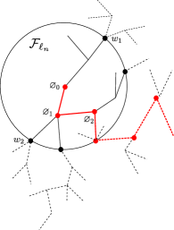
Figure 3: An illustration of the BRW up to $\ell_{n}$. The spine is marked in red. Dotted lines are independent of $\mathcal{F}_{\ell_{n}}$.

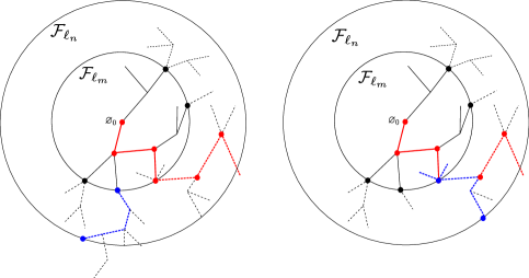
Figure 4: Two illustrations for $V[\varrho_{m}^{(n)},\varrho_{n}]$ (marked in blue).

The following description of the law of $V[\varrho^{(n)}_{m},\varrho_{n}]$ is therefore immediate:

Lemma 4.9.

Let $1\leq m<n$. Under $\mathbf{P}^{({\mathcal{T}}_{\infty})}$, conditioned on ${\mathscr{F}}_{\ell_{m}}$, denote $\ell_{m}=\{w_{1},\cdots,w_{k}\}$ in lexicographical order and $y_{i}=V(w_{i})$ for $1\leq i\leq k$ (with $k=\#\ell_{n}\geq 1$). Then there exists some positive (random, ${\mathscr{F}}_{\ell_{m}}$-measurable) numbers $(p_{i})_{1\leq i\leq k}$, such that $p_{1}+\cdots+p_{k}=1$ and

• with probability $p_{i}\,(1\leq i<k)$, $V[\varrho^{(n)}_{m},\varrho_{n}]$ is distributed as $V[0,\varrho_{n}]$ under ${\bf P}_{y_{i}}^{({\mathcal{T}})}(\bullet\,|\,\varrho_{n}<\infty)$, the critical BRW started at $y_{i}$ and conditioned on exit from $\mathtt{Ball}(n)$;

• with probability $p_{k}$, $V[\varrho^{(n)}_{m},\varrho_{n}]$ is distributed as $V[0,\varrho_{n}]$ under $\mathbf{P}^{({\mathcal{T}}_{\infty})}_{y_{k}}$, the BRW indexed by ${\mathcal{T}}_{\infty}$ and started at $y_{k}$.

More specifically, let for $1\leq i\leq k-1$, $A_{i}$ be the event that the BRW induced by the subtree rooted at $w_{i}$, hits $\mathtt{Ball}(n)$. Then $p_{1}:=\mathbf{P}^{({\mathcal{T}}_{\infty})}(A_{1}|{\mathscr{F}}_{\ell_{m}}),p_{2}:=\mathbf{P}^{({\mathcal{T}}_{\infty})}(A_{2}\cap A_{1}^{c}|{\mathscr{F}}_{\ell_{m}})=\mathbf{P}^{({\mathcal{T}}_{\infty})}(A_{2}|{\mathscr{F}}_{\ell_{m}})\mathbf{P}^{({\mathcal{T}}_{\infty})}(A_{1}^{c}|{\mathscr{F}}_{\ell_{m}}),...,$ $p_{k-1}:=\mathbf{P}^{({\mathcal{T}}_{\infty})}(A_{k-1}\cap A_{1}^{c}\cdots\cap A_{k-2}^{c}|{\mathscr{F}}_{\ell_{m}})$ , and $p_{k}:=1-p_{1}-\cdots-p_{k-1}$.

We end this subsection by a technical estimate on the overshoot of $V$. Let

$$E_{n}:=\Big{\{}\max_{w\in\ell_{n}}|V(w)|\leq 2n\Big{\}},\qquad F_{n}:=\Big{\{}V{[0,\varrho_{n}]}\subset\mathtt{Ball}(2n)\Big{\}}.$$ (4.34)

We show that $E_{n}$ and $F_{n}$ hold with overwhelming probability as $n\to\infty$:

Lemma 4.10.

Assume (1.3) and (1.4). Then

$$\mathbf{P}^{({\mathcal{T}}_{\infty})}(E_{n}^{c})+\mathbf{P}^{({\mathcal{T}}_{\infty})}(F_{n}^{c})\to 0,\qquad n\to\infty.$$

Proof.

For any $u\in\mathcal{T}_{\infty}$, let $\Delta V(u):=V(u)-V({\buildrel\leftarrow\over{u}})$ be the displacement of $u$ with respect to its parent ${\buildrel\leftarrow\over{u}}$. Then

$$E^{c}_{n}\subset\Big{\{}\max_{w\in\ell_{n}}|\Delta V(w)|>n\Big{\}},\qquad F_{n}^{c}\subset\{|V(u_{\varrho_{n}})-V(u_{\varrho_{n}-1})|>n\Big{\}}.$$

Let us prove at first ${\bf P}(F_{n}^{c})\to 0$. For any $\varepsilon>0$, by (4.23), there is some $C=C_{\varepsilon}>0$ such that for all large $n\geq n_{0}$, $\mathbf{P}^{({\mathcal{T}}_{\infty})}(\varrho_{n}\leq Cn^{4})\geq 1-\varepsilon$. Then

$$\mathbf{P}^{({\mathcal{T}}_{\infty})}(F_{n}^{c})\leq\mathbf{P}^{({\mathcal{T}}_{\infty})}(|\Delta V(u_{\varrho_{n}})|>n)\leq\varepsilon+\mathbf{P}^{({\mathcal{T}}_{\infty})}(\max_{0\leq i<Cn^{4}}|V(u_{i+1})-V(u_{i})|>n)\to\varepsilon,$$

as $n\to\infty$ by (4.22). This yields that $\limsup_{n\to\infty}\mathbf{P}^{({\mathcal{T}}_{\infty})}(F_{n}^{c})\leq\varepsilon$, hence is zero as $\varepsilon$ can be arbitrarily small.

To deal with $E^{c}_{n}$, we observe that the spine intersects with $\ell_{n}$ at $\varnothing_{J}$ with

$$J=\min\{j\geq 1:|X_{j}|\geq n\},$$

where by a slight abus of notation, $X_{j}:=V(\varnothing_{j}),j\geq 0$ is a random walk on ${\mathbb{Z}}^{d}$ with step distribution $\theta$. Then

$$\mathbf{P}^{({\mathcal{T}}_{\infty})}(|\Delta V(\varnothing_{J})|>n) = {\mathbb{P}}(|X_{J}-X_{J-1}|>n)$$

$$= \sum_{k=1}^{\infty}{\mathbb{P}}(\max_{1\leq i\leq k-1}|X_{i}|\leq n,|X_{k}|>n,|X_{k}-X_{k-1}|>n)$$

$$\leq \sum_{k=1}^{\infty}{\mathbb{P}}(\max_{1\leq i\leq k-1}|X_{i}|\leq n){\mathbb{P}}(|X_{1}|>n)$$

$$= {\mathbb{E}}(J)\,{\mathbb{P}}(|X_{1}|>n).$$

By the standard estimates for hitting time of a random walk, ${\mathbb{E}}(J)\leq Cn^{2}$ so that

$$\mathbf{P}^{({\mathcal{T}}_{\infty})}(|\Delta V(\varnothing_{J})|>n)\leq C\,n^{2}\,{\mathbb{P}}(|X_{1}|>n),\qquad\forall n\geq 1.$$

Now we deal with those $w\in\ell_{n}\backslash\{\varnothing_{J}\}$ such that $|\Delta V(w)|>n$. Each $w$ is the descendant of a tree rooted at $\varnothing_{i}$ for some $0\leq i\leq J-1$. For any $i\geq 0$, let $\kappa_{i}$ be the number of subtrees rooted at $\varnothing_{i}$. Then $(\kappa_{i})_{i\geq 0}$ are i.i.d. with distribution $\mathbf{P}^{({\mathcal{T}}_{\infty})}(\kappa_{1}=k)=\sum_{i=k+1}^{\infty}p_{i}.$ We have

$$1_{E_{n}^{c}}\leq 1_{\{|\Delta V(\varnothing_{J})|\geq n\}}+\sum_{k=1}^{\infty}1_{\{J=k\}}\sum_{i=0}^{k-1}\sum_{j=1}^{\kappa_{i}}\Theta^{(j)}_{i},$$

where for any $i$, $\Theta^{(j)}_{i},j\geq 1$ are i.i.d. and distributed as $\sum_{w\in\ell_{n}({\mathcal{T}})}1_{\{|\Delta V(w)|\geq n\}}$, under ${\bf P}_{V(\varnothing_{i})}^{({\mathcal{T}})}$, and $\ell_{n}({\mathcal{T}})$ is the optional line defined from ${\mathcal{T}}$ in the same way as $\ell_{n}$ does from ${\mathcal{T}}_{\infty}$ [note that $\ell_{n}({\mathcal{T}})$ may be empty]. Conditioned on $\{V(\varnothing_{i})=x\}$, the expectation of $\Theta^{(j)}_{i}$ is equal to

$$\sum_{m=0}^{\infty}{\bf E}_{x}^{({\mathcal{T}})}\sum_{|w|=m}1_{\{|V(w)|>n,|\Delta V(w)|\geq n,\max_{u\in[\varnothing,w)}|V(u)|\leq n\}}$$

$$= \sum_{m=0}^{\infty}{\mathbb{P}}_{x}\Big{(}|X_{m}|>n,|X_{m}-X_{m-1}|\geq n,\max_{0\leq j\leq m-1}|X_{j}|\leq n\Big{)}$$

$$\leq \sum_{m=0}^{\infty}{\mathbb{P}}_{x}\Big{(}\max_{0\leq j\leq m-1}|X_{j}|\leq n\Big{)}{\mathbb{P}}(|X|\geq n)$$

$$= {\mathbb{P}}(|X|\geq n)\,{\mathbb{E}}_{x}(J+1),$$

where in the second equality we have used the fact that for each $|w|=m$, $V(u),u\in[\varnothing,w)$ is distributed as $X_{j},0\leq j\leq m-1$. For the random walk $(X_{j})$, again by the standard estimate on its hitting time we have ${\mathbb{E}}_{x}(J)\leq C\,n^{2},$ for all $|x|\leq n.$ It follows that

$$\mathbf{P}^{({\mathcal{T}}_{\infty})}(E_{n}^{c}) \leq C\,n^{2}\,{\mathbb{P}}(|X|>n)+\mathbf{E}^{({\mathcal{T}}_{\infty})}(\kappa_{0})\,\mathbf{E}^{({\mathcal{T}}_{\infty})}\sum_{k=1}^{\infty}1_{\{J=k\}}\,k\,Cn^{2}{\mathbb{P}}(|X|\geq n)$$

$$= C\,n^{2}\,{\mathbb{P}}(|X|>n)+C^{\prime}{\mathbb{E}}(J)\,n^{2}{\mathbb{P}}(|X|\geq n)$$

$$\leq C^{\prime\prime}n^{4}{\mathbb{P}}(|X|\geq n),$$

which converges to $0$ by the assumption (1.3). This completes the proof. ∎

4.4 Iteration by optional lines

For the SRW $(S_{i})$, denote by $\tau_{n}$ its first exit time of $\mathtt{Ball}(n)$:

$$\tau_{n}:=\min\{i\geq 0:|S_{i}|\geq n\}.$$ (4.35)

Lemma 4.11.

Assume (1.3) and (1.4). In dimensions $d=3,4,5$, for every $\varepsilon>0$, there exists $\delta>0$ such that for all large $n$,

$$1_{E_{n}}\,\mathbf{P}^{({\mathcal{T}}_{\infty})}(\Xi_{n}<\delta\,|\,{\mathscr{F}}_{\ell_{n}})<\varepsilon,$$

where $E_{n}$ is defined in (4.34) and

$$\Xi_{n}:=\inf_{|x|\leq n}{\rm P}^{({\tt S})}_{x}(S[0,\tau_{6n}]\cap V[\varrho_{n}^{(6n)},\varrho_{6n}]\neq\emptyset).$$

Proof.

By Lemma 4.9, conditionally on ${\mathscr{F}}_{\ell_{n}}$, if $\ell_{n}=\{w_{1},...,w_{k}\}$ and $V(w_{i})=y_{i},1\leq i\leq k$, then $V[\varrho_{n}^{(6n)},\varrho_{6n}]$ is distributed as

$\bullet$ with probability $p_{k}$, $V[0,\varrho_{6n}]$ under $\mathbf{P}^{({\mathcal{T}}_{\infty})}_{y_{k}}$;

$\bullet$ with probability $p_{i}$ for $1\leq i<k$, $V[0,\varrho_{6n}]$ under ${\bf P}^{({\mathcal{T}})}_{y_{i}}(\bullet\,|\,\varrho_{6n}<\infty)$.

Therefore,

$$\mathbf{P}^{({\mathcal{T}}_{\infty})}(\Xi_{n}<\delta\,|\,{\mathscr{F}}_{\ell_{n}})=\sum_{i=1}^{k-1}p_{i}\,a_{n}(y_{i})+p_{k}\,b_{n}(y_{k}),$$

with

$$a_{n}(y) := {\bf P}^{({\mathcal{T}})}_{y}\Big{(}\inf_{|x|\leq n}{\rm P}^{({\tt S})}_{x}(S[0,\tau_{6n}]\cap V[0,\varrho_{6n}]\neq\emptyset)<\delta\,\big{|}\,\varrho_{6n}<\infty\Big{)},$$

$$b_{n}(y) := \mathbf{P}^{({\mathcal{T}}_{\infty})}_{y}\Big{(}\inf_{|x|\leq n}{\rm P}^{({\tt S})}_{x}(S[0,\tau_{6n}]\cap V[0,\varrho_{6n}]\neq\emptyset)<\delta\Big{)}.$$

On $E_{n}$, we have $\max_{1\leq i\leq k}|y_{i}|\leq 2n$, then

$$1_{E_{n}}\mathbf{P}^{({\mathcal{T}}_{\infty})}(\Xi_{n}<\delta\,|\,{\mathscr{F}}_{\ell_{n}})\leq\sup_{|y|\leq 2n}\,\max(a_{n}(y),b_{n}(y)).$$

We deal with $\max_{|y|\leq 2n}b_{n}(y)$, and the argument can be easily adapted to $\max_{|y|\leq 2n}a_{n}(y)$. We shift $y$ to the origin, as the original structures of $V$ under $\mathbf{P}^{({\mathcal{T}}_{\infty})}_{y}$ exit from $\mathtt{Ball}(6n)$, the shifted versions at least exit from $\mathtt{Ball}(4n)$. Then for all $|y|\leq 2n$, $\inf_{|x|\leq n}{\rm P}^{({\tt S})}_{x}(S[0,\tau_{6n}]\cap V[0,\varrho_{6n}]\neq\emptyset)$ under $\mathbf{P}^{({\mathcal{T}}_{\infty})}_{y}$, is stochastically larger than $\gamma_{n}$ under $\mathbf{P}^{({\mathcal{T}}_{\infty})}$, where

$$\gamma_{n}:=\inf_{|z|\leq 3n}{\rm P}^{({\tt S})}_{z}(S[0,\tau_{6n}]\cap V[0,\varrho_{4n}]\neq\emptyset).$$

It follows that

$$\max_{|y|\leq 2n}b_{n}(y)\leq\mathbf{P}^{({\mathcal{T}}_{\infty})}(\gamma_{n}<\delta).$$

For any $\varepsilon\in(0,1)$, let $\delta_{1}:=\delta_{1}(\varepsilon)>0$ be as in Lemma 4.6 such that for all large $k$, under $\mathbf{P}^{({\mathcal{T}}_{\infty})}$, with probability at least $1-\frac{\varepsilon}{4}$,

$${\inf_{|x|\leq k}{\rm P}^{({\tt S})}_{x}(S[0,\infty)\cap V{[0,\varrho_{k}]}\neq\emptyset)\geq\delta_{1}}.$$ (4.36)

Now we choose $\alpha=\alpha(\delta_{1})\in(0,1)$ sufficiently small such that

$$\sup_{n\geq 1}\sup_{|x|\geq 6n}{\rm P}^{({\tt S})}_{x}(\tau_{\mathtt{Ball}(2\alpha n)}<\infty)<\frac{\delta_{1}}{2}.$$

Regardless of the BRW, we define

$$c_{1}(\alpha):=\inf_{n\geq n_{0}}\inf_{|z|\leq 3n}{\rm P}^{({\tt S})}_{z}(\tau_{\mathtt{Ball}(2\alpha n)}<\tau_{6n})>0,$$

where $n_{0}=n_{0}(\alpha)$ is some large but fixed integer. Let $n\geq n_{0}$. It follows that

$$\gamma_{n}\geq c_{1}\,\inf_{|x|\leq\alpha n}{\rm P}^{({\tt S})}_{x}(S[0,\tau_{6n}]\cap V[0,\varrho_{\alpha n}]\neq\emptyset).$$ (4.37)

Let as in (4.34)

$$F_{\alpha n}:=\Big{\{}V{[0,\varrho_{\alpha n}]}\subset\mathtt{Ball}(2\alpha n)\Big{\}}.$$

By Lemma 4.10, $\mathbf{P}^{({\mathcal{T}}_{\infty})}(F_{\alpha n}^{c})\leq\frac{\varepsilon}{4}$ for all $n\geq n_{0}$ (we may enlarge $n_{0}$ if necessary). On $F_{\alpha n}$,

$${\rm P}^{({\tt S})}_{x}(S[0,\tau_{6n}]\cap V{[0,\varrho_{\alpha n}]}\neq\emptyset)\geq{\rm P}^{({\tt S})}_{x}(S[0,\infty)\cap V{[0,\varrho_{\alpha n}]}\neq\emptyset)-\frac{\delta_{1}}{2},$$

which in view of (4.36) is larger than $\frac{\delta_{1}}{2}$ with probability at least $1-\frac{\varepsilon}{4}$. It follows from (4.37) that under $\mathbf{P}^{({\mathcal{T}}_{\infty})}$, with probability at least $1-\frac{\varepsilon}{2}$,

$$\gamma_{n}\geq c_{1}\delta_{1}/2.$$

This means that if $\delta<c_{1}\delta_{1}/2$, then $\max_{|y|\leq 2n}b_{n}(y)\leq\frac{\varepsilon}{2}$. We may treat $\max_{|y|\leq 2n}a_{n}(y)$ in the same way by using Corollary 4.8 and obtain the Lemma. ∎

Lemma 4.12.

Assume (1.3) and (1.4). In dimensions $d=3,4,5$, let

$$c(\lambda,n):=\sup_{|x|<\lambda n}{\rm P}^{({\tt S})}_{x}\left(S[0,\tau_{n}]\cap V[0,\varrho_{n}]=\emptyset\right),$$

then for any $M>0$, there exists $\upsilon>0$ such that for any $\lambda\in(0,1)$ small enough,

$$\limsup_{n\rightarrow\infty}\mathbf{P}^{({\mathcal{T}}_{\infty})}_{0}(c(\lambda,n)>\lambda^{\upsilon})<\lambda^{M}.$$

Proof.

Let $\lambda\in(0,1)$ be small. Set $K:=\lfloor\log_{6}\lambda^{-1}\rfloor$ and $m=\lambda n$. Define for $k=0,1,\cdots,K-1$,

$$g(m,k):=\inf_{|x|\leq m6^{k}}{\rm P}^{({\tt S})}_{x}(S[0,\tau_{m6^{k+1}}]\cap V[\varrho_{m6^{k}}^{(m6^{k+1})},\varrho_{m6^{k+1}}]\neq\emptyset).$$

Then

$$c(\lambda,n)\leq\prod_{k=0}^{K-1}(1-g(m,k)).$$

Let

$$E_{k}:=\Big{\{}\max_{w\in\ell_{m6^{k}}}|V(w)|\leq 2m6^{k}\Big{\}},\qquad 0\leq k\leq K-1.$$

Note that $E_{k}$ is measurable with respect to ${\mathscr{F}}_{\ell_{m6^{k}}}$. Let $\varepsilon\in(0,1)$ be some small constant whose value will be chosen later. By Lemma 4.11, there is some small $\delta>0$ such that for all large $n\geq n_{0}(\varepsilon,\delta,\lambda)$,

$$1_{E_{k}}\,\mathbf{P}^{({\mathcal{T}}_{\infty})}(g(m,k)<\delta\,|\,{\mathscr{F}}_{\ell_{m6^{k}}})<\varepsilon,\qquad\forall\,0\leq k\leq K-1.$$ (4.38)

On the event $\{\sum_{k=0}^{K-1}1_{\{g(m,k)\geq\delta\}}>\frac{K}{2}\}$, $c(\lambda,n)\leq(1-\delta)^{K/2}\sim\lambda^{-\frac{1}{2}\log_{6}(1-\delta)}.$ Then if we take $\upsilon:=-\frac{1}{3}\,\log_{6}(1-\delta)$, we have

$${\rm P}^{({\tt S})}(c(\lambda,n)>\lambda^{\upsilon}) \leq \mathbf{P}^{({\mathcal{T}}_{\infty})}\Big{(}\sum_{k=0}^{K-1}1_{\{g(m,k)\geq\delta\}}\leq\frac{K}{2}\Big{)}$$

$$\leq \mathbf{P}^{({\mathcal{T}}_{\infty})}(\cup_{k=0}^{K-1}E_{k}^{c})+\mathbf{P}^{({\mathcal{T}}_{\infty})}\Big{(}\sum_{k=0}^{K-1}1_{E_{k}\cap\{g(m,k)<\delta\}}>\frac{K}{2}\Big{)}.$$

For the first term we use the union bound:

$$\mathbf{P}^{({\mathcal{T}}_{\infty})}(\cup_{k=0}^{K-1}E_{k}^{c})\leq\sum_{k=0}^{K-1}\mathbf{P}^{({\mathcal{T}}_{\infty})}(E_{k}^{c}),$$

which, according to Lemma 4.10, converges to $0$ as $n\to\infty$.

For the second term we use the Chebyshev inequality: for any $s>0$,

$$\mathbf{P}^{({\mathcal{T}}_{\infty})}\left(\sum_{k=0}^{K-1}1_{E_{k}\cap\{g(m,k)<\delta\}}>\frac{K}{2}\right)\leq e^{-sK/2}\,\mathbf{E}^{({\mathcal{T}}_{\infty})}\left[\prod_{k=0}^{K-1}e^{s1_{E_{k}\cap\{g(m,k)<\delta\}}}\right].$$

By using (4.38),

$$\mathbf{E}^{({\mathcal{T}}_{\infty})}\left[e^{s1_{E_{k}\cap\{g(m,k)<\delta\}}}\,\middle|\,{\mathscr{F}}_{\ell_{m6^{k}}}\right]=1+(e^{s}-1)\mathbf{P}^{({\mathcal{T}}_{\infty})}\left(E_{k}\cap\{g(m,k)<\delta\}\,\middle|\,{\mathscr{F}}_{\ell_{m6^{k}}}\right)\leq 1+(e^{s}-1)\varepsilon.$$

Using these inequalities successively for $k=K-1,K-2,...,0$, we see that

$$\mathbf{E}^{({\mathcal{T}}_{\infty})}\left[\prod_{k=0}^{K-1}e^{s1_{E_{k}\cap\{g(m,k)<\delta\}}}\right]\leq(1+(e^{s}-1)\varepsilon)^{K}\leq e^{K(e^{s}-1)\varepsilon}<e^{Ke^{s}\,\varepsilon}.$$

Now for any $M>0$, we may find some $s>0$ large enough such that $e^{-sK/4}\leq\lambda^{M}$. Then we choose and fix $\varepsilon$ small enough such that $\varepsilon\leq\frac{s}{4}e^{-s}$. It follows that

$$\mathbf{P}^{({\mathcal{T}}_{\infty})}\left(\sum_{k=0}^{K-1}1_{E_{k}\cap\{g(m,k)<\delta\}}\geq\frac{K}{2}\right)\leq e^{-sK/2+Ke^{s}\varepsilon}\leq e^{-sK/4}\leq\lambda^{M},$$

ending the proof. ∎

We need an analogue of Lemma 4.12 for fixed time in place of stopping time: Let for $n\geq 1$ and $0<\lambda<1$,

$$\widehat{c}(\lambda,n):=\sup_{|x|<\lambda n}{\rm P}^{({\tt S})}_{x}(\tau_{V[0,n^{4}]}=\infty).$$

Lemma 4.13.

Assume (1.3) and (1.4). In dimensions $d=3,4,5$, for any $M>0$, there exists $\upsilon>0$ such that for any $\lambda\in(0,1)$ small enough,

$$\limsup_{n\rightarrow\infty}\mathbf{P}^{({\mathcal{T}}_{\infty})}(\widehat{c}(\lambda,n)>\lambda^{\upsilon})<\lambda^{M}.$$

Proof.

By Lemma 4.4,

$$\limsup_{n\to\infty}\mathbf{P}^{({\mathcal{T}}_{\infty})}\Big{(}\max_{0\leq i\leq n^{4}}|V(u_{i})|\leq\lambda^{1/2}n\Big{)}\leq C^{\prime}\,e^{-C\lambda^{-1/2}}.$$

On $\{\max_{0\leq i\leq n^{4}}|V(u_{i})|>\lambda^{1/2}n\}$,

$$\widehat{c}(\lambda,n)\leq\sup_{|x|<\lambda n}{\rm P}^{({\tt S})}_{x}\left(\tau_{V[0,\varrho_{\lambda^{1/2}n}]}=\infty\right)\leq c(\lambda^{1/2},\lambda^{1/2}n),$$

thus

$$\mathbf{P}^{({\mathcal{T}}_{\infty})}(\widehat{c}(\lambda,n)>\lambda^{\upsilon})$$

$$\leq \mathbf{P}^{({\mathcal{T}}_{\infty})}\left(\max_{0\leq i\leq n^{4}}|V(u_{i})|\leq\lambda^{1/2}n\right)+\mathbf{P}^{({\mathcal{T}}_{\infty})}\left(c(\lambda^{1/2},\lambda^{1/2}n)>\lambda^{\upsilon}\right)$$

$$\leq C^{\prime}\,e^{-C\lambda^{-1/2}}+\mathbf{P}^{({\mathcal{T}}_{\infty})}\left(c(\lambda^{1/2},\lambda^{1/2}n)>\lambda^{\upsilon}\right).$$

The result follows by taking $\lambda$ small enough and then applying Lemma 4.12. ∎

To prove Theorem 4.1, we need the help of ${\mathcal{T}}_{\infty}^{*}$ again, which requires an analogue of Lemma 4.13 for ${\mathcal{T}}_{\infty}^{*}$. This, however, is nontrivial. Indeed, the main difference of the two models is the spine, whose spatial positions are given by a SRW. But two independent SRWs up to time $n^{4}$ with starting points $O(n)$ distance apart intersect with a positive probability in dimension $d=3$. To avoid this issue, we use the projection trick in the proof of Lemma 4.6 again. Our strategy is to prove Theorem 4.1 for dimension $d=5$ first, based on the following corollary of Lemma 4.13, and then apply the projection trick.

Corollary 4.14.

Assume (1.3) and (1.4). Let for $n\geq 1$ and $0<\lambda<1$,

$$c^{*}(\lambda,n):=\sup_{\begin{subarray}{c}|x|<\lambda n\end{subarray}}{\rm P}^{({\tt S})}_{x}(\tau_{V^{*}[0,n^{4}]}=\infty).$$

In dimensions $d=5$, for any $M>0$, there exist $\upsilon>0$ such that for any $\lambda\in(0,1)$,

$$\limsup_{n\rightarrow\infty}\mathbf{P}^{({\mathcal{T}}_{\infty}^{*})}(c^{*}(\lambda,n)>\lambda^{\upsilon})<\lambda^{M}.$$ (4.39)

Proof of Corollary 4.14.

Let $\tau_{n}:=\min\{i\geq 0:S_{i}\not\in{\mathtt{Ball}}(n)\}$ be the first exit time of $S$ from ${\mathtt{Ball}}(n)$. By [21, Lemma 6.3.7], there exists some positive constant $c$ such that for all large $k$, uniformly in $|x|\leq k/4$ and $y\in\partial{\mathtt{Ball}(k)}$, ${\rm P}^{({\tt S})}_{x}(S_{\tau_{{k}}}=y)\leq c\,{\rm P}^{({\tt S})}_{0}(S_{\tau_{{k}}}=y).$

It follows that for all $\lambda\in(0,1/4)$, $n$ large enough and $|x|\leq\lambda n$, we have

$${\rm P}^{({\tt S})}_{x}(\tau_{V^{*}[0,n^{4}]}=\infty)\leq \sum_{y\in\partial{\mathtt{Ball}(4\lambda n)}}{\rm P}^{({\tt S})}_{x}(S_{\tau_{4\lambda n}}=y){\rm P}^{({\tt S})}_{y}(\tau_{V^{*}[0,n^{4}]}=\infty)$$ (4.40)

$$\leq c\,\sum_{y\in\partial\mathtt{Ball}(4\lambda n)}{\rm P}^{({\tt S})}_{0}(S_{\tau_{4\lambda n}}=y){\rm P}^{({\tt S})}_{y}(\tau_{V^{*}[0,n^{4}]}=\infty).$$

By (4.15), for any $y\in{\mathbb{Z}}^{d}$,

$${\rm P}^{({\tt S})}_{y}(\tau_{V^{*}[0,n^{4}]}=\infty)\leq 1_{\left\{{\tt t}_{0}^{*}\geq\frac{n^{4}}{2}\right\}}+{\rm P}^{({\tt S})}_{y}(\tau_{V[1,n^{4}/2]+X}=\infty)+{\rm P}^{({\tt S})}_{y}(\tau_{\{V(\varnothing_{i}),i\geq 1\}+X}<\infty)$$

$$\leq 1_{\left\{{\tt t}_{0}^{*}\geq\frac{n^{4}}{2}\right\}}+{\rm P}^{({\tt S})}_{y}(\tau_{V[1,n^{4}/2]+X}=\infty)+\sum_{i=1}^{\infty}G^{(d)}(V(\varnothing_{i})+X-y),$$

where in the last inequality we use the fact that for any $z\in{\mathbb{Z}}^{d}$, ${\rm P}^{({\tt S})}_{y}(\exists j\geq 0:S_{j}=z)\leq\sum_{j=0}^{\infty}{\rm P}^{({\tt S})}_{y}(S_{j}=z)=G^{(d)}(z-y).$ Put this into (4.40), we have that

$$c^{*}(\lambda,n)\leq c\,1_{\left\{{\tt t}_{0}^{*}\geq\frac{n^{4}}{2}\right\}}+c\,1_{\left\{|X|\geq{\lambda n}\right\}}+c\max_{|y|\leq 5\lambda n}{\rm P}^{({\tt S})}_{y}(\tau_{V[1,n^{4}/2]}=\infty)$$ (4.41)

$$+c\,\sum_{y\in\partial{\mathtt{Ball}(4\lambda n)}}{\rm P}^{({\tt S})}_{0}(S_{\tau_{\partial{\mathtt{Ball}}{(4\lambda n)}}}=y)\sum_{i=1}^{\infty}G^{(d)}(V(\varnothing_{i})+X-y)$$

$$=: c^{*}_{1}(\lambda,n)+c^{*}_{2}(\lambda,n)+c^{*}_{3}(\lambda,n)+c^{*}_{4}(\lambda,n).$$

As $n\rightarrow\infty$,

$$\mathbf{P}^{({\mathcal{T}}_{\infty}^{*})}(c^{*}_{1}(\lambda,n)+c^{*}_{2}(\lambda,n)>0)\leq\mathbf{P}^{({\mathcal{T}}_{\infty}^{*})}({\tt t}_{0}^{*}\geq{n^{4}}/{2})+\mathbf{P}^{({\mathcal{T}}_{\infty}^{*})}(|X|\geq{\lambda n})\to 0.$$ (4.42)

Note that $c^{*}_{3}(\lambda,n)\leq\widehat{c}(\lambda^{\prime},n^{\prime})=\max_{|y|\leq\lambda^{\prime}n^{\prime}}{\rm P}^{({\tt S})}_{y}(\tau_{V[1,(n^{\prime})^{4}]}=\infty)$ with $\lambda^{\prime}:=10\lambda$, $n^{\prime}:=\lfloor 2^{-1/4}n\rfloor$. By Lemma 4.13, for any $M>0$, there exists $\upsilon^{\prime}>0$ such that for all small $\lambda^{\prime}$, $\limsup_{n^{\prime}\rightarrow\infty}\mathbf{P}^{({\mathcal{T}}_{\infty}^{*})}(\widehat{c}(\lambda^{\prime},n^{\prime})>(\lambda^{\prime})^{\upsilon^{\prime}})<(\lambda^{\prime})^{M+1}$. Let $\upsilon:=\upsilon^{\prime}/2$, then for all small $\lambda>0$,

$$\limsup_{n\rightarrow\infty}\mathbf{P}^{({\mathcal{T}}_{\infty}^{*})}(c^{*}_{3}(\lambda,n)>\lambda^{\upsilon}/2)<\lambda^{M}.$$ (4.43)

For $c^{*}_{4}(\lambda,n)$, note that under ${\bf P}^{({\mathcal{T}}^{*}_{\infty})}$, $(V(\varnothing_{i})+X)_{i\geq 1}$ is distributed as $(X_{i+1})_{i\geq 1}$, a random walk on ${\mathbb{Z}}^{d}$ with step distribution $\theta$. Let $d=5$. There is some constant $c^{\prime}>0$ such that

$${\bf E}^{({\mathcal{T}}^{*}_{\infty})}\Big{(}\sum_{i=1}^{\infty}G^{(d)}(V(\varnothing_{i})+X-y)\Big{)}\leq\sum_{z\in{\mathbb{Z}}^{d}}G^{(d)}_{\theta}(z)\,G^{(d)}(z-y)\leq c^{\prime}(1+|y|)^{-1},$$

where $G^{(d)}_{\theta}(z):=\sum_{n=0}^{\infty}{\mathbb{P}}(X_{n}=z)$, and we cite [31, (1.5a)] for its asymptotic. Hence ${\bf E}^{({\mathcal{T}}^{*}_{\infty})}(c^{*}_{4}(\lambda,n))\leq c\,c^{\prime}\,(1+|4\lambda n|)^{-1},$ which implies that

$$\limsup_{n\rightarrow\infty}\mathbf{P}^{({\mathcal{T}}_{\infty}^{*})}(c^{*}_{4}(\lambda,n)>\lambda^{\upsilon}/2)=0.$$

This together with (4.41), (4.42), and (4.43) yield Corollary 4.14. ∎

Proof of Theorem 4.1.

As explained in the proof of Lemma 4.6, it suffices to show the Theorem for $d=5$, because the result for dimensions $d=3,4$ follows by using the projection

$$(x_{1},x_{2},x_{3},x_{4},x_{5})\mapsto\left\{\begin{array}[]{ll}(x_{1},x_{2},{x_{3}+x_{4}+x_{5}}),&d=3\\ (x_{1},x_{2},x_{3},{x_{4}+x_{5}}),&d=4\end{array}\right..$$

Let $d=5$. We focus on the model ${\mathcal{T}}_{\infty}^{*}$ first.

Fix $0<\zeta<\frac{1}{4}-\frac{1}{q}$. Let $\varepsilon:=\lambda^{1/\zeta}$. By (4.11), there is some constant $a>0$ such that

$$\mathbf{P}^{({\mathcal{T}}_{\infty}^{*})}\big{(}E_{n,\varepsilon}\big{)}\leq C\,\lambda^{a/\zeta},$$

with

$$E_{n,\varepsilon}:=\Big{\{}\max_{0\leq k\leq\frac{1}{\varepsilon}}\max_{0\leq j\leq\varepsilon n}|V(u_{j+k\varepsilon n}^{*})-V(u_{k\varepsilon n}^{*})|\geq\lambda\,n^{1/4}\Big{\}}.$$

On $E^{c}_{n,\varepsilon}$, for any $x$ such that $\mathtt{d}(x,V^{*}[0,n])<\lambda n^{1/4}\}$, there exists some $0\leq k\leq\frac{1}{\varepsilon}$ such that $\mathtt{d}(x,V(u_{k\varepsilon n}^{*}))<2\lambda n^{1/4}\}$. It follows that on $E^{c}_{n,\varepsilon}$,

$$\Theta_{n} := \sup_{\mathtt{d}(x,V^{*}[0,n])<\lambda n^{1/4}}{\rm P}^{({\tt S})}_{x}(\tau_{V^{*}[0,3n/2]}=\infty)$$

$$\leq \max_{0\leq k\leq\frac{1}{\varepsilon}}\sup_{{\mathtt{d}(x,V(u_{k\varepsilon n}^{*}))<2\lambda n^{1/4}}}{\rm P}^{({\tt S})}_{x}(\tau_{V^{*}[k\varepsilon n,k\varepsilon n+n/2]}=\infty).$$

By (4.1), each $V^{*}[k\varepsilon n,k\varepsilon n+n/2]$, shifted by $V(u_{k\varepsilon n}^{*})$, is distributed as $V^{*}[0,n/2]$. Therefore the union bound yields that

$$\mathbf{P}^{({\mathcal{T}}_{\infty}^{*})}(\Theta_{n}\geq\lambda^{\upsilon},E^{c}_{n,\varepsilon}) \leq (1+\frac{1}{\varepsilon})\mathbf{P}^{({\mathcal{T}}_{\infty}^{*})}\Big{(}\sup_{|x|<2\lambda n^{1/4}}{\rm P}^{({\tt S})}_{x}(\tau_{V^{*}[0,n/2]}=\infty)>\lambda^{\upsilon}\Big{)}$$

$$\leq (1+\frac{1}{\varepsilon})\lambda^{M},$$

for all large $n$, where for the last inequality we have applied Corollary 4.14 to an arbitrary constant $M>\frac{1}{\zeta}$ and the corresponding $\upsilon>0$. Then

$$\limsup_{n\to\infty}\mathbf{E}^{({\mathcal{T}}_{\infty}^{*})}(\Theta_{n})\leq\lambda^{\upsilon}+C\,\lambda^{a/\zeta}+(1+\lambda^{-1/\zeta})\lambda^{M}\to 0,\qquad\lambda\to 0,$$

proving the Theorem for ${\mathcal{T}}_{\infty}^{*}$.

To deal with ${\mathcal{T}}_{\infty}$, we apply (4.14) and obtain that for any fixed $\delta>0$, under ${\bf P}^{({\mathcal{T}}^{*}_{\infty})}(\bullet\,|\,{\tt t}_{0}^{*}=0)$, with probability $1-o(1)$, $V[0,n]$ contains $V^{*}[1,(1-\delta)n]$. Therefore the conclusion (4.2) for $V[0,n]$ follows from that of $V^{*}[1,(1-\delta)n]$ under the event $\{{\tt t}_{0}^{*}=0\}$. ∎

4.5 Intersection probabilities: Proof of Theorem 1.3

We are entitled to give the proof of Theorem 1.3:

Proof of Theorem 1.3.

It suffices to compare $R_{n}$ under $\mathbb{P}$ to $V[0,n]$ under $\mathbf{P}^{({\mathcal{T}}_{\infty})}$ in Theorem 4.1, which follows from the arguments in [32, Section 5] for the coupling between the two models.

Indeed, write $R_{n}[0,k]$ for the first $k+1$ positions in $R_{n}$ in lexicographical order, then

$$\mathbb{E}\Big{[}\sup_{\mathtt{d}(x,R_{n}[0,n/2])<\lambda n^{1/4}}{\rm P}^{({\tt S})}_{x}(\tau_{R_{n}}=\infty)\Big{]} \leq \mathbb{E}\Big{[}\sup_{\mathtt{d}(x,R_{n}[0,n/2])<\lambda n^{1/4}}{\rm P}^{({\tt S})}_{x}(\tau_{R_{n}([0,3n/4])}=\infty)\Big{]}$$

$$\leq C\,\mathbf{E}^{({\mathcal{T}}_{\infty})}\Big{[}\sup_{\mathtt{d}(x,V[0,n/2])<\lambda n^{1/4}}{\rm P}^{({\tt S})}_{x}(\tau_{V[0,3n/4]}=\infty)\Big{]},$$

where the last inequality is due to (4.25). Then by Theorem 4.1,

$$\limsup_{n\to\infty}\mathbb{E}\Big{[}\sup_{\mathtt{d}(x,R_{n}[0,n/2])<\lambda n^{1/4}}{\rm P}^{({\tt S})}_{x}(\tau_{R_{n}}=\infty)\Big{]}\to 0,\qquad\lambda\to 0.$$

Since the other half

$$\sup_{\mathtt{d}(x,R_{n}[n/2,n])<\lambda n^{1/4}}{\rm P}^{({\tt S})}_{x}(\tau_{R_{n}}=\infty)$$

can be treated in the same way, the conclusion follows. ∎

Acknowledgements. The authors would like to thank Jean-François Delmas for helpful discussions on ISE.

References

- [1] Asselah, A. and Schapira, B. (2018+). Deviations for the capacity of the range of a random walk. arXiv:1807.02325.
- [2] Asselah, A., Schapira, B. and Sousi, P. (2018). Capacity of the range of random walk on . Trans. Am. Math. Soc., 370 7627–7645.
- [3] Asselah, A., Schapira, B. and Sousi, P. (2019). Capacity of the range of random walk on . Ann. Probab. 47 1447–1497.
- [4] Bai, T. and Hu. Y. (2022). Capacity of the range of branching random walks in low dimensions. Proc. Steklov Inst. Math. 316 Available at arXiv:2104.11898.
- [5] Bai, T. and Wan, Y. (2020+). Capacity of the range of tree-indexed random walk. Ann. Appl. Probab. (to appear) arXiv:2004.06018.
- [6] Barlow, M.T. and Yor, M. (1982). Semimartingale inequalities via the Garsia-Rodemich-Rumsey lemma, and applications to local times. J. Functional Analysis, 49(2):198–229.
- [7] Chung, K.L. (1948). On the maximum partial sums of sequences of independent random variables. Transactions of the American Mathematical Society. Vol. 64, pp. 205–233.
- [8] Csörgő, M. and Révész, P. (1981). Strong Approximations in Probability and Statistics. Akadémiai Kiadó, Budapest.
- [9] Delmas, J.F. (1999). Some properties of the range of super-Brownian motion. Prob. Theory Rel. Fields. 114, 505–547.
- [10] Duquesne, Th. and Le Gall, J.F. (2002). Random trees, Lévy processes and spatial branching processes. Astérisque, tome 281.
- [11] Einmahl, U. (1989). Extensions of results of Komlós, Major, and Tusnády to the multivariate case. J. Multivariate Anal. 28, No. 1, 20–68.
- [12] Gut, A. (2009). Stopped Random Walks, Limit Theorems and Applications. 2nd edition, Springer Science+Business Media, LLC 1988, 2009
- [13] Ibragimov, I.A. and Linnik, Y.V. (1971). Independent and stationary sequences of random variables. Wolters–Noordhoff Publishing, Groningen.
- [14] Hutchcroft, T. and Sousi, P. (2020). Logarithmic corrections to scaling in the four-dimensional uniform spanning tree. arXiv:2010.15830.
- [15] Jagers, P. (1989). General branching processes as Markov fields. Stoch. Proc. Appl. 32 pp 183–212.
- [16] Janson S. and and Marckert, J.F. (2005). Convergence of discrete snakes. J. Theor. Probab., 18(3):615–645.
- [17] Kortchemski, I. (2017). Sub-exponential tail bounds for conditioned stable Bienaymé-Galton-Watson trees. Probab. Theory Rel. Feilds 168 pp. 1–40.
- [18] Lalley, S.P and Shao, Y. (2015). On the maximum displacement of a critical branching random walk. Probab. Theory Related Fields. 162, 71–96.
- [19] Lawler, G.F. (1991). Intersections of Random Walks. Springer Science+Business Media New York.
- [20] Lawler, G.F. (1996). Cut times for simple random walk. Electron. J. Probab., Vol. 1, Paper no.13.
- [21] Lawler, G.F. and Limic, V. (2010). Random walk: A modern introduction. Cambridge University Press.
- [22] Le Gall, J.F. (1999). Spatial Branching Processes, Random Snakes and Partial Differential Equations. Birkhäuser, Basel.
- [23] Le Gall, J.F. (2005). Random trees and applications. Probability Surveys Vol. 2 245–311.
- [24] Le Gall, J.F. and Lin, S. (2015). The range of tree-indexed random walk in low dimensions. Ann. Probab. 43 2701–2728.
- [25] Le Gall, J.F. and Lin, S. (2016). The range of tree-indexed random walk. J. Inst. Math. Jussieu 15 271–317.
- [26] Lin, S. (2014+). The range of tree-indexed random walk with drift. Preprint.
- [27] Marckert, J.F. and Mokkadem, A. (2004). States spaces of the snake and its tour—convergence of the discrete snake. J. Theoret. Probab., 16(4):1015–1046.
- [28] Marzouk, C. (2020). Scaling limits of discrete snakes with stable branching. Ann. Inst. Henri Poincaré - Probabilités et Statistiques. Vol. 56, 502–523.
- [29] Petrov, V.V. (1995). Limit Theorems of Probability Theory. Sequences of independent random variables. Clarendon Press, Oxford.
- [30] Port, S.C. and Stone, C.J. (1978). Brownian motion and classical potential theory. Academic Press, New York, London.
- [31] Uchiyama, K. (1998). Green’s functions for random walks on . P. Lond. Math. Soc. Vol. 77, 215–240.
- [32] Zhu, Q. (2021). On the critical branching random walk III: the critical dimension. Ann. Inst. H. Poincaré Probab. Statist. 57 73–93.