Gravitational-wave echoes from numerical-relativity waveforms via space-time construction near merging compact objects

Abstract

We propose a new approach toward reconstructing the late-time near-horizon geometry of merging binary black holes, and toward computing gravitational-wave echoes from exotic compact objects. A binary black-hole merger spacetime can be divided by a time-like hypersurface into a Black-Hole Perturbation (BHP) region, in which the space-time geometry can be approximated by homogeneous linear perturbations of the final Kerr black hole, and a nonlinear region. At late times, the boundary between the two regions is an infalling shell. The BHP region contains late-time gravitational-waves emitted toward the future horizon, as well as those emitted toward future null infinity. In this region, by imposing no-ingoing wave conditions at past null infinity, and matching out-going waves at future null infinity with waveforms computed from numerical relativity, we can obtain waves that travel toward the future horizon. In particular, the Newman-Penrose $\psi_{0}$ associated with the in-going wave on the horizon is related to tidal deformations measured by fiducial observers floating above the horizon. We further determine the boundary of the BHP region on the future horizon by imposing that $\psi_{0}$ inside the BHP region can be faithfully represented by quasi-normal modes. Using a physically-motivated way to impose boundary conditions near the horizon, and applying the so-called Boltzmann reflectivity, we compute the quasi-normal modes of non-rotating ECOs, as well as gravitational-wave echoes. We also investigate the detectability of these echoes in current and future detectors, and prospects for parameter estimation.

I Introduction

Delayed and repeating gravitational wave echoes emitted by compact-binary mergers Cardoso et al. (2016a, b); Cardoso and Pani (2017), following the main gravitational waves (GWs), can be signatures of: (i) deviations of laws of gravity from general relativity Zhang and Zhou (2018); Dong and Stojkovic (2021), (ii) near-horizon quantum structures surrounding black holes (BHs) Almheiri et al. (2013); Giddings (2016); Oshita and Afshordi (2019); Cardoso et al. (2019a); Wang et al. (2020); Oshita et al. (2020); Abedi et al. (2021); Chakraborty et al. (2022); Chakravarti et al. (2021, 2022), and (iii) the absence of event horizon, namely the existence of horizonless Exotic Compact Objects (ECOs) Mazur and Mottola (2004); Visser and Wiltshire (2004); Damour and Solodukhin (2007); Holdom and Ren (2017); Mathur (2005). We must emphasize that strong arguments (within the context of general relativity and standard model of matter) exist against the existence of echoes and ECOs, including: (i) the ergoregion instability Cardoso et al. (2008); Vicente et al. (2018); Maggio et al. (2017, 2019a), (ii) the formation of a trapped surface due to the pileup of energy near the stable photon orbit Cunha et al. (2017); Keir (2016); Cardoso et al. (2014); Ghosh and Sarkar (2021), (iii) the collapse of ECO due to the gravity of incident GWs Chen et al. (2019); Addazi et al. (2020), and (iv) other nonlinear effects Cardoso and Pani (2019). Nevertheless, if GW echoes do exist, their detection will serve as an important tool to study the physics of BHs or ECOs. A lot of efforts have been made to search for echoes in observed data (see Ref. Abedi et al. (2020) for a thorough review). As a result, constructing accurate waveform models for GW echoes is necessary and timely Conklin and Afshordi (2021); Mukherjee et al. (2022).

If we restrict deviation from general relativity (GR) to be localized near the would-be horizon, then due to Birkhoff’s theorem, the region outside a spherically symmetric ECO can still be described by a Schwarzschild geometry. Consequently, studies of echoes from non-spinning ECOs were mostly based on the black hole perturbation (BHP) theory and the Zerilli-Regge-Wheeler equations Regge and Wheeler (1957); Zerilli (1969). For instance, Cardoso et al. Cardoso et al. (2016a, b) showed that the initial ringdown signal of different ECO models has an universal feature, and is identical to that of a Schwarzschild BH, even though the quasinormal mode (QNM) spectra of ECOs are completely different from the ones of the Schwarzschild BH. This implies that the initial pulse of the ringdown is more related to space-time geometry near the light ring, rather than the formal spectra of QNMs. The following echoes do depend on the structure of the QNM spectra Hui et al. (2019), which is characterized by modes trapped between the ECO surface and the peak of BH potential barrier Cheung et al. (2021). Mark et al. Mark et al. (2017) developed a framework to systematically compute scalar echoes from non-spinning ECOs, in terms of GWs propagating toward the would-be horizon, and transfer functions that convert this horizon-going wave into echoes toward infinity. Testa et al. Testa and Pani (2018) used a Poschl-Teller potential to approximate the BH potential for perturbations, and and derived an analytical echo template. Meanwhile, Ref. Du and Chen (2018) estimated the contribution of GW echoes to stochastic background. In terms of the membrane diagram, Maggio et al. Maggio et al. (2020) and Chakraborty et al. Chakraborty et al. (2022) treated the ECO surface as a dissipative fluid, and related the reflectivity to the bulk and the shear viscosity. Cardoso et al. Cardoso et al. (2019b) studied resonant excitation of the modes of non-spinning ECOs during an extreme-mass-ratio inspiral. More recently, the echoes of fuzzballs Bianchi et al. (2020); Bena and Mayerson (2020) were computed numerically in Ref. Ikeda et al. (2021), and the GW echo from a three-body system was studied in Ref. Fang et al. (2021).

In astrophysical situations, merger remnants usually have non-negligible spins Abbott et al. (2021), hence it is of great practical interest to model echoes from spinning ECOs. Even if GR is valid away from ECOs, the space-time geometry there can deviate significantly from Kerr, having a general multipole structure Geroch (1970); Hansen (1974). Nevertheless, we shall restrict ourselves to Kerr geometry, whose linear perturbation is described by the Teukolsky equation Teukolsky (1972, 1973). An early attempt towards constructing echo waveforms studied scalar perturbations around a Kerr-like wormhole Bueno et al. (2018). Working on a sourceless system, Nakano et al. Nakano et al. (2017) imposed a complete reflecting boundary condition at a constant Boyer-Lindquist radius. Later, the effect of source terms was investigated Sago and Tanaka (2020); Maggio et al. (2021); Micchi and Chirenti (2020); Longo Micchi et al. (2021); Xin et al. (2021); Srivastava and Chen (2021). Sago et al. Sago and Tanaka (2020) and Maggio et al. Maggio et al. (2021) studied main GWs and echoes generated by a particle that plunges into a Kerr black hole. The case of a particle (with scalar charge) sprialing into a Kerr black hole was studied in Ref. Micchi and Chirenti (2020). Refs. Longo Micchi et al. (2021, 2021); Xin et al. (2021); Srivastava and Chen (2021) further introduced the back-reaction of GW emissions on orbital motion.

Recently, Chen et al. Chen et al. (2021) proposed a more physically-motivated boundary condition, by considering the tidal fields experienced by fiducial observers with zero angular momentum orbiting just above the ECO surface. This model established a relation between the ingoing component of the Weyl scalar $\psi_{0}$ and the outgoing piece of the Weyl scalar $\psi_{4}$. Using this new boundary condition, Xin et al. Xin et al. (2021) calculated GW echoes by computing explicitly the $\psi_{4}$ falling down the ECO surface, and converting it to $\psi_{0}$ via the Teukolsky-Starobinsky (TS) identity Starobinsky (1973); Teukolsky and Press (1974). They found weaker echoes than those obtained from other approaches Wang et al. (2020); Maggio et al. (2019b). A flaw in their calculation is that the TS identity is only applicable in the absence of source terms. A direct computation of $\psi_{0}$ propagating toward the ECO surface was later carried out by Srivastava et al. Srivastava and Chen (2021).

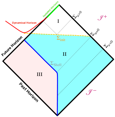
Figure 1: The space-time of a BBH merger event. The hybrid method divides the space-time into an inner PN region (III) and an outer BHP region (I+II). The two regions communicate via boundary conditions at the worldtube $\Sigma_{\rm Shell}$ (the blue curve), which was assumed to track the motion of the BH. The dynamical horizon (the red curve) lies inside the future horizon, and it eventually settles down to the isolated horizon. The common horizon forms at the time slice $\Sigma_{\rm init}$ (the horizontal dashed line). The time slice $\Sigma_{\rm init}$ is not unique and is determined by gauge conditions. The CLA focuses exclusively on the region I, where the system is treated as a Cauchy problem— an initial data needs to be provided on $\Sigma_{\rm init}$, whereas the hybrid method gives attention to both region I and II and handles the system as a boundary value problem.

As we move away from extreme mass ratio inspirals, several approaches have been adopted to model echoes from comparable-mass binary black-hole (BBH) mergers. These include the inside/outside formulations, which do not involve modeling the merger dynamics; the adaptation of the Effective One-Body (EOB) Buonanno and Damour (1999); Han (2014); and the Close-Limit Approximation (CLA) approaches Price and Pullin (1994a); Gleiser et al. (1996); Andrade and Price (1997a); Khanna et al. (1999a), which have played important roles in modeling BBH ringdown waveforms in GR.

In the outside prescription Wang and Afshordi (2018); Conklin and Holdom (2019), the main GR GW emitted by a BBH merger was modeled as having been generated by the reflection of an initial pulse originated from null infinity (see Fig. 1 in Ref. Wang and Afshordi (2018)). The rest of this pulse travels through the light-ring potential, bounces back and forth between the surface of ECO and the peak of the potential. As a result, a sequence of echoes follows the main GR GW at null infinity. In the inside prescription Wang et al. (2020); Maggio et al. (2019b). the main GR GW was modeled instead as the transmitted wave of an initial wave emerging from the past horizon (see Fig. 1 in Ref. Wang et al. (2020)). Wang et al. Wang et al. (2020) computed this initial wave by matching the main GW to that of a BBH merger event, whereas Maggio et al. Maggio et al. (2019b) treated the main pulse as a superposition of QNMs, which led to analytical echo templates. Both the inside and outside prescriptions make direct connections between the main BBH GW and the ensuing echoes; they do not require detailed modeling of the merger dynamics.

In contrast, the approach based on the EOB formulation does rely on the orbital dynamics. Following the same spirit as the EOB method, Micchi et al. Longo Micchi et al. (2021) considered the back-reaction on the orbital evolution due to GW emissions. With a more accurate orbital dynamics, they were able to obtain a complete inspiral-merger-ringdown waveform and the subsequent echoes. Xin et al. Xin et al. (2021) calibrated the dissipative force to a surrogate model Field et al. (2014); Varma et al. (2019) so that the GW at infinity matches the prediction of numerical relativity (NR).

Recently, the CLA approach was applied to computation of echoes from a head-on collision of two equal-mass ECOs Annulli et al. (2021), where the Brill-Lindquist initial data Brill and Lindquist (1963) for two BHs was ported into a linear perturbation of a single Schwarzschild space-time, with a modified boudary condition on a surface right above the horizon.

In addition to the EOB and CLA approaches, a so-called hybrid approach Nichols and Chen (2010, 2012) has also been proposed to jointly use Post-Newtonian (PN) and Black-Hole Perturbation (BHP) theories to model comparable-mass BBH mergers. To illustrate this method, a Penrose diagram of a BBH merger space-time is shown in Fig. 1. The space-time is split by a time-like world tube $\Sigma_{\rm Shell}$ (which asymptotes toward a null tube in its upper-left section) into an inner PN region III and an outer BHP region (I+II). The hybrid approach offers a way to construct space-time geometries in both regions — including GWs at null infinity; it was able to accurately predict the GW waveform and kick velocity of a head-on collision Nichols and Chen (2010, 2012).

In this paper, we shall take a similar point of view as the hybrid approach — by dividing the space-time into a linear BHP region (I and II in Fig. 1) and a region (III) in which the space-time is not a linear perturbation of the remnant BH. We shall not attempt to approximately solve for the entire space-time geometry in all regions, but instead use gravitational waveform at the null infinity $\mathscr{I}^{+}$ already obtained from NR, and reconstruct the space-time geometry in the BHP region — including GWs propagating toward the future horizon $\mathscr{H}^{+}$. In particular, we find the location of the worldtube $\Sigma_{\rm Shell}$ at $\mathscr{H}^{+}$can be determined by looking for when the linearly quasi-normal ringing of horizon GW starts. Equipped with this information, together with the recent physically-motivated boundary condition near the would-be future horizon Chen et al. (2021), we can construct gravitational echoes at $\mathscr{I}^{+}$.

As a first step toward demonstrating our space-time reconstruction approach, in this paper, we restrict ourselves to inspiraling BBHs whose remnants are non-rotating. Specifically, we shall use a NR technique Cauchy-characteristic extraction (CCE) Bishop et al. (1996, 1997); Winicour (2009); Reisswig et al. (2009); Moxon et al. (2020, 2021) to extract the Weyl scalars $\psi_{4}$ and $\psi_{0}$ of the BBH events in question, and use them to reconstruct space-time geometry in the linear BH regions I and II.

This paper is organized as follows. In Sec. II we explain more details about space-time reconstruction using Fig. 1 and outline the basic ideas of the hybrid method. We then describe our NR techniques and simulations in Sec. III. Taking these NR simulations we explicitly carry out space-time reconstruction in Sec. IV, in particular obtaining gravitational waves propagating toward the future horizon $\mathscr{H}^{+}$. With these horizon waveforms, we construct gravitational-wave echoes at $\mathscr{I}^{+}$ in Sec. V. Section VI focuses on the detectability of GW echo and parameter estimation, using the Fisher information matrix formalism. Finally in Sec. VII we summarize our results.

Throughout this paper we use the geometric units with $G=c=1$. Unless stated otherwise, we use the remnant mass $M_{f}$ to normalize all dimensional quantities (e.g., time, length, and Weyl scalars). Note that this choice is different from the typical convention adopted by the NR community, where the initial total mass of the system $M_{\rm tot}$ is used.

II Space-time reconstruction from gravitational waves at future null infinity: theory

In this section, we shall describe our theoretical strategy for space-time reconstruction based on BBH GWs at the future null infinity $\mathscr{I}^{+}$. We shall divide the entire space-time into two regions, the black-hole perturbation region (I+II in Fig. 1), and the strong-field region (III in Fig. 1), as proposed during the construction of the hybrid model for BBH coalescence Nichols and Chen (2010, 2012). In Sec. II.1, we shall review the hybrid method, focusing on how space-time geometry in the bulk of the BHP region depends on boundary values. In Sec. II.2, we discuss in particular how the bulk geometry can be expressed in terms of waves at $\mathscr{I}^{+}$. In Sec. II.3, we focus on GWs that propagate toward the future horizon $\mathscr{H}^{+}$, in particular propose a way to determine the boundary between the BHP region II and the strong field region III. In Sec. II.4, we comment on how our approach is connected to previous works.

II.1 From the hybrid method to space-time reconstruction

In the Penrose diagram of a coalescing BBH space-time (Fig. 1), the red curve represents the dynamical horizon, which is well-known to be inside the event horizon Hawking and Ellis (1973). Nichols and Chen Nichols and Chen (2010) proposed using a 3-dimensional time-like tube $\Sigma_{\rm Shell}$, shown as the blue curve, to divide the space-time into two regions. The exterior regions (I+II) can be treated as a linearly perturbed Schwarzschild spacetime. Interior to the tube $\Sigma_{\rm Shell}$, is a strong field region (III), which Nichols and Chen modeled using post-Newtonian theory; this PN metric is matched to the exterior perturbed Schwarzschild metric on the $\Sigma_{\rm Shell}$. Note that the PN expansion for the interior space-time may break down toward the late stage of evolution, but the shell does fall rapidly to the horizon so the errors might stay within the BH potential and not propagate toward infinity.

For a head-on collision, the tube $\Sigma_{\rm Shell}$ passes through the centers of the two BHs, and follows plunge geodesic of the remnant BH (i.e., the BH on which regions I and II are based). A more sophisticated framework was developed later Nichols and Chen (2012) to determine the motion of $\Sigma_{\rm Shell}$ for an inspiralling BBH system. This framework added a radiation-reaction force to account for the dissipative effect of GW emission. In the end, this PN-BHP system, accompanied by the no-incoming-wave condition at $\mathscr{I}^{-}$, forms a complete set of evolution equations, which leads to an approximated, ab initio waveform model. This method was able to predict a reasonable waveform for a BBH system merging in quasi-circular orbits.

In this paper, we focus mainly on the region I+II, where the space-time is treated as a linear perturbation to a Schwarzschild BH. Let us first examine this linear perturbation using the Sasaki-Nakamura (SN) formalism Sasaki and Tagoshi (2003), in which the SN variable $\tensor{[}_{s}]{{\Psi_{lm}^{\rm SN}}}{}$ satisfies the Regge-Wheeler (RW) equation Regge and Wheeler (1957)

$$\left(\frac{\partial^{2}}{\partial u\partial v}+\frac{V_{\rm RW}^{l}}{4}\right)\tensor{[}_{s}]{{\Psi_{lm}^{\rm SN}}}{}=0,$$ (1)

where $u=t-r_{*}$ and $v=t+r_{*}$ are the retarded and advanced time, respectively, with the tortoise coordinate $r_{*}=r+2\ln\left(\frac{r}{2}-1\right)$. The RW potential reads Leaver (1985)

$$V_{\rm RW}^{l}=\frac{\Delta}{r^{5}}[(l^{2}+l)r-2(s^{2}-1)].$$ (2)

Here $s$ corresponds to the spin weight of $\tensor{[}_{s}]{{\Psi_{lm}^{\rm SN}}}{}$ and $\Delta=r^{2}-2r$. In the hybrid approach, no-incoming wave condition was imposed on $\mathscr{I}^{-}$, while PN data was imposed on $\Sigma_{\rm shell}$. One way to obtain $\tensor{[}_{s}]{{\Psi_{lm}^{\rm SN}}}{}$ throughout regions I+II from these boundary conditions is to use the characteristic method, as we discuss in Appendix B.

In this paper, while keeping the no-incoming condition on $\mathscr{I}^{-}$, we shall revert the rest of the reconstruction process, by imposing outgoing waves obtained from NR on $\mathscr{I}^{+}$(e.g., with the CCE method). In particular, we will obtain perturbative fields near $\mathscr{H}^{+}$, which will inform us the gravitational waveform going down the horizon, and serve as a foundation for obtaining GW echoes.

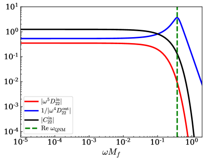
Figure 2: The coefficients $C^{\rm in}_{lm\omega}$ and $D^{\rm in/out}_{lm\omega}$ predicted by the Teukolsky equation, assuming a Schwarzschild BH. The vertical dashed line stands for the real part of the fundamental QNM $(0.374-0.0890i)$. Data are obtained from the Black Hole Perturbation Toolkit BHP .

II.2 Space-time reconstruction using homogeneous Teukolsky solutions

As we reconstruct space-time geometry, instead of SN variables, we will directly consider both $\psi_{0}$ and $\psi_{4}$, because they both have explicit physical meanings, as explained in Ref. Chen et al. (2021). Since the new boundary $\mathscr{I}^{+}$$\cup$ $\mathscr{I}^{-}$for space-time reconstruction has a regular shape (unlike $\Sigma_{\rm shell}$), we can carry out space-time reconstruction by superimposing homogeneous solutions to the Teukolsky equation that already satisfy no-ingoing boundary condition — traditionally referred to as the up solutions.

Let us first write general homogeneous solutions for $\psi_{0}$ and $\psi_{4}$ in mode expansions:

$$\psi_{4}(t,r,\theta,\phi) =\frac{1}{r^{4}}\sum_{lm}\int d\omega\,_{-2}R_{lm\omega}(r)\,{}_{-2}Y_{lm}(\theta,\phi)e^{-i\omega t},$$ (3a)

$$\psi_{0}(t,r,\theta,\phi) =\sum_{lm}\int d\omega\,_{+2}R_{lm\omega}(r)\,{}_{+2}Y_{lm}(\theta,\phi)e^{-i\omega t}.$$ (3b)

Here ${}_{s}Y_{lm}$ are spin-weighted spherical harmonics. The radial functions ${}_{s}R_{lm\omega}(r)$ satisfy the radial Teukolsky equation Teukolsky (1973)

$$\Delta^{-s}\frac{d}{dr}\left(\Delta^{s+1}\frac{d}{dr}\tensor{[}_{s}]{{R_{lm\omega}}}{}\right)+V\tensor{[}_{s}]{{R_{lm\omega}}}{}=0,$$ (4)

with

$$V=4is\omega r-l(l+1)+\frac{r^{4}\omega^{2}-2is(r-M)r^{2}\omega}{\Delta}.$$

The up solutions, with their conventional normalization (with unity outgoing wave amplitude at infinity), have the following asymptotic forms near infinity and horizon

$$\tensor{[}_{-2}]{{R^{\rm up}_{lm\omega}}}{}\sim\begin{cases}r^{3}e^{i\omega r_{*}},\quad&r_{*}\rightarrow+\infty,\\ \\ D^{\rm out}_{lm\omega}e^{i\omega r_{*}}+\Delta^{2}D^{\rm in}_{lm\omega}e^{-i\omega r_{*}},&r_{*}\rightarrow-\infty,\end{cases}$$ (5a)

$$\tensor{[}_{+2}]{{R^{\rm up}_{lm\omega}}}{}\sim\begin{cases}r^{-5}e^{i\omega r_{*}}\,,\quad&r_{*}\rightarrow+\infty,\\ \\ C^{\rm out}_{lm\omega}e^{i\omega r_{*}}+\Delta^{-2}C^{\rm in}_{lm\omega}e^{-i\omega r_{*}},\!\!&r_{*}\rightarrow-\infty.\end{cases}$$ (5b)

Numerical values of the coefficients $C^{\rm in/out}_{lm\omega}$ and $D^{\rm in/out}_{lm\omega}$ are available from the Black-Hole Perturbation Toolkit BHP .

In a BBH coalescence space-time, the $\psi_{0}$ and $\psi_{4}$ in the I+II region have the following asymptotic forms:

$$\tensor{[}_{-2}]{{R^{\rm BBH}_{lm\omega}}}{}\sim\begin{cases}r^{3}Z^{\infty}_{lm\omega}e^{i\omega r_{*}},\quad&r_{*}\rightarrow+\infty,\\ \\ Z^{\rm H\,out}_{lm\omega}e^{i\omega r_{*}}+\Delta^{2}Z^{\rm H\,in}_{lm\omega}e^{-i\omega r_{*}},&r_{*}\rightarrow-\infty,\end{cases}$$ (6a)

$$\tensor{[}_{+2}]{{R^{\rm BBH}_{lm\omega}}}{}\sim\begin{cases}r^{-5}Y^{\infty}_{lm\omega}e^{i\omega r_{*}}\,,\quad&r_{*}\rightarrow+\infty,\\ \\ Y^{\rm H\,out}_{lm\omega}e^{i\omega r_{*}}+\Delta^{-2}Y^{\rm H\,in}_{lm\omega}e^{-i\omega r_{*}},\!\!&r_{*}\rightarrow-\infty.\end{cases}$$ (6b)

Here the amplitudes at infinity, $Z^{\infty}_{lm\omega}$ and $Y^{\infty}_{lm\omega}$ in Eq. (6), can be directly obtained from NR simulations. For completeness, the strain $h_{lm}^{\infty}$ observed at $\mathscr{I}^{+}$ is related to $Z_{lm\omega}^{\infty}$ via

$$h_{lm}^{\infty}(\omega)=\frac{1}{\omega^{2}}Z_{lm\omega}^{\infty}.$$ (7)

Note that $h_{lm}^{\infty}$ is defined later in Eq. (15b). By comparing Eqs. (6) with the standard up solutions in Eqs. (5), we can obtain amplitudes near the horizon:

$$Z^{\rm H\,out}_{lm\omega}=D^{\rm out}_{lm\omega}Z^{\infty}_{lm\omega}\,,\quad Z^{\rm H\,in}_{lm\omega}=D^{\rm in}_{lm\omega}Z^{\infty}_{lm\omega},$$ (8a)

$$Y^{\rm H\,out}_{lm\omega}=C^{\rm out}_{lm\omega}Y^{\infty}_{lm\omega}\,,\quad Y^{\rm H\,in}_{lm\omega}=C^{\rm in}_{lm\omega}Y^{\infty}_{lm\omega}.$$ (8b)

In this way, from waves escaping at infinity, $Z^{\infty}_{{lm\omega}}$ and $Y^{\infty}_{{lm\omega}}$, the coefficients $D^{\rm in}_{lm\omega}$ and $C^{\rm in}_{lm\omega}$ will allow us to reconstruct ingoing waves $Z^{\rm in}_{lm\omega}$ and $Y^{\rm in}_{lm\omega}$ toward $\mathscr{H}^{+}$. We plot $D_{22\omega}^{\rm in}$ and $C_{22\omega}^{\rm in}$ in Fig. 2.

We note that for the same linear perturbative spacetime of Schwarzschild governed by the the vacuum Teukolsky equation, the $\psi_{0}$ and $\psi_{4}$ can be related by the Teukolsky-Starobinsky (TS) relations, which state Starobinsky (1973); Teukolsky and Press (1974):

$$\frac{4\omega^{4}}{C^{*}}Y_{lm\omega}^{\infty}=Z_{lm\omega}^{\infty}\,,\quad$$ (9a)

$$Y_{lm\omega}^{\rm H\,in}=\frac{D}{C}Z_{lm\omega}^{\rm H\,in}$$ (9b)

with

$$C =(l-1)l(l+1)(l+2)+12i\omega$$ (10a)

$$D =64i\omega\left(128\omega^{2}+8\right)\left(1-2i\omega\right).$$ (10b)

These relations are consistent with coefficients in Eqs. (8). For example, because

$$\frac{|C|^{2}}{4\omega^{4}}C^{\rm in}_{lm}=DD^{\rm in}_{lm},$$ (11)

one can obtain $Y^{\rm H\,in}$ from $Z^{\infty}$ either by: (i) using the TS relation at infinity to obtain $Y^{\infty}$, followed by Eq. (8b), or (ii) using Eq. (8a) to obtain $Z^{\rm H\,in}$, and then use the TS relation near the horizon [i.e., Eq. (9b)]. Relations between the BHP quantities have been summarized in Fig. 3. We will check the TS relations directly in Sec. IV.1.

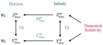
Figure 3: A diagram summarizing relations between BHP quantities on the horizon, $Z^{\rm in}_{lm\omega}$ and $Y^{\rm in}_{lm\omega}$, and those at infinity, $Z^{\infty}_{lm\omega}$ and $Y^{\infty}_{lm\omega}$.

We would like to caution here that while it has been established Starobinsky (1973); Teukolsky and Press (1974) that the TS transformation maps between solutions of $\psi_{0}$ and $\psi_{4}$, these work alone did not explicitly establish the one-to-one relations in Eqs. (9) between $Z_{lm\omega}$ and $Y_{lm\omega}$ for the same GW. Further work by Wald Wald (1978) explicitly related both $\psi_{0}$ and $\psi_{4}$ to the Hertz potential, while more recent work by Loutrel et al. Loutrel et al. (2021) provided a new way to reconstruct metric (hence $\psi_{0}$) from $\psi_{4}$. From Ref. Loutrel et al. (2021), for the same, generic GW, the one-to-one relation is in between $(Z_{l,m,\omega},Z_{l,-m,-\omega})$ and $(Y_{l,m,\omega},Y_{l,-m,-\omega})$, rather than simply between $Z_{lm\omega}$ and $Y_{lm\omega}$. Nevertheless, as will be seen later in this paper (see Sec. IV.1), our numerical results for $\psi_{0}$ and $\psi_{4}$ do agree with Eqs. (9). This might be due to the fact that we have non-precessing systems which satisfy Boyle et al. (2014)

$$Z_{l,m,\omega}=(-1)^{l}Z^{*}_{l,-m,-\omega}\,,\quad Y_{l,m,\omega}=(-1)^{l}Y^{*}_{l,-m,-\omega}\,.$$ (12)

However, for more generic, e.g., precessing binaries, the naive TS relation Eq. (9) may not hold.

II.3 Connection to the inside prescription and determining the location of $\Sigma_{\rm Shell}$

To understand the phyiscal meaning of $Z^{\rm H~{}out}_{lm\omega}$ and $Y^{\rm H~{}out}_{lm\omega}$, which mathematically appears to be emitted from the past horizon $\mathscr{H}^{-}$, we have to go to Fig. 4 and remind ourselves that region I+II does not contain the past horizon of the background BH. Anything below the red curve (the Shell) in Fig. 4 are linear extrapolations. Nevertheless, this extrapolation asserts that waveforms at infinity can be thought of as generated by “image waves” with $Z^{\rm H\,out}$ and $Y^{\rm H\,out}$ that rise from the past horizon. This follows the same reasoning as the inside prescription Wang et al. (2020); Maggio et al. (2019b).

Since the image wave encounters the BH potential barrier (from the inside), it is partially transmitted toward $\mathscr{I}^{+}$, while partially reflected toward $\mathscr{H}^{+}$. We can rewrite

$$Z^{\infty}_{lm\omega}=\frac{1}{D^{\rm out}_{lm\omega}}Z^{\rm H~{}out}_{lm\omega}\,,\quad Z^{\rm H\,in}_{lm\omega}=\frac{D^{\rm in}_{lm\omega}}{D^{\rm out}_{lm\omega}}Z^{\rm H\,out}_{lm\omega}$$ (13a)

$$Y^{\infty}_{lm\omega}=\frac{1}{C^{\rm out}_{lm\omega}}Y^{\rm H~{}out}_{lm\omega}\,,\quad Y^{\rm H\,in}_{lm\omega}=\frac{C^{\rm in}_{lm\omega}}{C^{\rm out}_{lm\omega}}Y^{\rm H\,out}_{lm\omega}$$ (13b)

Here $1/D^{\rm out}_{lm\omega}$ and $1/C^{\rm out}_{lm\omega}$ are the transmissivities from $\mathscr{H}^{-}$to $\mathscr{I}^{+}$, across the potential barrier, while $D^{\rm in}_{lm\omega}/D^{\rm out}_{lm\omega}$ and $C^{\rm in}_{lm\omega}/C^{\rm out}_{lm\omega}$ are reflectivities at the potential barrier that direct the wave toward $\mathscr{H}^{+}$. (The dependence of $1/D^{\rm out}_{22\omega}$ on $\omega$ is plotted in Fig. 2.)

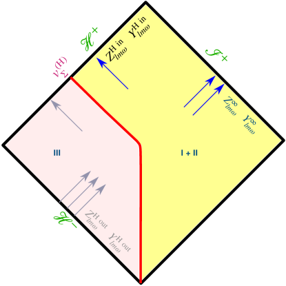
Figure 4: The space-time diagram illustrating the BHP region I+II and their linear extrapolation into region III. Outside the matching shell, curvature perturbations are linear combinations of the up-mode solutions to the homogeneous Teukolsky equation. At the infinity $\mathscr{I}^{+}$, the value of $Z_{lm\omega}^{\infty}$ and $Y_{lm\omega}^{\infty}$ are chosen to be consistent with the predictions of CCE. The past horizon exists in the strong gravity region III, where $Z_{lm\omega}^{\rm H~{}out}$ and $Y_{lm\omega}^{\rm H~{}out}$ represent the image wave that give rise to waves in the region I+II. They serve the same role as the initial wavepacket within the inside prescription Wang et al. (2020); Maggio et al. (2019b). The future horizon lies partially outside the matching shell, only the outside portion $(v>v_{\Sigma}^{(\rm H)})$ of $Z_{lm}^{\rm H~{}in}$ and $Y_{lm}^{\rm H~{}in}$ corresponds to the actual wave that falls down the horizon. One natural way to self-consistently determine the location of $\Sigma_{\rm shell}$ is to evaluate the starting time after which $Y^{\rm H~{}in}_{lm}(v)$ can be decomposed as a sum of QNM overtones. More details can be found in Sec. IV.2.

In this way, we have shown that the inside prescription and the hybrid method correspond to the same reconstruction of space-time geometry in the regime where the linear BHP applies. However, we want to emphasize that two methods adopt different ways when choosing the linear BHP region. In the hybrid method, it is given by the exterior region of $\Sigma_{\rm Shell}$. In particular, in order to compute echoes, we will need to terminate the linear perturbation region at the intersection of the shell $\Sigma_{\rm shell}$ and the future horizon, which is denoted by the advanced time $v=v_{\Sigma}^{({\rm H})}$ in Fig. 4. One natural way to determine the intersection is to first evaluate the time-domain waveform

$$Y^{\rm H~{}in}_{lm}(v)=\int d\omega Y^{\rm H~{}in}_{lm\omega}e^{-i\omega v}$$ (14)

and then define $v_{\Sigma}^{({\rm H})}$ as the starting time after which $Y^{\rm H~{}in}_{lm}(v)$ can be decomposed as a sum of QNM overtones. We shall provide more details when we carry out this decomposition in Sec. IV.2.

On the contrary, the inside prescription uses only the late-time evolution as the linear region. We shall give more discussions regarding this comparison in next subsection (Sec. II.4).

II.4 Further comparisons with the inside prescription and the close limit approximation

To fit the inside prescription into our framework, in Fig. 1, we choose a time slice $\Sigma_{\rm init}$ after which the space-time (i.e., the region I) is consistent with that of a single, perturbed BH. The time slice is usually not unique and is determined by a gauge condition. An appropriate choice is to let $\Sigma_{\rm init}$ represent a moment when the common horizon just forms, following the close limit approximation Price and Pullin (1994b); Abrahams and Price (1996); Andrade and Price (1997b); Khanna et al. (1999b); Sopuerta et al. (2006, 2007); Le Tiec and Blanchet (2010); Johnson-McDaniel et al. (2009). Then the inside prescription corresponds to only taking the region I, and treating it as the linear BHP area. Consequently, one needs to take the ringdown of the main GWs at the null infinity as input, which is equivalent to imposing a filter at $\mathscr{I}^{+}$ Maggio et al. (2019b), and use that information to calculate echoes. In fact, since the region II is not included, the indeterminate condition at past null infinity leaves a room for the outside prescription Wang and Afshordi (2018); Conklin and Holdom (2019).

Similarly, the CLA corresponds to the region I as well. This is an approach to study the space-time based on the fact that the gravitational field in the region I can be modeled as the one of a single perturbed BH. The system in the region I is then treated as a Cauchy problem (i.e., an initial value problem) as long as an initial data is provided on $\Sigma_{\rm init}$. Previous studies have investigated the Misner initial data Misner (1960), the Brill-Lindquist initial data Brill and Lindquist (1963), the Bowen-York initial data Bowen and York (1980) as well as numerically generated initial data Baker et al. (2002); Campanelli et al. (2006). Once the gravitational field in region I is solved, one can read off the value of $Z^{\rm H\,in}_{lm\omega}$ and $Y^{\rm H\,in}_{lm\omega}$ at the future horizon and compute echo waveforms Annulli et al. (2021).

The hybrid method, however, is a boundary value problem. It divides the space-time into two regions via the time-like shell $\Sigma_{\rm Shell}$, as opposed to the space-like hypersurface $\Sigma_{\rm init}$ adopted by the CLA. In addition, both the region I and II are regarded as a BHP area.

III Numerical Relativity simulations

In this section, we adopt two BBH merger simulations performed using the Spectral Einstein Code (SpEC) spe , developed by the Simulating eXtreme Spacetimes (SXS) collaboration Boyle et al. (2019). These binaries have their initial parameters fine-tuned, such that the remnant black holes are nearly non-spinning. Gravitational waveforms (at infinity) of these simulations are publicly available through the SXS catalog Boyle et al. (2019), with the identifier SXS:BBH:0207 and SXS:BBH:1936.

We summarize the properties of these binaries in Table 1, where we adopt the standard convention in SpEC, namely labeling the heavier hole with ‘1’ and the lighter one with ‘2’, and assuming the $z-$axis to be aligned with the initial orbital angular momentum. Our two systems have mass ratios $q=m_{2}/m_{1}=7$, 4, respectively; they undergo $N_{\rm cycle}=36$, 16.5 orbit cycles before the merger, with the initial orbital eccentricity already reduced to $\sim 10^{-4}$. Both systems are non-precessing, with initial spins anti-aligned with the orbital angular momentum (or vanishing), as indicated by the negative signs of the dimensionless spin components, $\chi_{1}^{z}$ and $\chi_{2}^{z}$. The remnant BHs have small spins at the $\chi_{f}\sim 10^{-2}$ level, with the remnant mass $M_{f}$ slightly less than the initial total mass of the system $M_{\rm tot}=m_{1}+m_{2}$.

Table 1: A summary of NR simulations used in this paper. The first column is the identifier in the SXS catalog Boyle et al. (2019). The second column $q=m_{2}/m_{1}>1$ shows the mass ratio. The third column is the number of orbit cycles that a system undergoes before the merger. The fourth and fifth columns give the initial individual dimensionless spins. They have only the $z-$component, where the $z-$axis is chosen to be aligned with the orbital angular momentum. The sixth and seventh columns exhibit the remnant mass (in the unit of initial total mass $M_{\rm tot}$) and remnant spin. The final column corresponds to the radius of the extraction worldtube for CCE.

ID	$q$	$N_{\rm cycle}$	$\chi_{1}^{z}$	$\chi_{2}^{z}$	$\frac{M_{f}}{M_{\rm tot}}$	$\chi_{f}$	Extraction
SXS:BBH:							Radius$(M_{\rm tot})$
0207	7.0	36	$-0.6$	$10^{-6}$	$0.991$	$-0.077$	300
1936	4.0	16.5	$-0.8$	$-0.8$	0.985	$0.022$	273

We extract gravitational waveforms at the null infinity $\mathscr{I}^{+}$ using the Cauchy Characteristic Extraction (CCE) method Moxon et al. (2020, 2021), implemented in the new NR code SpECTRE Kidder et al. (2017); Deppe et al. (2022). The CCE system evolves the Einstein field equations on a foliation of null hypersurfaces, where the metric is written in the Bondi-Sachs coordinates Mädler and Winicour (2016). This method is most efficient in evolving the space-time far from the BBH system, and is reliable enough to produce all Weyl scalars $\psi_{0,1,2,3,4}$ with high accuracy Moxon et al. (2020, 2021). In practice, CCE first reads off boundary data on a worldtube covered by the inner Cauchy evolution, and then evolves a hierarchical system from the worldtube towards future null infinity. The radii of the extraction worldtubes for SXS:BBH:0207 and SXS:BBH:1936 are summarized in Table 1. Same as the standard treatment in NR, CCE decomposes each of the Weyl scalars $\psi_{0,1,2,3,4}$, and the strain $h$, into sums over a set of spin-weighted spherical harmonics $\tensor{[}_{s}]{{Y_{lm}}}{}(\theta,\phi)$. Using the notation defined in Eqs. (6), the decomposition reads

$$[rM_{f}\psi_{4}]_{\mathscr{I}^{+}}=\sum_{l,m}\tensor{[}_{-2}]{{Y_{lm}}}{}(\theta,\phi)Z^{\infty}_{lm},$$ (15a)

$$[rh/M_{f}]_{\mathscr{I}^{+}}=\sum_{l,m}\tensor{[}_{-2}]{{Y_{lm}}}{}(\theta,\phi)h_{lm}^{\infty},$$ (15b)

$$[r^{5}M_{f}^{-3}\psi_{0}]_{\mathscr{I}^{+}}=\sum_{l,m}\tensor{[}_{+2}]{{Y_{lm}}}{}(\theta,\phi)Y^{\infty}_{lm},$$ (15c)

where $\theta$ and $\phi$ are the polar and azimuthal angles, respectively, on the sky in the source frame. Note that in Eqs. (15) the asymptotic $r$-dependences of $\psi_{4}$, $h$ and $\psi_{0}$, as $r\to\infty$, are consistent with the peeling theorem Penrose and Rindler (1984). Furthermore, these fields are normalized by the appropriate powers of $M_{f}$ so that $Z^{\infty}_{lm}$, $Y^{\infty}_{lm}$ and $h_{lm}^{\infty}$ are dimensionless. We want to emphasize again that as opposed to the usual NR convention, where the initial total mass of the system $M_{\rm tot}$ is used as the unit for time and length, in this paper, we use the remnant mass $M_{f}$ to normalize all dimensional quantities, because we mainly deal with perturbations of the remnant (approximately) Schwarzschild BH.

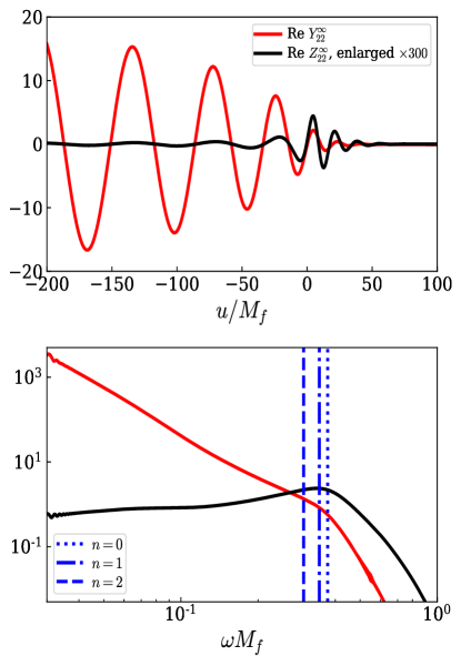
Figure 5: The spherical modes $Y_{22}^{\infty}$ and $Z_{22}^{\infty}$ of SXS:BBH:0207, in the time domain (the upper panel), and in the frequency domain (the lower panel). The vertical lines in the lower panel stand for QNM frequencies of a Schwarzschild BH, labeled by the overtone index $n$. The absolute value of $Z^{\infty}_{22}$ is amplified by a factor of 300 for ease of read.

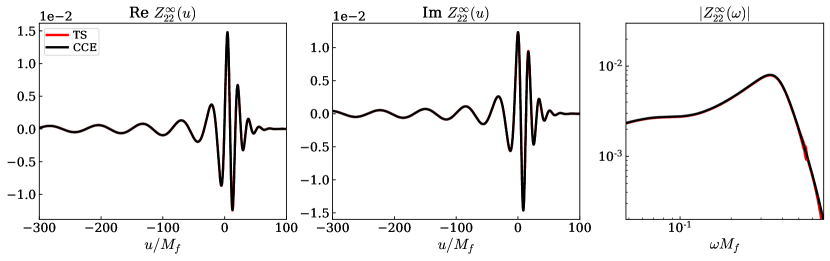
Figure 6: The validity of the TS identity at infinity [Eq. (9a)], using SXS:BBH:0207. The predicted form $\frac{4\omega^{4}}{C^{*}}Y^{\infty}_{22}$ (in red) is compared to the actual $Z^{\infty}_{22}$ (in black), in the time domain (the left two panels), and in the frequency domain (the right panel). The comparison for SXS:BBH:1936 is in Fig. 20.

Furthermore, we shift all temporal coordinates such that $u=0$ corresponds to the peak of total rms strain amplitude:

$$\left.\sqrt{\sum_{lm}|h_{lm}(u)|^{2}}\right|_{u=0}={\rm peak}.$$ (16)

IV Numerical implementations of the hybrid method

In this section, we apply the space-time reconstruction procedure of Sec. II to SXS:BBH:0207 and SXS:BBH:1936. In Sec. IV.1, we first investigate the validity of TS identities at future null infinity $\mathscr{I}^{+}$ [see Eq. (9a)], given that the future null infinity lies completely in the BHP region. We also provide the horizon-$\psi_{0}$ at future horizon $\mathscr{H}^{+}$. Then in Sec. IV.2, we use the horizon-$\psi_{0}$ to determine the location of the matching tube $\Sigma_{\rm Shell}$ by looking for when its linearly quasi-normal ringing starts.

IV.1 At null infinity and future horizon: The Weyl scalars and the Teukolsky-Starobinsky identities

For SXS:BBH:0207, we plot its $Z^{\infty}_{l=2,m=2}$ and $Y^{\infty}_{l=2,m=2}$ in Fig. 5, in both time domain (upper panel) and frequency domain (lower panel). In the frequency domain, $Z^{\infty}_{22}$ (black curve) peaks at the fundamental (2,2) quasi-normal mode frequency (the vertical dotted line). On the other hand, $Y^{\infty}_{22}$ rises up sharply in low frequencies, where its magnitude is much greater than that of $Z^{\infty}_{22}$. This feature in the frequency domain is consistent with the TS identity at infinity [see Eq. (9a)]. To be concrete, we test the validity of Eq. (9a) in Fig. 6. The actual $Z^{\infty}_{22}$ (in black) is compared to $\frac{4\omega^{4}}{C^{*}}Y^{\infty}_{22}$ (in red), in the time domain (the left two panels) and frequency domain (the right panel). We see the TS identity holds throughout the entire region. The comparison for SXS:BBH:1936 is similar and can be found in Appendix C.

At the future horizon, $Y_{lm}^{\rm H\,in}$ [Eq. (6)] is essential for us to compute echoes (see Sec. V.1 for more details). In Fig. 7, we plot $Y_{22}^{\rm H\,in}$ of SXS:BBH:0207 in the time domain (blue curve), where the advanced time $v$ is used as the time coordinate. Similar to $Y^{\infty}_{22}$ [see Fig. 5], $Y_{22}^{\rm H\,in}$ has a dominated low-frequency content. At early stage, $Y_{22}^{\rm H\,in}$ is inside the strong gravity region III and should be excised — as we shall discuss in Secs. IV.2 and V.3. For comparison, we also plot $Y^{\infty}_{22}$ in the same figure (red curve) — using $u$ as the time coordinate. We caution that this comparison only has a qualitative meaning, because the two waveforms are emitted toward different directions. Showing the $v$ dependence of $Y_{22}^{\rm H\,in}$ and the $u$ dependence of $Y^{\infty}_{22}$ in the same plot effectively traces both of these waves back to the same time $t$ at $r_{*}=0$. This is qualitatively meaningful because the ringdown wave can be thought of as having originated from the light ring at $r=3M$, where $r_{*}\approx 0$. From this comparison, we can see $Y_{22}^{\rm H\,in}$ decreases faster and undergoes fewer cycles of oscillation at the late phase than $Y^{\infty}_{22}$.

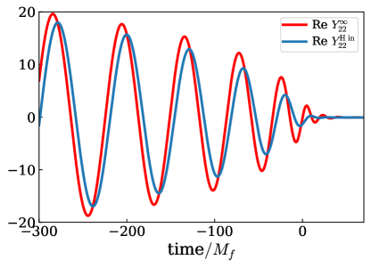
Figure 7: The real part of $Y_{22}^{\rm H\,in}$ [Eq. (6)] and $Y^{\infty}_{22}$ in the time domain, using SXS:BBH:0207. The temporal coordinate for $Y_{22}^{\rm H\,in}$ is $v$, while is $u$ for $Y^{\infty}_{22}$. Both coordinates are in the unit of final mass.

IV.2 Determining the location of $\Sigma_{\rm Shell}$

As mentioned in Sec. II, the region outside the matching tube $\Sigma_{\rm Shell}$ is consistent with a sourceless, linearly perturbed Schwarzschild space-time. Accordingly, the part of $Y_{lm}^{\rm H\,in}$ that is in region I+II can be decomposed into a sum of QNMs (in the time domain). Conversely, we can use this fact to determine the location of $\Sigma_{\rm Shell}$. Indeed, this method has been used not only to determine the start time of a BBH ringdown at the future infinity Giesler et al. (2019), but also to investigate the dynamics of a final apparent horizon in a BBH system approaching to equilibrium Mourier et al. (2021). More specifically, we write Lim et al. (2019),

$$h_{22}^{\infty}(u>u^{(h)})=\sum_{n=0}^{n_{\rm max}}[\mathcal{A}_{n}^{(h)}e^{-i\omega_{n}u}+\mathcal{B}_{n}^{(h)}e^{i\omega_{n}^{*}u}],$$ (17a)

$$Y^{\infty}_{22}(u>u^{(\infty)})=\sum_{n=0}^{n_{\rm max}}[\mathcal{A}_{n}^{(\infty)}e^{-i\omega_{n}u}+\mathcal{B}_{n}^{(\infty)}e^{i\omega_{n}^{*}u}],$$ (17b)

$$Y_{22}^{\rm H\,in}(v>v_{\Sigma}^{({\rm H})})=\sum_{n=0}^{n_{\rm max}}[\mathcal{A}_{n}^{({\rm H})}e^{-i\omega_{n}v}+\mathcal{B}_{n}^{({\rm H})}e^{i\omega_{n}^{*}v}],$$ (17c)

where $\omega_{n}$ is the QNM frequency of a Schwarzchild BH, and $n$ refers to the overtone index (we have restricted to $l=2$). Note that for a Schwarzchild BH, the QNM frequency is independent of its spin weight and azimuthal quantum number. Unlike Ref. Giesler et al. (2019), we include both prograde modes $\mathcal{A}_{n}$ and retrograde modes $\mathcal{B}_{n}$ for generality Dhani (2021). In Eq. (17) we use $u^{(\infty/h)}$ and $v_{\Sigma}^{(\rm H)}$ to indicate the time at which ringdown begins, and we emphasize again that the retarded time $u$ is used for $h_{22}^{\infty}$ and $Y^{\infty}_{22}$ at the null infinity, whereas the advanced time $v$ is used for $Y_{22}^{\rm H\,in}$ at the future horizon .

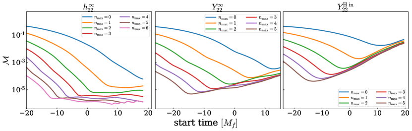
(a) SXS:BBH:0207

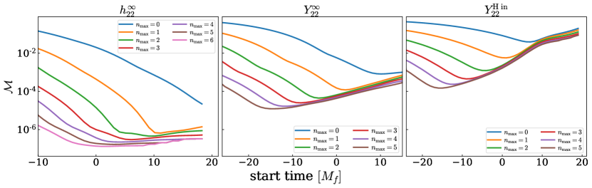
(b) SXS:BBH:1936

Figure 8: Mismatch as a function of start time (in the unit of remnant mass) for different models [Eq. (17)]. Each model includes up to $n_{\rm max}$ overtones. The left panel corresponds to the strain $h_{22}^{\infty}$ at infinity, the middle one $Y_{22}^{\infty}$, and the right panel $Y_{22}^{\rm H\,in}$ [see Eqs. (6) and (15b)]. The upper row refers to SXS:BBH:0207, whereas the lower one SXS:BBH:1936. All waveforms are aligned such that $t=0$ occurs at the peak of $\sqrt{\sum_{lm}|h_{lm}(t)|^{2}}$.

In making the decomposition, we follow the procedure of Ref. Giesler et al. (2019), namely we use the mismatch $\mathcal{M}$ between the quasi-normal mode ringdown waveform model (e.g., $h_{22}^{\rm Ringdown}$) and the NR result (e.g., $h_{22}^{\rm NR}$) as a loss function

$$\mathcal{M}=1-\frac{(h_{22}^{\rm NR},h_{22}^{\rm Ringdown})}{\sqrt{(h_{22}^{\rm Ringdown},h_{22}^{\rm Ringdown})(h_{22}^{\rm NR},h_{22}^{\rm NR})}},$$ (18)

with

$$(h_{22}^{\rm NR},h_{22}^{\rm Ringdown})=\text{Re}\int_{u_{\Sigma}^{(h)}}^{T}h_{22}^{\rm NR}h_{22}^{{\rm Ringdown}~{}*}dt,$$ (19)

where the upper limit of the integral $T$ is taken to be $90M_{f}$ after the peak of total rms strain amplitude. In addition, we use unweighted linear least squares to fit the mode amplitudes and use nonlinear least squares to fit the final spin and mass. The mode frequency $\omega_{n}$ is obtained from a Python package qnm Stein (2019). During the fit, we find that the numerical accuracy of $Y^{\infty}_{22}$ and $Y_{22}^{\rm H\,in}$ is much worse than that of $h^{\infty}_{22}$, which makes the remnant mass and spin more difficult to recover.

In Fig. 8, we plot the mismatch $\mathcal{M}$ for $h_{22}^{\infty}$ (the left panel), $Y_{22}^{\infty}$ (the middle panel), and $Y_{22}^{\rm H\,in}$ (the right panel), for SXS:BBH:0207 (the upper panel) and SXS:BBH:1936 (the lower panel). We see the strain $h_{22}^{\infty}$ can be decomposed into a sum of the fundamental mode and 6 overtones. For SXS:BBH:0207, the linear regime can be extended to $16M_{f}$ before the peak of $h_{22}^{\infty}$, whereas for SXS:BBH:1936, the linear quasinormal ringing regime starts from $2.0M_{f}$, similar to the case of GW150914 Giesler et al. (2019) and superkick systems Ma et al. (2021).

On the other hand, since the numerical accuracy of $Y_{22}^{\infty}$ and $Y_{22}^{\rm H\,in}$ from CCE is not as high as $h_{22}^{\infty}$, only 5 overtones can be resolved. In particular, the late-time portion is dominated by numerical noise, therefore the mismatch $\mathcal{M}$ tends to increase significantly. The start times of the linear regime for $h_{22}^{\infty}$, $Y_{22}^{\infty}$, and $Y_{22}^{\rm H\,in}$ are summarized in Table 2. Below, we will use the start time of $Y_{22}^{\rm H\,in}$, denoted by $v_{\Sigma}^{\rm(H)}$, as the advanced time of the matching tube $\Sigma_{\rm Shell}$ (Figs. 1 and 4), and utilize the exterior portion of the GW to approximate the actual wave falling down the future horizon.

Apart from searching for the start time of quasi-normal ringing regime of $Y_{22}^{\rm H\,in}$, it is also interesting to investigate their QNM amplitudes Oshita (2021); Ma et al. (2021). This topic is beyond the scope of our study and we only provide a brief discussion in Appendix A.

Table 2: A summary for the QNM decomposition of $h_{22}^{\infty}$, $Y_{22}^{\infty}$ and $Y_{22}^{\rm H\,in}$. The second row refers to the maximum number of overtones that we include into Eq. (17). The third and fourth rows correspond to the time from which the waveform is consistent with a linear quasinormal ringing. The values are from the minimum of the corresponding curves in Fig. 8.

		$h_{22}^{\infty}$	$Y_{22}^{\infty}$	$Y_{22}^{\rm H\,in}$
$n_{\rm max}$		6	5	5
$u^{(\infty/h)}$ or $v_{\Sigma}^{(\rm H)}$	SXS:BBH:0207	$-11.1$	$-14.1$	$-13$
	SXS:BBH:1936	$2.0$	$-14.2$	$-15$

V Constructing Echoes

Now we utilize the horizon-going GW obtained above to construct GW echoes at infinity. In Sec. V.1, we first introduce physical boundary conditions near an ECO surface Chen et al. (2021), and obtain formulas that relate horizon waves to echoes at infinity. Then in Sec. V.2, we focus on the Boltzmann reflectivity and discuss QNM structures of the ECO. Next in Sec. V.3, we compute echo waveforms numerically and investigate the impact of prescriptions made at the matching shell $\Sigma_{\rm Shell}$ (see Fig. 1), taking SXS:BBH:0207 for example. Finally, we compare the hybrid method with the inside prescription in Sec. V.4.

V.1 Constructing echoes using the physical boundary condition near an ECO surface

Chen et al. Chen et al. (2021) recently proposed imposing boundary conditions near the ECO surface using the Membrane Paradigm, in which a family of zero-angular-momentum fiducial observers (FIDOs) are considered. Within their own rest frame, the FIDOs experience a tidal tensor field Zhang et al. (2012)

$$\mathcal{E}_{ij}=h^{a}_{i}h^{c}_{j}C_{abcd}U^{b}U^{d},$$ (20)

where $C_{abcd}$ is the Weyl tensor, $U^{b}$ is the four-velocity of the FIDOs, and $h_{i}^{a}=\delta^{a}_{i}+U^{a}U_{i}$ is the projection operator. The transverse component of $\mathcal{E}_{ij}$ is of particular interest Chen et al. (2021)

$$\mathcal{E}_{\rm transverse}\sim-\frac{\Delta}{4r^{2}}\psi_{0}-\frac{r^{2}}{\Delta}\psi_{4}^{*},$$ (21)

since it represents the stretching and squeezing effect due to GW. In analogous to the tidal response of a neutron star, the response of the ECO was proposed to be linear in $\mathcal{E}_{\rm transverse}$, namely Chen et al. (2021)

$$\left[-\frac{r^{2}}{\Delta}\psi_{4}^{*}\right]_{\rm surface}=\left[\frac{\mathscr{R}^{\rm ECO}}{\mathscr{R}^{\rm ECO}-1}\mathcal{E}_{\rm transverse}\right]_{\rm surface}.$$ (22)

The reflectivity $\mathscr{R}^{\rm ECO}$ depends on the (non-GR) property of ECO as we shall discuss in Sec. V.2.

Near the ECO surface, $\psi_{0}$ is dominated by the incident wave (toward the horizon), whereas $\psi_{4}$ by the reflected wave (by the ECO), i.e.,

$$\tensor{[}_{+2}]{{R^{\rm ECO}_{lm}}}{}(u,v)\sim\int\frac{d\omega}{\Delta^{2}}Y_{lm\omega}^{\rm H~{}in~{}ECO}e^{-i\omega v},$$ (23a)

$$\tensor{[}_{-2}]{{R^{\rm ECO}_{lm\omega}}}{}(u,v)\sim\int d\omega Z_{lm\omega}^{\rm H~{}out~{}ECO}e^{-i\omega u},$$ (23b)

with $\tensor{[}_{\pm 2}]{{R^{\rm ECO}_{lm}}}{}(u,v)$ the radial Teukolsky function for the ECO. Here we use the same notation as Eq. (6), and we emphasize that $Y_{lm\omega}^{\rm H~{}in~{}ECO}$ stands for the actual $\psi_{0}$-wave that falls down the future horizon.

After simplification, the boundary condition in Eq. (22) becomes

$$Z_{lm\omega}^{\rm H~{}out~{}ECO}=\frac{(-1)^{l+m+1}}{4}\mathscr{R}^{\rm ECO}Y_{lm\omega}^{\rm H~{}in~{}ECO},$$ (24)

where we have used the symmetry of a nonprecessing BBH system under reflection across the orbital plane Boyle et al. (2014)

$$[Y_{l,-m,-\omega}^{\rm H~{}in~{}ECO}]^{*}=(-1)^{l}Y_{lm\omega}^{\rm H~{}in~{}ECO}.$$ (25)

Subsequently, the echo waveform at null infinity reads Xin et al. (2021)

$$Z_{lm\omega}^{\infty~{}{\rm echo}}=\mathcal{K}(\omega)Y_{lm\omega}^{\rm H~{}in~{}ECO},$$ (26)

with the transfer function $\mathcal{K}(\omega)$

$$\mathcal{K}(\omega)=\frac{(-1)^{l+m+1}\mathscr{R}^{\rm ECO}}{1-\mathscr{R}^{\rm ECO}\mathcal{R}^{\rm BH~{}T}}\frac{1}{4D^{\rm out}_{lm}}=\frac{C}{DD^{\rm in}_{lm}}\sum_{n=1}\left(\mathscr{R}^{\rm ECO}\mathcal{R}^{\rm BH~{}T}\right)^{n},$$ (27)

and

$$\mathcal{R}^{\rm BH~{}T}=(-1)^{l+m+1}\frac{D^{\rm in}_{lm}}{D^{\rm out}_{lm}}\frac{D}{4C}.$$ (28)

In Eq. (27), we have written the total echo signal as a sum of individual echoes.

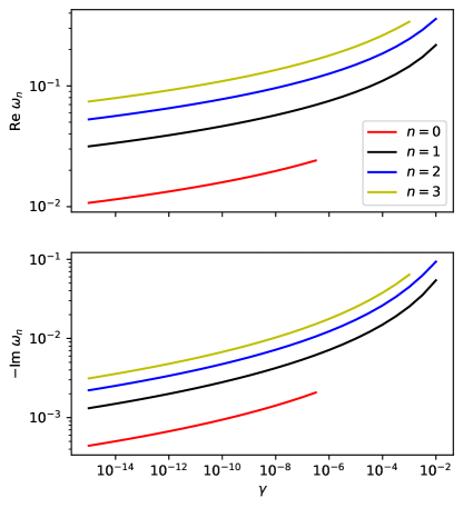
Figure 9: The real and imaginary parts of QNMs for an irrotational ECO, as functions of $\gamma$. They are the solutions to Eq. (31). The Boltzmann reflectivity is used, assuming $T_{\rm QH}=T_{H}$. Each mode is labeled by the overtone index $n$. The imaginary part of QNMs is negative, meaning that the mode is stable.

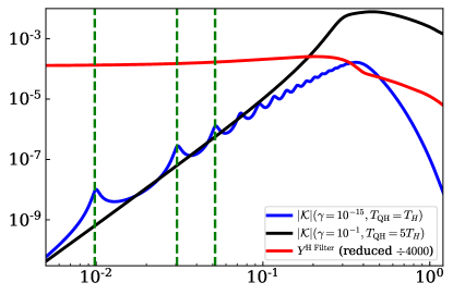
Figure 10: The transfer function $\mathcal{K}$ of the ECO using $(\gamma=10^{-15},T_{\rm QH}=T_{H})$ (the blue curve), and $(\gamma=10^{-1},T_{\rm QH}=5T_{H})$ (the black curve). The QNM resonances are visible in the former case, where the location of first three resonances are labeled by the dashed vertical lines, based on the estimation in Eq. (33). By comparison, the red curve corresponds to the absolute value of the filtered horizon wave $Y^{\rm H~{}Filter}$ for SXS:BBH:0207, assuming $v_{\Sigma}^{\rm H}=-13$ and $\Delta v=2/\kappa$ [see Eq. (36)]. Its value is decreased by a factor of 4000 for ease of read.

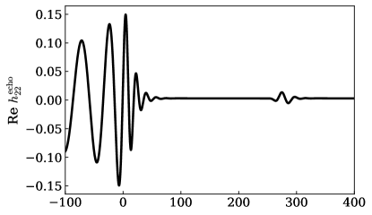
Figure 11: The echo emitted by SXS:BBH:0207, following the main GW. Here we set $v_{\Sigma}^{(\rm H)}=-13,\Delta v=2/\kappa=8,\gamma=10^{-15}$, and $T_{\rm QH}=T_{H}$.

Figure 12: The echoes emitted by SXS:BBH:0207, with a variety of $T_{\rm QH}$ and $\gamma$. The width of filer $\Delta v$ is equal to $2/\kappa$. The total echoes (orange curves) are compared with the first echoes (blue curves). In the upper left panel, the values of $T_{\rm QH}$ and $\gamma$ are small enough that the spacing between echoes is greater than the echo duration, hence the individual pulses are well separated, whereas in the other three panels, different pulses overlap and interfere with each other.

V.2 The Boltzmann reflectivity

To model quantum effects around the horizon, Oshita et al. Oshita et al. (2020) and Wang et al. Wang et al. (2020) proposed that GWs around the horizon interact with a quantum thermal bath. Specifically, these waves are subject to a position-dependent dissipation $\Omega(r_{*})/E_{\rm Pl}$, and driven by a position-dependent stochastic source $\xi(r_{*})$ — levels of the driving and the dissipation are related by the fluctuation-dissipation theorem Kubo (1966). Then the BHP equation is modified to Oshita et al. (2020); Wang et al. (2020)

$$\left[-i\gamma\frac{\Omega(r_{*})}{E_{\rm Pl}}\frac{d^{2}}{dr_{*}^{2}}+\frac{d^{2}}{dr_{*}^{2}}+\omega^{2}-V_{\rm RWZ}^{l}\right]\tensor{[}_{s}]{{\Psi_{lm}^{\rm SN}}}{}(r_{*})=\xi(r_{*}),$$ (29)

where $\Omega(r_{*})=|\omega|/\sqrt{|g_{00}(r_{*})|}$ is the proper frequency measured in the frame of the Schwarzschild observers, $E_{\rm Pl}$ is the Planck energy, and $\gamma$ is a dimensionless dissipation parameter that controls how the damping ramps up as the wave gets close to the horizon. Note that Eq. (29) reduces to the classical Zerilli-RW equation in the limit of $\gamma\to 0$ (vanishing of the dissipative effect) and $\xi\to 0$ (vanishing of the fluctuation source). Consequently, the modified equation leads to the Boltzmann reflectivity Oshita et al. (2020); Wang et al. (2020):

$$\mathscr{R}^{\rm ECO}=\exp\left[-i\frac{\omega}{\pi T_{\rm{QH}}}\ln(\gamma|\omega|)\right]\exp\left(-\frac{|\omega|}{2T_{\rm QH}}\right)\,,$$ (30)

where the quantity $T_{\rm QH}$ is the effective horizon temperature. The first term on the right hand side of Eq. (30) implies that as $\gamma\ll 1$, the region between $r_{*}\sim\frac{\ln\gamma}{2\pi T_{\rm QH}}$ and the peak of the BH potential forms a cavity. In this way, the ECO’s QNM frequencies, $\omega_{n}$, are determined as poles of the transfer function $\mathcal{K}(\omega)$ [see Eq. (27)]

$$\mathscr{R}^{\rm ECO}(\omega_{n})\mathcal{R}^{\rm BH~{}T}(\omega_{n})=1.$$ (31)

We solve Eq. (31) numerically and plot the value of $\omega_{n}$ as a function of $\gamma$ in Fig. 9, where the quantum horizon temperature $T_{\rm QH}$ is set to be the Hawking temperature $T_{H}$:

$$T_{H}\coloneqq\frac{\kappa}{2\pi}=\frac{1}{8\pi},$$ (32)

with $\kappa=1/4$ the surface gravity. We can see that the absolute value of the real and imaginary parts of $\omega_{n}$ increases with $\gamma$ and $n$. In particular, the negative sign of ${\rm Im}~{}\omega_{n}$ ensures the stability of the QNMs. For the fundamental mode $n=0$, its decay rate is less than $10^{-3}$, hence it is long-lived.

The feature of ECO’s QNMs is also visible in the transfer function $\mathcal{K}$, as shown in Fig. 10. The blue curve corresponds to the case with $(\gamma=10^{-15},T_{\rm QH}=T_{H})$. There are a number of local maxima (resonances) whose locations are close to the real part of the corresponding QNMs. In the limit of $\gamma\ll 1$, the peak frequency $\omega^{(n)}_{\rm peak}$ is given by

$$\omega^{(n)}_{\rm peak}=\omega_{\rm FSR}^{(n)}-\frac{\omega_{\rm FSR}^{(n)}}{(2n+1)\pi}{\rm Im}\ln\left[\mathcal{R}^{\rm BH~{}T}(\omega_{\rm FSR}^{(n)})\right],$$ (33)

where the free spectral range (SFR) of the cavity writes

$$\omega_{\rm FSR}^{(n)}=(2n+1)\frac{T_{\rm QH}\pi^{2}}{|\ln\gamma|}\left\{1-\frac{1}{\ln\gamma}\ln\left[(2n+1)\frac{T_{\rm QH}\pi^{2}}{|\ln\gamma|}\right]\right\}$$

$$+\mathcal{O}\left[(\ln\gamma)^{-2}\right],\quad n=0,1\ldots$$ (34)

In Fig. 10 we label the location of $\omega^{(n)}_{\rm peak}$ for $n=0,1,2$ using the dashed vertical lines. Additionally, $\mathcal{K}$ has a global maximum at the fundamental QNM of a Schwarzschild BH $(0.374-0.0890i)$, contributed by the factor $1/D_{22}^{\rm out}$ (see the blue curve in Fig. 2). Within the frequency band $\omega<0.374$, $\mathcal{K}$ is dominated by $1/D_{22}^{\rm out}$, hence its asymptotic behavior is $\sim\omega^{4}$ as $\omega\to 0$. Whereas for the band $\omega>0.374$, $\mathcal{K}$ decays exponentially due to the second term on the right hand side of Eq. (30).

On the other hand, when $\gamma$ is comparable to 1, GWs cannot be effectively trapped near the ECO surface, and the ECO QNMs do not exist. This fact is clearly manifested in the transfer function of the case with $(\gamma=10^{-1},T_{\rm QH}=5T_{H})$, as shown in the black curve in Fig. 10. Moreover, since the value of $T_{\rm QH}$ is greater than the previous one, more high-frequency contents can be reflected by the ECO surface hence emerge at infinity.

Figure 13: The influence of the filter parameter $\Delta v$ on echo waveforms. Each curve corresponds to the real part of the first echo (with different $\Delta v$), using SXS:BBH:0207 and the Boltzmann reflectivity ($\gamma=10^{-15}$ and $T_{\rm QH}=T_{H}$) . The filter is applied at the future horizon with $v_{\Sigma}^{(\rm H)}=-13$.

V.3 Numerical computation of echo waveforms

In order to use Eq. (26) to compute echo waveforms, we first need to estimate the actual wave $Y_{lm\omega}^{\rm H~{}in~{}ECO}$ [see Eq. (23)] that falls down the future horizon. In the context of hybrid method, the future horizon exists partially in region I+II, only the late-time portion of $Y_{lm}^{\rm H~{}in}$ [see Eq. (14)] can represent $Y_{lm}^{\rm H~{}in~{}ECO}$, namely

$$Y_{lm}^{\rm H~{}in~{}ECO}(v)=Y_{lm}^{\rm H~{}in}(v), {\rm when}~{}~{}v>v_{\Sigma}^{({\rm H})}.$$ (35)

Note again that the condition is in the time domain. The value of $v_{\Sigma}^{({\rm H})}$ was determined by searching for the starting time after which $Y_{lm}^{\rm H~{}in}(v)$ can be decomposed as a sum of QNM overtones, as discussed in Sec. IV.2. In practice, we impose the condition in Eq. (35) via a filter:

$$Y_{lm}^{\rm H~{}in~{}ECO}(v) \to Y^{\rm H~{}Filter}_{lm}(v),$$

$$=Y_{lm}^{\rm H~{}in}(v)\mathcal{F}(v)+{\rm Const.}\times[1-\mathcal{F}(v)],$$ (36)

where the Planck-taper filter $\mathcal{F}(v)$ is given by McKechan et al. (2010)

$$\mathcal{F}(v;v_{\Sigma}^{(\rm H)},\Delta v)=\begin{cases}0,&v<v_{\Sigma}^{({\rm H})}-\Delta v,\\ \frac{1}{\exp{z}+1},&v_{\Sigma}^{({\rm H})}-\Delta v<v<v_{\Sigma}^{({\rm H})},\\ 1,&v>v_{\Sigma}^{({\rm H})}.\end{cases}$$ (37)

and $z=\frac{\Delta v}{v-v_{\Sigma}^{({\rm H})}}+\frac{\Delta v}{v-v_{\Sigma}^{({\rm H})}+\Delta v}$. The Planck-taper filter $\mathcal{F}(v)$ is a function that gradually ramps up from 0 to 1 within the time interval $[v_{\Sigma}^{({\rm H})}-\Delta v,v_{\Sigma}^{({\rm H})}]$. Therefore, $Y^{\rm H~{}Filter}_{lm}(v)$ in Eq. (36) represents a quantity that switches from a constant value to $Y_{lm}^{\rm H~{}in}(v)$ that is predicted by the hybrid method. The value of the constant does not affect the echo waveform since this zero-frequency content cannot penetrate the BH potential (see the value of $D_{22}^{\rm out}$ in Fig. 2). In our case, we set the constant to 0.

With the transfer function at hand, we are able to compute echo waveforms. Figure 11 shows an echo signal following the main GW, emitted by the system SXS:BBH:0207, assuming $v_{\Sigma}^{(H)}=-13$, as summarized in Table 2, and $(\Delta v=2/\kappa=8,\gamma=10^{-15},T_{\rm QH}=T_{H})$. To further investigate how the echo signal is impacted by the parameters $(\gamma,T_{\rm QH})$, we vary their values and exhibit the results in Fig. 12. The echo waveform of SXS:BBH:1936 looks similar to that of SXS:BBH:0207, and it can be found in Appendix C. The total echo waveform is compared with the first echo. In the case of $(\gamma=10^{-15},T_{\rm QH}=T_{H})$ (shown in the upper left panel), distinct echo pulses are separated by an equal time interval of

$$\Delta u^{\rm echo}\sim|\ln\gamma|/(\pi T_{\rm QH}),$$ (38)

which is long compared with the duration of BBH ringdown. These well-separated echoes do result mathematically from a collective excitation of ECO’s multiple QNMs displayed in Fig. 10 — even though each individual QNM bears little resemblance to the echo pulse. On the other hand, for greater values of $T_{\rm QH}$ and $\gamma$ ($\gamma=10^{-1},T_{\rm QH}=5T_{H}$, shown in the lower right panel), the spacing between nearby pulses becomes comparable to the pulse duration, distinct echo pulses interfere with each other, and we cannot resolve any single pulse. In addition, since the ECO with greater $T_{\rm QH}$ reflects a broader frequency band, the final echo is stronger.

We then investigate the impact of the filter parameter $\Delta v$ in Eq. (37). As shown in Fig. 13, we compute the first echo emitted by SXS:BBH:0207, using $(\gamma=10^{-15},T_{\rm QH}=T_{H})$ and $v_{\Sigma}^{(\rm H)}=-13$ — for a variety of $\Delta v$. We can see that the waveforms have different amplitude evolution within the first two cycles, but the distinction is suppressed shortly afterwards.

Figure 14: A comparison between the hybrid approach and the inside prescription, using SXS:BBH:0207. We choose the Boltzmann reflectivity with $(\gamma=10^{-15},T_{\rm QH}=T_{H})$. The upper panel shows the first echo, whereas the bottom panel is the second echo. The filter is applied at null infinity (labeled by "Inside", in red), and at future horizon (labeled by "Hybrid", in black). The width of both filter $\Delta v$ is $2/\kappa$.

(a) aLIGO, SXS:BBH:0207

(b) CE, SXS:BBH:0207

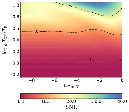
(c) aLIGO, SXS:BBH:1936

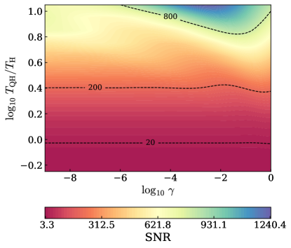
(d) CE, SXS:BBH:1936

Figure 15: The sky-averaged echo SNR across the $T_{\rm QH}-\gamma$ space, using SXS:BBH:0207 (the upper panel) and SXS:BBH:1936 (the lower panel), as well as aLIGO (the left column) and CE (the right column). The binary system is 100Mpc away from the detector, with a total mass of $60M_{\odot}$. We set $\Delta v$ to $2/\kappa$ and the values of $v_{\Sigma}^{(\rm H)}$ are listed in Table 2.

V.4 Comparison with the inside prescription

The horizon filter is absent in the framework of inside prescription Maggio et al. (2019b); Wang et al. (2020). Taking $v_{\Sigma}^{(\rm H)}\to-\infty$, Eq. (35) reduces to

$$Y_{lm\omega}^{\rm H~{}in~{}ECO}=C^{\rm in}_{lm}(\omega)Y^{\infty}_{lm\omega},$$ (39)

and Eq. (26) becomes

$$Z_{lm\omega}^{\infty~{}\rm echo}=\sum_{n=1}^{\infty}\left(\mathscr{R}^{\rm ECO}\mathcal{R}^{\rm BH~{}T}\right)^{n}Z_{lm\omega}^{\infty},$$ (40)

where we have used the TS identities in Eqs. (9). A direct usage of Eq. (40) will lead to undesired low-frequency contents, contributed by the inspiral stage. A workaround would be taking only the ringdown portion of $Z_{lm}^{\infty}(u)$, following Ref. Maggio et al. (2019b). We compare the hybrid method [Eq. (26)] with the inside formula [Eq. (40)] in Fig. 14, assuming SXS:BBH:0207. Here we choose $\Delta v=2/\kappa$ and $(\gamma=10^{-15},T_{\rm QH}=T_{H})$. We see for the first echo, the hybrid method leads to a stronger signal, but the inside prescription has a stronger second echo. Meanwhile, for the initial part of the first echo, the hybrid method gives rise to one more cycle, but the evolution is almost identical afterwards.

VI Detectability and parameter estimation

In this section, we focus on the detectability of the echoes computed in this paper by current and future detectors. We first give a brief summary of detector response, signal-to-noise ratio (SNR) and Fisher matrix calculations in Sec. VI.1. Then we study the detectability of echoes by calculating SNR in Sec. VI.2, and discuss parameter estimation by adopting the Fisher matrix in Sec. VI.3.

VI.1 The signal-to-noise ratio and Fisher-matrix formalism

We first construct two polarizations of an echo $h_{+,\times}^{\rm echo}$ by assembling $h^{\rm echo}_{lm}$:

$$h_{+}^{\rm echo}-ih_{\times}^{\rm echo}=\sum_{m=\pm 2}\tensor{[}_{-2}]{Y}{{}_{l=2,m}}(\theta,\phi)h^{\rm echo}_{l=2,m},$$ (41)

where we are using the leading contributions $h^{\rm echo}_{2,\pm 2}$, who satisfy the condition $h^{\rm echo}_{2,-2}=(h^{{\rm echo}}_{2,2})^{*}$. The echo strain $h^{\rm echo}$ detected by a detector is given by

$$h^{\rm echo}=F_{+}(\theta_{S},\phi_{L},\psi_{L})h_{+}^{\rm echo}+F_{\times}(\theta_{S},\phi_{L},\psi_{L})h_{\times}^{\rm echo},$$ (42)

with $(\theta_{S},\phi_{L})$ the sky location of a source with respect to the detector, and $\psi_{L}$ the polarization angle. The SNR of a given GW signal $h$ is written as $\sqrt{(h|h)}$, where the inner product between two waveforms $(h|g)$ reads

$$(h|g)=4{\rm Re}\int\frac{h^{*}(f)g(f)}{S_{n}(f)}df.$$ (43)

Here $S_{n}(f)$ is the spectral density of the noise when detecting GWs. The averaged SNR over angular parameters $(\theta_{S},\phi_{L},\psi_{L},\theta,\phi)$ is given by Finn and Chernoff (1993)

$$\left<\rho^{2}\right>=\frac{16}{25}\int\frac{|h_{+}|^{2}(\theta=0)}{S_{n}(f)}df.$$ (44)

We shall adopt the sky-averaged SNR all through this paper.

On the other hand, the Fisher matrix for a given gravitational waveform $h(\lambda^{i})$ can be written as

$$\Gamma_{ij}=\left(\left.\frac{\partial h}{\partial\lambda^{i}}\right|\frac{\partial h}{\partial\lambda^{j}}\right),$$ (45)

where $\lambda^{i}$ are parameters to be estimated. In this paper, we restrict ourselves to $(\gamma,T_{\rm QH})$ that determine the Boltzmann reflectivity [Eq. (30)]. By inverting $\Gamma_{ij}$, we obtain parameter estimation accuracies for $\lambda^{i}$ as

$$\Delta\lambda^{i}=\sqrt{(\Gamma^{-1})_{ii}}.$$ (46)

VI.2 Detectability of echoes

To study how the SNR is impacted by the reflectivity parameters $(\gamma,T_{\rm QH})$, we adopt a aLIGO-like detector Aasi et al. (2015) and a Cosmic Explorer (CE)-like detector Abbott et al. (2017), for both SXS:BBH:0207 and SXS:BBH:1936. We assume the binaries to have a total mass of $60M_{\odot}$, and to be located 100Mpc from the detector.

In the baseline case with $T_{\rm QH}=T_{H}$, $\gamma=10^{-1}$, $\Delta v=2/\kappa$ and using values of $v_{\Sigma}^{(\rm H)}$ in Table 2, we obtain (sky-averaged) echo SNR of $\sim 0.45$ for aLIGO, and $\sim 15$ for CE. Echo SNRs of SXS:BBH:1936  are greater than SXS:BBH:0207  by a factor of $\sim 1.5$ in both detectors. In order to compare with Ref. Longo Micchi et al. (2021), we also estimate the ratios between echo SNR and ringdown SNR. To first obtain the ringdown SNR, we choose the lower limit of integration in Eq. (44) to be the frequency of $h_{22}^{\infty}$ evaluated at $u^{(h)}$ [see Eq. (17a) and Table 2]. For aLIGO, the ringdown SNR for SXS:BBH:0207  is around 7.0, and the ratio ${\rm SNR}_{\rm echo}/{\rm SNR}_{\rm ringdown}=6.5\%$, close to the blue curve in the bottom left panel of Fig. 9 in Ref. Longo Micchi et al. (2021).

In Figure 15, we explore how the echo SNR depends on values of $\gamma$ and $T_{\rm QH}$, for both detectors and both binaries, respectively, assuming $\Delta v=2/\kappa$ and the values of $v_{\Sigma}^{(\rm H)}$ being listed in Table 2. The SNR increases with $T_{\rm QH}$ since a larger $T_{\rm QH}$ corresponds to a broader reflection frequency band, and more incident waves are reflected. The $\gamma$ dependence of SNR is more complex. For small values of $T_{\rm QH}$ (i.e., around unity, as originally proposed by Ref. Wang et al. (2020)), the SNR barely depends on $\gamma$, because in this case the echoes are weak and mainly dominated by the first pulse, where $\gamma$ only controls the separation between the echoes in time, then it does not affect the SNR. By contrast, for $T_{\rm QH}\gtrsim 5T_{H}$, the echoes may overlap with each other, and (constructively) interfere, elevating the SNR.

Next we investigate the impact of filters on the horizon, namely the advanced time $v_{\Sigma}^{(\rm H)}$ at which the shell $\Sigma$ crosses the horizon, and the thickness $\Delta v$ of the transition region in which we cut off reflection. Taking SXS:BBH:0207 and CE for example, we plot, in Fig. 16, the sky-averaged echo SNR as a function of two filter parameters $v_{\Sigma}^{(\rm H)}$ and $\Delta v$ [see Eq. (37)], where we choose $\gamma=10^{-15}$ and $T_{\rm QH}=T_{H}$. As expected, the SNR decreases as either $v_{\Sigma}^{(\rm H)}$ increases or $\Delta v$ decreases. The global pattern suggests that the dependence on $v_{\Sigma}^{(\rm H)}$ and $\Delta v$ is linearly correlated.

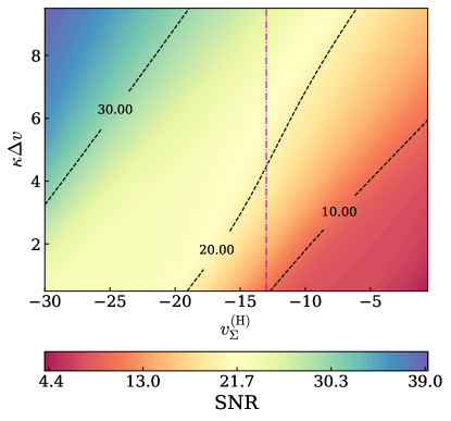
Figure 16: The sky-averaged echo SNR as a function of filter parameters $v_{\Sigma}^{(\rm H)}$ and $\Delta v$ [see Eq. (37)], using CE. The binary system is SXS:BBH:0207 and has the same total mass and distance as Fig. 15. We use the Boltzmann reflectivity with $\gamma=10^{-15}$ and $T_{\rm QH}=T_{H}$. The vertical dot-dashed line stands for the value of $v_{\Sigma}^{(\rm H)}$ in Table 2.

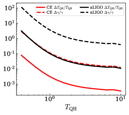
Figure 17: The fractional error of $T_{\rm QH}$ (solid curves) and $\gamma$ (dashed curves) as functions of $T_{\rm QH}$, using aLIGO (in black) and CE (in red). The binary system is SXS:BBH:0207, who has a total mass of $60M_{\odot}$, and is located 100Mpc from the detector. Two filter parameters $v_{\Sigma}^{(\rm H)}$ and $\Delta v$ are still set to $-13$ and $2/\kappa$, respectively. We vary the value of $T_{\rm QH}$ from 0.4 to 10 while fixing the value of $\gamma$ to $10^{-15}$.

VI.3 Parameter estimation

We now use the Fisher-matrix formalism to study parameter estimation. Here we restrict ourselves to reflectivity parameters $(\gamma,T_{\rm QH})$, resulting in 2-D Fisher Matrices. This will result in an under-estimate of measurement errors. As shown in Fig. 17, we compute the fractional errors of $T_{\rm QH}$ and $\gamma$, using SXS:BBH:0207. We still assume that the system has a total mass of $60M_{\odot}$, and is located 100Mpc from the detector. Two filter parameters $v_{\Sigma}^{(\rm H)}$ and $\Delta v$ are still set to $-13$ and $2/\kappa$, respectively. We vary the value of $T_{\rm QH}$ from 0.4 to 10 while fixing the value of $\gamma$ to $10^{-15}$. We see the fractional error decreases as $T_{\rm QH}$ increases, since the echo signal is stronger. The constraint on $T_{\rm QH}$ is greater than $\gamma$ since it has bigger impact on the echo’s profile and SNR. Choosing $T_{\rm QH}=T_{H}$, the aLIGO can constrain $\gamma$ and $T_{\rm QH}$ to the level of 366.7% and 10.2%, respectively. These two constraints lead to 20.9% measurement uncertainty in the time interval $\Delta u^{\rm echo}$ between individual echoes, based on Eq. (38). For CE, the fractional errors of $\gamma$, $T_{\rm QH}$, and $\Delta u^{\rm echo}$ are 11.4% and 0.3%, and 0.65%, respectively.

VII CONCLUSION

In this paper, we made use of the hybrid method Nichols and Chen (2010, 2012) to establish an echo waveform model for comparable-mass merging binaries whose remnants do not rotate. The hybrid method was proposed originally to predict GWs emitted by BBH coalescences — it separates the space-time of a BBH event into an inner PN region and an outer BHP region (see Fig. 1). The two regions communicate via boundary conditions on a worldtube $\Sigma$. To build the echo model, we first took the Weyl scalars of the BBH systems from CCE Moxon et al. (2020) at the future null infinity. Then we reversed the process of the hybrid method by evolving Weyl scalars back into the bulk, and the solution in the BHP region is proportional to the up-mode solution to the homogeneous Teukolsky equation, as required by the uniqueness of solutions. With the solution at hand, we were able to compute the GW that falls down the future horizon.

Since the BHP theory is not valid inside the matching shell $\Sigma$, only the portion of GW that lies outside the worldtube $\Sigma_{\rm Shell}$ is physical. Consequently, the usefulness of our method is limited to the ringdown phase. We determined the location of $\Sigma$, namely the advanced time $v_{\Sigma}^{(\rm H)}$ at which it crosses the future horizon, by looking for the quasi-normal ringing regime of the horizon$-\psi_{0}$ — we fitted $Y^{\rm H~{}in}_{lm}$ to a superposition of five overtones [Eq. (17)]. We then removed the earlier piece of $\psi_{0}$ (with $v<v_{\Sigma}^{(H)}$) by applying a Planck-taper filter, whose width $\Delta v$ (a free parameter in our model) can be viewed as the effective thickness of the matching shell.

Next, by utilizing the physical boundary condition near ECO surfaces Chen et al. (2021) and the Boltzmann reflectivity Wang et al. (2020), we computed the QNMs of irrotational ECOs, as well as echo signals of two systems: SXS:BBH:0207 and SXS:BBH:1936. We picked these two runs because their remnant spins vanish, in which the prediction of the hybrid method for ringdown signals has proved to be accurate Nichols and Chen (2010). Finally, we studied the detectability and parameter estimation of echoes.

We summarize our main conclusions as follows:

(i) The hybrid method is similar to the inside prescription of Refs. Wang et al. (2020); Maggio et al. (2019b) in the sense that both of them treat the main GW as a transmitted wave of an initial pulse emerging from the past horizon (see Fig. 4). Furthermore, filters are involved in both treatments, which, however, have different physical interpretations. The inside prescription (also the CLA) handles the system as an initial value problem (the Cauchy problem), where the whole process is split into two stages. Only the late time portion lies in the BHP region. Therefore, the filter needs to be applied at the future null infinity. Oppositely, in our case, the exterior system is described by a boundary value problem — a spatial volume is separated at every moment. Accordingly, the filter is imposed at the future horizon to remove the unrealistic portion of the incoming GW. We took SXS:BBH:0207 as an example and compared the hybrid method with the inside prescription. We found that the inside prescription leads to fewer cycles than the hybrid method for the initial part of the echo. Meanwhile, the first echo predicted by the inside prescription is weaker than the result by the hybrid method.

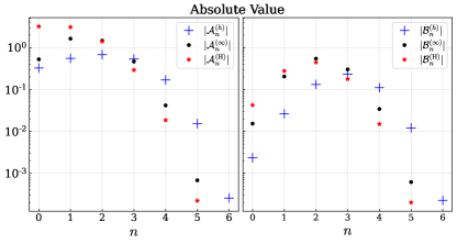
(a) SXS:BBH:0207

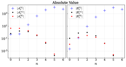
(b) SXS:BBH:1936

Figure 18: The absolute value (the left two panels) and phase (the right two panels) of the prograde mode $\mathcal{A}_{n}$ and the retrograde mode $\mathcal{B}_{n}$, assuming SXS:BBH:0207 (the upper row) and SXS:BBH:1936 (the lower row). We fit Eqs. (17) to the data of $h_{22}^{\infty}$ (blue), $Y_{22}^{\infty}$ (black) as well as $Y_{22}^{\rm H~{}in}$ (red) obtained from CCE.

(ii) The Weyl scalars $\psi_{0,4}$ from CCE are consistent with the TS identities throughout the entire frequency band in question. This supports the treatment of the hybrid method that uses the BHP theory to describe the exterior region, at least when the remnant object does not rotate.

(iii) Similar to the studies of Refs. Giesler et al. (2019); Ma et al. (2021), using six overtones, the ringdown of the strain for SXS:BBH:1936 starts at $2M_{f}$ after the peak. However, the time for SXS:BBH:0207 can be extended to $\sim 11M_{f}$ before the peak. For the horizon and infinity $\psi_{0}$: $Y_{22}^{\rm H/\infty}$, the prediction of CCE is less accurate, and we were only able to resolve five overtones. The linearly quasi-normal ringing regime of $Y_{22}^{\rm H~{}in}$ for SXS:BBH:0207 and SXS:BBH:1936 are similar and they start at $\sim 13-15M_{f}$ before the peak.

We have restricted ourselves to inspiralling compact binaries whose remnants are Schwarzschild-like ECOs. Future work could extend the hybrid method to Kerr-like ECOs and utilize it to compute echoes emitted by more general comparable-mass coalescence systems. It is worth pointing out that throughout the process, the Kerr-like background should have an adiabatically evolving mass and angular momentum due to GW emission. It will be a limitation for the hybrid method if one fails to capture this feature. Another possible avenue for future work is to apply our calculations to head-on collisions and compare the echo waveform with the results in Ref. Annulli et al. (2021).

Appendix A The QNM amplitudes of SXS:BBH:0207 and SXS:BBH:1936

Figure 18 shows the absolute value and phase of $\mathcal{A}^{(h/\infty/\rm H)}_{n}$ and $\mathcal{B}^{(h/\infty/\rm H)}_{n}$ [see Eq. (17)]. For SXS:BBH:1936, $\mathcal{A}_{n}^{(h)}$ peaks at $n=5$, consistent with previous studies Giesler et al. (2019); Ma et al. (2021); Oshita (2021). However, in this case the absolute value of the retrograde mode $\mathcal{B}^{(h)}_{n}$ is comparable with that of $\mathcal{A}_{n}^{(h)}$, thus it is not negligible. For SXS:BBH:0207, the contribution of the retrograde mode $\mathcal{B}_{n}^{(h)}$ is considerable as well, and $\mathcal{A}_{n}^{(h)}$ peaks at $n=2$ and $\mathcal{B}_{n}^{(h)}$ at $n=3$.

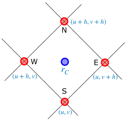
Figure 19: The $(u,v)$ grid cell in characteristic evolution scheme for the RW equation.

Appendix B The characteristic approach for solving the RW equation

Eq. (1) can be solved numerically via a second-order-accurate, characteristic method, proposed by Gundlach et al. Gundlach et al. (1994). As shown in Fig. 19, Gundlach et al. Gundlach et al. (1994) picked four points on a discretized $(u,v)$ grid:

$$\tensor{[}_{s}]{{\Psi_{lm}^{\rm N}}}{}=\tensor{[}_{s}]{{\Psi_{lm}^{\rm SN}}}{}(u+h,v+h), \tensor{[}_{s}]{{\Psi_{lm}^{\rm E}}}{}=\tensor{[}_{s}]{{\Psi_{lm}^{\rm SN}}}{}(u,v+h),$$

$$\tensor{[}_{s}]{{\Psi_{lm}^{\rm W}}}{}=\tensor{[}_{s}]{{\Psi_{lm}^{\rm SN}}}{}(u+h,v), \tensor{[}_{s}]{{\Psi_{lm}^{\rm S}}}{}=\tensor{[}_{s}]{{\Psi_{lm}^{\rm SN}}}{}(u,v),$$ (47)

with $h$ the step size. The value on left corner $\tensor{[}_{s}]{{\Psi_{lm}^{\rm W}}}{}$ can be obtained through

$$\tensor{[}_{s}]{{\Psi_{lm}^{\rm W}}}{}= \tensor{[}_{s}]{{\Psi_{lm}^{\rm N}}}{}+\tensor{[}_{s}]{{\Psi_{lm}^{\rm S}}}{}-\tensor{[}_{s}]{{\Psi_{lm}^{\rm E}}}{}$$

$$+\frac{h^{2}}{8}V^{l}_{\rm RW}(r_{c})(\tensor{[}_{s}]{{\Psi_{lm}^{\rm N}}}{}+\tensor{[}_{s}]{{\Psi_{lm}^{\rm S}}}{})+\mathcal{O}(h^{3}),$$ (48)

where $V^{l}_{\rm RW}(r_{c})$ is the value of the RW potential at the center $r_{c}=(u+h/2,v+h/2)$. We note that Eq. (48) is different from the one used in Refs. Nichols and Chen (2010, 2012), where $\tensor{[}_{s}]{{\Psi_{lm}^{\rm N}}}{}$ was calculated based on the other three. This is because we evolve the system backward into the bulk (from $\mathscr{I}^{+}$ to past horizon).

Appendix C SXS:BBH:1936

Using SXS:BBH:1936, we test the validity of the TS identity at the null infinity [see Eq. (9a)] in Fig. 20. Conventions are the same as Fig. 6.

In Fig. 21, we present the total echo and the first echo with a variety of $(\gamma,T_{\rm QH})$. The location of the filter is listed in Table 2, and the width of the filter is set to $2/\kappa$.

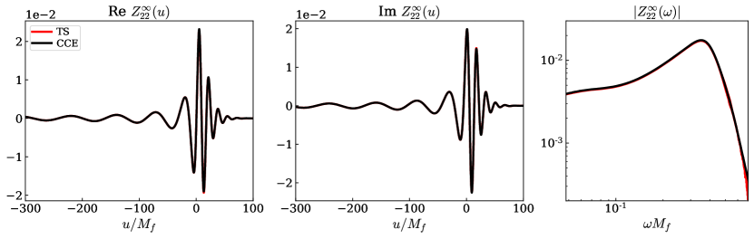
Figure 20: Same as Fig. 6, using SXS:BBH:1936.

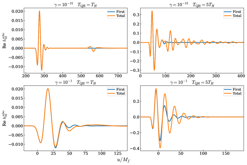
Figure 21: Same as Fig. 12, using SXS:BBH:1936.

Appendix D Chandrasekhar–Sasaki–Nakamura transformation

The generalized Chandrasekhar–Sasaki–Nakamura transformation reads Hughes (2000)

$$\tensor{[}_{s}]{{\Psi_{lm}^{\rm SN}}}{}=\begin{cases}r^{|s|+1}D_{-}^{|s|}\left(\frac{1}{r^{|s|}}\tensor{[}_{s}]{{R^{\rm BH}_{lm}}}{}\right)&s<0,\\ r^{s+1}D_{+}^{s}\left[\left(\frac{\Delta}{r}\right)^{s}\tensor{[}_{s}]{{R^{\rm BH}_{lm}}}{}\right]&s\geq 0,\end{cases}$$ (49a)

$$\tensor{[}_{s}]{{R^{\rm BH}_{lm}}}{}=\begin{cases}\frac{1}{c_{0}}\left(\frac{\Delta}{r}\right)^{|s|}D_{+}^{|s|}\left(r^{|s|-1}\tensor{[}_{s}]{{\Psi_{lm}^{\rm SN}}}{}\right)&s\leq 0,\\ \frac{1}{c_{0}}\frac{1}{r^{s}}D_{-}^{s}\left(r^{s-1}\tensor{[}_{s}]{{\Psi_{lm}^{\rm SN}}}{}\right)&s>0,\end{cases}$$ (49b)

with $D_{\pm}=\frac{d}{dr}\pm\frac{i\omega r^{2}}{\Delta}$ and the constant $c_{0}$ given by

$$c_{0}=\begin{cases}C^{*}&s=-2,\\ l(l+1)&s=\pm 1,\\ C&s=2,\end{cases}$$

where $C$ is defined in Eq. (10a).

The up-mode solution, $\tensor{[}_{s}]{{\Psi_{lm\omega}^{\rm up}}}{}$, to the RW equation [Eq. (1)] takes an asymptotic expansion:

$$\tensor{[}_{-2}]{{\Psi_{lm\omega}^{\rm up}}}{}\sim\begin{cases}B^{\infty}_{lm\omega}e^{i\omega r_{*}}\,,\quad&r_{*}\rightarrow+\infty,\\ \\ B^{\rm out}_{lm\omega}e^{i\omega r_{*}}+B^{\rm in}_{lm\omega}e^{-i\omega r_{*}}\,,\quad&r_{*}\rightarrow-\infty,\end{cases}$$ (50a)

$$\tensor{[}_{+2}]{{\Psi_{lm\omega}^{\rm up}}}{}\sim\begin{cases}A^{\infty}_{lm\omega}e^{i\omega r_{*}}\,,\quad&r_{*}\rightarrow+\infty,\\ \\ A^{\rm out}_{lm\omega}e^{i\omega r_{*}}+A^{\rm in}_{lm\omega}e^{-i\omega r_{*}}\,,\quad&r_{*}\rightarrow-\infty.\end{cases}$$ (50b)

Plugging Eqs. (5) and (50) into Eq. (49), we obtain

$$B^{\infty}_{lm\omega}=-\frac{C^{*}}{4\omega^{2}}, B^{\rm out}_{lm\omega}=-\frac{C^{*}D^{\rm out}_{lm}}{8\omega(i+4\omega)},$$

$$B^{\rm in}_{lm\omega}=16(1-6i\omega-8\omega^{2})D^{\rm in}_{lm},$$

$$A^{\infty}_{lm\omega}=-4\omega^{2}, A^{\rm in}_{lm\omega}=\frac{C}{8\omega(i-4\omega)}C^{\rm in}_{lm},$$

$$A^{\rm out}_{lm\omega}=16(1+6i\omega-8\omega^{2})C^{\rm out}_{lm},$$ (51a)

and the TS identity in Eq. (11) implies

$$\frac{B^{\rm in}_{lm\omega}}{B^{\infty}_{lm\omega}}=\frac{A^{\rm in}_{lm\omega}}{A^{\infty}_{lm\omega}}.$$ (52)

References

- Cardoso et al. (2016a) V. Cardoso, E. Franzin, and P. Pani, Phys. Rev. Lett. 116, 171101 (2016a), [Erratum: Phys.Rev.Lett. 117, 089902 (2016)], arXiv:1602.07309 [gr-qc] .
- Cardoso et al. (2016b) V. Cardoso, S. Hopper, C. F. B. Macedo, C. Palenzuela, and P. Pani, Phys. Rev. D 94, 084031 (2016b), arXiv:1608.08637 [gr-qc] .
- Cardoso and Pani (2017) V. Cardoso and P. Pani, Nature Astron. 1, 586 (2017), arXiv:1709.01525 [gr-qc] .
- Zhang and Zhou (2018) J. Zhang and S.-Y. Zhou, Phys. Rev. D 97, 081501 (2018), arXiv:1709.07503 [gr-qc] .
- Dong and Stojkovic (2021) R. Dong and D. Stojkovic, Phys. Rev. D 103, 024058 (2021), arXiv:2011.04032 [gr-qc] .
- Almheiri et al. (2013) A. Almheiri, D. Marolf, J. Polchinski, and J. Sully, JHEP 02, 062 (2013), arXiv:1207.3123 [hep-th] .
- Giddings (2016) S. B. Giddings, Class. Quant. Grav. 33, 235010 (2016), arXiv:1602.03622 [gr-qc] .
- Oshita and Afshordi (2019) N. Oshita and N. Afshordi, Phys. Rev. D 99, 044002 (2019), arXiv:1807.10287 [gr-qc] .
- Cardoso et al. (2019a) V. Cardoso, V. F. Foit, and M. Kleban, JCAP 08, 006 (2019a), arXiv:1902.10164 [hep-th] .
- Wang et al. (2020) Q. Wang, N. Oshita, and N. Afshordi, Phys. Rev. D 101, 024031 (2020), arXiv:1905.00446 [gr-qc] .
- Oshita et al. (2020) N. Oshita, Q. Wang, and N. Afshordi, JCAP 04, 016 (2020), arXiv:1905.00464 [hep-th] .
- Abedi et al. (2021) J. Abedi, L. F. L. Micchi, and N. Afshordi, (2021), arXiv:2201.00047 [gr-qc] .
- Chakraborty et al. (2022) S. Chakraborty, E. Maggio, A. Mazumdar, and P. Pani, (2022), arXiv:2202.09111 [gr-qc] .
- Chakravarti et al. (2021) K. Chakravarti, R. Ghosh, and S. Sarkar, Phys. Rev. D 104, 084049 (2021), arXiv:2108.02444 [gr-qc] .
- Chakravarti et al. (2022) K. Chakravarti, R. Ghosh, and S. Sarkar, Phys. Rev. D 105, 044046 (2022), arXiv:2112.10109 [gr-qc] .
- Mazur and Mottola (2004) P. O. Mazur and E. Mottola, Proc. Nat. Acad. Sci. 101, 9545 (2004), arXiv:gr-qc/0407075 .
- Visser and Wiltshire (2004) M. Visser and D. L. Wiltshire, Class. Quant. Grav. 21, 1135 (2004), arXiv:gr-qc/0310107 .
- Damour and Solodukhin (2007) T. Damour and S. N. Solodukhin, Phys. Rev. D 76, 024016 (2007), arXiv:0704.2667 [gr-qc] .
- Holdom and Ren (2017) B. Holdom and J. Ren, Phys. Rev. D 95, 084034 (2017), arXiv:1612.04889 [gr-qc] .
- Mathur (2005) S. D. Mathur, Fortsch. Phys. 53, 793 (2005), arXiv:hep-th/0502050 .
- Cardoso et al. (2008) V. Cardoso, P. Pani, M. Cadoni, and M. Cavaglia, Phys. Rev. D 77, 124044 (2008), arXiv:0709.0532 [gr-qc] .
- Vicente et al. (2018) R. Vicente, V. Cardoso, and J. C. Lopes, Phys. Rev. D 97, 084032 (2018), arXiv:1803.08060 [gr-qc] .
- Maggio et al. (2017) E. Maggio, P. Pani, and V. Ferrari, Phys. Rev. D 96, 104047 (2017), arXiv:1703.03696 [gr-qc] .
- Maggio et al. (2019a) E. Maggio, V. Cardoso, S. R. Dolan, and P. Pani, Phys. Rev. D 99, 064007 (2019a), arXiv:1807.08840 [gr-qc] .
- Cunha et al. (2017) P. V. P. Cunha, E. Berti, and C. A. R. Herdeiro, Phys. Rev. Lett. 119, 251102 (2017), arXiv:1708.04211 [gr-qc] .
- Keir (2016) J. Keir, Class. Quant. Grav. 33, 135009 (2016), arXiv:1404.7036 [gr-qc] .
- Cardoso et al. (2014) V. Cardoso, L. C. B. Crispino, C. F. B. Macedo, H. Okawa, and P. Pani, Phys. Rev. D 90, 044069 (2014), arXiv:1406.5510 [gr-qc] .
- Ghosh and Sarkar (2021) R. Ghosh and S. Sarkar, Phys. Rev. D 104, 044019 (2021), arXiv:2107.07370 [gr-qc] .
- Chen et al. (2019) B. Chen, Y. Chen, Y. Ma, K.-L. R. Lo, and L. Sun, (2019), arXiv:1902.08180 [gr-qc] .
- Addazi et al. (2020) A. Addazi, A. Marcianò, and N. Yunes, Eur. Phys. J. C 80, 36 (2020), arXiv:1905.08734 [gr-qc] .
- Cardoso and Pani (2019) V. Cardoso and P. Pani, Living Rev. Rel. 22, 4 (2019), arXiv:1904.05363 [gr-qc] .
- Abedi et al. (2020) J. Abedi, N. Afshordi, N. Oshita, and Q. Wang, Universe 6, 43 (2020), arXiv:2001.09553 [gr-qc] .
- Conklin and Afshordi (2021) R. S. Conklin and N. Afshordi, (2021), arXiv:2201.00027 [gr-qc] .
- Mukherjee et al. (2022) S. Mukherjee, S. Datta, S. Tiwari, K. S. Phukon, and S. Bose, (2022), arXiv:2202.08661 [gr-qc] .
- Regge and Wheeler (1957) T. Regge and J. A. Wheeler, Phys. Rev. 108, 1063 (1957).
- Zerilli (1969) F. J. Zerilli, The Gravitational Field of a Particle Falling in a Schwarzschild Geometry Analyzed in Tensor Harmonics., Ph.D. thesis, PRINCETON UNIVERSITY. (1969).
- Hui et al. (2019) L. Hui, D. Kabat, and S. S. C. Wong, JCAP 12, 020 (2019), arXiv:1909.10382 [gr-qc] .
- Cheung et al. (2021) M. H.-Y. Cheung, K. Destounis, R. P. Macedo, E. Berti, and V. Cardoso, (2021), arXiv:2111.05415 [gr-qc] .
- Mark et al. (2017) Z. Mark, A. Zimmerman, S. M. Du, and Y. Chen, Phys. Rev. D 96, 084002 (2017), arXiv:1706.06155 [gr-qc] .
- Testa and Pani (2018) A. Testa and P. Pani, Phys. Rev. D 98, 044018 (2018), arXiv:1806.04253 [gr-qc] .
- Du and Chen (2018) S. M. Du and Y. Chen, Phys. Rev. Lett. 121, 051105 (2018), arXiv:1803.10947 [gr-qc] .
- Maggio et al. (2020) E. Maggio, L. Buoninfante, A. Mazumdar, and P. Pani, Phys. Rev. D 102, 064053 (2020), arXiv:2006.14628 [gr-qc] .
- Cardoso et al. (2019b) V. Cardoso, A. del Rio, and M. Kimura, Phys. Rev. D 100, 084046 (2019b), [Erratum: Phys.Rev.D 101, 069902 (2020)], arXiv:1907.01561 [gr-qc] .
- Bianchi et al. (2020) M. Bianchi, D. Consoli, A. Grillo, J. F. Morales, P. Pani, and G. Raposo, Phys. Rev. Lett. 125, 221601 (2020).
- Bena and Mayerson (2020) I. Bena and D. R. Mayerson, Phys. Rev. Lett. 125, 221602 (2020).
- Ikeda et al. (2021) T. Ikeda, M. Bianchi, D. Consoli, A. Grillo, J. F. Morales, P. Pani, and G. Raposo, Phys. Rev. D 104, 066021 (2021), arXiv:2103.10960 [gr-qc] .
- Fang et al. (2021) Y. Fang, R.-Z. Guo, and Q.-G. Huang, Phys. Lett. B 822, 136654 (2021), arXiv:2108.04511 [astro-ph.CO] .
- Abbott et al. (2021) R. Abbott et al. (LIGO Scientific, Virgo), Phys. Rev. X 11, 021053 (2021), arXiv:2010.14527 [gr-qc] .
- Geroch (1970) R. P. Geroch, J. Math. Phys. 11, 2580 (1970).
- Hansen (1974) R. O. Hansen, J. Math. Phys. 15, 46 (1974).
- Teukolsky (1972) S. A. Teukolsky, Phys. Rev. Lett. 29, 1114 (1972).
- Teukolsky (1973) S. A. Teukolsky, Astrophys. J. 185, 635 (1973).
- Bueno et al. (2018) P. Bueno, P. A. Cano, F. Goelen, T. Hertog, and B. Vercnocke, Phys. Rev. D 97, 024040 (2018), arXiv:1711.00391 [gr-qc] .
- Nakano et al. (2017) H. Nakano, N. Sago, H. Tagoshi, and T. Tanaka, PTEP 2017, 071E01 (2017), arXiv:1704.07175 [gr-qc] .
- Sago and Tanaka (2020) N. Sago and T. Tanaka, PTEP 2020, 123E01 (2020), arXiv:2009.08086 [gr-qc] .
- Maggio et al. (2021) E. Maggio, M. van de Meent, and P. Pani, (2021), arXiv:2106.07195 [gr-qc] .
- Micchi and Chirenti (2020) L. F. L. Micchi and C. Chirenti, Phys. Rev. D 101, 084010 (2020).
- Longo Micchi et al. (2021) L. F. Longo Micchi, N. Afshordi, and C. Chirenti, Phys. Rev. D 103, 044028 (2021), arXiv:2010.14578 [gr-qc] .
- Xin et al. (2021) S. Xin, B. Chen, R. K. L. Lo, L. Sun, W.-B. Han, X. Zhong, M. Srivastava, S. Ma, Q. Wang, and Y. Chen, Phys. Rev. D 104, 104005 (2021), arXiv:2105.12313 [gr-qc] .
- Srivastava and Chen (2021) M. Srivastava and Y. Chen, (2021), arXiv:2108.01329 [gr-qc] .
- Chen et al. (2021) B. Chen, Q. Wang, and Y. Chen, Phys. Rev. D 103, 104054 (2021), arXiv:2012.10842 [gr-qc] .
- Starobinsky (1973) A. A. Starobinsky, Sov. Phys. JETP 37, 28 (1973).
- Teukolsky and Press (1974) S. Teukolsky and W. Press, Astrophys. J. 193, 443 (1974).
- Maggio et al. (2019b) E. Maggio, A. Testa, S. Bhagwat, and P. Pani, Phys. Rev. D 100, 064056 (2019b), arXiv:1907.03091 [gr-qc] .
- Buonanno and Damour (1999) A. Buonanno and T. Damour, Phys. Rev. D 59, 084006 (1999), arXiv:gr-qc/9811091 .
- Han (2014) W.-B. Han, International Journal of Modern Physics D 23, 1450064 (2014).
- Price and Pullin (1994a) R. H. Price and J. Pullin, Phys. Rev. Lett. 72, 3297 (1994a).
- Gleiser et al. (1996) R. J. Gleiser, C. O. Nicasio, R. H. Price, and J. Pullin, Phys. Rev. Lett. 77, 4483 (1996).
- Andrade and Price (1997a) Z. Andrade and R. H. Price, Phys. Rev. D 56, 6336 (1997a).
- Khanna et al. (1999a) G. Khanna, J. Baker, R. J. Gleiser, P. Laguna, C. O. Nicasio, H.-P. Nollert, R. Price, and J. Pullin, Phys. Rev. Lett. 83, 3581 (1999a).
- Wang and Afshordi (2018) Q. Wang and N. Afshordi, Phys. Rev. D 97, 124044 (2018), arXiv:1803.02845 [gr-qc] .
- Conklin and Holdom (2019) R. S. Conklin and B. Holdom, Phys. Rev. D 100, 124030 (2019), arXiv:1905.09370 [gr-qc] .
- Field et al. (2014) S. E. Field, C. R. Galley, J. S. Hesthaven, J. Kaye, and M. Tiglio, Phys. Rev. X 4, 031006 (2014), arXiv:1308.3565 [gr-qc] .
- Varma et al. (2019) V. Varma, S. E. Field, M. A. Scheel, J. Blackman, D. Gerosa, L. C. Stein, L. E. Kidder, and H. P. Pfeiffer, Phys. Rev. Research. 1, 033015 (2019), arXiv:1905.09300 [gr-qc] .
- Annulli et al. (2021) L. Annulli, V. Cardoso, and L. Gualtieri, (2021), arXiv:2104.11236 [gr-qc] .
- Brill and Lindquist (1963) D. R. Brill and R. W. Lindquist, Phys. Rev. 131, 471 (1963).
- Nichols and Chen (2010) D. A. Nichols and Y. Chen, Phys. Rev. D 82, 104020 (2010), arXiv:1007.2024 [gr-qc] .
- Nichols and Chen (2012) D. A. Nichols and Y. Chen, Phys. Rev. D 85, 044035 (2012), arXiv:1109.0081 [gr-qc] .
- Bishop et al. (1996) N. T. Bishop, R. Gómez, L. Lehner, and J. Winicour, Phys. Rev. D 54, 6153 (1996).
- Bishop et al. (1997) N. T. Bishop, R. Gómez, L. Lehner, M. Maharaj, and J. Winicour, Phys. Rev. D 56, 6298 (1997).
- Winicour (2009) J. Winicour, Living Rev. Rel. 12, 3 (2009), arXiv:0810.1903 [gr-qc] .
- Reisswig et al. (2009) C. Reisswig, N. T. Bishop, D. Pollney, and B. Szilágyi, Phys. Rev. Lett. 103, 221101 (2009).
- Moxon et al. (2020) J. Moxon, M. A. Scheel, and S. A. Teukolsky, Phys. Rev. D 102, 044052 (2020), arXiv:2007.01339 [gr-qc] .
- Moxon et al. (2021) J. Moxon, M. A. Scheel, S. A. Teukolsky, N. Deppe, N. Fischer, F. Hébert, L. E. Kidder, and W. Throwe, (2021), arXiv:2110.08635 [gr-qc] .
- Hawking and Ellis (1973) S. W. Hawking and G. F. R. Ellis, The large scale structure of space-time, Vol. 1 (Cambridge university press, 1973).
- Sasaki and Tagoshi (2003) M. Sasaki and H. Tagoshi, Living Rev. Rel. 6, 6 (2003), arXiv:gr-qc/0306120 .
- Leaver (1985) E. W. Leaver, Proc. Roy. Soc. Lond. A 402, 285 (1985).
- (88) “Black Hole Perturbation Toolkit,” (bhptoolkit.org).
- Wald (1978) R. M. Wald, Phys. Rev. Lett. 41, 203 (1978).
- Loutrel et al. (2021) N. Loutrel, J. L. Ripley, E. Giorgi, and F. Pretorius, Phys. Rev. D 103, 104017 (2021), arXiv:2008.11770 [gr-qc] .
- Boyle et al. (2014) M. Boyle, L. E. Kidder, S. Ossokine, and H. P. Pfeiffer, (2014), arXiv:1409.4431 [gr-qc] .
- Price and Pullin (1994b) R. H. Price and J. Pullin, Phys. Rev. Lett. 72, 3297 (1994b), arXiv:gr-qc/9402039 .
- Abrahams and Price (1996) A. M. Abrahams and R. H. Price, Phys. Rev. D 53, 1972 (1996), arXiv:gr-qc/9509020 .
- Andrade and Price (1997b) Z. Andrade and R. H. Price, Phys. Rev. D 56, 6336 (1997b), arXiv:gr-qc/9611022 .
- Khanna et al. (1999b) G. Khanna, J. G. Baker, R. J. Gleiser, P. Laguna, C. O. Nicasio, H.-P. Nollert, R. Price, and J. Pullin, Phys. Rev. Lett. 83, 3581 (1999b), arXiv:gr-qc/9905081 .
- Sopuerta et al. (2006) C. F. Sopuerta, N. Yunes, and P. Laguna, Phys. Rev. D 74, 124010 (2006), [Erratum: Phys.Rev.D 75, 069903 (2007), Erratum: Phys.Rev.D 78, 049901 (2008)], arXiv:astro-ph/0608600 .
- Sopuerta et al. (2007) C. F. Sopuerta, N. Yunes, and P. Laguna, Astrophys. J. Lett. 656, L9 (2007), arXiv:astro-ph/0611110 .
- Le Tiec and Blanchet (2010) A. Le Tiec and L. Blanchet, Class. Quant. Grav. 27, 045008 (2010), arXiv:0910.4593 [gr-qc] .
- Johnson-McDaniel et al. (2009) N. K. Johnson-McDaniel, N. Yunes, W. Tichy, and B. J. Owen, Phys. Rev. D 80, 124039 (2009), arXiv:0907.0891 [gr-qc] .
- Misner (1960) C. W. Misner, Phys. Rev. 118, 1110 (1960).
- Bowen and York (1980) J. M. Bowen and J. W. York, Phys. Rev. D 21, 2047 (1980).
- Baker et al. (2002) J. G. Baker, M. Campanelli, and C. O. Lousto, Phys. Rev. D 65, 044001 (2002), arXiv:gr-qc/0104063 .
- Campanelli et al. (2006) M. Campanelli, B. J. Kelly, and C. O. Lousto, Phys. Rev. D 73, 064005 (2006), arXiv:gr-qc/0510122 .
- (104) “https://www.black-holes.org/code/spec.html,” .
- Boyle et al. (2019) M. Boyle et al., Class. Quant. Grav. 36, 195006 (2019), arXiv:1904.04831 [gr-qc] .
- Kidder et al. (2017) L. E. Kidder et al., J. Comput. Phys. 335, 84 (2017), arXiv:1609.00098 [astro-ph.HE] .
- Deppe et al. (2022) N. Deppe, W. Throwe, L. E. Kidder, N. L. Vu, F. Hébert, J. Moxon, C. Armaza, G. S. Bonilla, P. Kumar, G. Lovelace, E. O’Shea, H. P. Pfeiffer, M. A. Scheel, S. A. Teukolsky, et al., “SpECTRE v2022.01.03,” 10.5281/zenodo.5815438 (2022).
- Mädler and Winicour (2016) T. Mädler and J. Winicour, Scholarpedia 11, 33528 (2016), arXiv:1609.01731 [gr-qc] .
- Penrose and Rindler (1984) R. Penrose and W. Rindler, Spinors and space-time: Volume 2, Spinor and twistor methods in space-time geometry, Vol. 2 (Cambridge University Press, 1984).
- Giesler et al. (2019) M. Giesler, M. Isi, M. A. Scheel, and S. Teukolsky, Phys. Rev. X 9, 041060 (2019), arXiv:1903.08284 [gr-qc] .
- Mourier et al. (2021) P. Mourier, X. Jiménez Forteza, D. Pook-Kolb, B. Krishnan, and E. Schnetter, Phys. Rev. D 103, 044054 (2021), arXiv:2010.15186 [gr-qc] .
- Lim et al. (2019) H. Lim, G. Khanna, A. Apte, and S. A. Hughes, Phys. Rev. D 100, 084032 (2019), arXiv:1901.05902 [gr-qc] .
- Dhani (2021) A. Dhani, Phys. Rev. D 103, 104048 (2021), arXiv:2010.08602 [gr-qc] .
- Stein (2019) L. C. Stein, J. Open Source Softw. 4, 1683 (2019), arXiv:1908.10377 [gr-qc] .
- Ma et al. (2021) S. Ma, M. Giesler, V. Varma, M. A. Scheel, and Y. Chen, Phys. Rev. D 104, 084003 (2021), arXiv:2107.04890 [gr-qc] .
- Oshita (2021) N. Oshita, (2021), arXiv:2109.09757 [gr-qc] .
- Zhang et al. (2012) F. Zhang, A. Zimmerman, D. A. Nichols, Y. Chen, G. Lovelace, K. D. Matthews, R. Owen, and K. S. Thorne, Phys. Rev. D 86, 084049 (2012), arXiv:1208.3034 [gr-qc] .
- Kubo (1966) R. Kubo, Reports on Progress in Physics 29, 255 (1966).
- McKechan et al. (2010) D. J. A. McKechan, C. Robinson, and B. S. Sathyaprakash, Class. Quant. Grav. 27, 084020 (2010), arXiv:1003.2939 [gr-qc] .
- Finn and Chernoff (1993) L. S. Finn and D. F. Chernoff, Phys. Rev. D 47, 2198 (1993), arXiv:gr-qc/9301003 .
- Aasi et al. (2015) J. Aasi et al. (LIGO Scientific, VIRGO), Class. Quant. Grav. 32, 115012 (2015), arXiv:1410.7764 [gr-qc] .
- Abbott et al. (2017) B. P. Abbott et al. (LIGO Scientific), Class. Quant. Grav. 34, 044001 (2017), arXiv:1607.08697 [astro-ph.IM] .
- Gundlach et al. (1994) C. Gundlach, R. H. Price, and J. Pullin, Phys. Rev. D 49, 883 (1994), arXiv:gr-qc/9307009 .
- Hughes (2000) S. A. Hughes, Phys. Rev. D 62, 044029 (2000), [Erratum: Phys.Rev.D 67, 089902 (2003)], arXiv:gr-qc/0002043 .