Speeding up quantum adiabatic processes with dynamical quantum geometric tensor

Abstract

For adiabatic controls of quantum systems, the non-adiabatic transitions are reduced by increasing the operation time of processes. Perfect quantum adiabaticity usually requires the infinitely slow variation of control parameters. In this paper, we propose the dynamical quantum geometric tensor, as a metric in the control parameter space, to speed up quantum adiabatic processes and reach quantum adiabaticity in relatively short time. The optimal protocol to reach quantum adiabaticity is to vary the control parameter with a constant velocity along the geodesic path according to the metric. For the system initiated from the $n$-th eigenstate, the transition probability in the optimal protocol is bounded by $P_{n}(t)\leq 4\mathcal{L}_{n}^{2}/\tau^{2}$ with the operation time $\tau$ and the quantum adiabatic length $\mathcal{L}_{n}$ induced by the metric. Our optimization strategy is illustrated via two explicit models, the Landau-Zener model and the one-dimensional transverse Ising model.

I Introduction

Optimizing the control of quantum systems is always pursued with specific purposes in different fields, for example, to improve the fidelity of prepared states in quantum computation (Peirce et al., 1988; Caneva et al., 2009; Bason et al., 2011; Brif et al., 2014; Santos and Sarandy, 2015; Machnes et al., 2018), and to reduce the energy dissipation in quantum thermodynamics (Zulkowski and DeWeese, 2015; Solon and Horowitz, 2018; Cavina et al., 2018; Scandi and Perarnau-Llobet, 2019; Vu and Saito, 2022). Adiabatic processes with time-dependent control parameters are basic ingredients in adiabatic quantum computation (Farhi et al., 2001; Sarandy and Lidar, 2005; Nielsen, 2006; Menicucci et al., 2006; Aharonov et al., 2007; Albash and Lidar, 2018) and quantum heat engines (Feldmann and Kosloff, 2000; Kieu, 2004; Quan et al., 2007; Quan, 2009). A realistic adiabatic process is always completed in finite operation time, where the non-adiabatic transition induces errors in adiabatic quantum computation (Albash and Lidar, 2018) and consumes the output work of a quantum heat engine (Plastina et al., 2014). The slow variation of the Hamiltonian is thus required to reduce the non-adiabatic transition and to reach quantum adiabaticity.

The quantum adiabatic theorem states that quantum adiabaticity is satisfied, provided (Amin, 2009; Sakurai, 2011)

$$\max_{t\in[0,\tau]}\left|\frac{\left\langle l(t)\right|\frac{\partial}{\partial t}\left|n(t)\right\rangle}{E_{n}(t)-E_{l}(t)}\right|\ll 1,$$ (1)

where $\left|n(t)\right\rangle$ is the instantaneous eigenstate of the time-dependent Hamiltonian $H(t)$ with the energy $E_{n}(t)$. For simplicity, we assume the Hamiltonian is nondegenerate, i.e., for $n\neq l$, $E_{n}\neq E_{l}$. However, such a condition is insufficient to ensure quantum adiabaticity since the overall transition probability can still be large when plenty of eigenstates are involved during the variation of the Hamiltonian (Shevchenko et al., 2010). Also, it cannot directly guide the optimization of the control scheme of finite-time adiabatic processes. To speed up quantum adiabatic processes, various methods have been proposed, e.g., “shortcuts to adiabaticity” based on the inverse engineering method (Demirplak and Rice, 2003, 2005; Masuda and Nakamura, 2008; Berry, 2009; Chen et al., 2010; del Campo, 2013; Santos and Sarandy, 2017; Guéry-Odelin et al., 2019) (experimental realization in (Hu et al., 2018)), or the fast quasiadiabatic method applied to few-level systems with single control parameter (Martínez-Garaot et al., 2015; Chung et al., 2017; Martínez-Garaot et al., 2017; Liu and Tseng, 2017), yet these optimization methods require specifically designed control schemes or are limited to specific quantum systems.

In this paper, a geometric method is proposed to optimize finite-time adiabatic processes. Based on the high-order adiabatic approximation method (Sun, 1988; Rigolin et al., 2008; Chen et al., 2019a, b), we formulate a metric in the control parameter space as guidance to reduce the non-adiabatic transition and reach quantum adiabaticity in relatively short time. Such a metric is in a similar form to the quantum geometric tensor (Provost and Vallee, 1980; Bengtsson, 2006; Zanardi et al., 2007; Venuti and Zanardi, 2007; Rezakhani et al., 2009, 2010), and is thus named as “dynamical quantum geometric tensor”. The length $\mathcal{L}_{n}$ induced by the dynamical quantum geometric tensor characterizes the timescale of quantum adiabaticity, and is thus named as quantum adiabatic length. The quantum adiabatic condition (1) can be geometrically reformulated into

$$\mathcal{L}_{n}\ll\tau.$$ (2)

The optimal protocol to reach quantum adiabaticity in relatively short time is to vary the parameter with a constant velocity along the geodesic path according to the metric. For the $n$-th eigenstate, the transition probability in the optimal protocol is estimated by $P_{n}(t)\approx 2\mathcal{L}_{n}^{2}/\tau^{2}$ or bounded by $P_{n}(t)\leq 4\mathcal{L}_{n}^{2}/\tau^{2}$ with the operation time $\tau$. The current method is potentially helpful to optimize finite-time adiabatic processes in experiments, e.g., to design control schemes for the trapped interacting Fermi gas (Deng et al., 2015, 2018).

We illustrate this method via two explicit examples, the Landau-Zener model as a two-level system (Zener, 1932; Landau, 1932; Mullen et al., 1989; Yan and Wu, 2010) and the one-dimensional transverse Ising model as a quantum many-body system (Zurek et al., 2005; Dziarmaga, 2005; Quan et al., 2006; Silva, 2008; Sachdev, 2017; del Campo, 2018; Fei et al., 2020). In a quantum many-body system, the quantum adiabatic length of the path across the quantum phase transition approaches infinite in the thermodynamic limit, which is ascribed by the divergent dynamical quantum geometric tensor at the critical point. This relates to the unusual finite-time scaling behavior across the quantum phase transition (del Campo, 2018; Fei et al., 2020; Zhang and Quan, 2022), and indicates that for a many-body system in the thermodynamic limit the quantum adiabatic condition cannot be satisfied to cross the quantum phase transition in finite time.

This paper is organized as follows. In Sec. II, we propose the geometric method to optimize the control of adiabatic processes. In Sec. III, we employ the method for the Landau-Zener model as an illustrative example. In Sec. IV, we optimize the control for the one-dimensional transverse Ising model. The conclusion is given in Sec. V.

II General theory

We propose a geometric method to optimize control schemes of finite-time adiabatic processes for reducing the non-adiabatic transition. Due to the external control, the system is subjected to a time-dependent Hamiltonian $H(t)=\sum_{n}E_{n}(t)\left|n(t)\right\rangle\left\langle n(t)\right|$, where both the energies $E_{n}(t)$ and the instantaneous eigenstate $\left|n(t)\right\rangle$ can be time-dependent. The energies are sorted in the increasing order $E_{0}<E_{1}<...<E_{n}<...$, and are assumed non-degenerate, i.e., $E_{n}\neq E_{m}$ for any $n\neq m$. The evolution of the system is governed by the time-dependent Schrödinger equation

$$i\frac{\partial}{\partial t}\left|\psi(t)\right\rangle=H(t)\left|\psi(t)\right\rangle,$$ (3)

We adopt a given protocol to vary the control parameter with the adjustable operation time $\tau$.

We consider the initial state as one eigenstate of the initial Hamiltonian $\left|\psi_{n}(0)\right\rangle=\left|n(0)\right\rangle$. The state at time $t$ is $\left|\psi_{n}(t)\right\rangle=\sum_{l}c_{nl}(t)\left|l(t)\right\rangle$, where the amplitudes $c_{nl}(t)$ according to Eq. (3) satisfy

$$\dot{c}_{nl}+iE_{l}c_{nl}+\sum_{m}c_{nm}\left\langle l\left|\dot{m}\right\rangle\right.=0.$$ (4)

During the evolution, the non-adiabatic transition occurs with the probability $P_{n}(t)=\sum_{l\neq n}\left|c_{nl}(t)\right|^{2}$. Based on the high-order adiabatic approximation method (Sun, 1988; Rigolin et al., 2008), the first-order result of the transition probability has been obtained as (Chen et al., 2019a)

$$P_{n}(t) =\frac{1}{\tau^{2}}\sum_{l\neq n}[\left|\tilde{T}_{nl}\left(\frac{t}{\tau}\right)\right|^{2}+\left|\tilde{T}_{nl}\left(0\right)\right|^{2}-2\Lambda_{nl}(t)],$$ (5)

where the oscillation term $\Lambda_{nl}(t)$ is

$$\Lambda_{nl}(t)=-\mathrm{Re}\{e^{-i[\Phi_{n}(t)-\Phi_{l}(t)]}\tilde{T}_{nl}\left(\frac{t}{\tau}\right)\tilde{T}_{nl}^{*}\left(0\right)\},$$ (6)

and the non-adiabatic transition rate $\tilde{T}_{nl}\left(s\right)$ is

$$\tilde{T}_{nl}\left(s\right)=\frac{\left\langle\tilde{l}(s)\right|\frac{\partial}{\partial s}\left|\tilde{n}(s)\right\rangle}{\tilde{E}_{n}(s)-\tilde{E}_{l}(s)},$$ (7)

with the rescaled time $s=t/\tau$. The phase $\Phi_{n}(t)=\Phi_{n}^{\mathrm{D}}(t)+\Phi_{n}^{\mathrm{B}}(t)$ includes the dynamical phase $\Phi_{n}^{\mathrm{D}}(t)=\tau\int_{0}^{t/\tau}\tilde{E}_{n}(s)ds$ and Berry’s phases $\Phi_{n}^{\mathrm{B}}(t)=-i\int_{0}^{t/\tau}\left\langle\tilde{n}(s)\right|\partial_{s}\left|\tilde{n}(s)\right\rangle ds$. It is transparent to see that the first-order result of the probability is bounded by $P_{n,-}(t)\leq P_{n}(t)\leq P_{n,+}(t)$ with

$$P_{n,\pm}(t)=\frac{1}{\tau^{2}}\sum_{l\neq n}[\left|\tilde{T}_{nl}\left(\frac{t}{\tau}\right)\right|\pm\left|\tilde{T}_{nl}\left(0\right)\right|]^{2}.$$ (8)

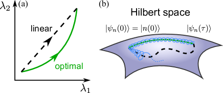
Figure 1: Illustration of the evolution under the linear (black dashed line) and the optimal (green solid curve) protocols. (a) The control protocols with two control parameters $\lambda_{1}$ and $\lambda_{2}$. (b) The evolution of the state $\left|\psi_{n}(t)\right\rangle$. The instantaneous eigenstate $\left|n(t)\right\rangle$ is represented by the black dashed and the green solid curves. In the optimal protocol, the state $\left|\psi_{n}(t)\right\rangle$ deviates from the instantaneous eigenstate $\left|n(t)\right\rangle$ uniformly. While in the linear protocol, the deviation can increase greatly when the overall non-adiabatic transition rate $\tilde{T}_{n}(s)$ becomes large.

We emphasize that the first-order results [Eqs. (5) and (8)] are only valid for slow processes when $P_{n}(t)\ll 1$ is satisfied. In this situation, the state $\left|\psi_{n}(t)\right\rangle$ during the evolution is close to the instantaneous eigenstate $\left|n(t)\right\rangle$. With the shorter operation time, the first-order approximation may fail at a specific time point when the overall non-adiabatic transition rate $\tilde{T}_{n}(s)\coloneqq[\sum_{l\neq n}|\tilde{T}_{nl}(s)|^{2}]^{1/2}$ becomes large. To make the quantum adiabatic condition (1) possibly hold on the whole evolution, the optimal protocol to vary the control parameter is to keep

$$\tilde{T}_{n}(s)=\mathrm{const}.$$ (9)

We illustrate the evolution of the state under the linear and the optimal protocols in Fig. 1. In the linear protocol, the state $\left|\psi_{n}(t)\right\rangle$ deviates from the instantaneous eigenstate $\left|n(t)\right\rangle$ increasingly, and the final state $\left|\psi_{n}(\tau)\right\rangle$ becomes much different from the final instantaneous eigenstate $\left|n(\tau)\right\rangle$. In the optimal protocol, the transition probability $P_{n}(t)$ is regularly oscillated for a few-level system (Sec. III), and becomes uniform for a quantum many-body system (Sec. IV). One can thus properly control the deviation from the instantaneous eigenstate $\left|n(t)\right\rangle$.

To estimate the transition probability, we define the quantum adiabatic length $\mathcal{L}_{n}$ for the $n$-th eigenstate with the overall non-adiabatic transition rate $\tilde{T}_{n}(s)$ as

$$\mathcal{L}_{n}\coloneqq\int_{0}^{1}\tilde{T}_{n}(s)ds.$$ (10)

We consider the variation of the Hamiltonian $H(t)=H[\vec{\lambda}(t)]$ through multiple control parameters $\vec{\lambda}=\{\lambda_{i}\}$. The quantum adiabatic length is determined by the path in the control parameter space

$$\mathcal{L}_{n}=\int_{0}^{1}\sqrt{\sum_{ij}\tilde{\lambda}_{i}^{\prime}(s)g_{n,ij}(\vec{\lambda})\tilde{\lambda}_{j}^{\prime}(s)}ds,$$ (11)

and is independent of the control protocol on the path. We coin the dynamical quantum geometric tensor for the metric

$$g_{n,ij}(\vec{\lambda})=\mathrm{Re}\sum_{l\neq n}\frac{\left\langle l\right|\frac{\partial H}{\partial\lambda_{i}}\left|n\right\rangle\left\langle n\right|\frac{\partial H}{\partial\lambda_{j}}\left|l\right\rangle}{(E_{n}-E_{l})^{4}},$$ (12)

due to its similarity to the quantum geometric tensor (Provost and Vallee, 1980) except that the index in the numerator is $4$ instead of $2$. In the optimal protocol, the transition probability according to Eq. (5) is estimated by

$$P_{n}(t)\approx\frac{2\mathcal{L}_{n}^{2}}{\tau^{2}},$$ (13)

when neglecting the oscillation term. One can further choose the geodesic path connecting $\vec{\lambda}(0)$ and $\vec{\lambda}(\tau)$ to minimize the quantum adiabatic length $\mathcal{L}_{n}$ and reduce the transition probability $P_{n}(t)$. Take into account the oscillation term $\Lambda_{nl}(t)$, the upper bound (8) of the transition probability for the optimal protocol becomes $P_{n,+}(t)=4\mathcal{L}_{n}^{2}/\tau^{2}.$ The quantum adiabatic length $\mathcal{L}_{n}$, with the dimension of time, indicates the timescale of quantum adiabaticity, and the quantum adiabatic condition is geometrically reformulated in Eq. (2).

The proposed dynamical quantum geometric tensor fairly assesses the non-adiabatic transition from $\left|n\right\rangle$ to all the other states. In Ref. (Rezakhani et al., 2009), the used metric for the optimization is an approximation of Eq. (12) by substituting all $E_{n}-E_{l}$ in Eq. (12) with the energy gap between the ground state and the first excited state. With the dynamical quantum geometric tensor, the optimization of the protocol to reach quantum adiabaticity in relatively short time is converted to finding the geodesic path on the control parameter space.

III Landau-Zener Model

We employ the above geometric method to optimize the control for the simplest quantum system, i.e., a two-level system, which also serves as the basic element as a qubit in quantum computation. The precise control of the state of the qubit ensures the reliability of a quantum computer (Albash and Lidar, 2018). We consider the well-known Landau-Zener model (Zener, 1932; Landau, 1932) described by the Hamiltonian

$$H=\frac{\Delta}{2}(\sigma_{x}+\lambda\sigma_{z}),$$ (14)

where $\lambda$ serves as the control parameter, and $\sigma_{x},\sigma_{z}$ are the Pauli matrices. The origin Landau-Zener model adopts a linear protocol to vary the control parameter $\lambda$. The initial state is chosen as the ground state $\left|\psi_{\mathrm{g}}(0)\right\rangle=\left|\mathrm{g}(0)\right\rangle$ with the initial control parameter satisfying $\left|\lambda\right|\gg 1$. For long operation time, the transition probability $P_{\mathrm{g}}=\left|\left\langle\mathrm{e}(\tau)\left|\psi_{\mathrm{g}}(\tau)\right\rangle\right.\right|^{2}$ approaches zero at the end of the evolution.

To derive the optimal protocol, we rewrite the Hamiltonian [Eq. (14)] into

$$H=\frac{\Delta}{2}\sqrt{1+\lambda^{2}}\left(\left|\mathrm{e}\right\rangle\left\langle\mathrm{e}\right|-\left|\mathrm{g}\right\rangle\left\langle\mathrm{g}\right|\right),$$ (15)

with the instantaneous eigenstates

$$\left|\mathrm{g}\right\rangle =\left(\begin{array}[]{c}-\sqrt{\frac{\sqrt{1+\lambda^{2}}-\lambda}{2\sqrt{1+\lambda^{2}}}}\\ \sqrt{\frac{\sqrt{1+\lambda^{2}}+\lambda}{2\sqrt{1+\lambda^{2}}}}\end{array}\right),\;\left|\mathrm{e}\right\rangle=\left(\begin{array}[]{c}\sqrt{\frac{\sqrt{1+\lambda^{2}}+\lambda}{2\sqrt{1+\lambda^{2}}}}\\ \sqrt{\frac{\sqrt{1+\lambda^{2}}-\lambda}{2\sqrt{1+\lambda^{2}}}}\end{array}\right).$$ (20)

According to Eq. (9), the optimal protocol satisfies

$$\frac{[\tilde{\lambda}_{\mathrm{op}}^{\prime}(s)]^{2}}{[1+\tilde{\lambda}_{\mathrm{op}}(s)^{2}]^{3}}=\mathrm{const}.$$ (21)

With the initial and the final values of the control parameter $\tilde{\lambda}(0)=-\lambda_{0}$ and $\tilde{\lambda}(1)=\lambda_{0}$, the optimal protocol is solved as

$$\tilde{\text{$\lambda$}}_{\mathrm{op}}(s)=\frac{-\lambda_{0}(1-2s)}{\sqrt{1+4\lambda_{0}^{2}s(1-s)}},$$ (22)

while the linear protocol is $\tilde{\text{$\lambda$}}_{\mathrm{lin}}(s)=-\lambda_{0}(1-2s)$. For the two-level system, the quantum adiabatic lengths are identical for the ground and the excited states, i.e., $\mathcal{L}_{\mathrm{g}}=\mathcal{L}_{\mathrm{e}}=\left|\lambda_{0}\right|/(\Delta\sqrt{\lambda_{0}^{2}+1})$.

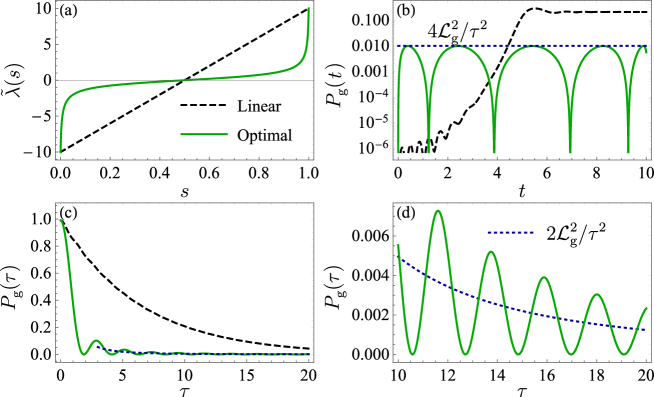
Figure 2: The transition probability for the Landau-Zener model. The parameters are set to be $\lambda_{0}=10$ and $\Delta=2$. (a) The control schemes for the linear and the optimal protocols. (b) The transition probability $P_{\mathrm{g}}(t)$ during the whole evolution with $\tau=10$. The blue dotted line shows the upper bound $P_{\mathrm{g}}(t)\leq 4\mathcal{L}_{\mathrm{g}}^{2}/\tau^{2}$ for the optimal protocol. (c) and (d) The final transition probability $P_{\mathrm{g}}(\tau)$ as a function of the operation time $\tau$. In the optimal protocol, the final transition probability is estimated by $P_{\mathrm{g}}(\tau)\approx 2\mathcal{L}_{\mathrm{g}}^{2}/\tau^{2}$ (blue dotted curve) with $\mathcal{L}_{\mathrm{g}}=0.498$.

Figure 2 shows the numerical results of the transition probability $P_{\mathrm{g}}(\tau)$ for the Landau-Zener model under the linear and the optimal protocols. In Fig. 2(a), we compare the linear protocol $\tilde{\text{$\lambda$}}_{\mathrm{lin}}(s)$ and the optimal protocol $\tilde{\lambda}_{\mathrm{op}}(s)$ with $\lambda_{0}=10$. In the optimal protocol, the control parameter $\lambda$ is varied fast (slowly) with large (small) energy spacing at $s=0$ and $1$ ($s=0.5$). Figure. 2(b) shows the transition probability $P_{\mathrm{g}}(t)$ of the two protocols during the whole evolution with $\tau=10$ and $\Delta=2$. In the linear protocol (black dashed curve), the transition probability $P_{\mathrm{g}}(t)$ keeps increasing before the energy spacing reaches the minimum at $t=\tau/2$. In the optimal protocol (green solid curve), the transition probability $P_{\mathrm{g}}(t)$ increases rapidly at the initial time, but soon saturates the upper bound $4\mathcal{L}_{\mathrm{g}}^{2}/\tau^{2}$ (blue dotted line). We observe the oscillation in the transition probability $P_{\mathrm{g}}(t)$. Its value approaches almost zero at specific moments. Such a phenomenon can be understood from the first-order result Eq. (5). For the two-level system, there is only one term $l=\mathrm{e}$ left in the summation in Eq. (5), and the transition probability $P_{\mathrm{g}}(t)$ can approach zero with a proper value of the phase factor in the oscillation term $\Lambda_{\mathrm{ge}}(t)$. The oscillation phenomenon has also been observed in the quantum harmonic oscillator with the time-dependent frequency (Chen et al., 2019b).

In Fig 2(c) and (d), we compare the final transition probability $P_{\mathrm{g}}(\tau)$ of the two protocols with different operation time $\tau$. In the optimal protocol, the probability $P_{\mathrm{g}}(\tau)$ decreases more rapidly (green curve) with the increase of the operation time, and is estimated by $P_{\mathrm{g}}(t)\approx 2\mathcal{L}_{\mathrm{g}}^{2}/\tau^{2}$ with neglecting the oscillation. The quantum adiabaticity is reached with shorter operation time in the optimal protocol than in the linear protocol.

In Appendix A, we optimize the control of a general two-level system with changing the direction of the control parameters.

IV One-dimensional transverse Ising model

It is intriguing to employ the geometric method to optimize the control of quantum many-body systems. For a system with multiple energy eigenstates, the non-adiabatic transitions to all the other states contribute to the transition probability $P_{n}(t)$, whose behavior can still be investigated from the dynamical quantum geometric tenser. As an illustrative example, we consider the one-dimensional transverse Ising model (Sachdev, 2017). The Hamiltonian reads

$$H=-J\sum_{i=1}^{N}\left(\sigma_{i}^{z}\sigma_{i+1}^{z}+\lambda\sigma_{i}^{x}\right).$$ (23)

We consider the site number $N$ even and periodic boundary condition $\sigma_{N+1}=\sigma_{1}$. The sign of $J$ does not affect the results of the transition probability $P_{n}(t)$, and we set $J=1$ in all the numerical calculation for convenience. This model can be mapped into a free Fermion model described by quasiparticles, and is thus fully solvable. The quantum phase transition of this model occurs at the critical points $\lambda=\pm 1$ (Sachdev, 2017). The external field $\lambda$ serves as the control parameter, the control scheme of which is usually considered as the instant (Quan et al., 2006; Silva, 2008) or the linear quenches (Zurek et al., 2005; Dziarmaga, 2005). For the linear quench across the critical point, the average excitation (del Campo, 2018) and the average excess work (Fei et al., 2020) scale with the operation time as $\tau^{-1/2}$.

For the one-dimensional transverse Ising model in the thermodynamic limit, the quantum phase transition close the energy gap of the system at the critical points, resulting in the divergence of the quantum geometry tensor (Venuti and Zanardi, 2007; Zanardi et al., 2007). The divergence also exists for the dynamical quantum geometric tensor, and prevents constructing an optimal protocol to cross the critical point, but the current method can be used to optimize the control scheme either for a finite-size system or without crossing the critical point.

Under the Jordan-Wigner transformation, the model is mapped to a free Fermion model with the Hamiltonian (Sachdev, 2017)

$$H =\sum_{k>0}H_{k},$$ (24)

where $k$ ranges from $0$ to $\pi-2\pi/N$ with the interval $2\pi/N$. In the $k$-subspace, the Hamiltonian entangles the modes $k$ and $-k$ as

$$H_{k}=2J\psi_{k}^{\dagger}\left(\begin{array}[]{cc}\lambda-\cos k&-i\sin k\\ i\sin k&-\lambda+\cos k\end{array}\right)\psi_{k},$$ (25)

in terms of $\psi_{k}^{\dagger}=\left(\begin{array}[]{cc}c_{k}^{\dagger}&c_{-k}\end{array}\right)$. For the mode $k=0$ or $\pi$, the evolution can be also described by Eq. (25) with $\psi_{0}^{\dagger}=\left(\begin{array}[]{cc}c_{0}^{\dagger}&c_{\pi}\end{array}\right)$, and the two modes do not mix since the off-diagonal terms are zero. The Hamiltonian is diagonalized under the Bogliubov transformation as

$$H_{k}=\epsilon_{k}(A_{k}^{\dagger}A_{k}-\frac{1}{2}).$$ (26)

The energy and the annihilation operator of the quasiparticle are $\epsilon_{k}=2J\left(\lambda^{2}-2\lambda\cos k+1\right)^{1/2}$ and $A_{k}=u_{k}c_{k}-iv_{k}c_{-k}^{\dagger}$, where the coefficients are $u_{k}=\cos(\theta_{k}/2)$ and $v_{k}=\sin(\theta_{k}/2)$ with $\tan\theta_{k}=\sin k/(\lambda-\cos k)$.

For the initial ground state, the wave-function between different pairs $\pm k$ are in the direct product form. We write down the ground-state wave-function in each $k$-subspace as

$$\left|\mathrm{g}(k)\right\rangle=u_{k}\left|0_{k}0_{-k}\right\rangle+iv_{k}\left|1_{k}1_{-k}\right\rangle,$$ (27)

where $\left|l_{k}\right\rangle$ is the Fock state satisfying $c_{k}^{\dagger}c_{k}\left|l_{k}\right\rangle=l_{k}\left|l_{k}\right\rangle$ with $l=\pm 1$. The single-occupy states are always the eigenstates $H_{k}\left|0_{k}1_{-k}\right\rangle=0,$ $H_{k}\left|1_{k}0_{-k}\right\rangle=0$ of the Hamiltonian $H_{k}$. The finite-time variation does not induce the non-adiabatic transition to these states. Therefore, the Hamiltonian in each $k$-subspace is equivalent to that of a two-level system. The non-adiabatic transitions are obtained with several pairs of states $\left|0_{k}0_{-k}\right\rangle$ and $\left|1_{k}1_{-k}\right\rangle$.

We employ the geometric method to optimize the control scheme of the quench for the one-dimensional transverse Ising model with finite site number $N$. Our task is to find the optimal protocol to vary the external field $\lambda$. As shown in Appendix B, the quantum adiabatic length is obtained as

$$d\mathcal{L}_{\mathrm{g}}=\sum_{k>0}\frac{\sin k}{8J\left(\lambda^{2}-2\lambda\cos k+1\right)^{3/2}}d\lambda,$$ (28)

where the summation of $k$ is limited to $k=2\pi/N,4\pi/N,...\pi-2\pi/N$. The optimal protocol $\tilde{\lambda}_{\mathrm{op}}(s)$ follows as

$$[\tilde{\lambda}_{\mathrm{op}}^{\prime}(s)]^{2}\sum_{k>0}\frac{\sin^{2}k}{\left[\tilde{\lambda}_{\mathrm{op}}(s)^{2}-2\tilde{\lambda}_{\mathrm{op}}(s)\cos k+1\right]^{3}}=\mathrm{const}.$$ (29)

Due to the quasiparticle representation of this model, the transition probability $P_{\mathrm{g}}(t)$ of the ground state of this many-body system is the product of the transition probabilities of the two-level system in each $k$-subspace.

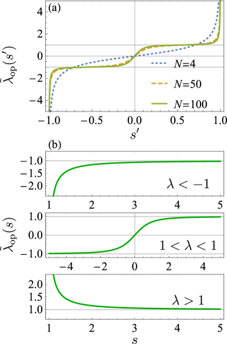
Figure 3: The optimal protocol for the one-dimensional transverse Ising model. (a) The optimal protocols for finite site numbers $N=4,50,100$ with the time $s^{\prime}$ rescaled to $(-1,1)$. (b) The optimal protocol in the thermodynamic limit $N\rightarrow\infty$. We show the the optimal protocols Eq. (31) for the three regions $\lambda<-1$, $-1<\lambda<1$ and $\lambda>1$. The metric is divergent at the critical points $\lambda=\pm 1$ (horizontal gray line), which cannot be crossed in finite time.

For given site number $N$, the optimal protocol can be numerically solved by Eq. (29). For $N=4$, only one term with $k=\pi/2$ leaves in the summation, and the optimal protocol $\tilde{\lambda}_{\mathrm{op}}(s^{\prime})=s^{\prime}/\sqrt{1-s^{\prime 2}}$ coincides with that of the Landau-Zener model with a rescaled time $s^{\prime}\in(-1,1)$. In Fig. 3 (a), the optimal protocols are shown for different site numbers $N=4,50,100$. With the increase of the site number $N$, it consumes more operation time to cross the critical points $\lambda=\pm 1$.

In the thermodynamic limit $N\rightarrow\infty$, Eq. (29) is simplified into

$$\frac{\tilde{\lambda}_{\mathrm{op}}^{\prime}(s)^{2}}{\left|\tilde{\lambda}_{\mathrm{op}}(s)^{2}-1\right|^{3}}=\mathrm{const},$$ (30)

and the optimal protocol is explicitly obtained as

$$\tilde{\lambda}_{\mathrm{op}}(s)=\begin{cases}\frac{-s}{\sqrt{s^{2}-1}}&\lambda<-1\\ \frac{s}{\sqrt{1+s^{2}}}&-1<\lambda<1\\ \frac{s}{\sqrt{s^{2}-1}}&\lambda>1,\end{cases}$$ (31)

as shown in Fig. 3(b). The constant has been absorbed into the rescaled time $s$ here. In the three regions $\lambda<-1$, $-1<\lambda<1$ and $\lambda>1$ of the control parameter, the ranges of the rescaled time are $s\in(1,+\infty)$, $(-\infty,+\infty)$ and $(1,+\infty)$, respectively. Equation (31) shows that in the thermodynamic limit $N\rightarrow\infty$ the optimal protocol cannot cross the critical points $\lambda=\pm 1$ in any finite time process.

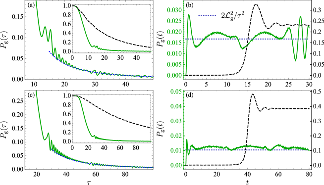
Figure 4: The transition probability for the one-dimensional transverse Ising model. The site number is $N=50$ in (a), (b) and $N=100$ in (c), (d) with $J=1$. The external field is varied from $\tilde{\lambda}(0)=2$ to $\tilde{\lambda}(1)=0$ via the optimal protocol $\tilde{\lambda}_{\mathrm{op}}(s)$ (green solid curve) and the linear protocol $\tilde{\lambda}_{\mathrm{lin}}(s)=2(1-s)$ (black dashed curve). All the blue dashed curves show the estimation $2\mathcal{L}_{\mathrm{g}}^{2}/\tau^{2}$. (a) and (c) The final transition probability $P_{\mathrm{g}}(\tau)$ as a function of the operation time $\tau$. The results of the linear protocol are shown in the insets. (b) and (d) The transition probability $P_{\mathrm{g}}(t)$ during the whole evolution. The values of $P_{\mathrm{g}}(t)$ in the linear protocol are multiplied ten times.

Figure 4 shows the numerical results of the transition probability $P_{\mathrm{g}}(\tau)$ with the linear protocol $\tilde{\lambda}_{\mathrm{lin}}(s)=\tilde{\lambda}(0)(1-s)+\tilde{\lambda}(1)s$ and the optimal protocol $\tilde{\lambda}_{\mathrm{op}}(s)$ [Eq. (29)] for the one-dimensional transverse Ising model. The initial and the final values of the control parameter are $\tilde{\lambda}(0)=2$ and $\tilde{\lambda}(1)=0$. The site number is $N=50$ in (a), (b) and $N=100$ in (c), (d). The transition probability of the ground state is obtained by numerically solving the time-dependent Schrödinger equation with $J=1$. Figure 4(a) and (c) present the final transition probability $P_{\mathrm{g}}(\tau)$ as a function of the operation time $\tau$. The final transition probability in the optimal protocol is well estimated by $P_{\mathrm{g}}(\tau)\approx 2\mathcal{L}_{\mathrm{g}}^{2}/\tau^{2}$ (blue dotted curve), and is much smaller than that in the linear protocol as shown by the insets. With more spins in the system, it requires a longer operation time to remain the same transition probability to cross the critical point $\lambda=1$. The phenomenon is induced by the modes around $k\simeq 0$ with slower dynamics (del Campo, 2018).

Figure 4(b) and (d) present the transition probability $P_{\mathrm{g}}(t)$ during the whole evolution with given operation time $\tau=30$ and $\tau=80$, respectively. In the linear protocol, the transition probability $P_{\mathrm{g}}(t)$ increase rapidly at the moment $t/\tau=0.5$ across the critical point. In the optimal protocol, the transition probability during the whole evolution is well estimated by $P_{\mathrm{g}}(t)\approx 2\mathcal{L}_{\mathrm{g}}^{2}/\tau^{2}$ (blue dotted line). The oscillation in $P_{\mathrm{g}}(t)$ is much weaker but more irregular compared to the case of the two-level system, since $P_{\mathrm{g}}(t)$ is the product of the transition probabilities in each $k$-subspace.

V Conclusion

We proposed the dynamical quantum geometric tensor to speed up finite-time adiabatic processes. The dynamical quantum geometric tensor is a metric in the control parameter space. The length induced by metric, i.e., the quantum adiabatic length, determines the timescale of quantum adiabaticity. The optimal protocol is to vary the control parameter with a constant velocity along the geodesic path according to the metric, and the transition probability is estimated (bounded) by the quantum adiabatic length as $P_{n}\approx 2\mathcal{L}_{n}^{2}/\tau^{2}$ ($P_{n}\leq 4\mathcal{L}_{n}^{2}/\tau^{2}$). We employ the geometric method to optimize the control of the Landau-Zener model and the one-dimensional transverse Ising model, and verify the transition probability in the optimal protocol is much smaller than that in the linear protocol with given operation time.

Appendix A General two-level system

For a two-level system, the Hamiltonian is generally written as

$$H=\frac{1}{2}(\lambda_{x}\sigma_{x}+\lambda_{y}\sigma_{y}+\lambda_{z}\sigma_{z}),$$ (32)

with the control parameters $\vec{\lambda}=(\lambda_{x},\lambda_{y},\lambda_{z})$. According to Eq. (12), the dynamical quantum geometric tensor is obtained as

$$g_{\mathrm{g}}(\vec{\lambda})=\frac{1}{4\lambda^{6}}\left(\begin{array}[]{ccc}\lambda_{y}^{2}+\lambda_{z}^{2}&-\lambda_{x}\lambda_{y}&-\lambda_{x}\lambda_{z}\\ -\lambda_{x}\lambda_{y}&\lambda_{x}^{2}+\lambda_{z}^{2}&-\lambda_{y}\lambda_{z}\\ -\lambda_{x}\lambda_{z}&-\lambda_{y}\lambda_{z}&\lambda_{x}^{2}+\lambda_{y}^{2}\end{array}\right),$$ (33)

with $\lambda=\sqrt{\lambda_{x}^{2}+\lambda_{y}^{2}+\lambda_{z}^{2}}$. For the two-level system, the metric for the excited state is the same $g_{\mathrm{e}}(\vec{\lambda})=g_{\mathrm{g}}(\vec{\lambda})$. Under the sphere coordinates $(\lambda,\theta,\phi)$ with $\cos\theta=\lambda_{z}/\lambda$ and $\tan\phi=\lambda_{y}/\lambda_{x}$, the quantum adiabatic length is simplified into

$$d\mathcal{L}_{\mathrm{g}}^{2}=\frac{\sin^{2}\theta d\theta^{2}+d\phi^{2}}{4\lambda^{2}}.$$ (34)

The metric is degenerate along the direction $\vec{\lambda}/\lambda$, since the changing strength with fixed direction does not generate the transition between different eigenstates. We constrain the control of the parameters on a sphere $\lambda=\mathrm{const}$. The geodesic paths on the sphere are large circles.

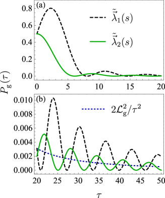
Figure 5: The final transition probability $P_{\mathrm{g}}(\tau)$ for the control of the external field $\vec{\lambda}$ constraint on the sphere $\lambda=1$. Two protocols are considered, the small-circle protocol $\tilde{\vec{\lambda}}_{1}(s)$ and the large-circle protocol $\tilde{\vec{\lambda}}_{2}(s)$. (a) The results with short operation time $\tau\in(0,20]$. (b) The results with longer operation time $\tau\in[20,50]$. The blue dotted curve shows the estimation $P_{\mathrm{g}}(\tau)\approx 2\mathcal{L}_{\mathrm{g}}^{2}/\tau^{2}$ with the length $\mathcal{L}_{\mathrm{g}}=\pi/4$ of the path on the large circle.

We next compare different control protocols to vary the external field constraint on the sphere $\lambda=1$. Two protocols are adopted to vary the external field from the initial point $\tilde{\vec{\lambda}}(0)=(1/\sqrt{2},0,1/\sqrt{2})$ to the final point $\tilde{\vec{\lambda}}(1)=(-1/\sqrt{2},0,1/\sqrt{2})$, with one on a small circle

$$\tilde{\vec{\lambda}}_{1}(s)=\frac{\sqrt{2}}{2}(\cos(\pi s),\sin(\pi s),1),$$ (35)

and the other on a large circle (geodesic path)

$$\tilde{\vec{\lambda}}_{2}(s)=(\sin[\frac{\pi}{4}(1-2s)],0,\cos[\frac{\pi}{4}(1-2s)]).$$ (36)

According to Eq. (34), the quantum adiabatic lengths of the two paths are $\mathcal{L}_{\mathrm{g}}=\sqrt{2}\pi/4$ and $\pi/4$. In Figure 5, we show the transition probability $P_{\mathrm{g}}(\tau)$ for the two protocols with different operation time $\tau$. The transition probability $P_{\mathrm{g}}(\tau)$ of the protocol on the geodesic path is smaller. In both protocols, $P_{\mathrm{g}}(\tau)$ can be estimated by $P_{\mathrm{g}}(\tau)\approx 2\mathcal{L}_{\mathrm{g}}^{2}/\tau^{2}$ when neglecting the oscillation. In Fig. 5(b), the estimation of the quantum adiabatic length is shown for the second protocol by the blue dotted curve.

Appendix B Optimal protocol of the one-dimensional transverse Ising model

For the one-dimensional transverse Ising model, we represent the instantaneous eigenstates of the many-body system as the tensor product $\left|\Psi_{\{n(k)\}}\right\rangle=\underset{k>0}{\bigotimes}\left|n(k)\right\rangle$, where $\left|n(k)\right\rangle$ is the eigenstate in each subspace, and $n=\mathrm{g}$ and $\mathrm{e}$ represents the ground state and the excited state, respectively. Here, we do not consider the modes $k\neq 0,\pi$, since the eigenstates of them remain unchanged when varying the control parameter. The quantum adiabatic length $\mathcal{L}_{\{n(k)\}}$ of the eigenstate $\left|\Psi_{\{n(k)\}}\right\rangle$ is determined by Eq. (10) as

$$d\mathcal{L}_{\{n(k)\}}=\left|d\lambda\right|\left[\sum_{\{l(k)\}\neq\{n(k)\}}\left|\frac{\left\langle\Psi_{\{l(k)\}}\right|\frac{\partial}{\partial\lambda}\left|\Psi_{\{n(k)\}}\right\rangle}{\tilde{E}_{\{n(k)\}}(s)-\tilde{E}_{\{l(k)\}}(s)}\right|^{2}\right]^{1/2},$$ (37)

where $\{n(k)\}$ and $\{l(k)\}$ are the eigenstates of the many-body system with $n,l=\mathrm{g}$ or $\mathrm{e}$. The change of the many-body eigenstate is

$$\frac{\partial}{\partial\lambda}\left|\Psi_{\{n(k)\}}\right\rangle=\sum_{k^{\prime}>0}\frac{\partial\left|n(k^{\prime})\right\rangle}{\partial\lambda}\otimes\underset{k\neq k^{\prime}}{\bigotimes}\left|n(k)\right\rangle.$$ (38)

Therefore, non-zero product $\left\langle\Psi_{\{l(k)\}}\right|\partial_{\lambda}\left|\Psi_{\{n(k)\}}\right\rangle$ requires that the set $\{l(k)\}$ has only one element different from $\{n(k)\}$. We write this different element as $n(k^{\prime})$ in $\{n(k)\}$ and $\bar{n}(k^{\prime})$ in $\{l(k)\}$, where $\bar{n}$ is the opposite state of $n$. The non-adiabatic transition rate is simplified as

$$\frac{\left\langle\Psi_{\{l(k)\}}\right|\frac{\partial}{\partial\lambda}\left|\Psi_{\{n(k)\}}\right\rangle}{\tilde{E}_{\{n(k)\}}(s)-\tilde{E}_{\{l(k)\}}(s)}=\frac{\left\langle\bar{n}(k^{\prime})\right|\frac{\partial}{\partial\lambda}\left|n(k^{\prime})\right\rangle}{\epsilon_{n(k^{\prime})}-\epsilon_{\bar{n}(k^{\prime})}}.$$ (39)

The summation over $\{l(k)\}$ gives $N/2$ non-zero terms

$$\sum_{\{l(k)\}\neq\{n(k)\}}\left|\frac{\left\langle\Psi_{\{l(k)\}}\right|\frac{\partial}{\partial\lambda}\left|\Psi_{\{n(k)\}}\right\rangle}{\tilde{E}_{\{n(k)\}}(s)-\tilde{E}_{\{l(k)\}}(s)}\right|^{2}=\sum_{k^{\prime}>0}\left|\frac{\left\langle\bar{n}(k^{\prime})\right|\frac{\partial}{\partial\lambda}\left|n(k^{\prime})\right\rangle}{\epsilon_{n(k^{\prime})}-\epsilon_{\bar{n}(k^{\prime})}}\right|.$$ (40)

The same result is obtained for both $n=\mathrm{g}$ and $\mathrm{e}$

$$\left|\frac{\left\langle\bar{n}(k^{\prime})\right|\frac{\partial}{\partial\lambda}\left|n(k^{\prime})\right\rangle}{\epsilon_{n(k^{\prime})}-\epsilon_{\bar{n}(k^{\prime})}}\right|^{2}=\frac{\sin^{2}k^{\prime}}{64J^{2}\left(\lambda^{2}-2\lambda\cos k^{\prime}+1\right)^{3}}.$$ (41)

The optimal protocol Eq. (29) is obtained by varying the control parameter $\lambda$ with the constant velocity of the quantum adiabatic length.

References

- Peirce et al. (1988) A. P. Peirce, M. A. Dahleh, and H. Rabitz, Phys. Rev. A 37, 4950 (1988).
- Caneva et al. (2009) T. Caneva, M. Murphy, T. Calarco, R. Fazio, S. Montangero, V. Giovannetti, and G. E. Santoro, Phys. Rev. Lett. 103, 240501 (2009).
- Bason et al. (2011) M. G. Bason, M. Viteau, N. Malossi, P. Huillery, E. Arimondo, D. Ciampini, R. Fazio, V. Giovannetti, R. Mannella, and O. Morsch, Nat. Phys. 8, 147 (2011).
- Brif et al. (2014) C. Brif, M. D. Grace, M. Sarovar, and K. C. Young, New J. Phys. 16, 065013 (2014).
- Santos and Sarandy (2015) A. C. Santos and M. S. Sarandy, Sci. Rep. 5, 15775 (2015).
- Machnes et al. (2018) S. Machnes, E. Assémat, D. Tannor, and F. K. Wilhelm, Phys. Rev. Lett. 120, 150401 (2018).
- Zulkowski and DeWeese (2015) P. R. Zulkowski and M. R. DeWeese, Phys. Rev. E 92, 032113 (2015).
- Solon and Horowitz (2018) A. P. Solon and J. M. Horowitz, Phys. Rev. Lett. 120, 180605 (2018).
- Cavina et al. (2018) V. Cavina, A. Mari, A. Carlini, and V. Giovannetti, Phys. Rev. A 98, 052125 (2018).
- Scandi and Perarnau-Llobet (2019) M. Scandi and M. Perarnau-Llobet, Quantum 3, 197 (2019).
- Vu and Saito (2022) T. V. Vu and K. Saito, Phys. Rev. Lett. 128, 010602 (2022).
- Farhi et al. (2001) E. Farhi, J. Goldstone, S. Gutmann, J. Lapan, A. Lundgren, and D. Preda, Science 292, 472 (2001).
- Sarandy and Lidar (2005) M. S. Sarandy and D. A. Lidar, Phys. Rev. Lett. 95, 250503 (2005).
- Nielsen (2006) M. A. Nielsen, Science 311, 1133 (2006).
- Menicucci et al. (2006) N. C. Menicucci, P. van Loock, M. Gu, C. Weedbrook, T. C. Ralph, and M. A. Nielsen, Phys. Rev. Lett. 97, 110501 (2006).
- Aharonov et al. (2007) D. Aharonov, W. van Dam, J. Kempe, Z. Landau, S. Lloyd, and O. Regev, SIAM J. Comput. 37, 166 (2007).
- Albash and Lidar (2018) T. Albash and D. A. Lidar, Rev. Mod. Phys. 90, 015002 (2018).
- Feldmann and Kosloff (2000) T. Feldmann and R. Kosloff, Phys. Rev. E 61, 4774 (2000).
- Kieu (2004) T. D. Kieu, Phys. Rev. Lett. 93, 140403 (2004).
- Quan et al. (2007) H. T. Quan, Y. X. Liu, C. P. Sun, and F. Nori, Phys. Rev. E 76, 031105 (2007).
- Quan (2009) H. T. Quan, Phys. Rev. E 79, 041129 (2009).
- Plastina et al. (2014) F. Plastina, A. Alecce, T. Apollaro, G. Falcone, G. Francica, F. Galve, N. L. Gullo, and R. Zambrini, Phys. Rev. Lett. 113, 260601 (2014).
- Amin (2009) M. H. S. Amin, Phys. Rev. Lett. 102, 220401 (2009).
- Sakurai (2011) J. J. Sakurai, Modern Quantum Mechanics (Addison-Wesley, Boston, 2011).
- Shevchenko et al. (2010) S. Shevchenko, S. Ashhab, and F. Nori, Phys. Rep. 492, 1 (2010).
- Demirplak and Rice (2003) M. Demirplak and S. A. Rice, J. Phys. Chem. A 107, 9937 (2003).
- Demirplak and Rice (2005) M. Demirplak and S. A. Rice, J. Phys. Chem. B 109, 6838 (2005).
- Masuda and Nakamura (2008) S. Masuda and K. Nakamura, Phys. Rev. A 78, 062108 (2008).
- Berry (2009) M. V. Berry, J. Phys. A: Math. Theor. 42, 365303 (2009).
- Chen et al. (2010) X. Chen, A. Ruschhaupt, S. Schmidt, A. del Campo, D. Guéry-Odelin, and J. G. Muga, Phys. Rev. Lett. 104, 063002 (2010).
- del Campo (2013) A. del Campo, Phys. Rev. Lett. 111, 100502 (2013).
- Santos and Sarandy (2017) A. C. Santos and M. S. Sarandy, J. Phys. A: Math. Theor. 51, 025301 (2017).
- Guéry-Odelin et al. (2019) D. Guéry-Odelin, A. Ruschhaupt, A. Kiely, E. Torrontegui, S. Martínez-Garaot, and J. Muga, Rev. Mod. Phys. 91, 045001 (2019).
- Hu et al. (2018) C.-K. Hu, J.-M. Cui, A. C. Santos, Y.-F. Huang, M. S. Sarandy, C.-F. Li, and G.-C. Guo, Opt. Lett. 43, 3136 (2018).
- Martínez-Garaot et al. (2015) S. Martínez-Garaot, A. Ruschhaupt, J. Gillet, T. Busch, and J. G. Muga, Phys. Rev. A 92, 043406 (2015).
- Chung et al. (2017) H.-C. Chung, K.-S. Lee, and S.-Y. Tseng, Opt. Express 25, 13626 (2017).
- Martínez-Garaot et al. (2017) S. Martínez-Garaot, J. G. Muga, and S.-Y. Tseng, Opt. Express 25, 159 (2017).
- Liu and Tseng (2017) Y.-H. Liu and S.-Y. Tseng, J. Phys. B: At., Mol. Opt. Phys. 50, 205501 (2017).
- Sun (1988) C.-P. Sun, J. Phys. A: Math. Gen. 21, 1595 (1988).
- Rigolin et al. (2008) G. Rigolin, G. Ortiz, and V. H. Ponce, Phys. Rev. A 78, 052508 (2008).
- Chen et al. (2019a) J.-F. Chen, C.-P. Sun, and H. Dong, Phys. Rev. E 100, 062140 (2019a).
- Chen et al. (2019b) J.-F. Chen, C.-P. Sun, and H. Dong, Phys. Rev. E 100, 032144 (2019b).
- Provost and Vallee (1980) J. P. Provost and G. Vallee, Commun. Math. Phys. 76, 289 (1980).
- Bengtsson (2006) I. Bengtsson, Geometry of quantum states : an introduction to quantum entanglement (Cambridge University Press, Cambridge New York, 2006).
- Zanardi et al. (2007) P. Zanardi, P. Giorda, and M. Cozzini, Phys. Rev. Lett. 99, 100603 (2007).
- Venuti and Zanardi (2007) L. C. Venuti and P. Zanardi, Phys. Rev. Lett. 99, 095701 (2007).
- Rezakhani et al. (2009) A. T. Rezakhani, W.-J. Kuo, A. Hamma, D. A. Lidar, and P. Zanardi, Phys. Rev. Lett. 103, 080502 (2009).
- Rezakhani et al. (2010) A. T. Rezakhani, D. F. Abasto, D. A. Lidar, and P. Zanardi, Phys. Rev. A 82, 012321 (2010).
- Deng et al. (2015) S.-J. Deng, P.-P. Diao, Q.-L. Yu, and H.-B. Wu, Chin. Phys. Lett. 32, 053401 (2015).
- Deng et al. (2018) S. Deng, A. Chenu, P. Diao, F. Li, S. Yu, I. Coulamy, A. del Campo, and H. Wu, Sci. Adv. 4, eaar5909 (2018).
- Zener (1932) C. Zener, Proc. R. Soc. London, Ser. A 137, 696 (1932).
- Landau (1932) L. Landau, Phys. Z. Sowjetunion 2, 46 (1932).
- Mullen et al. (1989) K. Mullen, E. Ben-Jacob, Y. Gefen, and Z. Schuss, Phys. Rev. Lett. 62, 2543 (1989).
- Yan and Wu (2010) Y. Yan and B. Wu, Phys. Rev. A 81, 022126 (2010).
- Zurek et al. (2005) W. H. Zurek, U. Dorner, and P. Zoller, Phys. Rev. Lett. 95, 105701 (2005).
- Dziarmaga (2005) J. Dziarmaga, Phys. Rev. Lett. 95, 245701 (2005).
- Quan et al. (2006) H. T. Quan, Z. Song, X. F. Liu, P. Zanardi, and C. P. Sun, Phys. Rev. Lett. 96, 140604 (2006).
- Silva (2008) A. Silva, Phys. Rev. Lett. 101, 120603 (2008).
- Sachdev (2017) S. Sachdev, Quantum Phase Transitions (Cambridge University Press, 2017).
- del Campo (2018) A. del Campo, Phys. Rev. Lett. 121, 200601 (2018).
- Fei et al. (2020) Z. Fei, N. Freitas, V. Cavina, H. Quan, and M. Esposito, Phys. Rev. Lett. 124, 170603 (2020).
- Zhang and Quan (2022) F. Zhang and H. T. Quan, Phys. Rev. E 105, 024101 (2022).