On the Construction of Distribution-Free Prediction Intervals for an Image Regression Problem in Semiconductor Manufacturing

Abstract

The high-volume manufacturing of the next generation of semiconductor devices requires advances in measurement signal analysis. Many in the semiconductor manufacturing community have reservations about the adoption of deep learning; they instead prefer other model-based approaches for some image regression problems, and according to the 2021 IEEE International Roadmap for Devices and Systems (IRDS) report on Metrology a SEMI standardization committee may endorse this philosophy. The semiconductor manufacturing community does, however, communicate a need for state-of-the-art statistical analyses to reduce measurement uncertainty. Prediction intervals which characterize the reliability of the predictive performance of regression models can impact decisions, build trust in machine learning, and be applied to other regression models. However, we are not aware of effective and sufficiently simple distribution-free approaches that offer valid coverage for important classes of image data, so we consider the distribution-free conformal prediction and conformalized quantile regression framework. The image regression problem that is the focus of this paper pertains to line edge roughness (LER) estimation from noisy scanning electron microscopy images. LER affects semiconductor device performance and reliability as well as the yield of the manufacturing process; the 2021 IRDS emphasizes the crucial importance of LER by devoting a white paper to it in addition to mentioning or discussing it in the reports of multiple international focus teams. It is not immediately apparent how to effectively use normalized conformal prediction and quantile regression for LER estimation. The modeling techniques we apply appear to be novel for finding distribution-free prediction intervals for image data and will be presented at the 2022 SEMI Advanced Semiconductor Manufacturing Conference.

*Inimfon Akpabio, nini16@tamu.edu; Serap Savari, savari@tamu.edu

1 Introduction

The members of the semiconductor manufacturing community have enabled today’s technology. They are the unsung heroes of the machine learning revolution, and they will impact the future of computing. Their work is complex, and we mention only one aspect of it here. There is a lengthy and intricate process to fabricate integrated circuits on the surface of a silicon crystal wafer. That process requires hundreds of inspection and measurement steps [1], and metrology is the “science of measurement, embracing both experimental and theoretical determinations at any level of uncertainty in any field of science and technology” [2, p. 1]. The semiconductor industry has the most stringent metrology requirements in the entire manufacturing sector [2, p. xii] because the billions of devices in a chip must all operate to a tight specification [3]. Much of the measurement data is in the form of digital images, and there is a continual need to improve the process information from microscopy techniques and measurements as technology evolves [4, §5.3]. More generally, the future of semiconductor device fabrication will have growing needs for data processing, information extraction, and knowledge management [4, 5, 6]. Therefore, machine learning may be able to address some of these needs, and an April 2021 McKinsey & Company article attempts to persuade semiconductor-device makers to better capture the significant value-creation potential of artificial intelligence [7]. Yet in semiconductor metrology, “the promise of advanced data analytics (in all its variants) has not been realized” [4, §9]. The Call for Abstracts for this year’s SEMI Advanced Semiconductor Manufacturing Conference (ASMC 2022) lists the “pros and cons of machine learning in measurement signal analysis” [8] as a topic of interest. So what are some of the fundamental issues?

Human factors are affecting the digital transformation of semiconductor manufacturing and other industries [9, 10]. Regarding machine learning, there is another widespread problem. In December 2020 the National Science Foundation and the National Institute of Standards and Technology hosted a gathering of many leaders throughout the manufacturing sector to consider the acceleration of the implementation of artificial intelligence in manufacturing. The complaints of real and perceived risks and a lack of transparency are two of the obstacles to the wider adoption of artificial intelligence [11, 12], and in a different discipline there have been concerns expressed about it in connection with magnetic resonance imaging[13]. Moreover, within semiconductor manufacturing the desire to better understand the uncertainties associated with prediction engines extends beyond machine learning models. Section 5.8.4.2 of the 2021 IEEE International Roadmap for Devices and Systems (IRDS) report on Factory Integration solicits the incorporation of indications of the quality of predictions in its prediction vision [5]. Section 4.2.10 of the 2021 IRDS Executive Summary seeks state-of-the-art statistical analyses to assist in decreasing the measurement uncertainty of sub-7 nm process control [14].

One way to address these issues is through uncertainty quantification (see, e.g., References 15 and 16), and a relatively simple approach is the use of prediction intervals which characterize the reliability of predictive performance. For a regression model outputting a single number a prediction interval offers a range of values in which the output variable lies with high probability. The design of prediction intervals has been extensively studied and has certain objectives. First, the underlying modeling assumptions should be well-suited to the application in order to provide valid coverage. Second, they should produce the shortest possible intervals to help decision makers. Finally, they need an appropriate computational complexity [5, p. 41].

Conformal prediction [17, 18, 19] is a simple, mathematically rigorous, and distribution-free guideline to design prediction intervals; one new variant [20, 21] combines it with a widely used technique known as quantile regression [22]. This framework assumes the exchangeability of data, which roughly means that the examples are representative and their ordering does not matter. In a recent publication[23] we introduced the nanofabrication community to conformal prediction and considered the image regression problem of line edge roughness (LER) estimation; LER is important enough in semiconductor manufacturing to warrant a 2021 IRDS white paper [24]. While quantile regression and conformal prediction are widely used for the construction of prediction intervals, it is not apparent how to effectively apply them to image data, and because of the high dimensionality of image data this question appears to be related to the topic of meta-learning [25] for this application. While our focus is on an LER estimation problem, it may also be interesting to construct prediction intervals for some medical imaging problems such as skeletal bone age assessment from X-ray images [26]. In this paper we present for a data analytics audience the work of an upcoming conference paper [27] (see also Ref. 28) together with some background material. In Section 2, we provide more information about the topic of LER. In Section 3, we briefly review conformal prediction and quantile regression. In Section 4, we discuss the deep convolutional neural network EDGENet [29, 30], which is the image regression model we study. In Section 5, we discuss the new neural networks we introduce to assist with the construction of prediction intervals; these are founded on denoising and successes from image recognition. In Section 6, we provide experimental results. In Section 7, we conclude the paper.

2 Background on LER

For many years, the semiconductor manufacturing industry mainly relied upon photolithography or optical lithography to fabricate multiple integrated circuits on silicon wafers. Here, an image is formed when a thin-film material is selectively exposed to light at 193 nm wavelength [31]. The newer optical technology extreme ultraviolet (EUV) lithography is now in use for the most advanced resolution requirements. In older technologies with larger feature sizes, a mean field theory approximation is adequate to model the effects of the exposure process [32]. However, as feature sizes shrink this approximation no longer suffices to capture the randomness inherent in the lithographic process, and this randomness partially manifests itself as roughness or fluctuations in the edges and widths of features. This roughness has not been scaling at the same rate as feature sizes. This form of uncertainty is increasingly important in linewidth control and is impacting the ultimate limits of resolution in semiconductor lithography [32]. The newer EUV technology uses light at 13.5 nm wavelength to produce smaller circuit features, but statistical fluctuations are growing more important as dimensions shrink [14, §2.2.9].

In order for integrated circuit manufacturing to be economically viable, the yield or the fraction of the produced product with adequate quality must be adequate. To avoid adverse consequences to delay and yield, it is necessary for entire transistors to have uniform characteristics, so it is necessary to estimate and manage random variations on transistor performance including LER [33, pp. 12-14]. LER refers to the edge displacements of a feature edge from a mean edge position and is known to be a crucial factor in the yield of integrated circuit manufacturing (see, e.g., [34, pp. 82-92]). Nanostructure geometry reconstruction algorithms generally require edge-contour extraction algorithms whose performances depend on imaging technologies.

The critical-dimension scanning electron microscope (CD-SEM) is the standard metrology tool to obtain measurements to analyze LER [2, pp. 109, 114]. Here, a focused beam of electrons scans and interacts with the surface of a sample to produce an image of the sample at sub-micron resolutions which contain information about the sample surface geometry. The image quality depends on the energy of the electron beam or the dose provided. High-dose CD-SEM images cause sample damage during repeated measurements [2, p. 42] and have higher acquisition times. Low-dose CD-SEM images have more artifacts in the form of noise, blur, edge effects and other instrument errors which hinder accurate estimation, but they are desirable for manufacturing since they reduce sample damage and acquisition time (see, e.g., Ref. 35). Moreover, the near-term “grand challenges” the 2021 IRDS Executive Summary specifies for yield enhancement include [14, §4.1.11.1]

• “Existing techniques trade off throughput for sensitivity, but at expected defect levels, both throughput and sensitivity are necessary for statistical validity.”

• “Reduction of inspection costs and increase of throughput is crucial in view of cost of ownership.”

• “Detection of line roughness due to process variation.”

• “Reduction of background noise from detection units and samples to improve the sensitivity of systems.”

• “Improvement of signal to noise ratio to delineate defect from process variation.”

• “Where does process variation stop and defect start?”

Since deep learning [36] has altered the practices of signal, image, and video processing, its rapid advances may offer the potential to better address these issues, particularly since line and contour measurements currently require an average of multiple lines or contours in order to sufficiently improve precision (see, e.g., [2, §10.6] and [4, p. 11]). There are some efforts in the industry to use deep learning for defect and fault detection in the fabrication process. Nevertheless, the semiconductor metrology community began to handle these types of problems long before the advent of deep learning, and model-based metrology is respected [4, p. 11]. Yet any model is limited by its assumptions. According to [4, §5.4.1], a SEMI Standards Committee is updating the determination of LER estimation to incorporate a specific model-based methodology. That section of the document states:

“Another important factor in measurement of … LER on imaging tools is edge detection noise. … A methodology has been demonstrated to remove this noise term, leading to an unbiased estimation of the roughness. Use of this is deemed very important to ensuring accuracy of roughness measurements in the future and should be a key ingredient in allowing for inter-comparison of data across the litho-metrology community.”

In statistics, unbiased estimation means that the expected value of the estimate equals the true value of the parameter being estimated (see, e.g., Ref. 37). There continue to be statistical studies on how CD-SEM metrology artifacts affect the measurement of roughness and on monitoring CD-SEM tool health[38], so not all aspects of CD-SEM operation for LER estimation are equally well understood. Furthermore, the variance of the estimation error is often of interest to statisticians (see, e.g., Ref. 37), and this topic is not discussed in [4, §5.4.1]. Moreover, while the inter-comparison of data is a worthy objective, we are not aware of published comparisons of the model-based methodology with any deep learning-based LER estimation algorithm. A comparison of different approaches and algorithms is, in principle, possible. Simulation has for decades been a criical and necessary tool to the success and advancement of semiconductor manufacturing [39], and it is projected to play a larger role going forward including its integration into all aspects of metrology [4, p. 3]. As we will see, one can use simulation to generate datasets to create and test algorithms. Moreover, conformal prediction is popular in part because it can offer a diagnostic tool for and a comparison tool among regression models [40, 41]. LER evaluation methods continue to be an active area of research [4, §5.4.1].

Our investigation considers a basic version of an LER estimation problem in which the dataset consists of a collection of $64\times 1024$ simulated SEM images each containing one rough line and an unknown level of Poisson noise. Our group’s deep convolutional neural network (CNN)
EDGENet [29, 30] directly outputs a matrix of dimension $2\times 1024$ with the estimated left and right edge positions of the line; we will discuss EDGENet and the simulated dataset used to study it, and we point the audience to References 4 and 24 for a sample of the extensive literature on LER and its estimation. Since CD-SEM metrology artifacts affect the accuracy of LER measurements[38], we propose denoising as a first step in constructing prediction intervals and apply our group’s Poisson denoising CNN SEMNet [42, 30], which was designed for the same dataset as EDGENet. We use various computer vision and image processing techniques in combination with the conformal prediction and conformalized quantile regression frameworks to examine how the EDGENet LER prediction errors are related to the “noise image” defined as the absolute difference between a noisy input image and its associated denoised output image from SEMNet.

3 On Conformal Prediction and Conformalized Quantile Regression

Since simulation is a useful and accepted tool for semiconductor metrology, we have the flexibility to use supervised machine learning on collections of input/output data pairs $z^{i}=(x^{i},\ y^{i})$, where the input $x^{i}$ refers to a noisy SEM image and the output $y^{i}$ is a scalar. We assume that the training instances $z^{1},\ z^{2},\ \dots,\ z^{n}$ are exchangeable and $\alpha\in(0,\ 1)$ is a prespecified miscoverage rate. For a new test input $X^{n+1}$ our goal is to construct a marginal prediction interval $C(X^{n+1})$ such that

$$P[Y^{n+1}\in C(X^{n+1})]\geq 1-\alpha.$$

Marginal coverage occurs on average and is weaker than conditional coverage on a specific observation $X^{n+1}=x^{n+1}$ [40, 41]. Nevertheless, it is advantageous that the framework does not require distributional assumptions on the data beyond exchangeability.

We apply the split or inductive conformal predictive methodology[17] and partition the input/output data pairs into a proper training set ${\cal Z}_{T}$, which is used to train a regression model we will call $g$, a calibration set ${\cal Z}_{C}$, which is processed using a designated “nonconformity score” to offer a way to construct prediction intervals for future examples, and a test set ${\cal Z}_{\tau}$, which is used to evaluate the predictive model.

The “residual” $\eta$ for an instance $z^{i}=(x^{i},y^{i})$ and a regression model $g$ is the most basic nonconformity score:

$$\eta(z^{i})=|y^{i}-g(x^{i})|.$$

Let $r_{1},\ r_{2},\ \dots,\ r_{|{\cal Z}_{C}|}$ be the sorted nonconformity measures of each example in the calibration set in nonincreasing order and define $m=\lfloor\alpha(|{\cal Z}_{C}|+1)\rfloor$. Then for a new input image $X^{j}=x^{j}$ the prediction interval

$$[g(x^{j})-r_{m},\;g(x^{j})+r_{m}]$$

offers valid marginal coverage, but the fixed prediction interval width offers no information about the difficulty of edge detection corresponding to $x^{j}$.

To account for this weakness and potentially reduce the average prediction interval length[19], we fit a model $\gamma$ to the training set to study the relationships between a noise image $x_{N}^{i}=|x^{i}-x_{D}^{i}|$, where $x_{D}^{i}$ is the output of the denoiser SEMNet [42, 30] for input $x^{i}$, and the corresponding residual or absolute prediction error; this approach appears to be related to meta-learning [25] for this application since there is a correlation between noise and other artifacts and the difficulty of edge detection[38]. The normalized nonconformity score associated with $\gamma$ is

$$\eta_{N}(z^{i})\;=\;\frac{|y^{i}-g(x^{i})|}{\gamma(x_{N}^{i})}.$$

Let $\varrho_{1},\ \varrho_{2},\ \dots,\ \varrho_{|{\cal Z}_{C}|}$ be the sorted nonconformity measures of each example in the calibration set in nonincreasing order. Then for a new input image $X^{j}=x^{j}$, the prediction interval

$$[g(x^{j})-\varrho_{m}\cdot\gamma(x_{N}^{j}),\;g(x^{j})+\varrho_{m}\cdot\gamma(x_{N}^{j})]$$

provides valid marginal coverage. The additional flexibility potentially offers more efficient prediction intervals, but the question is how to select $\gamma$. Our general approach is inspired by aspects of [19, Equation (16)] and our previous work[23]. We propose three variants of a deep neural network model $\phi$ which seeks to fit a noise image $x_{N}^{i}$ to a function of the corresponding EDGENet absolute prediction error, specifically $-\ln|y^{i}-g(x^{i})|,$ and we set $\gamma(x_{N}^{i})=e^{-\phi(x_{N}^{i})}$. We will discuss these neural network architectures in Section 5.

The original conformal prediction framework always centers a prediction interval at the output of the regression model being analyzed. For potentially more efficient intervals, the conformalized quantile regression framework [20, 21] alters the classical quantile regression methodology[22] to offer marginal coverage guarantees under the exchangeability assumption; it is necessary, however, to train upper and lower conditional quantile functions, which can be obtained by inverting the conditional cumulative distribution function of random variable $Y$ given random vector $X$, i.e., $P[Y\leq y\ |\ X=x]$. For $\epsilon\in[0,\ 1]$,

$$q_{\epsilon}(x)=\inf\{y:\ P[Y\leq y\ |\ X=x]\geq\epsilon\}.$$

For a prespecified miscoverage rate $\alpha$, there are many ways to choose the upper and lower quantiles; we consider $\epsilon=0.5\alpha$ for the lower quantile and $\epsilon=1-0.5\alpha$ for the upper quantile and estimate these from training data with the pinball loss function [22]:

$$\rho_{\epsilon}(y,\ \hat{y})=\left\{\begin{array}[]{ll}{\epsilon}(y-\hat{y})&\mbox{if }y-\hat{y}\geq 0\\ (1-{\epsilon})(\hat{y}-y)&\mbox{if }y-\hat{y}<0\end{array}\right.$$

Suppose $\hat{q}_{\epsilon}(\cdot)$ represents the estimated conditional quantile function. In Section 5 we describe our approach of using normalized conformal prediction as a starting point for quantile regression. Quantile regression does not promise marginal coverage, so the initial interval endpoints, $\hat{q}_{0.5\alpha}(x)$ and $\hat{q}_{1-0.5\alpha}(x)$, need modification. We apply the CQR[20] technique, which uses the nonconformity score

$$\eta_{Q}(z^{i})\;=\;\max\{\hat{q}_{0.5\alpha}(x^{i})-y^{i},\;y^{i}-\hat{q}_{1-0.5\alpha}(x^{i})\}.$$

Let $\varepsilon_{1},\ \varepsilon_{2},\ \dots,\ \varepsilon_{|{\cal Z}_{C}|}$ be the sorted nonconformity measures of each example in the calibration set in nonincreasing order. Then for a new input image $X^{j}=x^{j}$, the prediction interval

$$[\hat{q}_{0.5\alpha}(x^{j})-\varepsilon_{m},\;\hat{q}_{1-0.5\alpha}(x^{j})+\varepsilon_{m}]$$

offers valid marginal coverage.

4 On EDGENet and the Simulated Dataset

The original EDGENet[30] predicts a $2\times 1024$ matrix of left and right line edge positions from a $64\times 1024$ noisy simulated SEM image of one rough line with pixel size $0.5\times 2$ nm and an unknown level of Poisson noise; see Figure 1. The edge positions are output with pixel-level precision and not with subpixel-level precision due to the simulator used to generate the data for References 29, 30, and 42. EDGENet employs seventeen convolutional layers [43] with filter dimension $3\times 3\times\mbox{input depth}$. The first four convolutional layers each employ 64 filters, the next four each employ 128 filters, the following four each employ 256 filters and the subsequent four each employ 512 filters. These sixteen convolutional layers are each followed by a batch normalization layer [44] and a dropout layer [45] with dropout probability of 0.2 for regularization. The last convolutional layer employs one filter to output the $2\times 1024$ matrix of estimated edge positions. Figure 2 illustrates the sizes of the output volumes or tensors associated with the convolutional layers. The mean absolute error (MAE) is the training loss criterion. For this work we augmented the original EDGENet architecture with one extra layer to compute the LER values associated with the left and right edges.

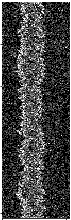
Figure 1: A noisy SEM image consisting of one line with two edges of dimension $64\times 1024$. The aspect ratio of the image has been altered to facilitate viewing. Reprinted with permission from Ref. 46.

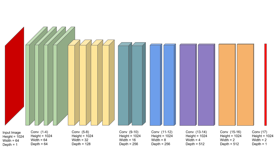
Figure 2: The 17 convolutional layers of EDGENet. Reprinted with permission from Ref. 30.

Because of the popularity of simulation within semiconductor metrology, our dataset consists of the simulated SEM images used earlier for References 29, 30 and 42. The generation of the dataset involves multiple steps. First, apply the Thorsos method[47, 48] with normally distributed random variables to simulate rough line edges or linescans which each follow a Palasantzas spectral model[49] characterized by three parameters: $\sigma$ is the line edge roughness (LER), i.e., the standard deviation of edge positions, $\alpha$ is the roughness (or Hurst) exponent and $\xi$ is the correlation length:

$$PSD(f)=\frac{\sqrt{\pi}\Gamma(\alpha+0.5)}{\Gamma(\alpha)}.\frac{2\sigma^{2}\xi}{(1+(2\pi f\xi)^{2})^{\alpha+0.5}}.$$

Each simulated edge has length 2.048 microns or, equivalently, 1024 pixels. Our edges have eight possible LER values ($\sigma$ = 0.4, 0.6, 0.8, 1.0, 1.2, 1.4, 1.6, 1.8 nm), nine possible Hurst/roughness exponent values ($\alpha$ = 0.1, 0.2, 0.3, 0.4, 0.5, 0.6, 0.7, 0.8, 0.9) and 35 possible correlation length values ($\xi$ = 6, 7, …, 40 nm) for a total of 2520 possible combinations of parameters ($\sigma$, $\alpha$, $\xi$). For each combination we produced eight edges.

The next step in generating the dataset is to apply a SEM simulator to generate the rough-line images from the simulated rough edges. A Monte Carlo-based simulator like JMONSEL[50] offers the most realistic simulated images, but we opt in References 29, 30 and 42 for the much faster simulator ARTIMAGEN[51, 52] to generate a large dataset and describe there the parameter settings we use; both simulators are publicly available. The images from ARTIMAGEN “closely mimic the noise, contrast and resolution, drift, vibration” of real SEM images[53]. Our 10080 images have dimension $64\times 1024$ pixels with pixel width $0.5$ nm and pixel height $2$ nm and incorporate a rough line at varying locations within the image of width 10 nm or 15 nm with two of the previously generated edges together with random backgrounds, a fixed edge effect, fine structure and Gaussian blur. The ARTIMAGEN library does not offer fractional edge positions, so the edge positions are rounded; this is a limitation of ARTIMAGEN. Rounding operations are not differentiable, so we do not use them in the implementation in the new final layer of EDGENet nor in the actual LER computations.

We have so far described our “original” image set. We apply a feature of the ARTIMAGEN library to produce ten images corrupted by varying levels of Poisson noise for each original image with electron density per pixel in the range $\{2,\ 3,\ 4,\ 5,\ 10,\ 20,\ 30,\ 50,\ 100,\ 200\}$. These 100800 images are our noisy image dataset. Our supervised learning dataset for the training of the original EDGENet consists of pairs of matrices $(x^{i},\ y^{i})$, where $x^{i}$ is a noisy image and $y^{i}$ is a $2\times 1024$ matrix of edge positions associated with corresponding original image. For the augmented EDGENet $y^{i}$ is now either the LER of the left edge of the original image or the LER of the right edge of the original image.

5 Auxiliary Neural Networks

Our first attempts[23] at using conformal prediction and quantile regression were preliminary and did not take advantage of our group’s earlier work on denoising. However, we now seek to use the relationship between the amount of noise in an image and the inaccuracies in an edge detection procedure for that image. The noise image presumably contains information to help a neural network predict a function of the residual, namely, $-\ln|y^{i}-g(x^{i})|.$ Our results support this intuition.

We propose three similar deep neural networks NCPMaxPoolNet, NCPLSTMNet, and NCPBLSTMNet that each improve upon the average interval lengths that we reported in Ref. 23. All of them begin with a CNN that learns multiple filter maps from the noise image and subsequently employ an individual feature extraction layer followed by a fully connected network that predicts the desired function of the residual. Each CNN contains a convolution layer of 64 filters followed by another with 128 filters followed by a third convolutional layer with 256 filters. All layers employ a 3$\times$3 kernel, 2$\times$2 stride length and equal padding. We initialize the convolution weights via Xavier uniform initialization and use the Rectified Linear Unit (ReLU) activation function. Each convolutional layer is followed by a batch normalization layer and a dropout layer with a 2% dropout rate. The output of this portion of each network is 256 feature maps of dimensions 64$\times$128.

The next set of layers reduce the dimensionality of the output filter maps and extract features to facilitate estimation. NCPMaxPoolNet uses a global max-pooling layer to reduce the $64\times 128\times 256$ dimensional output from the CNN to a $1\times 1\times 256$ vector. The NCPLSTMNet and NCPBLSTMNet networks follow the initial CNN layers with another convolution layer with 64 filters to produce 64 feature maps of dimension 32$\times$64 and subsequently apply a 4$\times$4 max-pooling layer to output feature maps of dimension 8$\times$16. The NCPLSTMNet output is reshaped into 64 vectors of length 128 and input to a Long Short Term Memory (LSTM) [54] layer with 64 cell units to produce a 64-dimensional vector. Since Bidirectional Long Short Term Memory (BLSTM) networks often outperform LSTM networks[55] the NCPBLSTMNet variant replaces the LSTM layer with a BLSTM layer.

All three network models end with a set of fully connected layers. NCPMaxPoolNet is designed to predict error estimates for both the left and right edges and consists of two branches of four fully connected layers with sixty-four, sixteen, four, and one neuron, respectively, each using the ReLU activation function. As reported in our earlier work [23], the ARTIMAGEN simulation process yields systematic differences in the left and right edge data mainly because of the application of Gaussian blur at $30^{\circ}$ to the horizontal x-axis, which results in random drift effects typically known as astigmatic effects. Therefore, one can construct more efficient prediction intervals by training separate models for each edge. For NCPLSTMNet and NCPBLSTMNet we use this strategy and use four fully connected layers with thirty-two, eight, four, and one neuron, respectively; the first three layers apply a Leaky ReLU [56] activation function and the fourth one applies a ReLU activation function. We use the mean absolute error loss function to train all three networks. As we will see, these strategies offer performance improvements over the basic version of conformal prediction.

Just as effective modeling is needed to create efficient normalized conformal prediction intervals, it is not immediately apparent how to effectively use quantile regression on high-dimensional image data. Our approach takes advantage of the strengths of our new normalized conformal prediction models together with the success of residual learning [57] and a variation of stacked generalization [58]. We propose three quantile regression neural networks QRMaxpoolNet, QRMaxpool-LSTMNet, and QRMaxpool-BLSTMNet and train separate models for the left and right edges. Each network inputs the EDGENet’s LER prediction along with estimates $\phi(x_{N}^{i})$ of the error measure $-\ln|y^{i}-g(x^{i})|$ associated with the desired miscoverage rate from the normalized conformal prediction model. QRMaxpoolNet inputs the EDGENet prediction and the estimated error measure from NCPMaxPoolNet. QRMaxpool-LSTMNet and QRMaxpool-BLSTMNet each take three inputs: the EDGENet prediction, the estimated error measure from NCPMaxPoolNet and either the estimated error measure from NCPLSTMNet or from NCPBLSTMNet. As depicted in Fig. 3, each network has one hidden layer and an output layer. The hidden layer is fully connected with a number of neurons equal to twice the number of network inputs. The output layer estimates the upper and lower quantile levels. The network architecture incorporates a residual connection between the EDGENet LER input and the output layer so that the model alters the LER prediction to output the endpoints of a prediction interval. These neural networks are trained using the pinball loss function [22], but the asymmetric Huber may offer more flexibility in meeting business goals [59]. Applying CQR to each of these networks yields models we call CQRMaxpoolNet, CQRMaxpool-LSTMNet, and CQRMaxpool-BLSTMNet.

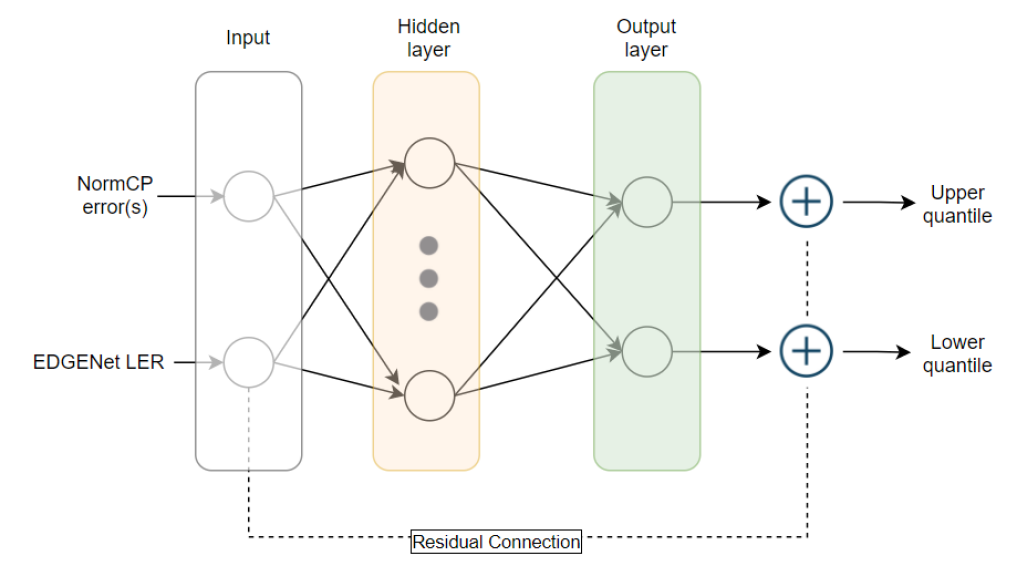
Figure 3: Quantile regression neural network architecture.

6 Experiments and Results

We now examine the results of the proposed schemes and present the coverage and interval sizes for both the left and right edges at a 10% miscoverage rate. As we mentioned earlier, there are systematic differences between the left and right edge data, so we gain more insight about the efficacy of the proposed techniques.

The six proposed neural network models were trained on an Intel Xeon E5-2680 v4 processor running at 2.4 GHz and a Tesla K80 GPU. We use hyperparameter optimization to choose values for the batch size, optimizers, and the learning rate and determine that a batch size of eighteen combined with an Adam[60] optimizer with a learning rate of 0.001 offers the best training performance over all models.

The 100800 noisy images are first normalized so that all values are in the range (0,1). We apply SEMNet to each noisy image to obtain its corresponding noise image. The noise image dataset is separated into a proper training set, a calibration set, and a test set. The combination of calibration and test sets consist of the 11520 noise images associated with correlation length $\xi$ in the set $\{10,\ 20,\ 30,\ 40\}$ nm which are partitioned into two sets of 5760 images for the calibration and test sets based on the corresponding original images to approximate exchangeability[23]; for each original image all ten corresponding noise images all belong to the same set. For the quantile regression neural networks, we calculate EDGENet’s LER predictions and the associated normalized conformal prediction error measures for each scheme for the entire dataset as part of the quantile regression procedure.

We present the coverage and interval statistics for the left and right edges at 10% miscoverage rate in Tables 1 and 2, respectively. Nearly all of the proposed conformal models outperform the conformal prediction and normalized conformal prediction schemes of Ref. 23, and in some cases the performance improvement is significant. The proposed normalized conformal prediction schemes perform particularly well on the left edge data. Quantile regression networks have been investigated for multiple applications and are known to have a tendency to undercover [61]; our quantile regression networks grossly undercover, but conformalization helps to address this problem even though the relative size of our calibration set is much lower than the recommendation of Ref. 41. In Ref. 23, we reported that EDGENet has more difficulty with prediction for right edge data compared with left edge data. Despite this, the proposed conformalized quantile regression models reduce the disparity between average interval lengths for the left edge and right edge data.

Table 1: Coverage and interval width summary statistics for left edge LER at 10% miscoverage rate

Method	Coverage	Average interval
	(%)	length (nm)
Conformal Prediction (CP)[23]	90.22	0.135
Normalized CP[23]	90.15	0.153
NCPMaxPoolNet	89.36	0.127
NCPLSTMNet	90.30	0.130
NCPBLSTMNet	90.43	0.124
QRMaxpoolNet	81.39	0.146
CQRMaxpoolNet	87.97	0.169
QRMaxpool-LSTMNet	71.39	0.094
CQRMaxpool-LSTMNet	88.18	0.134
QRMaxpool-BLSTMNet	79.60	0.096
CQRMaxpool-BLSTMNet	88.14	0.117

Table 2: Coverage and interval width summary statistics for right edge LER at 10% miscoverage rate

Method	Coverage	Average interval
	(%)	length (nm)
Conformal Prediction (CP) [23]	89.22	0.186
Normalized CP [23]	88.96	0.241
NCPMaxPoolNet	89.58	0.242
NCPLSTMNet	89.22	0.186
NCPBLSTMNet	89.24	0.181
QRMaxpoolNet	84.83	0.156
CQRMaxpoolNet	88.58	0.168
QRMaxpool-LSTMNet	65.59	0.077
CQRMaxpool-LSTMNet	89.01	0.128
QRMaxpool-BLSTMNet	75.64	0.096
CQRMaxpool-BLSTMNet	89.35	0.133

7 Ongoing Work and Conclusions

We are aware of the numerous and rapid advances related to attention mechanisms, and we are working to leverage attention in our distribution-free prediction interval models.

The semiconductor manufacturing community will continue to impact computing. Those who may benefit from continued advances in computing must help them develop more confidence in the role of deep learning and other forms of artificial intelligence for decision making. Distribution-free prediction intervals with coverage guarantees are an initial step to address this need, and much more research is required.