Systematic Comparison of Path Planning Algorithms using PathBench

Abstract

Path planning is an essential component of mobile robotics. Classical path planning algorithms, such as wavefront and rapidly-exploring random tree (RRT) are used heavily in autonomous robots. With the recent advances in machine learning, development of learning-based path planning algorithms has been experiencing a rapid growth. An unified path planning interface that facilitates the development and benchmarking of existing and new algorithms is needed. This paper presents PathBench, a platform for developing, visualizing, training, testing, and benchmarking of existing and future, classical and learning-based path planning algorithms in 2D and 3D grid world environments. Many existing path planning algorithms are supported; e.g. A*, Dijkstra, waypoint planning networks, value iteration networks, gated path planning networks; and integrating new algorithms is easy and clearly specified. The benchmarking ability of PathBench is explored in this paper by comparing algorithms across five different hardware systems and three different map types, including built-in PathBench maps, video game maps, and maps from real world databases. Metrics, such as path length, success rate, and computational time, were used to evaluate algorithms. Algorithmic analysis was also performed on a real world robot to demonstrate PathBench’s support for Robot Operating System (ROS). PathBench is open source.

1 Introduction

In robotics, path planning remains as an open problem, as a multi-objective optimization problem, to generate a feasible and continuous path that connects a system from its start to goal configuration. Various algorithms exist, yet the research on developing newer ones is still ongoing [1, 2, 3]. In particular, recently there is rapid growths in methods that rely on machine learning and deep neural networks, allowing to solve complex planning problems. This indicates the urgent need the community have to develop a unified benchmarking framework to compare the existing and new algorithms against metrics such as length and smoothness of paths, run time and memory consumption, and the success rate of the algorithms. In this work, we aim to solve this problem by presenting a modular simulation & benchmarking platform and conducting a comparative study, demonstrating how various algorithms on different hardware compare considering the metrics of interest. (See Fig. 1 and Fig. 2)

We compare various classical and machine-learning based path planning algorithms across a range of hardware, typically used in robotic applications, that produced Fig. 1. Extensive results are presented in Section 7. The results presented here are easily reproducible and extendable to other existing and future algorithms, using the unified platform, coined PathBench. These results are important in applications that seek Pareto optimality or require trades-offs between several performance metrics, such as execution time, path length, and trajectory smoothness. For instance, from Fig. 1, it is evident that A* is the fastest algorithm; however, it does not optimize for obstacle clearance. In contrast, VIN and MPNet, which are neural network-based planners, produce paths that are not nearly as close to obstacles.

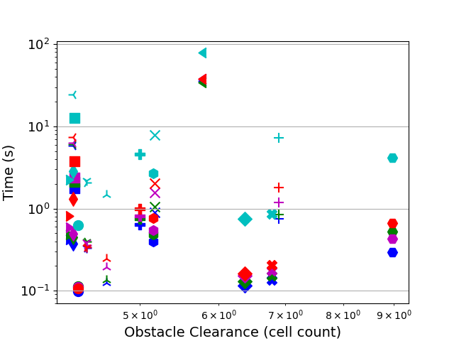
Figure 1: Scatter plot from comparative studies using various hardware systems that demonstrates obstacle clearance (higher is better) and time performance (lower is better) of algorithms. It is observed that obstacle clearance is consistent across different hardware systems and computation time of algorithms is faster in systems with more powerful CPU and GPU. To generate this figure, each algorithm, represented by a shape, was run on 3000 maps of size 64$\times$64, and the results were averaged. Additional analysis with plots generated by PathBench can be found in Sec. 7.2.

This comparative study presented utilizes PathBench, a motion planning platform that can be used to develop, assess, compare, and visualize the performance and behaviour of path planning algorithms. PathBench currently supports only grid map environments; however, it will be expanded to include continuous space and topological maps and algorithms in the future. The key contributions of this work include:

• Creation of an unified path planning development and benchmarking platform, that supports both 2D and 3D classical and learned algorithms. Existing machine learning based algorithms, such as value iteration networks (VIN) [4], gated path planning networks (GPPN) [5], motion planning networks (MPNet) [6], as well as Online LSTM [7], and CAE-LSTM [8] methods, are incorporated into PathBench. PathBench has a structured environment to facilitate easy development and integration of new classical and ML-based algorithms. The platform provides interfaces for algorithm visualization, rapid development, training, training data generation and benchmarking analysis. Waypoint Planning Networks (WPN) [9] is an algorithm developed within PathBench to showcase its feasibility.

• PathBench’s benchmarking features allow evaluation against the suites of added path planning algorithms, both classical algorithms and machine-learned models, with standardized metrics and environments.

• PathBench provides a ROS (Robot Operating System) real-time extension for interacting with a real-world robot. Examples have been provided on the GitHub of the project.

• Using PathBench, we provide a comparative analysis of a large suite of publicly available classical and learning-based path planning algorithms across different map types, datasets and hardware systems for point mass in 2D and 3D grid environments.

2 Related Work

In this section, classical and learned planning algorithms, and existing simulation & benchmarking frameworks are reviewed briefly.

2.1 Path Planning Algorithms

Based on map representation and algorithmic processing, there are various groups of path planning algorithms. For instance, graph search algorithms, such as Dijkstra [3], A* [11], and wavefront [12], commonly applied to grid and lattice maps, generate optimal results but are slow at applications with high-dimensional spaces such as robotic manipulators with many degrees of freedom. Sampling-based algorithms, such as rapidly-exploring random tree (RRT) [13] and probabilistic roadmap (PRM) [14], deal with the curse of dimensionality by sampling the configuration space or the state space to generate a path. However, these algorithms produce sub-optimal results. While graph search and sampling-based algorithms process the whole map, sensor-based planning algorithms, such as Bug1 and Bug2 [3, 15] plan only for a local view [16, 17]. This way the sensory data is taken into account. Numerical optimization algorithms, such as  [18], can also produce optimal results; however, they may become trapped in local minima. These algorithms optimize a cost function composed of kinematics constraints [19] or obstacle clearance and trajectory smoothness such as STOMP [20], CHOMP [21], and TrajOpt [22]. Some algorithms, such as [23], uses a combination of grid search and numerical optimization. Another important class of algorithms is the data-driven learning-based algorithms [24]. This algorithm can solve complex problems utilizing recent advances in high performance computing algorithms and hardware [8, 25, 26, 7, 27, 28, 29, 30, 6, 31, 32, 33, 34, 4, 5, 35, 36, 37].

2.2 Simulation and Benchmarking

Benchmarking of algorithms is the scientific approach of evaluation in the robotics community. In order to generate path planning benchmarks, reproducible experiments are required, which are easier in simulated environments. However, a common set of metrics, maps, and simulation environments has not been adopted for the evaluation of classical and learning-based path planning algorithms.

Currently, there is a variety of libraries relevant to the simulation and benchmarking of path planning algorithms, such as OpenRAVE [38], OMPL [39], MoveIt [40], SBPL [41], and OOPS_MP [41]. Most of these platforms have been designed for simulation and development of new planning methods. The ability to benchmark algorithms is also incorporated into OOPS_MP, MoveIt, and OMPL to facilitate algorithmic analysis [42, 41], but they do not support the evaluation and development of learning-based algorithms. Table 1 compares the key features of these frameworks with PathBench.

Table 1: Capabilities comparison for existing frameworks that focus on path planning algorithms. PathBench supports development, visualization, and benchmarking of classical and learned planning algorithms.

Platform	Visualization	Benchmarking	Sample-Based	Graph-Based	ML-Based
OpenRAVE	✓	$\times$	✓	$\times$	$\times$
OMPL	✓	✓	✓	$\times$	$\times$
MoveIt	✓	✓	✓	$\times$	$\times$
SBPL	✓	$\times$	$\times$	✓	$\times$
OOPSMP	✓	✓	✓	$\times$	$\times$
PathBench	✓	✓	✓	✓	✓

It is noticed that most existing benchmarking and simulation platforms do not support machine learning algorithms. However, newer projects such as iGibson [43], Habitat [44], and PyRobot [45] have started focusing on providing environments for artificial intelligence research in robotics.

PathBench also improves on previously developed platforms, but focuses presently on path planning development and benchmarking in grid space environments. The main advantages of PathBench over existing standardized libraries are its native support of machine learning path planning algorithms, as well as its simple and lightweight design, allowing fast prototyping for a research environment. A clean API for the algorithms also allows PathBench to be portable to standardized libraries and integration into iGibson and Habitat is possible. In addition, PathBench’s support for animated simulations and its simple interface allow it to be a suitable educational tool. It provides a standardized set of maps and metrics, so that benchmarking of new and existing algorithms can be performed quickly. We also provide a ROS real-time extension which converts the internal map move actions into network messages (velocity control commands) using the ROS APIs.

Further to these standard libraries, other works have sought to address the issue of benchmarking for motion planning. Althoff et al. provide a collection of benchmarks for motion planning of cars on roads, allowing reproducible results on problems [46]. By using OMPL and MoveIt, a benchmark of sampling-based algorithms used for grasping tasks of three manipulators has been formulated [47]. Benchmark for Autonomous Robot Navigation (BARN) is composed of ground navigation scenarios with emphasis on online path planning approaches, such as Dynamic Window Approach (DWA) and Elastic Bands (E-Band)  [48, 49, 50]. PathBench currently focuses instead on support of offline path planning methods in grid environments. On the other hand, Sturtevan provides a standard test set of maps, and suggests standardized metrics for grid based planning for gaming environments [51]. These maps have been ported into PathBench and are discussed further in Sec. 5.

Although comparative studies between classical path planning algorithms have been done for UAV and mobile robot navigation [52, 53], studies that compare both classical and learning-based path planning algorithms across different hardware systems are rare. Evaluations of algorithms on multiple hardware systems is especially essential in the field of robotics, due to potential size, weight, and power consumption constraints of embedded hardware devices for mobile robotics applications. For other robotics research problem, such as visual odometry and SLAM, there exist such studies. For instance, Delmerico and Scaramuzza have performed a benchmark comparison of monocular visual-inertial odometry algorithms across embedded hardware systems that are commonly adopted for flying robots [54]. SLAMBench series of papers conduct similar studies for a wide range of algorithms across various hardware [55, 56, 57]. Performance of path planning algorithms across commonly utilized hardware systems in robotics applications should also be examined, so that system-specific algorithmic benchmarks can be developed. PathBench facilitates cross-system evaluations and allows users to improve and select the appropriate algorithm for a desired task. In this paper, we perform a comparative study using PathBench and its feature for classic and learned planning algorithms. Fig. 8 showcases scatter plots that demonstrate trade-offs between algorithms across five different hardware configurations.

3 PathBench Platform

An overview of the architecture of PathBench is shown in Fig. 2. PathBench is composed of four main components: Simulator, Generator, Trainer, and Analyzer where infrastructures are created to link the four main components with other parts of the framework to provide general service libraries and utilities. The simulator is responsible for environment interactions and algorithm visualization. It provides custom collision detection systems and a graphics framework for rendering the internal state of the algorithms. The generator is responsible for generating and labelling the training data used to train the ML models. The trainer is a class wrapper over the third party machine learning libraries. It provides a generic training pipeline based on the holdout method and standardized access to the training data. Finally, the analyzer manages the statistical measures used in the practical assessment of the algorithms. Custom metrics can be defined, as well as graphical displays for visual comparisons. PathBench has been written in Python, and uses PyTorch [58] for ML.

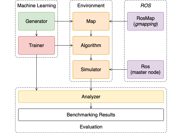
Figure 2: PathBench structure overview. Arrows represent information flow/usage ($A\xleftarrow{gets/uses}B$). The machine learning section is responsible for training dataset generation and model training. The Environment section controls the interaction between the agent and the map, and supplies graphical visualization. The ROS section provides support for real-time interaction with a real physical robot. The Evaluation section provides benchmarking methods for algorithm assessment.

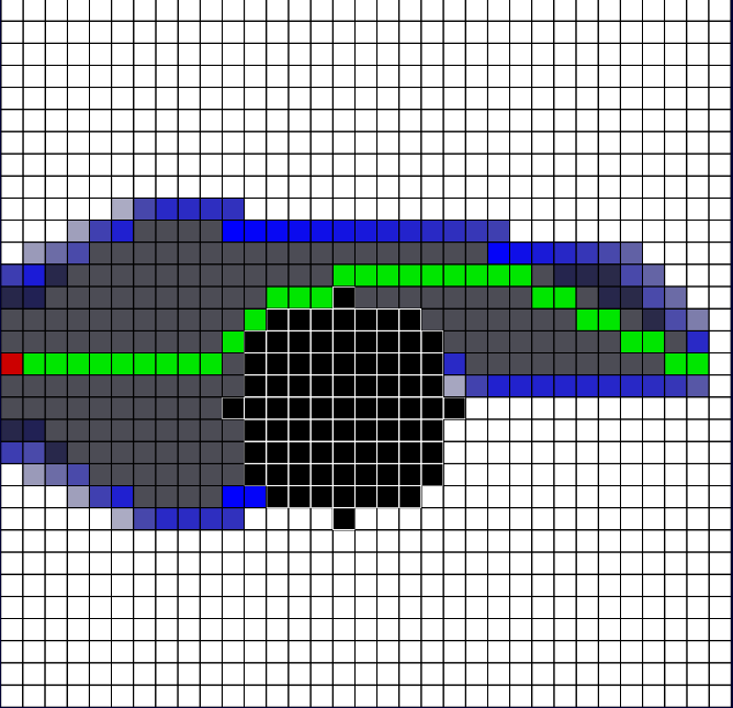
(a) A*

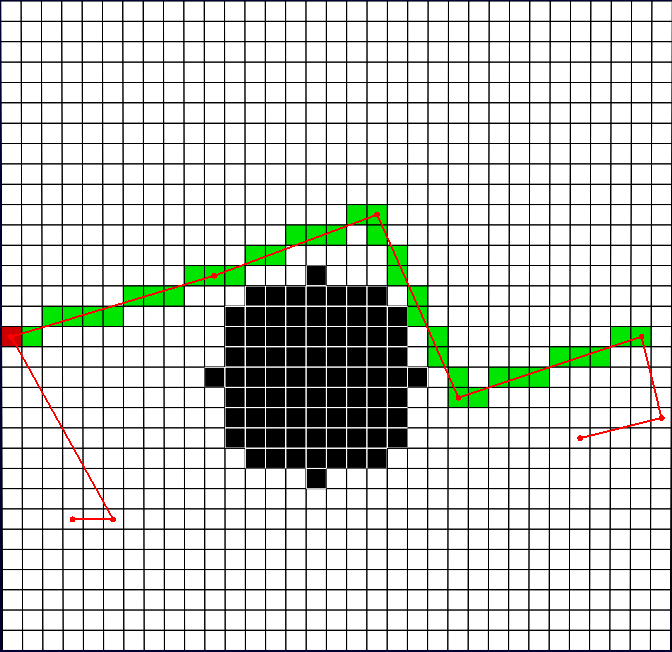
(b) Discrete RRT-Connect

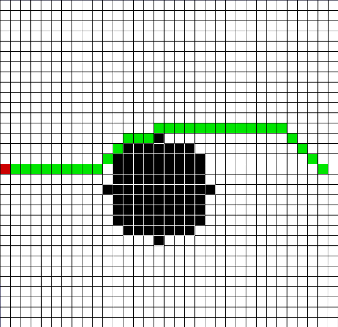
(c) GPPN

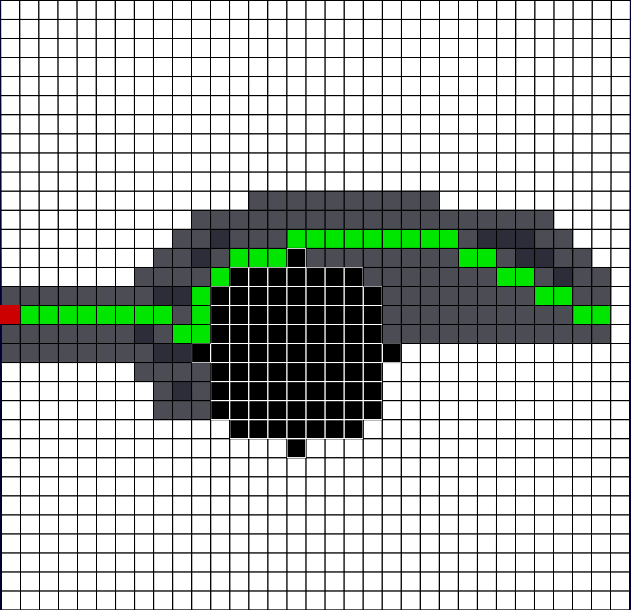
(d) WPN

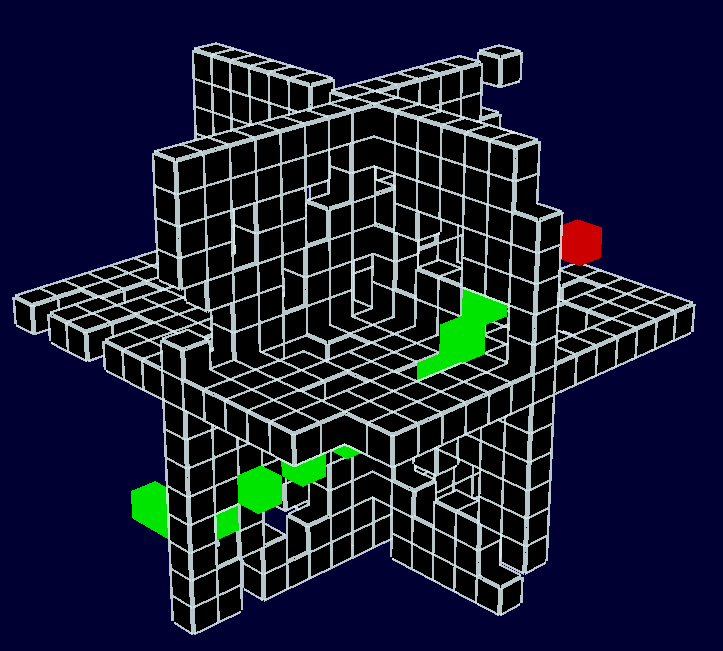
(e) A*

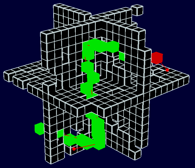
(f) Discrete RRT-Connect

Figure 3: The results of different classical and learned planners in PathBench. The red entity is the agent, light green cells show the path, with the green entity at the end of the path denoting the goal. The black entities are obstacles and everything else is custom display information (i.e. Dark gray represents the search space in (a) and (d), red represents edges of the sampling algorithm in (b), and blue shows the frontiers of the A* search space.) Discretized version of sampling-based algorithms [59] were used to ensure consistent performance in grid space.

3.1 Simulator

The simulator is both a visualizer and an engine for developing algorithms (Fig. 3). It supports animations and custom map display components which render the algorithm’s internal data. Simulator has a map that contains different entities such as the agent, goal and obstacles, and provides a clean interface that defines the movement and interaction between them. Therefore, a map can be extended to support various environments; however, each map has to implement its own physics engine or use a third party one (e.g. the pymunk physics engine or OpenAI Gym ). The current implementation supports three types of 2D/3D maps: DenseMap, SparseMap and RosMap, corresponding to static grid map, point cloud map, and grid map with live updates, respectively. Additionally, the simulator provides animations that are achieved through key frames and synchronization primitives. The graphical framework used for the visualization of planners and GUI is Panda3D [60]. Simulator configurations and visualization customizations can be directly controlled within the Panda3D GUI, see Fig. 4.

3.2 Generator

The generator executes the following four actions, each explained briefly below.

1) Generation. The generation procedure accepts as input, different hyper-parameters such as the type of generated maps, number of generated maps, number of dimensions, obstacle fill rate range, number of obstacle range, minimum room size range and maximum room size range. Currently, the generator can produce four types of maps: uniform random fill map, block map, house map and point cloud map, (See Fig. 5).

2) Labelling. The labelling procedure takes a map and converts it into training data by picking only the specified features and labels. Features that can be labeled include distance to goal, direction to goal, global obstacle map, local view, agent position, etc.

3) Augmentation. The augmentation procedure takes an existing training data file and augments it with the specified extra features and labels. It is used to remove the need for re-generating a whole training set.

4) Modification. A custom lambda function which takes as input a map and returns another map and can be defined to modify the underlining structure of the map (e.g. modify the agent position, the goal position, create doors, etc.).

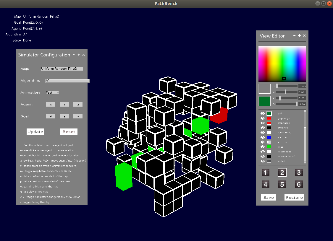
Figure 4: The GUI of the simulator is where configuration of the path planners, environments and customization of the visualization are made interactively. Simulator configuration window is used to set up path planning sessions, including the selection of algorithms, maps, and the start and goal points. View editor allows for adjustment of the simulation’s visualizations.

3.3 Trainer

The training pipeline is composed of six modules, explained below briefly.

1) Data Pre-processing. Data is loaded from the specified training sets, and only the features and labels used throughout the model are picked from the training set and converted to a PyTorch dataset.

2) Data Splitting. The pre-processed data is shuffled and split into three categories: training, validation and testing (Default data split is 60%, 20%, and 20%), according to the holdout method [61, 62]. The CombinedSubsets object is used to couple the feature dataset and label dataset of the same category into a single dataset. Then, all data is wrapped into its DataLoader object with the same batch size as the training configuration (Default size is 50). These parameters are configurable.

3) Training. The training process puts the model into training mode and takes the training DataLoader and validation DataLoader and feeds them through the model $n$ times, where $n$ is the number of specified epochs.

4) Evaluation. The evaluation process puts the model into evaluation mode and has a similar structure to the training process. The evaluation mode does not allow gradients to update.

5) Results Display. This procedure displays the final results from the three EvaluationResults objects (training, validation, testing) and final statistics such as the model loss are printed.

6) Pipeline End. At the end, the model is saved by serialising the model .state_dict(), model configuration, plots from results display process, and full printing log.

3.4 Analyzer

The analyzer is used to assess and compare the performance of the path planners. In addition to manually running a simulator instance to assess an algorithm, the analyzer supports the following analysis procedures:

• Simple Analysis. $n$ map samples are picked from each generated map type, and $m$ algorithms are assessed on them. The results are averaged and printed. Barplots and violinplots, for metrics discussed in Sec. 6, are generated with results from Simple Analysis.

• Complex Analysis. $n$ maps are selected (generated or hand-made), and $m$ algorithms are run on each map $x$ (Default is 50 runs for each map) times with random agent and goal positions. In the end, all $n\times x$ results are averaged and reported. Similarly to Simple Analysis, barplots and violinplots for selected metrics can be generated with results.

• Training Dataset Analysis. A training set analyzer procedure is provided to inspect the training datasets by using the basic metrics (e.g. Euclidean distance, success rate, map obstacle ratio, search space, total fringe, steps, etc. See the website of the project for all metrics and statistics).

4 Supported Path Planning Algorithms

The planning algorithms implemented into PathBench include the following algorithms and categories:

• Graph-based planners such as A*, Dijkstra, CGDS [63], and wavefront;

• Discrete sampling-based algorithms such as simple probabilistic roadmap (d-sPRM) and d-RRT with its variations such as d-RT, d-RRT*, and d-RRT-Connect; Moreover, additional sampling based algorithms from the Open Motion Planning Library (OMPL) are also added to improve benchmarking capability of PathBench;

• Sensory-based planning algorithms, e.g. Bug1 and Bug2 [16];

• Numerical optimization methods such as potential field algorithm [18];

• Learning-based path planning algorithms including Value Iteration Networks (VIN) [4], Motion Planning Networks (MPNet) [6], Gated Path Planning Networks (GPPN) [5], Online LSTM [7], CAE-LSTM [8], Bagging LSTM [9], and Waypoint Planning Networks (WPN) [9].

Additional classical or learning-based algorithms can be implemented to PathBench easily. The algorithms developed inside PathBench support step-by-step planning animation, which is an interesting feature for debugging and educational purposes.

We have included sampling-based planners, although they were originally designed for planning continuous space, and have competitive results in such settings. Graph-based or discrete sampling-based algorithms also exist, where instead of sampling from the free space, nodes of the graph are sampled for planning. Examples of such algorithms include [64, 59, 65], d-RRT [66], and d-RRT* [67]; however, as Branicky et. al state [64], “the performance of the RRT in discrete space is degraded by a decreased bias toward unexplored areas.” For benchmarking purposes, discretized versions of sampling algorithms (e.g. discretized RRT-Connect and discretized sPRM) were implemented within PathBench where each random sample is confined to an available grid cell.

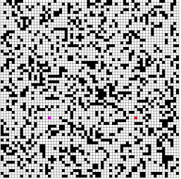
(a)

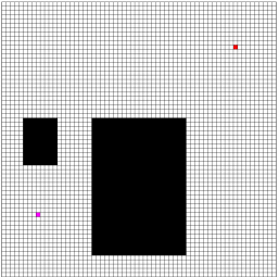
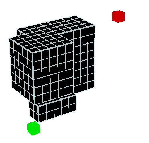
(b)

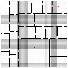
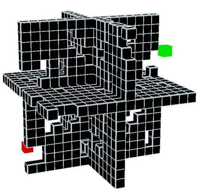
(c)

Figure 5: The 3 types of generatable grid maps are: (a) Uniform random fill ($64\times 64$ 2D and $16\times 16$ 3D dimensions, [0.1, 0.3] obstacle fill rate range), (b) Block map ($64\times 64$ 2D and $16\times 16$ 3D dimensions, [0.1, 0.3] obstacle fill rate range, [1, 6] number of obstacles range), (c) House atlas ($64\times 64$ 2D and $16\times 16$ 3D dimensions, [8, 15] minimum room size range, [35, 45] maximum room size range). (Note: Magenta colour is used as goal for all 2D maps as the green goal is difficult to spot.)

5 Supported Maps

The map is the environment of which simulation and benchmarking of algorithms are performed. Grid environments in 2D and 3D are presently used within PathBench. A Map contains different entities such as the agent, goal and obstacles, and provides a clean interface that defines the movement and interaction between them. Therefore, a map can be extended to support various environments. The following are supported 2D and 3D map types currently in PathBench.

5.1 Synthetic Maps

As mentioned previously in the Generator (Sec. 3.2), four synthetic map types can be created and used inside PathBench. The simplest map type, block maps, contains a random number of randomly sized blocks that act as obstacles. On the other hand, the map type of uniform random fill maps consists of single obstacles placed at random in the maps’ free spaces. The third map type, house maps, aims to mimic typical floorplans by placing obstacles in the form of randomly sized and partitioned walls. Lastly, 3D point cloud maps that contain a set of obstacles in an unbounded 3D space can also be generated and used in PathBench. The inclusion of point cloud maps is to facilitate the development and support of algorithms that work exclusively with point clouds, such as MPNet [6]. Different map types are included in PathBench, so that map-type specific performance of path planning algorithms can be analyzed further (See Fig. 5.)

5.2 Real Maps

Real-world maps can be utilized inside PathBench with the RosMap class. The RosMap extends 2D occupancy grid maps to integrate the gmapping [68] and other similar 2D SLAM algorithms by converting the SLAM output image into an internal map environment. The RosMap environment has support for live updates, meaning that algorithms can query an updated view by running a SLAM scan. The map uses simple callback functions to make SLAM update requests and convert movement actions into network messages using the ROS publisher-subscriber communication system.

5.3 External Maps

External maps can be imported into PathBench to diversify the datasets. Houseexpo [69] is a large dataset of 2D floor plans built on SUNCG dataset [70]. It contains 35,126 2D floor plans that have 252,550 rooms in total and can be used for PathBench benchmarking. In addition, other video game and real-world datasets can also be converted for PathBench use easily. 2D grid world and 3D voxel maps from video games, such as Warcraft III, Dragon Age and Warframe, and real world discretized 2D grid street maps from OpenStreetMaps geo-spatial database are implemented into PathBench to demonstrate the ease of integrating external datasets [51, 71], see Fig. 6. Benchmarking results on external maps are shown in Sec. 7.

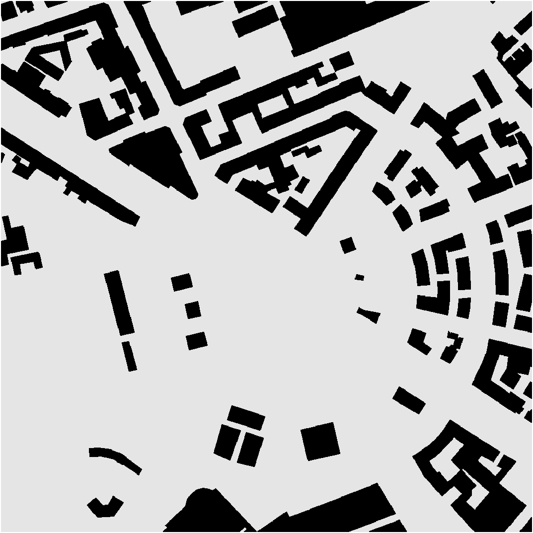
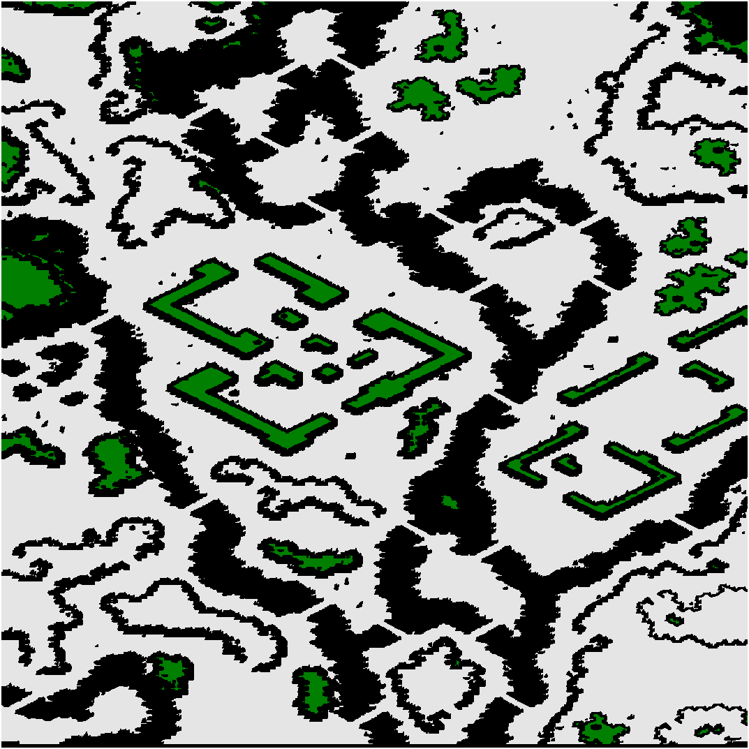
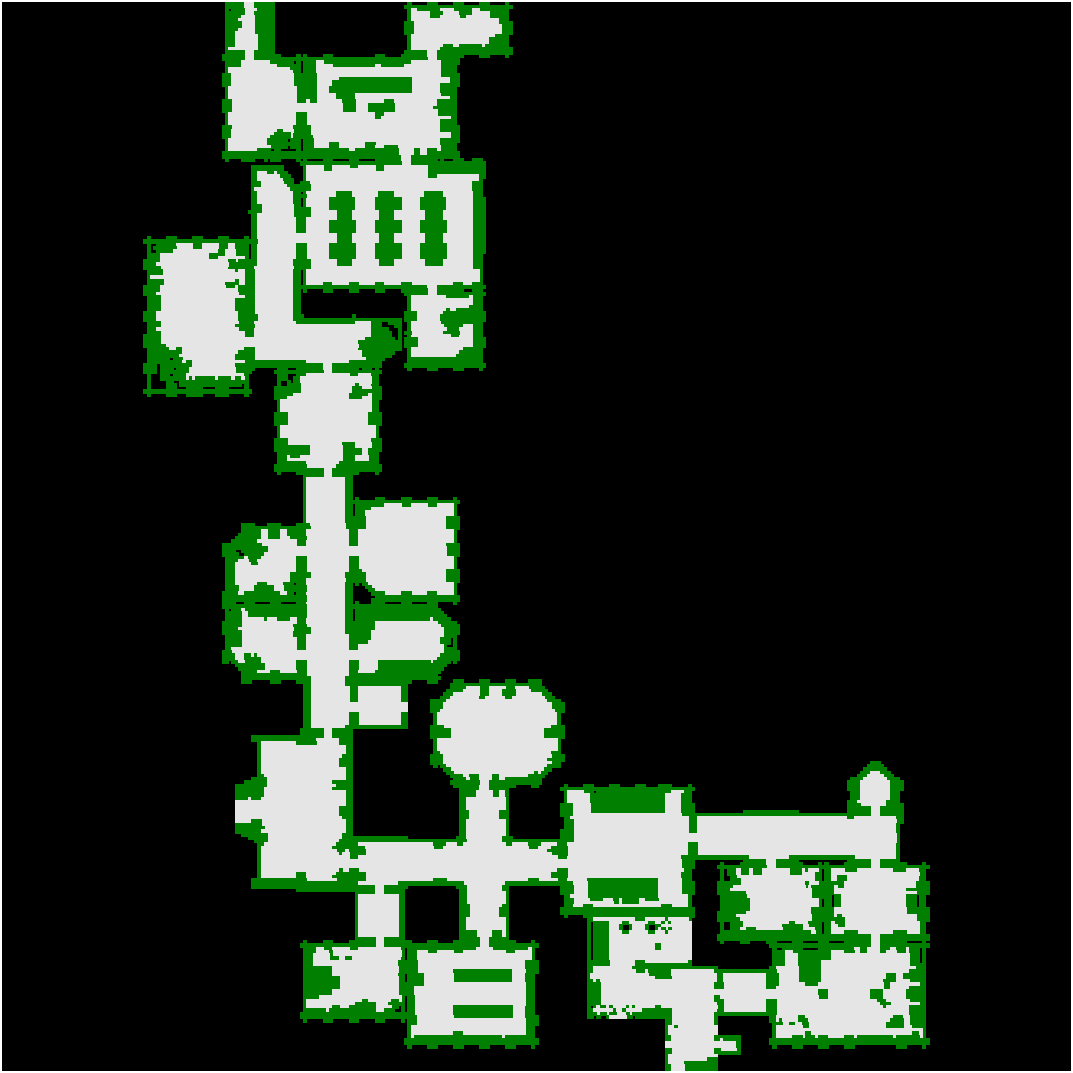
Figure 6: External maps can be ported into PathBench for benchmarking with ease. The maps above are from video games and real-world city [51].

6 Performance Metrics

In order to evaluate and benchmark performance of various algorithms inside PathBench, several metrics are chosen, including success rate, path length, distance left to goal when failed, time, path deviation, search space, memory consumption, obstacle clearance and smoothness of trajectory. Algorithm selection can be aided by evaluating the benchmarked results of task-specific metrics. The following outlines the metrics and rationales behind their selection.

1) Success Rate (%). The rate of success of finding a path, from start to goal, demonstrates the reliability of the algorithm.

2) Path Length (cell count). The total distance taken to reach the goal showcases the efficiency of the path generated.

3) Distance Left To Goal (cell count). The Euclidean distance left from the agent to the goal, in case of a algorithm failure. This shows the extent of the planning failure.

4) Time (seconds). The total time taken to reach the goal. Time required for planning is an important factor for real life robotics applications.

5) Path Deviation (%). The path length difference when compared to the shortest possible path, generated by A*.

6) Search Space (%). The amount of space that was explored and used to find the final path to the goal.

7) Maximum Memory Consumption (MB). The maximum amount of memory used during a path generation session. Memory usage could be a limiting factor for various robotics settings, thus being a relevant benchmarking metric.

8) Obstacle clearance (cell count). Obstacle clearance provides the mean distance of the agent from obstacles during traversal, where a higher value is typically more ideal.

9) Smoothness of trajectory (degrees). The average angle change between consecutive segments of paths shows how drastic and sudden the agent’s movement changes could be. A lower average angle change value provides a smoother trajectory. With discretized grid environments, smoothness of trajectory could produce misleading values due to large angle changes between each step. Smoothness of trajectory would be a more reliable metric in continuous map types where consecutive path segments can be defined with more clarity. PathBench has plans to explore continuous environments for learned manipulator planning approaches in the future.

Other than the metrics above, additional metrics can be implemented into PathBench if required. Nowak et al. provide potential metrics that could be added, including orientation error, number of collisions, number of narrow passages traversed and number of parameters to tune [72].

7 Experimental Results

In this section, several experiments, including algorithmic benchmarking and hardware system benchmarking, using PathBench, with classical and learned planners on different maps are presented. The algorithms are evaluated on 2D and 3D synthetic maps of varying sizes that are generated inside PathBench. In addition, video game and street maps from external datasets [51] are used for further algorithm benchmarking. Finally, algorithms are tested in ROS and Gazebo with PathBench’s ROS extension to highlight its ability to integrate with real world robotics applications.

7.1 Algorithmic Benchmarking

To begin, classical and learned algorithms, currently supported by PathBench, are benchmarked inside PathBench with different maps. All results are produced by PathBench on Ubuntu 18.04 with an Asus laptop with Intel Core i5-6200U CPU and Nvidia GeForce 940MX. This computer was chosen due to its GPU and processing power being widely available. For training of the learned algorithms, three types of synthetic map of size $64\times 64$ pixels were procedurally generated: uniform random fill map, block map, and house map. Fig. 5 shows samples of these maps. In these maps, start and goal points are chosen randomly. Evaluations are done on maps that have never been seen by the algorithms. To ensure that comparisons were done with the same trajectories between systems, the pseudorandom number generator’s random seed for sampling-based algorithms were initialized identically. We use the default values for the holdout method since there is a lot of training data available, but if one wants to change the amount of data for training and validation, it is also possible. The default batch size is 50, as it would fit on most GPUs.

Table 2: Results of classical algorithms: On 2D 64$\times$64 PathBench built in maps (3000 samples), 512$\times$512 city maps (300 samples), and video game maps with 800 to 1200 cells in dimension (300 samples). An Asus laptop with Intel i5-6200U CPU and Nvidia GeForce 940MX was used. The failed cases occur when there is no valid path towards the given goal.

map type	planner	path dev.(%)	distance left (if failed,cell count)	time (sec)	success rate (%)
PathBench	A* [11]	0.00	0.25	0.106	99.4
	Wavefront [12]	0.36	0.25	0.340	99.4
	Dijkstra [3]	0.00	0.25	0.338	99.4
	d-sPRM [14]	35.03	2.67	0.767	93.3
	d-RRT [13]	19.91	0.48	7.336	96.8
	d-RRT-Connect [73]	21.17	0.26	0.2458	99.33
City	A*	0.00	0.00	3.816	100.0
	Wavefront	1.08	0.00	8.468	100.0
	Dijkstra	0.00	0.00	9.928	100.0
	d-sPRM	123.64	13.68	5.377	93.6
	d-RRT	54.98	3.43	39.248	95.7
	d-RRT-Connect	65.08	5.35	3.489	96.6
Video Games	A*	0.00	0.00	31.567	100.0
	Wavefront	1.65	0.00	43.517	100.0
	Dijkstra	0.00	0.00	42.366	100.0
	d-sPRM	287.21	0.00	44.498	100.0
	d-RRT	128.90	64.38	64.881	42.6
	d-RRT-Connect	112.90	25.92	30.84	95.30

Table 3: Results of learned algorithms: On the same 2D 64$\times$64 PathBench built in maps (3000 samples), 512$\times$512 city maps (300 samples), and video game maps (300 samples) from Table 2. An Asus laptop was used to generate results. (Intel i5-6200U CPU and Nvidia GeForce 940MX)

map type	planner	path dev.(%)	distance left (if failed,cell count)	time (sec)	success rate(%)
PathBench	VIN [4]	5.25	29.55	1.796	18.2
	MPNet [6]	10.86	21.59	0.296	41.2
	GPPN [5]	6.83	27.56	2.018	30.3
	Online LSTM [7]	0.79	11.23	0.162	53.8
	CAE-LSTM [8]	0.99	12.57	0.207	48.7
	Bagging LSTM [9]	1.62	3.99	0.985	78.1
	WPN [9]	2.78	0.15	0.817	99.4
City	VIN	100.00	184.21	32.612	0.0
	GPPN	100.00	184.21	57.633	0.0
	Online LSTM	1.05	87.51	3.328	16.7
	CAE-LSTM	4.49	91.20	4.241	10.0
	Bagging LSTM	31.67	45.06	20.268	43.3
	WPN	8.44	0.00	13.816	100.0
Video Game	VIN	100.00	276.30	42.19	0.0
	GPPN	100.00	276.30	65.877	0.0
	Online LSTM	0.00	217.10	16.380	8.3
	CAE-LSTM	3.05	199.60	27.330	5.3
	Bagging LSTM	0.41	155.89	123.901	20.6
	WPN	10.55	0.00	110.307	100.0

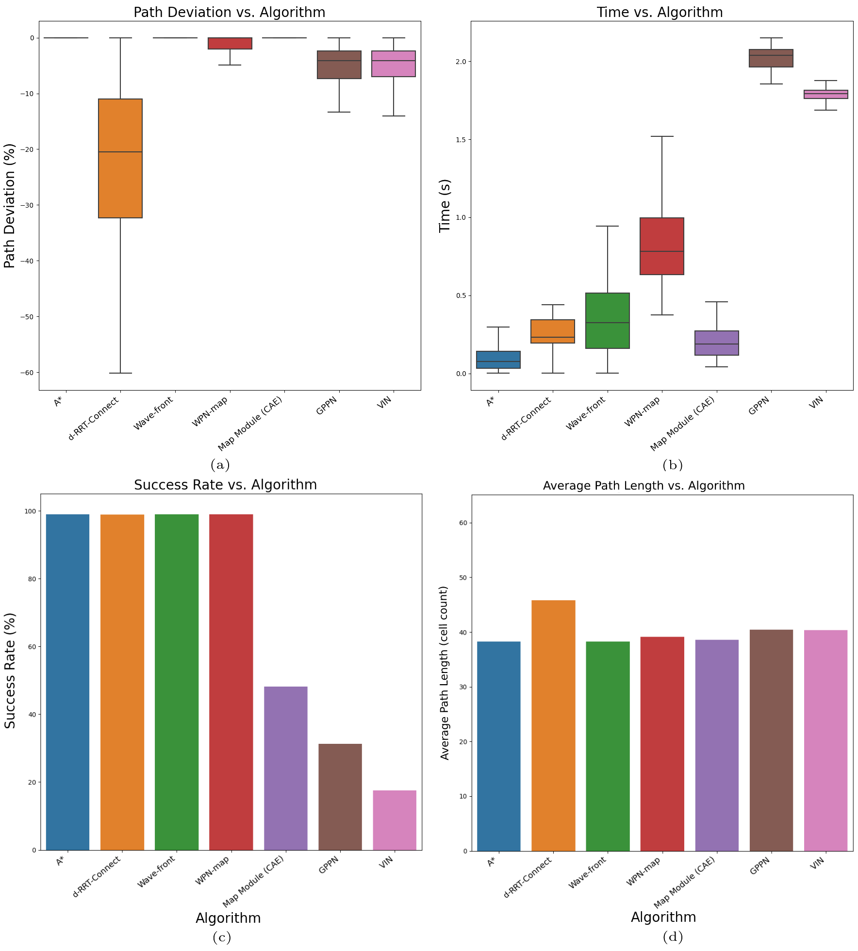
Figure 7: Graphical analysis of 2D benchmarking for classical and learned algorithms that is produced by PathBench’s analyzer. Results from Table 2 and Table 3 are used.

Table 4: Results of classical algorithms on 3D 28$\times$28$\times$28 PathBench built-in maps using an Asus laptop (3000 samples).

planner	success rate(%)	path len.(cell count)	path dev. (%)	time (sec)	path smooth- ness(deg.)
A*	100.0	20.69	0.00	0.475	0.28
Wavefront	100.0	21.27	0.51	6.118	0.11
Dijkstra	100.0	20.69	0.00	8.453	0.13
d-sPRM	100.0	36.87	16.18	0.248	0.37
d-RRT-Connect	99.7	38.22	17.56	0.097	0.41

7.1.1 2D Synthetic Maps: Simple Analysis

To demonstrate the benchmarking ability of PathBench and its support for the machine learning algorithms, all the algorithms described in Sec. 4 are analyzed against classical path planning algorithms in $64\times 64$ 2D PathBench maps. One thousand maps of each of the three types of PathBench maps were used. Table 2 and Table 3 present detailed comparative results for simple analysis of 3000 2D PathBench maps. Fig. 7 displays some of the key results in bar and violin plots.

7.1.2 2D External Maps: Complex Analysis

Both classical and learned algorithms were also benchmarked using the analyzer’s complex analysis tool, in order to demonstrate the framework’s ability to evaluate algorithm performance on specific map types. The analysis was performed on $n=30$ external city maps from OpenStreetMaps’ geo-spatial database [51], with 10 random samples collected for averaging of results on each $512\times 512$ map. Each map was run with $x=50$, selected as a reasonable value for hyperparameter. See Sec. 3.4 for parameter definitions. Thirty video game maps with height and width varying from 800 to 1200 cells were benchmarked in a similar manner. Results of benchmarking on video game and city maps are also listed in Table 2 and Table 3. The use of external environments in this experiment demonstrates the capability of PathBench to incorporate additional datasets.

7.1.3 3D Maps: Simple Analysis

To demonstrate PathBench’s support for 3D path planning, analysis of path planning algorithms on 3D $28\times 28\times 28$ PathBench maps was conducted. The benchmarking results that averaged algorithm performance on 1000 maps of each PathBench map type, uniform random fill map, block map, and house map, is shown in Table 4.

By looking at the 2D and 3D results, we can quickly assess some strengths and weaknesses of each planning approach. For example, the three graph-based algorithms all find a solution when one exists. A* and Dijkstra algorithms have path deviation of 0 percent, and wavefront also guarantees paths close to shortest possible lengths. d-RRT-Connect has much higher success rate than other sampling-based methods, while being considerably faster. The number and type of samples taken is a parameter that can be modified to configure sampling-based algorithms’ behaviour in PathBench. Although A* can generate the shortest path length in both 2D and 3D planning scenarios, d-RRT-Connect is capable of planning at a significantly faster time in 3D and larger 2D environments. Sampling path planning algorithms are also selected often for planning in higher dimensions and are the standard for manipulator motion planning. They will be focused on heavily as PathBench extends to higher dimensional planning. Machine learning algorithms, on the other hand, experience lower success rates for all map types. The success rates decrease greatly as maps become larger and more complex. For example, VIN and GPPN have shown to not scale well with the increase in map size and could not successfully provide any paths in the city and video game datasets. The drop in success rate of VIN and GPPN is consistent with what has been reported in the respective papers. Meanwhile, it is notable from the results of the benchmarking that GPPN outperforms VIN, suggesting that recurrent neural networks can help the algorithms to have a better performance. WPN is an exception with the ability to plan at 100% success rate for all map types when a solution is available and has a notably lower path deviation. This is due to WPN being a hybrid algorithm that incorporates A* in its way point planning approach. As learning-based algorithms, the three LSTM algorithms and MPNet have faster planning times and success rates than VIN and GPPN. However, machine learning algorithms’ path planning times in general are higher when compared to classical approaches, especially as the map size and complexity increases. MPNet was only tested on PathBench maps, due to constraint of the implementation used. The publicly available version of the network allowed encoding of a limited number of obstacles. It has a faster planning time than VIN, GPPN and WPN, but a higher path deviation. Performing this kind of simple and rapid analysis is trivial in PathBench.

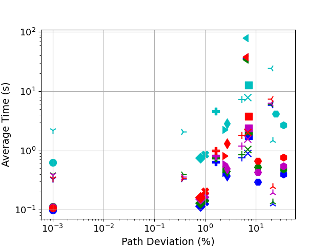
(a)

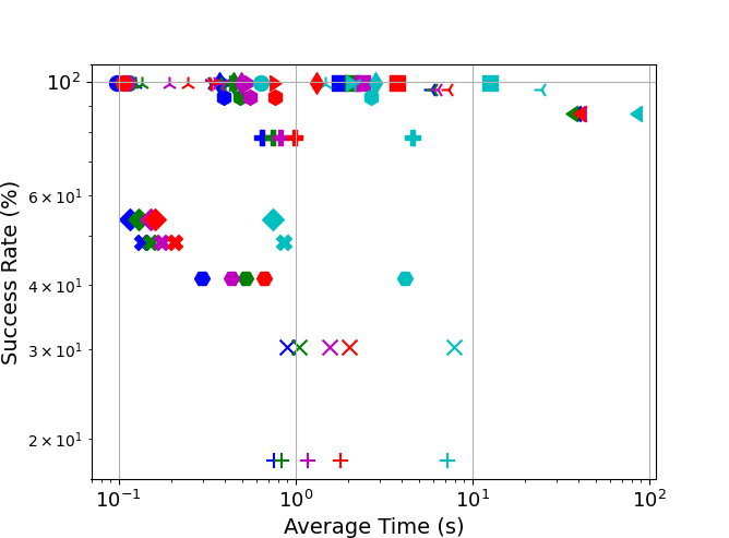
(b)

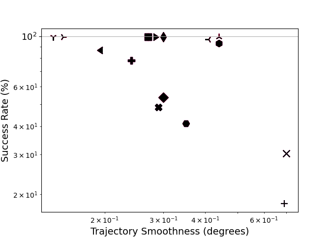
(c)

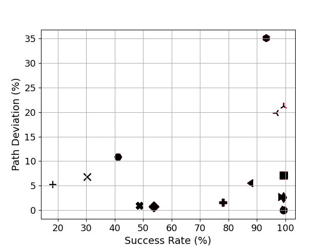
(d)

Figure 8: Scatter plots showing the performance of several classical and learned path planning algorithms. Each marker shape shows a different algorithm and different colors demonstrate the various hardwares. Performance metrics include the path deviation, success rate of the algorithm, trajectory smoothness, and the computation time. (Some markers overlap each other completely, due to values being the same across systems. These overlapped markers are indicated in black, as seen in plot (c) and (d).)

7.2 Hardware System Benchmarking

A comparative study using various hardware systems that are often used in the development and analysis of robotic applications has also been conducted. It demonstrates algorithm performance and consistency of PathBench’s benchmarking ability across different systems. Five hardware systems were used as follows:

1) Commodity Laptop. A commonly used laptop is chosen for becnhmarking due to its availability and use for rapid prototyping of path planning algorithms. It is equipped with Intel i5-6200U CPU and Nvidia GeForce 940MX GPU.

2) Gaming Laptop. The second laptop used possesses more computing power and has an Intel Core i9-10980HK CPU with Nvidia GeForce RTX 2080 GPU.

3) Intel NUC. The Intel NUC10i7FNK has an Intel i7-10710U CPU with no GPU and was also used to assess algorithms. It is a small form factor desktop computer and is popular in mobile robotic applications.

4) Compute Canada. Compute Canada’s Graham, a general purpose cluster for a variety of workloads, was utilized. For the Compute Canada analysis, Intel Xeon Gold 5120 CPU and Nvidia V100 GPU were used.

5) Raspberry Pi. Lastly, a Raspberry Pi Model 4b with ARM Cortex-A72 processor was also analyzed. It has no GPU and has 8GB of RAM. Raspberry Pi is commonly used in mobile robotics applications, making it an important device for path planning analysis.

The five hardware systems were analyzed on 64$\times$64 2D maps with one thousand maps for each of the three types of PathBench maps, i.e. uniform random fills, block maps, and house maps, shown in Fig. 5 (top row), totalling 3,000 maps.

7.2.1 Benchmarking Analysis

By examining Fig. 1 and Fig. 8, system specific algorithm performances are observed. Each scatter plot displays how optimal the algorithms are for two different metrics. Note that some markers overlap each other completely, as seen in plot Fig. 8-c and Fig. 8-d that have mostly black markers. These occur for the deterministic algorithms, such as A* and Dijkstra, in which the variation in hardware do not affect the performance metrics such as success rate or trajectory smoothness.

The computation times of the algorithms for hardware systems with more powerful CPUs are significantly faster as expected. Systems with more advanced GPUs have lower computation time for learning-based algorithms, such as VIN, GPPN and WPN, due to machine learning algorithms’ reliance on GPUs for matrice operations. A consistent spread across data points for different systems in the average time metric is observed. On the other hand, success rate (Fig. 8-b and c) and path deviation (Fig. 8-a and d) of both classical and learning-based algorithms share a strong consistency across the five hardware systems tested. Trajectory smoothness and obstacle clearance performance of classical and learned algorithms are also consistent across platforms.

Specific analysis between algorithms can be done as well. A* and WPN share the same trajectory smoothness in Fig. 8-c, as seen with the overlapped black markers. This is due to WPN’s use of A* for planning between waypoints. Dijkstra is expected to have similar trajectory with A*; however, the existence of multiple shortest possible paths on most maps led to a different trajectory smoothness value. On the other hand, GPPN was built upon VIN to improve its lower rate of planning success. In Fig. 8-b, GPPN can be observed to require more time for path computation in PathBench while having a much higher success rate than VIN. However, GPPN’s computation time can be improved significantly and surpass VIN’s performance on most systems, if CPUs with better processing power are used. This, combined with consistency of other metrics across systems, suggests that computation time of algorithms is the most important factor when selecting hardware systems for robotic applications.

Scatter plots seen in this section can be used to benchmark and select optimal algorithms and hardware for specific tasks and can be generated with PathBench’s analyzer. Such analysis, enabled by PathBench, allow system developers and algorithm designers to efficiently select the right algorithm for their application or benchmark and compare their new algorithm with existing ones. For instance, if for a particular application, a higher obstacle clearance is needed, according to Fig. 1, compared with A*, MPNet is a better choice assuming there is access to a good GPU such as NVidia GeForce RTX 2080, since MPNet is able to generate paths in $\approx$0.3 seconds with the best obstacle clearance values. If no GPU is available, still the algorithm works under a second, i.e. $\approx$0.5 seconds on NUC. This advantage, according to Fig. 8-b, comes at the cost of having less success rate ($\approx$41%) compared with other machine learning algorithms such as WPN ($\approx$99%) and Bagging LSTM ($\approx$78%).

7.3 Real-world Robot Interfacing

PathBench has the capability to natively interface with ROS and Gazebo to allow for seamless path planning for simulated and real world robotic applications. PathBench is able to visualize and plan for both fixed map environments and exploration environments. The planning is done in PathBench in real-time, and the control commands are sent to ROS to guide the robot. Fig. 9 visualizes different algorithms’ paths on real world maps acquired from SLAM performed in ROS. We can also demonstrate the live map capabilities of PathBench, using an algorithm with exploration capabilities. The robot can plan into known space, and also plan into the unknown environment, while the PathBench map is updated as it explores. This can also be seen in the supplementary video and GitHub, where the exploration is demonstrated.

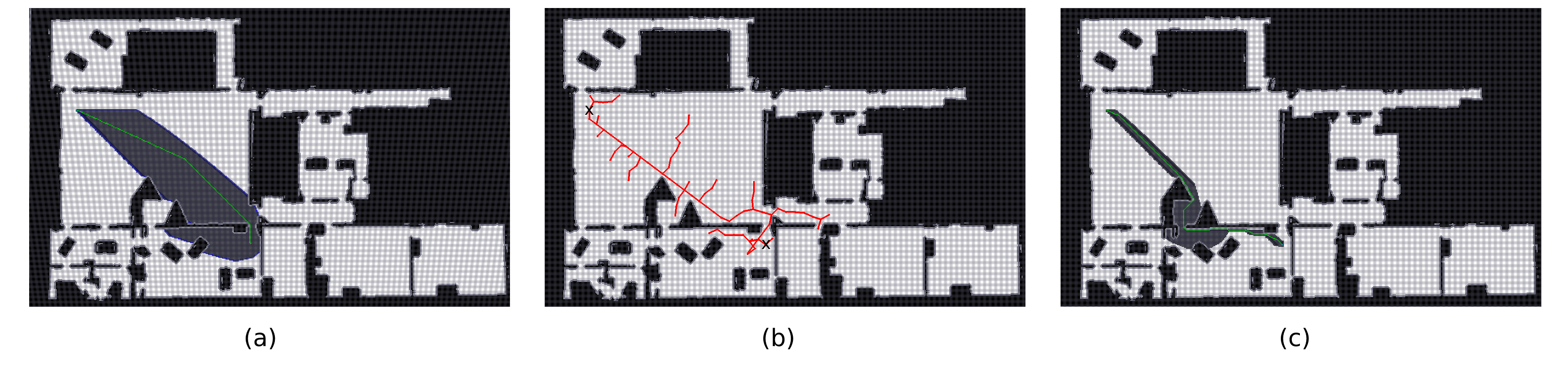
Figure 9: Visual comparison of planned paths on real world maps. a) A* b) d-RRT-Connect c) WPN (Note: Green represents the planned path. Grey is explored space and red is edges and nodes of sampling algorithms. Black Xs were used to denote the start and goal point for (b), since red edges cover the green path.)

8 Conclusion

PathBench presents a significant advantage in terms of developing and evaluating classical and learned motion planning algorithms, by providing development environment and benchmarking tools with standard and customizable metrics. PathBench has been demonstrated across a wide range of algorithms, datasets and systems with comparative studies using various hardware and planning environments in this paper. Further insights of algorithms, systems, and environments can be uncovered with extension to the PathBench framework.

In the future, PathBench will be extended to allow benchmarking and training of additional learning-based algorithms, along with support for higher dimensional planning with kinematic and dynamic constraints. We will also aim to integrate PathBench with notable simulated environments and planning datasets, such as iGibson and Habitat to offer more diverse and complex settings for benchmarking.

Funding

This work was partially funded by DRDC-IDEaS (CPCA- 0126) and EPSRC (EP/P010040/1).

Biographical Note

Hao-Ya Hsueh is a student at the Department of Mechanical and Industrial Engineering, Ryerson University. He is a member of Robotics and Computer Vision Lab at Ryerson University. His research interests include robotics, path planning, and computer vision.

Alexandru-Iosif Toma received M.Eng in Computing in 2019 from the Imperial College London. His research interests include machine learning, neural network, robotics, and computer vision.

Hussein Ali Jaafar is a student at the Department of Mechanical and Industrial Engineering, Ryerson University. He is a member of Robotics and Computer Vision Lab at Ryerson University. His research interests include mechatronics, computer vision, and robotics.

Edward Stow is a PhD Student in the Software Performance Optimisation Group at Imperial College London, having completed a M.Eng degree in Computing at Imperial College in 2020.

Riku Murai received M.Eng in Computing in 2019 from the Imperial College London. He is currently a PhD student in the Department of Computing at Imperial College London. His research interests include robotics and computer vision. In particular, the use of novel hardware and distributed computations.

Paul H J Kelly has been on the faculty at Imperial College London since 1989, has a BSc in Computer Science from UCL (1983) and has a PhD in Computer Science from the University of London (1987). He leads Imperial’s Software Performance Optimisation research group, working on domain-specific compiler technology.

Sajad Saeedi is an Assistant Professor at Ryerson University. He received his PhD in Electrical and Computer Engineering from the University of New Brunswick, Fredericton Canada. His research interests span over simultaneous localization and mapping (SLAM), focal-plane sensor-processor arrays (FPSP), and robotic systems.

References

- [1] González D, Pérez J, Milanés V, et al. A Review of Motion Planning Techniques for Automated Vehicles. IEEE Trans Intelligent Transportation Systems. 2016;17(4):1135–1145.
- [2] LaValle SM. Planning Algorithms. Cambridge university press; 2006.
- [3] Choset HM, Hutchinson S, Lynch KM, et al. Principles of Robot Motion: theory, algorithms, and implementation. MIT press; 2005.
- [4] Tamar A, Levine S, Abbeel P. Value iteration networks. CoRR. 2016;abs/1602.02867. Available from: http://arxiv.org/abs/1602.02867.
- [5] Lee L, Parisotto E, Chaplot DS, et al. Gated path planning networks. ICML. 2018;.
- [6] Qureshi AH, Miao Y, Simeonov A, et al. Motion planning networks: Bridging the gap between learning-based and classical motion planners. IEEE Transactions on Robotics. 2020;:1–9.
- [7] Nicola F, Fujimoto Y, Oboe R. A LSTM Neural Network applied to Mobile Robots Path Planning. In: IEEE International Conference on Industrial Informatics (INDIN); 2018. p. 349–354.
- [8] Inoue M, Yamashita T, Nishida T. Robot Path Planning by LSTM Network Under Changing Environment. In: Advances in computer communication and computational sciences. Springer; 2019. p. 317–329.
- [9] Alexandru-Iosif Toma, Hussein Ali Jaafar, Hao-Ya Hsueh, Stephen James, Daniel Lenton, Ronald Clark, Sajad Saeedi. Waypoint Planning Networks. In: 18th Conference on Robots and Vision (CRV), Burnaby BC Canada; 2021.
- [10] Toma AI, Hsueh HY, Jaafar HA, et al. PathBench: A Benchmarking Platform for Classical and Learned Path Planning Algorithms. In: 18th Conference on Robots and Vision (CRV), Burnaby BC Canada; 2021.
- [11] Duchoň F, Babinec A, Kajan M, et al. Path Planning with Modified A Star Algorithm for a Mobile Robot. Procedia Engineering. 2014;96:59–69.
- [12] Luo C, Krishnan M, Paulik M, et al. An Effective Trace-guided Wavefront Navigation and Map-building Approach for Autonomous Mobile Robots. In: Intelligent Robots and Computer Vision; Vol. 9025; 2014. p. 90250U.
- [13] LaValle SM. Rapidly-exploring Random Trees: A new tool for path planning ; 1998.
- [14] Kavraki LE, Svestka P, Latombe J, et al. Probabilistic roadmaps for path planning in high-dimensional configuration spaces. Vol. 12. ; 1996.
- [15] Rajko S, LaValle SM. A pursuit-evasion bug algorithm. In: ICRA; Vol. 2; 2001. p. 1954–1960.
- [16] Kamon I, Rivlin E. Sensory-based motion planning with global proofs. IEEE Transactions on Robotics and Automation. 1997;13(6):814–822.
- [17] Paull L, Saeedi S, Seto M, et al. Sensor-driven online coverage planning for autonomous underwater vehicles. IEEE/ASME Transactions on Mechatronics. 2013;18(6):1827–1838.
- [18] Hwang YK, Ahuja N. A potential field approach to path planning. IEEE Transactions on Robotics and Automation. 1992;8(1):23–32.
- [19] Ziegler J, Bender P, Schreiber M, et al. Making Bertha Drive—An Autonomous Journey on a Historic Route. IEEE Intelligent transportation systems magazine. 2014;6(2):8–20.
- [20] Kalakrishnan M, Chitta S, Theodorou E, et al. STOMP: Stochastic trajectory optimization for motion planning. In: IEEE International Conference on Robotics and Automation; 2011. p. 4569–4574.
- [21] Zucker M, Ratliff N, Dragan AD, et al. CHOMP: Covariant Hamiltonian optimization for motion planning. The International Journal of Robotics Research. 2013;32(9-10):1164–1193.
- [22] Schulman J, Duan Y, Ho J, et al. Motion planning with sequential convex optimization and convex collision checking. The International Journal of Robotics Research. 2014;33(9):1251–1270.
- [23] Dolgov D, Thrun S, Montemerlo M, et al. Path Planning for Autonomous Vehicles in Unknown Semi-structured Environments. The International Journal of Robotics Research. 2010;29(5):485–501.
- [24] Schwarting W, Alonso-Mora J, Rus D. Planning and decision-making for autonomous vehicles. Annual Review of Control, Robotics, and Autonomous Systems. 2018;1:187–210.
- [25] Chen N, Karl M, van der Smagt P. Dynamic Movement Primitives in Latent Space of Time-dependent Variational Autoencoders. In: IEEE-RAS International Conference on Humanoid Robots (Humanoids); 2016. p. 629–636.
- [26] Gupta S, Davidson J, Levine S, et al. Cognitive mapping and planning for visual navigation. In: CVPR; 2017. p. 2616–2625.
- [27] Qureshi AH, Yip MC. Deeply Informed Neural Sampling for Robot Motion Planning. In: IROS; 2018. p. 6582–6588.
- [28] Chamzas C, Shrivastava A, Kavraki LE. Using Local Experiences for Global Motion Planning. arXiv:190308693. 2019;.
- [29] Qureshi AH, Simeonov A, Bency MJ, et al. Motion planning networks. arXiv preprint arXiv:180605767. 2018;.
- [30] Qureshi AH, Dong J, Choe A, et al. Neural manipulation planning on constraint manifolds. IEEE Robotics and Automation Letters. 2020;5(4):6089–6096.
- [31] Bency MJ, Qureshi AH, Yip MC. Neural Path Planning: Fixed Time, Near-Optimal Path Generation via Oracle Imitation. arXiv preprint arXiv:190411102. 2019;.
- [32] Wu K, Abolfazli Esfahani M, Yuan S, et al. TDPP-Net: Achieving three-dimensional path planning via a deep neural network architecture. Neurocomputing. 2019;357:151 – 162.
- [33] Mohammadi M, Al-Fuqaha A, Oh JS. Path planning in support of smart mobility applications using generative adversarial networks ; 2018.
- [34] Choi D, jun Han S, Min K, et al. Pathgan: Local path planning with generative adversarial networks ; 2020.
- [35] Srinivas A, Jabri A, Abbeel P, et al. Universal planning networks. ICML. 2018;.
- [36] Levine S, Koltun V. Guided policy search. In: ICML; 2013. p. III–1–III–9.
- [37] Abbeel P, Coates A, Ng AY. Autonomous Helicopter Aerobatics Through Apprenticeship Learning. International Journal of Robotics Research. 2010;29(13):1608–1639.
- [38] Diankov R, Kuffner J. OpenRAVE: A Planning Architecture for Autonomous Robotics. Robotics Institute, Pittsburgh, PA, Tech Rep CMU-RI-TR-08-34. 2008;79.
- [39] Şucan IA, Moll M, Kavraki LE. The Open Motion Planning Library. IEEE Robotics & Automation Magazine. 2012;19(4):72–82.
- [40] Sucan IA, Chitta S. MoveIt ; 2014. https://moveit.ros.org; accessed .
- [41] Plaku E, Bekris KE, Kavraki LE. OOPS for Motion Planning: An Online, Open-source, Programming System. In: ICRA; Vol. 7; 2007. p. 3711–3716.
- [42] Moll M, Sucan IA, Kavraki LE. Benchmarking motion planning algorithms: An extensible infrastructure for analysis and visualization. IEEE Robotics Automation Magazine. 2015;22(3):96–102.
- [43] Shen B, Xia F, Li C, et al. iGibson, a simulation environment for interactive tasks in large realistic scenes. arXiv preprint. 2020;.
- [44] Savva M, Kadian A, Maksymets O, et al. Habitat: A Platform for Embodied AI Research. In: ICCV; 2019.
- [45] Murali A, Chen T, Alwala KV, et al. Pyrobot: An open-source robotics framework for research and benchmarking. CoRR. 2019;abs/1906.08236.
- [46] Althoff M, Koschi M, Manzinger S. CommonRoad: Composable Benchmarks for Motion Planning on Roads. In: IEEE Intelligent Vehicles Symposium (IV); 2017. p. 719–726.
- [47] Meijer J, Lei Q, Wisse M. Performance study of single-query motion planning for grasp execution using various manipulators. In: 2017 18th International Conference on Advanced Robotics (ICAR); 2017. p. 450–457.
- [48] Perille D, Truong A, Xiao X, et al. Benchmarking metric ground navigation. In: IEEE International Symposium on Safety, Security and Rescue Robotics (SSRR); IEEE; 2020.
- [49] Fox D, Burgard W, Thrun S. The dynamic window approach to collision avoidance. IEEE Robotics Automation Magazine. 1997;4(1):23–33.
- [50] Quinlan S, Khatib O. Elastic bands: connecting path planning and control. In: [1993] Proceedings IEEE International Conference on Robotics and Automation; 1993. p. 802–807 vol.2.
- [51] Sturtevant N. Benchmarks for grid-based pathfinding. Transactions on Computational Intelligence and AI in Games. 2012;4(2):144 – 148. Available from: http://web.cs.du.edu/~sturtevant/papers/benchmarks.pdf.
- [52] Radmanesh M, Kumar M, Guentert PH, et al. Overview of path-planning and obstacle avoidance algorithms for uavs: A comparative study. Unmanned Systems. 2018;06(02):95–118.
- [53] Wahab MNA, Nefti-Meziani S, Atyabi A. A comparative review on mobile robot path planning: Classical or meta-heuristic methods? Annual Reviews in Control. 2020;50:233–252.
- [54] Delmerico J, Scaramuzza D. A benchmark comparison of monocular visual-inertial odometry algorithms for flying robots. In: 2018 IEEE International Conference on Robotics and Automation (ICRA); 2018. p. 2502–2509.
- [55] Nardi L, Bodin B, Zia MZ, et al. Introducing SLAMBench, a performance and accuracy benchmarking methodology for SLAM. In: IEEE International Conference on Robotics and Automation (ICRA); 2015. p. 5783–5790.
- [56] Bodin B, Wagstaff H, Saecdi S, et al. SLAMBench2: Multi-Objective Head-to-Head Benchmarking for Visual SLAM. In: IEEE International Conference on Robotics and Automation (ICRA); 2018. p. 3637–3644.
- [57] Bujanca M, Gafton P, Saeedi S, et al. SLAMBench 3.0: Systematic Automated Reproducible Evaluation of SLAM Systems for Robot Vision Challenges and Scene Understanding. In: International Conference on Robotics and Automation (ICRA); 2019. p. 6351–6358.
- [58] Paszke A, Gross S, Chintala S, et al. Automatic Differentiation in PyTorch. In: NIPS Autodiff Workshop; 2017.
- [59] Morgan S, Branicky M. Sampling-based planning for discrete spaces. In: IEEE/RSJ International Conference on Intelligent Robots and Systems (IROS); Vol. 2; 2004. p. 1938–1945.
- [60] Goslin M, Mine MR. The Panda3D graphics engine. Computer. 2004;37(10):112–114.
- [61] Goodfellow I, Bengio Y, Courville A. Deep learning. MIT Press; 2016.
- [62] Nielsen M. Neural networks and deep learning. Determination Press; 2015.
- [63] Stow E, Murai R, Saeedi S, et al. Cain: Automatic code generation for simultaneous convolutional kernels on focal-plane sensor-processors. In: International Workshop on Languages and Compilers for Parallel Computing (LCPC); 2021.
- [64] Branicky M, Curtiss M, Levine J, et al. Rrts for nonlinear, discrete, and hybrid planning and control. In: IEEE International Conference on Decision and Control (ICDC); 2003. p. 657–663.
- [65] Hvezda J, Kulich M, Preucil L. Improved discrete rrt for coordinated multi-robot planning. In: International Conference on Informatics in Control, Automation and Robotics; 2018. p. 171–179.
- [66] Solovey K, Salzman O, Halperin D. Finding a needle in an exponential haystack: Discrete RRT for exploration of implicit roadmaps in multi-robot motion planning. The International Journal of Robotics Research. 2016;35(5):501–513.
- [67] Shome R, Solovey K, Dobson A, et al. dRRT*: Scalable and informed asymptotically-optimal multi-robot motion planning. Autonomous Robots. 2020;44(3-4):443–467.
- [68] Grisetti G, Stachniss C, Burgard W. Improved Techniques for Grid Mapping With Rao-Blackwellized Particle Filters. IEEE Transactions on Robotics. 2007;23(1):34–46.
- [69] Li T, Ho D, Li C, et al. Houseexpo: A large-scale 2d indoor layout dataset for learning-based algorithms on mobile robots ; 2019.
- [70] Song S, Yu F, Zeng A, et al. Semantic scene completion from a single depth image. CVPR. 2017;:1746–1754.
- [71] Brewer D, Sturtevant NR. Benchmarks for pathfinding in 3d voxel space. Symposium on Combinatorial Search (SoCS). 2018;.
- [72] Nowak W, Zakharov A, Blumenthal S, et al. Benchmarks for mobile manipulation and robust obstacle avoidance and navigation ; 2010.
- [73] Kuffner JJ, LaValle SM. RRT-connect: An efficient approach to single-query path planning. In: ICRA; Vol. 2; 2000. p. 995–1001.