Fast and Data Efficient Reinforcement Learning from Pixels via Non-Parametric Value Approximation

Abstract

We present Nonparametric Approximation of Inter-Trace returns (NAIT), a Reinforcement Learning algorithm for discrete action, pixel-based environments that is both highly sample and computation efficient. NAIT is a lazy-learning approach with an update that is equivalent to episodic Monte-Carlo on episode completion, but that allows the stable incorporation of rewards while an episode is ongoing. We make use of a fixed domain-agnostic representation, simple distance based exploration and a proximity graph-based lookup to facilitate extremely fast execution. We empirically evaluate NAIT on both the 26 and 57 game variants of ATARI100k where, despite its simplicity, it achieves competitive performance in the online setting with greater than 100x speedup in wall-time.

1 Introduction

Deep Reinforcement Learning (DRL) has become the standard approach to tackle complex non-linear sequential decision making problems exhibiting a high number of observational variables (Li 2017), a subset of which are image, or pixel, based. Although tabular Reinforcement Learning (RL) algorithms will learn (and in fact provably converge) in such environments, they are too slow to be practically useful. Policy and value function parametrization is thus typically used to facilitate learning, which has led to several breakthrough results  (OpenAI 2019; Badia and Piot 2020).

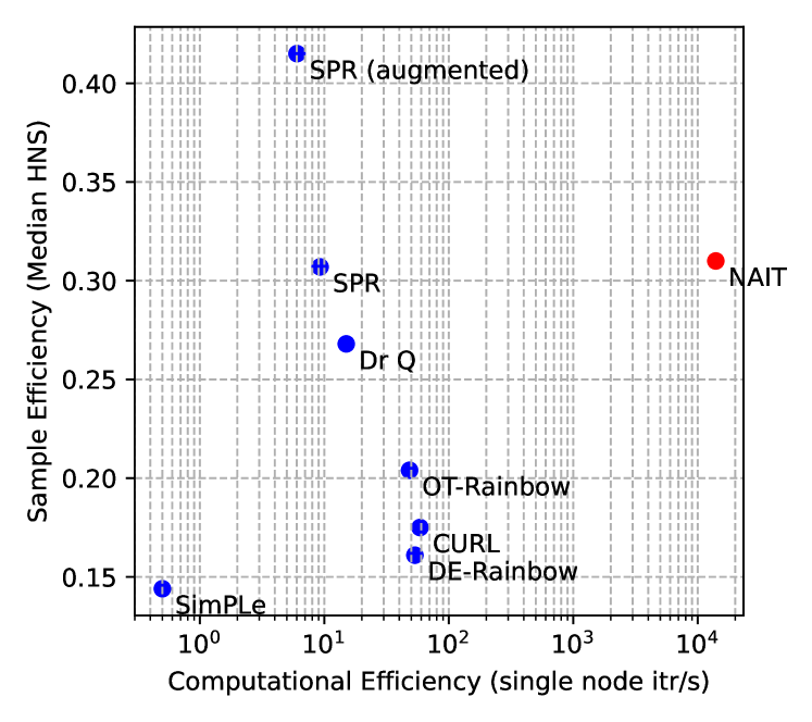
Figure 1: Comparison of our approach to other online sample efficient RL algorithms baselined on ATARI100k. NAIT achieves a $>$100x speedup over all other methods and is only outperformed in terms of median HNS by augmented SPR. Up and to the right is better. Algorithm labels are provided in Related Work.

Advances in raw performance, however, have been achieved at the cost of increased sample, and computational complexity. Agent 57 (Badia and Piot 2020) for example, requires 256 actors collecting approximately 57 years of real-time game play per game. For systems tackling more complex environments, these numbers are significantly higher. In an online, real-world setting this presents a major roadblock and, as a consequence, research attention has begun to shift towards improving sample efficiency with the goal of broadening the applicability of Deep Reinforcement Learning (DRL) in real world control and robotics. In these domains, sample efficiency is critical as the cost of each interaction is high; a physical robot must actually move. Improvements in sample efficiency, however, typically come at the cost of increased computational complexity, where additional CPU cycles are used to “squeeze” more from the available data, through a learned model  (Hafner et al. 2019), data augmentation  (Laskin et al. 2020), or similar.

The dominant evaluation framework for online RL algorithms remains simulated environments. In this setting, high computational complexity is not a bottleneck on performance. It does, however, decrease the practical relevance of the associated results by increasing the cost (in dollar terms), and thus reducing accessibility (Henderson et al. 2018). Scientific progress in the area is also impacted, as is visible in the fact that the high computational cost of SimPLe (Kaiser 2019) was one cause of the choice to evaluate on the 26 game “easy exploration” subset of the full 57 game suit, which made comparison to previous work difficult. It also make comparisons difficult, and expensive, for subsequent authors.

Computationally efficient approaches increase the scale at which algorithms can operate. For this reason several works have made attempts to speed up the evaluation simulators, such as CuLE for ATARI (Dalton, Frosio, and Garland 2019). Few, however, have focused on improving the computational efficiency of the RL algorithms themselves, instead focusing on distributed implementations (Stooke and Abbeel 2018), or the use of specialized hardware (Cho et al. 2019). Increasing the wall-clock speed with which decisions can be reached also directly increases the responsiveness of the system, which greatly simplifies tasks such as tracking and control (Wagner et al. 2010).

In this paper, we present Nonparametric Approximation of Inter-Trace returns (NAIT), an algorithm that is both computation and sample efficient. NAIT makes use of fast approximate k-nearest neighbour algorithms to generalise locally, and approximate a value function from stored memory. We combine this with a novel inter-trace update that provides the stability of episodic returns as well as the ability to immediately learn from an experience prior to completion of the episode (an advantage that is particularly pronounced in the low sample domain). We make use of a Discrete Cosine Transform (DCT) based transformation as the state representation, with no use of a learned encoder, prior knowledge, domain specific observation transformations or data augmentation.

We focus our evaluation on the ATARI100k suite of environments  (Kaiser 2019) in the online setting. Our approach is able to achieve 0.31 Median Human Normalized Score (MHNS), outperforming several previous state-of-the-art approaches such as Dr. Q (Kostrikov, Yarats, and Fergus 2020) and CURL (Srinivas, Laskin, and Abbeel 2020), despite making no use of a learned representations. In addition to this high level of sample efficiency, our approach is over two orders of magnitude faster than the current state of the art, SPR (Schwarzer et al. 2020), in terms of wall-time. In a single thread, NAIT is able to complete training for one environment in 7.2 minutes, where SPR requires 3.5 hours on the same GPU-enabled node. We examine our approach with ablation and sensitivity analysis, demonstrating the ability of NAIT to trade-off performance for speed, as well as a high level of robustness across hyperparameter values. Because of NAIT’s low execution time, we are able to provide baseline results under multiple evaluation settings and sample budgets, providing a strong baseline for future work.

2 Related Work

Recently significant focus has turned towards sample efficient RL in image-based environments. SimPLe (Kaiser 2019) consists of a novel network architecture used to model ATARI forward dynamics in the observation space, integrated within a Dyna-style (Sutton 1990) training loop. This work introduced the ATARI100k benchmark, and achieved $0.144$ median human normalised score (MHNS), significantly outperforming Rainbow (Hessel et al. 2018) and PPO (Schulman et al. 2017). Data Efficient Rainbow (DE-Rainbow) (van Hasselt, Hessel, and Aslanides 2019) was introduced to make use of more frequent value network updates per environment step, matching the update/step ratio used in SimPLe and achieved 0.161 MHNS while making no use of a learned model. Concurrently, Kielak presented OT-Rainbow (Kielak 2020), a similarly “over-trained” but otherwise unaltered version of rainbow capable of achieving $0.26$ MHNS.

Several works have identified representation learning as the bottleneck in this domain and have proposed techniques to accelerate it. CuRL (Srinivas, Laskin, and Abbeel 2020) introduced an auxiliary contrastive loss able to be utilized within existing RL algorithms. Dr. Q  (Kostrikov, Yarats, and Fergus 2020), focused solely on image augmentation (random shifts and random crops of observations), and demonstrated their inclusion raised the performance of an efficient DQN implementation from $0.058$ to $0.284$ MHNS. SPR (Schwarzer et al. 2020) proposes a latent space forward dynamics model, combined with an auxiliary prediction loss, that achieves 0.415 MHNS when combined with an augmentation scheme similar to that in Dr. Q.

Recently, several works such as APT (Liu and Abbeel 2021) and VISR (Hansen et al. 2019) have considered an additional unsupervised pretraining phase prior to online learning. In this setting, agents are provided a 250M frame budget with no environment rewards, after which rewards are restored for the standard 100k steps. Although we do not adopt this setting to evaluate out agent, we include several results to help contextualize the performance of NAIT.

Non-parametric, or lazy learning  (Sutton and Barto 1998) has been applied to ATARI previously. In the original work proposing the ALE environment (Bellemare et al. 2015), a Locality Sensitive Hashing (LSH) algorithm was proposed to convert pixel observations to binary features for SARSA($\lambda$). Linear learners ingesting fixed features were examined in (Liang et al. 2016), and remain strong baselines. In Model Free Episodic Control (MFEC) (Blundell et al. 2016), a gaussian random projection to a 64-dimensional latent space is used on ATARI frames, however performance is poor, possibly due to the small latent space dimensionality chosen. Berariu et. al. (Berariu and Gogianu 2017) augmented MFEC with sparse projections (Achlioptas 2003) along with variance normalisation in the projected space and demonstrated a improvement in performance, along with significant computational gains on ATARI.

3 Method

3.1 Background

We consider the standard formulation and notation (Sutton and Barto 1998) of an agent interacting with some environment at discrete time steps to maximise total expected reward. The environment is modelled as a Partially Observable Markov Decision Process (POMDP) $\left(\mathcal{O},\mathcal{A},P,r,\gamma\right)$ with a $D$ dimensional observation space $o\in\mathcal{O}:\mathbb{R}^{D}$ and discrete action space $a\in\mathcal{A}$. Traces are denoted as $\tau=\{(o_{0},a_{0},r_{0}),(o_{1},a_{1},r_{1}),\ldots\}$. $P=\text{Prob}(o_{t}^{\prime}|o_{\leq t},a_{\leq t})$ denotes the transition probability dynamics, $r:\mathcal{O}\times\mathcal{A}\rightarrow\mathbb{R}$ denotes the reward function and $\gamma\in[0,1)$ denotes a discount rate. We make use of a fixed projection $\phi:\mathbb{R}^{4\times D}\rightarrow\mathbb{R}^{F}$, to convert a stack of four observations (as is standard in ATARI) to a more compact space $s\in\mathcal{S}:\mathbb{R}^{F}$, $s_{t}=\phi\left(o_{t},o_{t-1},o_{t-2},o_{t-3}\right)$ where $F\ll D$. We treat $s$ as the base state henceforth, with $P=\text{Prob}(s_{t}^{\prime}|s_{t},a_{t})$ and $r_{t}=r(s_{t},a_{t})$. The discounted return from state $s_{t}$ and action $a_{t}\in\mathcal{A}$ taken at time $t$, is defined as $G(s_{t},a_{t})\doteq\sum_{k=t}^{H}\gamma^{k-t}r(s_{k},a_{k})$ where $H$ is the time horizon of the episode. For brevity, we often abbreviate this as $G_{t}=G(s_{t},a_{t})$ indicating the return from time $t$ onwards. If a range is specified as in $G_{t:T}$, this denotes the return from time $t$ until $T$. Our goal is to learn the optimal policy $\pi^{*}(s_{t})$ that maximises $\mathbb{E}_{P}\left[G(s_{t},a_{t})\right]$ for all $s_{t}\in\mathcal{S}$ where $a_{t}\sim\pi^{*}(s_{t})$. We make use of a memory $M$, where $M_{a}(s)$ refers to the value in memory for action $a$ and state $s$.

Algorithm 1 NAIT: Training and Acting

  Initialise: Memory $M_{a}\rightarrow\{\}$ for all $a\in\mathcal{A}$

  while training do

     $o\leftarrow$ reset environment, empty trace history $\tau\leftarrow\{\}$, $\mathbf{G}\leftarrow\{\}$, $\mathbf{\Gamma}\leftarrow\{\}$, $M^{\prime}_{a}\xleftarrow{\text{copy}}M_{a}$ for all $a$

     for $t=0$ to epsisode horizon $H$ do

        Get DCT representation $s\leftarrow\phi\left(o_{t},o_{t-1},o_{t-2},o_{t-3}\right)$

        for $a\in\mathcal{A}$ do

           Get estimate of $Q(s,a)$ using a kernel $K(s,s^{\prime})$, set of neighbours $L(s,a)=\{s_{1},\dots,s_{k}\}$

           $\qquad Q(s,a;k)=\begin{cases}M_{a}(s)&s\in M_{a}\\ \frac{\sum_{s^{\prime}\in L(s,a)}K\left(s,s^{\prime}\right)M_{a}(s^{\prime})}{\sum_{s^{\prime}\in L(s,a)}K\left(s,s^{\prime}\right)},&s\notin M_{a},\;|M_{a}|\geq k\\ 0&s\notin M_{a},\;|M_{a}|<k\end{cases}$

        end for

        $\pi(s)=\operatorname*{arg\,max}_{a\in\mathcal{A}}Q(s,a)$ breaking ties with $\pi_{\text{tiebreak}}(s)\sim\text{softmax}_{a\in\text{C}}\left(\frac{1}{k}\sum_{s^{\prime}\in L(s,a)}||s-s^{\prime}||_{2}^{2}\right)$

        Act $o,r\leftarrow\text{env}(\pi(s))$

        Add $(s,a)$ to $\tau$

        Get inter-trace targets (Alg. 3) and Update($\tau,\mathbf{Q}_{\textrm{IT}}$) (Alg. 2)

     end for

     Get final returns and Update($\tau,\mathbf{G}$) (Alg. 2)

  end while

At a high level, our approach acts by representing all observations via a fixed projection, calculating Q-values via local approximation, and updating these values iteratively as new rewards are encountered. The final algorithm is shown in Algorithm 1. We outline each component below.

3.2 Representation

As a fixed representation, we use a Discrete Cosine Transform (DCT) and select the first $F$ DCT coefficients ordered by frequency. The major advantage of the DCT as representation is that it is able to capture broad detail about the image extremely compactly, while being fast to compute, as $\mathcal{O}(D\log D)$ implementations based on the FFT exist. This is faster even than a random projection at $\mathcal{O}(FD)$ for many values of $F$. We make use of DCT II, an orthonormal transform $\mathbb{R}^{N}\rightarrow\mathbb{R}^{N}$,

$$\text{DCT:}\,X_{i}=\sum_{n=0}^{N-1}x_{n}\cos\left[\frac{\pi}{N}\left(n+\frac{1}{2}\right)i\right]i=0,\ldots,N-1.$$ (1)

We wish to apply this to the frame-stack obtained from the environment, and thus stack the four frames in a 2x2 grid to ensure equal weighting of vertical and horizontal frequencies, and apply the 2D DCT II. To compress the state, we discard high frequency coefficients and select the top $F$;

$$s_{t} =\phi\left(o_{t},o_{t-1},o_{t-2},o_{t-3}\right)$$ (2)

$$=\left[\text{DCT}\left(\text{DCT}\begin{bmatrix}o_{t}&o_{t-1}\\ o_{t-2}&o_{t-3}\\ \end{bmatrix}^{T}\right)^{T}_{ij}\right]_{0\leq i,j\leq\sqrt{F}}.$$

As the DCT is the only component of our approach specific to images, we also present results with domain-agnostic random projections as the representation (see Table 3). A random projection transforms the observation data (of dimension $D$) to a lower dimensional space (of dimension $F$) $\phi:x\rightarrow x\textbf{R}$, where $\textbf{R}\in\mathbb{R}^{D\times F}$. We fix $F$ to be the same as the number of DCT coefficients used. For each element $u_{i,j}\in\textbf{R}$:

$$u_{i,j}=\sqrt{s}\begin{cases}+1&\text{ with prob. }\frac{1}{2s}\\ 0&\text{ with prob. }1-\frac{1}{s}\\ -1&\text{ with prob. }\frac{1}{2s}\end{cases}.$$ (3)

When $s=\sqrt{D}$, R is a very sparse random projection (Li, Hastie, and Church 2006). When $s=3$, the projection becomes the more standard sparse random projection (Achlioptas 2003).

3.3 Non Parametric Value Function Approximation

We aim to learn a local approximation of the the discounted return $Q(s,a)\simeq G(s,a)$ where $a\sim\pi^{*}(s)$. $Q$-values are estimated from action-specific memory buffers $M_{a}$, of which frozen copies, $M^{\prime}_{a}$ are made at the start of each episode, $M^{\prime}_{a}(s)\xleftarrow{\text{copy}}M_{a}(s)$ at $t=0$. This memory is updated online with learning rate $\alpha$ according to the learning rule in Alg. 2. Q-values are directly estimated from memory,

$$Q(s,a|k)=\begin{cases}M_{a}(s)&s\in M_{a}\\ \frac{\sum_{s^{\prime}\in L(s,a)}K\left(s,s^{\prime}\right)M_{a}(s^{\prime})}{\sum_{s^{\prime}\in L(s,a)}K\left(s,s^{\prime}\right)},\!\!\!\!&s\notin M_{a},|M_{a}|\geq k\\ 0&s\notin M_{a},|M_{a}|<k\end{cases}$$ (4)

where $L(s,a)=\{s_{1},\dots,s_{k}\}$ is the result of a nearest-neighbour (by $L^{2}$ distance) lookup of $s$ on $M_{a}$, and $K:\mathcal{S}\times\mathcal{S}\to\mathbb{R}$ is a kernel function that dictates a weighting over neighbours. In all experiments, to smooth the interpolation, we use a normalized tricubic kernel. The kernel calculates the weighting for each neighbour $s^{\prime}\in L(s,a)$ as,

$$K(s,s^{\prime})=\left(1-\left(\frac{||s-s^{\prime}||_{2}}{\max_{\hat{s}\in L(s,a)}||s-\hat{s}||_{2}}\right)^{3}\right)^{3}.$$ (5)

Algorithm 2 Batch Update

  Input $\tau$: $(s,a)$ tuples list, $\mathbf{Q}$: targets list, $\alpha$: learning rate

  for $(s,a),Q\in\textrm{zip}(\tau,\mathbf{Q})$ do

     if $s\in M^{\prime}_{a}$ then

        $M_{a}(s)\leftarrow M^{\prime}_{a}(s)+\alpha\left(Q-M^{\prime}_{a}(s)\right)$

     else

        $M_{a}(s)\leftarrow Q$

     end if

  end for

Normalization is required as the standard kernel has support $[0,1]$ and the distance between two states can clearly exceed this. Consequently, we normalize by the maximum $L^{2}$ distance to all states in $L(s,a)$. This has significant consequences in that the bandwidth of the kernel expands and contracts depending on the density of the local neighbourhood at the query point due to the fixed $k$. This results in broad generalisation across large areas when samples are sparse, and fine-grained interpolation when a region has been heavily sampled. The particular choice of kernel is not a critical component of NAIT and a gaussian, bicubic or similar may easily be substituted. Empirically, we found the tricubic kernel to give a slight bump in performance (see Table 3).

Acting is done greedily with ties broken by an estimate of the visitation density calculated with information from the already completed $k$-nn lookup. This is done by a softmax distribution over the mean $L^{2}$ distance to the neighbouring states found on the lookup for that $(s,a)$ pair (if there is an exact match, the distance is considered 0). Given a candidate set of maximum valued actions $C=\operatorname*{arg\,max}_{a\in\mathcal{A}}Q(s,a)$,

$$\pi_{\text{tiebreak}}(s)\sim\text{softmax}_{a\in\text{C}}\left(\frac{1}{k}\sum_{s^{\prime}\in L(s,a)}||s-s^{\prime}||_{2}^{2}\right).$$ (6)

If there is no tiebreak ($|C|=1$), the policy is standard greedy action selection, $\pi\sim\operatorname*{arg\,max}_{a\in\mathcal{A}}Q(s,a)$. This distance-based tie-breaking is the only form of exploration explicitly added to NAIT.

3.4 Inter-Trace Update

Monte-Carlo returns are desirable in the low-sample domain as they do not propagate approximation error. However, they come with the major drawback that updates cannot be carried out until the end of a trace. When the ratio of average trace length to total interactions is high, as it is in ATARI100k, this property has a pronounced effect. To address this, we introduce a novel inter-trace update allows the incorporation of new information immediately upon receiving it, as is possible with bootstrapped updates, while retaining the stability of MC returns. We show this update can be calculated in constant time with respect the episode length.

During an ongoing trace, at time $t<T$, for an $(s,a)$ pair first experienced at time $i$, the standard MC target $Q_{\text{target}}(s,a)=G_{i:T}(s,a)$, is not able to be calculated as the episode has not completed. We can, however, incorporate the rewards $\left\{r_{i}\dots r_{t}\right\}$ already received into a new target as an approximation to the MC return, bootstrapping off a fixed copy, $Q^{\prime}(s,a)$ of the current estimator. Here $Q^{\prime}(s,a)$ indicates Eq. 4, calculated with the frozen memory $M^{\prime}_{a}$. This new target is;

$$\begin{split}Q_{\text{target}}(s_{i},a_{i})&=r_{i}+\gamma r_{i+1}+...+\gamma^{t-i}r_{t}\\ &\qquad+\gamma^{t-i+1}Q^{\prime}(s_{t+1},a_{t+1})\\ &=G_{i:t-1}+\gamma^{t-i}r_{t}+\gamma^{t-i+1}{Q^{\prime}(s_{i+1},a_{i+1})}\end{split}$$ (7)

In practice we vectorize this operation so as to calculate the targets for all $(s,a)$ pairs visited in the trace in one step, ensuring updates can be computed in constant time. Specifically, at each time $t$ during a trace, we have encountered $n$ unique $(s,a)$ pairs, with the time of their first visit given by $\mathbf{t}=[t_{0},t_{1},...,t_{n}]$. We can compute the target vector,

$$\mathbf{Q}_{\textrm{target}} =[Q_{\textrm{target}}(s_{t_{0}},a_{t_{0}}),...,Q_{\textrm{target}}(s_{t_{n}},a_{t_{n}})]$$ (8)

$$=\mathbf{G}+\mathbf{\Gamma}Q^{\prime}(s_{t+1},a_{t+1})$$ (9)

where

$$\mathbf{G} =[G_{t_{0}:t},G_{t_{1}:t},...,G_{t_{n}:t}],$$ (10)

$$\mathbf{\Gamma} =[\gamma^{t-t_{0}},\gamma^{t-t_{1}},...,\gamma^{t-t_{n}}]$$ (11)

$\mathbf{G}$ is simply the running discounted reward, and $\mathbf{\Gamma}$ the discount that should be applied to the next reward, for each $(s,a)$. At the beginning of a trace, all vectors are cleared, then are iteratively updated at each time-step following Alg. 3.

Algorithm 3 Vectorized Inter-trace Targets

  Input $r_{t}$, $Q^{\prime}(s_{t+1},a_{t+1})$, $\mathbf{G},\mathbf{\Gamma}$

  Append 1 to $\mathbf{\Gamma}$

  $\mathbf{G}\leftarrow\textbf{G}+\mathbf{\Gamma}r_{t}$

  $\mathbf{\Gamma}\leftarrow\gamma\mathbf{\Gamma}$

  $\mathbf{Q}_{\textrm{IT}}\leftarrow\mathbf{G}+\mathbf{\Gamma}Q^{\prime}(s_{t+1},a_{t+1})$

  Return $\mathbf{Q}_{\textrm{IT}},\mathbf{G},\mathbf{\Gamma}$

This update allows us to perform training once per step, as opposed to once per episode, instantly incorporating new information into our policy. The inter-trace update is similar to an n-step update, but $n$ is always the maximum possible value for each state, and can be thought of as “doing as much MC as possible” - overwriting previous updates as new information becomes available, as opposed to bootstrapping off them. This is an important property as it does not propagate errors present in the value function approximation whereas standard n-step updates do. While the calculation of targets can be done in constant time, each value update is $\mathcal{O}(1)$, and we do not need to update each pair at each step. Instead NAIT only utilizes new targets when $(t_{0}-t)\pmod{r}=0$. In all experiments we set $r=50$.

3.5 Projected Small World Graphs

Our method relies on being able to both add high-dimensional data to memory (Alg. 2), and query this memory (eq. 4) for neighbours with low computational cost. With standard fast $k$-NN algorithms, such as KD-trees (Bentley 1975), this is not possible as they require re-indexing each time underlying data is changed which carries a large cost.

Instead, we make use of a Proximity Graph (PG) approach, Hierarchical Navigable Small World graphs (HNSW) (Malkov and Yashunin 2018). PG approaches are based around incremental index construction, and thus adding new points can be done cheaply. We make use of a specific standalone HNSW implementation (hns 2021) that leverages this feature to allow incremental updating, along with the ability to control search time parameters ef and M which directly effect the recall/query time trade-off (for full details see (Malkov and Yashunin 2018)). In addition, querying is an order of magnitude faster than a KD-tree on densely clustered data at high ($>0.8$) recalls (Aumüller, Bernhardsson, and Faithfull 2020).

4 Results

4.1 Image Random Walk

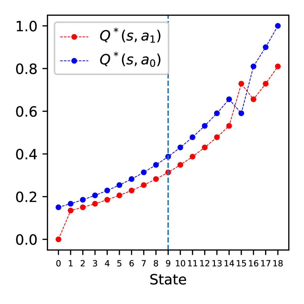
(a)

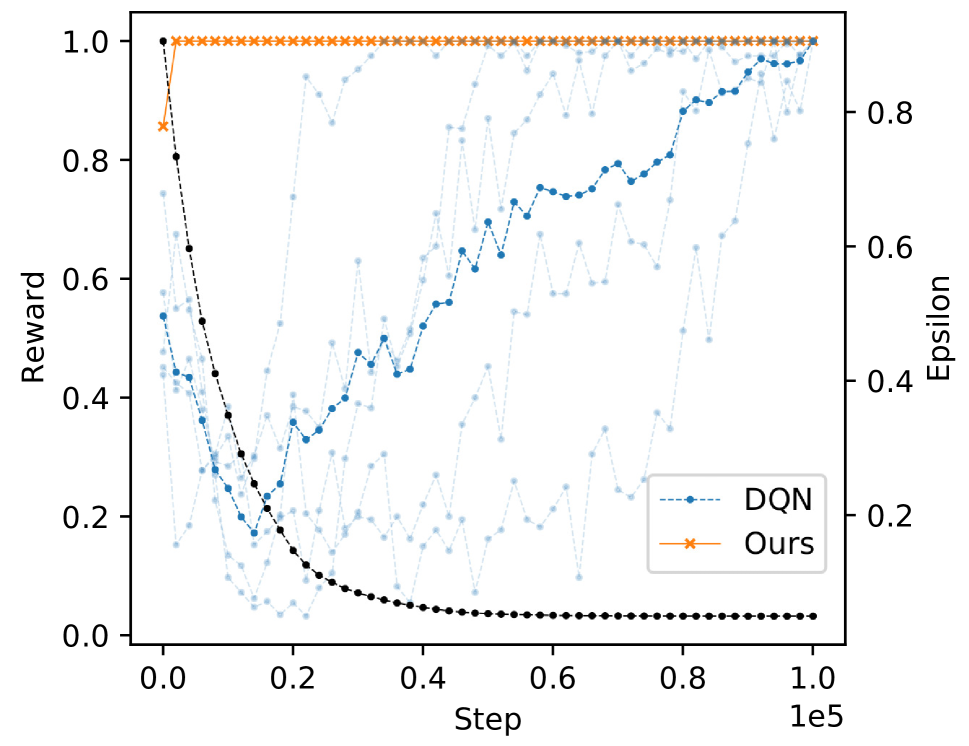
(b)

Figure 2: (a) Optimal Q-values for the Image Random Walk MDP (b) Performance on Image Random Walk over time. Exploration $\epsilon$ shown as black dotted line with scale on right axis.

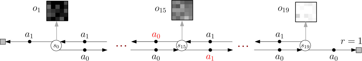
Figure 12: Transition diagram for the 19-state image random walk MDP. No reward is received except after taking $a_{1}$ in State 19. State 15 is a special state where the direction of actions is reversed. All transitions are deterministic. $\gamma=0.9$.

As a base environment, we first introduce a 19-state deterministic MDP with image observations and $\gamma=0.9$. The 19 states are arranged in a flat line, in order of index. At each state two actions are available, $a_{0}$ to the left, action $a_{1}$ to the right. State 15 is special, here the actions are reversed (i.e. $a_{0}$ moves to the right, action $a_{1}$ to the left). A transition diagram is included in the supplementary material (Fig. 12).

At all transitions the reward is zero, except for action $a_{0}$ from state 19, which yields a reward of 1. State 9 is the initial state. Observations for each state are noisy grayscale blocks, with the intensity corresponding to the states index $o_{i,j}=\mathcal{N}(n,\sigma),i,j\in\{1..D\},n\in\{1..19\}$ where D is the height and width of the observations and $n$ is the index of the state, normalized to a range of $[-1,1]$. We choose $D=5$ and $\sigma=0.1$. The optimal Q-functions for the system are shown in Fig 2(a), where it can be seen that simple policies such as “always move right” cannot succeed due to the action switching at State 15.

We also plot the reward (Fig 2(b)) obtained at the end of each episode for a tuned DQN agent and our approach. Both methods settle on the optimal policy, however our memory based approach learns almost immediately, whereas the DQN is still converging after 100k steps. This result highlights that in some cases it is simply much easier to store visited returns and generalise locally at inference time, as opposed to trying to fit a global value function.

4.2 ATARI100k

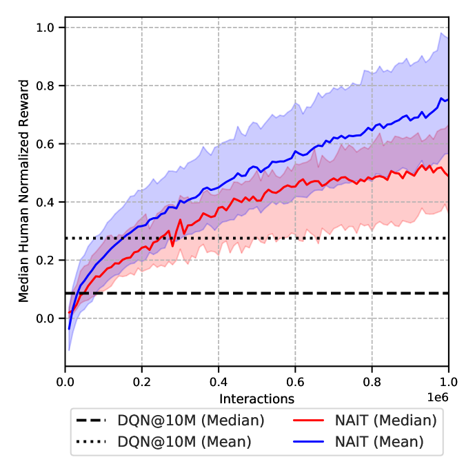
Figure 3: HNS over 1M interactions averaged over the full 57 ATARI game set. Shaded region indicates 90% confidence interval. DQN performance after 10M interactions is also shown, as comparable sample efficient methods do not evaluate on the full game set. NAIT requires only 150k interactions to outperform DQN@10M on both metrics.

		ATARI100K		All 57 Games
Method	Samples	Mdn	Mean	Mdn	Mean
Online (low budget)
SimPLe	100K	14.39	44.3	-	-
DE-R	100K	28.5	16.1	-	-
OT-R	100K	26.4	20.4	-	-
CURL	100K	17.5	38.1	-	-
DrQ	100K	28.42	35.7	-	-
SPR†	100K	41.5	70.4	-	-
NAIT	100K	31.21	36.23	17.57	36.51
Online (medium budget)
NAIT	250K	39.46	52.86	26.54	48.81
PPO	500K	20.93	43.74	-	-
NAIT	500K	46.73	69.97	43.63	66.46
NAIT	750K	60.64	79.38	50.05	73.26
NAIT	1M	60.60	90.38	52.04	82.81
SARSA‡	2M	35.85	72.40	28.27	57.75
DQN	2M	27.8	52.95	8.61	27.55
Unsup. Pretraining (250M budget) + Online Finetuning
VISR	100K	9.5	128.07	6.81	102.31
APT	100K	47.5	69.55	33.41	47.73
APS∗	100K	51.45	87.59	-

Table 1: Final performance measures. ^∗No shared encoder. ^†Data augmented. ^‡ SARSA($\lambda$) with Blob-PROST features.

ATARI100k was first introduced as a testbed for SimPLe (Kaiser 2019) and consists of 26 “easy exploration” ATARI2600 games. Since its introduction numerous works have focused solely on ATARI100k (van Hasselt, Hessel, and Aslanides 2019; Kielak 2020; Kostrikov, Yarats, and Fergus 2020; Srinivas, Laskin, and Abbeel 2020; Schwarzer et al. 2020). In our work, we report results for ATARI100k, but also evaluate on the 57 game set used more frequently in the wider RL literature. We do this both to provide a more robust baseline for future work, and to evaluate the generality of NAIT, as we do all hyperparameter tuning on the 26 game set alone, and make no changes when applying to the full evaluation suite. This setup was originally suggested by the ALE authors (Machado et al. 2018), and demonstrates that an approach is not overfitted to the task suit, however to date it has not been commonly adopted. We include a comparison to state-of-the-art sample efficient methods in Table 1. The unsupervised setting is included to contextualize NAIT’s high level of performance on the full 57 game set, however we do not evaluate NAIT in this setting. Full settings for ATARI are listed in the supplementary material.

We run all experiments with 10 seeds, and evaluation is done on a rolling basis following the recommendations of  (Machado et al. 2018), with the mean of the most recent 5 episodes logged for each seed. The DQN and SARSA($\lambda$) baselines are also reproduced from this work. Final scores are the mean score of 50 episodes, run after the completion of training, following (Schwarzer et al. 2020). Our main metric is the Human Normalized Score, $\textrm{HNS}=\frac{\text{agent}-\textrm{random}}{\text{human}-\textrm{random}}$ achieved within a fixed interaction budget. We primarily report the Median HNS (MHNS) across games as the mean tends to be dominated by outlier performance.

As speed is a major feature of NAIT, we log median iterations per second (itr/s) across games. Itr/s is calculated by dividing the time to complete the environment by 100k, averaged over ten seeds. Per-node speeds are the total throughput when all threads are allocated on a single AWS C5d.24xlarge (48 cores). This metric is indicative of real-world performance but is dependent on the number of cores present in the node. For this reason we also report per-thread speeds which are independent of core count but do not consider factors such as I/O blocking, although in practice we observe these effects to be minor. SPR, SimPLE and DE-Rainbow speeds in Table 2 are reproduced from (Schwarzer et al. 2020), with Dr Q and CURL and OT-Rainbow bench-marked from from open-source implementations running on P3.16xlarge (32 core, 8xP100 GPU) instances.

NAIT achieves a high level of performance, outperforming all methods with the exception of augmented SPR on the ATARI100K benchmark (see Table 1). This is achieved with a hugely reduced computational cost - over 100x faster than SPR and 1000x faster than SimPLe (see Table 2).

Algorithm	1 Node Itr/s	Walltime (hours)
SimPLe	0.5	3166.67
DE-R	53.4	29.65
OT-R	48.4	32.71
CURL	58.4	27.11
DrQ	15	105.56
SPR	9.25	171.17
SPR (augmented)	6.03	262.58
NAIT	13962.24	0.11

Table 2: Average single-node iterations/s and walltime required to complete the full 57 game for various methods on a single node.

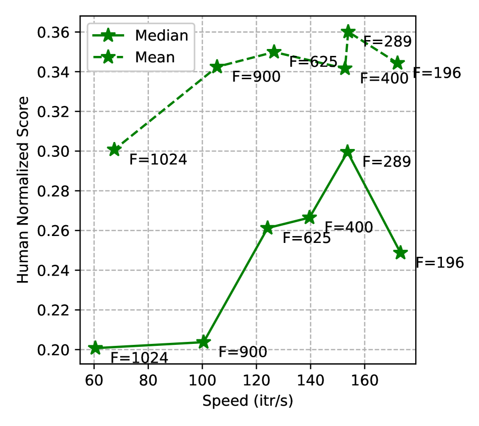
(a)

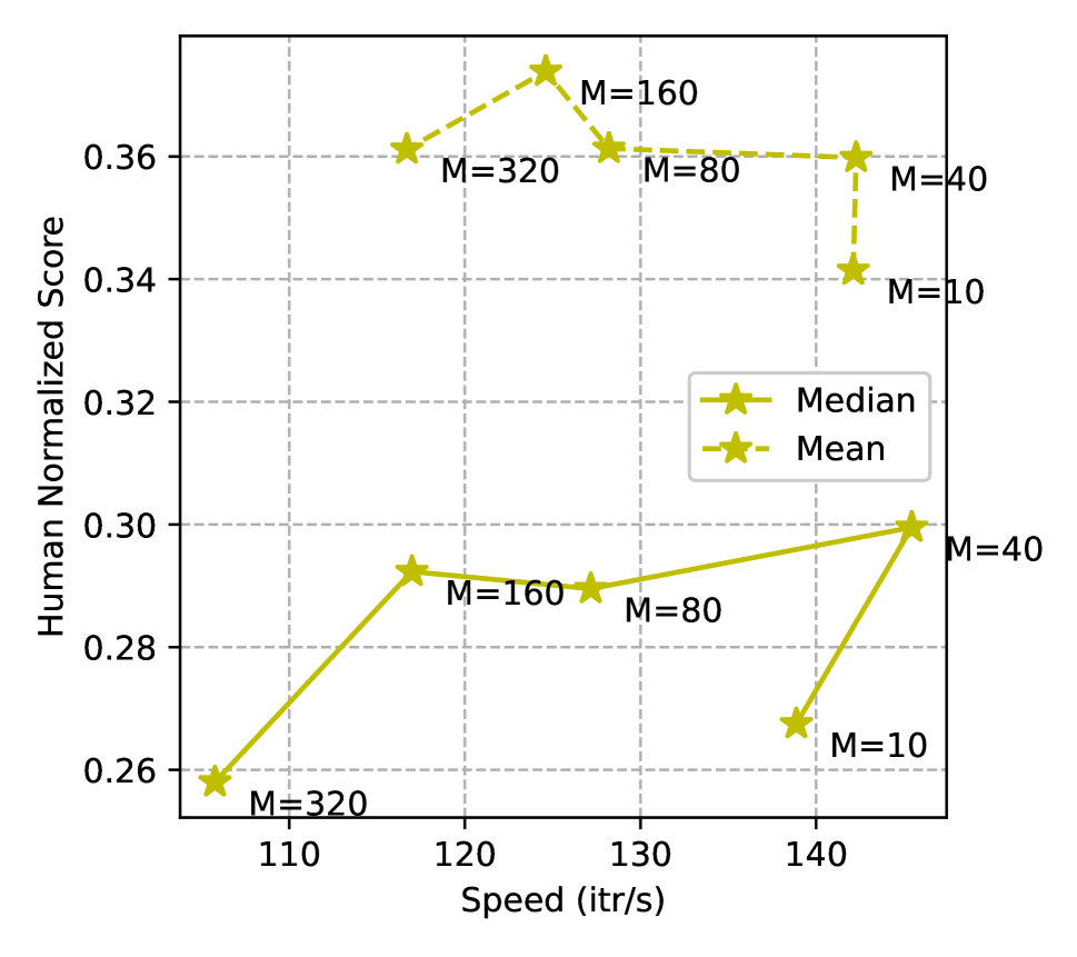
(b)

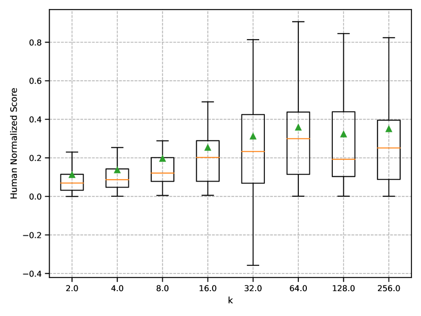
(c)

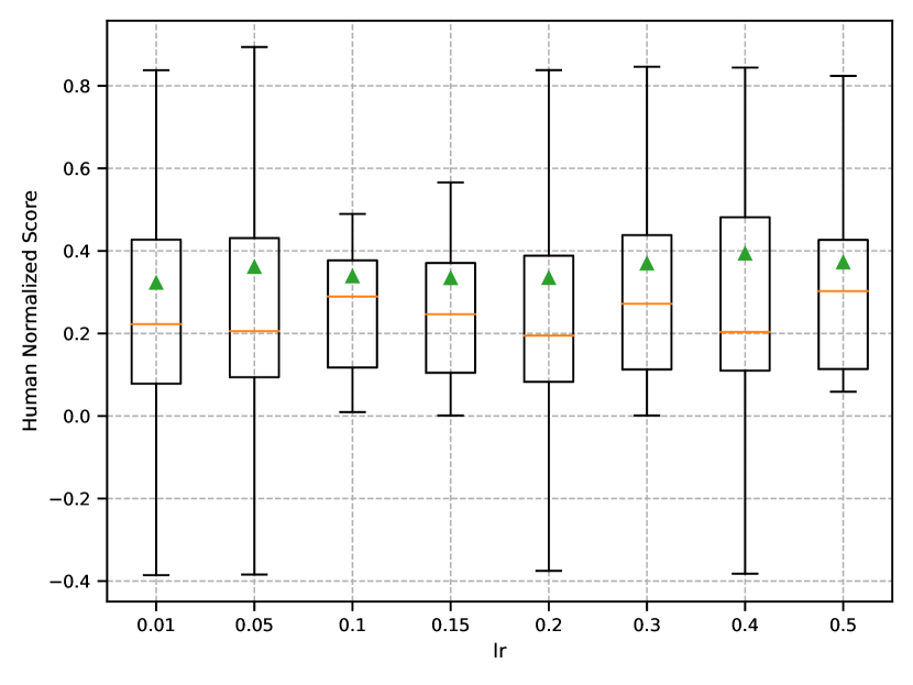
(d)

Figure 4: Sensitivity sweeps illustrating the sample efficiency (MHNS) and computational complexity (itr/s) trade-off by the choice of (a) projected dimension $F$ (b) $M$, which affects the speed/recall ratio of HNSW. Up and to the right is better. For parameters that do not affect speed, we plot the distribution of final HNS’s for c) $k$, and d) $\alpha$. Orange line indicates median, green diamond the mean. All game scores are first averaged over 10 seeds.

5 Analysis

5.1 Ongoing learning

NAIT demonstrates the high level of performance that a nonparametric approach can learn when environment interactions are limited. However, due to the fixed representation, NAIT’s performance will saturate once the importance of a good representation (i.e. non-local generalization) outweighs the importance of quickly updating the value function or policy. As stated, the 100k domain is of interest in its own right, however we are also interested in quantifying the point at which design choices such as a fixed representation begin to limit performance.

Using the same set of hyperparameters tuned for the ATARI100k benchmark (26 games, 100k interactions), we carried out a longer run over 1M interactions, and included all 57 games in the standard evaluation set (Fig. 3). We made no other alterations to NAIT or its hyperparameters. Learning is highly stable and indicates NAIT possesses a high level generality. Per-game performance during training is visualized in the supplementary material.

5.2 Ablations

Component	Replacement	MHNS	Itr/s
NAIT		31.2	163.4
DCT projection	Very sparse	21.5	121.3
DCT projection	Sparse	28.1	91.4
DCT projection	None	-	1.5
Tiebreaking	Uniform	12.1	125.3
Intertrace update	Monte-Carlo	13.6	141.2
Tricubic kernel	Mean	28.4	161.4
HNSW	KD tree	-	0.3

Table 3: Ablations. Median HNS and single-thread itr/s reported for the 26 game subset and 100K iterations.

When removing components, if a replacement is required, we choose what is either simplest or is already standard. For example, in place of a tricubic kernel, we use a uniform kernel, or instead of HNSW we use a KD-tree. Results are listed in Table 3.

We find that DCT components provide better quality representations with regard to performance and are faster to compute. Computation on the raw frames was prohibitively slow due to the resulting high dimensionality of the $k$-NN keys.

One unusual feature is the impact of distance based tiebreaking, in comparison to randomly breaking ties. This is likely because early in learning this encourages exploration based on novel states, as all estimates are zero, rather than simply ensuring a roughly uniform selection of actions. This is supported by the strong level of performance on the unseen ‘hard’ exploration games, despite no other mechanism of exploration being built into NAIT. Of lesser importance is the use of tricubic kernel which is shown to result in an increase in performance with only a small cost in computation speed in comparison to a uniform kernel (i.e. take the mean), however this increase is minor.

5.3 Effect of Hyperparamters

Higher representation dimension $F$ tends to be both slower, and perform worse as it is increased past $F=289$ (Figure 4). We hypothesise this is due to poorer recall of HNSW at higher dimensions overshadowing information preservation gained by a higher $F$. This could potentially be offset by increasing the recall of the lookup via the ef and M parameters, however this would come at the cost of a significant reduction in computational efficiency. Interestingly, as $F$ is held constant and M increased, performance is stable up to $M=160$, but drops sharply after this. This would indicate some level of noise in the value estimate is beneficial, and perfect recall is in fact not desirable for NAIT. Setting M too low however also degrades performance as expected.

Such high performance with low $F$ indicates that the information required to learn basic play is present in a surprisingly small number of DCT coefficients. One implication for ATARI100k is that learning a good representation is significantly less important in early learning than being able quickly assign credit.

From our sweeps, $k$ appears to have a clear optimal value across all games (see fig 4(a)). This is expected as $k$ effectively balances local generalization with the smoothness of the value estimate, and setting $k$ too large removes information from the value estimate. In contrast, the choice of learning rate does not effect performance smoothly, however the high-level metrics are surprisingly strong even at large $\alpha$, displaying a level of robustness to the choice of $\alpha$ that departs significantly from neural-based approaches. One explanation is due to $\alpha$ not being considered at new $(s,a)$ pairs where the new value is set directly. This forces NAIT into a high-learning rate setting by default.

6 Conclusion

We have introduced a locally generalising approach to RL that is both sample and computationally efficient, achieving state of the art performance in the low sample regime on ATARI while requiring two orders of magnitude less walltime. Due to the very low walltime and computational requirements, we hope that future work adopts our algorithm as a benchmark when demonstrating the efficacy of learned model or learned representation approaches. Further work may investigate the possibility of our approach as a quick but simple initial learner that can merge into, or inform, a more complex learner that does produce useful representations, via mechanisms such as behavioural cloning or similar. This has exciting potential to significantly improve the sample efficiency of established methods while maintaining their asymptotic performance.

Appendix A Implementation Details

A.1 ATARI

Throughout the literature it is common to observe slight alterations in the underlying environments used to benchmark approaches. This makes direct comparison difficult, and indeed among the current state-of the art approaches on the 100k domain the specifics of the ATARI setup do vary. We endeavored to choose parameters most similar to those recommended by the original authors, and not those that result in the maximum the raw score. Where our choices deviate (to facilitate comparison to previous methods), we run separate ablation studies with the recommended values (Fig. 5 and 6). NAIT is robust to changes in the underlying environments, with reward clipping having little effect and sticky actions resulting in a minor decrease in performance, which is expected as it makes control more challenging. Notably the change in HNS distribution between the 57 and 26 game sets is minor, indicating that NAIT has not been overfitted to the 26 game set.

Hyperparameter	Symbol	Value
Number of Neighbours	$k$	64
State Dimension	$F$	289
Discount	$\gamma$	0.99
Learning Rate	$\alpha$	0.1
HNSW settings
efc		200
efs		200
M		40
Space		$L^{2}$

Table 4: Default hyperparameters for NAIT.

Hyperparameter	Ours	D.E. Rainbow	SimPLe	SPR	Recommended
Greyscale	True	True	True	True	True
Observation size	(84, 84)	(84, 84)	(84, 84)	(84, 84)	(84, 84)
Interpolation	Inter-linear	Inter-linear	Inter-area	Inter-area	n.a.
Sticky Actions	False	False	False	False	True
Frameskip/Action Repeat	4	4	4	4	n.a.
Framepooling	True	True	True	True	n.a.
Colour Averaging	False	False	False	False	n.a.
Framestack	4	4	4	4	n.a.
Terminal on loss of life	False	True	False	False	False
Reward Clipping	False	True	True	True	False
Max No-Op Starts	30	30	n.a.	30	0
Seeds	10	5	10	10	n.a.
Max frames	400k	400k	400k	400k	n.a.

Table 5: ATARI100k evaluation settings for various approaches. Recommended is from Machado et. al. 2018.

A.2 NAIT

Exact match lookups are computed efficiently via a hashtable. For fast hashing, we make use of the Extremely Fast Non-Cryptographic Hash library xxhash, available at https://github.com/Cyan4973/xxHash. To keep the memory overhead low, we initialize all buffers with a fixed capacity of 1000 samples, and double their capacity when filled. Because no representation learning is carried out, our approach does not require a significant number of hyper-parameters to be tuned. The final values are listed in Table 4. Note that HNSW parameters do noticeably effect performance, as they determine the recall of the approximate neighbour lookup.

A.3 HNSW

HNSW was chosen as the approximate nearest neighbour library as presents the best speed/recall performance on dense data at the time of publication. There are several implementations available; we make use of v0.5.0 of the header-only library available at https://github.com/nmslib/hnswlib. While there are some feature restrictions, this implementation supports incremental index construction (i.e. single data points can be added without requiring re-indexing), which is critical to our approach. HNSW’s speed/recall tradeoff can be can be significantly altered via three parameters; efs, efc and M. efs is the size of the candidate list to keep during search - in general larger efs leads to higher recall but slower lookups. efc is the same parameter as efs, but refers to the value during construction time, when a new point is being inserted. M determines the number of bi-directional links made for each node when constructing the proximity graph. Higher values also correspond to higher recalls at the cost of speed, and M also directly effects the memory requirements of the index.

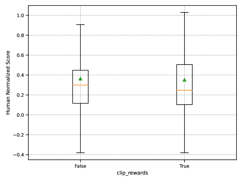
Figure 5: Effect of reward clipping on NAIT on ATARI100k.

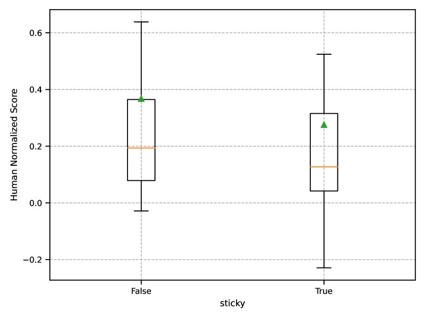
Figure 6: Effect of sticky actions on NAIT’s performance over the entire 57 game set. Stochastic max 30 no-ops enabled for both True and False.

To quantify the effect of efs and efc on performance, we sampled 10000 frames from each game (with a random policy), applied the DCT transform with $F=225$ and calculated the recall for a query of $k=30$ neighbours for 1000 samples, over a range of values, averaging the result. Fig. 14 displays the outcome. In general recalls are surprisingly high, even for low values of efs and efc, however the general trend is as expected, with higher values leading to increases in recall, but decreases in speed. Due to the high recall present in all runs, it is clear that inaccuracies in the value function due to poor lookup results will be minor for most games.

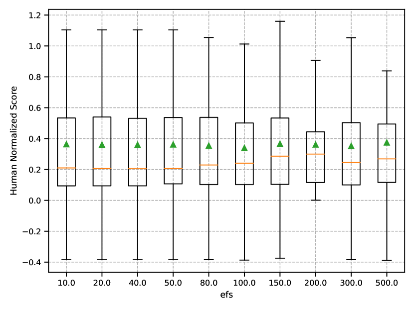
Figure 7: HNS distribution fine-grained sweep of HSNW parameter efs on ATARI100k

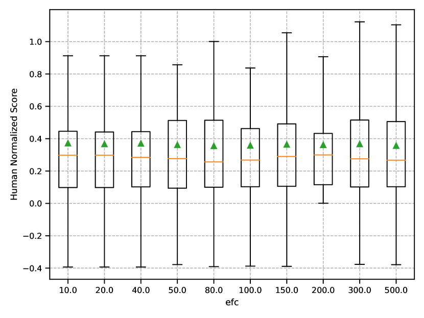
Figure 8: HNS distribution fine-grained sweep of HSNW parameter efc on ATARI100k

In addition to quantifying the recall on random policy frames, we also carried out full benchmark sweeps over the efs and efc parameters. Higher efs tends to increase performance which is expected, however it does appear to have an optimal point. We hypothesise that a small error in recall may actually be desirable as it provides a mechanism for exploration, which we do not have explicitly builtin except in the case of a tiebreak. As the number of samples grows, the effect of poorer recall on value estimates is reduced (as an area becomes more densely covered), leading to a scheme similar to e-greedy on a decaying schedule.

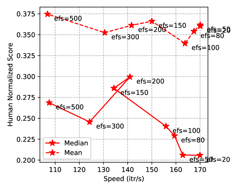
Figure 9: Speed-Performance curve of efs on ATARI100k.

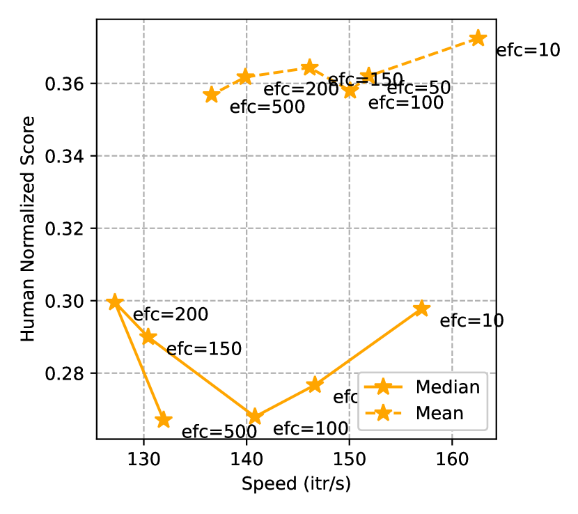
Figure 10: Speed-Performance curve of efc on ATARI100k.

Appendix B Further Analysis: Walltime

The benefit of lower computational complexity is limited in many applications if it comes with a proportional decrease in sample efficiency. In ATARI for example, if NAIT runs twice as fast, but takes double the number of samples to meet the performance of competing methods, it’s benefit is questionable. Here we make the comparison as explicit as possible and plot performance against walltime for a single representative game, ‘Ms Pacman’ (‘Ms Pacman’ was chosen as it is often the ‘median game’ in our experiments). We baseline against SPR - the current state of the art for sample efficiency. Note that NAIT runs in a single thread, while SPR requires multiple threads and access to a P100 GPU. We perform 10 separate runs and plot them on top of each other, performing no averaging or interpolation, logging the trailing 5-episode reward every 1000 interactions. We run NAIT for 250k steps. It takes NAIT $8$ minutes to achieve the performance of SPR@100k samples (which takes SPR 4.6 hours).

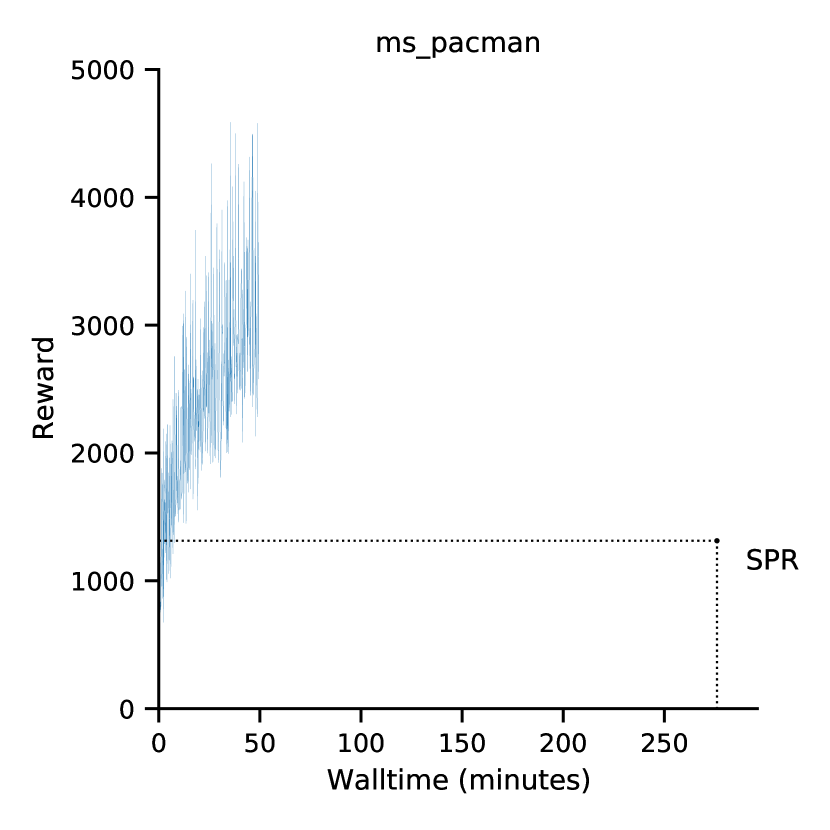
Figure 11: Raw score as a function of walltime for ‘median’ game Ms Pacman.

Appendix C Further Discussion

C.1 Importance of Adaptive Kernel Interpolation

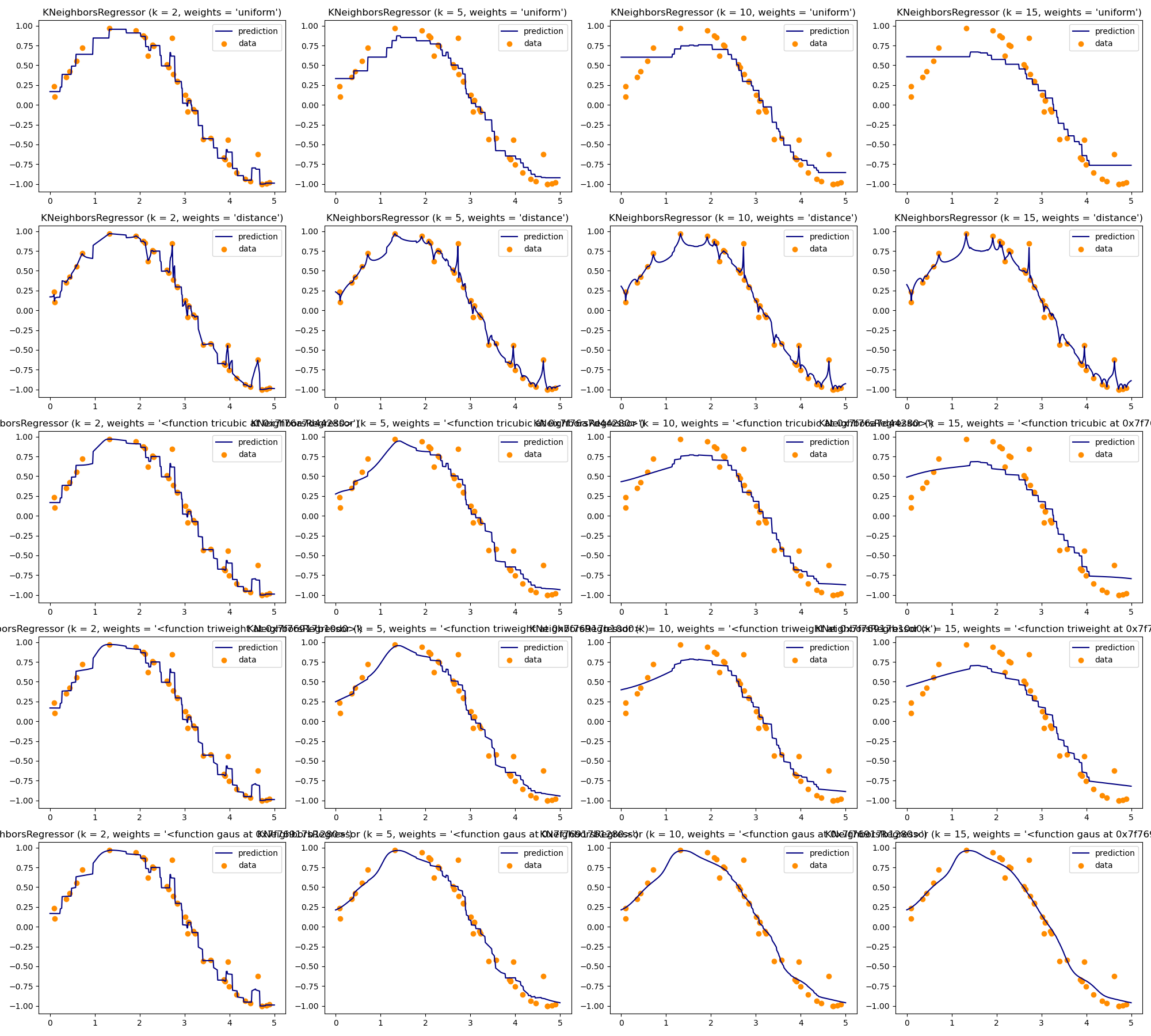
Figure 15: Visualization of kernel type and $k$ on 1D interpolation quality. Rows represent a uniform, inverse distance, Tricubic, Triweight, and Gaussian kernel respectively, with columns indicating increasing $k$. Triweight and Tricubic can be seen to be highly dependent on $k$ for their quality, but provide broad generalization when the data is sparse (see the peaks in rows 3 and 4 of column 2), and behave similarly to a mean when the data is dense.

The use of an adaptive kernel (i.e. one which does not require a fixed bandwidth hyperparameter) is important as the absolute distances between state representations will vary from game to game (as a function of how much pixel intensity varies). In addition, the type of smoothing applied by the kernel can have a significant effect on the final Q-value approximation. Inverse distance weighting, for example, which has been used in other work, creates a distinct “spiky appearance” which becomes more pronounced in higher dimensions as the space between samples grows. Under this interpolation very sharp changes in the value function can occur as one approaches an already sampled point, which is undesirable. Gaussian kernels in general produce the most appealing-looking estimates, but come with the aforementioned drawback of requiring a fixed bandwidth set at the start of training for all games. Normalized tricubic kernels provide a good compromise - however as can be seen their performance is highly dependent on $k$, hence the importance of its value in our overall algorithm. For emphasis, theses effects are visualized in Fig. 15 on sample 1D data.

C.2 Benefits of a DCT over Random Projection

One surprising result in our work is the out-performance of random projection-based representations by a DCT-based representation. We hypothesize two main reasons for this;

1. Bias towards global representation because we select DCT components in decreasing order of frequency, we bias towards large, global representations of the current game state. Tuning $F$ in this scenario modifies the level of granularity that is preserved in the representation. Low $F$ captures only broad gradients and shapes, while high $F$ captures greater detail but comes with the discussed downstream costs. By tuning $F$ we allow the algorithm to capture sufficient low-level detail (such as the location of the ball in pong) to facilitate basic play, but nothing more.

2. DCT coordinates are normalized. Because DCT coordinates are already normalized no dimension is weighted higher than any other in the $k$-NN lookup. In contrast, if a random projection is used, one of the random bases may by chance cover pixels that have much higher average intensities than another. In this case, it will be weighted higher in the subsequent lookup as that dimension is “stretched” proportional to the intensity increase. This is a common problem when using $k$-NN lookups and is remedied by normalizing all dimensions to the same range. This is not possible in our case as the ranges of each dimensions are not known before learning begins. In this scenario and adaptive normalization scheme, that tracks running statistics over each dimension and normalizes accordingly, may be necessary.

In regards to compute efficiency, the DCT is also faster than a standard projection. This is due to the highly optimized underlying fft libraries used to compute the DCT (scipy.fftpack), which run in $\mathcal{O}(DlogD)$, vs $\mathcal{O}(DF)$ for the random projection.

C.3 Why Does a Nonparametric Approach Perform so Well on ATARI100K?

A major advantage to ATARI100k is that because samples are limited, no forced forgetting is required to ensure memory limits are not exceeded, as the entire game history is less than the size of a standard replay buffer. However, given that our representation is quite naive, a better question is perhaps why value-function methods perform so poorly. We discuss several possibilities below.

Value function approaches to Deep-RL learn a Q-function

$$Q^{\pi}_{\theta}(s,a)=\mathbb{E}_{\pi}\left[G_{t}|s_{t}=s,a_{t}=a\right]$$ (12)

from which a policy is derived, most commonly $\epsilon$-greedy (Chung et al. 2015), although transformations via softmax and related operators are also used (Song, Parr, and Carin 2019). The Q-function is parameterised (indicated via subscript) by a DNN. Initial attempts (Riedmiller 2005) to combine neural function approximation with Q-learning minimised the squared one-step TD error calculated on stored samples,

$$\mathcal{L_{\text{DQL}}}=\left(Q^{\pi}_{\theta}(s,a)-\left(r_{t}+\gamma\max_{a}Q^{\pi}_{\theta}(s^{\prime},a^{\prime})\right)\right)^{2}.$$ (13)

While this appears a reasonable generalisation of tabular Q-learning to high-dim observations, it is unstable and in most cases will not converge. This is due to the combination of function approximation, bootstrapping, and off policy training commonly known as the deadly triad (Tsitsiklis and Van Roy 1997). Bootstrapping and function approximation are particularly damaging when the approximation is poor, as errors are immediately propagated, requiring low learning rates to avoid divergence. This limitation is highly pronounced in the low-sample domain, where any parameterization will be poor if initialized randomly.

Another explanation is the method by which samples are incorporated. In general, for sample efficient learning we want to store and exploit raw information about the environment to the greatest extent possible as interactions are the constraining factor. Experience replay does store raw experiences (although if n-step returns are used they become policy dependent), but traditional approaches do not fully exploit this information. This is due to the under-use of available data due to limited training steps performed on the value network combined with the necessity of low learning rates. As a consequence, all available information is not fully incorporated into the Q-function approximation early during training. The original DQN for example, uses 4 interactions with the environment for each training step. SPR, in contrast, uses the highest published ratio of 2 training steps per interaction with the environment, and in ablation studies showed increasing this parameter significantly improves sample efficiency. However even if all samples in the buffer are sampled at some point for training (which is unlikely), due to the low learning rate their information will still not be fully incorporated into the Q-function parameterization.

C.4 Effect of the Discount Rate

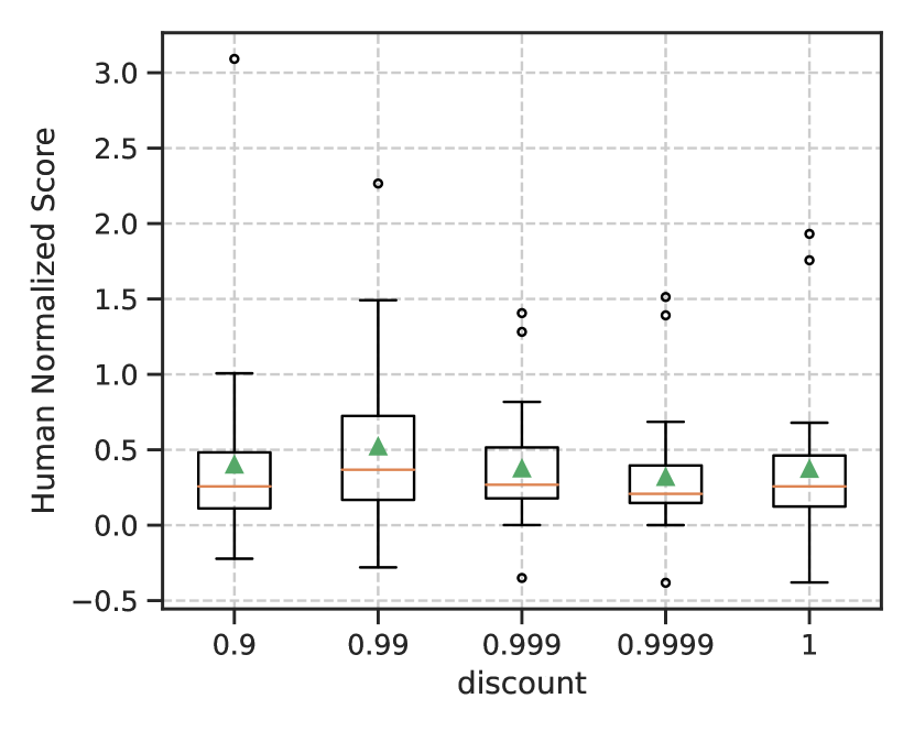
Figure 13: Effect of $\gamma$ on total HNS on ATARI100k

The actual objective being optimised is total reward, and so to maximise directly what we care about, $\gamma=1$ would seem appropriate. As others have noted, however (Schulman et al. 2018), often a surrogate objective created by a lower discount rate can produce better results. We observe this phenomenon here, with the optimal discount found to be 0.99, lower than is traditional. This is likely due to the much shorter trace lengths that occur when the interaction budget is limited (as the agent does not reach superhuman levels of play that result in large game lengths).

Figure 13 shows the effect of various discount rates on HNS over time. Interestingly, we observe for some games a clear demarcation in performance induced by a varied $\gamma$. This is most pronounced in the game freeway, where higher discounting significantly improves final performance. For freeway, this is likely caused as low discounting results in the agent repeating the first route it finds to the “goal” (crossing the street), regardless of its efficiency. More aggressive discounting directly pushes the agent towards short paths, which allows it to reach a higher final score within the time-limit.

Figure 14: Runtime/Recall tradeoff of HNSW parameters ef and efc for each game. Up and to the left is best.

Game	Random	Human	100K	250k	500k	750k	1M
Alien*	227.8	7127.7	918.35	1072.5	1433.3	1836.8	2057.2
Amidar*	5.8	1719.5	213.37	377.065	481.875	592.225	715.96
Assault*	222.4	742	483.21	509.145	524.685	537.495	537.285
Asterix*	210	8503.3	900.5	1336.25	1920.75	2678	3294.5
Asteroids	719.1	47388.7	606.15	982.55	1134.75	1261.7	1431.55
Atlantis	12850	29028.1	32268.5	45540.5	57116.5	79494	83677.5
Bank Heist*	14.2	753.1	98.3	143	176.25	197.2	204.55
Battle Zone*	2360	37187.5	9595	9930	12110	14250	14675
Beam Rider	363.9	16826.5	622.7	655.48	764.86	856.54	857.42
Berzerk	123.7	2630.4	564.2	789.1	882.15	893.95	911.1
Bowling	23.1	160.7	74.01	86.435	86.325	90.47	91.09
Boxing*	0.1	12.1	5.135	10.97	15.44	18.57	24.4
Breakout*	1.7	30.5	11.665	18.865	40.815	37.6	48.025
Centipede	2090.9	12017.1	5369.32	7076.52	10295.98	11805.91	12440.17
Chopper Command*	811	7387.8	1711	2368	2592	4158	3893
Crazy Climber*	10780.5	35829.4	1240.5	3147	6092	7908	8506.5
Defender	2874.5	18688.9	4451	6540.5	8706.5	9700.75	11655.5
Demon Attack*	152.1	1971	262.025	332	389.275	458.175	458.175
Double Dunk	-18.6	-16.4	-5.39	-6.6	-3.07	-6.63	-5.99
Enduro	0	860.5	4.345	4.715	8.95	12.325	17.44
Fishing Derby	-91.7	-38.7	-80.92	-74.035	-68.575	-62.67	-58.325
Freeway*	0	29.6	25.09	25.865	26.1	26.04	26.075
Frostbite*	65.2	4334.7	1808.8	2783.85	3610.8	4029.3	4462.6
Gopher*	257.6	2412.5	979	1528.9	2597.5	2701.9	4315.7
Gravitar	173	3351.4	451	594.75	727.75	828	909
Hero*	1027	30826.4	5311.2	5524.25	5538.225	5573.275	5576.875
Ice Hockey	-11.2	0.9	-8.965	-7.97	-5.91	-5.08	-4.65
Jamesbond*	29	302.8	306.25	418.5	482.25	499.5	496.75
Kangaroo*	52	3035	983	1229	1818.5	1915	2038.5
Krull*	1598	2665.5	3588.64	3851.905	4227.73	4570.51	4733.92
Kung Fu Master*	258.5	22736.3	10408	17178	24448	26809.5	30329.5
Montezuma Revenge	0	4753.3	0	0	0	35	80
Ms Pacman*	307.3	6951.6	2579.2	2951.15	3412.45	3654.1	3764.7
Name This Game	2292.3	8049	3522.05	4196.75	5241.4	5173.55	5914.9
Phoenix	761.4	7242.6	1448.3	2467.9	3729.45	4563.8	4852.5
Pitfall	-229.4	6463.7	-166.855	-29.79	-198.64	-77.075	-3.015
Pong*	-20.7	14.6	-7.89	2.76	12.27	14.6	15.225
Private Eye*	24.9	69571.3	105.38	-153.495	-209.215	-88.195	-54.48
Qbert*	163.9	13455	2361.125	4475.125	6273.75	8291.375	9557
Riverraid	1338.5	17118	2634.95	3615.65	4409.35	5061.2	5247.3
Road Runner*	11.5	7845	7113.5	12953.5	14113	16166	17408
Robotank	2.2	11.9	4.905	4.89	5.845	5.425	6.395
Seaquest*	68.4	42054.7	417.1	596.9	778.2	830.4	927.7
Skiing	-17098.1	-4336.9	-30372.155	-30623.19	-30664.61	-30901.3	-30696.87
Solaris	1236.3	12326.7	967.3	1381.9	1788.4	1750.2	2622.5
Space Invaders	148	1668.7	646.125	999.225	1289.825	1304.5	1428.325
Star Gunner	664	10250	1324.5	1401	1400	1386.5	1347
Tennis	-23.8	-8.3	-4.89	-5.855	-6.96	-5.735	-5.605
Time Pilot	3568	5229.2	2821.5	3284.5	4161.5	5159	5646.5
Tutankham	11.4	167.6	99.68	111.31	104.535	78.54	81.63
Up N Down*	533.4	11693.2	7657.75	12082.95	18006.6	22985.4	27364.05
Venture	0	1187.5	129	283.5	495	481.5	582.5
Video Pinball	0	17667.9	5901.24	7280.085	9682.72	12524.755	12422.07
Wizard OfWor	563.5	4756.5	1041	1353	3337	4234	6451.5
Yars Revenge	3092.9	54576.9	6015.505	7973.015	8920.34	11150.245	12841.105
Zaxxon	32.5	9173.3	2818.5	4850.5	6339.5	7081	7864.5
ATARI100K Mean HNS			0.362	0.529	0.700	0.794	0.904
ATARI 100k Median HNS			0.312	0.395	0.467	0.606	0.606
Mean HNS			0.365	0.488	0.665	0.733	0.828
Median HNS			0.176	0.265	0.436	0.501	0.520

Table 6: Full numerical results for NAIT. HNS is Human Normalized Score, equal to $\frac{\text{agent}-\text{random}}{\text{human}-\text{random}}$. For our results, at the completion of training, 50 episodes are run for 10 seeds over each game, with the final number averaged first over episodes, then over seeds. ^∗ Indicates the game belongs to the ATARI100k subset.

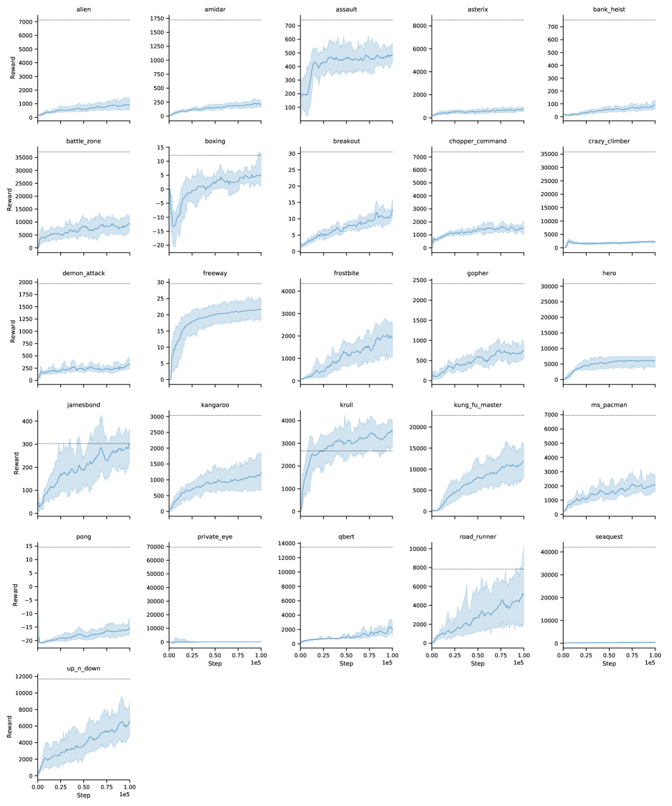
Figure 16: Game-by-game performance over 100k interactions for the 26 game ‘ATARI100K’ subset. Plots show trailing 5 episode average reward logged every 1000 interactions. Centre line is mean over 10 seeds, shaded area indicates the 90% confidence interval. Human Expert Score is indicated by horizontal black line.

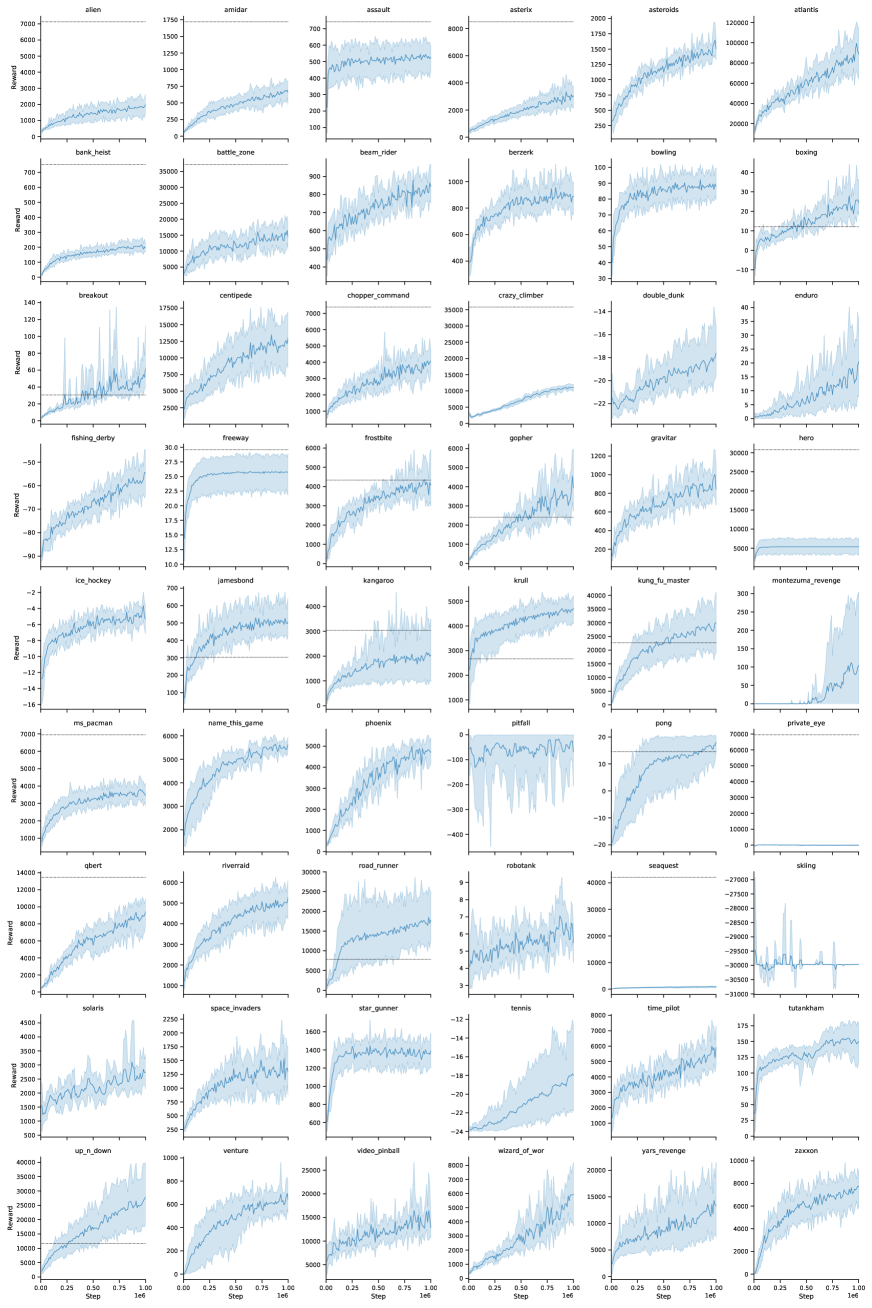
Figure 17: Game-by-game performance over 1M interactions for all games with hyperparameters tuned for the 26-game subset at 100k. Plots show trailing 5 episode average reward logged every 5000 interactions. Centre line is mean over 10 seeds, shaded area indicates the 90% confidence interval. Human Expert Score is indicated by horizontal black line on the 26 game subset.

References

- hns (2021) 2021. HNSWLib: https://github.com/nmslib/hnswlib.
- Achlioptas (2003) Achlioptas, D. 2003. Database-friendly random projections. In Journal of Computer and System Sciences, volume 66, 671–687.
- Aumüller, Bernhardsson, and Faithfull (2020) Aumüller, M.; Bernhardsson, E.; and Faithfull, A. 2020. ANN-benchmarks. Information Systems, 87: 101374.
- Badia and Piot (2020) Badia, A. P.; and Piot, B. 2020. Agent57: Outperforming the atari human benchmark. arXiv preprint arXiv:2003.13350.
- Bellemare et al. (2015) Bellemare, M. G.; Naddaf, Y.; Veness, J.; and Bowling, M. 2015. The arcade learning environment: An evaluation platform for general agents. In IJCAI, volume 2015-Janua, 4148–4152. ISBN 9781577357384.
- Bentley (1975) Bentley, J. L. 1975. Multidimensional binary search trees used for associative searching. Communications of the ACM, 18(9): 509–517.
- Berariu and Gogianu (2017) Berariu, T.; and Gogianu, F. 2017. Random Projection Based Representations for Learning Policies in Deterministic Atari Games. In CSCS, 233–238. ISBN 9781538618394.
- Blundell et al. (2016) Blundell, C.; Uria, B.; Pritzel, A.; Li, Y.; Ruderman, A.; Leibo, J. Z.; Rae, J.; Wierstra, D.; and Hassabis, D. 2016. Model-Free Episodic Control. arXiv:1606.04460v1.
- Cho et al. (2019) Cho, H.; Oh, P.; Park, J.; Jung, W.; and Lee, J. 2019. Fa3c: Fpga-accelerated deep reinforcement learning. In Proceedings of the Twenty-Fourth International Conference on Architectural Support for Programming Languages and Operating Systems, 499–513.
- Chung et al. (2015) Chung, J.; Gulcehre, C.; Cho, K.; and Bengio, Y. 2015. Gated feedback recurrent neural networks. Proceedings of the 32nd International Conference on Machine Learning, 37: 2067–2075.
- Dalton, Frosio, and Garland (2019) Dalton, S.; Frosio, I.; and Garland, M. 2019. Accelerating reinforcement learning through gpu atari emulation. arXiv preprint arXiv:1907.08467.
- Hafner et al. (2019) Hafner, D.; Lillicrap, T.; Ba, J.; and Norouzi, M. 2019. Dream to control: Learning behaviors by latent imagination. arXiv preprint arXiv:1912.01603.
- Hansen et al. (2019) Hansen, S.; Dabney, W.; Barreto, A.; Van de Wiele, T.; Warde-Farley, D.; and Mnih, V. 2019. Fast task inference with variational intrinsic successor features. arXiv preprint arXiv:1906.05030.
- Henderson et al. (2018) Henderson, P.; Islam, R.; Bachman, P.; Pineau, J.; Precup, D.; and Meger, D. 2018. Deep reinforcement learning that matters. In Proceedings of the AAAI conference on artificial intelligence, volume 32.
- Hessel et al. (2018) Hessel, M.; Modayil, J.; Van Hasselt, H.; Schaul, T.; Ostrovski, G.; Dabney, W.; Horgan, D.; Piot, B.; Azar, M.; and Silver, D. 2018. Rainbow: Combining improvements in deep reinforcement learning. In AAAI, 3215–3222.
- Kaiser (2019) Kaiser, L. e. a. 2019. Model-Based Reinforcement Learning for Atari.
- Kielak (2020) Kielak, K. 2020. Importance of using appropriate baselines for evaluation of data-efficiency in deep reinforcement learning for Atari. arXiv:2003.10181.
- Kostrikov, Yarats, and Fergus (2020) Kostrikov, I.; Yarats, D.; and Fergus, R. 2020. Image Augmentation Is All You Need: Regularizing Deep Reinforcement Learning from Pixels. arXiv:2004.13649.
- Laskin et al. (2020) Laskin, M.; Lee, K.; Stooke, A.; Pinto, L.; Abbeel, P.; and Srinivas, A. 2020. Reinforcement Learning with Augmented Data. arXiv preprint arXiv:2004.14990.
- Li, Hastie, and Church (2006) Li, P.; Hastie, T. J.; and Church, K. W. 2006. Very sparse random projections. In SIGKDD, volume 2006, 287–296. ISBN 1595933395.
- Li (2017) Li, Y. 2017. Deep Reinforcement Learning: An Overview.
- Liang et al. (2016) Liang, Y.; Machado, M. C.; Talvitie, E.; and Bowling, M. 2016. State of the Art Control of Atari Games Using Shallow Reinforcement Learning. In Proceedings of the 2016 International Conference on Autonomous Agents & Multiagent Systems, 485–493.
- Liu and Abbeel (2021) Liu, H.; and Abbeel, P. 2021. Behavior from the void: Unsupervised active pre-training. arXiv preprint arXiv:2103.04551.
- Machado et al. (2018) Machado, M. C.; Bellemare, M. G.; Talvitie, E.; Veness, J.; Hausknecht, M.; and Bowling, M. 2018. Revisiting the arcade learning environment: Evaluation protocols and open problems for general agents. JAIR.
- Malkov and Yashunin (2018) Malkov, Y. A.; and Yashunin, D. A. 2018. Efficient and robust approximate nearest neighbor search using Hierarchical Navigable Small World graphs. IEEE Transactions on Pattern Analysis and Machine Intelligence, 1–1.
- OpenAI (2019) OpenAI. 2019. Dota 2 with Large Scale Deep Reinforcement Learning. arXiv.
- Riedmiller (2005) Riedmiller, M. 2005. Neural fitted Q iteration–first experiences with a data efficient neural reinforcement learning method. In European Conference on Machine Learning, 317–328. Springer.
- Schulman et al. (2018) Schulman, J.; Moritz, P.; Levine, S.; Jordan, M.; and Abbeel, P. 2018. High-Dimensional Continuous Control Using Generalized Advantage Estimation. arXiv:1506.02438.
- Schulman et al. (2017) Schulman, J.; Wolski, F.; Dhariwal, P.; Radford, A.; and Klimov, O. 2017. Proximal policy optimization algorithms. arXiv:1707.06347.
- Schwarzer et al. (2020) Schwarzer, M.; Anand, A.; Goel, R.; Hjelm, R. D.; Courville, A.; and Bachman, P. 2020. Data-efficient reinforcement learning with momentum predictive representations. arXiv:2007.05929.
- Song, Parr, and Carin (2019) Song, Z.; Parr, R.; and Carin, L. 2019. Revisiting the softmax bellman operator. In ICML.
- Srinivas, Laskin, and Abbeel (2020) Srinivas, A.; Laskin, M.; and Abbeel, P. 2020. CURL: Contrastive Unsupervised Representations for Reinforcement Learning. arXiv:2004.04136.
- Stooke and Abbeel (2018) Stooke, A.; and Abbeel, P. 2018. Accelerated methods for deep reinforcement learning. arXiv preprint arXiv:1803.02811.
- Sutton (1990) Sutton, R. S. 1990. Integrated Architectures for Learning, Planning, and Reacting Based on Approximating Dynamic Programming. In Machine Learning Proceedings. Elsevier.
- Sutton and Barto (1998) Sutton, R. S.; and Barto, A. G. 1998. Introduction to Reinforcement Learning. Cambridge, MA, USA: MIT Press, 1st edition. ISBN 0262193981.
- Tsitsiklis and Van Roy (1997) Tsitsiklis, J. N.; and Van Roy, B. 1997. An analysis of temporal-difference learning with function approximation. IEEE Transactions on Automatic Control, 42(5): 674–690.
- van Hasselt, Hessel, and Aslanides (2019) van Hasselt, H.; Hessel, M.; and Aslanides, J. 2019. When to use parametric models in reinforcement learning?
- Wagner et al. (2010) Wagner, D.; Reitmayr, G.; Mulloni, A.; Drummond, T.; and Schmalstieg, D. 2010. Real-Time Detection and Tracking for Augmented Reality on Mobile Phones. IEEE Transactions on Visualization and Computer Graphics, 16(3): 355–368.