Simultaneous perturbation stochastic approximation: towards one-measurement per iteration

Abstract

When measuring the value of a function to be minimized is not only expensive but also with noise, the popular simultaneous perturbation stochastic approximation (SPSA) algorithm requires only two function values in each iteration. In this paper, we propose a method requiring only one function measurement value per iteration in the average sense. We prove the strong convergence and asymptotic normality of the new algorithm. Experimental results show the effectiveness and potential of our algorithm.

1 Introduction

We consider the following unconstrained optimization:

$$({\rm P})~{}~{}\min_{x\in\mathbb{R}^{n}}~{}f(x),$$

where $f(x):\mathbb{R}^{n}\to\mathbb{R}$ is differentiable with the noisy measurements and $g(x)$ is the true gradient. In order to iteratively solve (P), stochastic approximation (SA) is a popular algorithm scheme given by

$$\hat{x}_{k+1}=\hat{x}_{k}-a_{k}d_{k},$$

where $\hat{x}_{k}$ is an estimation of the feasible solution at $k$-th iteration, $a_{k}\in\mathbb{R}$ is a step size and $d_{k}\in\mathbb{R}^{n}$ is a iterative direction.

If the gradient of the function is noisily available, by setting $d_{k}$ as the noisy measurement of $g(x_{k})$, which is given by

$$\widetilde{g}_{k}=g(x_{k})+\varepsilon_{k},$$

where $\varepsilon_{k}$ is the noise of the gradient of the $k$-th iteration, SA reduces to the Robbins-Monro (RM) algorithm RM1951SA .

When the gradient is not available, the corresponding choice of the direction $d_{k}$ becomes an approximation of the gradient. Kiefer and Wolfowitz KW1952 proposed the finite difference stochastic approximation (FDSA) algorithm (also known as KW algorithm), which approximates $g(x)$ with the finite difference form $\hat{g}(x)$. That is, the $i$-th component of $\hat{g}(x_{k})$ is given by

$$\hat{g}_{i}(x_{k})=\frac{\widetilde{f}(x_{k}+c_{k}e_{i})-\widetilde{f}(x_{k}-c_{k}e_{i})}{2c_{k}},$$

where $\widetilde{f}(\cdot)$ is the measurement of $f(\cdot)$ with noise, $e_{i}$ is $i$-th column of the identity matrix and $c_{k}$ is a positive scalar. FDSA algorithm needs $2n$ measurements of the function value in order to approximate a gradient vector. Kushner and Clark 1978Stochastic proposed the random direction stochastic approximation (RDSA) algorithm, which only requires two measurements to approximate $g(x)$:

$$\hat{g}(x_{k})=\frac{\widetilde{f}(x_{k}+c_{k}\xi_{k})-\widetilde{f}(x_{k}-c_{k}\xi_{k})}{2c_{k}}\xi_{k},$$

where $\xi_{k}$ is a random vector satisfying some specific distribution. Spall spall1992 proposed the simultaneous perturbation stochastic approximation (SPSA) method based on the following approximation

$$\hat{g}(x_{k})=\frac{\widetilde{f}(x_{k}+c_{k}\xi_{k})-\widetilde{f}(x_{k}-c_{k}\xi_{k})}{2c_{k}}\xi^{-1}_{k},$$ (1)

where $\xi^{-1}_{k}$ takes the inverse of every element of $\xi_{k}$, $c_{k}$ is a positive scalar, and

$$\widetilde{f}(x_{k}+c_{k}\xi_{k}) =f(x_{k}+c_{k}\xi_{k})+\varepsilon_{k}^{+},$$

$$\widetilde{f}(x_{k}-c_{k}\xi_{k}) =f(x_{k}-c_{k}\xi_{k})+\varepsilon_{k}^{-},$$

where $\varepsilon_{k}^{+}$ and $\varepsilon_{k}^{-}$ denote the measurement noise of the function value. In 1998Optimal , Spall suggested an optimal choice of $\xi_{k}$ in SPSA by randomly, independently (also with respect to $\hat{x}_{0},\hat{x}_{1},\cdots,\hat{x}_{k}$) and uniformly generating in $\{-1,1\}^{n}$, i.e., the symmetric Bernoulli distribution. The following settings of the stepsize $a_{k}$ and the perturbation parameter $c_{k}$

$$a_{k} = \frac{a}{(k+1+A)^{\alpha}},$$ (2)

$$c_{k} = \frac{c}{(k+1)^{\gamma}},$$ (3)

are due to Spall 1998Implementation , where $a$, $A$, $c$, $\alpha$ and $\gamma$ are predefined constants.

Assume that $\varepsilon_{k}^{+},~{}\varepsilon_{k}^{-}$, satisfy

$$E\left[\varepsilon_{k}^{+}-\varepsilon_{k}^{-}\big{|}\mathscr{F}_{k},\xi_{k}\right]=0~{}a.s.,~{}\forall k,$$

$$\mathscr{F}_{k}\equiv\{\hat{x}_{0},\hat{x}_{1},\cdots,\hat{x}_{k}\},$$

where $E[\cdot]$ stands for the expectation, and a.s. represents almost surely. It can be proved that $\hat{g}_{k}(x)$ is an unbiased estimation of $g(x)$ so that $\hat{g}_{k}(x)$ can be regarded as a good approximation of $g(x)$. Under the above assumptions, strong convergence and asymptotic normality of the iterations $\hat{x}_{k}$ for SPSA have been established in spall1992 .

SPSA only needs two measurements of objective function values. For problems of $n$ dimension, the number of functional measurements in each iteration of SPSA is $n$ times less than that of FDSA. This superiority makes SPSA very popular, with widespread applications in control engineering, signal processing, neural network training, parameter estimation, etc.. Many variants and improvements of SPSA are developed, for example, the second-order SPSA spall1995second , the accelerated SPSA spall1997accelerated ; zhu2002modified , SPSA for nonsmooth optimization 2007nonsmooth , the adaptive direction version xu2008adaptive , and the fuzzy adaptive SPSA 2011fuzzy .

In order to further improve SPSA from two to one functional measurement per iteration, Spall spall1997one presented a one-measurement version, where

$$\hat{g}(x_{k})=\frac{\widetilde{f}(x_{k}+c_{k}\xi_{k})}{2c_{k}}\xi^{-1}_{k}.$$

This algorithm, denoted by SPSA1, was reported to could outperform the classical SPSA in some special cases. Although convergence and asymptotic normality results of SPSA1 have been established, there is a bias term in the asymptotic covariance matrix of SPSA1 in the iterative convergence process. It makes the practical performance of SPSA1 not as good as expected. Consequently, the following fundamental problem remains open:

Is there an efficient SPSA algorithm with only one function value measurement in each iteration?

The difficulty is that with one measurement of function value one can not approximate the gradient properly. In this paper, we present a new algorithm, which evaluates two function values for every two iterations. We established its strong convergence and asymptotic normality. Numerical experiments demonstrate the efficiency comparing with SPSA and SPSA1. Therefore, our algorithm can be regarded as an efficient SPSA with only one functional measurement per iteration in the average sense.

The rest of this paper is as follows. We propose a new SPSA algorithm, and then establish its strong convergence and asymptotic normality in Section 2. Section 3 reports numerical results demonstrating the efficiency of our algorithm. Conclusions are made in Section 4.

Notation. Denote by $f^{*}$ the minimum value of the function $f$. $\hat{g}_{k}(x_{k})$ is often simply rewritten as $\hat{g}_{k}$. Let $H(x)$ be the Hessian matrix for $f$. Denote by $\|\cdot\|$ the Euclidean norm. The tensor product is denoted by $\otimes$. $O(\cdot)$ stands for the infinitesimal of the same order of $(\cdot)$. $C_{n}^{m}~{}(n,m\in\mathbb{R}$, and $m\leq n)$ stands for the combination number given by

$$C_{n}^{m}=\frac{n(n-1)\cdots(n-m+1)}{m(m-1)\cdots 1}.$$

Let $\Omega=\{\omega\}$ be the sequence $\hat{x}_{1},\hat{x}_{2},\cdots$ generated by the sample space. $I$ denotes the identity matrix. $\text{Diag}(\cdot)$ represents the diagonal matrix with $(\cdot)$ being the diagonal elements. $\text{sgn}(\cdot)$ returns the element-wise sign vector of $(\cdot)$. $\mathscr{I}_{\{\cdot\}}$ denotes the indicator function. Weak convergence (convergence in distribution) is denoted by $\stackrel{{\scriptstyle w}}{{\longrightarrow}}$. We abbreviate “with probability one” to w.p.1..

2 One-measurement SPSA algorithm

In this section, we positively answer the question raised above by presenting a new version of SPSA algorithm with one measurement per iteration in the sense of average. Theoretical analysis is also provided.

2.1 The new algorithm

Our idea is based on three observations for SPSA algorithm:

• The search direction $\xi_{k}$ in $k$-th iteration is independent of any information of the objective function $f(\cdot)$.

• The difference of two functional measurements $f(x_{k}\pm c_{k}\xi_{k})$ decides which side of the search direction $\xi_{k}$ is descent.

• The stepsizes of the adjacent two iterations is close to each other.

Therefore, a good prediction of the descent side of $\xi_{k}$ can replace the two functional measurements in one iteration. Our motivation is the following fact:

Suppose $-\hat{g}_{k}$ is the steepest descent, then $-\hat{\xi}_{k}$ is a direction of descent if $\hat{g}^{T}_{k}\hat{\xi}_{k}\geq 0$.

Our algorithm first takes one step along the direction $-\hat{g}_{k}$ and then one step along $-\hat{\xi}_{k}$. Two function measurements are required in the first step, and no function measurement is required in the second step. In this way, only two function measurement points are needed for every two steps, which is equivalent to only one function measurement value for one step in the average sense. Based on the above description, we named the method SPSA1-A. Algorithm 1 introduces the framework of our method.

Algorithm 1 SPSA1-A

Input:   initial values $\hat{x}_{0},~{}a_{0},~{}c_{0}$
  Output: $\hat{x}_{k+1}$

1:Compute

$$\rho=\begin{cases}C_{n-1}^{n/2}/\left(2^{n-1}+C_{n}^{{n}/{2}}/2\right),~{}&\text{if}~{}n~{}\text{is even},\\ C_{n-1}^{{(n-1)}/{2}}/2^{n-1},~{}&\text{otherwise}.\\ \end{cases}$$

2:for $k=0,1,\cdots$ do

3:     Randomly and uniformly generate $\xi_{k}\in\{-1,1\}^{n}$.

4:     Calculate $a_{k}$ and $c_{k}$ (for example, (2)-(3)). Compute $\widetilde{f}(x_{k}\pm c_{k}\xi_{k})$, $\hat{g}_{k}$ by (1), and $\rho_{k}=\rho/\|\hat{g}_{k}\|_{\infty}$.

5:     Update $\hat{x}_{k+\frac{1}{2}}\leftarrow\hat{x}_{k}-a_{k}\hat{g}_{k}/(1+\rho_{k}).$

6:     Randomly and uniformly generate $\hat{\xi}_{k}\in\{d\in\{-1,1\}^{n}:~{}d^{T}\hat{g}_{k}\geq 0\}$.

7:     Update $\hat{x}_{k+1}\leftarrow\hat{x}_{k+\frac{1}{2}}-a_{k}\hat{\xi}_{k}/(1+\rho_{k})$.

8:     Stop if the termination criterion is reached.

9:return $\hat{x}_{k+1}$

The termination criterion in Algorithm SPSA1-A can be employed as either the maximum number of iterations or the solution accuracy.

2.2 Theoretical analysis

In this section we establish the strong convergence and the asymptotic normality for Algorithm SPSA1-A. We leave the proofs to Appendix as they are similar to that in 1998Optimal .

Lemma 1 reveals the relationship between $\hat{\xi}_{k}$ and $\hat{g}_{k}$ in the sense of conditional mathematical expectations.

Lemma 1

$$E[\hat{\xi}_{k}|\hat{x}_{k}]=E\left[\rho_{k}\hat{g}_{k}|\hat{x}_{k}\right].$$

Lemma 2 shows that the bias of the estimate of $(\hat{g}_{k}(\cdot)+\hat{\xi}_{k})/(1+\rho_{k})$ as $g(\cdot)$ goes to $0$ as $k\rightarrow\infty$ under certain conditions.

Lemma 2

Suppose there is an index $K<\infty$ and a constant $r>0$ such that $f^{(3)}(x)\triangleq\partial^{3}f/(\partial x^{T})^{3}$ is not only continuous but also element-wise bounded in $\{x:~{}\|x-\hat{x}_{k}\|<r\}$ for all $k\geq K$. Then for almost all $\omega\in\Omega$, we have

$$b_{k}(\hat{x}_{k}) \triangleq E\left[(\hat{g}_{k}+\hat{\xi}_{k})/(1+\rho_{k})-g(\hat{x}_{k})\Big{|}\hat{x}_{k}\right]=O(c_{k}^{2})~{}(c_{k}\rightarrow 0).$$

In order to complete the proof of convergence, we define the solution error

$$e_{k}(\hat{x}_{k})=(\hat{g}_{k}+\hat{\xi}_{k})/(1+\rho_{k})-E\left[(\hat{g}_{k}+\hat{\xi}_{k})/(1+\rho_{k})\Big{|}\hat{x}_{k}\right],$$

and then we have

$$\hat{x}_{k+1}=\hat{x}_{k}-a_{k}\left[g_{k}(\hat{x}_{k})+b_{k}(\hat{x}_{k})+e_{k}(\hat{x}_{k})\right].$$

We now present some necessary assumptions.

Assumption 1

$a_{k},~{}c_{k}>0~{}\forall~{}k;~{}a_{k}\to 0,~{}c_{k}\to 0~{}as~{}k\to\infty;$

$$\sum_{k=0}^{\infty}a_{k}=\infty,~{}\sum_{k=0}^{\infty}\bigg{(}\frac{a_{k}}{c_{k}}\bigg{)}^{2}<\infty.$$

Assumption 1 allows more choices of $a_{k}$ and $c_{k}$ rather than (2)-(3).

Assumption 2

There exist $\alpha_{0}>0,~{}\alpha_{1}>0$ such that $\forall~{}k,~{}E\left(\varepsilon_{k}^{\pm}\right)^{2}\leq\alpha_{0},$ $E\left(f{(\hat{x}_{k}\pm c_{k}\xi_{k})}\right)^{2}\leq\alpha_{1}$.

Assumption 3

$\sup_{k}\|\hat{x}_{k}\|<\infty~{}a.s.$.

Assumption 4

$x^{*}$ is an asymptotically stable solution of the differential equation $d\phi(t)/dt=-g(x)$.

Assumption 5

Let $D(x^{*})=\{\phi_{0}:\lim\limits_{t\to\infty}\phi(t|\phi_{0})=\theta^{*}\}$ where $\phi(t|\phi_{0})$ denotes the solution to the differential equation of Assumption 4 based on initial conditions $\phi_{0}$ (i.e., $D(x^{*})$ is the domain of attraction). There exists a compact $S\subseteq D(x^{*})$ such that $\hat{x}_{k}\in S$ infinitely often for almost all sample points.

Proposition 1

Under Assumptions 1-5 and conditions of Lemma 2, when $k\to\infty$, it holds that

$$\hat{x}_{k}\to x^{*}~{}~{}~{}~{}for~{}almost~{}all~{}\omega\in\Omega.$$

Similar to spall1992 , we can now establish the asymptotic normality analysis for Algorithm SPSA1-A. For the sake of simplicity, we let $a_{k}=a/k^{\alpha}$ and $c_{k}=c/k^{\gamma}$ where $a,c,\alpha,\gamma>0$. We strengthen Assumption 2 as the following one:

Assumption 6

There exist $\delta>0,~{}\alpha_{0}>0,~{}\alpha_{1}>0$ such that $\forall~{}k,~{}E\left|\varepsilon^{\pm}_{k}\right|^{2+\delta}\leq\alpha_{0},~{}E|f(\hat{x}_{k}\pm c_{k}\xi_{k})|^{2+\delta}\leq\alpha_{1}$.

Proposition 2

Suppose the assumptions made in Lemma 2 and Proposition 1 hold, and Assumption 2 holds as a replacement of Assumption 6. Let $\sigma^{2}$ be such that $E\left[(\varepsilon_{k}^{+}-\varepsilon_{k}^{-})^{2}\big{|}\mathscr{F}_{k}\right]\rightarrow\sigma^{2}$ a.s., as $k\rightarrow\infty$. For sufficiently large $k$ and almost all $\omega$, let the sequence $E\left[(\varepsilon_{k}^{+}-\varepsilon_{k}^{-})^{2}\big{|}\mathscr{F}_{k},c_{k}\xi_{k}=\eta\right]$ be equicontinuous at $\eta=0$ and continuous with respect to $\eta$ in a compact, connected set containing $c_{k}\xi_{k}$ a.s.. Furthermore, let $\beta=\alpha-2\gamma>0,~{}3\gamma-\alpha/2\geq 0$, and $P$ be orthogonal with $PH(x^{*})P^{T}=a^{-1}diag(\lambda_{1},\cdots,\lambda_{n})$. Then, we have

$$k^{\beta/2}(\hat{x}_{k}-x^{*})\stackrel{{\scriptstyle w}}{{\longrightarrow}}\mathscr{N},~{}k\rightarrow\infty,$$

where $\mathscr{N}$ is a Gaussian random vector with $E\mathscr{N}=\mu$ and $Cov(\mathscr{N},\mathscr{N})=PMP^{T}$, $M=\frac{1}{4}a^{2}c^{-2}\sigma^{2}diag\left[(2\lambda_{1}-\beta_{+})^{-1},\cdots,(2\lambda_{n}-\beta_{+})^{-1}\right]$ with $\beta_{+}=\beta<2\min_{i}\lambda_{i}$ if $\alpha=1$ and $\beta_{+}=0$ if $\alpha<1$,

$$\mu=\begin{cases}0,~{}&\text{if}~{}3\gamma-\alpha/2>0,\\ (aH(x^{*})-\frac{1}{2}\beta_{+}I)^{-1}T,~{}&\text{if}~{}3\gamma-\alpha/2=0,\\ \end{cases}$$

and the $l$-th element of T is given by

$$-\frac{1}{6}ac^{2}\Bigg{[}f^{(3)}_{lll}(x^{*})+3\sum_{\begin{subarray}{c}i=1\\ i\neq l\end{subarray}}^{n}f_{iil}^{(3)}(x^{*})\Bigg{]}.$$

3 Numerical experiments

In this section we do numerical experiments to compare Algorithms SPSA1-A with SPSA. We also numerically compare Algorithms SPSA1-A and SPSA1 due to Spall spall1997one . For all the tested algorithms, we start from the same initial point $x_{0}$ and stop when the termination criterion is reached. The optimal values of all test functions are all zero. We sample the noise $\varepsilon_{k}$ from a normal distribution with mean $0$ and standard variance $0.01$.

We set $a_{k}$ and $c_{k}$ in Algorithm SPSA as (2)-(3). When Algorithm SPSA1-A stops in finite steps, $1+\rho_{k}$ is upper bounded w.p.1.. All assumptions for theoretical analysis are satisfied if we set $\{a_{k}\}$ to $\{a_{k}(1+\rho_{k})\}$. So in practical version of Algorithm SPSA1-A, we set

$$a_{k} = \frac{a(1+\rho_{k})}{(k+1+A)^{\alpha}}.$$

3.1 Test $I$

We first test the following three unconstrained minimization problems given in 1981Testing . For each example, we empirically choose the parameters for Algorithm SPSA to be the best, and then independently run each algorithm $50$ times to get an average iterative curve. We terminate algorithms when the maximum number $M$ of iterations is reached.

Problem $1$. (Rosenbrock function)

$$f(x)=100(x_{2}-x_{1}^{2})^{2}+(1-x_{1})^{2}$$

We choose $x_{0}=(-1.2,1)^{T}$ and $M=5000$. The parameters given in Table 1 are empirically the best for Algorithm SPSA.

Table 1: The parameters in Algorithms SPSA and SPSA1-A for Rosenbrock function.

	a	A	c	$\alpha$	$\gamma$
SPSA	0.1	2200	0.1	0.602	0.101
SPSA1-A	0.1	2200	0.1	0.602	0.101

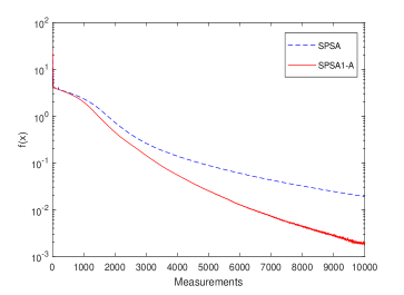
Figure 1: Minimizing the Rosenbrock function by Algorithms SPSA and SPSA1-A.

As shown in Figure 1, the logarithmic plot of the average number of function measurements, Algorithm SPSA1-A converges faster than SPSA. In particular, to output a solution of the same accuracy, say $f(x)<0.01$, Algorithm SPSA1-A requires less than half as many functional measurements as that of SPSA.

Problem $2$. (Beale function)

$$f(x)=[1.5-x_{1}(1-x_{2})]^{2}+[2.25-x_{1}(1-x_{2}^{2})]^{2}+[2.625-x_{1}(1-x_{2}^{3})]^{2}$$

We choose $x_{0}=(1,1)^{T}$ and $M=5000$. The parameters given in Table 2 are empirically the best for Algorithm SPSA.

Table 2: The parameters in Algorithms SPSA and SPSA1-A for Beale function.

	a	A	c	$\alpha$	$\gamma$
SPSA	1	30	0.1	1	0.16667
SPSA1-A	1	30	0.1	1	0.16667

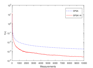
Figure 2: Minimizing the Beal function by Algorithms SPSA and SPSA1-A.

According to Figure 2, the logarithmic plot of the average number of function measurements, the iterative functional values by Algorithm SPSA1-A decreased much faster than that of SPSA in the first hundreds of functional measurements. After $M$ iterations, the accuracy of the solution outputted by Algorithm SPSA1-A is an order of magnitude higher than that of Algorithm SPSA.

Problem $3$. (Powell singular function)

$$f(x)=(x_{1}+10x_{2})^{2}+5(x_{3}-x_{4})^{2}+(x_{2}-2x_{3})^{4}+10(x_{1}-x_{4})^{4}$$

We choose $x_{0}=(3,-1,0,1)^{T}$ and $M=5000$. The parameters given in Table 3 are empirically the best for Algorithms SPSA and SPSA1-A, respectively.

Table 3: The parameters in Algorithms SPSA and SPSA1-A for Powell singular function.

	a	A	c	$\alpha$	$\gamma$
SPSA	0.08	1000	0.1	0.602	0.101
SPSA1-A	0.02	100	0.1	0.602	0.101

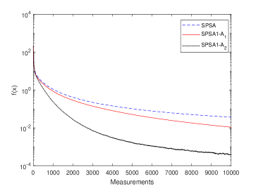
Figure 3: Minimizing the Powell singular function by Algorithms SPSA and SPSA1-A.

Algorithms SPSA1-A₁ and SPSA1-A₂ use the best parameters for Algorithms SPSA and SPSA1-A, respectively. As shown in the logarithm plot 3, both algorithms converge faster than Algorithm SPSA. Moreover, as expected, Algorithm SPSA1-A₂ highly outperforms SPSA1-A₁.

3.2 Test $II$

We numerically compare Algorithms SPSA, SPSA1-A and SPSA1 on the example presented for SPSA1 in spall1997one :

$$f(x)=x^{T}x+0.1\sum_{i=1}^{5}x_{i}^{3}+0.01\sum_{i=1}^{5}x_{i}^{4}.$$ (4)

All algorithms start from the same initial point $x_{0}=(3,-1,0,1)^{T}$ and stop when either the maximum iteration number $M=10^{5}$ is reached or the error $e_{k}=|f(x_{k})-f^{*}|$ is less than a threshold (see the last two columns of Tables 4 and 5). We test all algorithms with the same two kinds of parameters as that in spall1997one , see Column 2-6 in Tables 4 and 5.

Table 4: Numerical results for minimizing (4) based on the parameters of the first kind.

	a	A	c	$\alpha$	$\gamma$	$e_{k}\leq 10^{-2}$	$e_{k}\leq 10^{-3}$
SPSA	0.17	20	0.06	1	0.16667	206	7711
SPSA1	0.17	20	0.06	1	0.16667	3930	–
SPSA1-A	0.17	20	0.06	1	0.16667	80	784

Table 5: Numerical results for minimizing (4) based on the parameters of the second kind.

	a	A	c	$\alpha$	$\gamma$	$e_{k}\leq 10^{-2}$	$e_{k}\leq 10^{-3}$
SPSA	0.27	100	0.06	1	0.16667	349	3738
SPSA1	0.27	100	0.06	1	0.16667	2172	–
SPSA1-A	0.27	100	0.06	1	0.16667	144	711

We report the numbers of functional measurements of three algorithms until they terminate in the last two columns of Tables 4 and 5, where “–” stands for the situation that the maximum iteration number $M$ is reached. Clearly, Algorithm SPSA1-A performs much better than the other two algorithms. We also notice that Algorithm SPSA1 fails to find solution of high accuracy.

4 Conclusion

The simultaneous perturbation stochastic approximation (SPSA) algorithm is popular for minimizing a noised function. It measures two function values in each iteration. It makes sense that each iteration requires at least two functional measurements to guarantee the descent of the search direction. In this paper, we propose a new algorithm measuring two function values every two iterations, that is, only one measurement of function is taken per iteration in the average sense. We prove the strong convergence and asymptotic normality of the new algorithm. Numerical results demonstrate the effectiveness of our new algorithm comparing with Algorithm SPSA. Future works include more applications and further improvement of our new algorithm.

Appendix A Proof of Lemma 1.

Proof

We start from the observation

$$E[\hat{\xi}_{k}|\hat{x}_{k}]=E[E[\hat{\xi}_{k}|\hat{x}_{k},\hat{g}_{k}]|\hat{x}_{k}].$$

Notice that each component $\hat{\xi}_{ki}~{}(i=1,2,\cdots,n)$ of $\hat{\xi}_{k}$ obeys the symmetric Bernoulli distribution and satisfies ${\hat{\xi}_{k}}^{T}\hat{g}_{k}\geq 0$. Therefore, at least half of the components of $\hat{\xi}_{k}$ have the same sign as the components $\hat{g}_{ki}~{}(i=1,2,\cdots,n)$ of $\hat{g}_{k}$. If $n$ is even, $\hat{\xi}_{k}$ has $C_{n}^{n/2}+C_{n}^{n/2+1}+\cdots+C_{n}^{n}=2^{n-1}+C_{n}^{n/2}/2$ choices. So for any possible choice $\zeta_{j}$, we have

$$P(\hat{\xi}_{k}=\zeta_{j})=\frac{1}{2^{n-1}+C_{n}^{n/2}/2}.$$

If the signs of $\hat{\xi}_{ki}$ and $\hat{g}_{ki}$ $(\forall i\in\{1,2,\cdots,n\})$ are the same, then at least $n/2-1$ of the remaining $n-1$ elements of $\hat{\xi}_{k}$ share the same signs as that of $\hat{g}_{ki}$. In this case, $\hat{\xi}_{k}$ has $C_{n-1}^{(n-2)/2}+C_{n-1}^{n/2}+\cdots+C_{n-1}^{n-1}=2^{n-2}+C_{n-1}^{(n-2)/2}$ choices. Then we can write

$$\Sigma\zeta_{j} = \left\{2^{n-2}+C_{n-1}^{(n-2)/2}-\left[\left(2^{n-1}+C_{n}^{n/2}/2\right)-\left(2^{n-2}+C_{n-1}^{(n-2)/2}\right)\right]\right\}\text{sgn}\left(\hat{g}_{k}\right)$$

$$= \left(2C_{n-1}^{(n-2)/2}-C_{n}^{n/2}/2\right)\text{sgn}\left(\hat{g}_{k}\right)$$

$$= C_{n-1}^{n/2}\text{sgn}\left(\hat{g}_{k}\right).$$

If $n$ is odd, $\{\zeta_{j}\}$ has $C_{n}^{(n+1)/2}+C_{n}^{(n+1)/2+1}+\cdots+C_{n}^{n}=2^{n-1}$ choices, each with probability $P(\hat{\xi}_{k}=\zeta_{j})=1/2^{n-1}$. The sign of $\hat{\xi}_{ki}$ is either the same as or opposite to that of $\hat{g}_{ki}$. If their signs are the same, then at least $(n-1)/2$ of the remaining $n-1$ elements of $\hat{\xi}_{k}$ share the same signs as $\hat{g}_{ki}$. In this case, $\hat{\xi}_{k}$ has $C_{n-1}^{(n-1)/2}+C_{n-1}^{(n+1)/2}+\cdots+C_{n-1}^{n-1}=2^{n-2}+C_{n-1}^{(n-1)/2}/2$ choices. Then we can write

$$\Sigma\zeta_{j} = \left\{2^{n-2}+C_{n-1}^{(n-1)/2}/2-\left[2^{n-1}-\left(2^{n-2}+C_{n-1}^{(n-1)/2}/2\right)\right]\right\}\text{sgn}(\hat{g}_{k})$$

$$= C_{n-1}^{(n-1)/2}\text{sgn}\left(\hat{g}_{k}\right).$$

It then holds that

$$\Sigma\zeta_{j}P(\hat{\xi}_{k}=\zeta_{j})=\begin{cases}\frac{C_{n-1}^{n/2}}{2^{n-1}+C_{n}^{n/2}/2}\text{sgn}(\hat{g}_{k}),~{}&{\rm if}~{}n~{}{\rm is~{}even},\\ \frac{C_{n-1}^{(n-1)/2}}{2^{n-1}}\text{sgn}(\hat{g}_{k}),~{}&{\rm otherwise}.\\ \end{cases}$$

For $\rho$ defined in Step $1$ of Algorithm SPSA1-A, we have

$$E[E[\hat{\xi}_{k}|\hat{x}_{k},\hat{g}_{k}]|\hat{x}_{k}]=E[_{\hat{g}_{k}}\rho E[\text{sgn}(\hat{g}_{k})|\hat{x}_{k}]|\hat{x}_{k}]=\rho E[\text{sgn}(\hat{g}_{k})|\hat{x}_{k}].$$

Let $\rho_{k}=\rho/\|\hat{g}_{k}\|_{\infty}$. We can complete the proof

$$E[\hat{\xi}_{k}|\hat{x}_{k}]=E[\rho_{k}\hat{g}_{k}|\hat{x}_{k}].$$

Appendix B Proof of Lemma 2.

Proof

By a proof similar to that of Lemma 1, we have

$$E\left[\frac{\hat{\xi}_{k}}{1+\rho_{k}}\bigg{|}\hat{x}_{k}\right]=E\left[\frac{\rho_{k}}{1+\rho_{k}}\hat{g}_{k}\bigg{|}\hat{x}_{k}\right].$$

Then, we can obtain

$$b_{k}(\hat{x}_{k}) = {E[\hat{g}_{k}(\hat{x}_{k})-g(\hat{x}_{k})|\hat{x}_{k}]}.$$

In the sequel, the lemma can be proved similar to that in [13].

Appendix C Proof of Proposition 1.

Proof

According to [6], based on Lemma 2 and Assumption 1, we have

i)

$$\|b_{k}(\hat{x}_{k})\|<\infty~{}\forall~{}k~{}{\rm and}~{}b_{k}(\hat{x}_{k})\to 0,~{}a.s..$$

Next, we prove that

ii)

$$\lim\limits_{k\to\infty}P\left(\sup\limits_{m\geq k}\left\|\sum_{i=k}^{m}a_{i}e_{i}(\hat{x}_{i})\right\|\geq\eta\right)=0,~{}{\rm for~{}any}~{}\eta>0.$$

First, for any $l\in\{1,2,\cdots,n\}$, we have

$$Ee_{il}^{2} \leq Var\left(\frac{\hat{g}_{il}+\hat{\xi}_{il}}{1+\rho_{i}}\right)\leq E(\frac{\hat{g}_{il}+\hat{\xi}_{il}}{1+\rho_{i}})^{2}$$

$$= E\frac{\hat{g}_{il}^{2}}{(1+\rho_{i})^{2}}+2E\frac{\hat{g}_{il}\hat{\xi}_{il}}{(1+\rho_{i})^{2}}+E\frac{\hat{\xi}_{il}^{2}}{(1+\rho_{i})^{2}}.$$

Then we obtain

$$E\left(\hat{g}_{il}\hat{\xi}_{il}\right) \leq E\left(\left|\hat{g}_{il}\right|\cdot\left|\hat{\xi}_{il}\right|\right)$$

$$\leq E\left|\hat{g}_{il}\right|$$

$$\leq \frac{1}{2c_{i}}E\left[\left|\xi_{il}^{-1}\right|\cdot\left(\left|L(\hat{x}_{i}+c_{i}\xi_{i})\right|+\left|L(\hat{x}_{i}-c_{i}\xi_{i})\right|+\left|\varepsilon_{i}^{+}\right|+\left|\varepsilon_{i}^{-}\right|\right)\right]$$

$$\leq \left(\sqrt{\alpha_{0}}+\sqrt{\alpha_{1}}\right)c_{i}^{-1}.$$

It follows from [13] that

$$E\hat{g}_{il}^{2}\leq 2(\alpha_{1}+\alpha_{0})c_{i}^{-2}.$$

Since $\frac{1}{(1+\rho_{i})^{2}}=\frac{1}{(1+\rho/|g_{il}|)^{2}}\leq 1$ and $E\hat{\xi}_{il}^{2}=1$, we have

$$Ee_{il}^{2} \leq E\hat{g}_{il}^{2}+2E\hat{g}_{il}\hat{\xi}_{il}+E\hat{\xi}_{il}^{2}\leq 2(\alpha_{1}+\alpha_{0})c_{i}^{-2}+(\sqrt{\alpha_{0}}+\sqrt{\alpha_{1}})c_{i}^{-1}+1.$$

Therefore, it holds that

$$E\|e_{k}\|^{2}\leq p[2(\alpha_{1}+\alpha_{0})c_{k}^{-2}+(\sqrt{\alpha_{0}}+\sqrt{\alpha_{1}})c_{k}^{-1}+1].$$

Next, since $\{\sum_{i=k}^{m}a_{i}e_{i}\}_{m\geq k}$ is a martingale sequence, it follows from the inequality in [4, P. 315] (see also [6, P. 27]) that

$$P(\sup\limits_{m\geq k}\|\sum_{i=k}^{m}a_{i}e_{i}\|\geq\eta\|) \leq \eta^{-2}E\|\sum_{i=k}^{\infty}a_{i}e_{i}\|^{2}=\eta^{-2}\sum_{i=k}^{\infty}a_{i}^{2}E\|e_{i}\|^{2},$$ (5)

where the equality holds as $E\left[e_{i}^{T}e_{j}\right]=E\left[e_{i}^{T}E\left[e_{j}|\hat{x}_{j}\right]\right]=0,~{}\forall~{}i<j$.

Then, by (5) and Assumption 1, we complete the proof of ii).

Appendix D Proof of Proposition 2.

Proof

In order to complete the proof, we need to verify whether conditions (2.2.1), (2.2.2), and (2.2.3) in Fabian [5] are true. Here we assume that all assumptions on $\theta_{k}$ or $\mathscr{F}_{k}$ hold. According to the notation in [5], we can get

$$\hat{x}_{k+1}-x^{*}=(I-k^{-\alpha}\Gamma_{k})(\hat{x}_{k}-x^{*})+k^{-(\alpha+\beta)/2}\Phi_{k}V_{k}+k^{-\alpha-\beta/2}T_{k},$$

where $\Gamma_{k}=aH~{}(\overline{x}_{k})$, $V_{k}=k^{-\gamma}\left\{\frac{\hat{g}_{k}(\hat{x}_{k})+\hat{\xi}_{k}}{1+\rho_{k}}-E\left[\frac{\hat{g}_{k}(\hat{x}_{k})+\hat{\xi}_{k}}{1+\rho_{k}}\Big{|}\hat{x}_{k}\right]\right\}$, $\Phi_{k}=-aI$, and $T_{k}=-ak^{\beta/2}b_{k}(\hat{x}_{k})$. In fact, there is an open neighborhood of $\hat{x}_{k}$ (for $k$ sufficiently large) containing $x^{*}$ in which $H(\cdot)$ is continuous. Then

$$E\left[\frac{\hat{g}_{k}(\hat{x}_{k})+\hat{\xi}_{k}}{1+\rho_{k}}\bigg{|}\hat{x}_{k}\right] = H(\overline{x}_{k})(\hat{x}_{k}-x^{*})+b_{k}(x^{*}),$$

where $\Gamma_{k}=aH(\overline{x}_{k})$ lies in the line segment between $\hat{x}_{k}$ and $x^{*}$.

Based on the continuity of $H(\cdot)$ and a.s. convergence of $\hat{x}_{k}$, we have $\Gamma_{k}=aH(\overline{x}_{k})\rightarrow aH(x^{*})$ a.s..

Now we prove the convergence of $T_{k}$ for $3\gamma-\alpha/2\geq 0$. When $3\gamma-\alpha/2>0$, as $b_{k}(\hat{x}_{k})=O(k^{-2\gamma})$ a.s., we can write that $T_{k}\rightarrow 0$ a.s.. When $3\gamma-\alpha/2=0$, by the facts that $\hat{x}_{k}\rightarrow x^{*}$ a.s. and the uniformly boundedness of $L^{(3)}$ near $x^{*}$, we have

$$k^{2\gamma}b_{kl}(\hat{x}_{k})-\frac{1}{6}c^{2}L^{(3)}(x^{*})E(\xi_{k}\otimes\xi_{k}\otimes\xi_{k})\rightarrow 0~{}a.s..$$

Then ${\xi_{ki}}$ is symmetrically i.i.d. for each $k$, which means that the $l$-th element of $T_{k}$ satisfies that

$$T_{kl}\rightarrow-\frac{1}{6}ac^{2}{L_{lll}^{(3)}(x^{*})+\sum_{\begin{subarray}{c}i=1\\ i\neq l\end{subarray}}^{p}\left[L^{(3)}_{lii}(x^{*})+L_{ili}^{(3)}(x^{*})+L_{iil}^{(3)}(x^{*})\right]}~{}a.s..$$

Therefore, $T_{k}$ converges for $3\gamma-\alpha/2\geq 0$.

We can write

$$E\left[V_{k}V_{k}^{T}\big{|}\mathscr{F}_{k}\right] = k^{-2\gamma}\Bigg{\{}E\left[\frac{1}{(1+\rho_{k})^{2}}(\hat{g}_{k}+\hat{\xi}_{k})(\hat{g}_{k}+\hat{\xi}_{k})^{T}\bigg{|}\hat{x}_{k}\right]$$

$$~{}-E\left[\frac{1}{1+\rho_{k}}(\hat{g}_{k}+\hat{\xi}_{k})\bigg{|}\hat{x}_{k}\right]E\left[\frac{1}{1+\rho_{k}}(\hat{g}_{k}+\hat{\xi}_{k})^{T}\bigg{|}\hat{x}_{k}^{T}\right]\Bigg{\}},$$

where

$$k^{-2\gamma}E\bigg{[}\frac{1}{(1+\rho_{k})^{2}}(\hat{g}_{k}+\hat{\xi}_{k})(\hat{g}_{k}+\hat{\xi}_{k})^{T}\bigg{|}\hat{x}_{k}\bigg{]}$$

$$= k^{-2\gamma}E\left[\frac{1}{(1+\rho_{k})^{2}}(\hat{g}_{k}\hat{g}_{k}^{T}+\hat{g}_{k}\hat{\xi}_{k}^{T}+\hat{\xi}_{k}\hat{g}_{k}^{T}+\hat{\xi}_{k}\hat{\xi}_{k}^{T})\bigg{|}\hat{x}_{k}\right].$$

Define $\xi^{-1}_{k}:=(\xi^{-1}_{k1},\cdots,\xi^{-1}_{kp})^{T}$. Then we have

$$E\left[\frac{1}{(1+\rho_{k})^{2}}\hat{g}_{k}\hat{g}_{k}^{T}\bigg{|}\mathscr{F}_{k}\right] = E\left\{\frac{1}{(1+\rho_{k})^{2}}\xi_{k}^{-1}(\xi_{k}^{-1})^{T}\left[\frac{\varepsilon_{k}^{(+)}-\varepsilon_{k}^{(-)}}{2ck^{-\gamma}}\right]^{2}\bigg{|}\mathscr{F}_{k}\right\},$$ (6)

where

$$\frac{1}{(1+\rho_{k})^{2}}=\frac{1}{(1+\frac{\rho}{|\hat{g}_{kl}|})^{2}}=\frac{|\hat{g}_{kl}|^{2}}{(|g_{kl}|+\rho)^{2}}=\frac{[\frac{y^{(+)}-y^{(-)}}{2ck^{-\gamma}}]^{2}}{[\frac{y^{(+)}-y^{(-)}}{2ck^{-\gamma}}+\rho]^{2}}=\frac{[y^{(+)}-y^{(-)}]^{2}}{[y^{(+)}-y^{(-)}+2ck^{-\gamma}\rho]^{2}},$$

and the last equation $\rightarrow 1$ with $k\rightarrow\infty$. Therefore, (6) is same as the third term in (3.5) in [13]. As the element of $\hat{g}_{k}\hat{\xi}_{k}^{T}+\hat{\xi}_{k}\hat{g}_{k}^{T}+\hat{\xi}_{k}\hat{\xi}_{k}^{T}$ is bounded, we have

$$k^{-2\gamma}E\bigg{[}\frac{1}{(1+\rho_{k})^{2}}\left(\hat{g}_{k}\hat{\xi}_{k}^{T}+\hat{\xi}_{k}\hat{g}_{k}^{T}+\hat{\xi}_{k}\hat{\xi}_{k}^{T}\right)\bigg{|}\hat{x}_{k}\bigg{]}\rightarrow 0,$$

and

$$E\left[\frac{1}{1+\rho_{k}}(\hat{g}_{k}+\hat{\xi}_{k})\bigg{|}\hat{x}_{k}\right]E\left[\frac{1}{1+\rho_{k}}(\hat{g}_{k}+\hat{\xi}_{k})^{T}\bigg{|}\hat{x}_{k}^{T}\right]=E\left(\hat{g}_{k}\big{|}\hat{x}_{k}\right)E\left(\hat{g}_{k}^{T}\big{|}\hat{x}_{k}^{T}\right).$$

According to [13], we obtain

$$E\left(V_{k}V_{k}^{T}\big{|}\mathscr{F}_{k}\right)\rightarrow\frac{1}{4}c^{-2}\sigma^{2}I~{}~{}~{}~{}a.s..$$

Thus we have obtained the conditions (2.2.1) and (2.2.2) of [5]. Next we prove condition (2.2.3), i.e.,

$$\lim\limits_{k\rightarrow\infty}E\big{(}\mathscr{I}_{\{\left\|V_{k}\right\|^{2}\geq rk^{\alpha}\}}\left\|V_{k}\right\|^{2}\big{)}=0~{}~{}~{}\forall r>0.$$

By Holder’s inequality and $0<\delta^{\prime}<\delta/2$, the upper bound of the above limit can be obtained as

$$\lim\limits_{k\rightarrow\infty}\sup P(\left\|V_{k}\right\|^{2}\geq rk^{\alpha})^{\delta^{\prime}/(1+\delta^{\prime})}(E\left\|V_{k}\right\|^{2(1+\delta^{\prime})})^{1/(1+\delta^{\prime})}$$

$$\leq \lim\limits_{k\rightarrow\infty}\sup\left(\frac{E\left\|V_{k}\right\|^{2}}{rk^{\alpha}}\right)^{\delta^{\prime}/(1+\delta^{\prime})}(E\left\|V_{k}\right\|^{2(1+\delta^{\prime})})^{1/(1+\delta^{\prime})}.$$

Notice that

$$\left\|V_{k}\right\|^{2(1+\delta^{\prime})}\leq 2^{2(1+\delta^{\prime})}k^{-2(1+\delta^{\prime})\gamma}\bigg{[}\left\|\frac{\hat{g}_{k}+\hat{\xi}_{k}}{1+\rho_{k}}\right\|^{2}+\left\|b_{k}\right\|^{2}+\left\|g_{k}\right\|^{2}\bigg{]}.$$

Then the proof is completed following from the proof of [13, Proposition 1].

References

- [1] M. U. Altaf, A. W. Heemink, M. Verlaan, I. Hoteit, Simultaneous perturbation stochastic approximation for tidal models, Ocean dynamics, 61(8) (2001) 1093-1105.
- [2] A. T. Abdulsadda, K. Iqbal, An improved algorithm for system identification using fuzzy rules for training neural networks, International journal of automation and computing, 8(3) (2001) 333-339.
- [3] V. Bartkutė, L. Sakalauskas, Simultaneous perturbation stochastic approximation of nonsmooth functions, European journal of operational research, 181(3) (2007) 397-409.
- [4] J. L. Doob, Stochastic processes, John wiley and sons, 1953.
- [5] V. Fabian, On asymptotic normality in stochastic approximation, The annals of mathematical statistics, 39(4) (1968) 1327-1332.
- [6] H. J. Kushner, D. S. Clark, Stochastic approximation methods for constrained and unconstrained systems, Springer publisher, 1978.
- [7] J. Kiefer, J. Wolfowitz, Stochastic estimation of the maximum of a regression function, The annals of mathematical statistics, 23(3) (1952) 462-466.
- [8] J. J. Moré, B. S. Garbow, K. E. Hillstrom, Testing unconstrained optimization software, ACM transactions on mathematical software, 7(1) (1981) 17-41.
- [9] H. Robbins, S. Monro, A stochastic approximation method, The annals of mathematical statistics, 22(3) (1951) 400-407.
- [10] J. C. Spall, A one-measurement form of simultaneous perturbation stochastic approximation, Automatica, 33(1) (1997) 109-112.
- [11] J. C. Spall, Accelerated second-order stochastic optimization using only function measurements, Proceedings of the 36th IEEE conference on decision and control, 2 (1997) 1417–1424.
- [12] J. C. Spall, Implementation of the simultaneous perturbation algorithm for stochastic optimization, IEEE transactions on aerospace and electronic systems, 34(3) (1998) 817-823.
- [13] J. C. Spall, Multivariate stochastic approximation using a simultaneous perturbation gradient approximation, IEEE transactions on automatic control, 37(3) (1992) 332-341.
- [14] J. C. Spall, Stochastic version of second-order (Newton-Raphson) optimization using only function measurements, Proceedings of the 1995 winter simulation conference, (1995) 347-352.
- [15] P. Sadegh, J. C. Spall, Optimal random perturbations for stochastic approximation using a simultaneous perturbation gradient approximation, IEEE transactions on automatic control, 43(10) (1998) 1480-1484.
- [16] Z. Xu, Y. H. Dai, A stochastic approximation frame algorithm with adaptive directions, Numerical mathematics: theory, methods and applications, 1(4) (2008) 460–474.
- [17] X. Zhu, J. C. Spall, A modified second-order SPSA optimization algorithm for finite samples, International journal of adaptive control and signal processing, 16(5) (2002) 397-409.