The Infrared Database of Extragalactic Observables from Spitzer. –
II. The Database & The Diagnostic Power of Crystalline Silicate Features in Galaxy Spectra

Abstract

We present the Infrared Database of Extragalactic Observables from Spitzer (IDEOS), a homogeneous, publicly available, database of 77 fitted mid-infrared observables in the 5.4–36 $\mu$m range, comprising measurements for 3335 galaxies observed in the low-resolution staring mode of the Infrared Spectrometer onboard the Spitzer Space Telescope. Among the included observables are PAH fluxes and their equivalent widths, the strength of the 9.8 $\mu$m silicate feature, emission line fluxes, solid-state features, rest frame continuum fluxes, synthetic photometry, and a mid-infrared spectral classification. The IDEOS spectra were selected from the Cornell Atlas of Spitzer-IRS Sources. To our surprise we have detected at a $>$95% confidence level crystalline silicates in the spectra of 786 IDEOS galaxies. The detections range from single band detections to detections of all fitted crystalline bands (16, 19, 23, 28 and 33 $\mu$m). We find the strength of the crystalline silicate bands to correlate with the amorphous silicate strength, and the change from an emission to an absorption feature to occur at higher obscuration as the wavelength of the crystalline silicate band is longer. These observed characteristics are consistent with an origin for the amorphous and crystalline silicate features in a centrally heated dust geometry, either an edge-on disk or a cocoon. We find the 23 and 33 $\mu$m crystalline silicate bands to be well-suited to classify the obscuration level of galactic nuclei, even in the presence of strong circumnuclear star formation. Based on our detection statistics, we conclude that crystalline silicates are a common component of the interstellar medium of galactic nuclei.

1 Introduction

The successful mission of the Spitzer Space Telescope (2003-2020; Werner et al., 2004) has bestowed us with a rich scientific legacy comprising many thousands of publications. In many cases the data that these papers are based on were extracted by researchers with extensive experience in Spitzer data processing.

The individual calibrated frames obtained by the Spitzer instruments, or basic calibrated data (BCD) in Spitzer speak, are available from the Spitzer Heritage Archive (SHA). This is also where the combined frames, extracted spectra, and celestial maps, the so-called post-BCD products, can be searched and downloaded from.

To fill the gap between the bulk-processed products offered by the SHA and the level of processing that an instrument specialist can attain, the members of the Infrared Spectrograph (IRS; Houck et al., 2004) team at Cornell University created CASSIS, the Cornell Atlas of Spitzer/Infrared Spectrograph Sources(Lebouteiller et al., 2011). For each IRS staring-mode observation CASSIS offers the choice of several background subtraction options and several spectral extraction methods, all of which can be visually compared to select and download the best spectrum for the source at hand.

In 2012 we took the next logical step and started working on the Infrared Database of Extragalactic Observables from Spitzer (IDEOS). IDEOS builds on the publication-quality IRS spectra in the CASSIS repository by providing a homogeneous set of measurements of spectral features and continuum flux densities resulting from fitting and decomposing the IRS low-resolution spectra (R=60–120) of a subset of 3335 extragalactic sources. The selection of the IDEOS spectra and the preparation for their analysis are described in Hernán-Caballero et al. (2016) (Paper i; see also Sect. 2). In the present paper (Paper ii) we describe our fitting methods and present our observables. Technical details on the IRS modules and their characteristics can be found in Houck et al. (2004).

A large sample of homogeneously measured observables, like IDEOS, allows for the search for subtle trends that would remain elusive in smaller or heterogeneously measured data sets. In Sect. 9 we present an analysis of a number of weak absorption and emission features resulting from the presence of crystalline silicates in the interstellar medium (ISM) of IDEOS galaxies.

Observations with the Infrared Space Observatory (ISO) in the 1990s have shown crystalline silicates to be a common component of interstellar dust in circumstellar environments (Molster & Kemper, 2005, and references there in). In contrast, ISO observations of the diffuse ISM, as probed by the line of sight to Sgr A^∗, have set a clear upper limit of 1% to the crystallinity of the diffuse ISM in our galaxy (Kemper et al., 2004, 2005). The presence of crystalline silicates in extragalactic environments only became known in 2006 through their detection in the strongly silicate-absorbed Spitzer-IRS spectra of twelve deeply enshrouded Ultraluminous Infrared Galaxies (ULIRGs; Spoon et al., 2006).

In recent years, X-ray Si K-band absorption edge studies have revealed the presence of a fraction of crystalline silicates in the ISM of about 0.1, well exceeding the infrared upper limits (Zeegers et al., 2019; Rogantini et al., 2019). The difference has been attributed to the presence of polycrystalline silicate grains in the ISM, which register as crystalline structures using X-ray techniques (sensitive to short range lattice order) and as amorphous in infrared observations (probing long range lattice disorder). Further studies will be needed to reconcile these findings.

Because crystallization of silicates is inhibited by high energy barriers, the presence of crystalline silicate features in a mid-infrared spectrum is indicative of processing of grains in the circumstellar and/or interstellar medium. While in Galactic environments this points to origins in both pre-main-sequence and post-main-sequence stars, in active galaxies radiation from the accretion disk around supermassive black holes may be another source of energetic processing (Spoon et al., 2006), while shocks may play a role in interacting galaxies.

The complete absence of absorption features of crystalline silicates in mid-infrared spectra of the Galactic ISM (Kemper et al., 2004) implies a rapid transformation of newly formed crystalline silicates into amorphous silicates in the interstellar medium ($\leq$10⁸ yr; Kemper et al., 2004). This amorphization may be achieved through sputtering of the dust in strong shock waves resulting from supernova explosions (Jones et al., 1994, 1996), but would, however, likely affect amorphous and crystalline silicates equally and thus leave their proportions unchanged. Cosmic rays, produced in the same supernova events, are thought to be more effective in reducing the crystalline silicate fraction, and may act on timescales of $\sim$10⁷ years (Bringa et al., 2007).

For their sample of twelve ULIRGs Spoon et al. (2006) concluded that amorphization due to cosmic rays may lag in vigorous starburst environments, leaving enough freshly forged crystalline silicates in the ISM to be detectable in their galaxy spectra. Our present far larger study puts the need for these special conditions in doubt.

Our paper is organized as follows. Section 2 provides a brief description of how we processed spectra selected from the CASSIS repository for ingestion in the IDEOS database. Section 3 describes in detail our method and assumption for fitting the IDEOS SEDs to obtain observables. Section 4 details how we deployed the spectral decomposition tools PAHFIT and QUESTFIT to obtain alternate sets of observables for our sample. Sections 5 and 6 describe how we compute rest frame continuum fluxes and synthetic photometry, respectively. Section 7 explains our method for deriving silicate strengths. Section 8 discusses what can be learned from mid-infrared diagnostic plots containing thousands of IDEOS sources. Section 9 analyses the crystalline silicate features that we detected. Section 10 presents the IDEOS web portal. Section 11 contains the discussion and our conclusions.

2 The IDEOS spectra

Table 1: IDEOS sample statistics

CASSIS spectra in extragalactic or calibration programs (ECPs)	5015
CASSIS spectra in ECPs: no detection	1263
CASSIS spectra in ECPs: detection in single nod	50
CASSIS spectra in ECPs: Local Group galaxy or non-nuclear pointing	200
IDEOS galaxy spectra	3558
IDEOS galaxy spectra: appended with segments from other observations	80
IDEOS galaxies	3335
IDEOS galaxies with multiple observations of 1–4 segment(s)	110
IDEOS galaxies with averaged spectra from multiple observations	25
IDEOS BLAZARs with low and high-state spectra: 3C 279 and 3C 454.3	2
IDEOS galaxies at redshifts $\leq$0.1	1463
IDEOS galaxies at redshifts 0.1–0.2	456
IDEOS galaxies at redshifts 0.2–0.4	334
IDEOS galaxies at redshifts 0.4–0.6	166
IDEOS galaxies at redshifts 0.6–0.8	167
IDEOS galaxies at redshifts 0.8–1.0	197
IDEOS galaxies at redshifts 1.0–2.0	350
IDEOS galaxies at redshifts $\geq$2	204
IDEOS galaxies with a silicate strength (Ssil) measurement	2846
IDEOS galaxies with Ssil$\geq$-1	2527
IDEOS galaxies with Ssil$<$-1	319

The 3558 spectra that are part of IDEOS have been selected from a parent sample of 5015 spectra from CASSIS that met our initial selection requirement of belonging to an extragalactic Spitzer-IRS observing, science-demonstration, or calibration program. Of the 5015 spectra, 1263 spectra did not result in a source detection, and another 50/5015 were detected in only one nod spectrum or only in a bonus order. Of the remaining spectra, some 200 were discarded for mispointing, for a non-nuclear pointing (e.g. an observation of a supernova), for bad background-subtraction (in a crowded field), or for requiring large and uncertain aperture corrections due to membership of the Local Group of galaxies. As is true for all CASSIS spectra, the IDEOS sample consists purely of spectra obtained in staring mode (as opposed to mapping mode).

In order to be able to measure observables from the IDEOS spectra, each extracted spectrum is first identified in the NASA Extragalactic Database (NED), is assigned a redshift, and has its spectral segments (orders) scaled and stitched. In addition, for 80 incomplete spectra we were able to find and append additional spectral segments from other observation of the same target. A detailed description of these steps is provided in Paper i.

We spent great care to define meaningful fitting uncertainties for the IDEOS observables. It is important to realize, though, that these uncertainties do not include uncertainties associated with the flux calibration, slit losses, or stitching of the spectral segments. Uncertainties in the latter are compounded from segment LL1 to LL2 to SL1 to SL2, where we assume the scaling factor of the LL1 segment to be unity (see Paper i). The segment-to-segment scaling uncertainties are generally small ($<$5%) but can be 10%–20% for the LL2 to SL1 scaling for low S/N spectra of semi-extended sources, as it is hard to determine whether the flux in the small order overlap is affected by excessive noise and spurious features or not. The IDEOS portal (see Sect. 10) provides information about unusual stitching uncertainties as part of the stitching metadata for each spectrum.

Among the 3558 IDEOS spectra we found 110 targets that had multiple observations (380) of some or all spectral segments (SL2/SL1/LL2/LL1). For 25 of these targets it was beneficial to the S/N of the spectrum to average these observations. Among them are Arp 220, IRAS 08572+3915NW, 3C 273, IRAS 07598+6508, and Mrk 231. For the remaining targets we identified the spectrum with the best S/N and use that spectrum in scatter plots as well as in statistical computations in this paper. The total number of unique IDEOS targets is 3335.

Note that the IDEOS portal (Sect. 10) provides observables for all 3558 spectra, not just for the 3335 best versions.

3 Spectral fitting

We have used the Levenberg-Marquardt least-squares fitting software package MPFIT (Markwardt, 2009) and empirical spectral templates to measure fluxes of emission features, optical depths of absorption features, and flux densities of the continuum in six rest frame ranges of the mid-infrared spectrum. The ranges are modelled independently from one another, without any prior assumptions on the underlying continuum other than it being a polynomial of a pre-defined order. The latter choice was made to ensure the best possible fit to the individual features. We will refer to this approach as ’chunk fitting’, and the code that implements it as ’CHUNKFIT’.

The features fitted in the six ranges comprise various PAH emission bands, fine-structure lines, pure rotational molecular hydrogen lines, crystalline silicate features, and absorption bands of water ice and aliphatic hydrocarbons. Not fitted are the 7.7 and 8.6 $\mu$m PAH features, as the proximity of the 9.8 $\mu$m silicate band makes it hard to determine a local continuum. We also do not fit the PAH plateau emission in the 5–18 $\mu$m range. This is a consequence of our choice to define the local continuum in this range using the method of Hony et al. (2001) and Vermeij et al. (2002), which lumps in the PAH plateau emission with the continuum emission. As an alternative, in Sect. 4 we will use the method of Smith et al. (2007), based on the PAH model of Boulanger et al. (1998), which does separate out the PAH plateau emission from the continuum emission. A comparison of both approaches is offered by Galliano et al. (2008b).

We further refrain from using silicate opacity profiles to model the local continua in the CHUNKFIT ranges affected by the amorphous silicate features centered at 9.8 $\mu$m and 18 $\mu$m, as these profiles may not be applicable to all galaxy-integrated spectra and could result in bad fits to the local continua and thus to the weak emission and absorption features we are trying to fit. We instead model the local continuum using polynomials, irrespective of whether the continuum is shaped by a silicate feature, or not. In Sect. 7 we describe the method we use to infer the strength of the 9.8 $\mu$m amorphous silicate feature.

In CHUNKFIT emission lines are modeled with gaussian profiles. An adequate choice given the gaussian shape of the IRS instrumental profile. Table 2 lists the spectral resolving powers from which our line widths derive.

Table 2: Spitzer-IRS characteristics

Module	Wavelength Range	Resolving power	Slit width
	[$\mu$m]		[′′]
SL2	5.13 – 7.60	85–125	3.6
SL1	7.46 – 14.29	61–120	3.7
LL2	13.90 – 21.27	82–125	10.5
LL1	19.91 – 39.90	58–112	10.7

Fitting features in spectra with a range of signal-to-noise (S/N) has proven challenging. In high S/N spectra, weak features can only be fitted well if the order of the polynomial continuum is high enough to provide an accurate fit to the local continuum. In contrast, in spectra of low S/N the same high degree of freedom for the continuum spectral shape will result in wavy continua as MPFIT will attempt to fit some of the noise spurious features. This challenge is especially large in spectral ranges that include the 9.7 and 18.5 $\mu$m silicate features, where the continuum spectral structure can show strong curvature. We therefore devised S/N criteria for when to limit the polynomial order to mitigate waviness. These criteria are different for different spectral ranges and depend on S/N as well as on the strength of specific spectral features in these ranges.

To minimize the number of false detections of emission lines, it would seem prudent to fix the line center to the rest wavelength and to fix the width of the line profile to the instrumental resolution at the observed wavelength. In practice, however, MPFIT fits a higher fraction of the lines present when the line center is allowed to shift by $\pm$600 km/s, and the line width is allowed to vary by $\pm$10%. Note that at the low spectral resolving power of the IRS low-resolution modules line asymmetries and line broadening associated with ionized gas outflows in AGN (Dasyra et al., 2008) and ULIRGs (Spoon et al., 2009a) cannot be resolved. It therefore is safe to assume that all emission lines have gaussian line profiles. For PAH features we use a different approach to limit false detections. Since a strong detection of an intrinsically weak PAH band likely indicates that a noise feature was fitted, we constrain the allowed ratio of a faint to a strong PAH feature to an empirically determined range measured from a sample of high S/N PAH spectra.

Table 3: Parameters in CHUNKFIT ranges

Range	Fit parameters	Degrees of freedom
5.39–7.25 $\mu$m	$\leq$24	20–61
8.7–10.3 $\mu$m	$\leq$19	13–47
10.0–12.58 $\mu$m	$\leq$21	14–48
9.8–13.5 $\mu$m	$\leq$31	24–66
13.0–15.4 $\mu$m	$\leq$14	11–34
14.4–16.2 $\mu$m	$\leq$8	6–25
14.5–21.0 $\mu$m	$\leq$28	33–72
19.0–36.5 $\mu$m	$\leq$30	47–113

MPFIT does not compute upper limits for spectral features it deems unnecessary to use in a fit, nor does it check whether features that it does fit constitute true detections. Upon completion of a CHUNKFIT model we therefore impose upper limits on a spectral feature if the height of that feature is less than three times the RMS noise divided by the square root of the number of spectral data points within the full width of the feature at 70% of the peak flux (FW70). The latter factor lowers the threshold for PAH features to be deemed detected, as the FW70 of a PAH feature is higher than for an emission line. A complication in this effort arises from the fact that for most CASSIS spectra the formal RMS uncertainty of the spectra is overestimated by up to a factor 3 when compared to the dispersion of flux values between nearby pixels in continuum regions of the spectrum. We therefore base the criterion for when and how to impose upper limits on local rather than on formal noise measurements.

In the subsections below we describe the CHUNKFIT models for six rest frame ranges. The maximum number of free parameters and the degrees of freedom in the models are listed in Table 3. None of the features fitted are extinction corrected in the process.

3.1 Features in the 5.39–7.25 $\mu$m range

For the 5.39–7.25 $\mu$m spectral range our CHUNKFIT model comprises the following spectral components:

• A 6 $\mu$m water ice absorption feature, derived from the spectrum of NGC 4418 (see Appendix A for details; Spoon et al., 2001).

• A 6.85 $\mu$m aliphatic C-H deformation mode absorption feature, derived from the spectrum of NGC 4418 (see Appendix A for details; Spoon et al., 2001)

• The absorption-corrected 5.39–7.25 $\mu$m continuum C_cor($\lambda$), represented by a third order polynomial function, and related to the local absorbed continuum C_abs($\lambda$) by C_abs($\lambda$)=C_cor($\lambda$) e${}^{-\tau_{\rm ice}(\lambda)-\tau_{\rm 6.85}(\lambda)}$. where $\tau_{\rm ice}$ is the optical depth in the 6.0 $\mu$m water ice feature and $\tau_{\rm 6.85}$ is the optical depth in the aliphatic C-H deformation mode absorption feature.

• PAH emission bands at 5.68, 6.04, and 6.22 $\mu$m (PAH57, PAH60 and PAH62, hereafter). While the former bands are best represented by Gaussian profiles, the asymmetric profile of the 6.2 $\mu$m feature (e.g. Hony et al., 2000) is best fitted by the asymmetric shape of a Pearson type-IV distribution (see Appendix B).

• Emission lines of H₂ 0–0 S(7) at 5.51 $\mu$m; of H₂ 0–0 S(5) at 6.91 $\mu$m; and of [Ar ii] at 6.99 $\mu$m, all modeled by Gaussian profiles.

In our model, only the continuum component is subject to attenuation by water ice (6 $\mu$m) and/or aliphatic hydrocarbons (6.85 $\mu$m). This assumption is in line with spectral decomposition models for buried galactic nuclei (e.g. Veilleux et al., 2009) in which the emission lines and PAH features are assumed to have a circum-nuclear origin, and are hence unaffected by water ice and aliphatic hydrocarbon absorption occuring within the nucleus. As a consequence, the equivalent width (EQW) of the PAH62 feature is computed using the absorption-corrected rather than the absorbed 6.22 $\mu$m continuum. An example fit for a strongly ice and hydrocarbon absorbed spectrum is shown in Fig. 1. Note that CHUNKFIT’s measured optical depths will be lower limits to the true optical depths in sources with strong circumnuclear PAH emission. The emission of overlapping wings of the PAH features will fill in the absorption features in these sources.

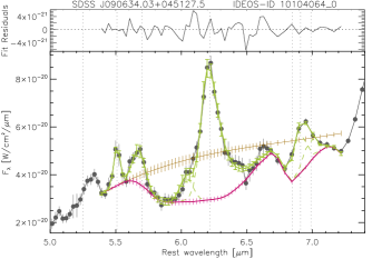
Figure 1: Example of a fit to the 5.39–7.25 $\mu$m spectrum of an IDEOS source. The observed spectrum is shown as black connected dots, the fit to the data in green. Individual emission features are shown as green dashed curves on top of the local absorbed continuum (pink). The absorption-corrected continuum inferred from the fit is shown in brown. Vertical dotted lines denote commonly detected features: 5.27$\mu$m PAH, 5.51$\mu$m H₂ S(7), 5.70$\mu$m PAH, 6.22$\mu$m PAH, 6.85 & 7.25$\mu$m CH₃/CH₂ deformation modes, 6.91$\mu$m H₂ S(5), 6.99$\mu$m [Ar ii].

The number of free parameters compared to the number of spectral data points in the 5.39–7.25 $\mu$m range is large. To avoid reducing the degrees of freedom of our model to below zero, the following lines are not included. [Mg vii] at 5.50 $\mu$m and [Mg v] at 5.61 $\mu$m. These magnesium lines are not commonly detected as it takes 109 eV and 186 eV, respectively, to create Mg⁴⁺ and Mg⁶⁺. This means that these lines only arise in AGN and will only be discernable in high S/N spectra. On top of that [Mg vii] is severely blended with H₂ 0–0 S(7), which is much more commonly detected in our sample. Adding [Mg v] at 5.61 $\mu$m to our model would overcrowd the 5.4–6.0 $\mu$m fit range, effectively creating a three line blend. We further do not include the 6.11 $\mu$m H₂ 0–0 S(6) line, which is generally faint.

To avoid false detections of PAH57 and PAH60 in low S/N spectra, we restrict the strength of the PAH57 and PAH60 bands to an empirically derived limit of 15% of the much stronger PAH62 band. To ensure realistic continuum fits also in low S/N spectra, we reduce the order of the polynomial continuum function from three to one in spectra that exhibit a S/N$<$6 at 6.6 $\mu$m in the continuum.

A (moderately) deep depression between the PAH57 and PAH62 features is a tell-tale signature of 6 $\mu$m water ice absorption (e.g. Fig. 1; Spoon et al., 2001). Careful inspection of individual fits to sources with weak to moderate depressions between the PAH57 and PAH62 features revealed that CHUNKFIT in most cases refrained from fitting a water ice feature, and instead prefers an unphysical concave continuum. In these cases (2/3 of the sources that we have identified ice in by visual inspection) we intervene by not allowing CHUNKFIT to drop the water ice feature from consideration. In 10% of these cases this is not enough, requiring another incentive to fit water ice: lowering the polynomial order of the ice-corrected continuum C_cor from three to one. Note that for sources for which fitting a water ice feature is a subjective choice, as it is for weak absorptions, this is reflected in the uncertainty in the fitted absorbed continuum C_abs, ice-corrected continuum C_cor, PAH62 flux, and PAH62 equivalent width, which are all elevated. In the IDEOS portal (see Sect. 10) we show examples of the effect of these interventions on the measured PAH62 quantities.

Finally, a point of caution. Measurements for the partially blended H₂ 0–0 S(5) and [Ar ii] lines in sources with a strong aliphatic hydrocarbon absorption band rely on the accuracy of the adopted absorption profile of the aliphatic hydrocarbon absorption band (see Appendix A). This is only partially reflected in the uncertainty of the fitted line fluxes.

3.2 Features in the 8.7–10.3 $\mu$m range

There are two emission lines in the 8.7–10.3 $\mu$m range which cannot be observed in the IRS high-resolution modules in low redshift sources, [Ar iii] at 8.99 $\mu$m and H₂ 0–0 S(3) at 9.66 $\mu$m. For these we created a separate CHUNKFIT model, which comprises the following spectral components:

• The 8.7–10.3 $\mu$m continuum, represented by a fifth order polynomial function.

• Emission lines of [Ar iii] at 8.99 $\mu$m and H₂ 0–0 S(3) at 9.66 $\mu$m, represented by Gaussian profiles.

An example of a model fit for the 8.7–10.3 $\mu$m range is shown in Fig. 2.

To ensure realistic continuum fits also in low S/N spectra, we lower the order of the polynomial continuum function from five to two in spectra that exhibit a continuum S/N$<$7 in the 9 $\mu$m range.

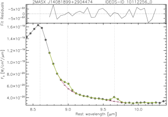
Figure 2: Example of a fit to the 8.7–10.3 $\mu$m spectrum of an IDEOS source. The observed spectrum is shown in black, the fit to the data in green, and the fitted local continuum in pink. Vertical dotted lines denote commonly detected features: 8.6$\mu$m PAH, 8.99$\mu$m [Ar iii], 9.66$\mu$m H₂ S(3).

3.3 Features in the 9.8–13.5 $\mu$m range

For fitting the 9.8–13.5 $\mu$m range we use a two-stage approach. First we model the features in the 10.0–12.58 $\mu$m spectral range and then repeat the fitting for an expanded range of 9.8–13.5 $\mu$m, using results from the 10.0–12.58 $\mu$m model as constraints.

Our CHUNKFIT model for the 10.0–12.58 $\mu$m range comprises the following spectral components:

• The 10.0–12.58 $\mu$m continuum, represented by a third order polynomial function. This continuum may exhibit strong curvature in spectra that are strongly affected by silicate emission or absorption.

• PAH emission bands at 10.64, 11.04, 11.25 and 12.00 $\mu$m (PAH107, PAH111, PAH112 and PAH120 hereafter). Like the PAH62 feature, the PAH112 feature is represented by an asymmetric Pearson type-IV distribution profile (see Appendix B, to account for the asymmetric nature of the feature (e.g. Hony et al., 2000). The other three bands are fitted by Gaussian profiles.

• Emission lines of [S iv] at 10.51 $\mu$m and H₂ 0–0 S(2) at 12.28 $\mu$m, represented by Gaussian profiles.

To ensure realistic continuum fits also in low S/N spectra, we lower the order of the polynomial continuum function from three to one in spectra that exhibit a continuum S/N$<$7 in the 10.65–11.95 $\mu$m range. If, however, the spectrum is PAH-dominated (i.e. the equivalent width of the PAH112 feature is more than 0.6 $\mu$m), the continuum S/N has to drop below 3 before a first order polynomial continuum is invoked, because PAH-dominated spectra have intrinsically weaker continua in the 10.65–11.95 $\mu$m range than continuum-dominated spectra. An example model fit is shown in Fig. 3.

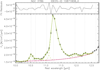
Figure 3: Example of a ’stage-1’ fit to the 10.0–12.58 $\mu$m spectrum of an IDEOS source. The observed spectrum is shown in black, and the fit to the data in green. Individual emission features are shown as green dashed curves on top of the local continuum (pink). Vertical dotted lines denote commonly detected features: 10.51$\mu$m [S iv], 10.64, 11.04, 11.29, 11.98$\mu$m PAH, and 12.28$\mu$m H₂ S(2).

In the second stage we expand the wavelength coverage of our CHUNKFIT model to 9.8–13.5 $\mu$m to include the PAH feature at 12.65 $\mu$m (PAH127) and the [Ne ii] line at 12.81 $\mu$m in our model. The [Ne ii] line is represented by a Gaussian profile and the asymmetric PAH127 feature by a Pearson IV profile (Appendix B).

Extension of the wavelength coverage requires the continuum to be fitted with a higher order polynomial function than for the 10.0–12.58 $\mu$m range, requiring a fourth to sixth order polynomial function, depending on the depth of the silicate feature. Only at low S/N we restrict the polynomial order to second order to avoid spectral artefacts and noise features to be fitted as if they were true continuum.

To ensure consistency between the two fitting stages, features that were deemed non-detected in the first stage are excluded in the second stage. An example model fit is shown in Fig. 4.

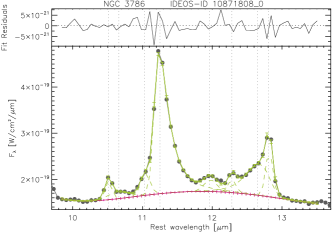
Figure 4: Example of a ’stage-2’ fit to the 9.8–13.5 $\mu$m spectrum of an IDEOS source. The observed spectrum is shown in black, and the fit to the data in green. Individual emission features are shown as green dashed curves on top of the local continuum (pink). Vertical dotted lines denote commonly detected features: 10.51$\mu$m [S iv], 10.64, 11.04, 11.29, 11.98, 12.63$\mu$m PAH, 12.28$\mu$m H₂ S(2), and 12.81$\mu$m [Ne ii].

As can be clearly seen when comparing Figs. 3 and 4, the stage-2 continuum more closely ressembles the spline continuum as intended by Hony et al. (2001) and Vermeij et al. (2002) than the stage-1 continuum does. Therefore, barring a lack in spectral coverage beyond 12.58 $\mu$m, the IDEOS observables for the features in this wavelength range are obtained from the stage-2 CHUNKFIT model. The only exception is the H₂ 0–0 S(2) line at 12.28 $\mu$m, which sometimes is fitted more accurately in the 10.0–12.58 $\mu$m (first stage) model, where the blue wing of the PAH127 feature is treated as continuum.

To avoid mistaking noise features and artefacts for faint PAH emission bands, we bootstrap the strength of the PAH107, PAH111, and PAH120 bands in our models to the much stronger PAH112 band. The maximum allowed relative strengths are listed in column three of Table 4. Only for the PAH127 band, which can be stronger than the PAH112 band (Hony et al., 2001), the ratio exceeds unity. For the same reason we also restrict the widths of the PAH bands. The allowed FWHM ranges are shown in column four of Table 4.

Finally, our 9.8–13.5 and 10.0–12.58 $\mu$m models do not include the hydrogen Hu-$\alpha$ recombination line at 12.37 $\mu$m as it is too weak to be detected at the resolving power of IRS SL and LL.

Table 4: Constraints on 9.8–13.5 $\mu$m PAH features

Feature	$\lambda_{0}$	F(PAH)/F(PAH112)	FWHM range
	($\mu$m)		($\mu$m)
PAH107	10.64	$\leq$0.10	0.141 – 0.352
PAH111	11.04	$\leq$0.13	0.118 – 0.165
PAH112	11.29	1.0	0.241 – 0.287
PAH120	11.98	$\leq$0.10	0.212
PAH127	12.63	$\leq$1.3	0.379 – 0.412

3.4 Features in the 13–15.4 $\mu$m range

Longward of 13 $\mu$m the most obvious features of interest are the [Ne v] line at 14.32 $\mu$m and the [Ne iii] line at 15.56 $\mu$m. At the spectral resolution of the SL and LL IRS modules, however, the [Ne v] line is strongly blended with the [Cl ii] line at 14.37 $\mu$m (0.047 $\mu$m separation peak-to-peak at a spectral resolution of $\Delta\lambda$=0.06–0.12 $\mu$m) and with the PAH feature at 14.22 $\mu$m (PAH142) (Bernard-Salas et al., 2009; Peréz-Beaupuits et al., 2011). It is therefore only possible to reliably measure the [Ne v] line from our spectra if the PAH142 feature and the [Cl ii] line are not present. Given the onset of the 18 $\mu$m silicate feature around 15 $\mu$m, and the higher polynomial order required to fit the curvature of a silicate-absorbed continuum beyond 15 $\mu$m, we hoped to avoid extending the fitting range beyond 15 $\mu$m. The number of free parameters in our model does, however, force us to extend of model to 15.4 $\mu$m, just shy of the 15.56 $\mu$m [Ne iii] line.

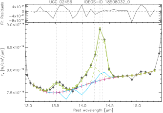
Figure 5: Example of a fit to the 13.05–15.40 $\mu$m spectrum of an IDEOS source. The observed spectrum is shown in black, and the fit to the data in green. Individual emission features are shown as green dashed curves on top of the local continuum (pink). Upper limits for undetected model features are overplotted in cyan. Vertical lines denote commonly detected features: 13.52 & 14.22$\mu$m PAH, 13.77$\mu$m C₂H₂, 14.02$\mu$m HCN, 14.32$\mu$m [Ne v], 14.37$\mu$m [Cl ii].

Our CHUNKFIT model for this range comprises the following spectral components:

• The 13–15.4 $\mu$m continuum, represented by a fourth order polynomial function. This continuum traces the onset of the 18 $\mu$m amorphous silicate feature, which may be in emission or absorption. In spectra with continuum S/N$<$13 at 14 $\mu$m we reduce the order of the polynomial continuum to second order.

• Emission lines of [Ne V] at 14.32 $\mu$m, and [Cl ii] at 14.37 $\mu$m, represented by Gaussian profiles.

• PAH emission bands at 13.52, and 14.22 $\mu$m, represented by Gaussian profiles.

• Absorption profiles of C₂H₂ at 13.7 $\mu$m and HCN gas at 14.0 $\mu$m (Lahuis et al., 2007), represented by Gaussian profiles. We do not attribute a physical meaning to this choice of profile, nor to the measured optical depth. See Lahuis et al. (2007) for a proper model fit.

High-resolution Spitzer-IRS studies of starburst galaxies have shown the [Cl ii] line to be faint, and therefore hardly detectable in SL and LL spectra (Bernard-Salas et al., 2009). Therefore, if our initial model fit indicates both [Cl ii] and [Ne v] to be detected, we omit [Cl ii] from the fitting parameters if [Ne v] represents at least 30% of the flux in the line blend, and then repeat the fit. Likewise, in case PAH142 is blended with [Ne v], we replace the detection of [Ne v] with an upper limit in case the flux ratio of [Ne v]/PAH142 is below a certain value. For spectra with continuum S/N$<$50 we choose 0.83, and for spectra with continuum S/N$>$50 it is 0.6. The above steps ensure that detections of 14.32 $\mu$m [Ne v] in IDEOS are true detections and not the result of misassignment of flux in a line blend. Of course, any redshift error on the order of 0.05$\mu$m ($\sim$1000 km/s) will result in all line flux to be assigned to just one of the lines in the blend.

3.5 Features in the 14.5–21 $\mu$m range

The 14.4–21 $\mu$m spectral range contains three diagnostically important emission lines, [Ne iii] at 15.56 $\mu$m, H₂ 0–0 S(1) at 17.03 $\mu$m, and [S iii] at 18.71 $\mu$m. Both the [Ne iii] and the [S iii] line are well-separated from other spectral features, unlike the H₂ 0–0 S(1) line, which, in star forming galaxies, sits atop a conglomerate of PAH features, the so-called 17 $\mu$m PAH complex (Smith et al., 2007). The 14.4–21 $\mu$m spectral range is also home to the O–Si–O bending vibration mode of amorphous silicates, which spans the entire range, and to the 16.1 and 18.6  $\mu$m absorption features due to crystalline silicates (Spoon et al., 2006).

Our CHUNKFIT model for this range comprises the following spectral components:

• The 14.5–21 $\mu$m continuum, represented by a fourth order polynomial function. This continuum traces the smooth shape of the 18 $\mu$m amorphous silicate feature, which may be either in emission or absorption.

• Emission lines of [Ne iii] at 15.56 $\mu$m, H₂ 0–0 S(1) at 17.03 $\mu$m, and [S iii] at 18.71 $\mu$m, represented by a Gaussian profile.

• PAH emission bands at 15.9, 16.45, and 17.4 $\mu$m, and a PAH plateau centered at 17.0 $\mu$m, all represented by Gaussian profiles.

• Absorption profiles of two crystalline silicate bands, at 16.1 and 18.6 $\mu$m, fitted together (see Appendix C and Fig. 32).

The 16.1 and 18.6 $\mu$m crystalline bands are only fitted in spectra that exhibit significant silicate absorption, S${}_{\rm sil}<-0.5$. This avoids unphysical solutions in spectra dominated by PAH emission bands. The bands are not fitted independent from each other as to limit the number of free parameters, to avoid unphysical fits to the amorphous silicate profile, and in recognition that their strengths appear correlated in deeply obscured sources (Spoon et al., 2006).

Fits to the spectra of two dusty star forming nuclei are shown in Fig. 6. Both plots highlight the remarkable good fit that the crystalline silicate template offers to almost all spectra of deeply obscured galactic nuclei.

As can be seen in the upper panel of Fig. 6, in spectra with a strong 17 $\mu$m PAH complex the accuracy of the line flux measured for the [Ne iii] line depends to some extent on the adopted profile for the 15.9 $\mu$m PAH band. Similarly, for spectra with crystalline silicate absorption the line flux of the [S iii] line is critically dependent on a good fit to the crystalline-absorbed continuum around the line. Note that our CHUNKFIT model does not include the line blend of [P iii] at 17.885 $\mu$m and [Fe ii] at 17.936 $\mu$m, because these lines are generally weak (Bernard-Salas et al., 2009), and because these added free parameters would decrease the degrees of freedom of the model to almost zero, similar to the model for the 5.39–7.25 $\mu$m range (Sect. 3.1).

In spectra with continuum S/N$<$7 at 17 $\mu$m we reduce the order of the polynomial continuum to third order, while in spectra with deep silicate absorption features we increase it by one order. Spectra that do not extend to at least 20.4 $\mu$m cannot be fitted with the model described above. For these spectra we perform a fit to just the 14.4–16.2 $\mu$m range to obtain a measurement of only the [Ne iii] line.

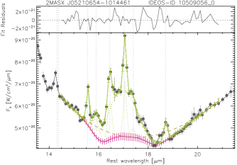
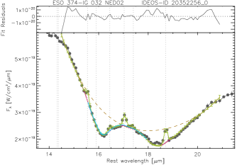
Figure 6: Fits to the 14.4–21 $\mu$m spectra of two IDEOS sources. In each fit the observed spectrum is shown in black and the fit to the data in green. The local continuum is plotted in pink, and the continuum corrected for crystalline silicate absorption in brown. Upper limits for undetected model features are overplotted in cyan. Vertical lines denote commonly detected features: 14.32$\mu$m [Ne v], 14.37$\mu$m [Cl ii], 15.56$\mu$m [Ne iii], 15.9$\mu$m & 16.45$\mu$m PAH, 17.03$\mu$m H₂ S(1), 17.40$\mu$m PAH, 18.71$\mu$m [S iii].

3.6 Features in the 19–36.5 $\mu$m range

The 19–36.5 $\mu$m spectral range is home to six emission lines of great diagnostic importance. Two of these are strongly blended in low-resolution spectra, [O iv] at 25.89 $\mu$m and [Fe ii] at 25.99 $\mu$m, at a separation of only $\sim$1100 km s^-1 peak to peak. The 19–36.5 $\mu$m range is devoid of strong emission and absorption bands from PAHs and amorphous silicates, but does exhibit features of crystalline silicates, either in emission or absorption, centered at 23.3, 27.5 and 33.2 $\mu$m (e.g. Spoon et al., 2006), characteristic of Forsterite, the magnesium-rich end member of the Olivines.

Our CHUNKFIT model for this wavelength range contains the following spectral components:

• The 19–36.5 $\mu$m continuum, represented by the following polynomial continuum in ln($\lambda/\lambda_{0}$) space: F($\lambda$) = $g$ exp[$a$ (ln [$\lambda/\lambda_{0}$]) + $b$ (ln [$\lambda/\lambda_{0}$])² + $c$ (ln [$\lambda/\lambda_{0}$])³ + $d$ (ln [$\lambda/\lambda_{0}$])⁴], where $\lambda_{0}$=25 $\mu$m. If the spectrum does not extend to at least 29.3 $\mu$m, d=0.

• Emission lines of [Ne v] at 24.32 $\mu$m, [O iv] at 25.89 $\mu$m, [Fe ii] at 25.99 $\mu$m, H₂ 0–0 S(0) at 28.22 $\mu$m, [S iii] at 33.48 $\mu$m, [Si ii] at 34.82 $\mu$m, and [Ne iii] at 36.01 $\mu$m, all represented by Gaussian profiles.

• Emission/absorption profiles of Forsterite, which has features at 23.2, 27.6, and 33.2 $\mu$m (see Appendix C and Fig. 32).

An example model fit is shown in Fig. 7 for a Seyfert galaxy exhibiting high-ionization lines and crystalline silicates in emission.

Given the small velocity separation of the [O iv] and [Fe ii] lines (1150 km s^-1; spectral resolution 3,000–4,000 km s^-1), a small error in the wavelength calibration or in the redshift of the source may lead to an incorrect distribution of the line flux between the two lines in the blend. Because of this, visual inspection of the model fit (Fig. 7) is advised before using the computed [O iv] and [Fe ii] line fluxes. Plots showing these model fits are available from the IDEOS portal (Sect. 10).

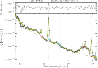
Figure 7: Example of a fit to the 19–35.5 $\mu$m spectrum of an IDEOS source. The observed spectrum is shown in black, the fit to the data in green. The local continuum is shown in pink, and the continuum corrected for crystalline silicate emission in brown. Upper limits for undetected lines are shown in cyan. Vertical lines denote commonly detected features: 24.32$\mu$m [Ne v], 25.89$\mu$m [O iv], 25.99$\mu$m [Fe iii], 28.22$\mu$m H₂ S(0), 33.48$\mu$m [S iii], and 34.82$\mu$m [Si ii].

3.7 Upper and lower limits for equivalent widths of PAH features

For three of the PAH features fitted by our CHUNKFIT models, PAH62, PAH11, and PAH127, we not only compute integrated fluxes but also equivalent widths. Below we describe how upper limits to the PAH flux and/or continuum flux affect the equivalent width that we report.

In case a PAH feature is not (significantly) detected (F_PAH$<$3$\sigma$), also its equivalent width becomes an upper limit. If, instead, the underlying continuum, C, is not significantly detected (C$<$3$\sigma$), the equivalent width becomes a lower limit. If both the local continuum and the PAH flux are not significantly detected, the equivalent width will be reported as undefined.

3.8 Compatibility of PAH flux measurements

PAH flux measurements resulting from the CHUNKFIT models presented in this section are compatible with PAH flux measurements from other methods in which the PAH feature flux is defined as the flux protruding above the local continuum. PAH profiles defined this way are approximately gaussian in shape at the resolving power of the IRS low-resolution modules.

In contrast, PAH flux and equivalent width measurements resulting from either the Lorentzian (Boulanger et al., 1998) or the Drude (Smith et al., 2007) PAH spectral decomposition method are not compatible with the aforementioned gaussian PAH profile assumption, as Lorentzian and Drude shaped profiles display far broader wings than gaussian profiles do, resulting in a PAH “continuum” underneath the local/apparent continuum. PAH flux and equivalent width measurements assuming Drude shape PAH profiles, resulting from spectral decomposition, are presented in Sect. 4. A comparison of the diagnostic powers of both kinds of PAH profile measurements is presented by Galliano et al. (2008b) and show the trends to be the same.

4 SED decomposition

We have performed spectral decomposition on all IDEOS SEDs with sufficient coverage of the main PAH complex (6–12 $\mu$m) to provide PAH flux and equivalent width measurements using the Drude profile PAH model. This provides access to a different set of PAH diagnostics in the literature than available for PAH measurements obtained using the gaussian PAH profile model (Sect. 3). For a comparison of both PAH models see Galliano et al. (2008b).

With the goal of avoiding unphysical decomposition solutions the implementation of the spectral decomposition differs depending on the nature of the mid-IR SED. For spectra showing the signatures of a buried source, i.e. ice, aliphatic hydrocarbon, and silicate absorption features (mid-IR classes 2A/B, 3A/B; Spoon et al., 2007), we used QUESTFIT (Veilleux et al., 2009), while for the remaining sources we used a modified version of PAHFIT (Smith et al., 2007). Both decomposition tools employ the same PAH profile shapes, thereby ensuring intercomparability of the PAH measurements between PAHFIT and QUESTFIT. Below we sketch the two decomposition methods in more detail.

4.1 SED decomposition using PAHFIT

We have used a modified version of PAHFIT (Gallimore et al., 2010) to measure the fluxes and equivalent widths of the main PAH emission bands in all but the most strongly obscured galaxies in the IDEOS sample. PAHFIT (Smith et al., 2007) uses MPFIT to find the best fitting combination of dust continua, stellar continuum, PAH emission bands, emission lines, and dust extinction for a given Spitzer-IRS low-resolution spectrum. The 24 PAH features in PAHFIT are represented by Drude profiles, which, given their close spacing and broad wings, produce a PAH “continuum” underneath their peaks.

The modifications to PAHFIT made by Gallimore et al. (2010) consist of a) excluding PAH and emission line features from extinction effects; b) adding an optically thin warm dust emission component; c) adding fine-structure emission lines of [Ne v] and $[$Ne vi$]$; d) widening the choice of extinction laws to include the cold dust model of Ossenkopf et al. (1992), in addition to Chiar&Tielens (2006) and an extinction law based on the silicate profile of Kemper et al. (2004).

To fit the spectra of a sample as diverse as the IDEOS sample we made further modifications to the fitting code. We removed the faint H₂ 0–0 S(4) and S(6) lines from the model. We raised the lowest allowed temperature for the optically thin warm dust emission component from 100 to 200 K to prevent an 18 $\mu$m silicate emission peak to be fitted by a cool dust black body component that peaks around 18 $\mu$m. We also removed from each individual PAHFIT model any emission line that was not previously detected as part of the CHUNKFIT fitting effort (Sect. 3). This reduces the number of free parameters at risk to be fitted to noise features or artefacts in low S/N spectra. Finally, we updated the spectral resolution table to reflect our adopted values (Table 2).

Depending on the sign of the silicate strength of the spectrum (Sect. 7), PAHFIT has either been run with the optically thin dust emission component switched on, and the extinction on the star light and dust continua switched off, or the opposite. This avoids run-away situations of silicate emission and absorption components reaching unphysical levels to cancel each other out in otherwise featureless spectra. Given the large differences in observed silicate emission profiles, for spectra with positive silicate strength we ran three PAHFIT models, each using a different choice of extinction law (see above) to represent the silicate emission features. We then chose the best fitting model based on the reduced $\chi^{2}$ of the fit. For silicate absorption spectra, we only used two of our extinction laws: Chiar&Tielens (2006) and Ossenkopf et al. (1992). Other than this, PAHFIT parameters were not tweaked to optimize fit results.

Given the large number of free parameters in any PAHFIT model, and the absence of constraints on the ratios between the 24 PAH components, there is nothing preventing PAHFIT from finding a best fitting solution in an unphysical part of parameter space. While this will not happen for PAH-dominated spectra, which PAHFIT was designed to fit, there is no straight-forward automated iterative way to identify unphysical fit results and then improve upon them. We therefore deem the PAH measurements from the CHUNKFIT fitting in Sect. 3 more robust, and provide the PAHFIT results only as a service.

4.2 SED decomposition using QUESTFIT

Because of the limitations of PAHFIT stated above, IDEOS spectra dominated by strong absorption features of silicates, ices and aliphatic hydrocarbons are not suitable candidates for spectral decomposition by PAHFIT. QUESTFIT (Rupke et al., 2021; Veilleux et al., 2009; Schweitzer et al., 2008), on the other hand, is tailored to the decomposition of deeply obscured sources, by including absorption by ices, aliphatic hydrocarbons, and crystalline silicates in the extinction model, and by limiting the number of free parameters governing the PAH contribution to just two: one per noise-free PAH emission spectrum included in QUESTFIT. We have therefore used QUESTFIT to measure the main PAH emission features of the almost 200 sources with mid-IR spectral classifications 2A/B, 3A/B (Spoon et al., 2007, see also Sect. 8.1) that are classified as buried sources.

Since the two noise-free PAH emission spectra used in QUESTFIT originate from PAHFIT (their templates 3 and 4; Smith et al., 2007), the PAH fluxes can be decomposed into Drude profiles, fully comparable with those computed for non-buried sources by PAHFIT. Note that emission lines are not fitted by QUESTFIT and are therefore masked out in the fitting process. QUESTFIT assumes all the extinction to occur in the nuclear continuum source, and the extinction in the circumnuclear star forming regions to be negligible (Veilleux et al., 2009). This is reflected in the reported PAH fluxes and equivalent widths.

4.3 Comparison of QUESTFIT and CHUNKFIT in the 5.5–8 $\mu$m range

For some deeply obscured sources, like the ULIRG IRAS F12127–1412NE, we find substantial differences between the spectral decomposition results of QUESTFIT and the CHUNKFIT model for the 5.39–7.25 $\mu$m range (Sect. 3.1). As can be seen in the top panel of Fig. 8, the continuum corrected for water ice and amorphous hydrocarbon absorption (the blue dashed line) lies significantly below the spline interpolated continuum (the red dashed line). The disparity appears to widen with increasing 5.5-8 $\mu$m wavelength. In contrast, the continuum components of the QUESTFIT spectral decomposition (bottom panel of Fig. 8) do provide a good overall fit to the 5.5–8 $\mu$m range (except for the depth of the 6.85 and 7.25 $\mu$m features; see below).

The striking disparity cannot be explained by differences in the profiles of the 5.5–8 $\mu$m absorption templates as these are not that different from each other (compare the optical depth profiles of NGC4418 and IRAS 08572+3915 in Fig. 29). Instead, we attribute the superior fit by QUESTFIT to a substantial contribution from a steeply rising continuum component devoid of ice and hydrocarbon absorption, and less affected by silicate absorption (bottom panel of Fig. 8). Could this be the spectral signature of a secondary nucleus? Or the effect of a much thinner, less frosty cocoon across part of the central source – a hole, if you will?

Inspection of the QUESTFIT result in the bottom panel of Fig. 8 further shows that the QUESTFIT model could be improved by fitting the aliphatic hydrocarbon component (the 6.85 and 7.25 $\mu$m features) separate from the rest of the adopted absorption profile, as is done in the CHUNKFIT model.

Further examples of galaxies with similarly unusual 5.5–8 $\mu$m optical depth profiles are IRAS 00188–0856, F10398+3247, 10485–1447, 13045+2353, F16156+0146NW, 17123–6245, 20100–4156 and 23515–2917. All of these galaxies require secondary continuum components in their QUESTFIT models that could be interpreted as signatures of less than full coverage of the source by ice and hydrocarbon absorptions.

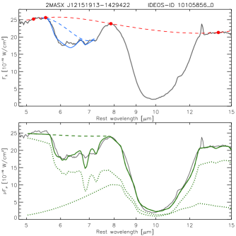
Figure 8: Comparison of fits to the 5.5–8 $\mu$m absorption features in the ULIRG IRAS F12127–1412NE. The upper panel shows the spline-interpolated local continuum in red (see Sect. 7.2), and our CHUNKFIT model for the 5.37–7.25 $\mu$m range (see Sect. 3.1) in blue. The 5.7–7.25 $\mu$m inferred continuum, corrected for ice and hydrocarbon absorption (see Sect. 3.1), is shown as a blue dashed line. Clearly, the two dashed continua are not in agreement. The lower panel shows the QUESTFIT spectral decomposition of the continuum (see Sect. 4.2) in green. The best fit to the 5.5–8 $\mu$m absorption features requires one ice and hydrocarbon absorbed component and one that lacks these features (dotted lines). The dashed green line is the implied absorption-corrected continuum, and is similar to the red dashed line in the upper panel.

5 Rest frame continuum flux densities

Sampling of the rest frame continuum at various near and mid-infrared wavelengths provides insight into the relative contributions of stellar photospheric and hot and cool dust emission to the galaxy spectrum.

We have used the IDEOS spectra to compute rest frame continuum flux densities at seven feature-free wavelengths in the 3.7 to 30 $\mu$m range: at 3.7, 4.2, 5.5, 15.0, 24.0, and 30.0 $\mu$m. All but the 3.7 and 4.2 $\mu$m rest frame fluxes are measured from the spectral fits for the wavelength ranges they are part of (Sect. 3). For the remaining two wavelengths the flux densities were computed in two steps. First, the average flux density in a narrow range of a few wavelength elements around the central wavelength was measured. Then a 1$\sigma$ clipping was performed after which the first step was repeated. The average flux density and the uncertainty in the mean are the final products.

We include the rest frame continuum flux density measurements in Table 8, along with two rest frame continuum flux density ratios: C(24 $\mu$m)/C(5.5 $\mu$m) and C(30 $\mu$m)/C(5.5 $\mu$m). Fig. 9 shows all rest frame continuum flux density measurements along with synthetic photometry for galaxy SBS 1648+547.

6 Synthetic photometry

The wide spectral range covered by the Spitzer-IRS low resolution spectra allows us to compute synthetic photometry for our sources in a large selection of IRAC, Spitzer, WISE and JWST-MIRI photometric bands.

We compute the synthetic photometric flux density as the photon-weighted mean flux density over the bandpass of the filter, where the normalization depends on the reference spectrum used for that filter.

For Spitzer-IRAC (Reach et al., 2005) and Spitzer-IRS the reference spectrum is a power law F${}_{\nu}(\nu)\sim\nu^{-1}$. The synthetic photometric flux density is thus defined as

$$\langle F_{\nu}(\lambda_{eff})\rangle=\frac{\int F_{\nu}(\nu)(\nu_{eff}/\nu)R(\nu)d\nu}{\int(\nu_{eff}/\nu)^{2}R(\nu)d\nu}$$ (1)

where $\lambda_{eff}$ is the effective wavelength of the photometric band, defined as:

$$\lambda_{eff}=c\frac{\int\nu^{-2}R(\nu)d\nu}{\int\nu^{-1}R(\nu)d\nu}=\frac{\int R(\lambda)d\lambda}{\int\lambda^{-1}R(\lambda)d\lambda}$$ (2)

and $R(\lambda)$=$R(\nu)$ is the filter transmission profile (in units of electrons per photon). For the IRAC-8, IRS-15 and IRS-22 photometric bands the effective wavelengths are 7.87, 15.8 and 22.3 $\mu$m, respectively.

For Spitzer-MIPS the reference spectrum is a T=10,000 K black body (Engelbracht et al., 2007), and thus the synthetic photometric flux density is defined as

$$\langle F_{\nu}(\lambda_{\rm 0})\rangle=\frac{\int F_{\nu}(\nu)(\nu_{\rm 0}/\nu)R(\nu)d\nu}{\int(\nu_{\rm 0}/\nu)(\frac{B_{\nu}(\nu,T=10^{4}\,K)}{B_{\nu}(\nu_{\rm 0},T=10^{4}\,K)})R(\nu)d\nu}$$ (3)

where $\lambda_{\rm 0}$=c/$\nu_{\rm 0}$ is defined as:

$$\lambda_{\rm 0}=\frac{\int c^{2}\nu^{-3}R(\nu)d\nu}{\int c\nu^{-2}R(\nu)d\nu}=\frac{\int\lambda R(\lambda)d\lambda}{\int R(\lambda)d\lambda}$$ (4)

resulting in $\lambda_{\rm 0}$=23.7 $\mu$m for the MIPS-24 band.

For WISE (Wright et al., 2010) the reference spectrum is a power law F${}_{\nu}(\nu)\sim\nu^{-2}$, and thus the synthetic photometric flux density is defined as

$$\langle F_{\nu}(\nu_{iso})\rangle=\frac{\int F_{\nu}(\nu)(\nu_{iso}/\nu)R(\nu)d\nu}{\int(\nu_{iso}/\nu)^{3}R(\nu)d\nu}$$ (5)

where $\lambda_{iso}$=c/$\nu_{iso}$ is the isophotal wavelength of the photometric band (Wright et al., 2010). For both band WISE-3 and WISE-4 discrepancies have been found between the pre-flight and on-sky performances, with red sources appearing too faint in band WISE-3 and too bright in band WISE-4 (Wright et al., 2010). Following Brown et al. (2014), we minimize the mismatch for WISE-4 by shifting the filter profile and isophotal wavelength upward by 3%, resulting in a revised isophotal wavelength of 22.8 $\mu$m. For band WISE-3 Wright et al. (2010) suggest that a 3–5% downward shift of the filter profile might minimize the mismatch in that filter band. Pending further investigation, we will adopt the pre-flight filter profile and isophotal wavelength of 11.56 $\mu$m for band WISE-3.

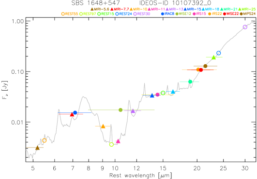
Figure 9: Synthetic photometry and rest frame continuum flux densities for galaxy SBS 1648+547. The horizontal bars indicate the wavelength ranges in which 80% of the filter transmission occurs. A legend is provided for the use of the symbols and color codes to distinguish the various photometric bands and rest frame flux densities.

For the MIRI Imager on the James Webb Space Telescope we adopt a T=5,000 K black body as the reference spectrum as proposed by Glasse et al. (2015). Thus the synthetic photometric flux density is defined as

$$\langle F_{\nu}(\nu_{\rm 0})\rangle=\frac{\int F_{\nu}(\nu)(\nu_{\rm 0}/\nu)R(\nu)d\nu}{\int(\nu_{\rm 0}/\nu)(\frac{B_{\nu}(\nu,T=5000\,K)}{B_{\nu}(\nu_{\rm 0},T=5000\,K)})R(\nu)d\nu}$$ (6)

where $\lambda_{\rm 0}$=c/$\nu_{\rm 0}$ is defined as in Eq. 5. The effective wavelengths for the MIRI filters as computed using Eq. 5 are tabulated in Table 5.

t Band name $\lambda_{eff}$ $\lambda_{p}$ MIRI-770 7.67 7.64 MIRI-1000 9.98 9.95 MIRI-1100 11.33 11.31 MIRI-1280 12.83 12.81 MIRI-1500 15.09 15.06 MIRI-1800 18.00 17.98 MIRI-2100 20.84 20.80 MIRI-2550 25.40 25.36

Table 5: Effective and pivot wavelengths for MIRI filters

Unlike the flux calibration methods employed by infrared astronomers, the HST method of flux calibration does not involve reference spectra, color corrections and effective wavelengths. The synthetic photometric flux density (Jy) is defined instead as a photon-weighted mean flux density over the bandpass of the filter (Koornneef et al., 1986; Bohlin et al., 2011):

$$\langle F_{\nu}\rangle=\frac{\int F_{\nu}(\nu)\nu^{-1}R(\nu)d\nu}{\int\nu^{-1}R(\nu)d\nu}$$ (7)

We have used this method to produce synthetic photometry for all nine bands of the JWST MIRI imager (Glasse et al., 2015). The results are included in Table 8. In lieu of an effective wavelength, which depends on the reference spectrum used, here we use the pivot wavelength $\lambda_{p}$ (Koornneef et al., 1986) to associate the synthetic photometric flux to the filter. The pivot wavelength is defined as

$$\lambda_{p}=\sqrt{\frac{\int\lambda R(\lambda)d\lambda}{\int\lambda^{-1}R(\lambda)d\lambda}}$$ (8)

and the results for the various MIRI filters are tabulated in Table 5.

7 9.8 $\mu$m silicate strength measurement

Following Spoon et al. (2007), we define the strength of the 9.8 $\mu$m silicate feature as:

$$S_{\rm sil}=\ln[f_{\nu}(\lambda_{\rm peak})/f_{\nu}^{\rm cont}(\lambda_{\rm peak})]$$ (9)

where f_ν($\lambda_{\rm peak}$) is the flux density of the spectrum at the peak of the silicate feature, $\lambda_{\rm peak}$, and f${}_{\nu}^{\rm cont}$($\lambda_{\rm peak}$) is the flux density of the underlying continuum at the same wavelength.

7.1 The observed 9.1-12.65 $\mu$m continuum

To determine the local continuum at $\lambda_{\rm peak}$, f_ν($\lambda_{\rm peak}$), we use MPFIT to model the spectral structure in the 9.1–12.65 $\mu$m range. For this we use the same approach as in Sect. 3.3, where we use the results of the first stage (10.0–12.65 $\mu$m) fit, to expand to a larger range that includes the H₂ 0–0 S(3) line at 9.66 $\mu$m and the continuum down to 9.1 $\mu$m. The wider wavelength range requires the use of a fourth order polynomial continuum, which is reduced to a third order polynomial continuum for spectra which are deemed noisy in the first stage fit. An example model fit is shown in Fig. 10.

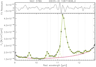
Figure 10: Example of a fit to the 9.1–12.58 $\mu$m spectrum of an IDEOS source. The observed spectrum is shown in black, and the fit to the data in green. Individual emission features are shown as green dashed curves on top of the local continuum (pink). Vertical dotted lines denote commonly detected features: 9.66$\mu$m H₂ S(3), 10.51$\mu$m [S iv], 10.64, 11.04, 11.29, 11.98$\mu$m PAH, and 12.28$\mu$m H₂ S(2).

7.2 The underlying continuum

The underlying continuum f${}_{\nu}^{\rm cont}$ is an estimate of what the flux density of the spectrum would be in absence of silicate emission or absorption. This is a somewhat subjective measurement that depends on our assumption on how the underlying continuum varies with wavelength between ”anchor” points sufficiently far from the silicate feature to be unaffected by it. The most common choices are either a spline or a power-law interpolation.

The diversity among the mid-infrared spectra in IDEOS implies that none of these interpolation methods provides optimal results in all cases. We find that spline interpolation produces more realistic underlying continua in sources with little or no PAH emission, but power-law interpolation is more robust in sources with stronger PAH bands. We hence compute S${}_{\rm sil}^{\rm spline}$ and S${}_{\rm sil}^{\rm powerlaw}$ for all sources and define the sample of sources with strong PAH emission to be characterized by EQW(PAH11) $>$0.1 $\mu$m and S${}_{\rm sil}^{\rm powerlaw}$$>$-2. The latter condition ensures that sources with weak PAH11 emission and weak 11.25 $\mu$m continuum emission, resulting from strong silicate absorption, are not included with sources that have EQW(PAH11)$>$0.1 $\mu$m due to strong PAH emission. For the power-law interpolation we need two anchors that are placed at 5.5 and 14.0 $\mu$m (Spoon et al., 2007). See Fig. 11. For the spline interpolation we take anchor points at several additional wavelengths: 7.0, 26.5, and 31 $\mu$m. See Fig. 12. For sources with insufficient spectral coverage at long wavelengths we replace the last two anchors by 25.0 and 28.0 $\mu$m, or 23.0 and 25.5 $\mu$m. If the spectral coverage does not even reach 25.5 $\mu$m, we replace the 14.0 $\mu$m anchor by two at 13.5 and 15.0 $\mu$m. For deeply obscured sources, like NGC 4418 shown in Fig. 13, an additional anchor around 5 $\mu$m becomes necessary, while the anchor at 7.0 $\mu$m is replaced by an anchor at 7.8 $\mu$m.

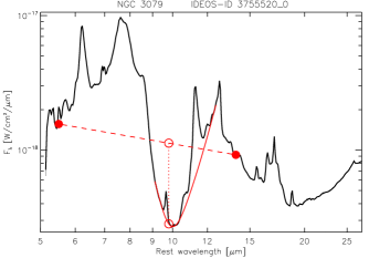
Figure 11: Example of a power-law fit to the local continuum in the 5–14 $\mu$m range to determine the underlying continuum f${}_{\nu}^{\rm cont}$ (dashed red line) in the 8–14 $\mu$m range. Given that the 10 $\mu$m silicate feature is in absorption, the silicate strength S${}_{\rm sil}^{\rm powerlaw}$ is assessed at 9.8 $\mu$m. The red continuous line is the local continuum, f_ν, resulting from the MPFIT model for the 9.1–12.65 $\mu$m range described in Sect. 7.1.

Among the 2847 sources where the silicate feature is observed there are 616 sources for which the spectral coverage or SNR is insufficient to obtain either the 5.5 or the 14.0 $\mu$m (13.5 and 15.0 $\mu$m for splines) anchors from the spectrum. We found that moving any of these anchors closer to the silicate feature can bias the results significantly, so we chose instead to estimate the flux density at 5.5 and 14.0 $\mu$m by fitting the spectrum with a model that spans the 5–16 $\mu$m range, and then measure the missing anchor fluxes on the model. For this purpose we use deblendIRS (Hernán-Caballero et al., 2015). The deblendIRS model uses only three physical components (stellar, ISM and AGN), each of them represented by an empirical template selected from a large library of observed spectra). The best-fitting deblendIRS model reproduces the observed spectra with high accuracy (typical reduced $\chi^{2}\sim$1), and spans the 5–16 $\mu$m range irrespective of the wavelength coverage of the original spectrum. To estimate the uncertainty in the extrapolation of the spectrum using the deblendIRS mode, we have compared in a random sample of 500 sources with sufficient spectral coverage and high S/N the actual fluxes at 5.5 and 15.0 $\mu$m with those obtained from the deblendIRS model when the fitting range is reduced to 7.0–16.0 $\mu$m and 5.0–12.0 $\mu$m, respectively. In both cases we obtain a 1-$\sigma$ dispersion of 25%, with no significant bias.

The default anchor points for the spline or power law methods provide realistic underlying continua for most sources, but fail in the cases where the continuum has an unusual shape, like deeply obscured ULIRGs or quiescent galaxies, whose MIR spectra are dominated by the Rayleigh-Jeans tail of the stellar emission. For these sources we adjust manually the anchor wavelengths until a realistic continuum is obtained.

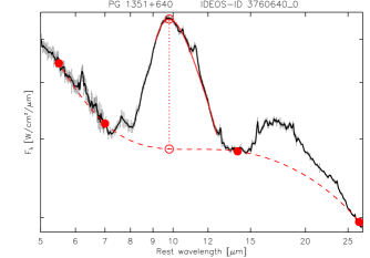
Figure 12: Example of a spline fit to the local continuum in the 5–26 $\mu$m range to determine the underlying continuum, f${}_{\nu}^{\rm cont}$, (dashed red line) valid for the 8–20 $\mu$m range. Given that the silicate features in this source are in emission, the silicate strength S${}_{\rm sil}^{\rm spline}$ would normally be assessed at 10.5 $\mu$m. Here we assess it at 9.8 $\mu$m, where visual inspection shows the peak to reside. The red continuous line is the local continuum, f_ν, resulting from the MPFIT model for the 9.1–12.65 $\mu$m range described in Sect. 7.1.

7.3 Shape of the 9.8 $\mu$m silicate profile

When the silicate feature appears in absorption it always peaks at $\sim$9.8 $\mu$m. However, when in emission the peak is often broad and displaced to longer wavelengths. Hatziminaoglou et al. (2015) reported that in a large sample of AGN, the peak of the silicate feature, when observed in emission, is at $\lambda$$>$10.2 $\mu$m in 65% of cases and at $\lambda$$>$10.6 $\mu$m in 20%. The exact peak wavelength of the broad silicate emission feature depends on the definition of the underlying continuum, on the representation chosen ($f_{\nu}$, $\nu f_{\nu}$, or $f_{\lambda}$), the temperature distribution of the dust and composition of the emitting silicates, and, in low SNR spectra, on the random noise in the spectrum.

It therefore matters what peak wavelength $\lambda_{\rm peak}$ is chosen. To have a robust method that works also for low S/N spectra, for silicate features found in absorption we will assume $\lambda_{\rm peak}$ to be at 9.8 $\mu$m. When found in emission we will use 10.5 $\mu$m, unless visual inspection shows the peak to be at 9.8 $\mu$m (e.g. PG1351+640 in Fig. 12). We interpolate the fitted 9–12.6 $\mu$m continuum and the underlying continuum to $\lambda_{\rm peak}$ to obtain f_ν($\lambda_{\rm peak}$) and f${}_{\nu}^{\rm cont}$($\lambda_{\rm peak}$), and using Eq. 9, S_sil.

Figure 13: Example of a spline fit to the local continuum of a deeply obscured source, NGC 4418. Given the steep upturn at the shortest wavelengths and the presence of a deep ice and aliphatic hydrocarbon absorption complex in the 7 $\mu$m range, an additional anchor point is needed at $<$5.5 $\mu$m and the 7 $\mu$m anchor point has to be shifted to 7.8 $\mu$m. See Fig. 12 for further details.

7.4 Uncertainties

We estimate the statistical uncertainty in S_sil using a Monte Carlo method. For every spectrum we obtain 50 copies, where gaussian noise has been added to each pixel consistent with its flux uncertainty. We re-evaluate the underlying continuum and the fitted 9–12.6 $\mu$m continuum that best fits the silicate feature for each of these copies, and measure S_sil in all of them. We then calculate the uncertainty in S_sil as the standard deviation of the values obtained for the 50 copies.

In sources with noisy spectra or very deep silicates, the flux of the fitted 9–12.6 $\mu$m continuum at $\lambda_{\rm peak}$ is sometimes less than zero. For these sources we use the distribution of S_sil values in the 50 copies to give an upper limit for S_sil at the 95% confidence level.

While the Monte Carlo method gives realistic statistical uncertainties for a given continuum interpolation method, it is important to keep in mind that the main uncertainty in the silicate strength may be systematic in nature, associated with the choice of interpolation method, or from the need to invoke deblendIRS. Analysis of the silicate strength solutions from the spline and powerlaw methods at the boundary of their validity ranges quantifies the systematic uncertainty as 0.2 in silicate strength.

8 Diagnostic plots

8.1 Mid-Infrared spectral classification

Before the advent of Spitzer-IRS the study of spectral features in galaxy spectra was limited to low-resolution spectra in the 5–11 $\mu$m range (ISO-PHT-S) and 5–16 $\mu$m range (ISO-CAM-CVF) plus targeted high spectral resolution line observations between 2 and 45 $\mu$m (ISO-SWS). Spitzer-IRS openend up the 5–37 $\mu$m range for full range spectroscopy of thousands of galaxies in the Local Universe. This enabled for the first time the use of the 9.8 $\mu$m silicate feature as an obscuration diagnostic without the limitations imposed by the inability to properly define a local 5–14 $\mu$m continuum both in spectra obtained on the ground and from space. The ’silicate strength’, first defined in 2006, was subsequently used by Spoon et al. (2007) to classify galaxies based on their location in the diagram that separates galaxies by the equivalent width of the 6.2 $\mu$m PAH feature (EQW62) and the silicate strength (S_sil).

Fig. 14 shows the distribution of 2524 IDEOS galaxies, color-coded by redshift bracket, over this diagram. Galaxies appear to be confined within a wedge-shaped region demarkated by two prongs of a fork and three vertices:

• In the lower right we find galaxies dominated by exposed star formation, as evidenced by strong PAH emission. The 9.8 $\mu$m silicate feature is weakly in emission or absorption.

• In the lower left we find galaxies dominated by AGN-heated hot dust. These galaxies show very little or no sign of PAH emission (star formation) and show only weak silicate emission or absorption.

• In contrast, galaxies in the upper left are dominated by deep absorption features of silicates. PAH emission features (the tell-tale signatures of exposed star formation) are generally faint or absent. Since the presence of deep silicate absorption features requires a strong negative temperature gradient in the dust along our line of sight (e.g. Sirocky et al., 2008) and full and optically thick coverage of the power source, the power source in these galactic nuclei must be compact: either an ultra-compact nuclear starburst or a supermassive black hole, hidden in a dust cocoon or at the center of an edge-on torus.

The large differences in spectral appearance of galaxies found in between these vertices makes a galaxy classification scheme based on silicate strength and PAH62 equivalent width useful.

Following Spoon et al. (2007), we have classified the IDEOS spectra into a grid of 3-by-3 classes based on the measured ice-corrected PAH62 equivalent width and the silicate strength. The classes range from 1A to 3C and are overlaid in Fig. 14. Even though this classification scheme is based on just two mid-infrared observables, it better captures the essential differences among infrared galaxies than any of the other 2-dimensional mid-infrared diagnostic diagrams shown in subsequent figures (Figs. 15–20).

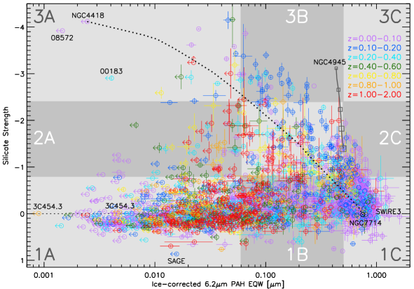
Figure 14: Diagnostic diagram combining the ice-corrected equivalent width of the 6.2 $\mu$m PAH feature (Sect. 3.1) with the silicate strength (Sect. 7). The 2524 galaxies are color-coded by redshift. Also included are several Spitzer-IRS mapping spectra of NGC 4945, centered on the deeply buried AGN and integrated over areas ranging from 5.5$"$$\times$5.5$"$ to 76$"$$\times$31.5$"$, with the symbol size proportional to the area. The diagram is subdivided in nine named quadrants, which form the basis of our mid-infrared galaxy classification scheme. Galaxies in class 1A have a hot dust-dominated spectrum typical for AGN. Galaxies in class 1C have PAH-dominated spectra typical for starburst galaxies. Galaxies in class 3A have absorption-dominated spectra typical for centrally heated dust shells or tori. Galaxies in between these extremes show intermediate properties. The dotted line shows the mixing line of galaxies with spectra intermediate between those of NGC 4418 and NGC 7714. In the plot the label SAGE refers to SAGE1C J053634.78–722658.5, SWIRE to SWIRE3 J105056.08+562823.0, 00183 to IRAS F00183–7111, 08572 to IRAS 08572+3915N. Galaxy 3C454.3 appears twice, in its high and low states as discussed in the text.

The large majority of the galaxies in this ’Fork Diagram’ (84%) are scattered along the horizontal branch of the fork, which connects classes 1A and 1C. Active galaxies with a Seyfert optical classification are generally confined to classes 1A and 1B, and the strongly AGN-dominated galaxies to class 1A. Starburst galaxies are home to classes 1C, with the more dust enshrouded ones showing up in class 2C (e.g. M82). Normal star forming galaxies, with spectra similar to the four noise-free template spectra of Smith et al. (2007), are found in class 1B (just over the border from class 1C) thanks to a stronger contribution of stellar photospheric emission to the 6.2 $\mu$m continuum underneath the 6.2 $\mu$m PAH feature. 14% of the galaxies in the Fork diagram are distributed over classes 2B/2C/3A/3B, which, together with class 1C, form its diagonal prong, and which is demarcated by the dashed line in Fig. 14 that represents the mixing line between the spectra of the buried nucleus of NGC 4418 and the starburst galaxy NGC 7714. Only 2% of the galaxies in the Fork Diagram are found in class 2A, in between the two prongs of the fork. Compared to the galaxies in class 3A, above them, their spectra show shallower silicate absorption features. These shallower silicate features are most easily explained as resulting from dilution of the absorption spectrum by continuum emission, either resulting from key hole openings in a dust cocoon (Marshall et al., 2018), or from a glimpse into the central region of a dust torus seen at an intermediate inclination (Rowan-Robinson et al., 2009, A. Efstathiou priv. comm.).

Classic galaxy evolution scenarios (Sanders & Mirabel, 1996; Hopkins et al., 2006) predict merging galaxies to go through a phase of strong nuclear obscuration before a naked AGN emerges. In this scenario two normal star forming galaxies would thus start their journey together in class 1C (or just across the border in class 1B), make their way up in the Fork Diagram, before descending and ending up as a merged class 1A AGN. The large majority of IDEOS galaxies found in classes 2A-3B are indeed caught as LIRGs and ULIRGs in interaction (Armus et al., 2020, and references there in).

With a sample of 2524 galaxies at hand it is interesting to point out some interesting, in certain aspects extreme, sources in the Fork Diagram:

• The galaxy with the highest silicate strength (S_sil=0.865 is SAGE1C J053634.78-722658.5. The galaxy was discovered in a survey of the Large Magellanic Cloud, and has an infrared spectrum completely devoid of cold dust emission associated with star formation (Hony et al., 2011; Van Loon et al., 2015) and has hence been referred to as a naked AGN.

• The galaxy with the lowest EQW62 is the blazar 3C 454.3. Spitzer-IRS observed the galaxy 31 times between June 30, 2005 (only weeks after the historic outburst of early May 2005; Fuhrmann et al., 2006), and January 23, 2009, during which the upper limit for PAHEQW62 reached a lowest value of 9$\times$10^-4 $\mu$m on July 7, 2005. This event coincides with the highest measured 5.5 $\mu$m continuum flux density of 516 mJy, which is 30 times higher than its lowest measured value of 17 mJy on January 24, 2009. The slope of the powerlaw spectrum, as measured from the 3.7 to 15 $\mu$m continuum flux ratio ranged from 0.14 to 0.25 in these 4.5 years.

• The most deeply buried galaxies with the, by far, tightest upper limits for the presence of PAH62 emission are NGC4418 (Spoon et al., 2001) and IRAS 08572+3915NW (Spoon et al., 2006) at S_sil -4.12, and -3.92, and PAH62EQW$<$2.5$\times$10^-3 $\mu$m and $<$1.5$\times$10^-3 $\mu$m, respectively. Both galaxies are interacting, but neither is in the final stages of coalescence. NGC 4418 is connected to VV 655 by a 50 kpc gas bridge (Varenius et al., 2017), and IRAS 08572+3915NW has a projected nuclear separation of 6 kpc to IRAS 08572+3915SE (Colina et al., 2005). Deep silicate features can hence not be relied on as sign posts for the very final stages of a merger.

• At a distance of 3.7 Mpc, NGC 4945 is the nearest galaxy hosting a deeply buried AGN. Our line of sight into the nucleus shows a wealth of ice absorption features (Spoon et al., 2000, 2003), some of which (e.g. the 15 $\mu$m CO₂ ice absorption feature (Peréz-Beaupuits et al., 2011)) have not been detected in any other galaxy thus far. Within the IDEOS sample NGC 4945 is unique for showing a strongly absorbed PAH emission spectrum rather than a strongly absorbed continuum spectrum at the position of the AGN (Peréz-Beaupuits et al., 2011). This places the nucleus proper in an otherwise unpopulated section of the Fork Diagram. Thanks to the availability of a Spitzer-IRS-SL map of the central 76$"$$\times$31.5$"$ (1.37kpc $\times$ 0.57kpc; PI: H.W.W. Spoon), it is possible to quantify the effect of including a larger and larger portion of the circumnuclear starburst ring and the galaxy disk in an extraction aperture. As shown in Fig. 14, the galaxy spectrum moves from class 3B to 2B and 2C as the nuclear absorption spectrum gets more and more overwhelmed by a PAH emission spectrum associated with unobscured/exposed star formation from the galaxy disk. The spectrum of NGC 4945 as a whole would likely be classified as a class 1C starburst spectrum. The example of NGC 4945 illustrates to what extent the physical projected size associated with the Spitzer-IRS SL slit differs between nearby and distant galaxies: at z=0.05, the SL slit only includes the central 3 kpc of a galaxy. Galaxies shown in purple in Fig. 14 are thus repesented by their nuclear properties.

• The highest redshift galaxy with a pure starburst spectrum in the fork diagram is SWIRE3 J105056.08+562823.0 (z_IRS=1.537) at S_sil=-0.32 and PAH62EQW=1.01 $\mu$m. The source is labeled ’SWIRE3’ in the diagram.

8.2 Mid-Infrared continuum slope diagnostics

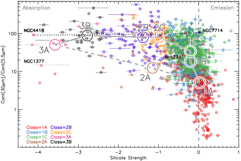
Figure 15: Diagnostic diagram of the 30 $\mu$m to 5.5 $\mu$m continuum ratio versus the 9.8 $\mu$m silicate strength. Large open circles denote the median locations of each of the mid-IR classes (Sect. 8.1) in the diagram. The gray lines connecting classes 1C to 1A and 1C to 3A trace the two branches of the Fork Diagram (Fig. 14). The dashed gray line show the effect of a change in silicate strength on sources that lack PAH contamination (Mid-IR classes 1A, 2A and 3A). The dotted black line is the mixing line between the spectra of NGC 4418 and NGC 7714.

Our measurements of the rest frame continuum flux densities at various mid-infrared wavelengths allow us to use the ratio of warm 30 $\mu$m to hot 5.5 $\mu$m rest frame continuum emission as an additional diagnostic. Exactly what the diagnostic power entails depends on the adopted dust geometry around the heating sources:

• A galactic nucleus hidden within a dust shell will see a decrease in the C(30 $\mu$m)/C(5.5 $\mu$m) ratio as the column density of the dust shell decreases.

• A decrease in the covering factor of the obscuring shell around a galactic nucleus (the emergence of a “keyhole”) will result in the decrease of the C(30 $\mu$m)/C(5.5 $\mu$m) ratio (Marshall et al., 2018).

• A change in orientation of a non-clumpy torus from edge-on view to pole-on view will result in a decrease of the C(30 $\mu$m)/C(5.5 $\mu$m) ratio (Rowan-Robinson et al., 2009, A. Efstathiou priv. comm.).

Fig. 15 shows the distribution of the IDEOS sources in a diagram of the C(30 $\mu$m)/C(5.5 $\mu$m) ratio versus the silicate strength. Like in the Fork Diagram the majority of the galaxies are found along two almost ortogonal branches. The vertical branch comprises sources that range from AGN to starburst galaxies (i.e. sources on the horizontal branch in the Fork Diagram: classes 1A–1B–1C), whereas sources on the horizontal branch are sources that range from enshrouded nuclei without significant circumnuclear star formation to starburst galaxies with dusty nuclei (i.e. sources on the diagonal branch in the Fork Diagram: classes 3A–3B–2B–2C–1C).

The dashed gray line shows the effect that a change in silicate strength would have on the continuum slope for galaxies with similar low levels of spectral contamination by PAH emission (i.e. mid-IR classes 1A–2A–3A). As can be seen in Fig. 15, decreasing the obscuration results in a decrease of the C(30 $\mu$m)/C(5.5 $\mu$m) ratio.

Taken at face value, it is remarkable that the median C(30 $\mu$m)/C(5.5 $\mu$m) ratio of the IDEOS sources hovers around 50–100 over a large span in silicate strength (-4 to -1) along the horizontal branch (classes 3A–3B–2B–2C–1C). Apparently, the increase in 5.5 $\mu$m continuum emission afforded by a lower obscuration level is compensated for by an increase in warm 30 $\mu$m continuum emission associated with an increased contribution of exposed star formation along this branch.

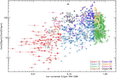
Figure 16: The circles denote the median locations of each of the mid-IR classes (Sect. 8.1) in the diagram. The gray connecting lines trace the two branches of the Fork Diagram (Fig. 14). The dashed gray line show the effect of a change in silicate strength on sources that lack PAH contamination (Mid-IR classes 1A, 2A and 3A).

Fig 16 is an adaptation of the Laurent Diagram (Laurent et al., 2000; Peeters et al., 2004), using the wider wavelength coverage of Spitzer-IRS. The Laurent Diagram was originally devised to quantify the contribution from AGN, PDR and HII regions to a galaxy spectrum by delineating the PAH62 equivalent width and the 5–15 $\mu$m continuum slope. Buried nuclear activity was not considered back then, as there were very few galaxies for which the 9.8 $\mu$m silicate feature could be observed (Peeters et al., 2004).

The diagram separates classic AGNs (mid-IR class 1A) and starburst galaxies (mid-IR class 1C) into opposite corners. The diagonal thick gray line in the diagram connects these two extremes. The diagram is, however, less successful in separating out galaxies dominated to varying degrees by buried nuclear activity (mid-IR classes 3A-3B-2B-2C-1C). Both the Fork Diagram (Fig 14) and the continuum slope versus silicate strength diagram (Fig. 15) do this far more effective.

8.3 Mid-Infrared ionized gas excitation diagrams

The mid-infrared fine-structure lines of ionized neon gas form an excellent diagnostic for the excitation of the ionized gas. The lines, [Ne ii] at 12.81 $\mu$m, [Ne iii] at 15.6 $\mu$m, [Ne v] at 14.32 & 24.32 $\mu$m, and [Ne vi] at 7.65 $\mu$m, span a range of ionization potentials (21, 41, 97, and 127 eV), have critical densities $>$10^4.5 cm^-3, do not suffer from strong differential extinction (due to amorphous silicate resonances), and are insensitive to abundance uncertainties.

In our galaxy [Ne v] and [Ne vi] emission is detected only from shocks associated with supernova remnants (e.g. RCW 103; Oliva et al., 1999). Their combined signal is not strong enough to be detectable in nuclear or galaxy-integrated spectra like ours (Peréz-Beaupuits et al., 2011). The detection of [Ne v] in an IDEOS spectrum is hence a tell-tale sign for the presence of an AGN. The inverse is not true, the absence of a [Ne v] line detection does not mean that an AGN is absent, as strong extinction in the line of sight to the narrow line region will decrease its equivalent width. The number of [Ne v] detections (either at 14.32 or 24.32 $\mu$m) in our sample is 390. Thus, at least 390/3335 galaxies in our sample host an AGN.

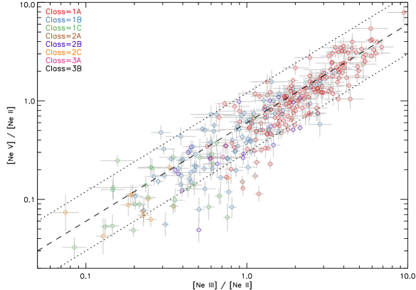
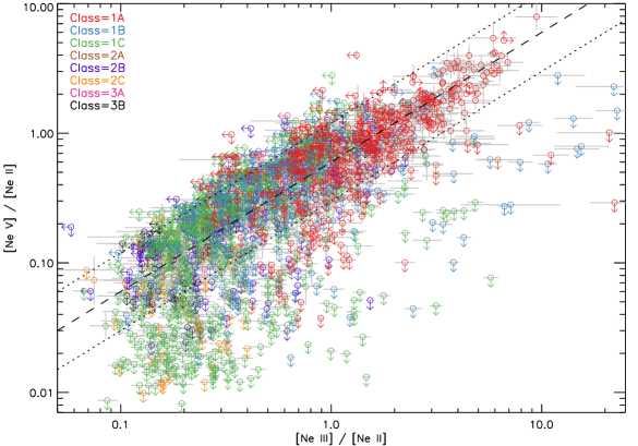
Figure 17: Excitation diagram of ionized neon gas based on the 12.81 $\mu$m [Ne ii], 15.56 $\mu$m [Ne iii], and 14.32 $\mu$m [Ne v] lines. In the upper panel we include just the 316 sources with detections for all three lines, whereas in the bottom panel we also include the 1312 sources for which one or both ratios are upper or lower limits. The dashed line indicates [Ne v]/[Ne iii]=0.6, and the dotted lines a ratio of 0.3 and 1.2, respectively. The galaxies are color-coded by mid-infrared galaxy class as defined in Sect. 8.1. Drop-out sources found in the quadrant defined by [Ne iii]/[Ne ii]$>$1 and [Ne v]/[Ne iii]$<$0.3 correspond to the low-metallicity sources found on the horizontal branch in Fig. 18.

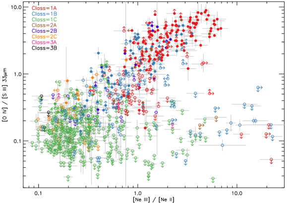
Figure 18: Excitation diagram based on the 12.81 $\mu$m [Ne ii], 15.56 $\mu$m [Ne iii], and 25.89 $\mu$m [O iv] and 33.48 $\mu$m [S iii] lines. 692 galaxies are plotted. Bonafide AGN, as confirmed by a detection of a [Ne v] line, are shown as filled circles. The galaxies are color-coded by mid-infrared galaxy class as defined in Sect. 8.1.

In the upper panel of Fig. 17 we show the positions of 316 sources that have detections for all three neon lines, 12.81 $\mu$m [Ne ii], 15.56 $\mu$m [Ne iii], and 14.32 $\mu$m [Ne v]: all of them bonafide AGN. The source distribution is best described by a linear relation characterized by [Ne v]/[Ne iii]=0.6, in good agreement with the results of Gorjian et al. (2007) for a sample of Seyferts and 3C radio sources. As the color-coding of the sources suggest, the highest excitation AGNs have a mid-IR classification 1A (low PAH equivalent width and only weak silicate emission/absorption), whereas the lowest excitation AGNs are found among class 1C and 2C galaxies (dominated by a PAH emission spectrum). Intermediate [Ne v]/[Ne ii] ratios are found among class 1B and 2B sources. The highest excitation source in our sample, as inferred from the [Ne v]/[Ne ii] ratio, is the nearby radio galaxy 3C 321. Its ([Ne iii]/[Ne ii] ratio is 9.4 and its [Ne v]/[Ne ii] ratio is 7.9.

In the lower panel of Fig. 17 we also include upper and lower limits for the line ratios, bringing the total source count in the plot to 1628. Some of the upper limits for [Ne v]/[Ne ii] are clearly inconsistent with membership of the diagonal band seen in the upper panel. We identify these “drop outs” in the quadrant defined by [Ne iii]/[Ne ii]$>$1 and [Ne v]/[Ne iii]$<$0.3 (the lower dotted line in Fig. 17) with the low-metallicity galaxies found in Fig. 8 of Hao et al. (2009). Among them are well-known sources like Haro 11, NGC 1140, Mrk1450, Mrk1499, and II Zw 40. Included among the drop outs are also Wolf-Rayet galaxies like IRAS 11485–2018. Note that some of these galaxies have [Ne iii]/[Ne ii] ratios exceeding those for the most extreme AGNs by a factor 2 or more. For example IRAS 11485–2018: [Ne iii]/[Ne ii]=22$\pm$6.

Following Hao et al. (2009), in Fig. 18 we plot the [Ne iii]/[Ne ii] ratio versus the [O iv]/[S iii] 33 $\mu$m ratio. This separates galaxies with Blue Compact Dwarf (BCD) properties along a horizontal “drop out” branch from galaxies which range from starburst to AGN dominated on a diagonal branch. We identify the galaxies on the horizontal branch with the “drop out” sources in Fig. 17. Clearly, [O iv]/[S iii] 33 $\mu$m does a better job at separating the low-metallicity drop-outs from other sources than [Ne v]/[Ne ii] does. Note that, like in Fig. 17, the [Ne iii]/[Ne ii] ratio reaches higher values among the galaxies on the horizontal branch than among galaxies on the diagonal branch.

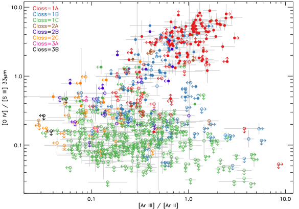
Figure 19: Excitation diagram based on the 6.99 $\mu$m [Ar ii], 8.99 $\mu$m [Ar iii], 25.89 $\mu$m [O iv], and 33.48 $\mu$m [S iii] lines. 565 galaxies with measurements for all four lines are plotted. Bonafide AGN, as confirmed by a detection of a [Ne v] line, are shown as filled circles. The galaxies are color-coded by mid-infrared galaxy class as defined in Sect. 8.1.

For galaxies at redshifts above 1.2 all three neon lines used in the diagnostic diagram of Fig. 17 are redshifted out of the JWST-MIRI range. The only bright mid-infrared fine-structure lines left to probe the hardness of the radiation field are the 6.99 $\mu$m [Ar ii], the 8.99 $\mu$m [Ar iii] and the 7.65 $\mu$m [Ne vi] lines. These three lines can be detected with MIRI up to z=2.2.

To assess whether the [Ar iii]/[Ar ii] ratio by itself suffices as an AGN/starburst diagnostic, in Fig. 19, we plot the [Ar iii]/[Ar ii] ratio versus the [O iv]/[S iii] ratio. Like in Fig. 18, galaxies are distributed along two prongs of a fork. The upper diagonal branch is populated with sources hosting an AGN, whereas the horizontal/downward tipping branch we find star forming galaxies and low-metallicity galaxies. This separation is clearer than in the previous two diagnostic diagrams where most class 1C galaxies are found at the bottom end of the diagonal branch along with the active galaxies higher up. It is clear that, without measurement of the 7.65 $\mu$m [Ne vi] line (or coronal lines at shorter mid-infrared wavelengths), it is impossible to determine from the [Ar iii]/[Ar ii] ratio alone whether the galaxy is an AGN-starburst composite or purely star formation powered. The argon line ratio by itself (just like the [Ne iii]/[Ne ii] ratio) is thus not a good AGN/starburst diagnostic.

9 Crystalline silicates

9.1 Crystalline silicate inventory

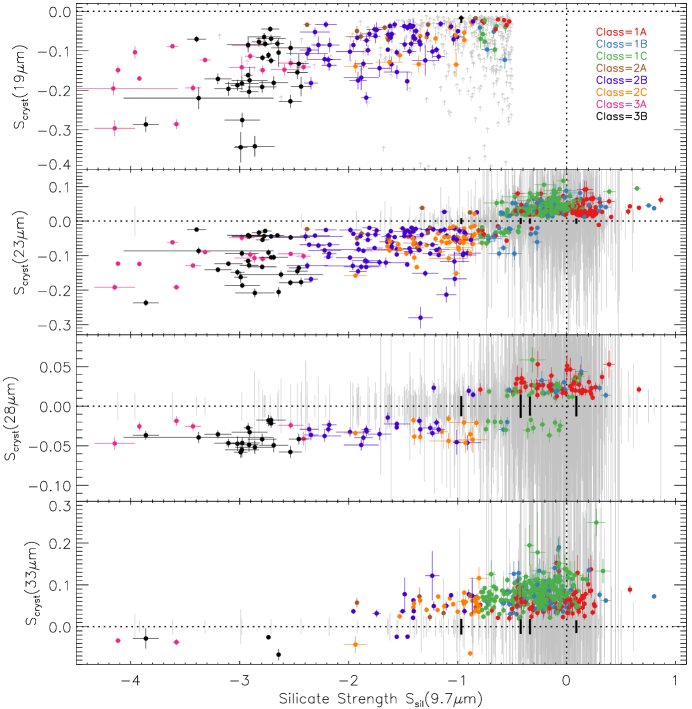
Figure 20: Strength of four crystalline silicate bands as a function of the 9.7 $\mu$m amorphous silicate strength. Detections of the crystalline bands are shown as filled circles, non-detections in gray and black. Since the 16 and 19 $\mu$m bands are fitted as absorption features, and only in spectra with S_sil$<$-0.5 (see Sect. 3.5), a non-detection of the 19 $\mu$m crystalline silicate band is marked by a gray upward arrow. The 23, 28 and 33 $\mu$m crystalline silicate bands, on the other hand, are allowed to be in emission or absorption (Sect. 3.6). Non-detections of these bands are shown as gray vertical bars stretching from -3$\sigma$ to +3$\sigma$. The non-detections shown in black identify four sources (2MASS J19563578+1119050 at S_sil=-0.97, ESO 239-IG 002 at S_sil=-0.42, II Zw40 at S_sil=-0.34, and 3C 390.3 at S_sil=0.09) that show no trace of crystalline silicate features at any wavelength.

As part of our SED fitting (Sect. 3), we have detected at a $>$95% confidence level emission and absorption features of crystalline silicates in 786/3335 IDEOS galaxies. These detections range from detections of a single band to detections of all five fitted bands in the 16–34 $\mu$m range. We find the detections not to be limited to a specific galaxy population. Crystalline silicates are, for instance, detected in low-metallicity galaxies (e.g. Haro 11), but also in quasars (e.g. 3C 273), and in at least one early-type galaxy, NGC 1209.

We define the crystalline silicate strength in the same way as the strength of the 9.8 $\mu$m amorphous silicate feature (S_sil; Eq. 9). A positive S_cryst indicates a crystalline silicate feature seen in emission.

Fig. 20 shows the strength of the crystalline silicate features as a function of S_sil for four of the bands. The fifth band, the 16 $\mu$m band, is not displayed, as we impose a fixed ratio to the 19 $\mu$m band (see Sect. 3.5 and Appendix C). Shown in gray are the 3 $\sigma$ upper limits for non-detections of the crystalline silicate features. Galaxies on the right (S_sil$>$-0.8) are mostly AGNs (classes 1A and 1B in Fig.14) and starburst galaxies (class 1C) and constitute 3/4 of the sources plotted in the figure. Towards the left the remaining sources are increasingly enshrouded. The strongest feature in emission is the 33 $\mu$m band, the strongest features in absorption are the 16 & 19 $\mu$m bands. Overall the detection rate of crystalline silicate bands is highest among the class 2A/B/C and 3A/B sources. For classes 1A/B/C only 17–26% of galaxies have a detection of the 23 $\mu$m feature, 4–14% of the 28 $\mu$m feature, and 33–56% of the 33 $\mu$m feature. These percentages would be higher if the S/N of the spectra were higher.

All four panels in Fig. 20 show a clear trend of increasing crystalline silicate strength with increasing amorphous silicate strength. This trend takes an almost linear form for the 19 and 23 $\mu$m band, whereas for the other bands the slope reduces to zero for the most deeply buried sources (S${}_{\rm sil}<$-2). Also notable is the shift in x-intercept of any fit to the observed trend, shifting to more negative amorphous silicate strength as the wavelength of the crystalline band plotted increases from 19 to 23, 28 and 33 $\mu$m. The color coding by mid-IR class further reveals that class 2A sources (orange) display shallower 19 and 23 $\mu$m crystalline bands than the class 2B and 2C sources in the same S_sil bracket (-2.4 to -0.8). We also see clear differences in the median S_cryst(33 $\mu$m) for class 1A and 1C sources: 0.057 and 0.080, respectively.

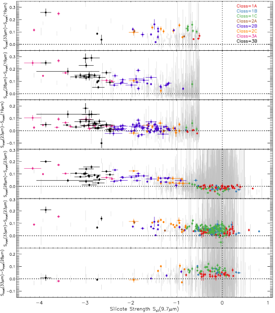
Figure 21: Strength differences between the four crystalline silicate bands as a function of the 9.7 $\mu$m amorphous silicate strength. Sources shown as filled circles have detections of both crystalline bands. Sources shown as gray bars have limits on one or both crystalline bands. Since we fit the 19 $\mu$m crystalline band only at S${}_{\rm sil}<$-0.5, the strength differences in the upper panels are only defined at S${}_{\rm sil}<$-0.5.

Comparison of the strengths of the 19, 23, 28 and 33 $\mu$m crystalline silicate bands on a source-to-source basis provides another important insight: for every band pair the strength of the shorter wavelength feature is equal to or lower than that of the longer wavelength feature. This difference is largest for the most deeply obscured sources (S_sil$\sim$-4; class 3A) and gradually decreases as S_sil becomes less negative. Remarkably, this decrease appears to unfold in a similar way for galaxies on the mixing line towards classic AGNs (class 3A$\rightarrow$2A$\rightarrow$1A) and towards classic starburst galaxies (class 3A$\rightarrow$3B$\rightarrow$2B$\rightarrow$2C$\rightarrow$1C): look for the few orange colored class 2A sources mixed in with the turquoise and blue colored class 2B and 2C sources at intermediate silicate strength (S_sil=-2.4 to -0.8). The differences in band strengths are smallest for the galaxies at the other extreme of the silicate strength scale: for galaxies on the classic AGN-starburst mixing line (1A–1B–1C) for which the 9.8 $\mu$m silicate strength is close to zero and for which the 23, 28 and 33 $\mu$m crystalline silicate bands are observed to be mostly in emission (Fig. 20).

9.2 Silicate features in spectra of centrally heated dust geometries

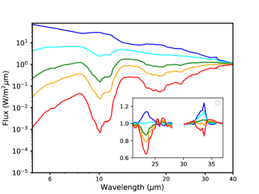
Figure 22: Simulated mid-infrared spectra of five centrally heated dust shells. The dust mass increases by a factor 100 from the top to the bottom spectrum (blue to red). Clearly visible at various wavelengths are the radiative transfer effects caused by enhanced opacity associated with the presence of amorphous and crystalline silicates at those wavelengths. The strongest of these opacity enhancements, centered at 9.8 and 18 $\mu$m, are associated with vibration modes of amorphous silicates. Narrower features, centered at 11, 16, 19, 23, 28 and 33 $\mu$m are vibration modes of crystalline silicates (forsterite). At the lowest dust column (blue spectrum), all silicate features are in emission, as the optical depth does not surpass unity at any wavelength. As the dust column increases, features switch from emission to absorption at wavelengths where the local optical depth exceeds unity. The highest optical depth is measured in the red spectrum: $\tau_{9.8}$=85. The inset shows the continuum-normalized spectral profiles of the 23 and 33 $\mu$m Forsterite features. The 23 $\mu$m band switches from emission to absorption at a lower dust column density than required for the 33 $\mu$m band to become optically thick.

The above observations are consistent with an origin for the amorphous and crystalline silicate features in a centrally heated dust geometry, either spherical in nature or arranged in a torus geometry.

In Fig. 22 we show simulated 5–40 $\mu$m spectra for five centrally heated dust shells with dust masses increasing by a factor 100 from the top to the bottom spectrum. The model spectra have been computed using the 2D version of the MCMAX code (Min et al., 2009), with the following parameters. For the central heating source we adopt a 2500 K stellar SED. The gas density falls off as r^-1, and is parametrized as in Meixner et al. (2002). The dust mixture is composed of 75% MgFeSiO₄ amorphous dust (Jena database optical constants; Dorschner et al. (1995)), 20% am-Carbon (optical constants of Zubko et al. (1996)), and 5% forsterite Mg₂SiO₄ (optical constants of Suto et al. (2006)). The optical constants are temperature dependent between 50 and 295 K. We adopt a dust size of 0.1 $\mu$m and a DHS grain shape distribution (Min et al., 2005) with f_max=0.8. As can be seen in Fig. 22, any departure from a flat or monotonously changing opacity curve as a function of wavelength will result in spectral structure to appear in the emerging spectrum of the centrally heated dust structure. For the model spectra in Fig. 22, the inclusion of minerals in the dust composition has the effect of increasing the dust opacity around the central wavelengths of the vibration modes of the included amorphous and crystalline silicate species. Radiative transfer then dictates that, if the dust structure is optically thin at all mid-infrared wavelengths, all mineral features will appear as emission features in the emerging spectrum (the dark blue spectrum in Fig. 22). Increasing the amount of dust around the heating source will result in the wavelength range to which the 9.8 $\mu$m mode of amorphous silicate contributes to become optically thick first, resulting in the feature to switch from an emission to an absorption feature (the light blue spectrum in Fig. 22) thanks to the negative temperature gradient in the centrally heated dust structure. Residing deep within the 9.8 $\mu$m amorphous silicate opacity profile, also the 11 $\mu$m forsterite band will be in the optically thick regime and, consequently, appear in absorption too. A further increase in the amount of dust around the heating source will bring the broad 18.5 $\mu$m amorphous silicate band, along with the narrower 16 and 19 $\mu$m crystalline silicate bands, into absorption as the optical depth at these wavelengths surpasses unity (the green and orange spectra in Fig. 22). Next are the 23 and 28 $\mu$m crystalline silicate bands. The last mid-infrared feature to go into absorption is the 33 $\mu$m crystalline silicate band. This is shown by the red spectrum in Fig. 22.

In the absence of PAH emission, the shortest wavelength silicate bands will be the most sensitive probes of the obscuring dust column. In practice, however, only above 20 $\mu$m PAH emission associated with circumnuclear star formation will not fill in the silicate emission and absorption features. This thus leaves the 23, 28 and 33 $\mu$m forsterite bands as the only suitable probes of nuclear obscuration in galaxy-integrated spectra.

Fig. 22 also clearly illustrates another radiative transfer effect: the redistribution of infrared radiation to longer wavelengths as the dust column increases. From the top to the bottom model SED the C(30 $\mu$m)/C(5.5 $\mu$m) continuum slope changes by several orders of magnitude. Unfortunately, stellar photospheric emission and PAH emission at 5.5 $\mu$m may contaminate the accuracy of this diagnostic by boosting the emission at 5.5 $\mu$m.

9.3 Tracers of nuclear obscuration in dusty galactic nuclei

Assuming the nuclei of dusty IDEOS sources to ressemble centrally heated dust geometries, we can use the 23 $\mu$m and 33 $\mu$m forsterite bands to devise a crude measure of nuclear obscuration:

• 23 $\mu$m and 33 $\mu$m bands in emission: low obscuration.

• 23 $\mu$m band in absorption and the 33 $\mu$m band in emission: intermediate obscuration.

• 23 $\mu$m and 33 $\mu$m bands in absorption: high obscuration.

These three regimes are illustrated in Fig. 23 by the 15–35 $\mu$m continuum-normalized spectra of three galaxies with decreasing silicate strengths (-0.13, -1.41, and -3.86). Note the absence of the 28 $\mu$m feature in the middle spectrum. In this source the dust continuum at 28 $\mu$m is likely in between optically thin and thick, rendering the feature undetectable despite a non-zero column of forsterite. This same effect can be seen among the model spectra in Fig. 22, where the 33 $\mu$m forsterite feature is indiscernible in the orange spectrum, which represents the second highest dust column density in the plot. Unfortunately, the proximity of the 33 $\mu$m forsterite band to the long wavelength spectral cut-off of IRS-LL1 limits the use of this diagnostic to sources at z$<$0.068. This thus excludes most of the local ULIRG population.

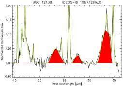
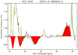
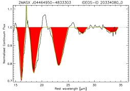
Figure 23: 16–33 $\mu$m crystalline silicate spectra arranged in order of increasing obscuration. Each spectrum is normalized by dividing the observed spectrum by the fitted continuum. In the top spectrum (S${}_{\rm sil}=$-0.13) all fitted crystalline bands (red) are in emission. In the bottom spectrum (S${}_{\rm sil}=$-3.86) all are in absorption. The spectrum in the middle panel (S${}_{\rm sil}=$-1.41) shows the 33 $\mu$m crystalline feature in emission and the 23 $\mu$m crystalline feature in absorption, while the feature in between, the 28 $\mu$m crystalline band, is undetected.

In our sample of 232 sources with detections for both the 23 and the 33 $\mu$m crystalline band we find no sources for which the 23 $\mu$m crystalline band is in emisson and the 33 $\mu$m feature is in absorption. Since this combination would be unphysical for a centrally heated dust structure, this means that, in principle, all these 232 sources could harbor a centrally heated dust structure.

Further insights can be gathered from overlaying our 23 and 33 $\mu$m crystalline silicate diagnostic onto the Fork Diagram (Sect. 8.1) and onto the diagram that delineates the slope of the 5.5–30 $\mu$m continuum and the 9.8 $\mu$m amorphous silicate strength (Sect. 8.2). As discussed in Sect. 8.1 & 8.2, these diagrams delineate three types of sources:

• Galaxies dominated by a centrally heated dust structure with low EQW(PAH62) and mostly cool mid-infrared colors (class 3A)

• Galaxies dominated by a classic AGN with similarly low EQW(PAH62) and warm mid-infrared colors (class 1A)

• Classic starburst galaxies with high EQW(PAH62) and cool mid-infrared colors (class 1C).

If we color-code galaxies with 23 $\mu$m & 33 $\mu$m bands that are both in emission as green, galaxies with the 23 $\mu$m band in absorption and the 33  $\mu$m band in emission as orange, and galaxies with the 23 $\mu$m & 33 $\mu$m bands both in absorption as blue, the upper panels of Fig. 24 show the blue (high obscuration) and green (low obscuration) galaxies to be clearly separated, with the orange (intermediate obscuration) sources found in between.

Since our sample of high-obscuration sources is quite small, we can use the sample’s S_cryst(23$\mu$m) and S_cryst(28$\mu$m) characteristics to find additional sources beyond the redshift cut-off for measuring the 33 $\mu$m forsterite band (z$>$0.068). Using the criterion S_cryst(23$\mu$m)$<$-0.09 and S_cryst(28$\mu$m)$<$-0.02 we find 32 additional high-obscuration galaxies up to z=0.257, which we plot along with the other high-obscuration sources as blue symbols in the lower panels of Fig. 24. This further populates the upper envelope of the diagonal branch in the Fork Diagram and the left half of the C(30 $\mu$m)/C(5.5 $\mu$m) versus silicate strength diagram, while still showing a clear separation between blue and green sources in both.

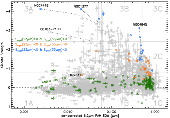
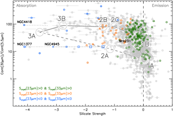
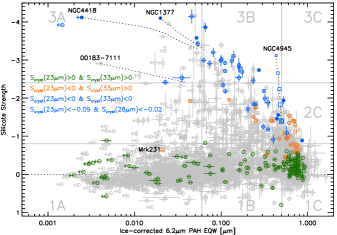
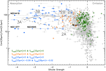
Figure 24: Left: Diagnostic diagram combining the ice-corrected equivalent width of the 6.2 $\mu$m PAH feature (Sect. 3.1) with the silicate strength. Sources plotted as gray circles are the same sources as in Fig. 14. Overplotted in color are sources with particular combinations of crystalline silicate strengths. Green denotes S_cryst(23 $\mu$m)$>$0 & S_cryst(33 $\mu$m)$>$0. Orange denotes S_cryst(23 $\mu$m)$<$0 & S_cryst(33 $\mu$m)$>$0. Blue filled circles denotes S_cryst(23 $\mu$m)$<$0 & S_cryst(33 $\mu$m)$<$0, whereas blue open circles denote S_cryst(23 $\mu$m)$<$-0.09 & S_cryst(28 $\mu$m)$<$-0.02. There are no occurences of S_cryst(23 $\mu$m)$>$0 & S_cryst(33 $\mu$m)$<$0. The dotted lines extending from NGC 4418, NGC 1377, and IRAS F00183–7111 in the direction of class 1C show the effect of adding circumnuclear star formation (NGC 4945 disk template) to the spectra of these sources. The lines end where the circumnuclear star formation reaches 20% of the total 5.5–13 $\mu$m flux. The connected blue squares show the effect of larger and larger spectral apertures centered on the nucleus of NGC 4945. Right: Diagnostic diagram of the rest frame 30 $\mu$m to 5.5 $\mu$m continuum ratio versus the 9.8 $\mu$m silicate strength. Sources and lines shown in gray are the same as in Fig. 15. Color-coding is the same as in the left panel.

For sources along the mixing line 3A$\rightarrow$2A$\rightarrow$1A, for which the obscuration decreases (silicate strength becomes less negative), this separation between high and low obscuration sources is more or less expected because emission components associated with star formation (e.g. PAH features) do not complicate the interpretation. For sources along the mixing line 3A$\rightarrow$3B$\rightarrow$2B$\rightarrow$2C$\rightarrow$1C (which traces the diagonal branch in the Fork Diagram), however, the observed separation between blue and green sources is less straightforward to interpret due to the increasing importance of exposed (as opposed to buried) star formation towards class 1C.

If circumnuclear star formation were negligible among the sources with crystalline silicate diagnostics in Fig. 24, the interpretation of the clear separation between blue and green sources and the presence of orange sources dotted in between would be straightforward: the nuclear power source becomes less and less buried along the mixing line from class 3A to class 1C. In a more realistic scenario, however, we recognize that the physical projected size covered by the Spitzer-IRS slit expands with redshift and will contain some or all of the galaxy disk in the majority of our spectra. The 23–33 $\mu$m crystalline signatures of the nuclear SED will thus be polluted with optically thin, warm dust continuum emission associated with circumnuclear star formation. Diaz-Santos et al. (2010) have shown that these contributions can be significant. For ULIRGs up to 30% of the 5–15 $\mu$m emission may originate from outside the nucleus (Marshall et al., 2018).

We have used the IRS mapping observations of the nearby Seyfert-2 galaxy NGC 4945 (Spoon et al. in prep.; Peréz-Beaupuits et al., 2011) to create a 5–36 $\mu$m template spectrum of cicumnuclear star formation. The spectrum comprises all spatial positions in a LL1-gridded map where S_sil$>$-0.6, thus excluding the deeply buried nucleus. While the nuclear spectrum clearly shows the 23 and 33 $\mu$m forsterite bands in absorption, the circumnuclear spectrum is devoid of crystalline silicate bands. If the absence of crystalline features in this galaxy disk spectrum is representative for galaxy disks in general , circumnuclear star formation will not change the diagnostic power of the 23 and 33 $\mu$m forsterite bands, as adding continuum to the nuclear SED will only weaken the nuclear crystalline features, but not flip them from emission to absorption, or vice versa. The main result will be a displacement of the source in the Fork Diagram towards class 1C as the silicate feature fills up and PAH emission features strengthen compared to the continuum. This effect is illustrated by the dotted tracks originating from the buried nuclei of NGC 4418, NGC 1377 (Roussel et al., 2006), and IRAS F00183–7111 (Spoon et al., 2004) in all panels of Fig. 24, and by the track for different sized apertures centered on the buried AGN in NGC 4945.

In this interpretation, the lone blue point among a sea of orange in the Fork Diagram, close to the border of quadrants 2C and 1C (at EQW(PAH62)=0.86 $\mu$m and S_sil=-0.88), has to be a galaxy with a deeply buried nucleus, which has been displaced in the direction of class 1C by a strong contribution of circumnuclear star formation. Indeed, archival HST imaging of IRAS 17578–0400N shows complex extended emission around the galaxy nucleus (Armus, priv. comm.). And HCN mm-observations by Falstad et al. (2021) result in the nucleus to be classified as a ’CON’, a compact obscured nucleus. Circumnuclear star formation is thus able to disguise a buried nucleus at wavelengths below 20 $\mu$m, but not above. The classification into blue, orange and green points thus seems to be a better indication for the level of dust obscuration in a nucleus than the position of a source in the Fork Diagram. Only if aperture sizes were chosen to exclude the galaxy disks the Fork Diagram diagnostic features and the crystalline diagnostics would likely be in agreement.

Since in the Fork Diagram there are no orange or green labeled sources identified below S_sil=-2, it may be reasonable to regard all galaxies below this limit as hosting a deeply obscured nucleus. This would increase the total count of confirmed deeply obscured nuclei from 40 to 89.

Also note the position of the intermediate dust enshrouded nucleus of Mrk 231 (color-coded orange) in the left panels of Fig. 24, close to the locus of the classical AGNs on the horizontal branch. Unlike Mrk 231, classical AGN do not show evidence for centrally heated dust geometries as revealed by their assigned green color-code. The simplest explanation for the proximity of Mrk 231 to the classical AGN is that the dust structure which covers the central power source has a small opening through which unattenuated continuum leaks out and fills up the 9.8 $\mu$m silicate absorption feature. As modeled by Marshall et al. (2018), such a “keyhole” can be fairly small: less than 10% of the surface area of the mid-infrared shell. The additional continuum does not affect the crystalline silicate diagnostics, as it cannot flip the 23 $\mu$m forsterite feature from absorption to emission as required to turn the source from orange to green in Fig. 24. The nucleus of Mrk 231 is thus more deeply obscured than the silicate strength indicates. Interestingly, this conclusion is supported by our spectral decomposition using QUESTFIT (Sect. 4.2), which requires one deeply obscured component and one unobscured component for the best fit. Further evidence in support of this conclusion will be presented below.

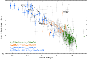
Figure 25: Ratio of the 12.7 $\mu$m to the 11.2 $\mu$m PAH feature as a function of silicate strength for sources with 8$\sigma$ detections of both features. Sources shown in blue, orange or green have detections for both the 23 and 33 $\mu$m crystalline silicate bands. Color-coding is the same as in Fig.24. Overlaid are two tracks showing the effect of increased galaxy disk contribution. The track with squares superimposed shows the effect of increasing the aperture size centered on the nucleus of NGC 4945 from 13$"$$\times$13$"$ to 76$"$$\times$31.5$"$. The other track (diamonds) shows the effect of adding disk emission (using the NGC 4945 disk template) to the spectrum of NGC 4418. The percentages listed alongside the latter track indicate the circumnuclear contribution as part of the total 5.5–13 $\mu$m emission for that track.

Another probe of the obscuration in a galactic nucleus is the ratio of the 12.7 and 11.2 $\mu$m PAH fluxes. This ratio is sensitive to the silicate column density through the effects of differential extinction in the steep red wing of the 9.8 $\mu$m silicate feature. This aspect was explored by Hernán-Caballero et al. (2020) using a subsample of IDEOS sources. In the absence of obscuration the PAH127/PAH112 ratio has a median value of 0.38 with a 5% dispersion (related to PAH excitation conditions in individual galaxies). As shown in Fig. 25, the PAH112 feature weakens relative to the PAH127 feature as the silicate strength becomes more negative. The highest observed PAH127/PAH112 ratio in our sample, and the highest permitted ratio in CHUNKFIT (Sect. 3.3), occurs among the most deeply buried sources: PAH127/PAH112=1.3. While the large majority of galaxies scatters around the diagonal line in the plot, there are some clear outliers: galaxies for which the silicate strength is less negative than based on just the PAH ratio. For some of these galaxies, mostly classic AGN, the high ratio reflects intrinsic conditions in the galaxy, while in other cases the PAH112 and PAH127 features were observed in different spectral orders (e.g. SL1 and LL2), which may result in spectral stitching-related fitting anomalies. Colored data points in Fig. 25 are sources for which our 23 & 33 $\mu$m and 23 & 28 $\mu$m crystalline silicate diagnostics are available. Again we see a clear separation between the sources color-coded in blue and green, with intermediate obscuration nuclei (color-coded in orange) found in between. This distribution suggests that the silicate strength, the crystalline silicate diagnostics, and the PAH127/PAH112 ratio largely trace each other.

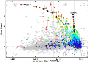
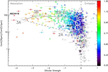
Figure 26: Left: Diagnostic diagram combining the ice-corrected equivalent width of the 6.2 $\mu$m PAH feature (Sect. 3.1) with the silicate strength. The sources plotted in gray are the same sources as in Fig. 14. Overplotted in rainbow colors (see legend in right panel) are sources with detections of both the PAH11 and the PAH127 feature. Red denotes a PAH127/PAH11 ratio around 1.3, while black denotes a PAH127/PAH11 ratio below 0.25. Overplotted are two tracks. The track for NGC 4945 shows how the PAH127/PAH11 ratio changes as the aperture centered on the nucleus increases in size from 5.5$"$$\times$5.5$"$ to 76$"$$\times$31.5$"$. The other track shows how the PAH127/PAH11 ratio changes when more and more disk emission (NGC4945 template) is added to the spectrum of NGC 4418. The percentage listed indicates what fraction of the total 5.5–13 $\mu$m flux is comprised of disk emission. Right: Diagnostic diagram of the rest frame 30 $\mu$m to 5.5 $\mu$m continuum ratio versus the 9.8 $\mu$m silicate strength. Sources and lines shown in gray are the same as in Fig. 15. The color-coding is the same for both panels.

Overlaid on the plot are two tracks. The first one, connecting the four dark squares, show where the spectra of different sized apertures (13$"$$\times$13$"$ to 76$"$$\times$31$"$) centered on the buried nucleus of NGC 4945 fall on the plot. The other track shows the effect of adding circumnuclear star formation (using the NGC 4945 circumnuclear template) to the spectrum of NGC 4418. Both tracks clearly show that, as more circumnuclear star formation is added to the spectrum of a buried source, the source shift towards a lower PAH ratio and a less negative silicate strength without leaving the distribution. The PAH127/PAH112 ratio by itself is thus not a good tracer of nuclear obscuration unless the spectral slit is small enough to isolate the nucleus. The ability of sources to shift to the lower right along the diagonal may explain the presence of several blue sources among the orange ones. For instance IRAS 17578–0400N at S_sil=-0.88 and PAH127/PAH112=0.51, discussed before.

The figure also shows Mrk 231 to be located far to the right of the main correlation. For the observed PAH127/PAH112 ratio of 0.93 to fit in with the main trend, the silicate strength would have to be much more negative: -2 to -2.5 rather than -0.63. As discussed above, unobscured mid-infrared emission protruding from a key hole opening in the obscuring shell may fill in the silicate feature and cause Mrk 231 to shift to the right.

Fig. 26 shows the Fork Diagram and the 30-to-5.5 $\mu$m versus silicate strength diagram color-coded by the value of the PAH127/PAH112 ratio. Along the class 3A$\rightarrow$3B$\rightarrow$2B$\rightarrow$2C$\rightarrow$1C mixing line the PAH ratio shows a clear progression towards a lower ratio. When interpreted as an extinction probe, this suggests a decrease of nuclear obscuration from class 3A to class 1C. Overlaid on the Fork Diagram are two tracks showing the effect on the PAH ratio of adding circumnuclear star formation. One track for NGC 4945, using aperture sizes increasing from 5.5$"$$\times$5.5$"$ to 76$"$$\times$31.5$"$ centered on the buried nucleus, the other showing the effect of adding circumnuclear star formation to the deeply obscured nucleus of NGC 4418. As can be clearly seen, the color-coding of the tracks blends in perfectly with the galaxy-integrated observations underneath. This confirms that the presence of circumnuclear star formation affects the PAH ratio in the same way as a decrease of nuclear obscuration does. Thus, unlike the crystalline silicate diagnostic, the PAH127/PAH112 ratio by itself cannot produce conclusive evidence for a decrease of nuclear obscuration from class 3A towards class 1C. It may at best be supportive.

9.4 The crystallinity of the ISM in dusty galactic nuclei

More than a decade ago, Spoon et al. (2006) used the strengths of the 16 $\mu$m crystalline silicate feature and 9.7 $\mu$m amorphous silicate feature to infer the crystallinity of the ISM in a sample of ULIRGs. The method assumes that the feature arises from a column of cold dust in front of a warm central source. Under these conditions the radiative transfer equation lacks an emission term. Here we prefer to use the 19 $\mu$m crystalline band instead, because it is more frequently detected and modeled in Galactic sources (see Appendix C). Following Kemper et al. (2004) we define the crystallinity of the ISM as

$$C_{\rm ISM}=\frac{N_{\rm cryst}}{N_{\rm cryst}+N_{\rm am}}$$ (10)

where N_cryst and N_am are the column densities of crystalline and amorphous silicates, respectively. For sources with amorphous silicates firmly in absorption (S${}_{\rm sil}<$-1), this becomes

$$C_{\rm ISM}(19\mu m)=\frac{S_{\rm cryst}(19\mu m)/\kappa_{\rm cryst}(19\mu m)}{S_{\rm cryst}(19\mu m)/\kappa_{\rm cryst}(19\mu m)+S_{\rm sil}/\kappa_{\rm am}(9.7\mu m)}$$ (11)

where $\kappa_{\rm am}$(9.7$\mu$m) is the peak mass absorption coefficients of amorphous silicates at 9.7$\mu$m, 2.4$\times$10³ cm² g^-1 (Dorschner et al., 1995), and $\kappa_{\rm cryst}$(19$\mu$m) is the baseline-subtracted peak mass absorption coefficients of Forsterite at 19$\mu$m, 4.8$\times$10³ cm² g^-1. The latter was computed with the grain model of Min et al. (2005), using the optical constants of Suto et al. (2006) for Forsterite at T=200K, and adopting a distribution of hollow spherical grains with 0.1 $\mu$m radius and a maximum vacuum fraction of 80%. As can be seen in Fig. 27, this results in 19$\mu$m-crystallinities between 0.7% and 6% for obscured nuclei (S_sil$<$-1) with a detection of the 19$\mu$m crystalline silicate absorption feature (114/254 sources), and in upper limits as low as 0.3% for sources with a non-detection of the feature (140/254 sources). On average the 19$\mu$m crystallinity of these obscured nuclei (S_sil$<$-1) is 2.7%, with both the most uncertain crystallinities and the strictest upper limits occurring among the least obscured sources.

The large spread in crystallinities seen in Fig. 27 may very well explain why among sources with deep silicate absorption features (S_sil$<$-2) and non-zero crystallinities we see so many non-detections of 28 and 33$\mu$m crystalline bands in Fig. 20. Examples are IRAS 02530+0211 (S_sil=-3.6; C_ISM(19$\mu$m)=1.2%) and IRAS 00188–0856 (S_sil=-2.7; C_ISM(19$\mu$m)=0.8%), which have 3–4 times lower crystallinities than for instance IRAS 04454–4838 (S_sil=-3.9; C_ISM(19$\mu$m)=3.6%).

Finally, are there any galaxies at S_sil$<$-1 that lack detectable crystalline silicates to strict limits? To investigate this question we have five crystalline silicate bands at our disposal. We consider a band undetected if S_cryst(19$\mu$m)$>$-0.016, $|$S_cryst(23$\mu$m)$|<$0.010, $|$S_cryst(28$\mu$m)$|<$0.015, or $|$S_cryst(33$\mu$m)$|<$0.02. Among the 70 sources at S_sil$<$-1 with coverage of all five cystalline silicate bands we find none that meets the strict upper limits set for a non-detection of all five bands.

9.5 The detection rate of crystalline silicates in other galaxies

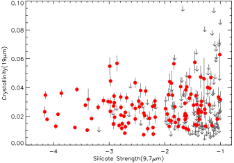
Figure 27: Crystallinity of the interstellar medium in galaxies with measurements of the 9.7 $\mu$m amorphous silicate absorption feature and the 18.5 $\mu$m crystalline silicate absorption feature. Upper limits are shown as gray arrows.

For the 2526 galaxies in our sampe that are not (deeply) enshrouded (S_sil$>$-1) our method is not suitable to infer a crystallinity as the features it relies on are not optically thick. We can determine, though, whether in a spectrum crystalline silicates are present or absent to meaningful limits by taking stock of the measured crystalline silicate strengths in the 23, 28 and 33 $\mu$m bands. While we won’t be able to infer a column density without generating a full radiative transfer model for these galaxies, this exercise may provide insight into the prevalence of crystalline silicates and the conditions under which they can survive.

Apart from galaxies with detections of one, two, or all three bands, there are only four galaxies among 874 galaxies at S_sil$>$-1 with coverage of all three bands and the high S/N in their 22–34 $\mu$m spectra required to get below these strict limits that do not show any evidence for the presence of these bands. These galaxies are 2MASS J19563578+1119050 (S_sil=-0.97), ESO 239-IG002 (S_sil=-0.42), II Zw 40 (S_sil=-0.34), and 3C 390.3 (S_sil=+0.09). All are marked by black error bars in Fig. 20. For three of these, their silicate strength in the -0.3 to -1.0 range may imply that the 23, 28 and 33 $\mu$m bands are simply not fully sensitive to what would be a detectable column density at a different silicate strength. This leaves 3C 390.3 as the only source for which the strict non-detection of crystalline silicate bands may be significant. That is, if synchrotron emission at 33 $\mu$m can be ruled out as a source of dilution of the 33 $\mu$m forsterite band of this broad-line radio galaxy.

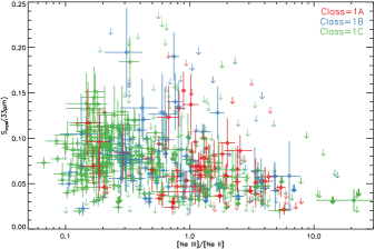
Figure 28: Strength of the 33 $\mu$m crystalline silicate emission band as a function of the hardness of the radiation field in galaxies at S_sil$>$-0.8. Thick upper limit symbols denote the detection of the 23 $\mu$m forsterite band either in emission or absorption.

Is there more that we can learn from the detectability of crystalline silicate features in sources at S_sil$>$-1 ? All 2120 galaxies on the horizontal branch of the Fork Diagram (Fig. 14; classes 1A/B/C; S_sil$>$-0.8) have one thing in common: the 33 $\mu$m crystalline silicate band is expected to be seen in emission (see Fig. 20). Whether the band is discernable is not just a matter of column density or temperature of the crystalline silicates, though, but also depends on the strength of the local 33 $\mu$m continuum and the strengths of the 33.48 $\mu$m [S iii] and 34.82 $\mu$m [Si ii] emission lines. With these caveats in mind, we looked for trends among the 834 class 1A/B/C sources at redshifts below z=0.068 for which the 33 $\mu$m crystalline silicate band was in range.

Fig. 28 shows the 33 $\mu$m crystalline silicate strength as a function of the hardness of the radiation field as measured by the [Ne iii]/[Ne ii] ratio. As can be clearly seen, the upper envelope of S_cryst(33$\mu$m) decreases towards a higher neon ratio with no distinction between mid-infrared galaxy class (as shown by color coding). Above [Ne iii]/[Ne ii]=6.5 there is only one more galaxy with a detection of the 33$\mu$m forsterite band: the low-metallicity galaxy SHOC 391 at [Ne iii]/[Ne ii]=22. This is, however, not the only galaxy above [Ne iii]/[Ne ii]=6.5 with a detection of forsterite. As shown by thick upper limit symbols, there are two sources with detections of the 23$\mu$m forsterite band, in absorption: the low-metallicity galaxies SBS 1533+574B and IRAS 11485–2018. A similar trend can be seen by using [O iv]/[Ne ii] or [O iv]/[S iii] 33 $\mu$m instead, with one important difference: since all low-metallicity galaxies have upper limits for the [O iv] line, as is true for all galaxies powered by stellar sources of ionizing radiation (see e.g. Fig. 18), these galaxies appear along with other star forming galaxies towards the extreme left in those diagrams.

Since a silicate strength is measured relative to the local continuum, it is possible that the observed decrease in S_cryst(33$\mu$m) with increasing [Ne iii]/[Ne ii] can be fully attributed to an increase in the 33 $\mu$m flux density. The comparison of the panchromatic SED modeling of Galliano et al. (2008a) to the mid-IR spectral decomposition of Galliano et al. (2008b), for 30 nearby galaxies, indeed shows that an increase in [Ne iii]/[Ne ii] is accompanied by an increase in 33 $\mu$m dust emission relative to the total IR emission. Since it is beyond the scope of the current paper to include far-infrared data, we cannot determine whether the crystallinity decreases as the hardness of the ionizing SED increases, or whether the 33 $\mu$m crystalline silicate feature gets overwhelmed by the 33 $\mu$m dust continuum.

Attempts to find correlations of S_cryst(33$\mu$m) with the 30 $\mu$m to 5.5 $\mu$m continuum slope and with EQW(PAH62) have come up empty. In the absence of a mid-infrared diagnostic that allows us to distinguish between quiescent and vigorous star formation among IDEOS galaxies we also cannot address the question whether the higher input of stardust in a galaxy would have a measurable effect on the global dust content.

For the IDEOS sample as a whole it thus appears that crystalline silicates are a common component of the ISM of galaxies — or, taking into account the non-detection of crystalline silicates in the spectra of the disks of NGC 4945 and M 101 (Sect. 9.3), of galactic nuclei.

10 IDEOS portal

The results of our spectral fitting and decomposition can be examined in detail via the IDEOS web portal ideos.astro.cornell.edu. The website offers several important functionalities beyond what machine-readable tables of measured quantities offer, such as, for individual sources:

• The extraction positions and positions angles for the individual SL and LL nod spectra are overlaid on an optical survey map.

• The nod1 and nod2 spectra are plotted together to allow assessment of the significance of spectral structure found in the final nod-averaged spectrum.

• Continuum, line and feature fits can be visually inspected by choosing the SED fit of the appropriate wavelength range.

• Amorphous and crystalline silicate band fits are plotted side-by-side.

• All fitted emission lines can be compared in one plot.

• The excitation diagram of warm molecular hydrogen, and postage stamp plots of the individual H₂ line fits are shown together.

• Synthetic photometric points are overlaid on the SED.

• The spectral decomposition into PAH and blackbody components from either PAHFIT or QUESTFIT is visualized.

The portal also provides a way to rank and examine sources by any of the measured quantities, or to select a galaxy sample based on constraints built on inequalities of observables conjoined by logical operators. E.g. irs15flux $>$ 2 $*$ mips24flux, ne3_15flux $>$ ne2flux, or redshift $>$ 0.3. The observables and spectra can also be downloaded as machine readable tables.

Within the portal we also link to auxilary pages that explain the characteristics of CHUNKFIT or how we came to adopt our spectral resolution table.

Table 6: IDEOS observables: emission and absorption features

Column	Observable	Unit	Description
1	Name		IDEOS identifier
2	Galaxy		NED galaxy identifier
3	RA	degrees	Right Ascension J2000.0
4	Dec	degrees	Declination J2000.0
5	z		Redshift (Paper i)
6	MirClass		Mid-IR class designation
7–9	Pah62Flux	W m-2	6.2 $\mu$m PAH flux measured using spline method
10–12	Pah62EQW	$\mu$m	Ice-corrected equivalent width of the 6.2 $\mu$m PAH feature measured using spline method
13–15	Pah11Flux	W m-2	11.2 $\mu$m PAH flux (sum of PAH111 and PAH112) measured using spline method
16–18	Pah11EQW	$\mu$m	Equivalent width of the 11.2 $\mu$m PAH feature measured using spline method
19–21	Pah127Flux	W m-2	12.7 $\mu$m PAH flux measured using spline method
22–24	Pah127EQW	$\mu$m	Equivalent width of the 12.7 $\mu$m PAH feature measured using spline method
25–27	DrudePAH62FLUX	W m-2	6.2 $\mu$m PAH flux measured using drude method
28–30	DrudePAH62EQW	$\mu$m	Ice-corrected equivalent width of the 6.2 $\mu$m PAH feature measured using drude method
31–33	DrudePAH77Flux	W m-2	7.7 $\mu$m PAH flux measured using drude method
34–36	DrudePAH77EQW	$\mu$m	Equivalent width of the 7.7 $\mu$m PAH feature measured using drude method
37–39	DrudePAH11Flux	W m-2	11.2 $\mu$m PAH flux measured using drude method
40–42	DrudePAH11EQW	$\mu$m	Euivalent width of the 11.2 $\mu$m PAH feature measured using drude method
43–45	DrudeTOTPahFlux	W m-2	Integrated flux of all 5–19 $\mu$m PAH feature measured using drude method
46–48	DrudeMirFlux	W m-2	Integrated 5–25 $\mu$m continuum flux using drude method
49	DrudeOrigin		Decomposition method: PAHFIT or QUESTFIT
50–52	SilStrength		Strength of the 9.8 $\mu$m amorphous silicate feature
53	SilFitType		Interpolation method used to create local continuum: powerlaw or spline
54	SilAnchorType		Origin of anchors for continuum interpolation
55–57	Cryst19Strength		Strength of the 19 $\mu$m crystalline silicate feature
58–60	Cryst23Strength		Strength of the 23 $\mu$m crystalline silicate feature
61–63	Cryst28Strength		Strength of the 28 $\mu$m crystalline silicate feature
64–66	Cryst33Strength		Strength of the 33 $\mu$m crystalline silicate feature
67–68	TauIce		Optical depth of the 6 $\mu$m ice feature
69–70	Tau685		Optical depth of the 6.85 $\mu$m aliphatic feature

Table 7: IDEOS observables: emission lines

Column	Observable	Unit	Description
71–73	Ar2Flux	W m-2	6.99 $\mu$m [Ar ii] line flux
74–76	Ar3Flux	W m-2	8.99 $\mu$m [Ar iii] line flux
77–79	Cl2Flux	W m-2	14.37 $\mu$m [Cl ii] line flux
80–82	Fe2Flux	W m-2	25.99 $\mu$m [Fe ii] line flux
83–85	H2S0Flux	W m-2	28.22 $\mu$m H2 0–0 S(0) line
86–88	H2S1Flux	W m-2	17.03 $\mu$m H2 0–0 S(1) line
89–91	H2S2Flux	W m-2	12.28 $\mu$m H2 0–0 S(2) line
92–94	H2S3Flux	W m-2	9.66 $\mu$m H2 0–0 S(3) line
95–97	H2S5Flux	W m-2	6.91 $\mu$m H2 0–0 S(5) line
98–100	H2S7Flux	W m-2	5.51 $\mu$m H2 0–0 S(7) line
101-103	Ne2Flux	W m-2	12.81 $\mu$m [Ne ii] line flux
104–106	Ne3_15Flux	W m-2	15.56 $\mu$m [Ne iii] line flux
107–109	Ne3_36Flux	W m-2	36.01 $\mu$m [Ne iii] line flux
110–112	Ne5_14Flux	W m-2	14.32 $\mu$m [Ne v] line flux
113–115	Ne5_24Flux	W m-2	24.32 $\mu$m [Ne v] line flux
116–118	O4Flux	W m-2	25.89 $\mu$m [O iv] line flux
119–121	S3_18Flux	W m-2	18.71 $\mu$m [S iii] line flux
122–124	S3_33Flux	W m-2	33.48 $\mu$m [S iii] line flux
125–127	S4Flux	W m-2	10.51 $\mu$m [S iv] line flux
128–130	Si2_Flux	W m-2	34.82 $\mu$m [Si ii] line flux
131–133	Ar3Ar2Ratio		8.99 $\mu$m [Ar iii] / 6.99 $\mu$m [Ar ii]
134–136	Ne3_15Ne2Ratio		15.56 $\mu$m [Ne iii] / 12.81 $\mu$m [Ne ii]
137–139	Ne5_14Ne2Ratio		14.32 $\mu$m [Ne v] / 12.81 $\mu$m [Ne ii]
140–142	Ne5_24Ne2Ratio		24.32 $\mu$m [Ne v] / 12.81 $\mu$m [Ne ii]
143–145	O4Ne2Ratio		25.89 $\mu$m [O iv] / 12.81 $\mu$m [Ne ii]
146–148	O4S3_33Ratio		25.89 $\mu$m [O iv] / 33.48 $\mu$m [S iii]
149–151	O4S3_18Ratio		25.89 $\mu$m [O iv] / 18.71 $\mu$m [S iii]
152–154	S3_33S3_18Ratio		33.48 $\mu$m [S iii] / 18.71 $\mu$m [S iii]
155–157	S4S3_18Ratio		10.51 $\mu$m [S iv] / 18.71 $\mu$m [S iii]
158–160	Si2S3_33Ratio		34.82 $\mu$m [Si ii] / 33.48 $\mu$m [S iii]

Table 8: IDEOS observables: synthetic photometry and rest frame continuum flux densities

Column	Observable	Unit	Description
161–162	IRAC8Flux	mJy	Synthetic IRAC 8 $\mu$m photometry
163–164	IRS15Flux	mJy	IRS blue peak-up photometry
165–166	IRS22Flux	mJy	IRS red peak-up photometry
167–168	MIPS24Flux	mJy	MIPS 24 $\mu$m photometry
169–170	MIRI56Flux	mJy	Synthetic MIRI 5.6 $\mu$m photometry
171–172	MIRI77Flux	mJy	Synthetic MIRI 7.7 $\mu$m photometry
173–174	MIRI10Flux	mJy	Synthetic MIRI 10 $\mu$m photometry
175–176	MIRI11Flux	mJy	Synthetic MIRI 11.3 $\mu$m photometry
177–178	MIRI13Flux	mJy	Synthetic MIRI 12.8 $\mu$m photometry
179–180	MIRI15Flux	mJy	Synthetic MIRI 15 $\mu$m photometry
181–182	MIRI18Flux	mJy	Synthetic MIRI 18 $\mu$m photometry
183–184	MIRI21Flux	mJy	Synthetic MIRI 21 $\mu$m photometry
185–186	MIRI25Flux	mJy	Synthetic MIRI 25.5 $\mu$m photometry
187–188	WISE12Flux	mJy	WISE band 3 photometry
189–190	WISE22Flux	mJy	WISE band 4 photometry
191–193	CONT37Flux	mJy	Rest frame continuum flux density at 3.7 $\mu$m
194–196	CONT42Flux	mJy	Rest frame continuum flux density at 4.2 $\mu$m
197–199	CONT55Flux	mJy	Rest frame continuum flux density at 5.5 $\mu$m
200–202	CONT97Flux	mJy	Rest frame continuum flux density at 9.7 $\mu$m
203–205	CONT15Flux	mJy	Rest frame continuum flux density at 15 $\mu$m
206–208	CONT24Flux	mJy	Rest frame continuum flux density at 24 $\mu$m
209–211	CONT30Flux	mJy	Rest frame continuum flux density at 30 $\mu$m
212–214	C15C55Ratio		Rest frame continuum slope 15 $\mu$m/5.5 $\mu$m
215–217	C24C55Ratio		Rest frame continuum slope 24 $\mu$m/5.5 $\mu$m
218–220	C30C55Ratio		Rest frame continuum slope 30 $\mu$m/5.5 $\mu$m
221	SNR66		Continuum S/N at 6.6 $\mu$m
222	SNR9		Continuum S/N at 9.0 $\mu$m
223	SNR1125		Continuum S/N at 11.25 $\mu$m
224	SNR1325		Continuum S/N at 13.25 $\mu$m
225	SNR14		Continuum S/N at 14 $\mu$m
226	SNR17		Continuum S/N at 17 $\mu$m
227	SNR24		Continuum S/N at 24 $\mu$m
228	SNR30		Continuum S/N at 30 $\mu$m
229	SL2ScalingFactor		Factor by which the SL2 spectral segment has been scaled
230	SL1ScalingFactor		Factor by which the SL1 spectral segment has been scaled
231	LL2ScalingFactor		Factor by which the LL2 spectral segment has been scaled
232	LL1ScalingFactor		Factor by which the LL1 spectral segment has been scaled

11 Discussion

An unexpected by-product of the spectral fitting of the IDEOS spectra has been the discovery of crystalline silicate emission and absorption features in the 23–34 $\mu$m range of almost all good S/N spectra with coverage of these features. The large majority of these spectra show these forsterite features in emission: 417 times in emission and 9 times in absorption for the 33 $\mu$m feature; 97 times in emission and 76 times in absorption for the 28 $\mu$m feature; 320 times in emission and 235 times in absorption for the 23 $\mu$m feature. Only the shorter wavelength 16 and 19 $\mu$m forsterite features are fitted exclusively in absorption in spectra that satisfy S_sil$<$-0.5, where they are detected 149 times.

We have found that the strength of the five fitted crystalline features is correlated with the strength of the 9.8 $\mu$m amorphous silicate feature (Fig. 20) and that the longer wavelength crystalline silicate bands require a deeper 9.8 $\mu$m silicate absorption feature for them to be seen in absorption than their shorter wavelength counterparts (Figs. 22 & 23). These findings are reminiscent of the structure seen in spectra of evolving AGB stars. The silicate bands in these sources are found to be in emission or absorption (see Fig. 33) depending on the thickness of the dust shell (Sylvester et al., 1999; Dijkstra et al., 2003; de Vries et al., 2014; Golriz et al., 2014).

For galaxies in our sample for which all silicate features are seen in emission (105 sources) in theory another kind of dust geometry may apply: that of a class i or ii protoplanetary disc (Meeus et al., 2001; Watson et al., 2009; Furlan et al., 2011). In these flared discs the dust temperature increases away from the mid-plane, as the surface layer of the disc is directly exposed to the radiation of the protostar. As a result all silicate features are seen in emission. Most of the IDEOS sources that share these spectral properties are AGN, whose dust geometries may have many similarities to those of protoplanetary disks.

In analogy to the evolving AGB stars discussed above, IDEOS galaxies with at least one forsterite band in absorption (323 sources) should host a centrally heated dust structure, which we identify with the galaxy’s nucleus. As illustrated in Fig. 22, the 23 and 33 $\mu$m forsterite bands can be used to classify galaxies as hosting a deeply obscured, semi obscured and unobscured nucleus. With the 28 $\mu$m forsterite feature as a proxy for the 33 $\mu$m forsterite feature in sources for which the 33 $\mu$m forsterite band is redshifted out of the IRS wavelength range, we are able to identify a total of 40 deeply obscured galactic nuclei. As can be seen in Fig. 24, not all of these sources (color-coded as blue) are found in the upper left part of the Fork Diagram (class 3A), which is home to the most deeply obscured galactic nuclei. As demonstrated in Sect. 9.3, circumnuclear star formation shifts these sources along the diagonal branch of the Fork Diagram towards class 1C. Class 3A is hence the locus of ’naked’ buried nuclei: those that are not ’dressed up’ with circumnuclear star formation. We predict that millimetre HCN-vib studies looking for Compact Obscured Nuclei (CONs; Falstad et al., 2021) will expose most of our 40 deeply obscured galaxies as CONs. We are especially confident about this since all CONs and non-CONs in the sample of Falstad et al. (2021) align with our crystalline silicate-based classifications for the sources that we have in common.

The case of Mrk 231 offers another lesson. Our crystalline diagnostics classify this ULIRG as containing a semi-obscured nucleus (the 33 $\mu$m feature is in emission, the 23 $\mu$m feature in absorption). A keyhole view through the obscuring dust shell (Marshall et al., 2018) of this BAL QSO results in a significant reduction of the depth of the 9.8 $\mu$m silicate feature, resulting in a significant downward shift in the Fork Diagram. The silicate strength is hence not a good proxy for the level of nuclear obscuration if: 1. There are light leaks (e.g. Mrk 231). 2. Circumnuclear star formation strongly contributes to the integrated SED (e.g. NGC 4945). 3. The dust distribution is clumpy (Nenkova et al., 2002). Sources well below the diagonal branch of the Fork Diagram may thus be affected by these AGN orientation effects or by light leaks.

For sources with a centrally heated dust geometry one can attempt to infer the crystallinity of the ISM, provided that both the amorphous and the crystalline silicate band used to probe the column density are in the optically thick regime. The shorter the wavelengths of the features used, the more easily this precondition is met. Kemper et al. (2004) exploited the proximity of the 11.2 $\mu$m forsterite band to the 9.8 $\mu$m amorphous silicate band to infer an upper limit of C_ISM(11.2 $\mu$m)=0.011 to the crystallinity of the Galactic Center line of sight. Contamination by 11.2 $\mu$m PAH emission forced Spoon et al. (2006) to use a longer wavelength forsterite band, at 16.3 $\mu$m, for their crystallinity determinations in a sample of 12 ULIRGs. They found C_ISM(16 $\mu$m) to range from 0.07 to 0.13. For the centrally heated sources in the IDEOS sample we have used the more commonly studied 19 $\mu$m forsterite band and were able to infer crystallinities for 254 sources. We found an average crystallinity C_ISM(19 $\mu$m)=0.027 with no apparent dependence on the silicate strength (see Fig. 27). These crystallinities are far lower than previously reported by Spoon et al. (2006) for their ULIRG sample and can be entirely explained by our different assumption for the mass absorption coefficient and our different choice of forsterite band for the measurement (see Appendix C). X-ray absorption spectroscopy probing the dense ISM towards bright X-ray binaries in the Galactic Center region (Rogantini et al., 2020; Zeegers et al., 2019) has revealed average crystallinities to be markedly higher (on the order of 10%) than the upper limit (1.1%) derived from the non-detection of the 11.2 $\mu$m forsterite band Kemper et al. (2004) towards Sgr A^∗. Our IR-derived crystallinities may thus be equally underestimating the true forsterite abundance in galactic nuclei.

An intriguing result of our study is that it appears that crystalline silicate features are present in all galaxy spectra obtained at sufficient S/N. Depending on the dust configuration and the S/N at 16–34 $\mu$m the detections may be limited to just the strong 33 $\mu$m forsterite feature in emission, a 23 $\mu$m feature in absorption, or a bucket-shaped 18 $\mu$m silicate absorption feature carved out by forsterite absorption at 16 and 19 $\mu$m. Fact is that our analysis shows that only one source, 3C 390.3, positively shows no crystalline silicate bands to the strict limits we set for non-detection of the forsterite bands. Even though we cannot exclude the existence of more sources like 3C 390.3 hiding among lower S/N spectra in our sample, the results found based on 960 galaxies with coverage of all five crystalline silicate bands makes it plausible to assume that crystalline silicates are a common component of the ISM of all galactic nuclei in the Local Universe.

We can only speculate on why we find hardly any exceptions. Small number statistics may be one reason. 3C 390.3 is part of a sample of only 158 very high S/N spectra, with 802 other galaxies making up the rest of our study sample. On the other hand, of the 960 galaxies with coverage of all crystalline bands we detect forsterite in 538 and only in 4/960 we do not. Likely the large majority of the remaining 418 lower S/N sources will be like the 538 that do have detections. Another possible reason is more astrophysical in nature. The dust content of metal-rich galaxies is believed to be dominated by ISM dust production, which will form amorphous silicates (Asano et al., 2013). The stardust contribution (from evolved stars and supernovae) is minor. In addition, both the input of stardust and its destruction by supernovae depend on the star formation rate (SFR), which may result in a net weak dependence of the stardust abundance on the SFR, especially if a starburst occurs in a dusty galaxy. This may result in the observed apparent lack of correlation between galaxy type and detection rate of crystalline silicates.

In this context it would be interesting to study the dust content in low-metallicity galaxies that have an ongoing starburst. In such systems the freshly made stardust may dominate the total dust content, and would provide a clean measure of the stardust destruction rate by supernovae.

With the launch of JWST just a few days away, a new era of mid-infrared spectroscopy will soon arrive, providing the opportunity to disentangle the nuclear and circumnuclear spectral properties for galaxies beyond the next few Mpc. While this should remove some of the current guesswork, the long wavelength cut-off at 28 $\mu$m will also limit the number of available diagnostic features, the crystalline silicates in particular.

12 Conclusions

The homogeneous analysis of the homogeneously extracted, stitched, and curated Spitzer-IRS low-resolution spectra in IDEOS has produced a wealth of observables for more than 3300 galaxies and galactic nuclei. Among the 74 observables in IDEOS are PAH fluxes and their equivalent widths, the strength of the 9.8 $\mu$m silicate feature, emission line fluxes, solid-state features, rest frame continuum fluxes, synthetic JWST, Spitzer and WISE photometry, and a mid-infrared spectral galaxy classification. Our web portal allows each of our fits to be inspected. Our spectral fits allowed us to identify 388 active galactic nuclei (AGN) based on the detection of emission lines of [Ne v] at 14.3 or 24.3 $\mu$m.

Emission line diagnostic diagrams based on the ratio of a high-ionization tracer like [O iv] or [Ne v] to a low-ionization tracer like [Ne ii] or [S iii] on one axis plotted against the ratio of a medium-ionization tracer like [Ne iii] or [Ar iii] to a low-ionization tracer like [Ne ii] or [Ar ii] on the other axis are effective tools to separate out low-metallicity galaxies from galaxies on the AGN/starburst scale. The former lack $>$54eV photons needed to create O³⁺ and Ne⁴⁺, but are able to drive ratios of medium-to-low ionization tracers like [Ne iii]/[Ne ii] and [Ar iii]/[Ar ii] to higher values than AGN-dominated galaxies do.

We have detected weak emission and absorption features of crystalline silicates at 16, 19, 23, 28 and 33 $\mu$m in the spectra of 786 IDEOS galaxies. Quantitative analysis of the detected crystalline and amorphous silicate bands in this large galaxy sample reveals several trends. First, the 23, 28 and 33 $\mu$m crystalline silicate bands can de detected both in emission and in absorption. The 16 and 19 $\mu$m bands are fitted only in absorption. Second, the strengths of the various crystalline silicate bands show a positive correlation with the amorphous silicate strength. Third, crystalline silicate bands switch from absorption to emission at a more negative silicate strength as the wavelength of the crystalline band is longer. These observed characteristics are consistent with an origin for the amorphous and crystalline silicate features in a centrally heated dust shell – a dusty or buried nucleus. Based on the detection of one or more crystalline silicate bands in absorption, we find at least 323 galaxies in the IDEOS sample that host a centrally heated dust structure. For a galaxy showing the 9.8 $\mu$m silicate feature in emission our observations may also be consistent with an origin of the crystalline silicate detections in an AGN torus geometry.

Exploiting the nature of centrally heated dust structures, we have used the sign of the 23 and 33 $\mu$m crystalline silicate strengths – emission or absorption – to classify galaxies as deeply obscured, semi obscured or unobscured. Based on this diagnostic, we identify buried nuclei in a total of 40 galaxies. Interestingly, the 5–20 $\mu$m spectra of these galaxies range from fully absorption-dominated to fully PAH-dominated, which is likely the result of varying contributions of circumnuclear star formation to their galaxy-integrated spectra. In the Fork Diagram these same galaxies span the full length of the diagonal branch, with the most extreme member shifted all the way to the locus of dusty starburst galaxies by drowning the spectral signatures of its buried nucleus in PAH emission. Above 20 $\mu$m the circumnuclear spectrum is featureless, thus preserving the crystalline silicate signatures of the buried nucleus in the galaxy-integrated spectrum.

We have used the strength of the 9.8 $\mu$m amorphous and the 19 $\mu$m crystalline silicate absorption bands to infer the crystallinity of the ISM in obscured galactic nuclei (S_sil$<$-1). For the 114 sources with a detection of the 19 $\mu$m band crystallinities range from 0.7% to 6% with an average level of 2.7%, with no dependence on the level of obscuration. Based on our detection statistics across all five forsterite bands in the 16–34 $\mu$m range, we conclude that crystalline silicates are a common component of the ISM of local (z$<$0.068) galactic nuclei.

Appendix A 5.5–8 $\mu$m absorption profile template

We have searched for a template to fit the absorption features commonly seen in the 5.5–8 $\mu$m spectra of strongly obscured galactic nuclei. To qualify, the spectra needed to be free of PAH contamination in the 5.5–8 $\mu$m range, have a silicate strength S${}_{\rm sil}<$-2.5, and be detected at high S/N. The resulting sample consists of just three galaxies, NGC 4418 (Spoon et al., 2001), IRAS F00183–7111 (Spoon et al., 2004), and IRAS 08572+3915 (Spoon et al., 2006). We infered their optical depth spectra by performing a spline fit as described in Sect. 7.2 and illustrated in Fig. 13. The optical depth spectra for the three galaxies are shown in Fig. 29 together with two laboratory spectra of pure water ice, and one of an a:C–H analog (Dartois et al., 2005).

The three galaxy spectra clearly show resemblance to features seen in the laboratory profiles: the optical depth peaks at 6.85 and 7.25 $\mu$m agree in peak position and width with the structure in the spectrum of the a:C–H hydrogenated amorphous carbon analog (Dartois et al., 2007), while the position and width of the broad 6 $\mu$m feature agrees with the profile of 120 K water ice. Neither compound, nor a combination of the two, will, however, reproduce the empirical profiles to a degree that they can be used as templates in the fitting of the IDEOS spectra. The true composition will likely be far more complex and diverse than can be infered from these spectra.

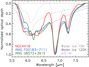
Figure 29: Comparison of the normalized 5.5–8 $\mu$m optical depth profiles of three galactic nuclei. Overlaid with dotted lines are the profiles of pure water ice and a a:C-H hydrogenated amorphous carbon analog.

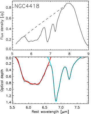
Figure 30: Absorption features in the 5–8 $\mu$m spectrum of NGC 4418. Upper panel: the Spitzer-IRS low-resolution spectrum of NGC 4418 (Spoon et al., 2007) with the local 5.6–7.8 $\mu$m absorption-corrected continuum shown as a dashed line. Lower panel: Optical depth spectrum resulting from adopting the local 5.6–7.8 $\mu$m spline continuum shown in the upper panel. Overlaid in red is the 6 $\mu$m water ice profile and overlaid in blue is the aliphatic CH deformation mode feature to be used for fitting IDEOS spectra.

We therefore resorted to using an empirical optical depth profile as our template, and separated the contribution of the CH deformation modes at 6.85 & 7.25 $\mu$m from the rest of the optical depth profile (6 $\mu$m profile hereafter) to maximise the ability to fit these features in other IDEOS spectra. We chose the spectrum of NGC 4418 as our template, over the spectra of IRAS F00183–7111 and IRAS 08572+3915, because its more symmetric 6 $\mu$m profile provides better fits to most spectra than the highly asymmetric 6 $\mu$m profiles of IRAS F00183–7111 and IRAS 08572+3915 (Fig. 29).

Following Dartois et al. (2007), we fit the 6.85 and 7.25 $\mu$m aliphatic CH deformation absorption bands with gaussian profiles and subtract these from the optical depth spectrum. The remaining optical depth profile in the 5.6–6.7 $\mu$m range is then attributed to 6 $\mu$m water ice and is smoothed so that it can be used as a water ice template for fitting IDEOS spectra. This profile is overlaid in red in the lower panel of Fig. 30. The blue profile in the same panel is the combined aliphatic CH deformation mode profile.

Appendix B PAH profile templates

The PAH emission features at 6.22, 11.25 and 12.65 $\mu$m (PAH62, PAH112, and PAH127) have asymmetric profiles, requiring either a combination of gaussian probability functions, or a single asymmetric probability function to accurately describe the observed shapes.

We chose the type IV probability function of Pearson (1895), used to model pull distributions with non-gaussian tails, for our purposes. The functional form for this Pearson-IV profile, P(x), is as follows:

$$P(x)=k\ [1+(\frac{x-\lambda}{a})^{2}\ ]^{-m}\ {\rm exp}[\ -\nu\ {\rm tan}^{-1}(\frac{x-\lambda}{a})\ ]$$ (B1)

where the normalization coefficient k is defined by Heinrich (2004) for m$>$1/2 as:

$$k=\frac{1}{\sqrt{\pi}\ a}\ \frac{\Gamma(m)}{\Gamma(m-1/2)}\ \left|\frac{\Gamma(m\ +\ i\nu/2)}{\Gamma(m)}\right|^{2}$$ (B2)

where $\Gamma$ is defined as

$$\Gamma(x)=\int_{0}^{\infty}t^{x-1}\ e^{-t}\ dt$$ (B3)

The last term in Eq. B2 can be computed using a piece of computer code, GAMMAR2, provided in Sect. 5.1 of Heinrich (2004).

Table 9 shows for each of the three PAH profiles the allowed parameter ranges for the four parameters in the Pearson-IV function. Only $a$ and $\lambda$ are allowed to vary. The former to accommodate the variation in width of the PAH feature resulting from the factor $\sim$2 variation in spectral resolution. The latter to allow compensation for the shift of the peak as a result of a change in $a$. See Fig. 31.

t PAH62 PAH112 PAH127 $\lambda$ 6.14–6.152 11.07–11.14 13.02–13.04 a 0.095–0.11 0.13–0.155 0.345–0.375 m 2.0 2.0 5.0 $\nu$ -2.5 -4.0 10.0

Table 9: Pearson IV parameters used to define shapes of PAH profiles

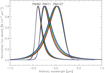
Figure 31: Normalized pearson-IV profiles used to model the PAH62, PAH112 and PAH127 features in the SED fitting of the 5.39–7.25 $\mu$m and 9.8–13.5 $\mu$m ranges. Different colors are used to show the effect of varying the A parameter within the allowed ranges.

Appendix C Crystalline silicate templates

Following Spoon et al. (2006), we attribute the 16.1, 18.5, 23.3, 27.6, and 33.2 $\mu$m absorption and emission bands seen in the IDEOS galaxy sample to forsterite crystalline silicates and fit these bands with the empirical profiles described below and as shown in Fig. 32.

Figure 32: Normalized optical depth profiles of crystalline silicates found in spectra of IDEOS galaxies. The panel of the left shows the profiles of the 16.1 and 18.5 $\mu$m forsterite bands, which are fitted together. The other forsterite bands, centered at 23.3, 27.6 and 33.2 $\mu$m, are fitted individually.

In Galactic sources the 16.1 $\mu$m forsterite band can be easily identified in the spectra of select young and old stars (Fig. 33), both in emission (e.g. T Tauri stars IRAS F12571–7657 and SSTc2d J033035.9+303024; see the spectra in Olofsson et al. (2009)) and in absorption (e.g. OH/IR stars IRAS 17347–2319, IRAS 17276–2846, and OH 21.5+0.5; see the spectra in Jones et al. (2012)). The band profile looks the same as in deeply obscured galactic nuclei (NGC 4418, IRAS 08572+3915, and IRAS 04454–4838), as can be seen in the inset of Fig. 33, after removal of the spline-fitted amorphous silicate component (Spoon et al., 2006). We therefore pick the 16.1 $\mu$m profile of the highest S/N galactic nucleus, IRAS 08572+3915, to serve as the profile to be used in the spectral fitting described in Sect. 3.5.

For some sources in Fig. 33 the strength of the 16.1 $\mu$m band is almost equal to the strength of the broader forsterite band peaking at 18.5–19 $\mu$m. The profile of the latter shows some variation among the galactic nuclei, with some sources peaking near 18.5 $\mu$m (e.g. IRAS 08572+3915 and IRAS 04454–4838) and others near 19.0 $\mu$m (e.g. NGC 4418). The latter is where the profiles of the stellar sources peak. Since the 16.1 and 18.5 $\mu$m forsterite features are fitted jointly with a fixed profile ratio, we choose the high S/N spectrum of IRAS 08572+3915 to also provide the template for the 18.5 $\mu$m forsterite profile.

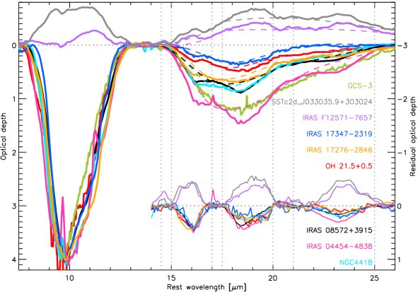
Figure 33: Silicate optical depth profiles of three deeply obscured galactic nuclei (NGC 4418, IRAS 08572+3915, and IRAS 04454-4838), five stellar sources (SSTc2d J033035.9+303024, IRAS F12571–7657, IRAS 17347–2319, IRAS 17276–2846, and OH 21.5+0.5 (Sloan et al., 2003)), and the Galactic Center Source GCS-3 (Chiar&Tielens, 2006). The silicate absorption spectra have been scaled to a 9.8 $\mu$m optical depth of 4. The silicate emission sources have not. The inset shows the residual optical depth features in the 14.5–26 $\mu$m range after subtraction of the spline-fitted amorphous silicate component (Spoon et al., 2006). GCS-3 is not included as it does not show crystalline signatures. For clarity, the residuals have been scaled to a common 16.1 $\mu$m absolute value.

The peak-to-peak profile ratio for the 16.1 and 18.5 $\mu$m bands in IRAS 08572+3915 is 1.0:0.83 (Fig. 32). This is far higher than calculated opacity curves for forsterite under various assumptions of grain size, grain shape, and optical constants predict. Take for example the forsterite opacity curves shown in Fig. 2 of de Vries et al. (2015), computed using the DHS grain shape distributions of Min et al. (2005) using optical constants of Suto et al. (2006); or the forsterite opacity curve shown in Fig. 2 of Spoon et al. (2006), which uses the optical constants of Fabian et al. (2001) and the assumption of a CDS grain shape distribution (Bohren et al., 1983). Invariably the 16.1 $\mu$m forsterite band is much weaker than the 19 $\mu$m band.

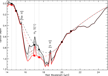
Figure 34: Optical depth profile for ESO 374-IG 032 NED02 in the 18 $\mu$m silicate absorption band (black). Dashed lines trace the amorphous 18 $\mu$m profile resulting from a spline fit to pivots at 14.5, 15.0, 17.0, 17.5, 20.0, and 21.0 $\mu$m. Residual optical depth features centered at 16.1, 18.5, and 23.3 $\mu$m are attributed to forsterite absorption. The profiles shown in red and in shades of gray are the result of subtracting the noise-free pure PAH template #3 of Smith et al. (2007) in increasing amounts.

This leads us to explore an alternative origin for the 16.1 and 18.5 $\mu$m absorption bands in galaxies, despite strong empirical evidence provided by the stellar spectra shown in Fig. 33. Could the appearance of 16.1 and 18.5 $\mu$m absorption features in the spectra of buried galactic nuclei be ascribed to the presence of PAH emission from the 17 $\mu$m PAH complex (Smith et al., 2007) instead? Fig. 34 shows the 14–25 $\mu$m spectrum of ESO 374-IG 032 NED02, a deeply obscured galactic nucleus with clear signs of PAH emission in the 6–13 $\mu$m range and at 16.4 and 17.4 $\mu$m. Using the noise-free PAH template #3 of Smith et al. (2007), we subtracted as much of the 17 $\mu$m PAH complex emission from the galaxy spectrum as is consistent with the amount of PAH emission found in the 6–13 $\mu$m range. As can be seen in Fig. 34, the 16.4 and 17.4 $\mu$m PAH bands disappear as the amount of subtracted PAH template emission increases, yet the 16.1 and 18.5 $\mu$m absorption structures remain even in the red spectrum, which represents moderate oversubtraction of 6–13 $\mu$m PAH emission. A full fit to the latter spectrum (the red dashed line in Fig. 34) would measure almost the same forsterite strength as a fit to the original spectrum would. We thus conclude that the 16.1 and 18.5 $\mu$m forsterite absorption bands cannot be mimicked by emission from the 17 $\mu$m PAH complex.

The profiles used to fit the 23.2 $\mu$m and the 27.6 $\mu$m forsterite bands in the 21.5–36 $\mu$m spectral range (Sect. 3.6) have been adapted from the average crystalline silicate optical depth spectrum of 12 ULIRGs obtained by Spoon et al. (2006). This average profile has higher S/N in the 21–30 $\mu$m range than the profile of IRAS 08572+3915. The resulting profiles, characteristic of forsterite, are shown in the middle panels of Fig. 32.

The profile of the 33.2 $\mu$m crystalline silicate band is best determined from high S/N spectra of galaxies in mid-IR classes 1A–C and 2A, which show the feature in emission. The galaxies we selected have the following IDEOS IDs: 10510592_0, 10511872_0, 10870272_0, 10871808_0, 11290112_1, 12432128_3, 14839552_0, 14840320_0, 14842112_0, and 14869504_0. To obtain the feature profile we first averaged the continuum-normalized spectra, and then removed the profile of the 33.48 $\mu$m [S iii] line. The resulting forsterite profile is shown in the right panel of Fig. 32.

References

- Armus et al. (2020) Armus, L., Charmandaris, V., Soifer, B.T., 2020, Nature Astronomy, 4, 467
- Asano et al. (2013) Asano, R.S., Takeuchi, T.T., Hirashita, H., Inoue, A.K., 2013, Earth Planets Space, 65, 213
- Bernard-Salas et al. (2009) Bernard-Salas, J., et al., 2009, ApJS, 184, 230
- Bohlin et al. (2011) Bohlin, R.C., et al., 2011, AJ, 141, 173
- Bohren et al. (1983) Bohren, C.F., Huffman, D.R., 1983, In: Absorption and scattering of light by small particles, New York: Wiley
- Boulanger et al. (1998) Boulanger, F., Boissel, P., Cesarsky, D., Ryter, C., 1998, A&A, 339, 194
- Bringa et al. (2007) Bringa, E.M., et al., 2007, ApJ, 662, 372
- Brown et al. (2014) Brown, M.J.I., Jarrett, T.H, Cluver, M.E., 2014, PASA, 31, 49
- Chiar&Tielens (2006) Chiar, J.E., Tielens, A.G.G.M., 2006, ApJ, 637, 774
- Colina et al. (2005) Colina, L., Arribas, S., Monreal-Ibero, A., 2005, A&A, 621, 725
- Dartois et al. (2005) Dartois, E., Muñoz Caro, G.M., Deboffle, D., Montagnac, G., d’Hendecourt, L., 2005, A&A, 432, 895
- Dartois et al. (2007) Dartois, E., et al., 2007, A&A, 463, 635
- Dasyra et al. (2008) Dasyra, K.M., et al., 2008, ApJ, 674, L9
- de Vries et al. (2014) de Vries, B.L., et al., 2014, A&A, 561, 75
- de Vries et al. (2015) de Vries, B.L., Maaskant, K.M., Min, M., Lombaert, R., Waters, L.B.F.M., Blommaert, J.A.D.L., 2015, A&A, 576, 98
- Diaz-Santos et al. (2010) Díaz-Santos, T., et al., 2010, ApJ, 723, 993
- Dijkstra et al. (2003) Dijkstra, C., et al., 2003, A&A, 399, 1037
- Dorschner et al. (1995) Dorschner, J., Begemann, B., Henning, T., Jäger, C., Mutschke, H., 1995, A&A, 300, 503
- Engelbracht et al. (2007) Engelbracht, C.W, 2007, PASP, 119, 994
- Fabian et al. (2001) Fabian, D., Henning, T., Jäger, C., Mutschke, H., Dorschner, J., Wehrhan, O., 2001, A&A, 378, 228
- Falstad et al. (2021) Falstad, N., et al., 2021, A&A, accepted (ASTRO-PH/2102.13563)
- Fuhrmann et al. (2006) Fuhrmann, L., et al., A&A, 445, L1
- Furlan et al. (2011) Furlan, E., et al., 2011, ApJS, 195, 3
- Galliano et al. (2008a) Galliano, F., Dwek, E., Chanial, P., 2008, ApJ, 672, 214
- Galliano et al. (2008b) Galliano, F., Madden, S.C., Tielens, A.G.G.M., Peeters, E., Jones, A.P., 2008, ApJ, 679, 310
- Gallimore et al. (2010) Gallimore, J.F., et al., 2010, ApJS, 187, 172
- Glasse et al. (2015) Glasse, A., et al., 2015, PASP, 127, 686
- Genzel et al. (1998) Genzel, R., et al., 1998, ApJ, 498, 579
- Golriz et al. (2014) Golriz, S.S., 2014, MNRAS, 443, 3402
- Gordon et al. (2008) Gordon, K., et al., 2008, ApJ682, 336
- Gorjian et al. (2007) Gorjian, V., Cleary, K., Werner, M.W., Lawrence, C.R., ApJ, 655, L73
- Hao et al. (2009) Hao, L., et al., 2009, ApJ, 704, 1159
- Hatziminaoglou et al. (2015) Hatziminaoglou E., Hernán-Caballero A., Feltre A., Piñol Ferrer N. 2015, ApJ, 803, 110
- Heinrich (2004) Heinrich, J., 2004, CDF memo 6820
- Hernán-Caballero et al. (2015) Hernán-Caballero A., et al. 2015, ApJ, 803, 109
- Hernán-Caballero et al. (2016) Hernán-Caballero, A., Spoon, H.W.W., Lebouteiller, V., Rupke, D.S.N., Barry, D.P., 2016, MNRAS, 455, 1796
- Hernán-Caballero et al. (2020) Hernán-Caballero, A., et al., 2020, MNRAS, 497, 4614
- Hony et al. (2000) Hony, S., Van Kerckhoven, C., Peeters, E., Tielens, A.G.G.M., Hudgins, D.M., Allamandola, L.J., 2000, A&A, 370, 1030
- Hony et al. (2001) Hony, S., Van Kerckhoven, C., Peeters, E., Tielens, A.G.G.M., Hudgins, D.M., Allamandola, L.J., 2001, A&A, 370, 1030
- Hony et al. (2011) Hony, S., et al., 2011, A&A, 531, 137
- Hopkins et al. (2006) Hopkins, P.F., Hernquist, L., Cox, T., et al., 2006, ApJS, 163, 1
- Houck et al. (2004) Houck, J.R., et al. 2004, ApJS, 154, 18
- Jones et al. (1994) Jones, A.P., Tielens, A.G.G.M., Hollenbach, D.J., McKee, C.F., 1994, ApJ, 433, 797
- Jones et al. (1996) Jones, A.P., Tielens, A.G.G.M., Hollenbach, D.J., 1996, ApJ, 469, 740
- Jones et al. (2012) Jones, O.C., et al., 2012, MNRAS, 427, 3209
- Kemper et al. (2004) Kemper, F., Vriend, W.J., Tielens, A.G.G.M., 2004, ApJ, 609, 826
- Kemper et al. (2005) Kemper, F., Vriend, W.J., Tielens, A.G.G.M., 2005, ApJ, 633, 534
- Koornneef et al. (1986) Koornneef, J., Bohlin, R., Buser, R., Horne, K., Turnshek, D., 1986, in Proc. IAU XIX General Assembly, Highlights of Astronomy Vol. 7, ed. J.-P. Swings (Washington, DC: AURA), 833
- Lahuis et al. (2007) Lahuis, F., et al., 2007, ApJ, 659, 296
- Laurent et al. (2000) Laurent, O., et al., 2000, A&A, 359, 887
- Lebouteiller et al. (2011) Lebouteiller, V, Barry, D.J., Spoon, H.W.W., Bernard-Salas, J., Sloan, G.C., Houck, J.R., Weedman, D.W., 2011, ApJS, 196, 8
- Lutz (1996) Lutz, D., et al., 1996, A&A, 315, L269
- Markwardt (2009) Markwardt, C.B., 2009, Astronomical Data Analysis Software and Systems XVIII, 411, 251
- Marshall et al. (2007) Marshall, J.A., Herter, T.L., Armus, L., Charmandaris, V., Spoon, H.W.W., Bernard-Salas, J., Houck, J.R., 2007, ApJ, 670, 129
- Marshall et al. (2018) Marshall, J.A., Elitzur, M., Armus, L., Diaz-Santos, T., Charmandaris, V., 2018, ApJ, 858, 59
- Meeus et al. (2001) Meeus, G., et al., 2001, A&A, 365, 476
- Meixner et al. (2002) Meixner, M., Ueta, T., Bobrowsky, M., Speck, A., 2002, ApJ, 571, 936
- Min et al. (2005) Min, M., Hovenier, J.W., de Koter, A., A&A, 432, 909
- Min et al. (2009) Min, M., Dullemond, C.P., Dominik, C., de Koter, A., Hovenier, J.W., 2009, A&A, 497, 155
- Molster & Kemper (2005) Molster, F., Kemper, C., 2005, Space Science Reviews, 119, 3
- Nenkova et al. (2002) Nenkova, M., Ivezíc, Z., Elitzur, M., 2002, ApJ, 570, 9
- Oliva et al. (1999) Oliva, E., Moorwood, A.F.M., Drapatz, S., Lutz, D., Sturm, E., 1999, A&A, 343, 943
- Olofsson et al. (2009) Olofsson, J., et al., 2009, A&A, 507, 327
- Ossenkopf et al. (1992) Ossenkopf, V., Henning, T., & Mathis, J.S. 1992, A&A, 261, 567
- Pearson (1895) Pearson, K., 1895, Philosophical Transactions of the Royal Society of London A, 186,343
- Peeters et al. (2004) Peeters, E., Spoon, H.W.W., Tielens, A.G.G.M., 2004, ApJ, 613, 986
- Peréz-Beaupuits et al. (2011) Peréz-Beaupuits, J.P., Spoon, H.W.W., Spaans, M., Smith, J.D., 2011, A&A, 533, 56
- Reach et al. (2005) Reach, W.T., et al., 2005, PASP, 117, 978
- Rogantini et al. (2019) Rogantini, D., et al., 2019, A&A, 630, 143
- Rogantini et al. (2020) Rogantini, D., et al., 2020, A&A, 641, 149
- Roussel et al. (2006) Roussel, H., et al., 2006, ApJ, 646, 841
- Rowan-Robinson et al. (2009) Rowan-Robinson, M., Efstathiou, A., 2009, MNRAS, 399, 615
- Rupke et al. (2021) Rupke, D.S.N., Schweitzer, M., Viola, V., Lutz, D., Sturm, E., Spoon, H.W.W., Veilleux, S., Kim, D.-C., 2021, ASCL, https://doi.org/10.5281/zenodo.5781471
- Sanders & Mirabel (1996) Sanders, D.B., Mirabel, I.F., 1996, ARA&A, 34, 749
- Schweitzer et al. (2008) Schweitzer, M., et al., 2008, ApJ, 679, 101
- Sirocky et al. (2008) Sirocky, M.M., Levenson, N.A., Elitzur, M., Spoon, H.W.W., Armus, L., 2008, ApJ, 678, 729
- Sloan et al. (2003) Sloan, G.C., Kraemer, K.E., Price, S.D., Shipman, R.F., 2003, ApJS, 147, 379
- Smith et al. (2007) Smith, J.D.T., et al., 2007, ApJ, 656, 770
- Spoon et al. (2000) Spoon, H.W.W., Koornneef, J., Moorwood, A.F.M., Lutz, D., Tielens, A.G.G.M., A&A357, 898
- Spoon et al. (2001) Spoon, H.W.W., Keane, J.V., Tielens, A.G.G.M., Lutz, D., Moorwood, A.F.M., 2001, A&A, 365, L353
- Spoon et al. (2003) Spoon, H.W.W., Moorwood, A.F.M., Pontoppidan, K.M., Cami, J., Kregel, M., Lutz, D., Tielens, A.G.G.M., 2003, A&A, 402, 499
- Spoon et al. (2004) Spoon, H.W.W., et al., 2004, ApJS, 154, 184
- Spoon et al. (2006) Spoon, H.W.W., et al., 2006, ApJ, 638, 759
- Spoon et al. (2007) Spoon, H.W.W., et al., 2007, ApJ, 654, L49
- Spoon et al. (2009a) Spoon, H.W.W., Armus, L., Marshall, J.A., Bernard-Salas, J., Farrah, D., Charmandaris, V., Kent, B.R., 2009, ApJ, 693, 1223
- Spoon et al. (2009b) Spoon, H.W.W., Holt, J., 2009, ApJ, 702, L42
- Suto et al. (2006) Suto, H., et al., 2006, MNRAS, 370, 1599
- Sylvester et al. (1999) Sylvester, R.J., et al., 1999, A&A, 352, 587
- Van Loon et al. (2015) Van Loon, J.T., Sansom, A.E., 2015, MNRAS, 453, 2341
- Varenius et al. (2017) Varenius, E., et al., 2017, A&A, accepted
- Veilleux et al. (2009) Veilleux, S., et al., 2009, ApJS, 182, 628
- Vermeij et al. (2002) Vermeij, R., Peeters, E., Tielens, A.G.G.M., van der Hulst, J.M., 2002, A&A, 382, 1042
- Watson et al. (2009) Watson, D.M., et al., 2009, ApJS, 180, 84
- Werner et al. (2004) Werner, M.W., et al., 2004, ApJS, 154, 1
- Wright et al. (2010) Wright, E.L., et al., 2010, AJ, 140, 1868
- Xie et al. (2014) Xie, Y., Hao, L., Li, A., 2014, ApJ, 794, 19
- Zeegers et al. (2019) Zeegers, S.T., Costantini, E., Rogantini, D., et al., 2019, A&A, 627, 16
- Zubko et al. (1996) Zubko, V.G., Mennella, V., Colangeli, L., Bussoletti, E., 1996, MNRAS, 282, 1321