A generalised time-evolution model for
contact problems with wear and its analysis

Dmitry Ponomarev1,2,3
Abstract.

In this paper, we revisit some classical and recent works on modelling sliding contact with wear and propose their generalisation. Namely, we upgrade the relation between the pressure and the wear rate by incorporating some non-local time-dependence. To this effect, we use a combination of fractional calculus and relaxation effects. Moreover, we consider a possibility when the load is not constant in time. The proposed model is analysed and solved. The results are illustrated numerically and comparison with similar models is discussed.

1. Introduction

11footnotetext: FACTAS team, Centre Inria d’Université Côte d’Azur, France22footnotetext: St. Petersburg Department of Steklov Mathematical Institute of Russian Academy of Sciences, Russia33footnotetext: Contact: dmitry.ponomarev@inria.fr

Wear of material is a complicated process which involves different phenomena such as abrasion, adhesion and crack formation. Wear processes have been studied for decades and numerous empirical models have been proposed in attempt to fit experimental data for particular settings. One classical model of wear is due to Archard [6]. According to this model, the wear rate is proportional to the load with a power-law dependence. In many settings, this reduces to a linear relation between the wear rate and the pressure (see e.g. [32, Sect. 17.2–17.3]) leading to several effectively solvable tribological models for sliding of an indented punch (stamp), see e.g. [9, 10, 11, 15, 25, 41]. It seems natural to explore a larger class of such models based on a more general relation between the wear rate and the contact pressure. A qualitative upgrade of this relation could be achieved by accounting for non-local (temporal) dependencies. Investigation of how a new wear model affects the solution of a problem would give a hope to extend the applicability of original models to contexts with different wear mechanisms and a broader set of materials.

Here, we consider the following instance of the two-dimensional punch problem: a rigid wearable punch, subject to a given normal (vertical) load, slides on a thick elastic layer or a half-plane, with a prescribed speed. The sliding speed is taken to be constant, but the normal load may be time-dependent. The contact area is assumed to be fixed (which is normally expected if the load is sufficiently large, see e.g. [26]).

Since the layer is homogeneous and material wear occurs on the interface, the problem can be effectively described by one-dimensional integral equations. On this level, the presence of wear in the problem manifests itself as an additional term in the integral equation for the pressure. This term stems from the linear Archard’s wear law and brings a temporal dependence to the problem.

In the present work, we upgrade the wear term so that it corresponds to a more general differential relation between the wear rate and the contact pressure. This more general relation is meant to have two features (and combinations thereof). First, it incorporates a wear-relaxation effect which is consistent with typical observations that wear is the most intense in the beginning of the sliding process. Second, the time-derivative in this relation may be changed to a fractional order (in a Riemann-Liouville sense) which adds another non-locality and is motivated by recent success of fractional calculus in mechanics (viscoelasticity) and other applied contexts [19, Ch. 9–10]. Importance of non-local relations between wear and contact pressure is also stressed in recent work [8].

As we shall see, newly introduced parameters can affect qualitative behaviour of the solution. Namely, depending on a choice of the parameter values, the solution may exhibit exponential or algebraic decay in time that would range between monotone and arbitrary oscillatory. Therefore, such a generalised model is highly desirable and is expected to be useful for fitting experimentally observable data. On the other hand, this model is almost explicitly solvable, meaning that the solution can be written up in a closed form in terms of some auxiliary functions which could be precomputed (numerically or asymptotically). In particular, it is rather straightforward to analyse long-time behaviour of this model, namely, its convergence speed to the stationary pressure distribution. Moreover, computing such a pressure profile itself is a problem of an essential practical interest.

The outline of the paper is as follows. We formulate a new model in Section 2. In Section 3, we derive the proposed form of the wear relation and recast the model in form of a single integral equation. Then, in Section 4, we deal with the solution of the general model and its analysis. In particular, in Subsection 4.2, under appropriate conditions, we deduce the existence of a unique solution and provide its explicit form in terms of spectral functions of a pertinent integral operator. This is detailed even more for a concrete choice of the kernel function in Subsection 4.3. Furthermore, in Section 5, we show that the solution of the proposed model has the anticipated behaviour consistent with previous models. A collection of mathematical results needed for Sections 45 is outsourced to Appendix. Section 6 is dedicated to the numerical solution of the proposed model: its validation and exploration. Finally, we conclude with Section 7 where we summarise and discuss the results outlining potential further work.

2. The model

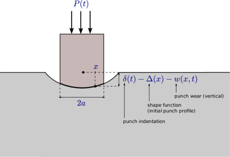
According to [3, 9, 10, 11, 18, 26, 39], a balance of displacements at the contact interface (see Figure 2.1) yields an integral equation which involves two unknowns: the contact pressure $p\left(x,t\right)$ and the indentation $\delta\left(t\right)$. This equation can be formulated as follows

(2.1) $$\eta\left(p\left(x,t\right)-p\left(x,0\right)\right)+\int_{-a}^{a}K\left(x-\xi\right)\left(p\left(\xi,t\right)-p\left(\xi,0\right)\right)\mathrm{d}\xi+w\left[p\right]\left(x,t\right)=\delta\left(t\right)-\delta\left(0\right),\hskip 10.00002ptx\in\left(-a,a\right),\hskip 10.00002ptt>0.$$

Furthermore, (2.1) should be complemented by the equilibrium condition

(2.2) $$\int_{-a}^{a}p\left(x,t\right)\mathrm{d}x=P\left(t\right),\hskip 10.00002ptt\geq 0,$$

and the integral equation for the initial pressure distribution $p\left(x,0\right)$

(2.3) $$\eta p\left(x,0\right)+\int_{-a}^{a}K\left(x-\xi\right)p\left(\xi,0\right)\mathrm{d}\xi=\delta\left(0\right)-\Delta\left(x\right),\hskip 10.00002ptx\in\left(-a,a\right).$$

Here, $K\left(x\right)$ is a given function which links the contact pressure to the vertical displacement, $\eta\geq 0$ is a given constant, $\left(-a,a\right)$ is the contact interval, $P\left(t\right)>0$ is the contact load, $w\left[p\right]\left(x,t\right)$ is the wear term which is a given mapping of the contact pressure $p\left(x,t\right)$ and the punch profile $\Delta\left(x\right)$ is a known function.

The main feature of our model is a new form of the wear term $w\left[p\right]\left(x,t\right)$ entering (2.1). This wear term is given by

(2.4) $$w\left[p\right]\left(x,t\right)=-\nu\mu^{1/\alpha-1}\int_{0}^{t}\mathcal{E}_{\alpha}\left(\mu^{1/\alpha}\left(t-\tau\right)\right)p\left(x,\tau\right)\mathrm{d}\tau,$$

where $\mathcal{E}_{\alpha}$ is an auxiliary function defined by (A.7) and $\mu>0$, $\alpha\in\left(0,2\right)$ are given constants.

Refer to caption
Figure 2.1. Geometry of the problem. A balance of displacements under the punch is governed by the equation: $\eta p\left(x,t\right)+\int_{-a}^{a}K\left(x-\xi\right)p\left(\xi,t\right)\mathrm{d}\xi=\delta\left(t\right)-\Delta\left(x\right)-w\left(x,t\right)$, $x\in\left(-a,a\right)$, $t\geq 0$.

Relation to other models

The considered model is an amalgam as it attempts to treat different settings at once as we shall discuss here.

First of all, we perform most of the analysis for a rather general form of the kernel function $K\left(x\right)$ entering (2.1) and (2.3) while only making some assumptions on it. This allows dealing with an elastic half-plane or an elastic layer subject to different boundary conditions at its foundation, see e.g. [1, 2, 39, Par. 11]. In Subsection 4.3, we also provide a more detailed study for a concrete kernel function pertinent to the half-plane geometry.

Works [11, 9, 10, 26] involve counterparts of (2.1) and (2.3) with $\eta=0$. The case $\eta>0$ accounts for the surface roughness effect or coating [4, 25] which is due to an additional deformation proportional to the local pressure [37, Ch. 2 Par. 8]. We note that some aspects of the solution construction and its analysis differ depending on whether $\eta=0$ or $\eta>0$, and this will be reflected in our formulations of theorems and propositions given in Sections 45.

In most settings, $P\left(t\right)\equiv P_{0}$ was taken in (2.2) for some constant $P_{0}>0$. A possibility of a non-constant load is mentioned in [9] but not studied. We study the more general load since, on the one hand, it appears to be of a direct physical interest and, on the other hand, the presented solution of the model can be adapted for this case, even though some computational details become more cumbersome. Despite this generality, we perform a more concrete analysis (see Section 5) for two particular type of loads: the most important case of a constant load and the case of a transitional load (when the load may vary in time but is eventually constant).

We shall now briefly discuss some relevant works that would motivate our new model based on a peculiar choice of the wear term.
As discussed in Section 1, a simple but powerful version of the wear term is derived from the linear Archard’s law. According to this relation, the wear is linearly proportional to the total sliding distance and the contact pressure. Consequently, we have

(2.5) $$\partial_{t}w\left(x,t\right)=\nu p\left(x,t\right)$$

for some constant $\nu>0$ related to the material and the sliding speed. Hence, since at the initial moment $t=0$ the worn material is absent, i.e. $w\left(x,0\right)\equiv 0$ for $x\in\left(-a,a\right)$, (2.5) is equivalent to

(2.6) $$w\left[p\right]\left(x,t\right)\equiv w\left(x,t\right)=\nu\int_{0}^{t}p\left(x,\tau\right)\mathrm{d}\tau.$$

Recently, in [9], the authors considered a generalised version of (2.6), namely,

$$w\left[p\right]\left(x,t\right)=k_{0}\left(x\right)\int_{0}^{t}p\left(x,\tau\right)\mathrm{d}\tau$$

for some suitable function $k_{0}\left(x\right)$. Another generalisation was proposed in [7] which, in its simple form, corresponds to

$$w\left[p\right]\left(x,t\right)=\int_{0}^{t}k_{1}\left(\tau\right)p\left(x,\tau\right)\mathrm{d}\tau,$$

but can also include additional dependencies of $k_{1}$.

Numerous models with nonlinear wear have been considered, in this case we have (see e.g. [41] and [21, eq. (6.82)])

$$w\left[p\right]\left(x,t\right)=\nu\int_{0}^{t}p^{\gamma}\left(x,\tau\right)\mathrm{d}\tau,$$

with some nonlinearity parameter $\gamma>0$.

Finally, we mention that, in addition to the wear term, the friction effects were also considered in [10], by incorporating in (2.1) another term proportional to $\int_{-a}^{x}p\left(\xi,t\right)\mathrm{d}\xi$.

3. Derivation of the model

While the generalisation of the previous setting by including an extra term proportional to the solution and allowing load to vary in time is natural, choosing a complicated looking wear term is a nontrivial feature of the present model that we shall now discuss.

3.1. Towards the wear term (2.4)

We consider a generalisation of (2.5)–(2.6) that can be obtained in two independent steps.
First, we add to the right-hand side of (2.5) a term $-\mu w\left(x,t\right)$ with some constant $\mu\geq 0$. This would result in (2.6) being replaced by

(3.1) $$w\left[p\right]\left(x,t\right)=\nu\int_{0}^{t}e^{-\mu\left(t-\tau\right)}p\left(x,\tau\right)\mathrm{d}\tau,$$

where we took into account the condition $w\left(x,0\right)=0$ representing the initial absence of the worn material. We note that models with such a hereditary wear term has already been considered, see e.g. [40].
At the second step, we replace the differentiation in time in the left-hand side of (2.5) with a more general notion of the derivative. In particular, we use the fractional Riemann-Liouville derivative of order $\alpha\in\left(0,1\right]$ (for the values $\alpha>1$ see remark at the end of the paragraph) that we denote $D_{t}^{\alpha}$, namely,

(3.2) $$D_{t}^{\alpha}w\left(x,t\right):=\frac{1}{\Gamma\left(1-\alpha\right)}\frac{\partial}{\partial t}\int_{0}^{t}\frac{w\left(x,\tau\right)}{\left(t-\tau\right)^{\alpha}}\mathrm{d}\tau,$$

where $\Gamma$ denotes Gamma function defined in Appendix. Note that, due to the condition $w\left(x,0\right)=0$, this derivative would also coincide with the fractional Caputo derivative (see e.g. [20, eq. (1.19)]).

In other words, we choose to generalise (2.5) to the following non-homogeneous fractional order ODE

(3.3) $$D_{t}^{\alpha}w\left(x,t\right)=-\mu w\left(x,t\right)+\nu p\left(x,t\right).$$

We are now going to obtain the integral form of (3.3) and hence the corresponding relation $w\left[p\right]\left(x,t\right)$. To this end, we set $\tilde{t}:=\mu^{1/\alpha}t$, $\tilde{w}\left(x,\tilde{t}\right):=w\left(x,\tilde{t}/\mu^{1/\alpha}\right)$, $\tilde{p}\left(x,\tilde{t}\right):=p\left(x,\tilde{t}/\mu^{1/\alpha}\right)$. Then, relation (3.3) rewrites as

(3.4) $$D_{\tilde{t}}^{\alpha}\tilde{w}\left(x,\tilde{t}\right)=D_{\tilde{t}}^{\alpha}\left(\tilde{w}\left(x,\tilde{t}\right)-\tilde{w}\left(x,0\right)\right)=-\tilde{w}\left(x,\tilde{t}\right)+\frac{\nu}{\mu}\tilde{p}\left(x,\tilde{t}\right),$$

where we used that $\tilde{w}\left(x,0\right)=w\left(x,0\right)=0$. A fractional differential equation in the form (3.4) is solved in [20, eq. (3.13)] using Laplace transforms. Taking into account that $\tilde{w}\left(x,0\right)=0$ and $\alpha\in\left(0,1\right]$, the obtained solution is

$$\tilde{w}\left(x,\tilde{t}\right)=-\frac{\nu}{\mu}\int_{0}^{\tilde{t}}\tilde{p}\left(x,\tilde{t}-\tilde{\tau}\right)\mathcal{E}_{\alpha}\left(\tilde{\tau}\right)\mathrm{d}\tilde{\tau}.$$

Therefore,

(3.5) $$w\left[p\right]\left(x,t\right)=\tilde{w}\left(x,\mu^{1/\alpha}t\right)=-\nu\mu^{1/\alpha-1}\int_{0}^{t}p\left(x,t-\tau\right)\mathcal{E}_{\alpha}\left(\mu^{1/\alpha}\tau\right)\mathrm{d}\tau,$$

and thus (2.4) follows. Observe that the assumed range $\alpha\in\left(0,1\right]$ can be extended to values $\alpha>1$ as relation (2.4) remain meaningful (note, however, that definition (3.2) should be replaced with a more general one [20, eq. (1.13)]).

Equations (2.1)–(2.3) together with the wear term given by (2.4) constitute the general model proposed in the present work.

3.2. Consistency

It is noteworthy that when $\mu=0$ in (3.3), we take the limit $\mu\rightarrow 0$ in (2.4). In doing so, we use the asymptotics (A.14) to obtain

(3.6) $$w\left[p\right]\left(x,t\right)=\frac{\alpha\nu}{\Gamma\left(1+\alpha\right)}\int_{0}^{t}p\left(x,t-\tau\right)\tau^{\alpha-1}\mathrm{d}\tau=\frac{\nu}{\Gamma\left(\alpha\right)}\int_{0}^{t}\frac{p\left(x,\tau\right)}{\left(t-\tau\right)^{1-\alpha}}\mathrm{d}\tau.$$

The right-hand side of (3.6) contains the Riemann-Liouville integral of order $\alpha$ which is consistent with the inversion of the respective fractional derivative appearing in (3.3) (see [20, eqs. (1.29), (1.2)]).

On the other hand, by taking $\alpha=1$ in (2.4), we have $\mathcal{E}_{1}\left(z\right)=-e^{-z}$, and hence we recover the non-fractional order model corresponding to (3.1).

Hence, our present model can be succinctly characterised as a model with the wear term interpolating between the exponential relaxation and a new fractional order model.

3.3. The integral equation

Equations (2.1)–(2.3) with the wear term (2.4) can be effectively reduced to a single equation. To achieve that, we integrate (2.1) in the $x$ variable over $\left(-a,a\right)$ and use (2.2) and (2.4). This yields

(3.7) $$\eta\left(P\left(t\right)-P\left(0\right)\right)+\int_{-a}^{a}K_{1}\left(\xi\right)\left(p\left(\xi,t\right)-p\left(\xi,0\right)\right)\mathrm{d}\xi-\nu\mu^{1/\alpha-1}\int_{0}^{t}\mathcal{E}_{\alpha}\left(\mu^{1/\alpha}\left(t-\tau\right)\right)P\left(\tau\right)\mathrm{d}\tau=2a\left(\delta\left(t\right)-\delta\left(0\right)\right),\hskip 10.00002ptt>0,$$

where we introduced the function $K_{1}\left(\xi\right):=\int_{-a}^{a}K\left(\zeta-\xi\right)\mathrm{d}\zeta$.

Dividing (3.7) over $2a$ and subtracting the resulting equation from (2.1), we eliminate $\delta\left(t\right)-\delta\left(0\right)$ and obtain, for $x\in\left(-a,a\right)$, $t>0$,

(3.8) $\displaystyle\eta\left(p\left(x,t\right)-p\left(x,0\right)-\frac{P\left(t\right)-P\left(0\right)}{2a}\right)+\int_{-a}^{a}\left[K\left(x-\xi\right)-\frac{1}{2a}K_{1}\left(\xi\right)\right]\left(p\left(\xi,t\right)-p\left(\xi,0\right)\right)\mathrm{d}\xi=$
$\displaystyle=\frac{\nu}{\mu^{1-1/\alpha}}\int_{0}^{t}\mathcal{E}_{\alpha}\left(\mu^{1/\alpha}\left(t-\tau\right)\right)\left(p\left(x,\tau\right)-\frac{P\left(\tau\right)}{2a}\right)\mathrm{d}\tau.$

This is an integral equation featuring only one unknown $p\left(x,t\right)$. Note that $p\left(x,0\right)$ can be assumed to be known from solving (2.3) with the unknown $\delta\left(0\right)$ that is found a posteriori from condition (2.2) imposed at $t=0$. As we shall further discuss in Subsection 4.2 (see Corollary 8), the assumption on the knowledge of $p\left(x,0\right)$ does not restrict generality as long as $\eta>0$.

The obtained relation (3.8) is an integral equation of the mixed type in two variables: it contains both Fredholm and Volterra integral operators in the spatial and temporal parts, respectively.

4. Solution by separation of variables

Since temporal and spatial operators appearing in equation (3.8) are not intertwined, it is natural to attempt solving the problem with the method of separation of variables. Therefore, we first focus on the spatial part of the problem and study the appropriate functional setting for its solution.

4.1. Notation, assumptions and their implications

We start by fixing the notation. We shall use $L^{p}\left(-a,a\right)$ to denote the space of all real-valued functions on $\left(-a,a\right)$ whose $p$-th power is Lebesgue integrable on the interval $\left(-a,a\right)$. In particular, $L^{2}\left(-a,a\right)$ is a Hilbert space endowed with the inner product and norm defined as

(4.1) $$\left\langle f,g\right\rangle:=\int_{-a}^{a}f\left(x\right)g\left(x\right)\mathrm{d}x,\hskip 10.00002pt\left\|f\right\|:=\sqrt{\left\langle f,f\right\rangle},\hskip 10.00002ptf,g\in L^{2}\left(-a,a\right).$$

We will also need the space $L_{0}^{2}\left(-a,a\right)$ a subspace of $L^{2}\left(-a,a\right)$ that consists of all square-integrable functions with vanishing mean value on $\left(-a,a\right)$, i.e.

(4.2) $$L_{0}^{2}\left(-a,a\right):=\left\{f\in L^{2}\left(-a,a\right):\;\int_{-a}^{a}f\left(x\right)\mathrm{d}x=0\right\}.$$

Note that $L_{0}^{2}\left(-a,a\right)$ is a closed subspace of $L^{2}\left(-a,a\right)$, and hence is also a Hilbert space. Given $T>0$, let us denote $C_{b}\left(\left[0,T\right]\right)$, $C_{b}\left(\mathbb{R}_{+}\right)$ the spaces of bounded continuous functions on the closed interval $\left[0,T\right]$ and the positive half-line $\mathbb{R}_{+}:=\left[0,\infty\right)$.

Assumption 1 (Parity and real-valuedness).

Suppose that $K\left(x\right)$ is a real-valued even function on $\left(-a,a\right)$:

$$K\left(-x\right)=K\left(x\right)\in\mathbb{R},\hskip 10.00002ptx\in\left(-a,a\right).$$
Assumption 2 (Hilbert-Schmidt regularity).

Suppose that $K\left(x\right)$ is sufficiently regular, namely, we assume validity of the following integrability condition:

$$\int_{-a}^{a}\int_{-a}^{a}\left[K\left(x-\xi\right)\right]^{2}\mathrm{d}x\mathrm{d}\xi<\infty.$$
Assumption 3 (Positive semidefiniteness).

We suppose that, for any function $f\in L^{2}\left(-a,a\right)$, the following condition holds true:

$$\int_{-a}^{a}f\left(x\right)\int_{-a}^{a}K\left(x-\xi\right)f\left(\xi\right)\mathrm{d}\xi\mathrm{d}x\geq 0.$$

Because of Assumption 2, the condition of Lemma 17 is satisfied, and therefore the integral transformation given by

(4.3) $$f\mapsto\mathcal{K}\left[f\right]\left(x\right):=\int_{-a}^{a}K\left(x-\xi\right)f\left(\xi\right)\mathrm{d}\xi$$

defines a compact linear operator $\mathcal{K}:$ $L^{2}\left(-a,a\right)\rightarrow L^{2}\left(-a,a\right)$. Moreover, due to Assumption 1, this operator is self-adjoint. Consequently, by the spectral theory for compact self-adjoint operators (Lemma 18), it follows that, for any $f\in L^{2}\left(-a,a\right)$, we can write

(4.4) $$f\left(x\right)=\sum_{n=1}^{\infty}f_{n}\varphi_{n}\left(x\right)+f_{\perp}\left(x\right),$$

where $f_{\perp}\left(x\right)\in\text{Ker }\mathcal{K}$ and $\varphi_{n}\left(x\right)$, $n\geq 1$, are normalised eigenfunctions of the operator $\mathcal{K}$ with non-zero eigenvalues. In other words, we have

(4.5) $$\int_{-a}^{a}K\left(x,\xi\right)f_{\perp}\left(\xi\right)\mathrm{d}\xi=0,\hskip 10.00002ptx\in\left(-a,a\right),$$

and

(4.6) $$\int_{-a}^{a}K\left(x,\xi\right)\varphi_{n}\left(\xi\right)\mathrm{d}\xi=\lambda_{n}\varphi_{n}\left(x\right),\hskip 10.00002ptx\in\left(-a,a\right),$$

with some $\lambda_{n}\neq 0$, $n\geq 1$, which are eigenvalues (in general, repeated sequentially according to their multiplicity).

Setting

(4.7) $$K_{2}\left(x,\xi\right):=K\left(x-\xi\right)-\frac{1}{2a}K_{1}\left(x\right)-\frac{1}{2a}K_{1}\left(\xi\right),\hskip 10.00002pt\hskip 10.00002ptK_{1}\left(x\right):=\int_{-a}^{a}K\left(\zeta-x\right)\mathrm{d}\zeta,$$

we observe that

(4.8) $$\int_{-a}^{a}K_{2}\left(x,\xi\right)\mathrm{d}x=-\frac{1}{2a}\int_{-a}^{a}K_{1}\left(x\right)\mathrm{d}x=:c_{0},$$

The right-hand side of (4.8) is constant (independent of $\xi$), and hence, we obtain a relation

(4.9) $$\int_{-a}^{a}\int_{-a}^{a}K_{2}\left(x,\xi\right)\mathrm{d}\xi\mathrm{d}x=-\int_{-a}^{a}K_{1}\left(x\right)\mathrm{d}x.$$

Moreover, for any $f\in L_{0}^{2}\left(-a,a\right)$, we have

$$\int_{-a}^{a}\int_{-a}^{a}K_{2}\left(x,\xi\right)f\left(\xi\right)\mathrm{d}\xi\mathrm{d}x=0.$$

Therefore, using Lemma 17, we can define $\mathcal{K}_{2}:$ $L_{0}^{2}\left(-a,a\right)\rightarrow L_{0}^{2}\left(-a,a\right)$, a compact linear operator that corresponds to the integral transformation with the kernel function $K_{2}\left(x,\xi\right)$:

(4.10) $$f\mapsto\mathcal{K}_{2}\left[f\right]\left(x\right):=\int_{-a}^{a}K_{2}\left(x,\xi\right)f\left(\xi\right)\mathrm{d}\xi.$$

By the symmetry of $K_{2}\left(x,\xi\right)$, the operator $\mathcal{K}_{2}$ is self-adjoint and hence, using Lemma 18, we deduce that, for any $f\in L_{0}^{2}\left(-a,a\right)$, we can write

(4.11) $$f\left(x\right)=\sum_{n=1}^{\infty}\widetilde{f}_{n}\phi_{n}\left(x\right)+\widetilde{f}_{\perp}\left(x\right),$$

where $\widetilde{f}_{n}:=\left\langle f,\phi_{n}\right\rangle$, $\widetilde{f}_{\perp}:=f-\sum_{n=1}^{\infty}\widetilde{f}_{n}\phi_{n}\in\text{Ker }\mathcal{K}_{2}$, and $\phi_{n}$, $n\geq 1$, are normalised (i.e. $\left\|\phi_{n}\right\|=1$, $n\geq 1$) eigenfunctions of the operator $\mathcal{K}_{2}$ with non-zero eigenvalues. That is, we have

(4.12) $$\int_{-a}^{a}K_{2}\left(x,\xi\right)\widetilde{f}_{\perp}\left(\xi\right)\mathrm{d}\xi=0,\hskip 10.00002ptx\in\left(-a,a\right),$$

and

(4.13) $$\int_{-a}^{a}K_{2}\left(x,\xi\right)\phi_{n}\left(\xi\right)\mathrm{d}\xi=\sigma_{n}\phi_{n}\left(x\right),\hskip 10.00002ptx\in\left(-a,a\right),$$

with some $\sigma_{n}\neq 0$, $n\geq 1$, which are eigenvalues, repeated consequently if multiple.

Note that $\varphi_{k}\perp\varphi_{n}$ (meaning that $\left\langle\varphi_{k},\varphi_{n}\right\rangle=0$) for any $k\neq n\geq 1$, and similarly, $\phi_{k}\perp\phi_{n}$, $k\neq n\geq 1$. This orthogonality is automatic when eigenfunctions correspond to different eigenvalues. When belonging to the same eigensubspace, we assume that they have already been orthogonalised (e.g. by the Gram-Schmidt procedure). Moreover, since each $\phi_{n}\in L_{0}^{2}\left(-a,a\right)$, we have

(4.14) $$\left\langle 1,\phi_{n}\right\rangle=\int_{-a}^{a}\phi_{n}\left(x\right)\mathrm{d}x=0,\hskip 10.00002ptn\geq 1.$$

We shall now show deduce more information about eigenvalues of the operators $\mathcal{K}$ and $\mathcal{K}_{2}$.

Proposition 4.

The operator $\mathcal{K}_{2}:\,L_{0}^{2}\left(-a,a\right)\rightarrow L_{0}^{2}\left(-a,a\right)$ defined by (4.10) is positive semidefinite, and thus $\sigma_{n}\geq 0$.

Proof.

First of all, note that according to (4.7), for any $f\in L_{0}^{2}\left(-a,a\right)$, we have

(4.15) $$\left\langle\mathcal{K}\left[f\right]-\mathcal{K}_{2}\left[f\right],f\right\rangle=0.$$

Let us assume that there is at least one eigenvalue $\sigma_{1}<0$ (if there are few, we assume that $\sigma_{1}$ is the largest in absolute value) and we shall derive a contradiction.

Observe that, by the variational characterisation of the smallest negative eigenvalue (Rayleigh principle) given by Lemma 19, we have

(4.16) $$\sigma_{1}=\min_{f\in L_{0}^{2}(-a,a)}\frac{\left<\mathcal{K}_{2}[f],f\right>}{\left\|f\right\|^{2}}=\min_{f\in L_{0}^{2}(-a,a)}\frac{\left<\mathcal{K}[f],f\right>}{\left\|f\right\|^{2}},$$

where the second equality is due to (4.15).

By positive semidefiniteness of $\mathcal{K}$, we have $\left<\mathcal{K}[f],f\right>\geq 0$, and hence equation (4.16) shows that $\sigma_{1}\geq 0$ which contradicts the assumption $\sigma_{1}<0$. Therefore, all eigenvalues $\sigma_{n}$, $n\geq 1$, are non-negative, and hence $\mathcal{K}_{2}$ is a positive semidefinite operator, that is, we have

$$\left<\mathcal{K}_{2}[f],f\right>\geq 0$$

for any $f\in L_{0}^{2}(-a,a)$. ∎

Proposition 5.

Eigenvalues $\lambda_{n}$ and $\sigma_{n}$, $n\geq 1$, defined by (4.6) and (4.13), respectively, satisfy the following inequalities:

(4.17) $$\lambda_{n+1}\leq\sigma_{n}\leq\lambda_{n},\hskip 10.00002pt\hskip 10.00002ptn\geq 1.$$
Proof.

By Proposition 4, we have $\sigma_{n}\geq 0$, $n\geq 1$. Furthermore, the Weyl-Courant-Fischer min-max principle for characterisation of positive eigenvalues (Lemma 20) gives, for $n\geq 2$,

(4.18) $\displaystyle\sigma_{n}=$ $\displaystyle\min_{q_{1},\ldots,q_{n-1}\in L^{2}(-a,a)}\max_{\begin{subarray}{c}f\in L_{0}^{2}(-a,a)\\ f\perp\left(q_{1},\ldots,q_{n-1}\right)\end{subarray}}\frac{\left<\mathcal{K}_{2}[f],f\right>}{\left\|f\right\|^{2}}\leq\max_{\begin{subarray}{c}f\in L_{0}^{2}(-a,a)\\ f\perp\left(\varphi_{1},\ldots,\varphi_{n-1}\right)\end{subarray}}\frac{\left<\mathcal{K}_{2}[f],f\right>}{\left\|f\right\|^{2}}$
$\displaystyle=$ $\displaystyle\max_{\begin{subarray}{c}f\in L_{0}^{2}(-a,a)\\ f\perp\left(\varphi_{1},\ldots,\varphi_{n-1}\right)\end{subarray}}\frac{\left<\mathcal{K}[f],f\right>}{\left\|f\right\|^{2}}\leq\max_{\begin{subarray}{c}f\in L^{2}(-a,a)\\ f\perp\left(\varphi_{1},\ldots,\varphi_{n-1}\right)\end{subarray}}\frac{\left<\mathcal{K}[f],f\right>}{\left\|f\right\|^{2}}=\lambda_{n},$

where we used (4.15) and, in the last equality on the second line, we employed the Rayleigh’s variational characterisation for positive eigenvalues (Lemma 19). For $n=1$, the situation is even simpler:

(4.19) $\displaystyle\sigma_{1}=$ $\displaystyle\max_{f\in L_{0}^{2}(-a,a)}\frac{\left<\mathcal{K}_{2}[f],f\right>}{\left\|f\right\|^{2}}=\max_{f\in L_{0}^{2}(-a,a)}\frac{\left<\mathcal{K}[f],f\right>}{\left\|f\right\|^{2}}\leq\max_{f\in L^{2}(-a,a)}\frac{\left<\mathcal{K}[f],f\right>}{\left\|f\right\|^{2}}=\lambda_{1}.$

We can also obtain the lower bound estimate for eigenvalues $\sigma_{n}$. To this effect, we apply the Weyl-Courant-Fischer min-max principle twice: for $\lambda_{n}$ and $\sigma_{n-1}$. Namely, we have, for $n\geq 3$,

(4.20) $\displaystyle\lambda_{n}=$ $\displaystyle\min_{q_{1},\ldots,q_{n-1}\in L^{2}(-a,a)}\max_{\begin{subarray}{c}f\in L^{2}(-a,a)\\ f\perp\left(q_{1},\ldots,q_{n-1}\right)\end{subarray}}\frac{\left<\mathcal{K}[f],f\right>}{\left\|f\right\|^{2}}\leq\min_{q_{1},\ldots,q_{n-2}\in L^{2}(-a,a)}\max_{\begin{subarray}{c}f\in L^{2}(-a,a)\\ f\perp\left(q_{1},\ldots,q_{n-2},1\right)\end{subarray}}\frac{\left<\mathcal{K}[f],f\right>}{\left\|f\right\|^{2}}$
$\displaystyle=$ $\displaystyle\min_{q_{1},\ldots,q_{n-2}\in L^{2}(-a,a)}\max_{\begin{subarray}{c}f\in L_{0}^{2}(-a,a)\\ f\perp\left(q_{1},\ldots,q_{n-2}\right)\end{subarray}}\frac{\left<\mathcal{K}[f],f\right>}{\left\|f\right\|^{2}}=\min_{q_{1},\ldots,q_{n-2}\in L^{2}(-a,a)}\max_{\begin{subarray}{c}f\in L_{0}^{2}(-a,a)\\ f\perp\left(q_{1},\ldots,q_{n-2}\right)\end{subarray}}\frac{\left<\mathcal{K}_{2}[f],f\right>}{\left\|f\right\|^{2}}=\sigma_{n-1}.$

Similarly, we can also obtain:

(4.21) $\displaystyle\lambda_{2}=\min_{q_{1}\in L^{2}(-a,a)}\max_{\begin{subarray}{c}f\in L^{2}(-a,a)\\ f\perp q_{1}\end{subarray}}\frac{\left<\mathcal{K}[f],f\right>}{\left\|f\right\|^{2}}\leq\max_{f\in L_{0}^{2}(-a,a)}\frac{\left<\mathcal{K}[f],f\right>}{\left\|f\right\|^{2}}=\max_{f\in L_{0}^{2}(-a,a)}\frac{\left<\mathcal{K}_{2}[f],f\right>}{\left\|f\right\|^{2}}=\sigma_{1}.$

Combining the estimates obtained in (4.18)–(4.21), we arrive at (4.17). ∎

4.2. Solution existence, uniqueness and construction

Let us set

(4.22) $$q\left(x,t\right):=p\left(x,t\right)-\frac{P\left(t\right)}{2a},\hskip 10.00002ptx\in\left(-a,a\right),\hskip 10.00002ptt\geq 0,$$

and observe that

(4.23) $$\int_{-a}^{a}q\left(x,t\right)\mathrm{d}x=0,\hskip 10.00002ptt\geq 0.$$

Then, equation (3.8) can be equivalently rewritten as

(4.24) $$\eta q\left(x,t\right)+\mathcal{K}_{2}\left[q\right]\left(x,t\right)-\frac{\nu}{\mu^{1-1/\alpha}}\int_{0}^{t}\mathcal{E}_{\alpha}\left(\mu^{1/\alpha}\left(t-\tau\right)\right)q\left(x,\tau\right)\mathrm{d}\tau=F\left(x,t\right),\hskip 10.00002ptx\in\left(-a,a\right),\hskip 10.00002ptt>0,$$

where

$$\mathcal{K}_{2}\left[q\right]\left(x,t\right):=\int_{-a}^{a}\left[K\left(x-\xi\right)-\frac{1}{2a}K_{1}\left(\xi\right)-\frac{1}{2a}K_{1}\left(x\right)\right]q\left(\xi,t\right)\mathrm{d}\xi,$$
(4.25) $\displaystyle F\left(x,t\right):=$ $\displaystyle\eta q\left(x,0\right)+\mathcal{K}_{2}\left[q\right]\left(x,0\right)-\frac{P\left(t\right)-P\left(0\right)}{2a}\left(K_{1}\left(x\right)+c_{0}\right),$

and $c_{0}$ is a constant defined in (4.8).

With this preparation, our main results concerning the solution of the model can be formulated as two theorems below. In their statements and proofs, we will, according to the aforementioned convention, employ the simplified notation $\left\langle\cdot,\cdot\right\rangle$, $\left\|\cdot\right\|$ to denote the inner product and the norm in $L^{2}\left(-a,a\right)$, respectively.

Theorem 6.

Assume that $\mu\geq 0$, $\eta$, $\nu>0$, $\alpha\in\left(0,2\right)$, $P\in C_{b}\left(\mathbb{R}_{+}\right)$ and $p\left(\cdot,0\right)\in L^{2}\left(-a,a\right)$. Suppose that $K$ satisfying Assumptions 13 is such that the equation

(4.26) $$\mathcal{K}_{2}\left[\phi\right]\left(x\right):=\int_{-a}^{a}\left[K\left(x-\xi\right)-\frac{1}{2a}\int_{-a}^{a}\left(K\left(\zeta-x\right)+K\left(\zeta-\xi\right)\right)\mathrm{d}\zeta\right]\phi\left(\xi\right)\mathrm{d}\xi=0,\hskip 10.00002ptx\in\left(-a,a\right),$$

has at most one non-zero solution $\phi_{\perp}\in L_{0}^{2}\left(-a,a\right)$ with $\left\|\phi_{\perp}\right\|=1$, i.e. $\text{dim}\left(\text{Ker }\mathcal{K}_{2}\right)\leq 1$. Then, equations (3.8) and (4.24) have unique solutions in $C_{b}\left(\mathbb{R}_{+};L^{2}\left(-a,a\right)\right)$ and $C_{b}\left(\mathbb{R}_{+};L_{0}^{2}\left(-a,a\right)\right)$, respectively. These solutions are given by

(4.27) $$p\left(x,t\right)=\frac{P\left(t\right)}{2a}+\sum_{k=1}^{\infty}d_{k}\left(t\right)\phi_{k}\left(x\right)+d_{\perp}\left(t\right)\phi_{\perp}\left(x\right),\hskip 10.00002ptx\in\left(-a,a\right),\hskip 10.00002ptt\geq 0,$$
(4.28) $$q\left(x,t\right)=\sum_{k=1}^{\infty}d_{k}\left(t\right)\phi_{k}\left(x\right)+d_{\perp}\left(t\right)\phi_{\perp}\left(x\right),\hskip 10.00002ptx\in\left(-a,a\right),\hskip 10.00002ptt\geq 0,$$

where $\phi_{k}$, $\sigma_{k}$, $k\geq 1$, are eigenfunctions and eigenvalues of the operator $\mathcal{K}_{2}$ defined as in (4.13), and

(4.29) $\displaystyle d_{k}\left(t\right):=$ $\displaystyle d_{k}^{0}\left[1+\frac{\nu}{\mu\left(\eta+\sigma_{k}\right)+\nu}\left(E_{\alpha}\left(-\left(\mu+\frac{\nu}{\eta+\sigma_{k}}\right)t^{\alpha}\right)-1\right)\right]-\frac{l_{k}}{2a\left(\eta+\sigma_{k}\right)}\left(P\left(t\right)-P\left(0\right)\right)$
$\displaystyle-\frac{\nu l_{k}}{2a\left(\eta+\sigma_{k}\right)^{2}}\left(\mu+\frac{\nu}{\eta+\sigma_{k}}\right)^{1/\alpha-1}\int_{0}^{t}\mathcal{E}_{\alpha}\left(\left(\mu+\frac{\nu}{\eta+\sigma_{k}}\right)^{1/\alpha}\left(t-\tau\right)\right)\left[P\left(\tau\right)-P\left(0\right)\right]\mathrm{d}\tau,\hskip 10.00002ptk\geq 1,$
(4.30) $\displaystyle d_{\perp}\left(t\right):=$ $\displaystyle d_{\perp}^{0}\left[1+\frac{\nu}{\mu\eta+\nu}\left(E_{\alpha}\left(-\left(\mu+\frac{\nu}{\eta}\right)t^{\alpha}\right)-1\right)\right]-\frac{l_{\perp}}{2a\eta}\left(P\left(t\right)-P\left(0\right)\right)$
$\displaystyle-\frac{\nu l_{\perp}}{2a\eta^{2}}\left(\mu+\frac{\nu}{\eta}\right)^{1/\alpha-1}\int_{0}^{t}\mathcal{E}_{\alpha}\left(\left(\mu+\frac{\nu}{\eta}\right)^{1/\alpha}\left(t-\tau\right)\right)\left[P\left(\tau\right)-P\left(0\right)\right]\mathrm{d}\tau,$

with

(4.31) $$d_{\perp}^{0}:=\left\langle p\left(\cdot,0\right),\phi_{\perp}\right\rangle,\hskip 10.00002ptl_{\perp}:=\left\langle K_{1},\phi_{\perp}\right\rangle,\hskip 10.00002ptd_{k}^{0}:=\left\langle p\left(\cdot,0\right),\phi_{k}\right\rangle,\hskip 10.00002ptl_{k}:=\left\langle K_{1},\phi_{k}\right\rangle,\hskip 10.00002ptk\geq 1.$$
Proof.

Since equations (3.8) and (4.24) are equivalent and simply related, we only consider the latter.

The assumption $p\left(\cdot,0\right)\in L^{2}\left(-a,a\right)$ and (4.22)–(4.23) imply that $q\left(\cdot,0\right)\in L_{0}^{2}\left(-a,a\right)$. Therefore, following (4.11) and using that $\text{dim}\left(\text{Ker }\mathcal{K}_{2}\right)\leq 1$, we can write

(4.32) $$q\left(x,0\right):=\sum_{k=1}^{\infty}d_{k}^{0}\phi_{k}\left(x\right)+d_{\perp}^{0}\phi_{\perp}\left(x\right),\hskip 10.00002ptx\in\left(-a,a\right),$$

with $d_{k}^{0}:=\left\langle q\left(\cdot,0\right),\phi_{k}\right\rangle$, $k\geq 1$, and $d_{\perp}^{0}:=\left\langle q\left(\cdot,0\right),\phi_{\perp}\right\rangle$. Note that these definitions coincide with those in (4.31) due to the mean-zero property (4.14).

For an arbitrary integer $m\geq 1$, let us define

(4.33) $$q_{m}\left(x,t\right):=\sum_{k=1}^{m}d_{k}\left(t\right)\phi_{k}\left(x\right)+d_{\perp}\left(t\right)\phi_{\perp}\left(x\right),$$

where the functions $d_{k}$, $d_{\perp}$ solve the following integral equations

(4.34) $$\left(\eta+\sigma_{k}\right)d_{k}\left(t\right)-\frac{\nu}{\mu^{1-1/\alpha}}\int_{0}^{t}\mathcal{E}_{\alpha}\left(\mu^{1/\alpha}\left(t-\tau\right)\right)d_{k}\left(\tau\right)\mathrm{d}\tau=\left(\eta+\sigma_{k}\right)d_{k}^{0}-\frac{l_{k}}{2a}\left(P\left(t\right)-P\left(0\right)\right),\hskip 10.00002ptt>0,\hskip 10.00002ptk\geq 1,$$
(4.35) $$\eta d_{\perp}\left(t\right)-\frac{\nu}{\mu^{1-1/\alpha}}\int_{0}^{t}\mathcal{E}_{\alpha}\left(\mu^{1/\alpha}\left(t-\tau\right)\right)d_{\perp}\left(\tau\right)\mathrm{d}\tau=\eta d_{\perp}^{0}-\frac{l_{\perp}}{2a}\left(P\left(t\right)-P\left(0\right)\right),\hskip 10.00002ptt>0,$$

with

$$d_{k}\left(0\right)=\frac{1}{\eta+\sigma_{k}}\left\langle\eta q\left(\cdot,0\right)+\mathcal{K}_{2}\left[q\left(\cdot,0\right)\right],\phi_{k}\right\rangle=\left\langle q\left(\cdot,0\right),\phi_{k}\right\rangle=d_{k}^{0},\hskip 10.00002ptl_{k}:=\left\langle K_{1}+c_{0},\phi_{k}\right\rangle=\left\langle K_{1},\phi_{k}\right\rangle,\hskip 10.00002ptk\geq 1,$$
$$d_{\perp}\left(0\right)=d_{\perp}^{0},\hskip 10.00002ptl_{\perp}:=\left\langle K_{1}+c_{0},\phi_{\perp}\right\rangle=\left\langle K_{1},\phi_{\perp}\right\rangle.$$

Here, we performed some simplifications of the above expressions due to decomposition (4.32) and used (4.12)–(4.13) as well as (4.14).

We observe that equations (4.34)–(4.35) can be solved in a closed form by application of Corollary 25. Using (A.11), this yields

(4.36) $\displaystyle d_{k}\left(t\right)=$ $\displaystyle d_{k}^{0}-\frac{l_{k}}{2a\left(\eta+\sigma_{k}\right)}\left(P\left(t\right)-P\left(0\right)\right)$
$\displaystyle+\frac{\nu}{\eta+\sigma_{k}}\left(\mu+\frac{\nu}{\eta+\sigma_{k}}\right)^{1/\alpha-1}\left[\left(d_{k}^{0}+\frac{P\left(0\right)}{2a}\frac{l_{k}}{\eta+\sigma_{k}}\right)\int_{0}^{t}\mathcal{E}_{\alpha}\left(\left(\mu+\frac{\nu}{\eta+\sigma_{k}}\right)^{1/\alpha}\left(t-\tau\right)\right)\mathrm{d}\tau\right.$
$\displaystyle\left.-\frac{l_{k}}{2a\left(\eta+\sigma_{k}\right)}\int_{0}^{t}\mathcal{E}_{\alpha}\left(\left(\mu+\frac{\nu}{\eta+\sigma_{k}}\right)^{1/\alpha}\left(t-\tau\right)\right)P\left(\tau\right)\mathrm{d}\tau\right],\hskip 10.00002ptt\geq 0,\hskip 10.00002ptk\geq 1,$
(4.37) $\displaystyle d_{\perp}\left(t\right)=$ $\displaystyle d_{\perp}^{0}-\frac{l_{\perp}}{2a\eta}\left(P\left(t\right)-P\left(0\right)\right)$
$\displaystyle+\frac{\nu}{\eta}\left(\mu+\frac{\nu}{\eta}\right)^{1/\alpha-1}\left[\left(d_{\perp}^{0}+\frac{P\left(0\right)}{2a}\frac{l_{\perp}}{\eta}\right)\int_{0}^{t}\mathcal{E}_{\alpha}\left(\left(\mu+\frac{\nu}{\eta}\right)^{1/\alpha}\left(t-\tau\right)\right)\mathrm{d}\tau\right.$
$\displaystyle\left.-\frac{l_{\perp}}{2a\eta}\int_{0}^{t}\mathcal{E}_{\alpha}\left(\left(\mu+\frac{\nu}{\eta}\right)^{1/\alpha}\left(t-\tau\right)\right)P\left(\tau\right)\mathrm{d}\tau\right],\hskip 10.00002ptt\geq 0,$

which can alternatively be rewritten as (4.29)–(4.30), respectively.

Statement of the present theorem is essentially tantamount to showing that

(4.38) $$\sup_{t>0}\left\|q\left(\cdot,t\right)-q_{m}\left(\cdot,t\right)\right\|\underset{m\rightarrow\infty}{\longrightarrow}0.$$

To prove the convergence (4.38), we are going to show that $\left(q_{m}\right)_{m=1}^{\infty}$, with $q_{m}$ given by (4.33), is a Cauchy sequence in $C_{b}\left(\mathbb{R}_{+};L_{0}^{2}\left(-a,a\right)\right)$. To this effect, let us set

(4.39) $$S_{mn}\left(x,t\right):=q_{n}\left(x,t\right)-q_{m}\left(x,t\right)=\sum_{k=m+1}^{n}d_{k}\left(t\right)\phi_{k}\left(x\right),\hskip 10.00002ptx\in\left(-a,a\right),\hskip 10.00002ptt\in\mathbb{R}_{+},\hskip 10.00002ptn>m,$$

and use the orthonormality of $\phi_{k}$ to write

$$\left\|S_{mn}\left(\cdot,t\right)\right\|=\left(\sum_{k=m+1}^{n}\left|d_{k}\left(t\right)\right|^{2}\right)^{1/2}=\left\|\left(d_{k}\left(t\right)\right)_{k=m+1}^{n}\right\|_{l^{2}},$$

where in the last expression we used $\left\|\cdot\right\|_{l^{2}}$ for designating the Euclidean vector norm. Taking into account that $\sigma_{k}>0$ (recall Proposition 4), we can estimate

$$\frac{\nu}{\mu\left(\eta+\sigma_{k}\right)+\nu}\left|E_{\alpha}\left(-\left(\mu+\frac{\nu}{\eta+\sigma_{k}}\right)t^{\alpha}\right)-1\right|\leq\frac{\nu}{\mu\eta+\nu}\left(C_{1}+1\right),$$

where $C_{1}:=\sup_{\tau>0}\left|E_{\alpha}\left(-\tau\right)\right|$ is finite since the function $E_{\alpha}\left(t\right)$ is continuous and decaying for large negative values of the argument $t$ (see (A.5), (A.8), (A.13) and (A.15)). Also, due to the continuity and boundedness of $P\left(t\right)$ on $\mathbb{R}_{+}$, it is immediate to see that

$$\frac{1}{2a\left(\eta+\sigma_{k}\right)}\left|P\left(t\right)-P\left(0\right)\right|\leq\frac{1}{a\eta}\left\|P\right\|_{L^{\infty}\left(\mathbb{R}_{+}\right)},\hskip 10.00002ptt\in\mathbb{R}_{+}.$$

Let us deal with the term on the second line of (4.29). To this end, we have, for any $t_{0}>0$,

$\displaystyle\left(\mu+\frac{\nu}{\eta+\sigma_{k}}\right)^{1/\alpha-1}\left|\int_{0}^{t}\mathcal{E}_{\alpha}\left(\left(\mu+\frac{\nu}{\eta+\sigma_{k}}\right)^{1/\alpha}\left(t-\tau\right)\right)\left[P\left(\tau\right)-P\left(0\right)\right]\mathrm{d}\tau\right|$
$\displaystyle=\left(\mu+\frac{\nu}{\eta+\sigma_{k}}\right)^{1/\alpha-1}\left|\int_{0}^{t}\mathcal{E}_{\alpha}\left(\left(\mu+\frac{\nu}{\eta+\sigma_{k}}\right)^{1/\alpha}\tau\right)\left[P\left(t-\tau\right)-P\left(0\right)\right]\mathrm{d}\tau\right|\leq\left|\int_{0}^{t_{0}}\ldots\right|+\left|\int_{t_{0}}^{t}\ldots\right|$

with

$\displaystyle\left(\mu+\frac{\nu}{\eta+\sigma_{k}}\right)^{1/\alpha-1}\left|\int_{0}^{t_{0}}\mathcal{E}_{\alpha}\left(\left(\mu+\frac{\nu}{\eta+\sigma_{k}}\right)^{1/\alpha}\tau\right)\left[P\left(t-\tau\right)-P\left(0\right)\right]\mathrm{d}\tau\right|$
$\displaystyle\leq 2C_{1,t_{0}}\left\|P\right\|_{L^{\infty}\left(\mathbb{R}_{+}\right)}\int_{0}^{t_{0}}\frac{\mathrm{d}\tau}{\tau^{1-\alpha}}=\frac{2C_{1,t_{0}}\left\|P\right\|_{L^{\infty}\left(\mathbb{R}_{+}\right)}t_{0}^{\alpha}}{\alpha},$

and

$\displaystyle\left(\mu+\frac{\nu}{\eta+\sigma_{k}}\right)^{1/\alpha-1}\left|\int_{t_{0}}^{t}\mathcal{E}_{\alpha}\left(\left(\mu+\frac{\nu}{\eta+\sigma_{k}}\right)^{1/\alpha}\tau\right)\left[P\left(t-\tau\right)-P\left(0\right)\right]\mathrm{d}\tau\right|$
$\displaystyle\leq 2C_{2,t_{0}}\left(\mu+\frac{\nu}{\eta+\sigma_{1}}\right)^{-2}\left\|P\right\|_{L^{\infty}\left(\mathbb{R}_{+}\right)}\int_{t_{0}}^{\infty}\frac{\mathrm{d}\tau}{\tau^{1+\alpha}}=\frac{2C_{2,t_{0}}\left\|P\right\|_{L^{\infty}\left(\mathbb{R}_{+}\right)}}{\left(\mu+\nu/\left(\eta+\sigma_{1}\right)\right)^{2}\alpha t_{0}^{\alpha}}.$

Here, the constants $C_{1,t_{0}}:=\sup_{\tau\in\left(0,t_{0}\right)}\left|\tau^{1-\alpha}\mathcal{E}_{\alpha}\left(\tau\right)\right|$ and $C_{2,t_{0}}:=\sup_{\tau\in\left(t_{0},\infty\right)}\left|\tau^{1+\alpha}\mathcal{E}_{\alpha}\left(\tau\right)\right|$ are finite due to (A.7), (A.14) and (A.17) since $\alpha\in\left(0,2\right)$. Consequently, applying the triangle inequality to (4.36)–(4.37), we estimate

(4.40) $\displaystyle\left\|S_{mn}\left(\cdot,t\right)\right\|\leq$ $\displaystyle\left(1+\frac{\nu}{\mu\eta+\nu}\left(C_{1}+1\right)\right)\left\|\left(d_{k}^{0}\right)_{k=m+1}^{n}\right\|_{l^{2}}$
$\displaystyle+\left(1+\frac{\nu C_{1,t_{0}}t_{0}^{\alpha}}{\eta\alpha}+\frac{\nu C_{2,t_{0}}}{\eta\left(\mu+\nu/\left(\eta+\sigma_{1}\right)\right)^{2}\alpha t_{0}^{\alpha}}\right)\frac{1}{a\eta}\left\|P\right\|_{L^{\infty}\left(\mathbb{R}_{+}\right)}\left\|\left(l_{k}\right)_{k=m+1}^{n}\right\|_{l^{2}},\hskip 10.00002ptt\in\mathbb{R}_{+}.$

Now, recalling (4.31), we have, by the Bessel’s inequality,

$$\sum_{k=1}^{\infty}\left|d_{k}^{0}\right|^{2}\leq\left\|q\left(\cdot,0\right)\right\|^{2}<\infty,\hskip 10.00002pt\hskip 10.00002pt\sum_{k=1}^{\infty}\left|l_{k}\right|^{2}\leq\left\|K_{1}\right\|^{2}<\infty,$$

i.e. both series $\sum_{k=1}^{\infty}\left|d_{k}^{0}\right|^{2}$ and $\sum_{k=1}^{\infty}\left|l_{k}\right|^{2}$ converge, and hence the quantities $\left\|\left(d_{k}^{0}\right)_{k=m+1}^{n}\right\|_{l^{2}}$, $\left\|\left(l_{k}\right)_{k=m+1}^{n}\right\|_{l^{2}}$ can be made arbitrary small for large $m$. Therefore, we deduce from (4.40) that $\left\|S_{mn}\left(\cdot,t\right)\right\|$ is guaranteed to be arbitrary small, uniformly for all $t\in\mathbb{R}_{+}$, once sufficiently large value of $m$ is chosen. In other words, recalling (4.39), we have obtained that $\left(q_{m}\right)_{m=1}^{\infty}$ is a Cauchy sequence in $C_{b}\left(\mathbb{R}_{+};L_{0}^{2}\left(-a,a\right)\right)$. Since $C_{b}\left(\mathbb{R}_{+};L_{0}^{2}\left(-a,a\right)\right)$ is a closed subspace of a Banach space (see e.g. [23, Thm 6.28] for the standard fact that $L^{\infty}\left(\mathbb{R}_{+};L^{2}\left(-a,a\right)\right)$ is a Banach space), it is also a Banach space, and hence complete. This implies the desired convergence (4.38). ∎

Remark 7.

The condition $\text{dim}\left(\text{Ker }\text{$\mathcal{K}_{2}$}\right)\leq 1$ imposed in the formulation of Theorem 6 is essential for the uniqueness of the solution. Otherwise, one could, without changing the validity of (3.8), (4.24), add to the solution (4.27)–(4.28) the term $\widetilde{d}_{\perp}\left(t\right)\widetilde{\phi}_{\perp}\left(x\right)$ with any $\widetilde{\phi}_{\perp}\in\text{Ker }\text{$\mathcal{K}_{2}$}$, $\widetilde{\phi}_{\perp}\perp q_{\perp}^{0}$, and $\widetilde{d}_{\perp}$ solving the integral equation

$$\eta\widetilde{d}_{\perp}\left(t\right)-\frac{\nu}{\mu^{1-1/\alpha}}\int_{0}^{t}\mathcal{E}_{\alpha}\left(\mu^{1/\alpha}\left(t-\tau\right)\right)\widetilde{d}_{\perp}\left(\tau\right)\mathrm{d}\tau=-\frac{l_{\perp}}{2a}\left(P\left(t\right)-P\left(0\right)\right),\hskip 10.00002ptt>0.$$

If, on the other hand, $K$ is such that (4.26) admits only the zero solution, i.e. $\text{Ker }\text{$\mathcal{K}_{2}$}=0$, then $\phi_{\perp}\equiv 0$.

Corollary 8.

Assume that $\mu\geq 0$, $\alpha$, $\eta$, $\nu>0$, $P\in C_{b}\left(\mathbb{R}_{+}\right)$ and $\Delta\in L^{2}\left(-a,a\right)$. Then, the problem given by (2.1)–(2.3), with $K$ satisfying Assumptions 13 and such that $\text{dim}\left(\text{Ker }\mathcal{K}_{2}\right)\leq 1$, and $w\left[p\right]$ defined as in (2.4), is uniquely solvable and the solution $p\in C_{b}\left(\mathbb{R}_{+},L^{2}\left(-a,a\right)\right)$ is furnished by (4.27).

Proof.

By the standard Fredholm theory applied to the positive compact self-adjoint operator $\mathcal{K}$ defined in (4.3), the assumptions $\Delta\in L^{2}\left(-a,a\right)$ and $\eta>0$ entail the existence of a unique $p\left(\cdot,0\right)\in L^{2}\left(-a,a\right)$ satisfying (2.3). This makes Theorem 6 applicable yielding the claim of this Corollary. ∎

Theorem 9.

Assume that $\mu\geq 0$, $\alpha\in\left(0,2\right)$, $\eta=0$, $\nu>0$, $P\left(t\right)\equiv P\left(0\right)=:P_{0}$ for $t\in\left[0,T\right]$ with some $T>0$, and $p\left(\cdot,0\right)\in L^{2}\left(-a,a\right)$. Suppose that $K$ satisfies Assumptions 13 and $q\left(\cdot,0\right):=p\left(\cdot,0\right)-\frac{P_{0}}{2a}$ is orthogonal to any $\psi\in\text{Ker }\mathcal{K}_{2}$. Then, equations (3.8) and (4.24) have unique solutions in $C\left(\left[0,T\right];L^{2}\left(-a,a\right)\right)$ and $C\left(\left[0,T\right];L_{0}^{2}\left(-a,a\right)\right)$, respectively. These solutions are given by

(4.41) $$p\left(x,t\right)=\frac{P_{0}}{2a}+\sum_{k=1}^{\infty}d_{k}\left(t\right)\phi_{k}\left(x\right),\hskip 10.00002ptq\left(x,t\right)=\sum_{k=1}^{\infty}d_{k}\left(t\right)\phi_{k}\left(x\right),\hskip 10.00002ptx\in\left(-a,a\right),\hskip 10.00002ptt\in\left(0,T\right),$$

where $\phi_{k}$, $\sigma_{k}$, $k\geq 1$, are eigenfunctions and eigenvalues of the operator $\mathcal{K}_{2}$ defined as in (4.13), and

(4.42) $\displaystyle d_{k}\left(t\right):=$ $\displaystyle d_{k}^{0}\left[1+\frac{\nu}{\mu\sigma_{k}+\nu}\left(E_{\alpha}\left(-\left(\mu+\frac{\nu}{\sigma_{k}}\right)t^{\alpha}\right)-1\right)\right],\hskip 10.00002ptk\geq 1,$

with $d_{k}^{0}$, $k\geq 1$, as in (4.31).

Proof.

The proof generally goes along the same lines as that for Theorem 6. Similarly to (4.33), we introduce

(4.43) $$q_{m}\left(x,t\right):=\sum_{k=1}^{m}d_{k}\left(t\right)\phi_{k}\left(x\right)+d_{\perp}\left(t\right)\widetilde{\phi}_{\perp}\left(x\right),\hskip 10.00002ptm\geq 1,$$

where $\widetilde{\phi}_{\perp}\in L_{0}^{2}\left(-a,a\right)$ denotes any solution of the equation (4.26).

By substitution of (4.43) in (4.24) and using orthogonality of $\phi_{k}$, $k\geq 1$, and $\widetilde{\phi}_{\perp}$, we deduce that $d_{k}$, $d_{\perp}$ are the functions solving the following integral equations

(4.44) $$\sigma_{k}d_{k}\left(t\right)-\frac{\nu}{\mu^{1-1/\alpha}}\int_{0}^{t}\mathcal{E}_{\alpha}\left(\mu^{1/\alpha}\left(t-\tau\right)\right)d_{k}\left(\tau\right)\mathrm{d}\tau=\sigma_{k}d_{k}^{0},\hskip 10.00002ptt\in\left(0,T\right),\hskip 10.00002ptk\geq 1,$$
(4.45) $$-\frac{\nu}{\mu^{1-1/\alpha}}\int_{0}^{t}\mathcal{E}_{\alpha}\left(\mu^{1/\alpha}\left(t-\tau\right)\right)d_{\perp}\left(\tau\right)\mathrm{d}\tau=0,\hskip 10.00002ptt\in\left(0,T\right).$$

We note immediately that application of Corollary 27 or Lemma 28 to (4.45), depending on whether $\alpha\in\left(0,1\right)$ or $\alpha\in\left[1,2\right)$, yields $d_{\perp}\left(t\right)\equiv 0$, $t\in\left(0,T\right)$. For the solution of (4.44), we invoke Corollary 25 which gives

(4.46) $\displaystyle d_{k}\left(t\right)=$ $\displaystyle d_{k}^{0}\left[1+\frac{\nu/\sigma_{k}}{\left(\mu+\nu/\sigma_{k}\right)^{1-1/\alpha}}\int_{0}^{t}\mathcal{E}_{\alpha}\left(\left(\mu+\frac{\nu}{\sigma_{k}}\right)^{1/\alpha}\tau\right)\mathrm{d}\tau\right],\hskip 10.00002ptt\in\left(0,T\right).$

Making use of (A.11), equation (4.46) simplifies into (4.42). The proof of the convergence of (4.43) as $m\rightarrow\infty$ is identical to that for Theorem 6 with an additional simplification that there is now no necessity to deal with the $l_{k}$ terms.

Finally, we note that the orthogonality condition $q\left(\cdot,0\right)\perp\psi$ for any $\psi\in\text{Ker }\mathcal{K}_{2}$ imposed in the formulation of the Theorem is due to the requirement of the continuity of the solution (4.28). Indeed, if this condition was violated, we would have

$$q\left(x,0\right)=\sum_{k=1}^{\infty}d_{k}\left(t\right)\phi_{k}\left(x\right)+\psi_{0}\left(x\right),\hskip 10.00002ptx\in\left(-a,a\right),$$

for some $\psi_{0}\in\text{Ker }\mathcal{K}_{2}$. This would not be consistent with the limit of (4.28) as $t\rightarrow 0^{+}$ (which itself is a consequence of our conclusion that $d_{\perp}\left(t\right)\equiv 0$, $t\in\left(0,T\right)$, in (4.43)). ∎

Remark 10.

It is noteworthy that, in case $\eta=0$, the regularity requirement $p\left(\cdot,0\right)\in L^{2}\left(-a,a\right)$ may be a rather strong one, when viewed in the context of the entire problem (2.1)–(2.3). As we shall see on an example of a particular kernel function $K$ in Proposition 12, this may restrict $\Delta$ in (2.3) and $P_{0}$. On the other hand, the same example shows that the orthogonality condition in the statement of Theorem 9 may be trivially satisfied.

4.3. A concrete form of the kernel function

We now make results of the previous subsection more precise by focussing on a concrete kernel function that is often used for contact mechanical problems under consideration, namely, problems with a half-space geometry or for an elastic layer of a large thickness (see e.g. [3, 9, 37]). Namely, we consider the kernel function given by

(4.47) $$K_{0}\left(x\right):=-\log\left|x\right|+C_{K},\hskip 10.00002ptx\in\left(-2a,2a\right),$$

where $C_{K}>\log a$ is a constant.

It is straightforward to see that $K=K_{0}$ satisfies Assumptions 12. Verification of Assumption 3 requires a change of variable $x=a\tilde{x}$, the additive property of logarithms and the positive-definiteness result of [33] valid for the integral operator with purely logarithmic kernel (i.e. $C_{K}=0$) on the interval $\left(-1,1\right)$. Here, we have also made use of the assumption $C_{K}>\log a$.

We now claim that the eigenvalues of the corresponding $\mathcal{K}_{2}$ operator can be characterised as follows.

Proposition 11.

Let $K=K_{0}$ with $K_{0}$ defined in (4.47). Then, the eigenvalues of the operator $\mathcal{K}_{2}$ defined in (4.10) satisfy the following estimates

(4.48) $$0<\sigma_{1}\leq a\pi\log 2+2a\left(C_{K}+\left|\log a\right|\right),\hskip 10.00002pt\hskip 10.00002pt0<\sigma_{n}=\mathcal{O}\left(\frac{1}{n}\right),\hskip 10.00002ptn\gg 1.$$
Proof.

First, we claim that $\lambda_{n}$, the eigenvalues of the operator $\mathcal{K}$, defined in (4.3), decrease to zero as $\mathcal{O}\left(1/n\right)$ for large $n$. This follows from the corresponding result of [33] obtained for the case of purely logarithmic kernel (i.e. (4.47) with $C_{K}=0$). Indeed, since the asymptotic decrease of the eigenvalues of a positive integral operator is related to the regularity of the kernel function (see, in addition to [33], also [34]), the presence of an extra constant $C_{K}>0$ does not affect this asymptotic behaviour. The final asymptotic result given in (4.48) now follows from $\lambda_{n}=\mathcal{O}\left(1/n\right)$, $n\gg 1$, by employing Proposition 5.

To deduce the upper bound for $\sigma_{1}$, we shall first get the one for $\lambda_{1}$. To this effect, we transform (4.6) to an equivalent problem on the interval $\left(-1,1\right)$. Namely, setting $\psi\left(x\right):=\phi\left(ax\right)$, we have

(4.49) $$\int_{-1}^{1}\left[-\log\left|x-\xi\right|+\log a+C_{K}\right]\psi\left(\xi\right)\mathrm{d}\xi=\frac{\lambda}{a}\psi\left(x\right),\hskip 10.00002ptx\in\left(-1,1\right).$$

Rayleigh’s variational characterisation for positive eigenvalues (Lemma 19) now yields

$\displaystyle\frac{\lambda_{1}}{a}$ $\displaystyle\leq\max_{f\in L^{2}\left(-1,1\right)}\frac{\int_{-1}^{1}-\log\left|x-\xi\right|f\left(\xi\right)f\left(x\right)\mathrm{d}\xi\mathrm{d}x}{\left\|f\right\|_{L^{2}\left(-1,1\right)}}+\left(C_{K}+\left|\log a\right|\right)\max_{f\in L^{2}\left(-1,1\right)}\frac{\int_{-1}^{1}\left|f\left(\xi\right)\right|\left|f\left(x\right)\right|\mathrm{d}\xi\mathrm{d}x}{\left\|f\right\|_{L^{2}\left(-1,1\right)}}$
$\displaystyle\leq\pi\log 2+2\left(C_{K}+\left|\log a\right|\right),$

where we used $\pi\log 2$ as an upper bound for the first eigenvalue of the logarithmic kernel due to [33], and we used the Cauchy-Schwarz inequality to trivially estimate the second quotient. Finally, using Proposition 5, we obtain the bound for $\sigma_{1}$ in (4.48). ∎

When $\eta=0$, the particular form of the kernel function $K_{0}$ makes it possible to work with an explicit form of the initial data $p\left(x,0\right)$. Indeed, we have the following constructive result.

Proposition 12.

Let $\eta=0$, $a\neq 2$ and $K=K_{0}$ with $K_{0}$ defined in (4.47). Suppose that $\Delta\in C^{2}\left(\left[-a,a\right]\right)$. Then, a solution of (2.3) subject to (2.2) with $t=0$ is given by

(4.50) $$p\left(x,0\right)=\frac{1}{\left(a^{2}-x^{2}\right)^{1/2}}\left[\fint_{-a}^{a}\frac{\left(a^{2}-\xi^{2}\right)^{1/2}\Delta^{\prime}\left(\xi\right)}{\xi-x}\mathrm{d}\xi+\frac{1}{\log\left(a/2\right)}\left(\int_{-a}^{a}\frac{\Delta\left(\xi\right)}{\left(a^{2}-\xi^{2}\right)^{1/2}}\mathrm{d}\xi+\pi\left(C_{K}P\left(0\right)-\delta\left(0\right)\right)\right)\right],$$

and

(4.51) $$\delta\left(0\right)=\frac{1}{\pi}\int_{-a}^{a}\frac{\Delta\left(\xi\right)}{\left(a^{2}-\xi^{2}\right)^{1/2}}\mathrm{d}\xi-P\left(0\right)\left(\frac{1}{\pi^{2}}\log\left(\frac{a}{2}\right)-C_{K}\right)+\frac{1}{\pi^{2}}\log\left(\frac{a}{2}\right)\int_{-a}^{a}\frac{1}{\left(a^{2}-x^{2}\right)^{1/2}}\fint_{-a}^{a}\frac{\left(a^{2}-\xi^{2}\right)^{1/2}\Delta^{\prime}\left(\xi\right)}{\xi-x}\mathrm{d}\xi\mathrm{d}x.$$
Proof.

Inserting (4.47) and taking into account (2.2) with $t=0$, (2.3) rewrites as

$$-\int_{-a}^{a}\log\left|x-\xi\right|p\left(\xi,0\right)\mathrm{d}\xi=-C_{K}P\left(0\right)+\delta\left(0\right)-\Delta\left(x\right),\hskip 10.00002ptx\in\left(-a,a\right).$$

Application of Lemma 29 using the elementary identity

(4.52) $$\int_{-a}^{a}\frac{\mathrm{d}x}{\left(a^{2}-x^{2}\right)^{1/2}}=\int_{-1}^{1}\frac{\mathrm{d}x}{\left(1-x^{2}\right)^{1/2}}=\pi,$$

now yields

(4.53) $\displaystyle p\left(x,0\right)=$ $\displaystyle\frac{1}{\left(a^{2}-x^{2}\right)^{1/2}}\fint_{-a}^{a}\frac{\left(a^{2}-\xi^{2}\right)^{1/2}\Delta^{\prime}\left(\xi\right)}{\xi-x}\mathrm{d}\xi$
$\displaystyle+\frac{1}{\left(a^{2}-x^{2}\right)^{1/2}}\frac{1}{\log\left(a/2\right)}\left(\int_{-a}^{a}\frac{\Delta\left(\xi\right)}{\left(a^{2}-\xi^{2}\right)^{1/2}}\mathrm{d}\xi+\pi\left(C_{K}P\left(0\right)-\delta\left(0\right)\right)\right),$

where $\fint_{-a}^{a}$ stands for the Cauchy principal value integral.

Integrating (4.53) on $\left(-a,a\right)$, we reuse, in the left-hand side, (2.2) with $t=0$. Rearranging the terms, we obtain (4.51). ∎

Remark 13.

We see, from a form of the solution (4.50), that, in general, $p\left(\cdot,0\right)\notin L^{2}\left(-a,a\right)$. However, the square-integrability condition can be achieved for some particular profiles $\Delta$ and values $P\left(0\right)$, namely, those that annihilate the square bracket in (4.50) at $x=\pm a$, see e.g. [17, pp. 47–48] for examples of finite pressure distributions for quadratic and quartic symmetric shapes of $\Delta$.

Finally, by focussing on the concrete kernel function $K_{0}$, we will show that the auxiliary condition $\text{Ker }\mathcal{K}_{2}\leq 1$ in Theorem 6 and the orthogonality condition in Theorem 9 are not difficult to verify.

Proposition 14.

Assume that $a\neq 2$. Let $K=K_{0}$ with $K_{0}$ defined in (4.47). Then, the only solution of (4.26) in $L_{0}^{2}\left(-a,a\right)$ is $\phi\equiv 0$.

Proof.

Since we look for the solution in $L_{0}^{2}\left(-a,a\right)$, we use zero-mean condition (4.23) to rewrite (4.26) as

$$\int_{-a}^{a}K_{0}\left(x-\xi\right)\phi\left(\xi\right)\mathrm{d}\xi=\frac{1}{2a}\int_{-a}^{a}K_{0}\left(\zeta-\xi\right)\phi\left(\xi\right)\mathrm{d}\zeta\mathrm{d}\xi,\hskip 10.00002ptx\in\left(-a,a\right),$$

and, furthermore,

(4.54) $$-\int_{-a}^{a}\log\left|x-\xi\right|\phi\left(\xi\right)\mathrm{d}\xi=-\frac{1}{2a}\int_{-a}^{a}\int_{-a}^{a}\log\left|\zeta-\xi\right|\phi\left(\xi\right)\mathrm{d}\zeta\mathrm{d}\xi,\hskip 10.00002ptx\in\left(-a,a\right).$$

Since the right-hand side of (4.54) is just a constant, application of Lemma 29 yields a particularly simple result

$$\phi\left(x\right)=\frac{1}{\left(a^{2}-x^{2}\right)^{1/2}}\frac{\pi}{2a\log\left(a/2\right)}\int_{-a}^{a}\int_{-a}^{a}\log\left|\zeta-\xi\right|\phi\left(\xi\right)\mathrm{d}\xi\mathrm{d}\zeta,\hskip 10.00002ptx\in\left(-a,a\right),$$

where we used (4.52). Upon further integration over $\left(-a,a\right)$ and use of (4.23), we conclude that we must have

$$\int_{-a}^{a}\int_{-a}^{a}\log\left|\zeta-\xi\right|\phi\left(\xi\right)\mathrm{d}\zeta\mathrm{d}\xi=0.$$

Getting back to (4.54), we see that this condition entails that

$$\int_{-a}^{a}\log\left|x-\xi\right|\phi\left(\xi\right)\mathrm{d}\xi=0,\hskip 10.00002ptx\in\left(-a,a\right).$$

Hence, by applying Lemma 29 again, we conclude that $\phi\equiv 0$. ∎

5. Analysis of the solution

We are going to show that the solution to the proposed model has features reflecting the expected physical behaviour. In particular, consider two settings: a constant load and a transitional load (i.e. the one which stabilises to a constant value after a finite time). We show that, in both cases, for large times, the solution stabilises to a stationary pressure distribution that can be found explicitly. Moreover, in some cases, this pressure distribution is simply constant (uniform), an aspect which is consistent with previous models [10, 11] but is certainly not a general feature (see e.g. [21, Ch. 6]).

5.1. Constant load

First, let us consider the most commonly investigated case of a constant load, i.e. where $P\left(t\right)\equiv P\left(0\right)=:P_{0}$ for $t\geq 0$.

Proposition 15.

Assume that $\mu$, $\eta\geq 0$, $\alpha\in\left(0,2\right)$, $\nu>0$, $P\left(t\right)\equiv P\left(0\right)=:P_{0}$, $t\geq 0$, and $p\left(\cdot,0\right)\in L^{2}\left(-a,a\right)$. Suppose that $K$ satisfying Assumptions 13 is such that equation (4.26) has at most one solution $\phi_{\perp}\in L_{0}^{2}\left(-a,a\right)$ with $\left\|\phi_{\perp}\right\|=1$. Moreover, if $\eta=0$, we additionally assume that $\left\langle p\left(\cdot,0\right)-\frac{P_{0}}{2a},\phi_{\perp}\right\rangle=0$. Then, for the solution of (3.8), we have the following asymptotic results

(5.1) $$\left\|p\left(\cdot,t\right)-p_{\infty}^{\left(1\right)}\right\|=\mathcal{O}\left(\exp\left(-\left(\mu+\frac{\nu}{\eta+\sigma_{1}}\right)t\right)\right),\hskip 10.00002ptt\gg 1,\hskip 10.00002pt\alpha=1,$$
(5.2) $$\left\|p\left(\cdot,t\right)-p_{\infty}^{\left(1\right)}\right\|=\mathcal{O}\left(\frac{1}{t^{\alpha}}\right),\hskip 10.00002ptt\gg 1,\hskip 10.00002pt\alpha\in\left(0,1\right)\cup\left(1,2\right),$$

with

(5.3) $$p_{\infty}^{\left(1\right)}\left(x\right):=\frac{P_{0}}{2a}+\sum_{k=1}^{\infty}\frac{\mu\left(\eta+\sigma_{k}\right)}{\mu\left(\eta+\sigma_{k}\right)+\nu}d_{k}^{0}\phi_{k}\left(x\right)+\frac{\mu\eta}{\mu\eta+\nu}d_{\perp}^{0}\phi_{\perp}\left(x\right),\hskip 10.00002ptx\in\left(-a,a\right),$$

and $d_{k}^{0}$, $k\geq 1$, $d_{\perp}^{0}$, as in (4.31).

Proof.

First, let us consider $\eta>0$. Application of Theorem 6, yields

$$p\left(x,t\right)-\frac{P_{0}}{2a}=\sum_{k=1}^{\infty}d_{k}\left(t\right)\phi_{k}\left(x\right)+d_{\perp}\left(t\right)\phi_{\perp}\left(x\right),\hskip 10.00002ptx\in\left(-a,a\right),\hskip 10.00002ptt\geq 0,$$

or equivalently, rearranging the terms so that the right-hand side contains only those proportional to $E_{\alpha}$,

$$p\left(x,t\right)-p_{\infty}^{\left(1\right)}\left(x\right)=\sum_{k=1}^{\infty}\widetilde{d}_{k}\left(t\right)\phi_{k}\left(x\right)+\widetilde{d}_{\perp}\left(t\right)\phi_{\perp}\left(x\right),\hskip 10.00002ptx\in\left(-a,a\right),\hskip 10.00002ptt\geq 0,$$

with $p_{\infty}^{\left(1\right)}$ defined as in (5.3), and

(5.4) $$\widetilde{d}_{k}\left(t\right):=d_{k}\left(t\right)-\frac{\mu\left(\eta+\sigma_{k}\right)}{\mu\left(\eta+\sigma_{k}\right)+\nu}d_{k}^{0}=\frac{\nu}{\mu\left(\eta+\sigma_{k}\right)+\nu}d_{k}^{0}E_{\alpha}\left(-\left(\mu+\frac{\nu}{\eta+\sigma_{k}}\right)t^{\alpha}\right),\hskip 10.00002ptt\geq 0,\hskip 10.00002ptk\geq 1,$$
(5.5) $$\widetilde{d}_{\perp}\left(t\right):=d_{\perp}\left(t\right)-\frac{\mu\eta}{\mu\eta+\nu}d_{\perp}^{0}=\frac{\nu}{\mu\eta+\nu}d_{\perp}^{0}E_{\alpha}\left(-\left(\mu+\frac{\nu}{\eta}\right)t^{\alpha}\right),\hskip 10.00002ptt\geq 0.$$

Note that the series in (5.3) converges in $L^{2}\left(-a,a\right)$ due to the Parseval’s identity, since

$\displaystyle\left\|\sum_{k=1}^{\infty}\frac{\mu\left(\eta+\sigma_{k}\right)}{\mu\left(\eta+\sigma_{k}\right)+\nu}d_{k}^{0}\phi_{k}\right\|^{2}=\sum_{k=1}^{\infty}\left|\frac{\eta+\sigma_{k}}{\mu\left(\eta+\sigma_{k}\right)+\nu}d_{k}^{0}\right|^{2}$ $\displaystyle\leq\sup_{n\geq 1}\left(\frac{\mu\left(\eta+\sigma_{n}\right)}{\mu\left(\eta+\sigma_{n}\right)+\nu}\right)^{2}\sum_{k=1}^{\infty}\left|d_{k}^{0}\right|^{2}$
$\displaystyle<\sum_{k=1}^{\infty}\left|d_{k}^{0}\right|^{2}\leq\left\|q\left(\cdot,0\right)\right\|^{2}<\infty,$

and hence we have $p_{\infty}^{\left(1\right)}\in L^{2}\left(-a,a\right)$.

By the orthonormality of $\phi_{k}$, $k\geq 1$, and $\phi_{\perp}$, we have

(5.6) $$\left\|p\left(\cdot,t\right)-p_{\infty}^{\left(1\right)}\right\|=\left(\sum_{k=1}^{\infty}\left|\widetilde{d}_{k}\left(t\right)\right|^{2}+\left|\widetilde{d}_{\perp}\left(t\right)\right|^{2}\right)^{1/2}.$$

We can estimate

$\displaystyle\left|\widetilde{d}_{k}\left(t\right)\right|\leq$ $\displaystyle\left|d_{k}^{0}\right|\left(\sup_{n\geq 1}\frac{\nu}{\mu\left(\eta+\sigma_{n}\right)+\nu}\right)\left(\sup_{n\geq 1}\left|E_{\alpha}\left(-\left(\mu+\frac{\nu}{\eta+\sigma_{n}}\right)t^{\alpha}\right)\right|\right)$
$\displaystyle\leq$ $\displaystyle\left|d_{k}^{0}\right|\left|E_{\alpha}\left(-\left(\mu+\frac{\nu}{\eta+\sigma_{1}}\right)t^{\alpha}\right)\right|,\hskip 10.00002ptt\gg 1,\hskip 10.00002ptk\geq 1,$

where, in the second line, we used $0<\sigma_{n}\leq\sigma_{1}$, $n\geq 1$, together with the fact that $\left|E_{\alpha}\left(-\tau\right)\right|$ is monotonically decreasing for sufficiently large $\tau$ (as evident from asymptotic expansion (A.15)). Consequently, (5.6) implies

(5.7) $$\left\|p\left(\cdot,t\right)-p_{\infty}^{\left(1\right)}\right\|^{2}\leq\left[\left(\sum_{k=1}^{\infty}\left|d_{k}^{0}\right|^{2}\right)\left|E_{\alpha}\left(-\left(\mu+\frac{\nu}{\eta+\sigma_{1}}\right)t^{\alpha}\right)\right|^{2}+\left|d_{\perp}^{0}\right|^{2}\left|E_{\alpha}\left(-\left(\mu+\frac{\nu}{\eta}\right)t^{\alpha}\right)\right|^{2}\right],\hskip 10.00002ptt\gg 1.$$

When $\alpha\in\left(0,1\right)\cup\left(1,2\right)$, the use of (A.15) in (5.7) immediately gives (5.2). When $\alpha=1$, we have $E_{1}\left(-\tau\right)=\exp\left(-t\right)$ (see (A.8)), and we observe that the first term in the square bracket of (5.7) is dominant as it decays slower for $t\gg 1$. This yields (5.1).

Now, when $\eta=0$, we use Theorem 9 which gives

$$p\left(x,t\right)-p_{\infty}^{\left(1\right)}\left(x\right)=\sum_{k=1}^{\infty}\widetilde{d}_{k}\left(t\right)\phi_{k}\left(x\right),\hskip 10.00002ptx\in\left(-a,a\right),\hskip 10.00002ptt\geq 0,$$

with $p_{\infty}^{\left(1\right)}$ and $\widetilde{d}_{k}$ defined as before, according to (5.3) and (5.4), respectively. This leads to an analog of (5.7), namely,

$$\left\|p\left(\cdot,t\right)-p_{\infty}^{\left(1\right)}\right\|^{2}\leq\frac{\nu^{2}}{\left(\mu\eta+\nu\right)^{2}}\left(\sum_{k=1}^{\infty}\left|d_{k}^{0}\right|^{2}\right)\left|E_{\alpha}\left(-\left(\mu+\frac{\nu}{\eta+\sigma_{1}}\right)t^{\alpha}\right)\right|^{2},\hskip 10.00002ptt\gg 1,$$

and hence estimate (5.1) or (5.2) follows depending on the value of $\alpha$. ∎

5.2. Transitional load

We now consider the second scenario, when the load is of transitional type, i.e. $P$ is taken to be a continuous function on $\mathbb{R}_{+}$ with $P\left(0\right)=:P_{0}$ and such that $P\left(t\right)\equiv P_{1}$ for $t\geq t_{0}$ with some $t_{0}>0$.

Proposition 16.

Assume that $\mu\geq 0$, $\alpha\in\left(0,2\right)$, $\eta$, $\nu>0$, $P\in C_{b}\left(\mathbb{R}_{+}\right)$ with $P\left(0\right)=:P_{0}$ and such that $P\left(t\right)\equiv P_{1}$, $t\geq t_{0}$, for some $t_{0}>0$, and $p\left(\cdot,0\right)\in L^{2}\left(-a,a\right)$. Suppose that $K$ satisfying Assumptions 13 is such that equation (4.26) has at most one solution $\phi_{\perp}\in L_{0}^{2}\left(-a,a\right)$ with $\left\|\phi_{\perp}\right\|=1$. Then, for the solution of (3.8), we have the following asymptotic results

(5.8) $$\left\|p\left(\cdot,t\right)-p_{\infty}^{\left(2\right)}\right\|=\mathcal{O}\left(\exp\left(-\left(\mu+\frac{\nu}{\eta+\sigma_{1}}\right)t\right)\right),\hskip 10.00002ptt\gg 1,\hskip 10.00002pt\alpha=1,$$
(5.9) $$\left\|p\left(\cdot,t\right)-p_{\infty}^{(2)}\right\|=\mathcal{O}\left(\frac{1}{t^{\alpha}}\right),\hskip 10.00002ptt\gg 1,\hskip 10.00002pt\alpha\in\left(0,1\right)\cup\left(1,2\right),$$

with

(5.10) $$p_{\infty}^{\left(2\right)}\left(x\right):=\frac{P_{1}}{2a}+\sum_{k=1}^{\infty}c_{k}^{\left(2\right)}\phi_{k}\left(x\right)+c_{\perp}^{\left(2\right)}\phi_{\perp}\left(x\right),\hskip 10.00002ptx\in\left(-a,a\right),$$

where

(5.11) $$c_{k}^{\left(2\right)}:=\frac{\mu\left(\eta+\sigma_{k}\right)}{\mu\left(\eta+\sigma_{k}\right)+\nu}d_{k}^{0}+\left(\frac{\nu}{\left(\eta+\sigma_{k}\right)\left(\mu\left(\eta+\sigma_{k}\right)+\nu\right)}-\frac{1}{\eta+\sigma_{k}}\right)\left(P_{1}-P_{0}\right)\frac{l_{k}}{2a},\hskip 10.00002ptk\geq 1,$$
(5.12) $$c_{\perp}^{\left(2\right)}:=\frac{\mu\eta}{\mu\eta+\nu}d_{\perp}^{0}+\left(\frac{\nu}{\mu\eta+\nu}-1\right)\left(P_{1}-P_{0}\right)\frac{l_{\perp}}{2a\eta},$$

and $d_{k}^{0}$, $k\geq 1$, $d_{\perp}^{0}$ are as in (4.31).

Proof.

The proof is very similar to the one of Proposition 15 with the main difference that the separation of terms in (4.29)–(4.30) into the constant and the time-decaying components is now slightly more complicated. Namely, for the present choice of the load function $P$, from Theorem 6, we have

(5.13) $\displaystyle d_{k}\left(t\right)=$ $\displaystyle d_{k}^{0}\left[1+\frac{\nu}{\mu\left(\eta+\sigma_{k}\right)+\nu}\left(E_{\alpha}\left(-\left(\mu+\frac{\nu}{\eta+\sigma_{k}}\right)t^{\alpha}\right)-1\right)\right]-\frac{l_{k}}{2a\left(\eta+\sigma_{k}\right)}\left(P\left(t\right)-P_{0}\right)$
$\displaystyle-\frac{\nu l_{k}}{2a\left(\eta+\sigma_{k}\right)^{2}}\left(\mu+\frac{\nu}{\eta+\sigma_{k}}\right)^{1/\alpha-1}\int_{0}^{t_{0}}\mathcal{E}_{\alpha}\left(\left(\mu+\frac{\nu}{\eta+\sigma_{k}}\right)^{1/\alpha}\left(t-\tau\right)\right)P\left(\tau\right)\mathrm{d}\tau$
$\displaystyle+\frac{P_{0}}{2a}\frac{\nu l_{k}}{\left(\eta+\sigma_{k}\right)\left(\mu\left(\eta+\sigma_{k}\right)+\nu\right)}\left(E_{\alpha}\left(-\left(\mu+\frac{\nu}{\eta+\sigma_{k}}\right)t^{\alpha}\right)-1\right)$
$\displaystyle-\frac{P_{1}}{2a}\frac{\nu l_{k}}{\left(\eta+\sigma_{k}\right)\left(\mu\left(\eta+\sigma_{k}\right)+\nu\right)}\left(E_{\alpha}\left(-\left(\mu+\frac{\nu}{\eta+\sigma_{k}}\right)\left(t-t_{0}\right)^{\alpha}\right)-1\right),\hskip 10.00002ptk\geq 1,$
(5.14) $\displaystyle d_{\perp}\left(t\right)=$ $\displaystyle d_{\perp}^{0}\left[1+\frac{\nu}{\mu\eta+\nu}\left(E_{\alpha}\left(-\left(\mu+\frac{\nu}{\eta}\right)t^{\alpha}\right)-1\right)\right]-\frac{l_{\perp}}{2a\eta}\left(P\left(t\right)-P_{0}\right)$
$\displaystyle-\frac{\nu l_{\perp}}{2a\eta^{2}}\left(\mu+\frac{\nu}{\eta}\right)^{1/\alpha-1}\int_{0}^{t_{0}}\mathcal{E}_{\alpha}\left(\left(\mu+\frac{\nu}{\eta}\right)^{1/\alpha}\left(t-\tau\right)\right)P\left(\tau\right)\mathrm{d}\tau$
$\displaystyle+\frac{P_{0}}{2a}\frac{\nu l_{\perp}}{\eta\left(\mu\eta+\nu\right)}\left(E_{\alpha}\left(-\left(\mu+\frac{\nu}{\eta}\right)t^{\alpha}\right)-1\right)$
$\displaystyle-\frac{P_{1}}{2a}\frac{\nu l_{\perp}}{\eta\left(\mu\eta+\nu\right)}\left(E_{\alpha}\left(-\left(\mu+\frac{\nu}{\eta}\right)\left(t-t_{0}\right)^{\alpha}\right)-1\right).$

Adding and subtracting $\frac{l_{k}}{2a\left(\eta+\sigma_{k}\right)}P_{1}$ and $\frac{l_{\perp}}{2a\eta}P_{1}$ in (5.13) and (5.14), respectively, we rearrange the terms to arrive at

$$p\left(x,t\right)-p_{\infty}^{\left(2\right)}\left(x\right)=\frac{P\left(t\right)-P_{1}}{2a}+\sum_{k=1}^{\infty}\breve{d}_{k}\left(t\right)\phi_{k}\left(x\right)+\breve{d}_{\perp}\left(t\right)\phi_{\perp}\left(x\right),\hskip 10.00002ptx\in\left(-a,a\right),\hskip 10.00002ptt\geq 0,$$

with $p_{\infty}^{\left(2\right)}$ defined as in (5.10), and

(5.15) $\displaystyle\breve{d}_{k}\left(t\right):=$ $\displaystyle\left[d_{k}^{0}+\frac{P_{0}}{2a}\frac{l_{k}}{\left(\eta+\sigma_{k}\right)}\right]\frac{\nu}{\mu\left(\eta+\sigma_{k}\right)+\nu}E_{\alpha}\left(-\left(\mu+\frac{\nu}{\eta+\sigma_{k}}\right)t^{\alpha}\right)$
$\displaystyle-\frac{\nu}{\left(\eta+\sigma_{k}\right)\left(\mu\left(\eta+\sigma_{k}\right)+\nu\right)}E_{\alpha}\left(-\left(\mu+\frac{\nu}{\eta+\sigma_{k}}\right)\left(t-t_{0}\right)^{\alpha}\right)\frac{P_{1}l_{k}}{2a}-\frac{\left(P\left(t\right)-P_{1}\right)l_{k}}{2a\left(\eta+\sigma_{k}\right)}$
$\displaystyle-\frac{\nu l_{k}}{2a\left(\eta+\sigma_{k}\right)^{2}}\left(\mu+\frac{\nu}{\eta+\sigma_{k}}\right)^{1/\alpha-1}\int_{0}^{t_{0}}\mathcal{E}_{\alpha}\left(\left(\mu+\frac{\nu}{\eta+\sigma_{k}}\right)^{1/\alpha}\left(t-\tau\right)\right)P\left(\tau\right)\mathrm{d}\tau,\hskip 10.00002ptt\geq 0,\hskip 10.00002ptk\geq 1,$
(5.16) $\displaystyle\breve{d}_{\perp}\left(t\right):=$ $\displaystyle\left[d_{\perp}^{0}+\frac{P_{0}}{2a\eta}l_{\perp}\right]\frac{\nu}{\mu\eta+\nu}E_{\alpha}\left(-\left(\mu+\frac{\nu}{\eta}\right)t^{\alpha}\right)$
$\displaystyle-\frac{\nu}{\mu\eta+\nu}E_{\alpha}\left(-\left(\mu+\frac{\nu}{\eta}\right)\left(t-t_{0}\right)^{\alpha}\right)\frac{P_{1}l_{\perp}}{2a\eta}-\frac{\left(P\left(t\right)-P_{1}\right)l_{\perp}}{2a\eta}$
$\displaystyle-\frac{\nu l_{\perp}}{2a\eta^{2}}\left(\mu+\frac{\nu}{\eta}\right)^{1/\alpha-1}\int_{0}^{t_{0}}\mathcal{E}_{\alpha}\left(\left(\mu+\frac{\nu}{\eta}\right)^{1/\alpha}\left(t-\tau\right)\right)P\left(\tau\right)\mathrm{d}\tau,\hskip 10.00002ptt\geq 0.$

We note that here again the series in (5.10) converges in $L^{2}\left(-a,a\right)$ because of $\sum_{k=1}^{\infty}\left|c_{k}^{\left(2\right)}\right|^{2}<\infty$ which, in turn, follows from $\sum_{k=1}^{\infty}\left|d_{k}^{0}\right|^{2}<\infty$, $\sum_{k=1}^{\infty}\left|l_{k}\right|^{2}<\infty$, since $\frac{\mu\left(\eta+\sigma_{k}\right)}{\mu\left(\eta+\sigma_{k}\right)+\nu}<1$ and the square-bracketed term in (5.11) is uniformly bounded for all $k\geq 1$ and $t\geq 0$.

To deduce estimates (5.8)–(5.9), we consider

(5.17) $\displaystyle\left\|p\left(\cdot,t\right)-p_{\infty}^{(2)}-\frac{P\left(t\right)-P_{1}}{2a}\right\|^{2}$ $\displaystyle=\sum_{k=1}^{\infty}\left|\breve{d}_{k}\left(t\right)\right|^{2}+\left|\breve{d}_{\perp}\left(t\right)\right|^{2}$
$\displaystyle\leq 2\sum_{k=1}^{\infty}\left(\left|D_{k}\left(t\right)\right|^{2}\left|d_{k}^{0}\right|^{2}+\left|L_{k}\left(t\right)\right|^{2}\left|l_{k}\right|^{2}\right)+2\left|D_{0}\left(t\right)\right|^{2}\left|d_{\perp}^{0}\right|^{2}+2\left|L_{0}\left(t\right)\right|^{2}\left|l_{\perp}\right|^{2},$

where we used the elementary inequality $\left(a+b\right)^{2}\leq 2\left(a^{2}+b^{2}\right)$, $a$, $b\in\mathbb{R}$, and we introduced

(5.18) $$D_{0}\left(t\right):=\frac{\nu}{\mu\eta+\nu}E_{\alpha}\left(-\left(\mu+\frac{\nu}{\eta}\right)t^{\alpha}\right),\hskip 10.00002ptD_{k}\left(t\right):=\frac{\nu}{\mu\left(\eta+\sigma_{k}\right)+\nu}E_{\alpha}\left(-\left(\mu+\frac{\nu}{\eta+\sigma_{k}}\right)t^{\alpha}\right),\hskip 10.00002ptk\geq 1,$$
(5.19) $\displaystyle L_{0}\left(t\right):=$ $\displaystyle\frac{P_{0}}{2a\eta}\frac{\nu}{\mu\eta+\nu}E_{\alpha}\left(-\left(\mu+\frac{\nu}{\eta}\right)t^{\alpha}\right)-\frac{P_{1}}{2a\eta}\frac{\nu}{\mu\eta+\nu}E_{\alpha}\left(-\left(\mu+\frac{\nu}{\eta}\right)\left(t-t_{0}\right)^{\alpha}\right)$
$\displaystyle-\frac{P\left(t\right)-P_{1}}{2a\eta}-\frac{\nu}{2a\eta^{2}}\left(\mu+\frac{\nu}{\eta}\right)^{1/\alpha-1}\int_{0}^{t_{0}}\mathcal{E}_{\alpha}\left(\left(\mu+\frac{\nu}{\eta}\right)^{1/\alpha}\left(t-\tau\right)\right)P\left(\tau\right)\mathrm{d}\tau,$
(5.20) $\displaystyle L_{k}\left(t\right):=$ $\displaystyle\frac{P_{0}}{2a}\frac{\nu}{\left(\eta+\sigma_{k}\right)\left(\mu\left(\eta+\sigma_{k}\right)+\nu\right)}E_{\alpha}\left(-\left(\mu+\frac{\nu}{\eta+\sigma_{k}}\right)t^{\alpha}\right)$
$\displaystyle-\frac{P_{1}}{2a}\frac{\nu}{\left(\eta+\sigma_{k}\right)\left(\mu\left(\eta+\sigma_{k}\right)+\nu\right)}E_{\alpha}\left(-\left(\mu+\frac{\nu}{\eta+\sigma_{k}}\right)\left(t-t_{0}\right)^{\alpha}\right)$
$\displaystyle-\frac{P\left(t\right)-P_{1}}{2a\left(\eta+\sigma_{k}\right)}-\frac{\nu}{2a\left(\eta+\sigma_{k}\right)^{2}}\left(\mu+\frac{\nu}{\eta+\sigma_{k}}\right)^{1/\alpha-1}\int_{0}^{t_{0}}\mathcal{E}_{\alpha}\left(\left(\mu+\frac{\nu}{\eta+\sigma_{k}}\right)^{1/\alpha}\left(t-\tau\right)\right)P\left(\tau\right)\mathrm{d}\tau,\hskip 10.00002ptk\geq 1.$

From asymptotics (A.15), (A.17), it follows that $\left|E_{\alpha}\left(-\tau\right)\right|$ and $\left|\mathcal{E}_{\alpha}\left(\tau\right)\right|$ are monotonically decreasing functions for sufficiently large $\tau$. Since $0<\sigma_{k}\leq\sigma_{1}$, $k\geq 1$, and $P\left(t\right)\equiv P_{1}$ for $t\geq t_{0}$, we can estimate from (5.18)–(5.20)

$$\left|D_{0}\left(t\right)\right|\leq E_{\alpha}\left(-\left(\mu+\frac{\nu}{\eta}\right)t^{\alpha}\right),\hskip 10.00002pt\left|D_{k}\left(t\right)\right|\leq E_{\alpha}\left(-\left(\mu+\frac{\nu}{\eta+\sigma_{1}}\right)t^{\alpha}\right),\hskip 10.00002ptt\gg 1,\hskip 10.00002ptk\geq 1,$$
$\displaystyle\left|L_{0}\left(t\right)\right|\leq$ $\displaystyle\frac{P_{0}}{2a\eta}\left|E_{\alpha}\left(-\left(\mu+\frac{\nu}{\eta}\right)t^{\alpha}\right)\right|+\frac{P_{1}}{2a\eta}\left|E_{\alpha}\left(-\left(\mu+\frac{\nu}{\eta}\right)\left(t-t_{0}\right)^{\alpha}\right)\right|$
$\displaystyle+\frac{\nu}{2a\eta^{2}}\left(\mu+\frac{\nu}{\eta}\right)^{1/\alpha-1}\left|\mathcal{E}_{\alpha}\left(\left(\mu+\frac{\nu}{\eta}\right)^{1/\alpha}\left(t-t_{0}\right)\right)\right|\left\|P\right\|_{L^{1}\left(0,t_{0}\right)},\hskip 10.00002ptt\gg 1,$
$\displaystyle\left|L_{k}\left(t\right)\right|\leq$ $\displaystyle\frac{P_{0}}{2a\left(\eta+\sigma_{1}\right)}\left|E_{\alpha}\left(-\left(\mu+\frac{\nu}{\eta+\sigma_{1}}\right)t^{\alpha}\right)\right|+\frac{P_{1}}{2a\left(\eta+\sigma_{1}\right)}\left|E_{\alpha}\left(-\left(\mu+\frac{\nu}{\eta+\sigma_{1}}\right)\left(t-t_{0}\right)^{\alpha}\right)\right|$
$\displaystyle+\frac{\nu}{2a\eta\left(\eta+\sigma_{1}\right)}\sup_{n\geq 1}\left(\mu+\frac{\nu}{\eta+\sigma_{n}}\right)^{1/\alpha-1}\left|\mathcal{E}_{\alpha}\left(\left(\mu+\frac{\nu}{\eta+\sigma_{1}}\right)^{1/\alpha}\left(t-t_{0}\right)\right)\right|\left\|P\right\|_{L^{1}\left(0,t_{0}\right)},\hskip 10.00002ptt\gg 1,\hskip 10.00002ptk\geq 1,$

For $\alpha\in\left(0,1\right)\cup\left(1,2\right)$, we reuse (A.15), (A.17) to get (5.9). For $\alpha=1$, employing (A.6)–(A.8) which entails that $E_{1}\left(-\tau\right)=\left|\mathcal{E}_{1}\left(\tau\right)\right|=\exp\left(-\tau\right)$, $\tau>0$, we deduce (5.8). In both cases, we again used that $P\left(t\right)\equiv P_{1}$ for $t\geq t_{0}$ which entailed identical vanishing of the third term in the left-hand side of (5.17). ∎

6. Numerical illustrations

To verify and illustrate some of the obtained results numerically, we consider the particular kernel function $K_{0}$ as given by (4.47), with $C_{K}=1.6$. We use a specially written MATLAB code which employs an external function [30] for computing $E_{\alpha}$.

6.1. Verification of the solution for a variable load

Let us fix the following set of parameters $a=1$, $\nu=2$, $\eta=1$, $\mu=1.2$, $\alpha=0.6$. Consider the load profile given by

(6.1) $$P\left(t\right)=P_{1}\chi_{\left(t_{0},\infty\right)}\left(t\right)+\left[\frac{P_{0}+P_{1}}{2}-\frac{P_{1}-P_{0}}{2}\cos\left(\frac{\pi t}{t_{0}}\right)\right]\chi_{\left(0,t_{0}\right)}\left(t\right),\hskip 10.00002ptt\geq 0,$$

$P_{0}=6$, $P_{1}=10$, $t_{0}=0.5$ consistent with Subsection 5.2. This describes a smooth load switch from $P_{0}$ to $P_{1}$ occurring over time $t_{0}$ and remaining constant afterwards. For the sake of simplicity, let us suppose that the function $\Delta$ in (2.3) is chosen such that

(6.2) $$p_{0}\left(x\right)=\frac{2P_{0}}{a^{2}\pi}\sqrt{a^{2}-x^{2}},\hskip 10.00002ptx\in\left(-a,a\right),$$

and note that, for such a choice, (2.2) is automatically satisfied.

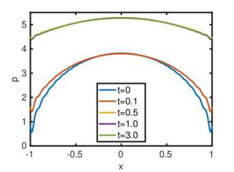
We verify the approach presented in Section 4 by comparing the solution formula given in Theorem 6, with $d_{\perp}\left(t\right)\equiv 0$, $d_{\perp}^{0}=l_{\perp}=0$ (according to Proposition 14), to a numerical finite-difference method for solving integral equation (4.24) in time. In particular, we truncate the series in (4.28) at $60$ terms (however, much less would already be sufficient). For the numerical approach, we combine Nyström collocation method with a finite-difference scheme in time using singularity subtraction. In Figure 6.1, we see that both solutions almost coincide for all shown instances of time. The solutions have an oscillatory mismatch, especially in small regions close to the endpoints $x=\pm 1$, which is a typical phenomenon for a spectral approach.

Refer to caption
Refer to caption
Figure 6.1. Time evolution of the pressure profile computed from equation (4.27) (left) and by a numerical finite-difference method (right)

6.2. Dependence of the stationary state on the model parameter $\mu$

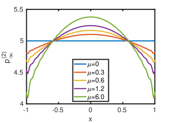
Let us consider the same setup as in Subsection 6.1, but instead of a fixed value of $\mu$, we explore the range of this model parameter starting from the degenerate case $\mu=0$ (purely fractional order model for the wear term (2.4) given by (3.6)) up to $\mu=6$. This is done in order to investigate the effect of such a parameter variation on an essential output of the model: the stationary pressure distribution $p_{\infty}^{\left(2\right)}\left(x\right)$ given by (5.10). As Figure 6.2 shows, the increase of $\mu$ amounts to steepening of the curve $p_{\infty}^{\left(2\right)}\left(x\right)$ making a deviation from the uniform pressure distribution more pronounced. Note that, according to (5.10), the stationary pressure distribution is independent of the model parameter $\alpha$.

Refer to caption
Figure 6.2. Effect of the model parameter $\mu$ on the stationary state $p_{\infty}^{\left(2\right)}\left(x\right)$

6.3. Illustration of the convergence under a constant load

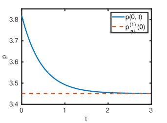
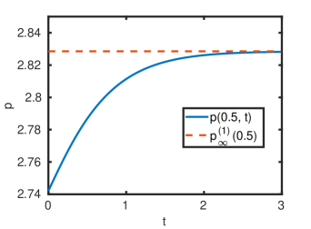
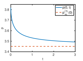
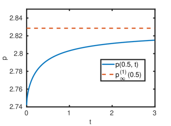
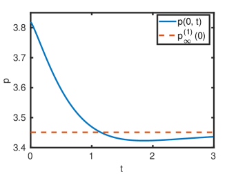
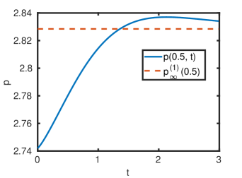
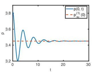
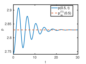
We now consider a simple setting which is more classical for analysis: the constant load case, i.e. we replace (6.1) with $P\left(t\right)\equiv P_{0}$, $t\geq 0$. We take (6.2) and numerical values of $P_{0}$ and other parameters as in Subsection 6.1, except for the model “order” parameter $\alpha$ which we now vary. The goal here is to demonstrate qualitatively different behaviour of the model depending on this parameter. In particular, we investigate three different values of $\alpha$, by looking at the pressure evolution at two particular points. For $\alpha=1$, the convergence to the stationary value occurs fast, and hence Figure 6.3 corroborates exponential bound (5.1). For all other values of $\alpha$ inside the interval $\left(0,2\right)$, the stabilisation occurs only at an algebraic rate. In particular, this is illustrated in Figures 6.4 and 6.5 where values $\alpha=0.6$ and $\alpha=1.2$ are taken, respectively. We see that in the first case convergence happens monotonically whereas in the second one it is accompanied by oscillations. Figure 6.6 shows, on extended time interval, that for a larger value ($\alpha=1.8$), oscillations increase even more.

Refer to caption
Refer to caption
Figure 6.3. $\alpha=1$: Time evolution of the pressure at $x=0$ (left) and $x=0.5$ (right)
Refer to caption
Refer to caption
Figure 6.4. $\alpha=0.6$: Time evolution of the pressure at $x=0$ (left) and $x=0.5$ (right)
Refer to caption
Refer to caption
Figure 6.5. $\alpha=1.2$: Time evolution of the pressure at $x=0$ (left) and $x=0.5$ (right)
Refer to caption
Refer to caption
Figure 6.6. $\alpha=1.8$: Time evolution of the pressure at $x=0$ (left) and $x=0.5$ (right)

7. Discussion and conclusion

Several formulations of the punch-sliding problem have been considered at once. These included rather general relation between contact pressure and displacement generalising the half-space geometry, a potential presence of coating (or additional surface microstructure), time-varying load and a linear material wear. In particular, the wear was modelled through a novel non-local relation between the contact pressure and the wear generalising the classical one. One advantage of transient models with such a wear relation is that they admit a closed-form solution as long as the spatial part of the formulation can be easily resolved and, most importantly, analysed. This possibility should not be underestimated in contexts of inverse design of mechanical materials.

Another relevant advantage is that the solution may exhibit predictably different transient behavior and the stationary pressure distribution depending on newly introduced parameters entering the formulation. As it was shown numerically, these parameters can be chosen to ensure a slow algebraic stabilisation towards the stationary distribution whether its monotone or oscillatory. This complements the fast exponential stabilisation (which happens in the particular case of the model parameter $\alpha=1$), a typically occuring phenomenon for such problems, and paves a way for description of new materials such as polymers within the same framework.

The non-uniform stationary pressure distributions are also possible and correspond to non-zero values of the model parameter $\mu$. At the next stage, a practical validation of the obtained results and a fit of the model to experimental data is highly desirable. In doing this, the parameter $\mu$ should be chosen from an observation of the stationary pressure distribution whereas the parameter $\alpha$ should be determined from temporal observations (the convergence speed), according to what was described above.

We thus conclude that the proposed model has a potential to describe materials whose temporal convergence to a stationary state is slow as well as those for which the stationary pressure distribution is not uniform.

As a continuation of this work, analysis of the long-time behavior under a periodic load $P$ has already been considered in [31]. More challenging would be to deal rigorously with more general kernel functions $K$ such as those that do not satisfy the parity assumption. However, it seems that the positivity assumption is not essential, and, in view of that, some technical results in Appendix are already provided for a slightly more general setting than the one being considered here.

Acknowledgements

The author is grateful for the support of the bi-national FWF-project I3538-N32 of the Austrian Science Fund (FWF) used for his employment at Vienna University of Technology. The paper has benefited from fruitful discussions with Ivan Argatov on mechanical aspects of the matter.

Appendix A

We collect here some auxiliary results that are needed in the paper.

A.1. Basic theoretical facts about compact linear integral operators

Lemma 17.

Let $K\in L^{2}\left(\left(-a,a\right)\times\left(-a,a\right)\right)$, i.e. such that

(A.1) $$\int_{-a}^{a}\int_{-a}^{a}\left[K\left(x,\xi\right)\right]^{2}\mathrm{d}x\mathrm{d}\xi<\infty.$$

Then, the integral transformation $f\mapsto\mathfrak{K}\left[f\right]\left(x\right):=\int_{-a}^{a}K\left(x,\xi\right)f\left(\xi\right)\mathrm{d}\xi$ is a compact linear operator from $L^{2}\left(-a,a\right)$ to $L^{2}\left(-a,a\right)$.

Proof.

Under assumption of the validity of (A.1), it follows that $\mathfrak{K}\left[f\right]\in L^{2}\left(-a,a\right)$ by an application of the Cauchy-Schwarz inequality (see also [22, Lem 3.2.3]). The fact that the operator $\mathfrak{K}$ is compact can be shown [22, Thm 3.2.7] using Weierstrass approximation theorem and the characterisation of a compact operator as the limit of finite rank operators. ∎

Lemma 18.

Let $X$ be a Hilbert space and $\mathcal{A}:\,X\rightarrow X$ be a compact self-adjoint operator. Then, the eigenvalues of $\mathcal{A}$ form a real non-increasing in absolute value sequence, and every eigenvalue different from zero has finite multiplicity. Moreover, the eigenfunctions of $\mathcal{A}$ form an orthonormal basis in $\overline{\text{Ran }\mathcal{A}}$, the closure of the range of $\mathcal{A}$.

Proof.

The statement of the lemma is a collection of standard results of the spectral theory of compact self-adjoint operators. A close result in the form of a single theorem is given in [5, Thm 2.8.15]. See also [35, Sect. 97 Thm p.242] and [38, Thm 5.6]. ∎

Lemma 19.

[35, Sect. 95 Thm p. 237] Let $X$ be a Hilbert space with the inner product $\left\langle\cdot,\cdot\right\rangle_{X}$, and $\mathcal{A}:\,X\rightarrow X$ is a compact self-adjoint operator. Then, $\lambda_{n}^{+}$, the $n$-th largest positive eigenvalue of $\mathcal{A}$ can be characterised as

$$\lambda_{1}^{+}=\max_{\begin{subarray}{c}f\in X\end{subarray}}\frac{\left\langle\mathcal{A}\left[f\right],f\right\rangle_{X}}{\left\langle f,f\right\rangle_{X}},\hskip 10.00002pt\hskip 10.00002pt\lambda_{n}^{+}=\max_{\begin{subarray}{c}f\in X\\ f\perp\left(\varphi_{1}^{+},\ldots\varphi_{n-1}^{+}\right)\end{subarray}}\frac{\left\langle\mathcal{A}\left[f\right],f\right\rangle_{X}}{\left\langle f,f\right\rangle_{X}},\hskip 10.00002ptn\geq 2,$$

where $\varphi_{1}^{+},\dots\varphi_{n-1}^{+}$ are the eigenfunctions corresponding to the $n-1$ largest positive eigenvalues, and the orthogonality condition $f\perp\left(\varphi_{1}^{+},\ldots\varphi_{n-1}^{+}\right)$ means that $\left\langle f,\varphi_{j}^{+}\right\rangle_{X}=0$, $j=1$, $\ldots$, $n-1$. Similarly, $\lambda_{n}^{-}$, the $n$-th smallest negative eigenvalue of $\mathcal{A}$ can be characterised as

$$\lambda_{1}^{-}=\min_{\begin{subarray}{c}f\in X\end{subarray}}\frac{\left\langle\mathcal{A}\left[f\right],f\right\rangle_{X}}{\left\langle f,f\right\rangle_{X}},\hskip 10.00002pt\hskip 10.00002pt\lambda_{n}^{-}=\min_{\begin{subarray}{c}f\in X\\ f\perp\left(\varphi_{1}^{-},\ldots\varphi_{n-1}^{-}\right)\end{subarray}}\frac{\left\langle\mathcal{A}\left[f\right],f\right\rangle_{X}}{\left\langle f,f\right\rangle_{X}},\hskip 10.00002ptn\geq 2,$$

where $\varphi_{1}^{-},\dots\varphi_{n-1}^{-}$ are the eigenfunctions corresponding to the $n-1$ smallest negative eigenvalues.

.

Lemma 20.

[35, Sect. 95 Thm p. 237] Let $X$ be a Hilbert space with the inner product $\left\langle\cdot,\cdot\right\rangle_{X}$, and $\mathcal{A}:\,X\rightarrow X$ is a compact self-adjoint operator. Then, $\lambda_{n}$, the $n$-th largest eigenvalue of $\mathcal{A}$ can be characterised as

$$\lambda_{n}=\min_{f_{1},\ldots,f_{n-1}\in X}\max_{\begin{subarray}{c}f\in X\\ f\perp\left(f_{1},\ldots f_{n-1}\right)\end{subarray}}\frac{\left\langle\mathcal{A}\left[f\right],f\right\rangle_{X}}{\left\langle f,f\right\rangle_{X}},\hskip 10.00002ptn\geq 2,$$

where the orthogonality condition $f\perp\left(f_{1},\ldots f_{n-1}\right)$ means that $\left\langle f,f_{j}\right\rangle_{X}=0$, $j=1$, $\ldots$, $n-1$.

A.2. Some special functions and their properties

abc

Gamma function:

(A.2) $$\Gamma\left(z\right):=\int_{0}^{\infty}x^{z-1}e^{-x}\mathrm{d}x,\hskip 10.00002ptz>0.$$

This function satisfies the following fundamental relation

(A.3) $$\Gamma\left(z+1\right)=z\Gamma\left(z\right),\hskip 10.00002pt\hskip 10.00002pt\Gamma\left(n+1\right)=n!,\hskip 10.00002ptz>0,\hskip 10.00002ptn\in\mathbb{N}_{0},$$

as well as Euler’s reflection formula

(A.4) $$\Gamma\left(1-z\right)\Gamma\left(z\right)=\frac{\pi}{\sin\left(\pi z\right)},\hskip 10.00002ptz\notin\mathbb{Z}.$$

Mittag-Leffler and relevant functions:

(A.5) $$E_{\alpha}\left(z\right):=\sum_{k=0}^{\infty}\frac{z^{k}}{\Gamma\left(\alpha k+1\right)},\hskip 10.00002pt\hskip 10.00002ptE_{\alpha,\beta}\left(z\right):=\sum_{k=0}^{\infty}\frac{z^{k}}{\Gamma\left(\alpha k+\beta\right)},\hskip 10.00002pt\hskip 10.00002ptz\in\mathbb{C},\hskip 10.00002pt\alpha,\,\beta>0,$$
(A.6) $$e_{\alpha}\left(z;\lambda\right):=\frac{\mathrm{d}}{\mathrm{d}z}E_{\alpha}\left(-\lambda z^{\alpha}\right)=\frac{\alpha}{z}\sum_{k=1}^{\infty}\frac{\left(-1\right)^{k}k\lambda^{k}z^{\alpha k}}{\Gamma\left(\alpha k+1\right)},\hskip 10.00002ptz>0,\hskip 10.00002pt\alpha>0,\hskip 10.00002pt\lambda\in\mathbb{C},$$
(A.7) $$\mathcal{E_{\alpha}}\left(z\right):=e_{\alpha}\left(z;1\right)=\frac{\alpha}{z}\sum_{k=1}^{\infty}\frac{\left(-1\right)^{k}kz^{\alpha k}}{\Gamma\left(\alpha k+1\right)},\hskip 10.00002ptz>0,\hskip 10.00002pt\alpha>0.$$

The following two identities are direct consequences of definitions (A.5) and (A.3)

(A.8) $$E_{\alpha,1}\left(z\right)=E_{\alpha}\left(z\right),\hskip 10.00002pt\hskip 10.00002ptE_{1}\left(z\right)=\exp\left(z\right),\hskip 10.00002ptz\in\mathbb{C}.$$

Note that when $\lambda>0$, we can write

(A.9) $$e_{\alpha}\left(z;\lambda\right)=\lambda^{1/\alpha}\mathcal{E_{\alpha}}\left(\lambda^{1/\alpha}z\right),\hskip 10.00002ptz>0,\hskip 10.00002pt\alpha>0,\hskip 10.00002pt\lambda>0.$$

We have a useful relation

(A.10) $$E_{\alpha,\alpha}\left(z\right)=\alpha E_{\alpha,1}^{\prime}\left(z\right)=\alpha E_{\alpha}^{\prime}\left(z\right),\hskip 10.00002ptz\in\mathbb{C},\hskip 10.00002pt\alpha>0,$$

which is straightforward to obtain using definitions (A.5) and (A.3). Also, from (A.9) and (A.6), it follows that

(A.11) $$\int_{0}^{z_{0}}\mathcal{E}_{\alpha}\left(\lambda^{1/\alpha}z\right)\mathrm{d}z=\lambda^{-1/\alpha}\int_{0}^{z_{0}}e_{\alpha}\left(z;\lambda\right)\mathrm{d}z=\lambda^{-1/\alpha}\left[E_{\alpha}\left(-\lambda z_{0}^{\alpha}\right)-1\right],\hskip 10.00002ptz_{0}>0,\hskip 10.00002pt\alpha>0,\hskip 10.00002pt\lambda>0.$$

Moreover, when $\alpha\in\left(0,1\right)$, we have the following integral representation

(A.12) $$\mathcal{E}_{\alpha}\left(z\right)=-\frac{\sin\left(\alpha\pi\right)}{\pi}{\displaystyle\int_{0}^{\infty}}e^{-rz}\frac{r^{\alpha}}{r^{2\alpha}+2r^{\alpha}\cos\left(\alpha\pi\right)+1}\mathrm{d}r,\hskip 10.00002pt0<\alpha<1,\hskip 10.00002ptz>0,$$

which can be obtained from [20, eqs. (3.19)–(3.20), (3.24)–(3.25)] by differentiation.

Small-argument asymptotics of the above functions follow directly from definitions (A.5)–(A.7)

(A.13) $$E_{\alpha}\left(z\right)=1+\frac{z}{\Gamma\left(1+\alpha\right)}+\mathcal{O}\left(z^{2}\right),\hskip 10.00002pt\hskip 10.00002pte_{\alpha}\left(z;\lambda\right)=-\frac{\alpha\lambda}{\Gamma\left(1+\alpha\right)}\frac{1}{z^{1-\alpha}}+\mathcal{O}\left(\frac{1}{z^{1-2\alpha}}\right),\hskip 10.00002pt\hskip 10.00002pt\left|z\right|\ll 1,$$
(A.14) $$\mathcal{E_{\alpha}}\left(z\right)=-\frac{\alpha}{\Gamma\left(1+\alpha\right)}\frac{1}{z^{1-\alpha}}+\mathcal{O}\left(\frac{1}{z^{1-2\alpha}}\right),\hskip 10.00002pt\hskip 10.00002pt\left|z\right|\ll 1.$$

Large-argument asymptotics of $\mathcal{E}_{\alpha}\left(z;\lambda\right)$ can be derived from that of $E_{\alpha}\left(z\right)$ given, for example, in [19, eqs. (3.4.14)–(3.4.15)] (see also [29, eq. (1.2)] for the same results for $\alpha\in\left(0,1\right)$)

(A.15) $$E_{\alpha}\left(z\right)=\frac{1}{\alpha}\exp\left(z^{1/\alpha}\right)-\sum_{k=1}^{\infty}\frac{z^{-k}}{\Gamma\left(1-\alpha k\right)},\hskip 10.00002pt\hskip 10.00002ptE_{\alpha}\left(-z\right)=-\sum_{k=1}^{\infty}\frac{\left(-1\right)^{k}z^{-k}}{\Gamma\left(1-\alpha k\right)},\hskip 10.00002pt\hskip 10.00002ptz\gg 1,\hskip 10.00002pt\alpha\in\left(0,1\right)\cup\left(1,2\right),$$
(A.16) $$e_{\alpha}\left(z;\lambda\right)=\begin{cases}-\frac{\alpha}{\lambda\Gamma\left(1-\alpha\right)}\frac{1}{z^{\alpha+1}}+\mathcal{O}\left(\frac{1}{z^{2\alpha+1}}\right),&z\gg 1,\hskip 10.00002pt\lambda>0,\hskip 10.00002pt\alpha\in\left(0,1\right)\cup\left(1,2\right),\\ \frac{\lambda^{1/\alpha}}{\alpha}\exp\left(\lambda^{1/\alpha}z\right)+\frac{\alpha}{\lambda\Gamma\left(1-\alpha\right)}\frac{1}{z^{\alpha+1}}+\mathcal{O}\left(\frac{1}{z^{2\alpha+1}}\right),&z\gg 1,\hskip 10.00002pt\lambda<0,\hskip 10.00002pt\alpha\in\left(0,1\right)\cup\left(1,2\right),\end{cases}$$
(A.17) $$\mathcal{E_{\alpha}}\left(z\right)=-\frac{\alpha}{\Gamma\left(1-\alpha\right)}\frac{1}{z^{\alpha+1}}+\mathcal{O}\left(\frac{1}{z^{2\alpha+1}}\right),\hskip 10.00002pt\hskip 10.00002ptz\gg 1,\hskip 10.00002pt\alpha\in\left(0,1\right)\cup\left(1,2\right).$$

We also need some Laplace transforms of the above functions. We denote the Laplace transform of $f$ as $\mathcal{L}\left[f\right]\left(s\right):=\int_{0}^{\infty}f\left(t\right)e^{-st}\mathrm{d}t$. In particular, we have (see [20, eq. (3.14)] or [27, eq. (4)])

(A.18) $$\mathcal{L}\left[\mathcal{E}_{\alpha}\right]\left(s\right)=-\frac{1}{s^{\alpha}+1},\hskip 10.00002pt\alpha>0,$$

which implies that, for $\lambda>0$,

(A.19) $$\mathcal{L}^{-1}\left[\frac{1}{s^{\alpha}+\lambda}\right]\left(t\right)=-\frac{1}{\lambda^{1-1/\alpha}}\mathcal{E}_{\alpha}\left(\lambda^{1/\alpha}t\right)=-\frac{1}{\lambda}e_{\alpha}\left(t;\lambda\right),\hskip 10.00002pt\alpha>0.$$

To obtain similar result for $\lambda<0$, we use the formula [36, eq. (1.93)]

$$\mathcal{L}\left[\frac{1}{t^{1-\alpha}}E_{\alpha,\alpha}\left(t^{\alpha}\right)\right]\left(s\right)=\frac{1}{s^{\alpha}-1},\hskip 10.00002pt\text{Re }s>1,\hskip 10.00002pt\alpha>0,$$

which implies that

(A.20) $\displaystyle\mathcal{L}^{-1}\left[\frac{1}{s^{\alpha}-\left|\lambda\right|}\right]\left(t\right)=$ $\displaystyle\frac{1}{t^{1-\alpha}}E_{\alpha,\alpha}\left(\left|\lambda\right|t^{\alpha}\right)=\frac{\alpha}{t^{1-\alpha}}E_{\alpha}^{\prime}\left(\left|\lambda\right|t^{\alpha}\right)=\frac{1}{\left|\lambda\right|}\frac{\mathrm{d}}{\mathrm{d}t}E_{\alpha}\left(\left|\lambda\right|t^{\alpha}\right)$
$\displaystyle=$ $\displaystyle-\frac{1}{\lambda}\frac{\mathrm{d}}{\mathrm{d}t}E_{\alpha}\left(-\lambda t^{\alpha}\right)=-\frac{1}{\lambda}e_{\alpha}\left(t;\lambda\right).$

Here, we used the identity (A.10) and the definition of the function $\mathcal{E}_{a}$.
Note that (A.20) shows that (A.19) is actually valid for all $\lambda\in\mathbb{R}$.

A.3. Some singular integral equations and their solutions

We consider here Abel’s integral equations of the first and the second kinds and two other related equations.

Lemma 21.

[19, Thm 4.2] Let $\alpha>0$, $\lambda\in\mathbb{C}$ and $f\in L^{1}\left(0,T\right)$ for any $T>0$. Then, the integral equation

(A.21) $$u\left(t\right)+\frac{\lambda}{\Gamma\left(\alpha\right)}\int_{0}^{t}\frac{u\left(\tau\right)}{\left(t-\tau\right)^{1-\alpha}}\mathrm{d}\tau=f\left(t\right),\hskip 10.00002ptt\in\left(0,T\right),$$

has a unique solution $u\in L^{1}\left(0,T\right)$ given by

(A.22) $\displaystyle u\left(t\right)=$ $\displaystyle f\left(t\right)-\lambda\int_{0}^{t}\frac{E_{\alpha,\alpha}\left(-\lambda\left(t-\tau\right)^{\alpha}\right)}{\left(t-\tau\right)^{1-\alpha}}f\left(\tau\right)\mathrm{d}\tau$
$\displaystyle=$ $\displaystyle f\left(t\right)+\int_{0}^{t}e_{\alpha}\left(t-\tau;\lambda\right)f\left(\tau\right)\mathrm{d}\tau,\hskip 10.00002ptt\in\left(0,T\right).$

Note that the integral form of the solution on the second line of (A.22) can be seen due to the identity (A.10), and it is also given elsewhere (see [19, eq. (8.1.20)], [20, eq. (2.12)]).

Lemma 22.

[36, Thm 2.1 & Lem. 2.1] (see also [19, Sect. 8.1.1]) Let $\alpha\in\left(0,1\right)$, and assume that $f$ is such that $\int_{0}^{t}\frac{f\left(\tau\right)}{\left(t-\tau\right)^{\alpha}}\mathrm{d}\tau$ is an absolutely continuous function on $\left[0,T\right]$ for some $T>0$ and, moreover, ${\displaystyle\lim_{t\rightarrow 0^{+}}}\int_{0}^{t}\frac{f\left(\tau\right)}{\left(t-\tau\right)^{\alpha}}\mathrm{d}\tau=0$. Then, the integral equation

(A.23) $$\frac{1}{\Gamma\left(\alpha\right)}\int_{0}^{t}\frac{u\left(\tau\right)}{\left(t-\tau\right)^{1-\alpha}}\mathrm{d}\tau=f\left(t\right),\hskip 10.00002ptt\in\left(0,T\right),$$

has a unique solution $u\in L^{1}\left(0,T\right)$ given by

(A.24) $$u\left(t\right)=\frac{1}{\Gamma\left(1-\alpha\right)}\frac{\mathrm{d}}{\mathrm{d}t}\int_{0}^{t}\frac{f\left(\tau\right)}{\left(t-\tau\right)^{\alpha}}\mathrm{d}\tau,\hskip 10.00002ptt\in\left(0,T\right).$$

In particular, to satisfy the aforementioned conditions on $f$, it is sufficient that $f$ is an absolutely continuous function on $\left[0,T\right]$. In this case, the solution (A.24) can be written in the alternative form

(A.25) $$u\left(t\right)=\frac{1}{\Gamma\left(1-\alpha\right)}\left[\frac{f\left(0\right)}{t^{\alpha}}+\int_{0}^{t}\frac{f^{\prime}\left(\tau\right)}{\left(t-\tau\right)^{\alpha}}\mathrm{d}\tau\right],\hskip 10.00002ptt\in\left(0,T\right).$$

.

Corollary 23.

Let $\alpha\in\left[1,2\right)$, and assume that $f$ is such that $\int_{0}^{t}\frac{f\left(\tau\right)}{\left(t-\tau\right)^{\alpha-1}}\mathrm{d}\tau$ is an absolutely continuous function on $\left[0,T\right]$ for some $T>0$ and, moreover, ${\displaystyle\lim_{t\rightarrow 0^{+}}}\int_{0}^{t}\frac{f\left(\tau\right)}{\left(t-\tau\right)^{\alpha-1}}\mathrm{d}\tau=0$. Then, integral equation (A.23) has a unique solution $u$ such that $\int_{0}^{\cdot}u\left(\tau\right)\mathrm{d}\tau\in L^{1}\left(0,T\right)$ and it is given by

(A.26) $$u\left(t\right)=\frac{\Gamma\left(\alpha\right)\sin\left[\pi\left(\alpha-1\right)\right]}{\pi\left(\alpha-1\right)}\frac{\mathrm{d}^{2}}{\mathrm{d}t^{2}}\int_{0}^{t}\frac{f\left(\tau\right)}{\left(t-\tau\right)^{\alpha-1}}\mathrm{d}\tau,\hskip 10.00002ptt\in\left(0,T\right).$$

Moreover, if $f^{\prime}$ is absolutely continuous on $\left[0,T\right]$, solution formula (A.26) can be rewritten as

(A.27) $$u\left(t\right)=\frac{\Gamma\left(\alpha\right)\sin\left[\pi\left(\alpha-1\right)\right]}{\pi\left(\alpha-1\right)}\left[-\frac{\alpha-1}{t^{\alpha}}f\left(0\right)+\frac{f^{\prime}\left(0\right)}{t^{\alpha-1}}+\int_{0}^{t}\frac{f^{\prime\prime}\left(\tau\right)}{\left(t-\tau\right)^{\alpha-1}}\mathrm{d}\tau\right],\hskip 10.00002ptt\in\left(0,T\right).$$
Proof.

Let us first assume that $\alpha\in\left(1,2\right)$. Denoting $\widetilde{u}\left(t\right):=\int_{0}^{t}u\left(\tau\right)\mathrm{d}\tau$, integration by parts yields

$$\int_{0}^{t}\frac{u\left(\tau\right)}{\left(t-\tau\right)^{1-\alpha}}\mathrm{d}\tau=\left(\alpha-1\right)\int_{0}^{t}\frac{\widetilde{u}\left(\tau\right)}{\left(t-\tau\right)^{2-\alpha}}\mathrm{d}\tau,$$

where the boundary terms vanish due to $\alpha>1$ and $\widetilde{u}\left(0\right)=0$. Lemma 22 now applies to the equation

$$\frac{1}{\Gamma\left(\alpha-1\right)}\int_{0}^{t}\frac{\widetilde{u}\left(\tau\right)}{\left(t-\tau\right)^{2-\alpha}}\mathrm{d}\tau=\frac{\Gamma\left(\alpha\right)}{\left(\alpha-1\right)\Gamma\left(\alpha-1\right)}f\left(t\right),\hskip 10.00002ptt\in\left(0,T\right),$$

and gives the existence of a unique solution $\tilde{u}\in L^{1}\left(0,T\right)$:

(A.28) $$\widetilde{u}\left(t\right)=\frac{\Gamma\left(\alpha\right)}{\left(\alpha-1\right)\Gamma\left(\alpha-1\right)\Gamma\left(2-\alpha\right)}\frac{\mathrm{d}}{\mathrm{d}t}\int_{0}^{t}\frac{f\left(\tau\right)}{\left(t-\tau\right)^{\alpha-1}}\mathrm{d}\tau,\hskip 10.00002ptt\in\left(0,T\right).$$

Hence, differentiating and using the identity $\Gamma\left(\alpha-1\right)\Gamma\left(2-\alpha\right)=\pi/\sin\left[\pi\left(\alpha-1\right)\right]$ (see (A.4)), we obtain (A.26).

Suppose now that $f$ is absolutely continuous on $\left[0,T\right]$, we can then integrate by parts, taking into account that $\alpha<2$,

(A.29) $\displaystyle\int_{0}^{t}\frac{f\left(\tau\right)}{\left(t-\tau\right)^{\alpha-1}}\mathrm{d}\tau=$ $\displaystyle\int_{0}^{t}\frac{f\left(t-\tau\right)}{\tau^{\alpha-1}}\mathrm{d}\tau=\frac{t^{2-\alpha}}{2-\alpha}f\left(0\right)+\frac{1}{2-\alpha}\int_{0}^{t}f^{\prime}\left(t-\tau\right)\tau^{2-\alpha}\mathrm{d}\tau$
$\displaystyle=$ $\displaystyle\frac{t^{2-\alpha}}{2-\alpha}f\left(0\right)+\frac{1}{2-\alpha}\int_{0}^{t}f^{\prime}\left(\tau\right)\left(t-\tau\right)^{2-\alpha}\mathrm{d}\tau,$

and thus

(A.30) $$\frac{\mathrm{d}}{\mathrm{d}t}\int_{0}^{t}\frac{f\left(\tau\right)}{\left(t-\tau\right)^{\alpha-1}}\mathrm{d}\tau=\frac{f\left(0\right)}{t^{\alpha-1}}+\int_{0}^{t}\frac{f^{\prime}\left(\tau\right)}{\left(t-\tau\right)^{\alpha-1}}\mathrm{d}\tau.$$

If $f^{\prime}$ is absolutely continuous on $\left[0,T\right]$, we can apply the same procedure to the integral on the right-hand side before another differentiation and then we arrive at

$$\frac{\mathrm{d}^{2}}{\mathrm{d}t^{2}}\int_{0}^{t}\frac{f\left(\tau\right)}{\left(t-\tau\right)^{\alpha-1}}\mathrm{d}\tau=-\frac{\alpha-1}{t^{\alpha}}f\left(0\right)+\frac{f^{\prime}\left(0\right)}{t^{\alpha-1}}+\int_{0}^{t}\frac{f^{\prime\prime}\left(\tau\right)}{\left(t-\tau\right)^{\alpha-1}}\mathrm{d}\tau,$$

which, upon insertion into (A.26), gives (A.27).

Now, we consider the situation when $\alpha=1$. Equation (A.23) degenerates and its unique solution $u\left(t\right)=f^{\prime}\left(t\right)$ follows immediately by differentiation of both sides of the equation. Taking into account that $\frac{\sin\left[\pi\left(\alpha-1\right)\right]}{\pi\left(\alpha-1\right)}\rightarrow 1$ as $\alpha\rightarrow 1$, upon an elementary simplification, we see that this solution coincides precisely with (A.27) for $\alpha=1$. ∎

Lemma 24.

Let $\alpha>0$, $\lambda\in\mathbb{R}$. Then, the integral equation

(A.31) $$u\left(t\right)-\lambda\int_{0}^{t}\mathcal{E}_{\alpha}\left(t-\tau\right)u\left(\tau\right)\mathrm{d}\tau=f\left(t\right),\hskip 10.00002ptt>0,$$

has a unique solution given by

(A.32) $$u\left(t\right)=f\left(t\right)+\frac{\lambda}{1+\lambda}\int_{0}^{t}e_{\alpha}\left(t-\tau;1+\lambda\right)f\left(\tau\right)\mathrm{d}\tau,\hskip 10.00002ptt>0.$$
Proof.

Let us denote $U\left(s\right):=\mathcal{L}\left[u\right]\left(s\right)$, $F\left(s\right):=\mathcal{L}\left[f\right]\left(s\right)$ the Laplace transforms of $u\left(t\right)$ and $f\left(t\right)$, respectively. Application of the Laplace transformation to the both sides of (A.31) yields, upon using the convolution theorem and (A.18),

(A.33) $$U\left(s\right)+\frac{\lambda}{s^{\alpha}+1}U\left(s\right)=F\left(s\right)\hskip 10.00002pt\Longrightarrow\hskip 10.00002ptU\left(s\right)=\frac{s^{\alpha}+1}{s^{\alpha}+1+\lambda}F\left(s\right)=\left[1-\frac{\lambda}{s^{\alpha}+1+\lambda}\right]F\left(s\right).$$

Using (A.19), inversion of Laplace transformation of the rightmost equation above leads to (A.32). ∎

Corollary 25.

Let $\alpha>0$, $\mu\geq 0$, $\lambda\in\mathbb{R}$. Then, the integral equation

(A.34) $$u\left(t\right)-\frac{\lambda}{\mu^{1-1/\alpha}}\int_{0}^{t}\mathcal{E}_{\alpha}\left(\mu^{1/\alpha}\left(t-\tau\right)\right)u\left(\tau\right)\mathrm{d}\tau=f\left(t\right),\hskip 10.00002ptt>0,$$

has a unique solution given by

(A.35) $\displaystyle u\left(t\right)$ $\displaystyle=f\left(t\right)+\frac{\lambda}{\mu+\lambda}\int_{0}^{t}e_{\alpha}\left(t-\tau;\mu+\lambda\right)f\left(\tau\right)\mathrm{d}\tau$
$\displaystyle=f\left(t\right)+\frac{\lambda}{\left(\mu+\lambda\right)^{1-1/\alpha}}\int_{0}^{t}\mathcal{E}_{\alpha}\left(\left(\mu+\lambda\right)^{1/\alpha}\left(t-\tau\right)\right)f\left(\tau\right)\mathrm{d}\tau,\hskip 10.00002ptt>0.$
Proof.

For $\mu>0$, the result follows from Lemma 24 applied to the integral equation for $u\left(t/\mu^{1/\alpha}\right)$ with $\lambda/\mu$ and $f\left(t/\mu^{1/\alpha}\right)$ in place of $\lambda$ and $f\left(t\right)$, respectively.

To treat the case $\mu=0$, we observe, using (A.14) and (A.3), that in the limit $\mu\rightarrow 0$, equation (A.34) becomes (A.21) whose solution, given by Lemma 21, coincides exactly with (A.35) for $\mu=0$. ∎

Lemma 26.

Let $\alpha\in\left(0,1\right)$, and assume that $f$ is an absolutely continuous function on every subinterval of $\mathbb{R}_{+}$. Then, the integral equation

(A.36) $$\int_{0}^{t}\mathcal{E}_{\alpha}\left(t-\tau\right)u\left(\tau\right)\mathrm{d}\tau=f\left(t\right),\hskip 10.00002ptt>0,$$

has a unique solution given by

(A.37) $\displaystyle u\left(t\right)$ $\displaystyle=-\frac{f\left(0\right)}{\Gamma\left(1-\alpha\right)t^{\alpha}}-\int_{0}^{t}\left(1+\frac{1}{\Gamma\left(1-\alpha\right)}\frac{1}{\left(t-\tau\right)^{\alpha}}\right)f^{\prime}\left(\tau\right)\mathrm{d}\tau$
$\displaystyle=-f\left(t\right)-\text{$\left(\frac{1}{\Gamma\left(1-\alpha\right)t^{\alpha}}-1\right)$}f\left(0\right)-\frac{1}{\Gamma\left(1-\alpha\right)}\int_{0}^{t}\frac{f^{\prime}\left(\tau\right)}{\left(t-\tau\right)^{\alpha}}\mathrm{d}\tau,\hskip 10.00002ptt>0.$
Proof.

The proof is ideologically similar to that of Lemma 24. Let us denote $U\left(s\right):=\mathcal{L}\left[u\right]\left(s\right)$, $F\left(s\right):=\mathcal{L}\left[f\right]\left(s\right)$ the Laplace transforms of $u\left(t\right)$ and $f\left(t\right)$. Upon Laplace transformation of (A.36), using the convolution theorem and (A.18), we have

$$-U\left(s\right)\frac{1}{s^{\alpha}+1}=F\left(s\right)\hskip 10.00002pt\Longrightarrow\hskip 10.00002ptU\left(s\right)=-F\left(s\right)\left(1+s^{\alpha}\right)=-\left[sF\left(s\right)-f\left(0\right)\right]\left(\frac{1}{s}+\frac{1}{s^{1-\alpha}}\right)-f\left(0\right)\left(\frac{1}{s}+\frac{1}{s^{1-\alpha}}\right).$$

Hence, employing $\mathcal{L}\left[t^{\beta-1}\right]\left(s\right)=\Gamma\left(\beta\right)/s^{\beta}$, $\beta>0$ (see e.g. [13, pp. 318–319]), and, in particular, $\mathcal{L}\left[1\right]\left(s\right)=1/s$, we invert the transform to obtain (A.37). ∎

Corollary 27.

Let $\alpha\in\left(0,1\right)$, $\mu\geq 0$ and assume that $f$ is an absolutely continuous function on every bounded subinterval of $\mathbb{R}_{+}$. Then, the integral equation

(A.38) $$-\frac{1}{\mu^{1-1/\alpha}}\int_{0}^{t}\mathcal{E}_{\alpha}\left(\mu^{1/\alpha}\left(t-\tau\right)\right)u\left(\tau\right)\mathrm{d}\tau=f\left(t\right),\hskip 10.00002ptt>0,$$

has a unique solution given by

(A.39) $\displaystyle u\left(t\right)$ $\displaystyle=\frac{f\left(0\right)}{\Gamma\left(1-\alpha\right)t^{\alpha}}+\int_{0}^{t}\left(\mu+\frac{1}{\Gamma\left(1-\alpha\right)}\frac{1}{\left(t-\tau\right)^{\alpha}}\right)f^{\prime}\left(\tau\right)\mathrm{d}\tau$
$\displaystyle=\mu f\left(t\right)+\text{$\left(\frac{1}{\Gamma\left(1-\alpha\right)t^{\alpha}}-\mu\right)$}f\left(0\right)+\frac{1}{\Gamma\left(1-\alpha\right)}\int_{0}^{t}\frac{f^{\prime}\left(\tau\right)}{\left(t-\tau\right)^{\alpha}}\mathrm{d}\tau,\hskip 10.00002ptt>0.$
Proof.

For $\mu>0$, the result follows from Lemma 26 applied to the integral equation for $u\left(t/\mu^{1/\alpha}\right)$ with $-\mu f\left(t/\mu^{1/\alpha}\right)$ in place of $f\left(t\right)$.

To treat the case $\mu=0$, we observe, using (A.14) and (A.3), that in the limit $\mu\rightarrow 0$, equation (A.38) becomes (A.23) whose solution, given by Lemma 22, coincides exactly with (A.39) for $\mu=0$. ∎

Lemma 28.

Let $\alpha\in\left[1,2\right)$, $\mu\geq 0$, and assume that $f^{\prime}$ is an absolutely continuous function on every bounded subinterval of $\mathbb{R}_{+}$. Then, integral equation (A.38) has a unique solution given by

(A.40) $\displaystyle u\left(t\right)=\mu f\left(t\right)-\frac{\alpha-1}{\Gamma\left(2-\alpha\right)t^{\alpha}}f\left(0\right)+\frac{1}{\Gamma\left(2-\alpha\right)t^{\alpha-1}}f^{\prime}\left(0\right)+\frac{1}{\Gamma\left(2-\alpha\right)}\int_{0}^{t}\frac{f^{\prime\prime}\left(\tau\right)}{\left(t-\tau\right)^{\alpha-1}}\mathrm{d}\tau,\hskip 10.00002ptt>0.$
Proof.

Case $\mu>0$:

First, let us consider $\alpha\in\left(1,2\right)$. Let $\widetilde{u}\left(t\right):=\int_{0}^{t}u\left(\tau\right)\mathrm{d}\tau$. Since $\mathcal{E}_{\alpha}\left(0\right)=0$ for $\alpha>1$ and $\widetilde{u}\left(0\right)=0$, integration by parts of (A.38) leads to

$$-\frac{1}{\mu^{1-2/\alpha}}\int_{0}^{t}\mathcal{E}_{\alpha}^{\prime}\left(\mu^{1/\alpha}\left(t-\tau\right)\right)\widetilde{u}\left(\tau\right)\mathrm{d}\tau=f\left(t\right),\hskip 10.00002ptt>0.$$

Denoting $\widetilde{U}\left(s\right):=\mathcal{L}\left[\widetilde{u}\right]\left(s\right)$, $F\left(s\right):=\mathcal{L}\left[f\right]\left(s\right)$ the Laplace transforms of $\widetilde{u}\left(t\right)$ and $f\left(t\right)$, respectively, we apply Laplace transformation to the above equation and use the convolution theorem and $\mathcal{L}\left[\mathcal{E}_{\alpha}^{\prime}\left(\mu^{1/\alpha}\cdot\right)\right]$ $\left(s\right)=-\frac{\mu^{1-2/\alpha}s}{s^{\alpha}+\mu}$ (which easily follows from (A.18)) to arrive at

$$\widetilde{U}\left(s\right)\frac{s}{s^{\alpha}+\mu}=F\left(s\right)\hskip 10.00002pt\Longrightarrow\hskip 10.00002pt\widetilde{U}\left(s\right)=F\left(s\right)\left(\frac{\mu}{s}+s^{\alpha-1}\right)=\left[sF\left(s\right)-f\left(0\right)\right]\left(\frac{\mu}{s^{2}}+\frac{1}{s^{2-\alpha}}\right)+f\left(0\right)\left(\frac{\mu}{s^{2}}+\frac{1}{s^{2-\alpha}}\right).$$

Therefore, upon inversion of Laplace transformation, using that $\mathcal{L}\left[t^{1-\alpha}\right]\left(s\right)=\Gamma\left(2-\alpha\right)/s^{2-\alpha}$, $\alpha<2$, (and, in particular, $\mathcal{L}\left[t\right]\left(s\right)=1/s^{2}$), we obtain

(A.41) $$\widetilde{u}\left(t\right)=\int_{0}^{t}f^{\prime}\left(\tau\right)\left[\mu\left(t-\tau\right)+\frac{1}{\Gamma\left(2-\alpha\right)\left(t-\tau\right)^{\alpha-1}}\right]\mathrm{d}\tau+f\left(0\right)\left(\mu t+\frac{1}{\Gamma\left(2-\alpha\right)t^{\alpha-1}}\right),\hskip 10.00002ptt>0.$$

Note that, similarly to (A.29)–(A.30), we have, for $\alpha\in\left(1,2\right)$,

$$\int_{0}^{t}\frac{f^{\prime}\left(\tau\right)}{\left(t-\tau\right)^{\alpha-1}}\mathrm{d}\tau=\frac{t^{2-\alpha}}{2-\alpha}f^{\prime}\left(0\right)+\frac{1}{2-\alpha}\int_{0}^{t}f^{\prime\prime}\left(\tau\right)\left(t-\tau\right)^{2-\alpha}\mathrm{d}\tau,$$
$$\frac{\mathrm{d}}{\mathrm{d}t}\int_{0}^{t}\frac{f^{\prime}\left(\tau\right)}{\left(t-\tau\right)^{\alpha-1}}\mathrm{d}\tau=\frac{1}{t^{\alpha-1}}f^{\prime}\left(0\right)+\int_{0}^{t}\frac{f^{\prime\prime}\left(\tau\right)}{\left(t-\tau\right)^{\alpha-1}}\mathrm{d}\tau,$$

and hence, by differentiation of (A.41), we deduce (A.40).

It remains to consider the situation when $\alpha=1$. To this effect, we recall (A.9) and (A.6) which imply that $\mathcal{E}_{1}\left(\mu t\right)=-e^{-\mu t}$, and hence equation (A.38) can be recast as

$$\int_{0}^{t}e^{\mu\tau}u\left(\tau\right)\mathrm{d}\tau=e^{\mu t}f\left(t\right),\hskip 10.00002ptt>0,$$

which is then immediately solved by the differentiation to give $u\left(t\right)=\mu f\left(t\right)+f^{\prime}\left(t\right)$. This solution coincides with that given by (A.40), upon substitution $\alpha=1$ and relevant simplifications (integration and cancellations).

Case $\mu=0$:

Recalling (A.14) and (A.3), we observe that in the limit $\mu\rightarrow 0$, equation (A.38) becomes (A.23). Solution of the latter equation, for $\alpha\in\left[1,2\right)$, is given by Corollary 23. Using the identities $\Gamma\left(\alpha-1\right)\Gamma\left(2-\alpha\right)=\pi/\sin\left[\pi\left(\alpha-1\right)\right]$ and $\Gamma\left(\alpha\right)=\left(\alpha-1\right)\Gamma\left(\alpha-1\right)$, this solution can be seen to coincide with (A.40) for $\mu=0$. ∎

Lemma 29.

Suppose that $f\in C^{2}\left(\left[-a,a\right]\right)$, then, if $a\neq 2$, the integral equation

$$-\int_{-a}^{a}\log\left|x-\xi\right|u\left(\xi\right)\mathrm{d}\xi=f\left(x\right),\hskip 10.00002ptx\in\left(-a,a\right),$$

admits a solution given by

$$u\left(x\right)=-\frac{1}{\left(a^{2}-x^{2}\right)^{1/2}}\left[\fint_{-a}^{a}\frac{\left(a^{2}-\xi^{2}\right)^{1/2}f^{\prime}\left(\xi\right)}{\xi-x}\mathrm{d}\xi+\frac{1}{\log\left(a/2\right)}\int_{-a}^{a}\frac{f\left(\xi\right)}{\left(a^{2}-\xi^{2}\right)^{1/2}}\mathrm{d}\xi\right],\hskip 10.00002ptx\in\left(-a,a\right).$$

Moreover, this solution is unique in the class of Hölder continuous functions with possible integrable singularities at the endpoints of the interval $\left[-a,a\right]$.

Proof.

See e.g. [12, p. 428] for the case $a=1$ and [16, p. 591] for arbitrary $a>0$, $a\neq 2$. ∎

References

  • [1] Alblas, J. B., Kuipers, M.: Contact problems of a rectangular block on an elastic layer of finite thickness: the thin layer. Acta Mech., 8 (3), 133–145 (1969).
  • [2] Alblas, J. B., Kuipers, M.: Contact problems of a rectangular block on an elastic layer of finite thickness: the thick layer. Acta Mech., 9 (1), 1–12 (1970).
  • [3] Aleksandrov, V. M., Kovalenko, E. V.: Mathematical methods in problems with wear (in Russian). Nonlinear Models and Problems of Mechanics of Solids, Contributions edited by K. V. Frolov (1984).
  • [4] Aleksandrov, V. M., Kovalenko, E. V.: On the theory of contact problems in the presence of nonlinear wear (in Russian). Mech. Solids. 4, 98–108 (1982).
  • [5] Atkinson, K., Han, W.: Theoretical Numerical Analysis - A Functional Analysis Framework (3rd Ed.), Springer (2009).
  • [6] Archard, J. F.: Contact and Rubbing of Flat Surfaces. Journal of Applied Physics 24, 981 (1953).
  • [7] Argatov, I. I., Chai, Y. S.: Artificial neural network modeling of sliding wear. Proceedings of the Institution of Mechanical Engineers, Part J: Journal of Engineering Tribology, 235 (4), 748–757 (2021).
  • [8] Argatov, I. I., Chai, Y. S.: Contact Geometry Adaptation in Fretting Wear: A Constructive Review. Frontiers in Mechanical Engineering, 6 (2020).
  • [9] Argatov, I. I., Chai, Y. S.: Effective wear coefficient and wearing-in period for a functionally graded wear-resisting punch. Acta Mech. 230, 2295–2307 (2019).
  • [10] Argatov, I. I., Chai, Y. S.: Wear contact problem with friction: Steady-state regime and wearing-in period. Int. J. Sol. Struct. 193–194, 213–221 (2020).
  • [11] Argatov, I. I., Fadin, Yu. A.: A Macro-Scale Approximation for the Running-In Period. Tribol. Lett. 42, 311–317 (2011).
  • [12] Carrier, G. F., Krook, M., Pearson, C.E.: Functions of a complex variable: theory and technique. SIAM (2005).
  • [13] Doetsch, G.: Introduction to the Theory and Application of the Laplace Transformation. Springer-Verlag (1974).
  • [14] Dundurs, J., Comninou, M.: Shape of a worn slider. Wear, 62 (2), 419–424 (1980).
  • [15] Feppon, F., Sidebottom, M. A., Michailidis, G., Krick, B. A., Vermaak, N.: Efficient steady-state computation for wear of multimaterial composites. Journal of Tribology, 138 (3), 2016.
  • [16] Gakhov, F. D.: Boundary Value Problems (3rd Ed., in Russian). Nauka (1977).
  • [17] Galin L. A.: Contact problems of elasticity and viscoelasticity (in Russian). Nauka (1980).
  • [18] Galin L. A.: Contact problems of the theory of elasticity in the presence of wear. J. Appl.Math. Mech. 40 (6), 931–936, 1976.
  • [19] Gorenflo, R., Kilbas, A. A., Mainardi, A., Rogosin, S.: Mittag-Leffler Functions, Related Topics and Applications (2nd Ed.). Springer (2020).
  • [20] Gorenflo, R., Mainardi, F.: Fractional Calculus: Integral and Differential Equations of Fractional Order. arXiv:0805.3823, 56 pp. (2008).
  • [21] Goryacheva, I. G.: Contact Mechanics in Tribology. Springer (1998).
  • [22] Hackbusch, W.: Integral Equations: Theory and Numerical Treatment. Birkhauser-Verlag (1995).
  • [23] Hunter, J. K., Nachtergaele, B: Applied Analysis. World Scientific (2001).
  • [24] King, F. W.: Hilbert Transforms - Volume 2. Cambridge University Press (2009).
  • [25] Kovalenko, E. V.: On an efficient method of solving contact problems with linearly deformable base with a reinforcing coating (in Russian). Mechanics. Proceedings of National Academy of Sciences of Armenia 32 (2), 76–82 (1979).
  • [26] Komogortsev, V. F.: Contact between a moving stamp and an elastic half-plane when there is wear. J. Appl. Maths Mechs 49, 243–246 (1985).
  • [27] Mainardi, F.: Why the Mittag-Leffler Function Can Be Considered the Queen Function of the Fractional Calculus? Entropy 22 (12), 1359 (2020).
  • [28] Naylor, A. W., Sell G. R.: Linear Operator Theory in Engineering and Science. Springer-Verlag (1982).
  • [29] Paris, R. B.: Exponential asymptotics of the Mittag–Leffler function. Proc. R. Soc. Lond. A 458, 3041–3052 (2002).
  • [30] Podlubny, I.: Mittag-Leffler function, https://www.mathworks.com/matlabcentral/fileexchange/8738-mittag-leffler-function MATLAB Central File Exchange. Retrieved February 21, 2022.
  • [31] Ponomarev, D.: Generalised model of wear in contact problems: the case of oscillatory load. arXiv:2210.04750, 2022.
  • [32] Popov, V. L.: Contact Mechanics and Friction (2nd Ed.). Springer (2017).
  • [33] Reade, J. B.: Asymptotic behavior of eigen-values of certain integral equations. Proc. Edinb. Math. Soc. 22, 137–144 (1979).
  • [34] Reade, J. B.: Eigen-values of Lipschitz kernels. Math. Proc. Camb. Phil. Soc. 93, 135–140 (1983).
  • [35] Riesz, F., Sz.-Nagy, B.: Functional Analysis. Dover (1990).
  • [36] Samko, S. G., Kilbas, A. A., Marichev, O. I.: Fractional Integrals and Derivatives - Theory and Applications. Gordon and Breach Science Publishers (1993).
  • [37] Shtaerman, I. Ya.: Contact problem of the theory of elasticity (in Russian). Gostekhizdat (1949).
  • [38] Teschl, G.: Ordinary Differential Equations and Dynamical Systems. American Mathematical Society (2011).
  • [39] Vorovich I. I, Aleksandrov, V. M., Babeshko, V. A.: Non-classical mixed contact problems in elasticity theory (in Russian). Nauka (1974).
  • [40] Yevtushenko, A. A., Pyr’yev, Yu. A.: The applicability of a hereditary model of wear with an exponential kernel in the one-dimensional contact problem taking frictional heat generation into account. J. Appl. Maths Mechs 63 (5), 795–801 (1996).
  • [41] Zhu, D., Martini, A., Wang, W., Hu, Y., Lisowsky, B., Wang, Q. J.: Simulation of Sliding Wear in Mixed Lubrication. ASME. J. Tribol. 129 (3), 544–552 (2007).