Modelplasticity and Abductive Decision Making^∗

Abstract

‘All models are wrong but some are useful’ (George Box 1979). But, how to find those useful ones starting from an imperfect model? How to make informed data-driven decisions equipped with an imperfect model? These fundamental questions appear to be pervasive in virtually all empirical fields—including economics, finance, marketing, healthcare, climate change, defense planning, and operations research. This article presents a modern approach (builds on two core ideas: abductive thinking and density-sharpening principle) and practical guidelines to tackle these issues in a systematic manner.

Keywords: Abductive Decision-making; Model Risk Management; The Uncertainty Principle; Density-Sharpening Principle; Creation of New Knowledge; Quantile Decision Analysis.

1 The Uncertainty Principle

How to make decisions under uncertainty? Decision-making under uncertainty relies mainly on how efficiently we can extract useful knowledge from the data that were previously unknown to the decision-maker. C. R. Rao, in his 1996 article on ‘Uncertainty, Statistics, and Creation of New Knowledge’ provided an exquisite description of the mechanics of decision-making under uncertainty using a simple logical formula:

$$\framebox{\text{Uncertainty of knowledge}}\leavevmode\nobreak\ +\leavevmode\nobreak\ \framebox{\text{Knowledge of uncertainty}}\,=\,\framebox{\text{Usable knowledge.}}\leavevmode\nobreak\$$ (1)

A decision analyst confronts data $X_{1},\ldots,X_{n}$ equipped with a tentative (imprecise and uncertain) probabilistic model $f_{0}(x)$ of the underlying phenomena. The challenge then boils down to effectively using the misspecified model $f_{0}(x)$ to learn from data and to apply that knowledge for informed decision-making. Rao’s uncertainty principle suggests the following three-staged approach, which we call the ‘model-building triad’:

Stage 1. Model Elicitation. The first step of decision making is formulating a probability model of the phenomena of interest, from which economic agents derive their initial expectations. A simple parametrized model-0 $f_{0}(x)$ is usually formed based on either gut instinct or the scientific context of the investigation. The uncertainty of $f_{0}(x)$ arises due to the lack of perfect knowledge about the underlying probability law. Accordingly, the modeler has to start the analysis by acknowledging the uncertainty of the initial knowledge model $f_{0}(x)$.

Stage 2. Model Uncertainty Quantification. Before making decisions based on the provisional model $f_{0}(x)$, it is crucial to investigate its uncertainty (blind spots) in light of the new data. It’s always a good practice to inspect expert opinions based on hard empirical facts by asking: what’s new in the data that can’t be explained by the assumed model? Discovering surprising and previously unknown facts can prompt decision makers to consider other alternative actions.

Stage 3. Model Rectification and Risk Management. Finally, we incorporate the learned uncertainty into the uncertain model $f_{0}(x)$ to produce a rectified model for making empirically-guided informed decisions. It is important to sharpen the “judgment component” (intuition based on past experiences) in light of the new data before it gets outdated.

The purpose of this article is to describe a general statistical theory that permits us to implement this three-staged model-building procedure for data analysis and decision-making.

2 Learning with Imperfect Model

‘All analysts approach data with preconceptions. The data never speak for themselves. Sometimes preconceptions are encoded in precise models. Sometimes they are just intuitions that analysts seek to confirm and solidify. A central question is how to revise these preconceptions in the light of new evidence.’

— Heckman and Singer (2017)

Empirical scientific inquiry typically starts with a simple yet believable model of reality (model-0) and aims to sharpen existing knowledge by gathering new observations. We observe a random sample $X_{1},\ldots,X_{n}\mathrel{\dot{\sim}}F_{0}$. By “$\mathrel{\dot{\sim}}$” we mean that $F_{0}$ is an ‘approximately correct’ structured provisional model for $X$ that is given to us by subject-matter experts. We like to extract new knowledge from the data by smartly leveraging existing knowledge that is encoded in the initial approximate model $f_{0}(x)$.

Creating knowledge-guided statistical models. The core mechanism of our process involves: (i) inspecting whether the structured provisional model-0 is still a good fit in light of fresh data; (ii) if not, then we like to know what’s new in the data that cannot be tackled by the current model; and, finally, (iii) repair the current misspecified model in order to cope with the new reality. However, the question remains as to how can we design an inference machine that can offer these successively fine-grained insights? To address this question, we will describe a new statistical model building principle, called the ‘density-sharpening principle.’

2.1 A Dyadic Model

We introduce a dyadic model with two interrelated subsystems that accommodates the decision maker’s concern for misspecification of the starting expert-guided model.

Definition 1 (Dyadic model).

$X$ be a general (discrete, continuous, or mixed) random variable with true unknown density $f(x)$ and cdf $F(x)$. Let $f_{0}(x)$ represents a simple approximate model for $X$ with cdf $F_{0}(x)$, whose support includes the support of $f(x)$. Then the following dyadic density decomposition formula holds:

$$f(x)\,=\,f_{0}(x)\,d\big{(}F_{0}(x);F_{0},F\big{)},$$ (2)

here $d(u;F_{0},F)$ is defined as

$$d(u;F_{0},F)=\dfrac{f(Q_{0}(u))}{f_{0}(Q_{0}(u))},\leavevmode\nobreak\ \,0<u<1,$$ (3)

where $Q_{0}(u)=\inf\{x:F_{0}(x)\geq u\}$ for $0<u<1$ is the quantile function. The function $d(u;F_{0},F)$ is called ‘comparison density’ because it compares the initial model-0 $f_{0}(x)$ with the true $f(x)$ and it integrates to one:

$$\int_{0}^{1}d(u;F_{0},F)\;\mathrm{d}u\,=\,\int_{x}d(F_{0}(x);F_{0},F)\;\mathrm{d}F_{0}(x)\,=\,\int_{x}\big{(}f(x)/f_{0}(x)\big{)}\;\mathrm{d}F_{0}(x)\,=\,1.\leavevmode\nobreak\ \leavevmode\nobreak\$$

However, we will interpret the $d$-function as the density-sharpening function (DSF), since it plays the role of “sharpening” the initial model-0 to hedge against its potential misspecification. To simplify the notation, $d(F_{0}(x);F_{0},F)$ of eq. (2) will be abbreviated as $d_{0}(x)$.

A few remarks on density-sharpening law: 1. The model building mechanism of Definition 1 provides a statistical process of transforming and refining a crude initial model into a useful one for better decision-making. 2. Note that if $d(u;F_{0},F)\neq 1$, i.e., if $d(u;F_{0},F)$ deviates from uniform distribution then change of probability assignment is needed to embrace the current scenario. The density sharpening mechanism of (2) prescribes how to revise the old probability assignments in light of new evidence. 3. Similar to Rao’s uncertainty law (1), we can also write down a simple logical equation that captures the essence of the density-sharpening based model building principle (def. 1):

$$\framebox{\text{Misspecified model-0}}\,\,\times\,\,\framebox{\text{Knowledge of misspecification}}\,=\,\framebox{\text{Upgraded model-1}}$$ (4)

Interpretation of the components: the first component is the starting imprecise model $f_{0}(x)$, coming from expert knowledge. The second component $d_{0}(x)$ is the quality-assurer of the model that manages the risk of misspecification of the initial $f_{0}(x)$. $d_{0}(x)$ sharpens the decision-makers initial mental model by extracting knowledge from data that is previously unknown, which justifies its name—density sharpening function (DSF). Finally, the model-0 is “stretched” by $d_{0}(x)$ following eq. (2) (only when the ideal scenario is different from the expected one) to incorporate the newly discovered information into the revised model. The class of $d$-sharp distributions turns the uncertain knowledge-distribution $f_{0}(x)$ into a usable distribution by properly sharpening using $d_{0}(x)$. Also, see Supp. A2, where a comparison between the traditional Bayes’ rule and the density-sharpening-based multiplicative model update rule is presented.

2.2 Comparison Coding

The density-sharpening law provides a mechanism of building a model $f(x)$ for the data $X_{1},\ldots,X_{n}$ by inheriting knowledge from the assumed working model $f_{0}(x)$. To apply the formula (2), we need to estimate $d_{0}(x)$ from data. And we call this learning process ‘comparison coding’ because $d_{0}(x)$ codes how surprising the current situation is in light of the model-0 by contrasting expectations with reality.

Since the density-sharpening function $d_{0}(x):=d(F_{0}(x);F_{0},F)$ is a function of $F_{0}(x)$, we can approximate it by a linear combination of polynomials that are function of $F_{0}(x)$ and orthonormal with respect to the base-model $f_{0}(x)$. One such orthonormal system is the LP-family of polynomials (Mukhopadhyay and Parzen, 2020, Mukhopadhyay, 2021, 2017), which can be constructed as follows. For an arbitrary continuous $F_{0}$, define the first-order LP-basis function as standardized $F_{0}(x)$:

$$T_{1}(x;F_{0})\,=\,\sqrt{12}\big{\{}F_{0}(x)-1/2\big{\}}.$$ (5)

Note that $\mathbb{E}_{0}(T_{1}(X;F_{0}))=0$ and $\operatorname{Var}_{0}(T_{1}(X;F_{0}))=1$. Next, apply Gram-Schmidt procedure on powers of the first-order LP-basis functions $\{T_{1}^{2}(x;F_{0}),T_{1}^{3}(x;F_{0}),\ldots\}$ to construct a higher-order LP orthogonal system $T_{j}(x;F_{0})$:

$$T_{2}(x;F_{0}) = \sqrt{5}\big{\{}6F^{2}_{0}(x)-6F_{0}(x)+1\big{\}}$$ (6)

$$T_{3}(x;F_{0}) = \sqrt{7}\big{\{}20F^{3}_{0}(x)-30F^{2}_{0}(x)+12F_{0}(x)-1\big{\}}$$ (7)

$$T_{4}(x;F_{0}) = \sqrt{9}\big{\{}70F^{4}_{0}(x)-140F^{3}_{0}(x)+90F^{2}_{0}(x)-20F_{0}(x)+1\big{\}},$$ (8)

and so on. Compute these polynomials by performing the Gram-Schmidt process numerically, which can be done using readily available computer packages like R or python.

Definition 2 (Comparison coding).

Expand comparison density in the LP-orthogonal series

$$d_{0}(x):=d(F_{0}(x);F_{0},F)\,=\,1+\sum\nolimits_{j}\operatorname{LP}[j;F_{0},F]\,T_{j}(x;F_{0}).$$ (9)

To estimate the unknown LP-Fourier coefficient, note that:

$$\operatorname{LP}[j;F_{0},F] = \int T_{j}(x;F_{0})d_{0}(x)f_{0}(x)\;\mathrm{d}x$$

$$= \int T_{j}(x;F_{0})f(x)\;\mathrm{d}x$$

$$= \mathbb{E}_{F}\big{[}T_{j}(X;F_{0})\big{]}.$$

Replacing $\operatorname{LP}[j;F_{0},F]$ with its plug-in estimator in (9) we get

$$\widetilde{d}_{0}(x)\,=\,1+\sum\nolimits_{j}\widetilde{\operatorname{LP}}[j;F_{0},F]\,T_{j}(x;F_{0}),$$ (11)

where

$$\widetilde{\operatorname{LP}}[j;F_{0},F]\,=\,\mathbb{E}_{\widetilde{F}}[T_{j}(X;F_{0})]\,=\,\frac{1}{n}\sum_{i=1}^{n}T_{j}(x_{i};F_{0}).$$ (12)

Although (11) provides a robust nonparametric comparison-coding procedure, it has one drawback: the estimated $\widetilde{d}$ may be unsmooth due to the presence of a large number of small noisy LP-coefficients. To avoid unnecessary ripples in $\widetilde{d}$, we need to isolate the small number of non-zero LP-coefficients. Our denoising strategy goes as follows (Mukhopadhyay, 2023): sort the empirical $\widetilde{\operatorname{LP}}[j;F_{0},F]$ in descending order based on their absolute value and compute the penalized ordered sum of squares. This Ordered PENalization scheme will be referred as OPEN model-selection method:

$$\texttt{OPEN}(m)\leavevmode\nobreak\ =\leavevmode\nobreak\ \text{Sum of squares of top $m$ LP coefficients}\leavevmode\nobreak\ -\leavevmode\nobreak\ \dfrac{\gamma_{n}}{n}m.\leavevmode\nobreak\ \leavevmode\nobreak\ \leavevmode\nobreak\ \leavevmode\nobreak\ \leavevmode\nobreak\ \leavevmode\nobreak\$$ (13)

Throughout, we use AIC penalty with $\gamma_{n}=2$. Find the $m$ that maximizes the ${\rm OPEN}(m)$. Store the selected indices $j$ in the set $\mathcal{J}$. The OPEN-smoothed LP-coefficients will be denoted by $\widehat{\operatorname{LP}}_{j}$. Finally, return the following smoothed estimate:

$$\widehat{d}_{0}(x)\,=\,1+\sum\nolimits_{j\in\mathcal{J}}\widehat{\operatorname{LP}}[j;F_{0},F]\,T_{j}(x;F_{0}).$$ (14)

Remark 1 (The scientific value of sparse $d$).

The DSF $d_{0}(x)$ is the bridge between the theoretical world (idealized model) and the empirical world (real observations). A meaningful way to measure the simplicity of a model is the number of “new” statistical parameters that it contains beyond the given scientific parameters—that is, the parsimony (number of parameters) of $d_{0}(x)$. A sparse $\widehat{d}_{0}$ provides an intelligent and parsimonious way to elaborate the model-0 (not an indiscriminate, brute-force elaboration) to produce a ‘sophisticatedly simple’ model. Simplicity is vital to make the model usable and interpretable by decision-makers, who like to understand how to change the initial model to explain the data.

2.3 A Deep Dive into Model Uncertainty

Understanding the deficiency of the current model is an essential part of the process of iterative model building and refinement: Have we overlooked something? Where are our knowledge gaps? This section provides a comprehensive understanding and exploratory tool for representing and assessing potential model misspecifications. Also, see Supp. note A1, which explains the distinctions between parametric and nonparametric model uncertainties.

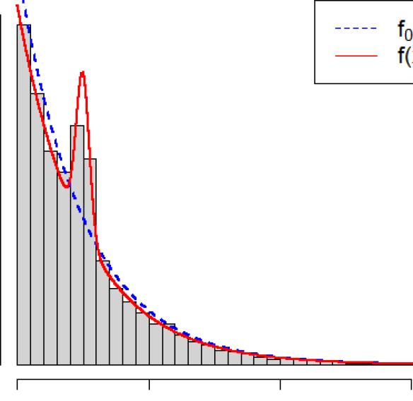
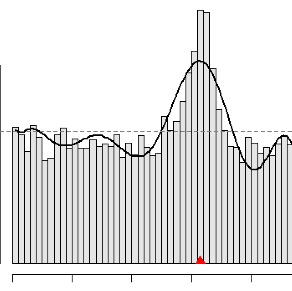
Figure 1: How closely does reality resemble the model? $10,000$ samples are generated from the true (unknown to the analyst) model $0.9{\rm Exp}(\lambda_{0})+0.1\mathcal{N}(25,2.5^{2})$. The right plot shows the graph of $\widehat{d}_{0}(x)$, which acts as a ‘magnifying glass’ that forces us to examine what extra information data are willing to reveal beyond the known assumed model. The crucial point here is: model uncertainty, as captured by $\widehat{d}_{0}(x)$, has a shape—it is not a single numeric number. It helps physicists narrow down a large set of potential rival theories to a few plausible ones.

2.3.1 Graphical Exploration of Model Uncertainty

Example 1.

Consider the following scenario: Fig. 1 displays the data that a physicist just collected from an experiment. The blue curve is the physics-informed background distribution $f_{0}(x)$, which, in this case, is an exponential distribution with $\lambda_{0}=25$, and the red curve is the true unknown probability distribution. The physicist is mainly interested in knowing whether there is any new physics hidden in the data, i.e., anything new in the data that was overlooked by existing theory. If so, what is it? How does the theory ($f_{0}$) relate to practice? This will help the physicist to come up with some scientific explanations and potential alternative theories.

The Shape of Uncertainty. The researcher ran the density-sharpening algorithm of the previous section with $m=10$, and the resulting $\widehat{d}_{0}(x)$ is displayed in the right of Fig. 1 as a function of $F_{0}(x)$. Few conclusions: (i) Model appraisal: The non-uniformity of $\widehat{d}$ tells us that the “shape of the data” is inconsistent with the presumed model-0. (ii) Model amendment: The shape of $\widehat{d}$ also informs the scientist about the nature of deficiency of the old model—i.e., what are the most worrisome aspects of the presumed model? In this example, the most consequential unanticipated pattern is the presence of a prominent ‘bump’ (excess mass) around $F_{0}^{-1}(0.63)\approx 24.85$, which might be indicative of new physics. This newly discovered pattern can now be used to improve the background exponential model.

Remark 2 (Visual explanatory decision-aiding tool).

One of the unique abilities of our exploratory learning is its ability to generate explanations on why and how the model-0 is incomplete. Thus, the graph of $\widehat{d}(u;F_{0},F)$ explicitly addresses decision-makers model misspecification concerns. It digs into the observations to uncover the “blind spots” of the current model that can ultimately drive discovery (locating novel hypotheses) and better decisions.

2.3.2 Measure of Model Uncertainty

A general measure of the degree of model misspecification is defined using the Csiszár information divergence class.

Definition 3.

For $\psi:[0,\infty)\mapsto\mathbb{R}$ a convex function with $\psi(1)=0$, define the Csiszár class of statistical divergence measure between $F$ and $F_{0}$:

$$I_{\psi}(F,F_{0})\,=\,\int_{-\infty}^{\infty}\psi\left(\frac{f(x)}{f_{0}(x)}\right)f_{0}(x)\;\mathrm{d}x$$ (15)

We prefer to represent it in terms of density-sharpening function as follows:

$$I_{\psi}(F,F_{0}) = \int_{-\infty}^{\infty}\psi\circ d(F_{0}(x);F_{0},F)\;\mathrm{d}F_{0}(x)\leavevmode\nobreak\ \leavevmode\nobreak\ \leavevmode\nobreak\ \leavevmode\nobreak\$$ (16)

$$= \int_{0}^{1}\psi\circ d(u;F_{0},F)\;\mathrm{d}u,\leavevmode\nobreak\ \leavevmode\nobreak\ \text{where}\leavevmode\nobreak\ u=F_{0}(x).\leavevmode\nobreak\ \leavevmode\nobreak\ \leavevmode\nobreak\ \leavevmode\nobreak\$$

One can recover popular divergence measures by appropriately choosing the $\psi$-function:

• KL-divergence: $\psi(x)=x\log(x)$; $I_{{\rm KL}}(F,F_{0})=\int d\log d$.

• Total variation divergence: $\psi(x)=|x-1|$; $I_{{\rm TV}}(F,F_{0})=\int|d-1|$.

• Squared Hellinger distance: $\psi(x)=(1-\sqrt{x})^{2}$; $I_{{\rm H}}(F,F_{0})=\int(1-\sqrt{d})^{2}$.

• $\chi^{2}$-divergence: $\psi(x)=(x-1)^{2}$; $I_{\chi^{2}}(F,F_{0})=\int(d-1)^{2}=\int d^{2}-1$.

One can quickly estimate the $\chi^{2}$-model misspecification index by expressing it in terms of LP-Fourier coefficients (applying Parseval’s identity to equation 9):

$$I_{\chi^{2}}(F,F_{0})=\int d^{2}-1=\sum_{j=1}^{m}\big{|}\operatorname{LP}[j;F_{0},F]\big{|}^{2}.$$ (17)

$I_{\chi^{2}}(F,F_{0})$ quantifies the uncertainty of the preliminary model $f_{0}(x)$ in light of the given data—i.e., whether $f_{0}(x)$ is catastrophically wrong or slightly wrong. Estimate it by plugging the empirical LP-coefficients (12) into (17). Since, under $H_{0}:F=F_{0}$, the sample LP-coefficients have the following limiting null distribution (see Theorem 2 of Mukhopadhyay 2017):

$$\sqrt{n}\widetilde{\operatorname{LP}}[j,F_{0},F]\xrightarrow[]{d}\mathcal{N}(0,1),\leavevmode\nobreak\ \leavevmode\nobreak\ \textrm{i.i.d for all}\leavevmode\nobreak\ j,$$

$n\widetilde{I}_{\chi^{2}}(F,F_{0})$ follows $\chi^{2}_{m}$ under null. One can use this to compute the $p$-value. Applying this measure to example 1, we get a $p$-value of practically zero—indicating that the background exponential model is badly damaged and should be repaired before making a decision.

Remark 3.

It is interesting to contrast our theory with Hansen and Sargent (2022, Sec. 4 and 5.1), keeping in mind that their $m(x)$ is exactly our sharpening function $d_{0}(x)$. This reinforces our belief that our theory can be applied broadly to econometrics and decision-making under uncertainty.

2.4 $d$-Sharp Models

Definition 4.

$\operatorname{DS}(F_{0},m)$ stands for Density-Sharpening of $f_{0}(x)$ using $m$-term LP-series approximated $d_{0}(x)$, given by:

$$\leavevmode\nobreak\ \leavevmode\nobreak\ \leavevmode\nobreak\ f(x)\,=\,f_{0}(x)\Big{[}1\,+\,\sum_{j=1}^{m}\operatorname{LP}[j;F_{0},F]\,T_{j}(x;F_{0})\Big{]},\leavevmode\nobreak\ \leavevmode\nobreak\ \leavevmode\nobreak\ \leavevmode\nobreak\ \leavevmode\nobreak\$$ (18)

obtained by replacing (9) into (2). $\operatorname{DS}(F_{0},m)$ generates a relevant class of plausible models in the neighbourhood of the postulated $f_{0}(x)$ that are worthy of consideration.

A few additional points on density-sharpening:

1. The $\operatorname{DS}(F_{0},m)$-based density-sharpening principle provides a mechanism for exploring data by exploiting the uncertain background knowledge model. It starts with data and an approximate model $f_{0}(x)$—and produces a more refined picture of reality following (18).

2. The process of density-sharpening suitably ‘stretches’ the theory-informed model to create a class of robust empirico-scientific models. Moreover, it shows how new models are born out of data-driven mutation of pre-existing ones.

3. The truncation point $m$ indicates the radius of the neighborhood around the elicited $f_{0}(x)$ to create permissible models. $\operatorname{DS}(F_{0},m)$ models with higher $m$ entertain alternative models of higher complexity. However, to maintain conceptual appeal and interpretability, it is advisable to focus on the vicinity of $f_{0}$ by choosing an $m$ that is not too large. Substituting the smooth estimates $\widehat{\operatorname{LP}}[j;F_{0},F]$ of eq. (14) into the formula (18), we get the most economical model (among competing alternatives around $f_{0}$) that best explains the empirical surprise.

4. It provides an architecture of an ‘intelligent agent’ that simultaneously possesses the ability to: learn (what’s new can we learn from the data), reason (how to explain the surprising empirical findings), and plan (how to self-modify to adapt in the new situations).

Example 2 (Glomerular filtration data).

We are given glomerular filtration rates for 211 kidney patients. The experiment was done at Dr. Bryan Myers’ Nephrology research lab at Stanford University. The dataset was previously analyzed in Efron and Hastie (2016).

The blue curve on the left plot of Fig. 2 shows the best-fitted lognormal (LN) distribution. We start our analysis by asking whether the parametric LN model needs to be refined to fit the data. The middle panel displays the density-sharpening function, which provides insights into the nature of misspecification of the LN model: the peak and the tails of the initial LN distribution need repairing; LN underestimates the peak and neglects the presence of heavier tails. The repaired LN model (displayed on right-hand side of Fig. 2) is given by

$$\widehat{f}(x)\,=\,f_{0}(x)\big{[}1\,+\,0.18T_{4}(x;F_{0})\big{]},$$ (19)

where $f_{0}(x)$ is ${\rm LN}(\mu_{0},\sigma_{0})$, with $\mu_{0}=4$ and $\sigma_{0}=0.24$. The part in the square bracket comes from $d_{0}(x)$, which provides recommendations on how to suitably elaborate the LN-model to capture the unexplained shape. The point of this example was to show how the density-sharpening principle (DSP) allows an analyst to explicitly perform model formulation, fitting, checking, and repairing—all seamlessly combined into one workflow.

It is interesting to compare our $d$-sharp LN-model (the red curve) with the seven-parameter exponential family fit shown in Fig. 5.7 of Efron and Hastie (2016). The most noticeable difference lies in the right tail. Efron’s seven-parameter exponential family model shows weird spikes on the extreme-right tail. The main reason for this is that it is based on polynomials of raw $x$: ($x,x^{2},\ldots,x^{7}$), which are not robust. That is to say, these traditional bases are unbounded and highly sensitive to ‘large’ data points. In contrast, our LP-polynomials are functions of $F_{0}(x)$, not raw $x$, and thus robust by design. The other operational difference between our approach and Efron’s exponential family approach is that we model the “gap” between lognormal and the data, which is often far easier to approximate nonparametrically (only required one parameter, see eq. 19) than modeling the data from scratch.

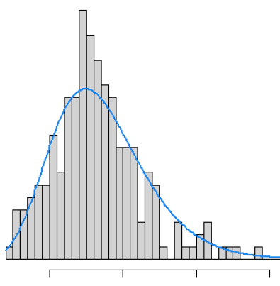
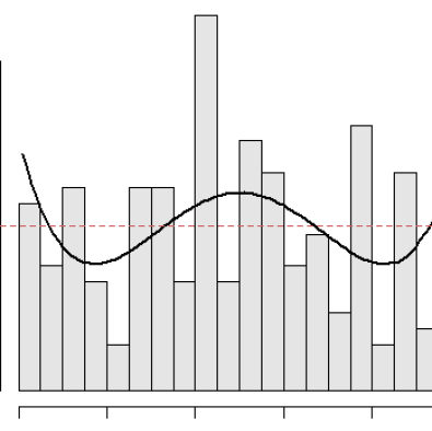
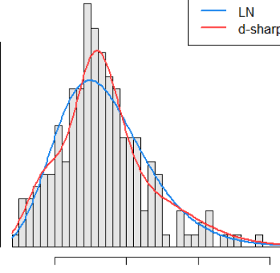
Figure 2: Glomerular filtration data modeling. Left: the fitted lognormal distribution. Middle: The estimated density-sharpening function $d_{0}$ provides an economical description of the empirical surprise, thereby supplying clues for forming new explanatory hypotheses of the data. Right: the $d$-sharp lognormal with heavier tails and sharper peak.

2.5 Modelplasticity and Abductive Inference Machine

Not the smallest advance can be made in knowledge beyond the stage of vacant staring, without making an abduction at every step. — C. S. Peirce (1901)

Modelplasticity—Models ability to modify and adapt itself in response to new data. The density-sharpening principle enables the model to develop new shapes in the face of change.

Density-sharpening and model evolution. Modeling is a continual process, not a one-time data-fitting exercise. The density sharpening mechanism allows us to combine new observations with a priory expected model to generate new insights, as depicted in Fig. 3.

Figure 3: Architecture of abductive inference machine (AIM). Density-sharpening principle provides a systematic process of inserting the new information into the existing knowledge model to resolve empirical surprise and inconsistency. This continuous cycle of iterative model sharpening is called abductive learning, which facilitates the emergence of new theories from data. As George Box (1980) said, ‘The statistician’s role is to assist this evolution.’

Statistical law of model evolution. Density-sharpening supports this dynamic process of recursive model upgrading: $f_{k}(x)=f_{k-1}(x)\,d_{k-1}(x)$, for $k=1,2,\ldots$, by allowing the model to constantly evolve and reshape itself with fresh sets of data—going from a simple approximate model to a much more mature, accurate model of reality.

Abduction and creation of new knowledge. Abduction is the creative part of an inferential process that aims at producing new theories from data. It builds upon what we know to discover new facts about nature. Abductive learning is concerned with the following questions: What new can we learn from the data? How to change the prior hypothetical model to explain the current situation? Which alternative classes of models are worthy of being entertained?

‘Does statistics help in the search for an alternative hypothesis? There is no codified statistical methodology for this purpose. Text books on statistics do not discuss either in general terms or through examples how to elicit clues from data to formulate an alternative hypothesis or theory when a given hypothesis is rejected.’

— C. R. Rao (2001)

Charles Sanders Peirce (1837–1914) was the pioneer of abductive reasoning; see Stigler (1978) and Mukhopadhyay (2023) for more details on the Peircean view of statistical modeling. The goal of Abductive Inference Machine or AIM is to provide a learning framework that endows a model with this ability to learn, grow and change with new information.

Remark 4.

The density-sharpening process plays an essential role for abductive inference, which provides the computational machinery for generating novel hypotheses with explanatory merit and selecting specific ones for further examinations.

Remark 5 (Abductive inference $\neq$ Hypothesis testing).

Any scientific inquiry begins with observations and some initial hypotheses. Classical statistical inference develops tools to test the validity of the null model in light of the data. Since all scientific theories are incomplete, accepting or rejecting a particular hypothesis is a pointless exercise. The real question is not whether the null hypothesis is true or false. The real question is: how far is the reality from the postulated model? In which direction(s) should we search to find a better model? Density-sharpening law provides a process of progressive refinement of yesterday’s hypothesis.

2.6 Attention Mechanism

We often neglect how we get rid of the things that are less important…And oftentimes, I think that’s a more efficient way of dealing with information.

— Duje Tadin

Attention is the prerequisite of gaining new knowledge. Intelligent learners have the ability to quickly infer where to focus attention to gain knowledge. In our modeling framework $d_{0}(x)$ draws analyst’s attention quickly and efficiently to the new informative part by suppressing boring details; verify it from the graphs of $d_{0}(x)$ in Figs. 1 and 2. It acts as a ‘gating mechanism’ that filters out the new interesting (surprising) aspects of the data, and ignores the dull and unsurprising part—thereby sharpening the model’s intelligence by guiding where to pay attention for information processing.

“The whole function of the brain is summed up in: error-correction”                   — W. Ross Ashby, English psychiatrist and a pioneer in cybernetics.

Remark 6.

In the brain, a dedicated circuit (or system) performs information-filtering similar to what $d_{0}(x)$ does for our dyadic model. The existence of such a brain circuit was first hypothesized by Francis Crick (1984)—he called it ‘The Searchlight Hypothesis.’ Since then, significant progress has been made to hunt down the brain region, what is now called basal ganglia, that suppresses irrelevant inputs. For more details see Halassa and Kastner (2017) and Gu et al. (2021). Basal ganglia help us focus on what’s important and tune out the rest. The mechanics of our model-building mimic the brain’s cognitive process that uses existing knowledge to sieve out the new information for correcting the error (sharpening) of the earlier mental model.

3 Decision-Making with Imperfect Model

How should a decision maker acknowledge model misspecification in a way that guides the use of purposefully simplified models sensibly?

— Cerreia-Vioglio et al. (2020)

This section demonstrates how practicing abductive inference based on the density-sharpening principle can enable better decision-making in highly uncertain environments.

3.1 Abductive Model of Decision Making

Abduction is the process of generating and revising a model before choosing the optimal action. An abducer makes decisions in a dynamic uncertain environment by allowing for potential model misspecification. Abductive decision-making is about knowing when to change course and how to change it.

How can a decision-maker abduct? The mechanics of abductive decision-making consist of three steps: (i) generating a set of plausible alternative models based on new evidence; (ii) constructing a ‘robust’ model (by choosing the least favorable alternative model or by averaging the alternative models with proper weights); and (iii) selecting an action that maximizes expected utility under the newly revised model. Two modes of abductive decision-making under uncertainty are presented below.

Notation. A decision-maker (DM) has to take an action $a$ from the set of available actions $\mathbb{A}=\{a_{1},\ldots,a_{q}\}$ based on observed outcome $X_{1},\ldots,X_{n}$ from an unknown probability distribution $f(x)$, representing some natural or social phenomenon. The DM selects the optimal action that minimizes expected loss (or risk) under the assumed model-0:

$$\widehat{a}_{0}:=\operatorname{argmin}_{a\in\mathbb{A}}\int L_{a}(x)\;\mathrm{d}F_{0}(x),$$ (20)

where $f_{0}(x)$ is the DM’s posited probability distribution over outcomes. However, as an abducer, the DM is completely aware that the uncertainty about the outcomes may not be fully captured by a single, rigidly-defined probability distribution $f_{0}(x)$ and thus wants to choose the best decision by accommodating the uncertainty of model-0.

Decision making based on density sharpening principle. To account for the imperfect nature of model-0, the most natural thing to do is to work with an enlarged class of plausible distributions around the vaguely acceptable $f_{0}(x)$:

$$\Gamma_{M}\leavevmode\nobreak\ =\leavevmode\nobreak\ \big{\{}f:\,f\in\operatorname{DS}(F_{0},m),\leavevmode\nobreak\ m\leq M\big{\}}$$ (21)

within a certain reasonable neighbourhood, say $M=10$. We like to use this enlarged class of distributions $\Gamma_{M}$ for robust decision-making. Two such strategies are discussed below.

Method 1. A cautious DM selects an action by its expected loss under the least favourable distribution within the set $\Gamma_{M}$:

$$\breve{f}_{a,M}\,=\,\operatorname*{arg\,sup}_{F\in\Gamma_{M}}\int L_{a}(x)\;\mathrm{d}F(x).$$ (22)

We call this an abductive-minimax procedure. Our proposal is partly inspired by the ‘local-minimax’ idea of Hansen and Sargent (2001a, b).

Method 2. We now describe another robust decision-making procedure that takes into account the uncertainty in the analyst’s elicited probability model of future states. Two key concepts are: bootstrap model averaging and action-profile function.  Step 1. We use bootstrap to explore $f\in\Gamma_{M}$ in an intelligent way. Draw $n$ samples with replacement from the original data. Denote the bootstrap empirical cdf as $\widetilde{F}_{*}^{(1)}$. Perform density-sharpening algorithm based on $\widetilde{F}_{*}^{(1)}$, and denote the estimated $d$-sharp model as $f_{*}^{(1)}$.

Step 2. Use $f_{*}^{(1)}$ to select the best action from the given set of $q$-actions $\{a_{1},\ldots,a_{q}\}$. Denote the selected action as $a_{*}^{(1)}$.

Step 3. Repeat steps 1-2, $B$ times (say $B=1000$ times). And return:

• The sample bootstrap distribution $p_{A}$ of optimal actions $\{a_{*}^{(1)},\ldots,a_{*}^{(B)}\}$—which we call the action profile of the decision problem.

• Bootstrap systematically generates probable alternative models $\{f_{*}^{(1)}(x),\ldots,f_{*}^{(B)}(x)\}$ from the class $\Gamma_{M}$ that can explain the data. Compute bootstrap model averaged distribution:

  $$\bar{f}(x)\,=\,\frac{1}{B}\sum_{j=1}^{B}f_{*}^{(j)}(x).\leavevmode\nobreak\ \leavevmode\nobreak\ \leavevmode\nobreak\ \leavevmode\nobreak\ \leavevmode\nobreak\$$ (23)

  By averaging all plausible alternatives, $\bar{f}(x)$ becomes robust to model uncertainty. In this strategy, the policymaker does not have to put his/her complete faith in a single alternative distribution to assign probabilities. Bootstrap density exploration generates and weights different alternatives (from the class $\Gamma_{m}$) appropriately to create a realistic model. Fig. 4 shows the bootstrap-generated densities for the gfr data of example 2. The light blue curves are the plausible alternative models, and the dark blue is the averaged density that takes into account all likely scenarios. It’s worth contrasting $\bar{f}(x)$ with more traditional parametric uncertainty-based Bayesian predictive density; see supplementary A1.

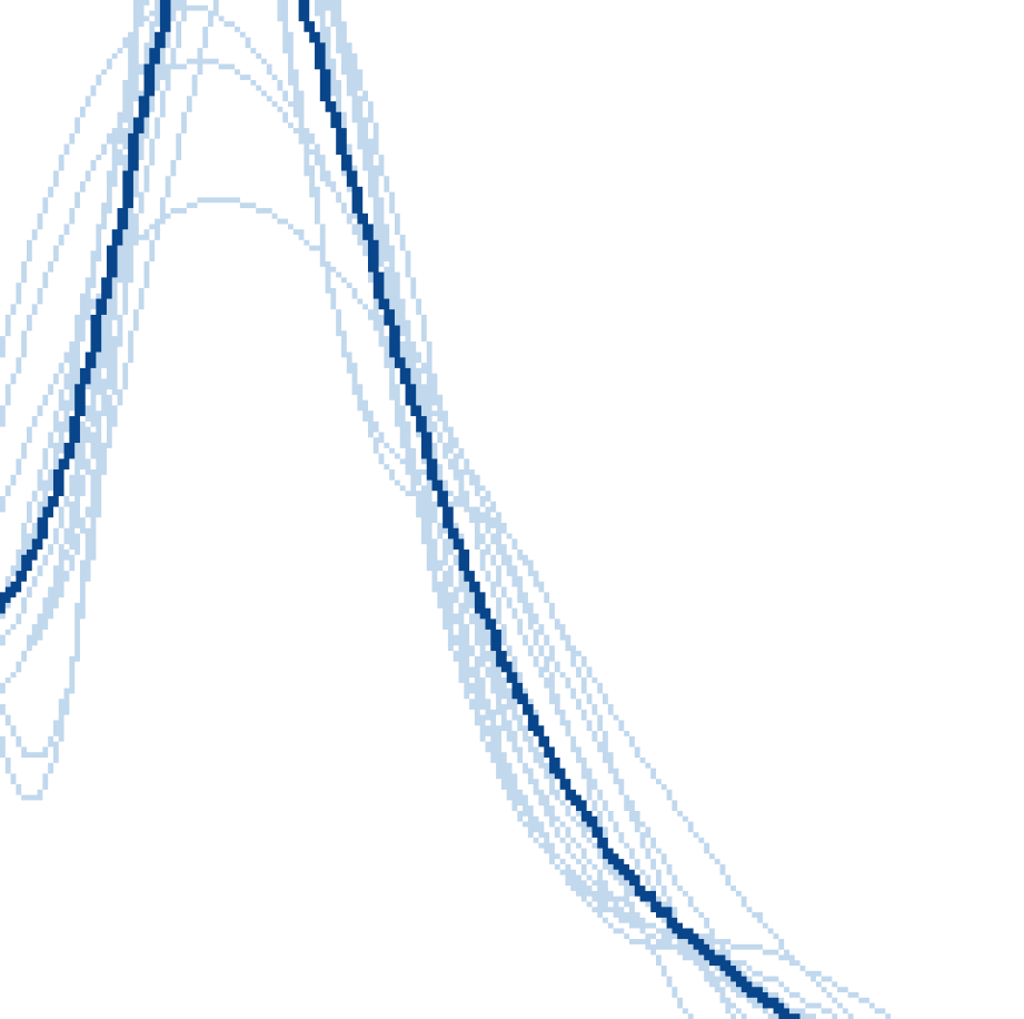
Figure 4: The light blue curves are the bootstrap generated gfr densities, which try to present a landscape of plausible scenarios as suggested by the data. The dark blue denote the estimated model-averaged distribution $\bar{f}(x)$, which takes into account the uncertainty surrounding the initially postulated model $f_{0}(x)$ as captured by the class $\Gamma_{M}$.

Remark 7.

Two remarks: (i) Rather than assuming that alternative probable models are given to us a priori, we use density-sharpening-based abductive inference method to synthesize them, allowing us to account for a much broader range of model uncertainty than is possible with conventional approaches like Bayesian model averaging; see Supp. note A4. (ii) Furthermore, in our scheme, bootstrap provides a way to automatically estimate the posterior probability of accepting each synthesized alternative model (light blue curves in Fig. 4), eliminating the need for arbitrary subjective probabilities over models. To compute the $\bar{f}$, bootstrap-derived model posterior probabilities are used to weigh the various alternatives from the density-set $\Gamma_{M}$; see Supp. note A3.

Step 4. This bootstrap scheme can also be used to approximately compute the least favourable distribution, defined in (22):

$$\breve{\breve{f}}_{a,M}=\operatorname{argmax}_{j}\int L_{a}(x)\;\mathrm{d}F_{*}^{(j)}(x).$$

The decision-maker can use this estimated model to carry out the proposed abductive-minimax procedure (method 1).

Step 5. Robust procedure: A pragmatic decision-maker chooses an action (or ranks the actions) that minimizes expected loss (or maximizes the expected utility) with respect to the averaged-distribution: $\widehat{a}_{{\rm robust}}:=\operatorname{argmin}_{a\in\mathbb{A}}\int L_{a}(x)\;\mathrm{d}\bar{F}(x)$. Our strategy prescribes action that is robust across a wide range of plausible alternative models. It could be especially powerful for dealing with “deep uncertainty” in making robust policies. For a comprehensive overview on this subject, see Marchau et al. (2019).

Step 6. Quantifying the ‘robustness’ of the action (or decision rule): How much does the optimal action change when a model is selected from a reasonable neighborhood of the assumed initial opinion, i.e. from the $\Gamma_{m}$ class? The shape of the action profile distribution can be used to determine how robust the optimal action is to model perturbation. In particular, the entropy of the action profile distribution can be used to assess the robustness (or stability) of the inference to potential model misspecification:

$${\rm Entropy}[p_{A}]\,=\,-\sum_{i=1}^{q}p_{A}(i)\,\log p_{A}(i)=\,-\sum_{i=1}^{q}\Pr(A=a_{i})\,\log\Pr(A=a_{i}).$$ (24)

Uniform probability over possible actions yields maximum uncertainty—indicating that the decision is highly non-robust (sensitive) to model misspecification.

3.2 Quantile Decision Analysis

Until now, we have assumed experts can precisely formulate their opinion in a probabilistic form $f_{0}(x)$. However, for complex real-world decision-making problems, experts might only have incomplete information about the uncertainty distribution of the target variable. A decision-analyst often elicit their partial knowledge about an uncertain quantity as a set of quantile-probability (QP) pairs $\{x_{i},F(x_{i})\}$, for $i=1,\ldots,\ell$. The job of an analyst is to find a simple, flexible, and parameterizable density that honors the assessed percentiles.

Model ambiguity due to incomplete information. The task of eliciting an expert’s probability distribution from a small set of QP pairs is a vital yet nascent topic in decision analysis; see Powley (2013), Keelin and Powley (2011), Hadlock (2017). In this section, we present an algorithm called Q2D (stands for quantile to distribution) that provides a systematic approach to deduce a reliable expert distribution from $\ell$ arbitrary QP-specifications.

Probability-gap Approximation. The main theoretical idea behind Q2D algorithm: Recall our $\operatorname{DS}(F_{0},m)$ model

$$f(x)\,=\,f_{0}(x)\Big{[}1\,+\,\sum_{j=1}^{m}\operatorname{LP}[j;F_{0},F]\,T_{j}(x;F_{0})\Big{]}\leavevmode\nobreak\ \leavevmode\nobreak\ \leavevmode\nobreak\$$ (25)

Integrating from minus infinity to $x$ on both sides, we have

$$\int_{-\infty}^{x}(f(z)-f_{0}(z))\;\mathrm{d}z=\sum_{j=1}^{m}\operatorname{LP}[j;F_{0},F]\int_{-\infty}^{x}S_{j}(F_{0}(z))\;\mathrm{d}F_{0}(z),$$

where $S_{j}(u)=T_{j}(Q_{0}(u);F_{0})$ is defined over the unit interval $[0,1]$ and $Q_{0}(u)$ is the quantile function of the distribution $f_{0}$. This leads to

$$F(x)-F_{0}(x)\,=\,\sum_{j=1}^{m}\operatorname{LP}[j;F_{0},F]\int_{0}^{F_{0}(x)}S_{j}(u)\;\mathrm{d}u.$$ (26)

Given a set of arbitrary $\ell$ quantile-probability data $(x_{i},F(x_{i})),$ for $i=1,\ldots,\ell$, we can rewrite (26) compactly as a matrix equation

$$v=S_{0}\bm{\beta}$$ (27)

where $v_{i}=F(x_{i})-F_{0}(x_{i})$, $\beta_{i}=\operatorname{LP}_{j}$, and $S_{0}\in\mathcal{R}^{\ell\times m}$, $S_{0}[i,j]=\int_{0}^{F_{0}(x_{i})}S_{j}(u)$. The desired parameters are ${\bm{\beta}}=(\beta_{1},\ldots,\beta_{m})$, where $\beta_{j}$ is shorthand for $\operatorname{LP}[j;F_{0},F]$.

For $m\leq\ell$, we can uniquely estimate $\bm{\beta}$ using the least-square method

$$\widetilde{\bm{\beta}}\,=\,\operatorname*{minimize}_{\bm{\beta}}\|v-S_{0}\bm{\beta}\|^{2}\,=\,(S_{0}^{T}S_{0})^{-1}S_{0}^{T}v.$$ (28)

For large $\ell$ (say, $\ell\geq 5$), a better, more stable estimate can be found through regularization

$$\widehat{\bm{\beta}}\,=\,\operatorname*{minimize}_{\bm{\beta}}\|v-S_{0}\bm{\beta}\|^{2}\leavevmode\nobreak\ +\leavevmode\nobreak\ \lambda\|\bm{\beta}\|_{1}$$ (29)

where $\|\cdot\|_{p}$ is the $\ell_{p}$ norm, and $\lambda>0$ is the regularization parameter. The lasso (Tibshirani, 1996) penalized $\widehat{\bm{\beta}}$ yields a sparse estimate and counters over-fitting. This penalized estimate provides a tradeoff between accuracy and interpretability. Finally, plug the estimated LP-Fourier coefficients $\beta_{j}$ into the primary equation (18) to get the expert distribution.

Remark 8.

The expert quantile specifications should not be viewed as a ‘gold standard’—they are nothing but a preliminary guess (prone to errors of judgment or hindsight bias) whose purpose is to steer the analyst in the right direction. For that reason, we recommend the smoothed (denoised) regularized $\widehat{\bm{\beta}}$ over the naive $\widetilde{\bm{\beta}}$, since it makes little sense to find an exact fit to the noisy QP-data.

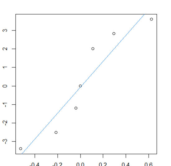
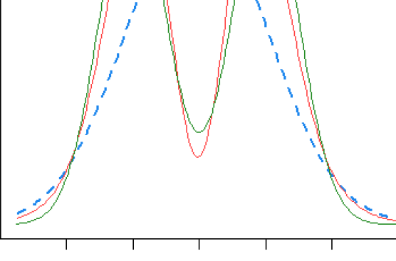
Figure 5: Learning from incomplete information. Left panel: Regression on the scatter $(\Phi^{-1}(u_{i}),Q(u_{i}))$, $i=1,\ldots,7$. Right panel: The blue dotted line is the estimated $f_{0}$: normal distribution. Q2D estimated curve is shown in red, which is impressively close to the true mixture density $\frac{1}{2}\mathcal{N}(-2,1)+\frac{1}{2}\mathcal{N}(2,1)$.

Example 3 (Bimodal Distribution).

We are given the following quantile judgments:

Quantile: $x_{i}$	-3.40	-2.53	-1.20	0	2.0	2.83	3.60
Probability: $F(x_{i})$	0.04	0.15	0.39	0.50	0.75	0.90	0.97

In our Q2D algorithm, we choose $F_{0}$ (an initial approximate shape) to be normal distribution. To estimate the parameters $\mu_{0}$ and $\sigma_{0}$ of the normal distribution, note that the quantile function $Q(u)\approx\mu_{0}+\sigma_{0}\Phi^{-1}(u)$. Thus one can quickly get a rough estimate by simply performing a linear regression on $(\Phi^{-1}(u_{i}),Q(u_{i}))$; see Fig. 5. The estimated normal distribution is shown in the right panel, along with the Q2D-estimated density.

Example 4 (U.S. Navy data).

Fig. 6 shows a histogram of 122 repair times (in hours) for a component of a U.S. Navy weapons system. The dataset was analyzed in Law (2011). Imagine that for privacy and other reasons, we do not have access to the full data. The goal is to infer a probability distribution that faithfully represents the following quantiles:

Quantile: $x_{i}$	0.12	1.30	3.00	7.00	26.17
Probability: $F(x_{i})$	0.01	0.20	0.50	0.80	0.99

We start with exponential distribution as our initial guess, which is often taken as a ‘default’ distribution (model-0) in reliability analysis. For $X\sim{\rm Exp}(\lambda)$, we have

$${\rm Median}(X)\,=\,\lambda\ln(2),\leavevmode\nobreak\ \leavevmode\nobreak\ {\rm where}\leavevmode\nobreak\ \lambda=\mathbb{E}(X).\leavevmode\nobreak\ \leavevmode\nobreak\$$

From the quantile table we get $\hat{\lambda}=3/\ln(2)=4.32.$ Next, we apply the Q2D algorithm to derive the LP-parameters with $f_{0}={\rm Exp}(4.32)$. The resulting density sharpening function and the final $d$-sharp exponential are shown in Fig. 6. The red curve on the right plot shows an excellent fit to the data, which was derived by the Q2D algorithm simply by utilizing the five quantile-probability pairs.

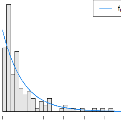
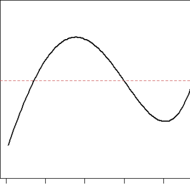
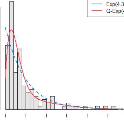
Figure 6: Left: histogram of 122 repair times for a component of a U.S. Navy weapons system. The blue curve is the $f_{0}={\rm Exp}(4.32)$. Our analysis only used five QP-data (not the full data), whose outputs are shown in the middle and right-hand panels. The inferred density-sharpening function tells that the peak and the tail of the exponential model need correction. The repaired exponential model is displayed in red.

3.3 Decision-making based on Multiple Experts

High-stakes decision-making (say, COVID-19 pandemic or climate change) is often based on multiple experts’ opinions instead of putting all bets on a single rigidly-defined probability model. The challenge is to aid data-driven decision-making by appropriately combining several experts’ models. We describe one possible way to build a ‘consensus committee model’ that can be used as a possible model-0 within an abductive decision-making framework.

Learning from multiple expert distributions. Given $k$ competing probability models $\{f_{01},\ldots,f_{0k}\}$, which may differ markedly in shape, define the following model-weights:

$$\text{Relevance weight:}\leavevmode\nobreak\ \leavevmode\nobreak\ \leavevmode\nobreak\ \leavevmode\nobreak\ \leavevmode\nobreak\ \leavevmode\nobreak\ w_{\ell}=\dfrac{1}{1+\sum_{j}|\operatorname{LP}_{j|\ell}|^{2}},\leavevmode\nobreak\ \leavevmode\nobreak\ \leavevmode\nobreak\ \leavevmode\nobreak\ {\rm for}\leavevmode\nobreak\ \ell=1,\ldots,k\leavevmode\nobreak\ \leavevmode\nobreak\ \leavevmode\nobreak\ \leavevmode\nobreak\ \leavevmode\nobreak\ \leavevmode\nobreak\ \leavevmode\nobreak\ \leavevmode\nobreak\ \leavevmode\nobreak\ \leavevmode\nobreak\$$ (30)

where $\operatorname{LP}_{j|\ell}$ is the LP-Fourier coefficients of the $\ell$-th model:

$$d_{0\ell}(x):=d(F_{0\ell}(x);F_{0\ell},\widetilde{F})\,=\,1+\sum_{j}\operatorname{LP}_{j|\ell}T_{j}(x;F_{0\ell}).$$ (31)

Note that the relevance weight for the $\ell$-th model is always $0<w_{\ell}\leq 1$, and

$$w_{\ell}=1\leavevmode\nobreak\ \leavevmode\nobreak\ \leavevmode\nobreak\ \text{if and only if}\leavevmode\nobreak\ \leavevmode\nobreak\ \leavevmode\nobreak\ \operatorname{LP}_{j|\ell}=0,\leavevmode\nobreak\ \forall\leavevmode\nobreak\ j.\leavevmode\nobreak\ \leavevmode\nobreak\$$

$\operatorname{LP}_{j|\ell}=0$ for all $j$ when $f_{0\ell}$ fully explain the data and there is no need to sharpen it further (i.e., $d_{0\ell}=1$). In that sense, $w_{\ell}$’s are data-driven weights (which will keep changing as we get more and more fresh data), computed based on the degree of agreement between the observed data and expert model $f_{0\ell}$. Define mixture expert distribution as

$$f^{0}_{\rm mix}(x)\leavevmode\nobreak\ =\leavevmode\nobreak\ \sum_{\ell=1}^{k}\pi_{\ell}\,f_{0\ell}(x),\leavevmode\nobreak\ \leavevmode\nobreak\ \leavevmode\nobreak\$$ (32)

where $\pi_{\ell}=w_{\ell}/\sum_{\ell}w_{\ell}$. This model serves two purposes: it tries to resolve conflicting opinions based on data and at the same time encourages one to include as much diverse information as possible.

Additional layer of model uncertainty. If the analyst believes that the correct model might not be among the collection of models being considered, then use the combined expert model $f^{0}_{\rm mix}(x)$ as a model-0 in the subsequent density-sharpening-based learning and abductive decision-making process.

4 Model Management Science

How should an analyst use imperfect models to learn from data? What should be the output of such an analysis that can ultimately aid informed decision-making? We address these questions by introducing a general inferential framework for statistical learning and decision-making under uncertainty—which builds on two core ideas: abductive thinking and density-sharpening principle. Some of the defining features of our approach for data analysis, scientific discovery, and decision-making are highlighted below:

$\bullet$ Data analysis and science of model management: No model is perfect, irrespective of how cunningly it is designed. The central problem of statistical model developmental process is to understand how a relatively simple model can evolve into a more complex and mature one in the presence of a new data environment. The principle of density-sharpening assists this model evolution process (thereby helping empirical scientists to abduct): by abductively generating explanations on why the presumed model-0 is unfit for the data [playing the role of a quality inspector] and also providing recommendations on how to fix the misspecification issues [serving as a policy adviser] in order to make better decisions in new circumstances.

$\bullet$ Discovery and creation of new knowledge: Abductive data analysts are less interested in testing a particular working model. They are mainly interested in conceptual innovation: discovering new pursuitworthy hypotheses based on surprising empirical evidence. The density-sharpening function $d(u;F_{0},F)$ picks out ‘what’s new’ in the data beyond the current scientific knowledge encoded in $f_{0}(x)$, thereby helping the scientist to uncover new unexpected knowledge from the data using graphical tools. The density-sharpening principle (DSP) provides a learning mechanism that isolates the ‘known’ from the ‘unknown’ and allows us to focus on the newfound pattern in the data, which is the basis for knowledge-creation.

$\bullet$ Abductive inference and decision-making: The proposed theory of abductive decision-making tackles model uncertainty induced by imprecise, ambiguous, and incomplete knowledge about the underlying probabilistic structure. An abductive-decision support system automatically discovers and explicitly articulates the possible alternatives to the analysts, which forces them to rethink their choices before taking impulsive action; see Supp. note A5. This style of empirical reasoning and adaptive decision-making could be especially valuable in situations where strategic planners need to take quick action in the face of uncertainty, equipped with approximate subject-matter knowledge.

Code and Data availability

All the datasets and R-code written for the analysis are available upon request to the author.

Ethical Statement

The Author declares that there is no conflict of interest/competing interests.

Supplementary material

For more discussion on how our abductive statistical approach compares to the more traditional Bayesian statistical approach for model misspecification, robustness, and decision-making, see the Supplementary section.

A Supplementary Notes

This supplementary section contains some additional notes on the connections and differences between the Bayesian statistical approach vs. the Abductive statistical approach to model misspecification, robustness, and decision-making.

A1. The two types of model-uncertainty: Parametric and nonparametric It is important to distinguish two main types of model uncertainty: parametric uncertainty and more general nonparametric shape uncertainty.

1) Parametric uncertainty is a classical scenario in which the model structure is assumed to be known but not the relevant parameter values. In this setup, it is implicitly assumed that the decision-maker is aware of the correct parameterized statistical models $f_{0}(\cdot;\theta)$, which is misspecified in terms of only $\theta$. We can therefore think of it as a finite-dimensional (statistical search) problem, for which we have a number of legacy theories, including Bayesian inference.

2) Under nonparametric shape uncertainty, we work with much deeper or more severe uncertainties about the shape of the data-generating model. It is a far more challenging infinite-dimensional (statistical search) problem for which there is no established general theory. This paper addresses this concern by offering a ‘general theory of nonparametric model revision’ whose foundation stands on two pillars: the density-sharpening principle and abductive inference. In our theoretical framework, we only have access to a probability model $f_{0}(x)$ that approximately encodes the decision-maker’s beliefs about the distribution of the observations. Our theory then provides a systematic method for searching a useful class of alternative models $\operatorname{DS}(F_{0},m)$ by ‘correcting’ (or sharpening) the hypothesized model $f_{0}$ in an automated data-driven manner.

A2. Bayesian statistical approach vs. Abductive statistical approach    1) Bayesian inference is extremely effective for dealing with parametric model uncertainty. Bayes’ law provides a principled method for updating beliefs about a model’s parameters.

Bayes’ law. Given observed data $x=(x_{1},\ldots,x_{n})$ and the parametrized likelihood function $f_{0}(x;\theta)$, Bayes’ multiplicative rule updates belief about $\theta$ from the prior to posterior as follows

$$\widetilde{\pi}(\theta|x)\leavevmode\nobreak\ \propto\leavevmode\nobreak\ \pi(\theta)\prod_{i=1}^{n}\{f_{0}(x_{i};\theta)\}.$$ (A.1)

For more details on standard methods for Bayesian parametric modeling, see Box (1980).

Bayes decision rule. Optimal Bayes action is taken by minimizing the expected loss under the posterior:

$$\hat{a}_{{\rm Bayes}}\leavevmode\nobreak\ :=\leavevmode\nobreak\ \operatorname{argmin}_{a\in\mathbb{A}}\int_{\Theta}L_{a}(\theta)\,\tilde{\pi}(\theta|x)\;\mathrm{d}\theta.$$

For more detailed treatment refer to the standard textbooks like Berger (2013, Chapter 4).

2) Abductive inference, on the other hand, is a powerful mode of statistical reasoning for nonparametric model uncertainty problems. In particular, the proposed density-sharpening law provides a systematic rule for updating the shape of a probability density model.

The abductive decision analysts do not live in a fantasy world where decision-makers pretend to know the ideal parametrized model for the data. A new class of abductive inference-based decision-theoretic models called “dyadic models” are introduced in this paper (see Sec. 2), which allow the analyst to automatically generate a class of probable alternative models from data without imposing any prior structural constraints.

A3. Bayes’ model synthesis process The goal of the “model synthesis problem” is to answer the following question:

Given a set of observations, how to systematically go about searching for a model superior to the one the decision-maker initially guessed?

Bayes model synthesis process (contrast this with the abductive model synthesis process given in Sec. 3.1, method 2) takes into account the uncertainty of $\theta$ as follows:

1. Simulate $\theta_{1},\ldots,\theta_{B}$ from the posterior distribution $\widetilde{\pi}(\theta|x)$, for some large $B$, say $1000$.

2. Generate a set of plausible parametric models for the data $\{f(x|\theta_{j})\}_{1\leq j\leq B}$.

3. Averaging over the posterior distribution: Compute the averaged density that accounts for the uncertainty of $\theta$ (compare this with density-sharpening based bootstrap averaging method, Eq. 23)

$$\bar{f}_{\theta}(x)=B^{-1}\sum_{j=1}^{B}f(x|\theta_{j}).$$ (A.2)

which is an approximation to the posterior predictive density

$$\bar{f}_{\theta}(x)\approx\int_{\Theta}f(x|\theta)\,\pi(\theta|x)\;\mathrm{d}\theta$$ (A.3)

The traditional frequentist point-estimate based $\hat{f}:=f(x;\hat{\theta})$ underestimates the uncertainty inherent in $\theta$, and as a result, it is much ‘narrower’ than the Bayes $\bar{f}_{\theta}(x)$. By averaging over the posterior distribution, $\bar{f}_{\theta}(x)$ restores the uncertainty lost when only a single $\hat{\theta}$ is used.

Remark 9.

Also see Remark 7, where bootstrap is used as the poor man’s Bayes posterior probability for each alternative model synthesized from the class $\operatorname{DS}(F_{0},m)$.

A4. Awareness of Unawareness In our abductive model synthesis process, as described in Sections 2 and 3.1, the crucial component is the dyadic model, which is founded on the density sharpening principle. One way to conceptualize dyadic models is as computational agents that are aware of their own unawareness. Using this model, decision-makers gain new previously unknown information that had been lurking in the shadows. As the analyst becomes aware of new facts, the belief is nonparametrically updated through the sharpening function $\widehat{d}_{0}(x)$. In other words, the sharpening function alerts decision-makers to their potential ignorance.

A5. Significance of abductive inference for decision making.    1) Adaptability. Reality always carries an element of surprise. To make effective decisions in a dynamic uncertain environment, it is critical to ensure that the decision model can withstand surprise; otherwise, it is unfit for use in the real world. The real advantage of using density-sharpening-based dyadic models is that they can recuperate from surprises through automated structural correction. As a result, an abductive decision rule based on dyadic models can adapt to surprises in the sense that if the true model deviates from the assumed one then still that decision works. This is achieved by averaging over the plausible alternative situations suggested by data, as described in section 3.

2) Explainability. Another advantage of abductive inference is that it provides an interpretable and transparent explanation of why and how the real world differs from decision-makers’ initial belief about the model, which is of utmost importance when advising on decisions to policymakers.

A6. Bayes, Smooth Bayes, Sharp Bayes, and Robust Bayes As an educated guess at the data-generation process, a decision analyst handpicks a class of parametric models $\{f_{0}(x;\theta):\theta\in\Theta\}$ with quantile function $Q_{0}(u;\theta)$ and cdf $F_{0}(x;\theta)$.

Definition 5 (Parametrized sharpening kernel).

Define the sharpening kernel between the true generating process $f(x)$ and the assumed parametrized $f_{0}(x;\theta)$ as

$$d_{\theta}\leavevmode\nobreak\ :=\leavevmode\nobreak\ d_{\theta}(u;F,F_{0}(\cdot;\theta))\leavevmode\nobreak\ =\leavevmode\nobreak\ \dfrac{f(Q_{0}(u;\theta))}{f_{0}(Q_{0}(u;\theta);\theta)},\leavevmode\nobreak\ \leavevmode\nobreak\ \,0<u<1\leavevmode\nobreak\ \leavevmode\nobreak\ \leavevmode\nobreak\ \leavevmode\nobreak\$$ (A.4)

The corresponding sample estimate is given by

$$\widetilde{d}_{\theta}\leavevmode\nobreak\ :=\leavevmode\nobreak\ d_{\theta}(u;\widetilde{F},F_{0}(\cdot;\theta))=\dfrac{\widetilde{f}(Q_{0}(u;\theta))}{f_{0}(Q_{0}(u;\theta);\theta)},\leavevmode\nobreak\ \leavevmode\nobreak\ \,0<u<1\leavevmode\nobreak\ \leavevmode\nobreak\ \leavevmode\nobreak\ \leavevmode\nobreak\$$ (A.5)

where $\widetilde{d}_{\theta}:\Theta\times[0,1]\rightarrow[0,\infty)$, which connects information in data to parameters of interest. With this definition in hand, we now present an important result.

Alternative representation of Bayes Rule. We express the likelihood-based standard Bayesian posterior update rule for $\theta$ as follows

$$\widetilde{\pi}(\theta|x)\leavevmode\nobreak\ \propto\leavevmode\nobreak\ \pi(\theta)\exp\big{\{}-\int\widetilde{d}_{\theta}\log\widetilde{d}_{\theta}\big{\}}.$$ (A.6)

This is equivalent to Eq. (A.1) becuase of the following fact

$$-\int\widetilde{d}_{\theta}\log\widetilde{d}_{\theta} = \int\log\{f_{0}(x_{i};\theta)\}\;\mathrm{d}\widetilde{F}\leavevmode\nobreak\ \leavevmode\nobreak\ +\leavevmode\nobreak\ \leavevmode\nobreak\ \text{constant}\leavevmode\nobreak\ \leavevmode\nobreak\$$ (A.7)

$$\propto \sum_{i=1}^{n}\log\{f_{0}(x_{i};\theta)\}.\leavevmode\nobreak\ \leavevmode\nobreak\$$ (A.8)

The Bayes rule is reformulated in terms of density sharpening kernel $\widetilde{d}_{\theta}$ because it offers a coherent and principled path for generalizing the belief update rule in situations where the probability model (likelihood function) is misspecified.

Smooth Bayes. Before delving into the Bayesian update rule under model misspecification, we describe “smooth” Bayes—an intriguing refinement of traditional Bayes. Substitute the noisy empirical $\widetilde{d}_{\theta}$ with the smoothed $\widehat{d}_{\theta}$ (following the method of Sec. 2.2) into Eq. (A.6) to get a smoothed version of the Bayes update rule:

$$\widehat{\pi}(\theta|x)\leavevmode\nobreak\ \propto\leavevmode\nobreak\ \pi(\theta)\exp\big{\{}-\int\widehat{d}_{\theta}\log\widehat{d}_{\theta}\big{\}},$$ (A.9)

Key assumption. Using the Savage axioms, the Bayesian update can be shown to be the rational way to make a decision when the guessed parametric family $\{f_{0}(x;\theta):\theta\in\Theta\}$ contains the true data model $f(x)$. However, this is a very stringent requirement that is difficult to meet in practice. We prefer to operate under more realistic conditions, which allows for $f_{0}(x;\theta)$ to be misspecified.

Sharp Bayes. What if the analysts’ a priori chosen family $\{f_{0}(\cdot;\theta):\theta\in\Theta\}$ does not contain the actual data generating model $f(x)$? It is well known that Bayes’ update exhibits undesirable characteristics under model misspecification.

Definition 6 (Generalized $d$-posteriors).

Define the following divergence-based generalized posterior density function

$$\pi(\theta|x)\leavevmode\nobreak\ \propto\leavevmode\nobreak\ \pi(\theta)\exp\big{\{}-I_{\psi}(F,F_{0}(\cdot;\theta))\,\big{\}}$$ (A.10)

where $I_{\psi}(F,F_{0}(\cdot;\theta))$ is the Csiszár class of divergence measure between the true data generator $f$ and the assumed misspecified class $f_{0}(\cdot;\theta)$. We refer to (A.10) as $d$-posterior, because we can rewrite it using Eq. (16) as

$$\pi(\theta|x)\leavevmode\nobreak\ \propto\leavevmode\nobreak\ \pi(\theta)\exp\big{\{}-\int\psi\circ d_{\theta}\big{\}}.\leavevmode\nobreak\ \leavevmode\nobreak\$$ (A.11)

whose sample estimate is given by

$$\widetilde{\pi}(\theta|x)\leavevmode\nobreak\ \propto\leavevmode\nobreak\ \pi(\theta)\exp\big{\{}-\int\psi\circ\widetilde{d}_{\theta}\big{\}}.\leavevmode\nobreak\ \leavevmode\nobreak\$$ (A.12)

In a remarkable result, Bissiri et al. (2016) showed that (A.12) provides a valid coherent rule for revising prior beliefs about the parameters of a model that is misspecified. Sharp-Bayes is the name given to this density-sharpening-based generalized Bayes update rule.

Remark 10 (The key idea).

The information in the observed data $x_{1},\ldots,x_{n}$ is connected with the parameter of interest $\theta$ via functionals of the sharpening function $\widetilde{d}_{\theta}$, instead of the conventional likelihood function, whose precise probability form is never known in practice.

Robust Bayes. For outlier-resistant robust Bayesian analysis choose total variation divergence, a special case of Csiszár class with $\psi(x)=|x-1|$ in (A.12)

$$\widetilde{\pi}(\theta|x)\leavevmode\nobreak\ \propto\leavevmode\nobreak\ \pi(\theta)\exp\big{\{}-\textstyle\int|\widetilde{d}_{\theta}-1|\big{\}}.$$ (A.13)

Another particularly useful class of measures for robust Bayesian analysis is Rényi $\alpha$-divergence, defined as

$$R_{\alpha}(F,F_{0})\,=\,\dfrac{1}{\alpha(1-\alpha)}\textstyle\Big{(}1-\int(f/f_{0})^{\alpha}\;\mathrm{d}F_{0}\Big{)},\leavevmode\nobreak\ \leavevmode\nobreak\ \leavevmode\nobreak\ \alpha\in\mathcal{R}\char 92\relax\{0,1\}.$$ (A.14)

It is a robust discrepancy measure between $f$ and the imperfect $f_{0}$ whose nonparametric estimation can be done by expressing it as a functional of the sharpening function:

$$R_{\alpha}(\widetilde{F},F_{0}(\cdot;\theta))\,=\,\dfrac{1}{\alpha(1-\alpha)}\textstyle\Big{(}1-\int\widetilde{d}_{\theta}^{\alpha}\Big{)},\leavevmode\nobreak\ \leavevmode\nobreak\ \leavevmode\nobreak\ \alpha\in\mathcal{R}\char 92\relax\{0,1\}.$$

The following is the associated posterior belief update rule:

$$\widetilde{\pi}(\theta|x)\leavevmode\nobreak\ \propto\leavevmode\nobreak\ \pi(\theta)\exp\Big{\{}-\frac{1}{\alpha(1-\alpha)}(1-\textstyle{\int}\,\widetilde{d}_{\theta}^{\alpha})\Big{\}}$$ (A.15)

The value of $\alpha\in[0.50,0.75]$ is commonly used to provide good robustness protection against outliers without losing too much efficiency.

Two major conclusions:

(1) Knowing the ‘gap’ between the sample distribution and the true data generator (as captured by $\widetilde{d}_{\theta}$) is sufficient to produce posterior beliefs, obviating the need to know the exact probabilistic form of the true likelihood function, which decision-makers almost never know in real-world scenarios.

(2) The fundamental object of statistical inference is not the guessed misspecified parametric model $f_{0}(\cdot;\theta)$ nor the unknown $f$, but the ‘gap’ between them, $d_{\theta}$.

A7. Addressing Prior misspecification The information-theoretic generalized Bayes rule, presented in the previous note, is still not fully satisfactory because it is rigidly based on assumed subjective prior $\pi(\theta)$. Thus it is critical to investigate the robustness of statistical decisions in a reasonable neighborhood around the presumed prior, which can be operationalized through the density sharpening principle; see, for example, Mukhopadhyay and Fletcher (2018). Instead of making critical decisions based solely on analysts’ vague subjective specifications, this allows for prior misspecification.

Notes A6 and A7 showcase how concept density-sharpening principles can unify both the classical and the most advanced versions of Bayesian inference using common terminology and notation – a novel contribution in and of itself.

REFERENCES

- Box (2001) Box, G. (2001). Statistics for discovery. Journal of Applied Statistics 28(3-4), 285–299.
- Box (1979) Box, G. E. (1979). Robustness in the strategy of scientific model building. In Robustness in statistics, pp. 201–236. Elsevier.
- Box (1980) Box, G. E. (1980). Sampling and Bayes’ inference in scientific modelling and robustness. Journal of the Royal Statistical Society: Series A (General) 143(4), 383–404.
- Breiman (1996) Breiman, L. (1996). Bagging predictors. Machine learning 24(2), 123–140.

REFERENCES

- De Finetti (1975) De Finetti, B. (1974–1975). Theory of probability. John Wiley, New York.
- Berger (2013) Berger, J. O. (2013). Statistical decision theory and Bayesian analysis. Springer Science & Business Media.
- Bissiri et al. (2016) Bissiri, P. G., C. C. Holmes, and S. G. Walker (2016). A general framework for updating belief distributions. Journal of the Royal Statistical Society: Series B (Statistical Methodology) 78(5), 1103–1130.
- Ghosal and Van der Vaart (2017) Ghosal, S. and A. Van der Vaart (2017). Fundamentals of nonparametric Bayesian inference, Volume 44. Cambridge University Press.
- Lad (1996) Lad, F. (1996). Operational subjective statistical methods: A mathematical, philosophical, and historical introduction. Wiley, New York.
- Mukhopadhyay and Fletcher (2018) Mukhopadhyay, S. and D. Fletcher (2018). Generalized empirical Bayes modeling via frequentist goodness-of-fit. Nature: Scientific Reports 8(9983), 1–15.