Abstract

In the monitoring problem, the input is an unbounded stream $P={p_{1},p_{2}\cdots}$ of integers in $[N]:=\{1,\cdots,N\}$, that are obtained from a sensor (such as GPS or heart beats of a human). The goal (e.g., for anomaly detection) is to approximate the $n$ points received so far in $P$ by a single frequency $\sin$, e.g. $\min_{c\in C}cost(P,c)+\lambda(c)$, where $cost(P,c)=\sum_{i=1}^{n}\sin^{2}(\frac{2\pi}{N}p_{i}c)$, $C\subseteq[N]$ is a feasible set of solutions, and $\lambda$ is a given regularization function. For any approximation error $\varepsilon>0$, we prove that every set $P$ of $n$ integers has a weighted subset $S\subseteq P$ (sometimes called core-set) of cardinality $|S|\in O(\log(N)^{O(1)})$ that approximates $cost(P,c)$ (for every $c\in[N]$) up to a multiplicative factor of $1\pm\varepsilon$. Using known coreset techniques, this implies streaming algorithms using only $O((\log(N)\log(n))^{O(1)})$ memory. Our results hold for a large family of functions. Experimental results and open source code are provided.

1 INTRODUCTION AND MOTIVATION

Anomaly detection is a step in data mining which aims to identify unexpected data points, events, and/or observations in data sets. For example, we are given an unbounded stream $P={p_{1},p_{2}\cdots}$ of numbers that are obtained from a heart beats of a human (hospital patients) sensor, and the goal is to detect inconsistent spikes in heartbeats. This is crucial for proper examination of patients as well as valid evaluation of their health. Such data forms a wave which can be approximated using a sine wave. Fitting a large data of this form (heart wave signals), will result in obtaining an approximation towards the distribution from which the data comes from. Such observation aids in detection of outliers or anomalies.

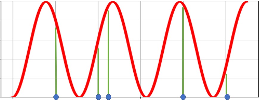
Figure 1: Sine fitting. Given a set of integers $P$ (blue points on the $x$-axis), and $\sin^{2}(\cdot)$ wave (the red signal), then the cost of the Sine fitting problem with respect to this input, is the sum of vertical distances between the points in $P$ (on the x-axis) and the sine signal (the sum of lengths of the green lines). The goal is to find the sine signal that minimizes this sum.

Formally speaking, the anomaly detection problem can be stated as follows. Given a large positive number $N$, a set $P\subseteq\left\{1,2,\cdots,N\right\}$ of $n$ integers, the objective is to fit a sine signal, such that the sum of the vertical distances between each $p\in P$ (on the $x$-axis) and its corresponding point $\sin^{2}\left(\frac{2\pi}{N}pc\right)$ on the signal, is minimized; see Figure 1. Hence, we aim to solve the following problem that we call the Sine fitting problem:

$$\begin{split}\min_{c\in C}\sum\limits_{p\in P}\sin^{2}\left(\frac{2\pi}{N}pc\right)+\lambda(c),\end{split}$$ (1)

where $C$ is the set of feasible solutions, and $\lambda$ is a regularization function to put constraints on the solution.

The generalized form of the fitting problem above was first addressed by Souders et al., (1994) and later generalized by Ramos and Serra, (2008), where proper implementation have been suggested over the years da Silva and Serra, (2003); Chen et al., (2015); Renczes et al., (2016); Renczes and Pálfi, (2021). In addition, the Sine fitting problem and its variants gained attention in recent years in solving various problems, e.g., estimating the shift phase between two signal with very high accuracy Queiros et al., (2010), characterizing data acquisition channels and analog to digital converters Pintelon and Schoukens, (1996), high-accuracy sampling measurements of complex voltage ratio of sinusoidal signals Augustyn and Kampik, (2018), etc.

Data discretization. In many applications, we aim to find a proper choice of floating-point grid. For example, when we are given points encoded in $64$bits, and we wish to use a $32$ floating point grid. A naive way to do so is by simply removing the most/least significant $32$ bits from each point. However such approach results in losing most of the underlying structure that these points form, which in turn leads to unnecessary data loss. Instead, arithmetic modulo or sine functions that incorporate cyclic properties are used, e.g., Naumov et al., (2018); Nagel et al., (2020); Gholami et al., (2021). Such functions aim towards retaining as much information as possible when information loss is inevitable. This task serves well in the field of quantization Gholami et al., (2021), which is an active sub-field in deep learning models.

To solve this problem, we first find the sine wave that fits the input data using the cost function at (1). Then each point in the input data is projected to its nearest point from the set of roots of the signal that was obtained from the sine fitting operation; see Figure 2.

All of the applications above, e.g., monitoring, anomaly detection, and data discretization, are problems that are reduced to an instance of the Sine fitting problem. Although these problems are desirable, solving them on large-scale data is not an easy task, due to bounded computational power and memory. In addition, in the streaming (or distributed) setting where points are being received via a stream of data, fitting such functions requires new algorithms for handling such settings. To handle these challenges, we can use coresets.

1.1 Coresets

Coreset was first suggested as a data summarization technique in the context of computational geometry (Agarwal et al.,, 2004), and got increasing attention over recent years (Broder et al.,, 2014; Tukan et al.,, 2020; Huang et al.,, 2021; Cohen-Addad et al.,, 2021; Huang et al.,, 2020; Mirzasoleiman et al.,, 2020); for extensive surveys on coresets, we refer the reader to (Feldman,, 2020; Phillips,, 2016), and Jubran et al., (2019); Maalouf et al., 2021b for an introductory.

Informally speaking, a coreset is (usually) a small weighted subset of the original input set of points that approximates its loss for every feasible query $c$, up to a provable multiplicative error of $1\pm\varepsilon$, where $\varepsilon\in(0,1)$ is a given error parameter. Usually the goal is to have a coreset of size that is independent or near-logarithmic in the size of the input (number of points), in order to be able to store a data of the same structure (as the input) using small memory, and to obtain a faster time solutions (approximations) by running them on the coreset instead of the original data. Furthermore, the accuracy of existing (fast) heuristics can be improved by running them many times on the coreset in the time it takes for a single run on the original (big) dataset. Finally, since coresets are designed to approximate the cost of every feasible query, it can be used to solve constraint optimization problems, and to support streaming and distributed models; see details and more advantages of coresets in (Feldman,, 2020).

In the recent years, coresets were applied to improve many algorithms from different fields e.g. logistic regression (Huggins et al.,, 2016; Munteanu et al.,, 2018; Karnin and Liberty,, 2019; Tukan et al.,, 2020), matrix approximation (Feldman et al.,, 2013; Maalouf et al.,, 2019; Feldman et al.,, 2010; Sarlos,, 2006; Maalouf et al., 2021c, ), decision trees (Jubran et al.,, 2021), clustering (Feldman et al.,, 2011; Gu,, 2012; Lucic et al.,, 2016; Bachem et al.,, 2018; Jubran et al.,, 2020; Schmidt et al.,, 2019), $\ell_{z}$-regression (Cohen and Peng,, 2015; Dasgupta et al.,, 2009; Sohler and Woodruff,, 2011), SVM (Har-Peled et al.,, 2007; Tsang et al.,, 2006; Tsang et al., 2005a, ; Tsang et al., 2005b, ; Tukan et al., 2021a, ), deep learning models (Baykal et al.,, 2018; Maalouf et al., 2021a, ; Liebenwein et al.,, 2019; Mussay et al.,, 2021), etc.

Sensitivity sampling framework. A unified framework for computing coresets to wide range family of problems was suggested in (Braverman et al.,, 2016). It is based on non-uniform sampling, specifically, sensitivity sampling. Intuitively, the sensitivity of a point $p$ from the input set $P$ is a number $s(p)\in[0,1]$ that corresponds to the importance of this point with respect to the other points, and the specific cost function that we wish to approximate; see formal details in Theorem 2. The main goal of defining a sensitivity is that with high probability, a non-uniform sampling from $P$ based on these sensitivities yields a coreset, where each point $p$ is sampled i.i.d. with a probability that is proportional to $s(p)$, and assigned a (multiplicative) weight which is inversely proportional to $s(p)$. The size of the coreset is then proportional to (i) the total sum of these sensitivities $t=\sum_{p\in P}s(p)$, and (ii) the VC dimension of the problem at hand, which is (intuitively) a complexity measure. In recent years, many classical and hard machine learning problems (Braverman et al.,, 2016; Sohler and Woodruff,, 2018; Maalouf et al., 2020b, ) have been proved to have a total sensitivity (and VC dimension) that is near-logarithmic in or even independent of the input size $\left|P\right|$.

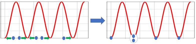
Figure 2: Discretization. Given a set of points (blue points), we find a sine wave (red signal) that fits the input data. Then each input point is projected to its nearest point from the set of roots of the signal.

1.2 Our Contribution

We summarize our contribution as follows.

1. Theoretically, we prove that for every integer $N>1$, and every set $P\subseteq[N]$ of $n>1$ integers:

   1. The total sensitivity with respect to the Sine fitting problem is bounded by $O(\log^{4}{N})$, and the VC dimension is bounded by $O(\log{(nN)})$; see Theorem 4 and Claim 12 respectively.

   2. For any approximation error $\varepsilon>1$, there exists a coreset of size $\tilde{O}\left(\log(N)^{O(1)}\right)$ (see Theorem 3 for full details) with respect to the Sine fitting optimization problem.

2. Experimental results on real world datasets and open source code (Code,, 2022) are provided.

2 PRELIMINARIES

In this section we first give our notations that will be used throughout the paper. We then define the sensitivity of a point in the context of the Sine fitting problem (see Definition 1), and formally write how it can be used to construct a coreset (see Theorem 2). Finally we state the main goal of the paper.

Notations. Let $\mathbb{Z}^{+}$ denote the set of all positive integers, $[n]=\left\{1,\ldots,n\right\}$ for every $n\in\mathbb{Z}^{+}$, and for every $x\in\mathbb{R}$ denote the rounding of $x$ to its nearest integer by $\left\lfloor x\right\rceil$ (e.g. $\left\lfloor 3.2\right\rceil=3$).

We now formally define the sensitivity of a point $p\in P$ in the context of the Sine fitting problem.

Definition 1 (Sine fitting sensitivity).

Let $N>1$ be a positive integer, and let $P\subseteq[N]$ be a set of $n>1$ integers. For every $p\in P$, the sensitivity of $p$ is defined as $\max_{c\in[N]}\frac{\sin^{2}(pc\cdot\frac{2\pi}{N})}{\sum_{q\in P}\sin^{2}(qc\cdot\frac{2\pi}{N})}.$

The following theorem formally describes how to construct an $\varepsilon$-coreset via the sensitivity framework. We restate it from Braverman et al., (2016) and modify it to be specific for our cost function.

Theorem 2.

Let $N>1$ be a positive integer, and let $P\subseteq[N]$ be a set of $n>1$ integers. Let $s:P\to[0,1]$ be a function such that $s(p)$ is an upper bound on the sensitivity of $p$ (see Definition 1). Let $t=\sum_{p\in P}s(p)$ and $d^{\prime}$ be the VC dimension of the Sine fitting problem; see Definition 11. Let $\varepsilon,\delta\in(0,1)$, and let $S$ be a random sample of $\left|S\right|\in O\left(\frac{t}{\varepsilon^{2}}\left(d^{\prime}\log{t}+\log{\frac{1}{\delta}}\right)\right)$ i.i.d points from $P$, where every $p\in P$ is sampled with probability $s(p)/t$. Let $v(p)=\frac{t}{s(p)\left|S\right|}$ for every $p\in S$. Then with probability at least $1-\delta$, we have that for every $c\in[N]$, we have $\left|1-\frac{\sum_{p\in S}v(p)\sin^{2}(pc\cdot\frac{2\pi}{N})}{\sum_{p\in P}\sin^{2}(pc\cdot\frac{2\pi}{N})}\right|\leq\varepsilon.$

Problem statement. Theorem 2 raises the following question: Can we bound the the total sensitivity and the VC dimension of the Sine fitting problem in order to obtain small coresets?

Note that, the emphasis of this work is on the size of the coreset that is needed (required memory) to approximate the Sine fitting cost function.

3 CORESET FOR SINE FITTING

In this section we state and prove our main result. For brevity purposes, some proofs of the technical results have been omitted from this manuscript; we refer the reader to the supplementary material for these proofs.

Note that since the regularization function $\lambda$ at (1) is independent of $P$, a $1\pm\varepsilon$ multiplicative approximation of the $\sin^{2}(\cdot)$ terms at (1), yields a $1\pm\varepsilon$ multiplicative approximation for the whole term in (1).

The following theorem summarizes our main result.

Theorem 3 (Main result: coreset for the Sine fitting problem).

Let $N>1$ be a positive integer, $P\subseteq[N]$ be a set of $n>1$ integers, and let $\varepsilon,\delta\in(0,1)$. Then, we can compute a pair $(S,v)$, where $S\subseteq P$, and $v:S\to[0,\infty)$, such that

1. the size of $S$ is polylogarithmic in $N$ and logarithmic in $n$, i.e.,

   $$|S|\in O\left(\frac{\log^{4}{N}}{\varepsilon^{2}}\left(\log(nN)\log{(\log{N})}+\log{\frac{1}{\delta}}\right)\right).$$

2. with probability at least $1-\delta$, for every $c\in[N]$,

   $$\left|1-\frac{\sum_{p\in S}v(p)\sin^{2}(pc\cdot\frac{2\pi}{N})}{\sum_{p\in P}\sin^{2}(pc\cdot\frac{2\pi}{N})}\right|\leq\varepsilon.$$

To prove Theorem 3, we need to bound the total sensitivity (as done in Section 3.1) and the VC dimension (see Section 3.2) of the Sine fitting problem.

3.1 Bound On The Total Sensitivity

In this section we show that the total sensitivity of the Sine fitting problem is small and bounded. Formally speaking,

Theorem 4.

Let $N\geq 1$ and $P\subseteq[N]$. Then

$$\sum_{p\in P}\max_{c\in[N]}\frac{\sin^{2}(pc\cdot\frac{2\pi}{N})}{\sum_{q\in P}\sin^{2}(qc\cdot\frac{2\pi}{N})}\in O(\log^{4}N).$$

We prove Theorem 4 by combining multiple claims and lemmas. We first state the following as a tool to use the cyclic property of the sine function.

Claim 5.

Let $a,b\in\mathbb{Z}^{+}$ be a pair of positive integers. Then for every $x\in\mathbb{Z}^{+}$,

$$\left|\sin{\left(\frac{b\pi}{a}x\right)}\right|=\left|\sin{\left(\frac{b\pi}{a}\left(x\ \mathrm{mod}\ a\right)\right)}\right|.$$

We now proceed to prove that one doesn’t need to go over all the possible integers in $[N]$ to compute a bound on the sensitivity of each $p\in P$, but rather a smaller compact subset of $[N]$ is sufficient.

Lemma 6.

Let $P\subseteq[N]$ be a set of $n$ integer points. For every $p\in P$, let

$$C(p)=\left\{c\in[N]\middle|\left(cp\ \mathrm{mod}\ \frac{N}{2}\right)\in\left[\frac{N}{8},\frac{3N}{8}\right]\right\}.$$

Then for every $p\in P$,

$$\max_{c\in[N]}\frac{\sin^{2}\left(\frac{2\pi}{N}pc\right)}{\sum\limits_{q\in P}\sin^{2}\left(\frac{2\pi}{N}qc\right)}\leq 4\cdot\max\limits_{c\in C(p)}\frac{\sin^{2}\left(\frac{2\pi}{N}pc\right)}{\sum\limits_{q\in P}\sin^{2}\left(\frac{2\pi}{N}qc\right)}.$$ (2)

Proof.

Put $p\in P$, and let $c^{*}\in[N]$ be an integer that maximizes the left hand side of (2) with respect to $p$, i.e.,

$$\max_{c\in[N]}\frac{\sin^{2}\left(pc\cdot\frac{2\pi}{N}\right)}{\sum_{q\in P}\sin^{2}\left(qc\cdot\frac{2\pi}{N}\right)}=\frac{\sin^{2}\left(pc^{*}\cdot\frac{2\pi}{N}\right)}{\sum_{q\in P}\sin^{2}\left(qc^{*}\cdot\frac{2\pi}{N}\right)}.$$ (3)

If $c^{*}\in C(p)$ the claim trivially holds. Otherwise, we have $c^{*}\in[N]\setminus C(p)$, and we prove the claim using case analysis: Case (i) $(c^{*}p\ \mathrm{mod}\ \frac{N}{2})\in\left[0,\frac{N}{8}\right)$, and Case (ii) $(c^{*}p\ \mathrm{mod}\ \frac{N}{2})\in\left(\frac{N}{2}-\frac{N}{8},\frac{N}{2}\right]$.

Case (i): Let $b_{2}\in[8]\setminus[3]$ be an integer, and let $z=\left\lceil\frac{N/b_{2}}{c^{*}p\ \mathrm{mod}\ \frac{N}{2}}\right\rceil$. We first observe that

$$\begin{split}z&=\left\lceil\frac{\frac{N}{b_{2}}}{c^{*}p\ \mathrm{mod}\ \frac{N}{2}}\right\rceil\\ &=\frac{\frac{N}{b_{2}}}{c^{*}p\ \mathrm{mod}\ \frac{N}{2}}+\frac{\left(-\frac{N}{b_{2}}\right)\ \mathrm{mod}\ \left(c^{*}p\ \mathrm{mod}\ \frac{N}{2}\right)}{c^{*}p\ \mathrm{mod}\ \frac{N}{2}},\end{split}$$ (4)

where the second equality hold by properties of the ceiling function. We further observe that,

$$\begin{split}&z\left(c^{*}p\ \mathrm{mod}\ \frac{N}{2}\right)\\ &=\frac{N}{b_{2}}+\left(-\frac{N}{b_{2}}\right)\ \mathrm{mod}\ \left(c^{*}p\ \mathrm{mod}\ \frac{N}{2}\right)\\ &\in\left[\frac{N}{b_{2}},\frac{N}{8}+\frac{N}{b_{2}}\right],\end{split}$$ (5)

where the first equality holds by expanding $z$ using (4), and the last inclusion holds by the assumption of Case (i). Since $\left[\frac{N}{b_{2}},\frac{N}{8}+\frac{N}{b_{2}}\right]$ is entirely included in $\left[\frac{N}{8},\frac{3N}{8}\right]$, then it holds that $z\left(c^{*}p\ \mathrm{mod}\ \frac{N}{2}\right)\in C(p)$. Similarly, one can show that $\left(zc^{*}p\right)\ \mathrm{mod}\ \frac{N}{2}\in\left[\frac{N}{b_{2}},\frac{N}{8}+\frac{N}{b_{2}}\right]$, which means that $zc^{*}\in C(p)$.

We now proceed to show that the sensitivity can be bounded using some point in $C(p)$. Since for every $x\in\left[0,\frac{\pi}{2}\right]$, $\sin{x}\leq x\leq 2\left|\sin{x}\right|$, then it holds that

$$\begin{split}&\sin^{2}\left(\frac{2\pi}{N}pc^{*}\right)=\sin^{2}\left(\frac{2\pi}{N}\left(c^{*}p\ \mathrm{mod}\ \frac{N}{2}\right)\right)\\ &\leq\left(\frac{2\pi}{N}\left(c^{*}p\ \mathrm{mod}\ \frac{N}{2}\right)\right)^{2}\\ &=\left(\frac{2\pi}{N}z\left(c^{*}p\ \mathrm{mod}\ \frac{N}{2}\right)\right)^{2}\frac{1}{z^{2}}\\ &\leq\frac{4}{z^{2}}\sin^{2}\left(\frac{2\pi}{N}z\left(c^{*}p\ \mathrm{mod}\ \frac{N}{2}\right)\right)\\ &=\frac{4}{z^{2}}\sin^{2}\left(\frac{2\pi}{N}zc^{*}p\right),\end{split}$$ (6)

where the first equality holds by plugging $a:=\frac{N}{2}$, $b:=1$ and $x:=c^{*}p$ into Claim 5, the first inequality holds since $\frac{2\pi}{N}\left(c^{*}p\ \mathrm{mod}\ \frac{N}{2}\right)\in[0,\pi]$, the second equality holds by multiplying and dividing by $z$, the second inequality follows from combining the fact that $\frac{2\pi}{N}z\left(c^{*}p\ \mathrm{mod}\ \frac{N}{2}\right)\leq\frac{\pi}{4}+\frac{\pi}{b_{2}}\leq\pi$ which is derived from (5) and the observation that $2\left|\sin{x}\right|\geq x$ for every $x\in\left[0,\frac{\pi}{2}\right]$, and the last equality holds by plugging $a:=\frac{N}{2}$, $b:=z$ and $x:=c^{*}p$ into Claim 5.

In addition, it holds that for every $q\in P$

$$\begin{split}&\sin^{2}\left(\frac{2\pi}{N}\left(c^{*}q\ \mathrm{mod}\ \frac{N}{2}\right)\right)\\ &\quad\geq\frac{1}{4}\left(\frac{2\pi}{N}\left(c^{*}q\ \mathrm{mod}\ \frac{N}{2}\right)\right)^{2}\\ &\quad=\frac{\left(\frac{2z\pi}{N}\left(c^{*}q\ \mathrm{mod}\ \frac{N}{2}\right)\right)^{2}}{4z^{2}}\\ &\quad\geq\frac{\sin^{2}\left(\frac{2z\pi}{N}\left(c^{*}q\ \mathrm{mod}\ \frac{N}{2}\right)\right)}{4z^{2}}\\ &\quad=\frac{1}{4z^{2}}\sin^{2}\left(\frac{2\pi}{N}zc^{*}q\right),\end{split}$$ (7)

where the first inequality holds by combining the assumption of Case (i) and the observation that $\left|\sin{x}\right|\geq\frac{x}{2}$ for every $x\in\left[0,\frac{\pi}{2}\right]$, the first equality holds by multiplying and dividing by $z$, the second inequality holds by combining (5) with the observation that $x\geq\left|\sin{x}\right|$ for every $x\in[0,\pi)$ where in this context $x:=\frac{2z\pi}{N}\left(c^{*}q\ \mathrm{mod}\ \frac{N}{2}\right)$, and finally the last equality holds by plugging $a:=\frac{N}{2}$, $b:=z\pi$, and $x:=c^{*}q$ into Claim 5.

Combining (3), (5), (6) and (7) yields that

$$\begin{split}&\max_{c\in[N]}\frac{\sin^{2}\left(\frac{2\pi}{N}pc\right)}{\sum\limits_{q\in P}\sin^{2}\left(\frac{2\pi}{N}qc\right)}\\ &\leq\max_{c\in[N]}\frac{\frac{16}{z^{2}}\sin^{2}\left(\frac{2\pi z}{N}\left(pc\ \mathrm{mod}\ \frac{N}{2}\right)\right)}{\frac{1}{z^{2}}\sum\limits_{q\in P}\sin^{2}\left(\frac{2\pi z}{N}\left(qc\ \mathrm{mod}\ \frac{N}{2}\right)\right)}\\ &=\max_{c\in[N]}\frac{16\sin^{2}\left(\frac{2\pi}{N}zpc\right)}{\sum_{q\in P}\sin^{2}\left(\frac{2\pi}{N}zqc\right)}=\max_{\hat{c}\in C(p)}\frac{16\sin^{2}\left(\frac{2\pi}{N}\hat{c}p\right)}{\sum_{q\in P}\sin^{2}\left(\frac{2\pi}{N}\hat{c}q\right)},\end{split}$$

where last equality holds from combining (3) and $zc^{*}\in C(p)$.

Case (ii): Let $c^{\prime}=N-c^{*}$, and note that $c^{\prime}\in[N]$. For every $q\in P$,

$$\left|\sin\left(c^{\prime}q\cdot 2\pi/N\right)\right|=\left|\sin\left(c^{*}q\cdot 2\pi/N\right)\right|.$$

We observe that

$$(c^{\prime}p\ \mathrm{mod}\ \frac{N}{2})=(N-c^{*})p\ \mathrm{mod}\ \frac{N}{2}$$

$$\quad\quad=\left(Np\ \mathrm{mod}\ \frac{N}{2}+(-c^{*}p)\ \mathrm{mod}\ \frac{N}{2}\right)\ \mathrm{mod}\ \frac{N}{2}$$

$$\quad\quad=\left(0+(-c^{*}p)\ \mathrm{mod}\ \frac{N}{2}\right)\ \mathrm{mod}\ \frac{N}{2}$$

$$\quad\quad=(-c^{*}p)\ \mathrm{mod}\ \frac{N}{2}$$

$$\quad\quad\leq-\left(N/2-N/8\right)\ \mathrm{mod}\ \frac{N}{2}$$

$$\quad\quad=N/8\ \mathrm{mod}\ \frac{N}{2}-N\ \mathrm{mod}\ \frac{N}{2}=N/8.$$

Hence, the proof of Claim 6 in Case (ii) follows by replacing $c^{*}$ with $c^{\prime}$ in Case (i). ∎

In what follows, we show that the sensitivity of each point $p\in P$ is bounded from above by a factor that is proportionally polylogarithmic in $N$ and inversely linear in the number of points $q\in P$ that are not that far from $p$ in terms of arithmetic modulo.

Lemma 7.

Let $C(p)$ be as in Lemma 6 for every $p\in P$, and let

$$\begin{split}g(p,P)&=\min_{c\in C(p)}\left|\left\{q\in P:(cq\ \mathrm{mod}\ \frac{N}{2})\in\right.\right.\\ &\left.\left.\left[\frac{N}{16\log N},\frac{N}{2}-\frac{N}{16\log N}\right]\right\}\right|.\end{split}$$ (8)

Then for every $p\in P$,

$$\max_{c\in C(p)}\frac{\sin^{2}\left(pc\cdot\frac{2\pi}{N}\right)}{\sum_{q\in P}\sin^{2}\left(qc\cdot\frac{2\pi}{N}\right)}\in O(\log^{2}N)\cdot\frac{1}{g(p,P)}.$$

Proof.

Put $p\in P$, $c\in C(p)$, and let $P^{\prime}=\left\{q\in P:\sin^{2}\left(qc\cdot\frac{2\pi}{N}\right)\geq 1/(8\log{N})^{2}\right\}$.

First we observe that for every $q\in P$ such that $\sin^{2}\left(qc\cdot\frac{2\pi}{N}\right)\geq 1/(8\log{N})^{2}$, it is implied that $(qc)\ \mathrm{mod}\ \frac{N}{2}\geq\frac{N}{16\log{N}}$. By the cyclic property of $\sin$, it holds that $(qc)\ \mathrm{mod}\ \frac{N}{2}\leq\frac{N}{2}-\frac{N}{16\log{N}}$.

Combining the above with the fact that $\sin^{2}\left(pc\cdot\frac{2\pi}{N}\right)\leq 1$, yields that

$$\begin{split}&\frac{\sin^{2}\left(pc\cdot\frac{2\pi}{N}\right)}{\sum_{q\in P}\sin^{2}\left(qc\cdot\frac{2\pi}{N}\right)}\\ &\quad\leq\frac{1}{\sum_{q\in P}\sin^{2}\left(qc\cdot\frac{2\pi}{N}\right)}\leq\frac{1}{\sum_{q\in P^{\prime}}\sin^{2}\left(qc\cdot\frac{2\pi}{N}\right)}\\ &\quad\leq\frac{1}{\left|P^{\prime}\right|/\left(64\log^{2}N\right)}\leq\frac{64\log^{2}N}{g(p,P)},\end{split}$$

where the second inequality follows from $P^{\prime}\subseteq P$, and the last derivation holds since $g(p,P)\leq\left|P^{\prime}\right|$ which follows from (8). ∎

The bound on the sensitivity of each point $p\in P$ (from the Lemma 7) still requires us to go over all possible queries in $C(p)$ to obtain the closest points in $P$ to $p$. Instead of trying to bound the sensitivity of each point by a term that doesn’t require evaluation over every query in $C(p)$, we will bound the total sensitivity in a term that is independent of $C(p)$ for every $p\in P$. This is done by reducing the problem to an instance of the expected size of independent set of vertices in a graph (see Claim 9). First, we will use the following claim to obtain an independent set of size polylogarithmic in the number of vertices in any given directed graph.

Claim 8.

Let $G$ be a directed graph with $n$ vertices. Let $d_{i}$ denote the out degree of the $i$th vertex, for $i=1,\cdots,n$. Then there is an independent set of vertices $Q$ in $G$ such that $|Q|\in\frac{\Theta(1)}{\log N}\cdot\sum_{i=1}^{n}\frac{1}{d_{i}+1}.$

Proof.

Let $V$ denote the set of vertices of $G$, and let $E$ denote the set of edges of $G$. Partition the vertices of $G$ into $O(\log n)$ induced sub-graphs, where each vertex in the $j$th sub-graph $H_{j}$ has out degree in $[2^{j-1},2^{j}-1]$ for any non-negative integer $j\leq\left\lfloor\log{\left(\max\limits_{i\in[n]}d_{i}\right)}\right\rceil$. Let $H$ denote the sub-graph with the largest number of vertices. Pick a random sample $S$ of $|V|^{2}/(2|E|)$ nodes from $V$. The expected number of edges in the induced sub-graph of $H$ by $S$ is bounded by $|V|^{2}/(4|E|)$. Let

$$T= \{v\mid(v,u)\text{ is an edge of the sub-graph of }H$$

$$\text{ induced by }S\}.$$

By Markov inequality, with probability at least $1/2$ we have $|T|\leq V^{2}/2$. Assume that this event indeed holds. Hence, the sub-graph of $H$ that is induced by $S\setminus T$ is an independent set of $H$ with $|S\setminus T|=|V|^{2}/2|E|-V^{2}/4|E|\geq V^{2}/4|E|$ nodes. Since $|E|\in O\left(2^{j}\left|V\right|\right)$ we have $|S_{j}\setminus T_{j}|=|V|/2^{j}\in\sum_{v\in V_{j}}\Theta(1)/d_{v}$. Hence, $\sum_{j}\left|S_{j}\setminus T_{j}\right|\in\sum_{v\in V}\Theta(1)/d_{v}$. By the pigeonhole principle, there is $j$ such that $\left|S_{j}\setminus T_{j}\right|$ can be bounded from below by $\sum_{v\in V}\Theta(1)/d_{v}/O(\log n)$. ∎

Claim 9.

There is a set $Q\subseteq P$ such that $g(q,Q)=1$ for every $q\in Q$, and $\sum_{p\in P}\frac{1}{g(p,P)}\in|Q|\cdot\Theta\left(\log N\right).$

Proof.

Let $b_{2}$ be defined as in the proof of Lemma 6. For every $p\in P$, let $g^{-1}(p,P)\in C(p)$ such that

$$g^{-1}(p,P)\in$$

$$\quad\arg\min_{c\in C(p)}\left|\left\{q\in P\setminus{\left\{p\right\}}:\sin^{2}\left(qc\cdot\frac{2\pi}{N}\right)\geq\frac{b2}{N}\right\}\right|.$$

Let $G=(P,E)$ denote the directed graph whose vertices are the integers in $P$, and whose edges are

$$\begin{split}E&:=\bigg{\{}(p,q)\in P\times P:p\neq q\text{ and }\\ &\sin^{2}\left(\frac{2\pi}{N}qg^{-1}(p,P)\right)\geq\frac{1}{b_{3}}\bigg{\}}.\end{split}$$ (9)

The out degree of a vertex $p$ of $G$ is $g(p,P)-1$. By Claim 8, there is independent set $Q$ of $G$ such that $\sum_{i=1}^{n}\frac{1}{g(p,P)}\in|Q|\cdot\Theta(\log N).$ Since $Q$ is independent set, for every $q\in Q$ we have $g(q,Q)=1$. ∎

The following claim serves to bound the size of the independent set, i.e., for every point $p\in P$ in the set, $g(p,P)=1$.

Claim 10.

Let $Q\subseteq[N]$ such that $g(q,Q)=1$ for every $q\in Q$. Then $|Q|\leq\log N.$

Finally, combining Lemma 6, Lemma 7, Claim 9 and Claim 10, satisfies Theorem 4 which presents a bound on the total sensitivity with respect to the $\sin^{2}\left(\cdot\right)$ cost function.

3.2 Bound on The VC Dimension

First, we define VC dimension with respect to the Sine fitting problem.

Definition 11 (VC-dimension (Braverman et al.,, 2016)).

Let $N>1$ be a positive integer, $P\subset[N]$ be a set of $n$ integer, and let $r\in[0,\infty)$, we define

$$\mathrm{ranges}(x,r)=\left\{p\in P\mid f(p,x)\leq r\right\},$$

for every $x\in[N]$ and $r\geq 0$. The dimension of the Sine fitting problem is the size $\left|S\right|$ of the largest subset $S\subset P$ such that

$$\left|\left\{S\cap\mathrm{ranges}(x,r)\mid x\in[N],r\geq 0\right\}\right|=2^{\left|S\right|}.$$

Lemma 12 (Bound on the VC dimension of the Sine fitting problem).

Let $n,N\geq 1$ be a pair of positive integers such that $n\leq N$, and let $P\subseteq[N]$ be a set of $n$ points. Then the VC dimension of the Sine fitting problem with respect to $P$ and $N$ is $O\left(\log\left(nN\right)\right)$.

Proof.

We note that the VC-dimension of the set of classifiers that output the sign of a sine wave parametrized by a single parameter (the angular frequency of the sine wave) is infinite. However since our query space is bounded, i.e., every query is an integer in the range $[1,N]$, then the VC dimension is bounded as follows. First, let $D(p,x)=\sin^{2}(px\cdot\frac{2\pi}{N})$ for every $p\in P$, and $x\in[n]$. We observe that for every $p\in P$ and $x\in[N]$, $D(p,x)\leq 1$. Hence, for every $x\in[N]$ and $r\in[0,\infty)$ it holds that $\left\{\mathrm{ranges}(x,r)\middle|r\geq 0\right\}=\left\{\mathrm{ranges}(x,r)\middle|r\in[0,1]\right\},$ where $\mathrm{ranges}(x,r)=\left\{p\in P\mid d(p,x)\leq r\right\}$ is defined as in Definition 11. Secondly, by the definition of $\mathrm{ranges}$, we have that for every pair of $r_{1},r_{2}\in[0,1]$ and $x\in[N]$ where $r_{2}\geq r_{1}$, $\mathrm{ranges}\left(x,r_{2}\right)=\bigcup\limits_{r\in\left[r_{1},r_{2}\right]}\mathrm{ranges}\left(x,r\right).$

This yields that $\left|\left\{\mathrm{ranges}\left(x,r\right)\middle|r\in[0,1]\right\}\right|\leq n$ for any $x\in[N]$, which consequently means that $\left|\left\{\mathrm{ranges}\left(x,r\right)\middle|x\in[N],r\geq 0\right\}\right|=nN,$ since $x\in[N]$ is an integer, and each such $x$ would create a different set of $n$ subsets of $P$. Thus we get that $\forall\,S\subseteq P$: $\left|\left\{S\cap\mathrm{ranges}\left(x,r\right)\middle|x\in[N],r\geq 0\right\}\right|\leq nN=2^{\log\left(nN\right)}.$

The claim then follows since the above inequality states that the VC dimension is bounded from above by $\log\left(nN\right)$. ∎

4 REMARKS AND EXTENSIONS

In this section briefly discuss several remarks and extensions of our work.

Parallel implementation. Computing the sensitivities for $n$ input points requires $O(Nn)$ time, this is by computing $cost(c):={\sum_{q\in P}\sin^{2}(qc\cdot\frac{2\pi}{N})}$ for every $c\in[n]$, and then bounding the sensitivity for very $p\in P$ by iterating over all queries $c\in[N]$, and taking the one which maximizes its term. However, this can be practically improved by applying a distributed fashion algorithm. Notably, one can compute the cost ${\sum_{q\in P}\sin^{2}\left(qc\cdot\frac{2\pi}{N}\right)}$ of every query $c\in[N]$ independently from all other queries in $[N]$, similarly, once we computed the cost of every query $c\in[N]$, the sensitivity of each point $p\in P$ can be computed independently from all of the other points. Algorithm 1 utilises these observations: It receives as input an integer $N$ which indicates the query set range, a set $P\subset[N]$, and an integer $M$ indicating the number of machines given to apply the computations on. Algorithm 1 outputs a function $s:P\to(0,\infty)$, where $s(p)$ is the sensitivity of $p$ for every $p\in P$.

Input : An integer $N>1$, a set $P\subset[N]$ of $n>1$ integers, and an integer $M\geq 1$.

Output : A function $s:P\to(0,\infty)$, where for every $p\in P:$ $s(p)$ is the sensitivity of $p$.

1

2$C_{1},\cdots,C_{M}:=$ a partition of $[N]$ into $M$ disjoint subsets, each contains at most $\left\lceil N/M\right\rceil$ integers from $[N]$. {In some cases, the last set $C_{M}$ might be empty.}

3$P_{1},\cdots,P_{M}:=$ a partition of $P$ into $M$ disjoint subsets, each contains at most $\left\lceil n/M\right\rceil$ integers from $P$. {In some cases, the last set $P_{M}$ might be empty.}

4for every $i\in[M]$, in distributed manner do

5      

6      for every $c\in C_{i}$ do

7            

8            Set $cost(c):={\sum_{q\in P}\sin^{2}\left(qc\cdot\frac{2\pi}{N}\right)}$

9for every $i\in[M]$, in distributed manner do

10      

11      for every $p\in P_{i}$ do

12            

13            Set $s(p):=\max_{c\in[N]}\frac{\sin^{2}\left(pc\cdot\frac{2\pi}{N}\right)}{cost(c)}$

14return $s$

Algorithm 1 $\textsc{Calculate-Sensitivities}(P,N,M)$

Extension to high dimensional data. Our results can be easily extended to the case where (i) the points (of $P$) lie on a polynomial grid of resolution $\Delta>0$ of any dimension $d\geq 1$, and (ii) they are further assumed to be contained inside a ball of radius $N>0$. Note that, such assumptions are common in the coreset literature, e.g., coresets for protective clustering Edwards and Varadarajan, (2005), relu function Mussay et al., (2021), and logistic regression Tolochinsky and Feldman, (2018). The analysis with respect to the sensitivity can be directly extended, and the VC dimension is now bounded by $O\left(d\log\left(\frac{N}{d}\Delta n\right)\right)$. Both claims are detailed at Section B of the appendix.

Approximating the optimal solution via coresets. Let $N>1$ be an integer, $P\subset[N]$, and let $(S,v)$ be a coreset for $P$ as in Theorem 2. Let $p^{*}\in\arg\min_{c\in[N]}\sum_{p\in P}\sin^{2}(pc\cdot\frac{2\pi}{N})$ and $c^{*}\in\arg\min_{c\in[N]}\sum_{p\in S}v(p)\sin^{2}(pc\cdot\frac{2\pi}{N})$ be the optimal solutions on the input and its coreset, respectively, then $\sum_{p\in P}\sin^{2}(pc^{*}\cdot{2\pi}{N})\leq(1+\varepsilon)\sum_{p\in P}\sin^{2}(pp^{*}\cdot{2\pi}{N})$.

5 EXPERIMENTAL RESULTS

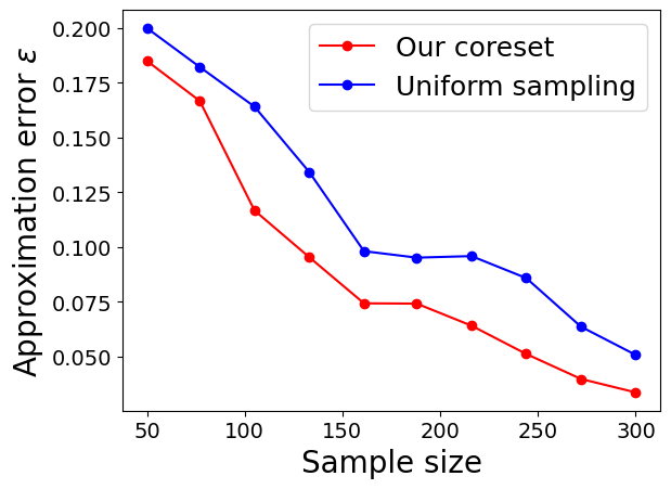
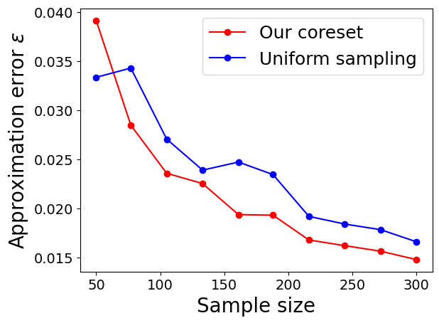
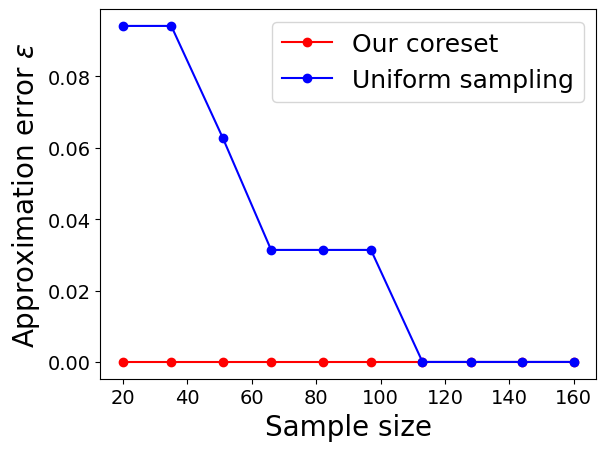
Figure 3: Optimal solution approximation error: The x axis is the size of the chosen subset, the y axis is the optimal solution approximation error. Datasets, from left to right, (i)-(1), (i)-(2), and (iii).

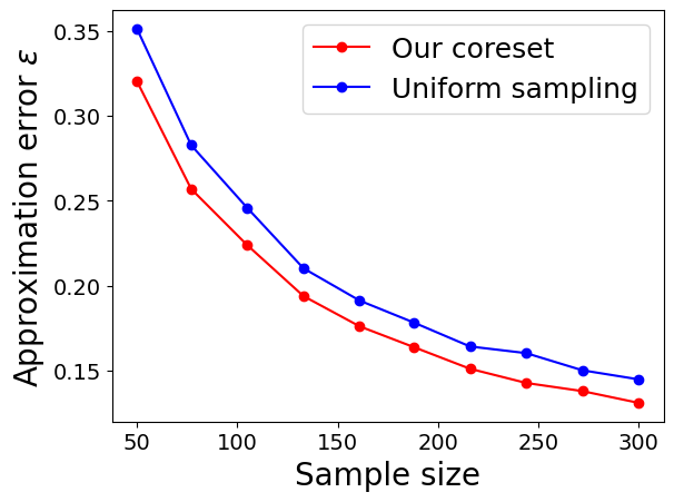
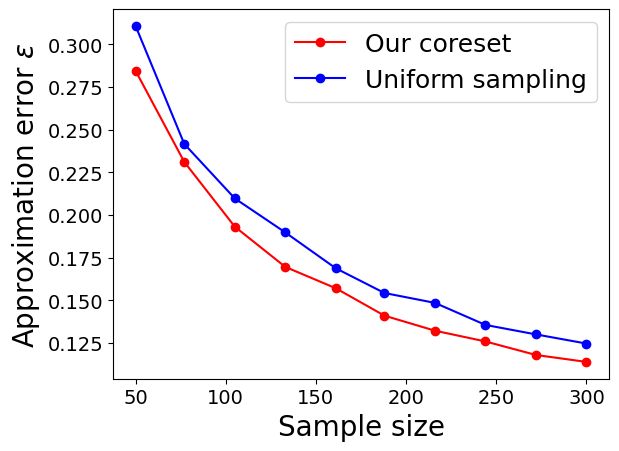
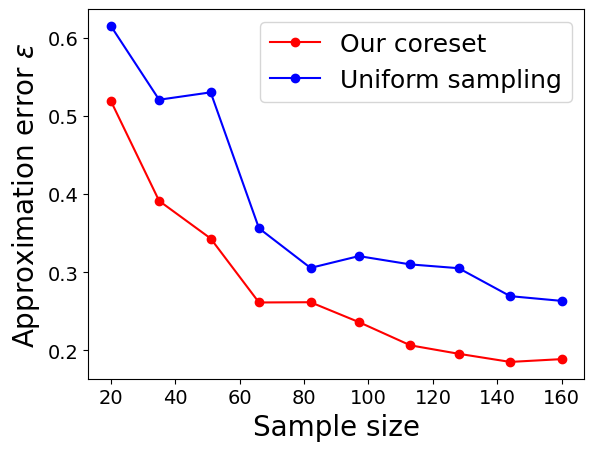
Figure 4: Maximum approximation error: The x axis is the size of the chosen subset, the y axis is the maximum approximation error across the whole set of queries. Datasets, from left to right, (i)-(1), (i)-(2), and (iii).

In what follows we evaluate our coreset against uniform sampling on real-world datasets.

Software/Hardware. Our algorithms were implemented in Python 3.6 (Van Rossum and Drake,, 2009) using “Numpy” (Oliphant,, 2006). Tests were performed on $2.59$GHz i$7$-$6500$U ($2$ cores total) machine with $16$GB RAM.

5.1 Datasets And Applications

1. Air Quality Data Set (De Vito et al.,, 2008), which contains $9,358$ instances of hourly averaged responses from an array of $5$ metal oxide chemical sensors embedded in an Air Quality Chemical Multisensor Device. We used two attributes (each as a separate dataset) of hourly averaged measurements of (1) tungsten oxide - labeled by (i)-(1) in the figures, and (2) NO2 concentration - labeled by (i)-(2). Fitting the sine function on each of these attributes aids in understanding their underlying structure over time. This helps us in finding anomalies that are far enough from the fitted sine function. Finding anomalies in this context could indicate a leakage of toxic gases. Hence, our aim is to monitor their behavior over time, while using low memory to store the data.

2. Single Neuron Recordings (Don H. Johnson, 2013b, ) acquired from a cat’s auditory-nerve fiber. The dataset has $127,505$ samples and the goal of Sine fitting with respect to such data is to infer cyclic properties from neuron signals which will aim in further understanding of the wave of a single neuron and it’s structure.

3. Dog Heart recordings of heart ECG (Don H. Johnson, 2013a, ). The dataset has $360,448$ samples. We have used the absolute values of each of the points corresponding to the “electrocardiogram” feature which refers to the ECG wave of the dog’s heart. The goal of Sine fitting on such data is to obtain the distribution of the heart beat rates. This aids to detects spikes, which could indicate health problems relating to the dog’s heart.

5.2 Reported Results

Approximation error. We iterate over different sample sizes, where at each sample size, we generate two coresets, the first is using uniform sampling and the latter is using sensitivity sampling. For every such coreset $(S,v)$, we compute and report the following.

1. The optimal solution approximation error, i.e., we find $c^{*}\in\arg\min_{c\in C}\sum_{p\in S}v(p)\sin^{2}(\frac{2\pi}{N}\cdot pc)$. Then the approximation error $\varepsilon$ is set to be $\frac{\sum_{p\in P}\sin^{2}(\frac{2\pi}{N}pc^{*})}{\min_{c\in C}\sum_{p\in P}\sin^{2}(\frac{2\pi}{N}pc)}-1$; see Figure 3.

2. The maximum approximation error of the coreset over all query in the query set, i.e., $\max_{c\in C}\left|1-\frac{\sum_{p\in S}v(p)\sin^{2}(\frac{2\pi}{N}pc)}{\sum_{p\in P}\sin^{2}(\frac{2\pi}{N}pc)}\right|$; see Figure 4.

The results were averaged across $32$ trials. As can be seen in Figures 3 and 4, the coreset in such context (for the described applications in Section 5.1) encapsulates the structure of the dataset and approximate the datasets behavior. Our coreset obtained consistent smaller approximation errors in almost all the experiments in both experiments than those obtained by uniform sampling. Observe that our advantage on Dataset (iii) is much more significant than the others as this dataset admits a clear periodic underlying structure. Note that, in some cases the coreset is able to encapsulate the entirety of the underlying structure at small sample sizes much better than uniform sampling due to its sensitivity sampling. This means that the optimal solution approximation error in practice can be zero; see the rightmost plot in Figure 3.

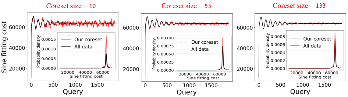
Figure 5: Sine fitting cost as a function of the given query. Dataset (ii) was used.

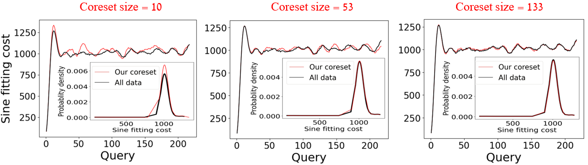
Figure 6: Sine fitting cost as a function of the given query. Dataset (iii) was used.

Approximating the Sine function’s shape and the probability density function of the costs. In this experiment, we visualize the Sine fitting cost as in (1) on the entire dataset over every query in $[N]$ as well as visualizing it on our coreset. As depicted in Figures 5 and 6, the large the coreset size, the smaller the deviation of both functions. This proves that in the context of Sine fitting , the coreset succeeds in retaining the structure of the data up to a provable approximation. In addition, due to the nature of our coreset construction scheme, we expect that the distribution will be approximated as well. This also can be seen in Figure 5 and 6. Specifically speaking, when the coreset size is small, then the deviation (i.e., approximation error) between the cost of (1) on the coreset from the cost of (1) on the whole data, will be large (theoretically and practically), with respect to any query in $[N]$. As the coreset size increases, the approximation error decreases as expected also in theory. This phenomenon is observed throughout our experiments, and specifically visualized at Figures 5 and 6 where one can see that the alignment between probability density functions with respect to the coreset and the whole data increases with the coreset size. Note that, we used only $2000$ points from Dataset (iii) to generate the results presented at Figure 6.

6 CONCLUSION, NOVELTY, AND FUTURE WORK

Conclusion. In this paper, we proved that for every integer $N>1$, and a set $P\subset[N]$ of $n>1$ integers, we can compute a coreset of size $O(\log(N)^{O(1)})$ for the Sine fitting problem as in (1). Such a coreset approximates the Sine fitting cost for every query $c$ up to a $1\pm\varepsilon$ multiplicative factor, allowing us to support streaming and distributed models. Furthermore, this result allows us to gain all the benefits of coresets (as explained in Section 1.1) while simultaneously maintaining the underlying structure that these input points form as we showed in our experimental results.

Novelty. The proofs are novel in the sense that the used techniques vary from different fields that where not previously leveraged in the context of coresets, e.g., graph theory, and trigonometry. Furthermore to our knowledge, our paper is the first to use sensitivity to obtain a coreset for problems where the involved cost function is trigonometric, and generally functions with cyclic properties. We hope that it will help open the door for more coresets in this field.

Future work includes (i) suggesting a coreset for a high dimensional input, (ii) computing and proving a lower bound on the time it takes to compute the coreset, (iii) extending our coreset construction to a generalized form of cost function as in (Souders et al.,, 1994; Ramos and Serra,, 2008), and (iv) discussing the applicability of such coresets in a larger context such as quantization (Hong et al.,, 2022; Zhou et al.,, 2018; Park et al.,, 2017) of deep neural networks while merging it with other compressing techniques such as pruning (Liebenwein et al.,, 2019; Baykal et al.,, 2018) and low-rank decomposition (Tukan et al., 2021b, ; Maalouf et al., 2020a, ; Liebenwein et al.,, 2021), and/or using it as a prepossessing step for other coreset construction algorithms that requires discretization constraints on the input, e.g., (Varadarajan and Xiao,, 2012).

7 ACKNOWLEDGEMENTS

This work was partially supported by the Israel National Cyber Directorate via the BIU Center for Applied Research in Cyber Security.

 

Supplementary Material:
Coresets for Data Discretization and Sine Wave Fitting

 

Appendix A PROOF OF TECHNICAL RESULTS

A.1 Proof of Claim 5

Proof.

Put $x\in\mathbb{Z}^{+}$ and observe that

$$x=\left\lfloor\frac{x}{a}\right\rfloor a+x\ \mathrm{mod}\ a.$$ (10)

Thus,

$$\begin{split}\left|\sin{\left(\frac{b\pi}{a}x\right)}\right|&=\left|\sin{\left(\frac{b\pi}{a}\left\lfloor\frac{x}{a}\right\rfloor a+\frac{b\pi}{a}x\ \mathrm{mod}\ a\right)}\right|\\ &=\left|\sin{\left(\left\lfloor\frac{x}{a}\right\rfloor b\pi+\frac{b\pi}{a}x\ \mathrm{mod}\ a\right)}\right|,\end{split}$$ (11)

where the first equality holds by (10).

Using trigonometric identities, we obtain that

$$\begin{split}&\left|\sin{\left(\left\lfloor\frac{x}{a}\right\rfloor b\pi+\frac{b\pi}{a}x\ \mathrm{mod}\ a\right)}\right|=\\ &\quad\left|\sin{\left(\left\lfloor\frac{x}{a}\right\rfloor b\pi\right)}\cdot\cos{\left(\frac{b\pi}{a}\left(x\ \mathrm{mod}\ a\right)\right)}\right.\\ &\quad\left.+\sin{\left(\frac{b\pi}{a}\left(x\ \mathrm{mod}\ a\right)\right)}\cdot\cos{\left(\left\lfloor\frac{x}{a}\right\rfloor b\pi\right)}\right|.\end{split}$$ (12)

Since $\left(\left\lfloor\frac{x}{a}\right\rfloor b\pi\right)\in\left\{0,\pi,2\pi,3\pi,\cdots\right\}$, we have that

$$\sin{\left(\left\lfloor\frac{x}{a}\right\rfloor b\pi\right)}=0,$$

and

$$\left|\cos{\left(\left\lfloor\frac{x}{a}\right\rfloor b\pi\right)}\right|=1.$$

By combining the previous equalities with (11) and (12), Claim 5 follows. ∎

A.2 Proof of Claim 10

Proof.

Contradictively assume that $|Q|\geq 1+\log N$, and let $T$ be a subset of $1+\log N$ integers from $Q$. Since $g(q,Q)=1$ for every $q\in Q$, we have

$$\left|\left\{q\ \mathrm{mod}\ \frac{N}{2}\right\}\right|=|Q|\geq 1+\log N.$$

Observer that (i) the set $T$ has $2^{|T|}>N$ different subsets. Hence it has $O(N^{2})$ distinct pair of subsets, and (ii) for any $T^{\prime}\subset T$ we have that $\sum_{q\in T^{\prime}}(q\ \mathrm{mod}\ \frac{N}{2})\in\left[\left\lfloor(1+\log N)\frac{N}{2}\right\rceil\right]$. By (i), (ii) and the pigeonhole principle there are two distinct sets $T_{1},T_{2}\subset T$ such that

$$\sum_{q\in T_{1}}(q\ \mathrm{mod}\ \frac{N}{2})=\sum_{q\in T_{2}}(q\ \mathrm{mod}\ \frac{N}{2}).$$

Put $p\in T_{2}$, and observe that

$$p\ \mathrm{mod}\ \frac{N}{2}=\sum_{q\in T_{1}}(q\ \mathrm{mod}\ \frac{N}{2})-\sum_{q\in T_{2}\setminus\left\{p\right\}}(q\ \mathrm{mod}\ \frac{N}{2}).$$

Therefore for every $c\in[N]$,

$$\begin{split}&cp\ \mathrm{mod}\ \frac{N}{2}=\quad c(p\ \mathrm{mod}\ \frac{N}{2}))\ \mathrm{mod}\ \frac{N}{2}\\ &=c\left(\sum_{q\in T_{1}}(q\ \mathrm{mod}\ \frac{N}{2})-\sum_{q\in T_{2}\setminus\left\{p\right\}}(q\ \mathrm{mod}\ \frac{N}{2})\right)\ \mathrm{mod}\ \frac{N}{2}\\ &\leq\left(\sum_{q\in T\setminus\left\{p\right\}}(cq\ \mathrm{mod}\ \frac{N}{2})\right)\ \mathrm{mod}\ \frac{N}{2}.\end{split}$$ (13)

Since $g(p,Q)=1$ by the assumption of the claim, there is $c\in C(p)$ such that for every $q\in T$ (where $q\neq p$), either (i) $cq\ \mathrm{mod}\ \frac{N}{2}\leq\frac{N}{16\log{N}}$, or, (ii) $cq\ \mathrm{mod}\ \frac{N}{2}\geq\frac{15N}{16\log{N}}$.

Handling Case (i). Assuming that this case holds, then by (13) we obtain that

$$\begin{split}cp\ \mathrm{mod}\ \frac{N}{2}&\leq\left(\sum\limits_{q\in T\setminus\left\{p\right\}}\frac{N}{16\log{N}}\right)\ \mathrm{mod}\ \frac{N}{2}\\ &=\frac{N}{16}\ \mathrm{mod}\ \frac{N}{2}=\frac{N}{16}.\end{split}$$

This contradicts the assumption that $c\in C(p)$.

Handling Case (ii). Combining the assumption of this case with (13), yields that

$$\begin{split}cp\ \mathrm{mod}\ \frac{N}{2}&\geq\left(\sum\limits_{q\in T\setminus\left\{p\right\}}\frac{15N}{16\log{N}}\right)\ \mathrm{mod}\ \frac{N}{2}\\ &=\frac{15N}{16}\ \mathrm{mod}\ \frac{N}{2}=\frac{15N}{16}.\end{split}$$

This is a contradiction to the assumption that $c\in C(p)$. ∎

Appendix B EXTENSION TO HIGH DIMENSIONAL DATA

In this section we formally discuss the generalization of our results to constructing coresets for sine fitting of rational high dimensional data. First note that in such (high dimensional) settings, the objective of the Sine fitting problem becomes

$$\min_{c\in C}\sum\limits_{p\in P}\sin^{2}\left(\frac{2\pi}{N}\cdot p^{T}c\right),$$

where $P$ is the set of high dimensional input points and $C$ is the set of queries. Note that, we still assume that both sets are finite and lie on a grid of resolution $\Delta$; see next paragraph for more details.

Assumptions.

To ensure the existence of coresets for the generalized form, we first generalize the assumptions of our results as follows: (i) the original set of queries $[N]$ is now generalized to be the set $B$ of all points with non-negative coordinates and of resolution $\Delta$. Formally speaking, let $\Delta>0$ be a rational number that denotes the resolution, and let $X:=\left\{i\Delta\right\}_{i=0}^{\left\lfloor\frac{N}{\sqrt{d}\Delta}\right\rfloor}\cup\left\{N/\sqrt{d}\right\}$ denote the set $\left\{0,\Delta,2\Delta,3\delta,\cdots,N/\sqrt{d}\right\}$, now, our set of queries is defined to be

$$B:=X^{d}=\underbrace{X\times X\times\cdots\times X}_{d\text{ times}},$$

i.e., $B\subset\mathbb{R}^{d}$, and for every $i\in[d]$ and $x\in B$, the $i$th coordinate $x_{i}$ of $x$ is from $X$ (if $x\in B$, then $\forall_{i\in[d]}x_{i}\in X$). (ii) The input $P$ is contained in the set of queries, thus, our generalization assumes that $P\subseteq B$.

Sensitivity bound and total sensitivity bound.

First, for every $x\in B$ and $p\in P$ let $D(p,x)=\sin^{2}\left(\frac{2\pi}{N}p^{T}x\right)$. The main reason that the our main result which suits the one dimensional setting (where points and queries are integers) is interesting, relies on the fact that each point $p$ in the input set $P$ results a sine wave $Sine(p,\cdot):[N]\to[0,1]$ of a different wavelengths, where specifically for a point $p\in P\subseteq[N]$, the wavelength of the corresponding sine wave is $\frac{2\pi p}{N}$. This ensures that most point don’t admit the same squared sine waves which in turn fuels the need to find a small set of points that the sum of their squared sine waves approximate the total sum of the squared sine waves of the input set of integral points in one dimensional space.

Following the same observation, we simply generalize our cost function to account for such traits, where the wavelength of the obtained signals is shown along the direction of the points in $P\subseteq B$; the following figure serves as descriptive illustration.

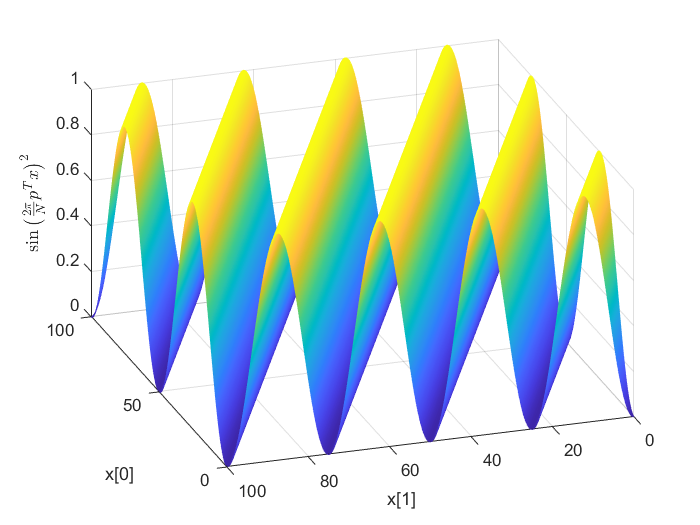
Figure 7: Given a point $p:=\begin{pmatrix}1\\ 2\end{pmatrix}$ and a set of queries $B$ where $\Delta:=0.1$ and $N=100$, the above is a plot of $\sin^{2}{\left(\frac{2\pi}{N}p^{T}x\right)}$ over every query $x\in B$. Here the $x$-axis denotes the first entry of a query $x\in B$, the $y$-axis denotes the second entry of a query $x$.

Following along the ideas above from the one dimensional case, choosing the set of queries to be $B$, and $P$ to be any set of $n$ points contained in $B$, fulfills the same ideas. Thus, we can use $D(p,x):=\sin^{2}{\left(\frac{2\pi}{N}p^{T}x\right)}$ as our generalized form of squared sine loss function.

Since the dot product is non-negative in our context, it behave as a generalization of the product between two non-negative scalars. Our previous results depends on the product of two scalars rather than the scalar themselves, and from such observation, it can be seen as a leverage point for this generalization to be equipped into our proofs.

Bounding the VC dimension.

It was stated previously that the necessity of generalizing the assumptions of our results is crucial. Such necessity is needed to handle the case of restricting the VC dimension of the Sine fitting problem in the $d$-dimensional Euclidean space to be finite. The following gives the formal ingredients for such purpose.

Lemma 13 (Extension of Lemma 12).

Let $N,n,d$ be a triplet of positive integers where $N\geq n>d$. Let $\Delta>0$ be rational number such that, let $X:=\left\{i\Delta\right\}_{i=0}^{\left\lfloor\frac{N}{\sqrt{d}\Delta}\right\rfloor}\cup\left\{\frac{N}{\sqrt{d}}\right\}$, and let $B:=X^{d}$ denote the set of all $d$-dimensional points such that each coordinate of any point $x\in B$ is from $X$, i.e., $B$ has a resolution of $\Delta$. Let $P\subseteq B$ be a set of $n$ points. Then the VC dimension of the Sine fitting problem with respect to $P$ and $B$ is $O\left(d\log\left(\frac{N}{\Delta}n\right)\right)$.

Proof.

The following proof relies on an intuitive generalization of the proof of Lemma 12. We note again that the VC-dimension of the set of classifiers that output the sign of a sine wave parametrized by a single parameter (the angular frequency of the sine wave) is infinite. Regardless, our query space is bounded, i.e., every query contained in a ball of radius $N$. Thus, we bound the VC dimension as follows. First let $D(p,x)=\sin^{2}\left(p^{T}\cdot x\frac{2\pi}{N}\right)$ we observe that for every $p\in P$ and $x\in B$, $D(p,x)\leq 1$. Hence, for every $x\in B$ and $r\in[0,\infty)$ it holds that

$$\left\{\mathrm{ranges}(x,r)\middle|r\geq 0\right\}=\left\{\mathrm{ranges}(x,r)\middle|r\in[0,1]\right\},$$

where $\mathrm{ranges}(x,r)=\left\{p\in P\mid D(p,x)\leq r\right\}$ is defined as in Definition 11. Secondly, by the definition of $\mathrm{ranges}$, we have that for every pair of $r_{1},r_{2}\in[0,1]$ and $x\in B$ where $r_{2}\geq r_{1}$, $\mathrm{ranges}\left(x,r_{2}\right)=\bigcup\limits_{r\in\left[r_{1},r_{2}\right]}\mathrm{ranges}\left(x,r\right).$

This yields that $\left|\left\{\mathrm{ranges}\left(x,r\right)\middle|r\in[0,1]\right\}\right|\leq n$ for any $x\in B$, which consequently means that

$$\left|\left\{\mathrm{ranges}\left(x,r\right)\middle|x\in B,r\geq 0\right\}\right|\leq n\left|B\right|,$$

since $x\in B$ is an integer, and each such $x$ would create a different set of $n$ subsets of $P$.

Since $B$ is contained in a ball of radius $N$, it holds that $\left|B\right|\in O\left(\frac{N^{d}}{\Delta^{d}}\right)$. We thus get that $\forall\,S\subseteq P$,

$$\left|\left\{S\cap\mathrm{ranges}\left(x,r\right)\middle|x\in[N],r\geq 0\right\}\right|\leq\frac{n}{\Delta^{d}}\mathrm{vol}\left(B\right)\in 2^{O\left(d\log\left(\frac{N}{\Delta}n\right)\right)}.$$

The lemma then follows since the above inequality states that the VC dimension is bounded from above by $O\left(d\log\left(\frac{N}{\Delta}n\right)\right)$. ∎

Appendix C ADDITIONAL EXPERIMENTS

In this section, we carry additional experiments to show the advantage of our method in comparison with uniform sampling. We note that Figure 8 is given to show that the heartbeat data Don H. Johnson, 2013a is not of the form of a a flat-like line with regular peaks. In what follows, we show additional experiments on with respect to the sine fitting problem and the data discretization problem. For such task, we consider the following dataset:

Bat Echoes (Don H. Johnson, 2013b, )

– acquired from the echolocation pulse emitted by the Large Brown Bat (Eptesicus Fuscus). Such a file has a duration of $2.8ms$ and was digitized by considering a sampling period of $7\mu s$, resulting in a file with $400$ samples.

At Figure 9, it is shown that our coreset clearly outperforms uniform sampling with respect to the Sine fitting problem.

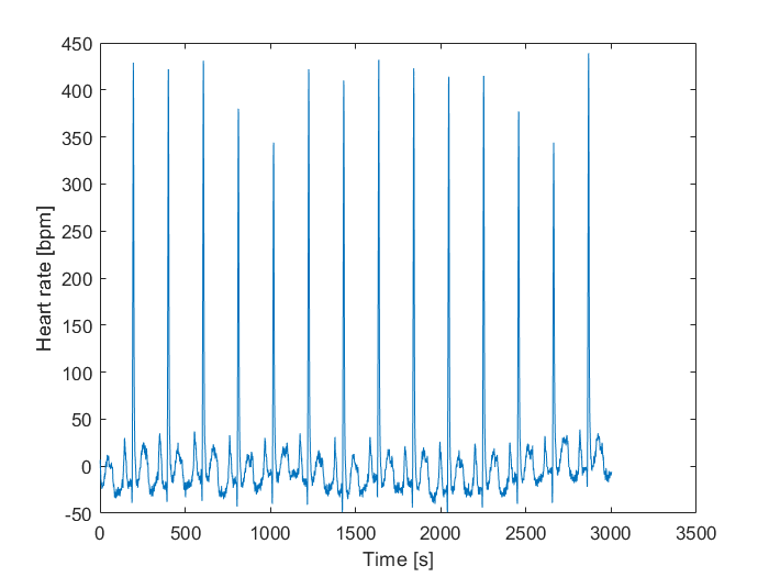
Figure 8: A snippet of the electrocardiogram with respect to a beating heart of some dog.

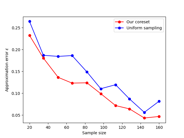
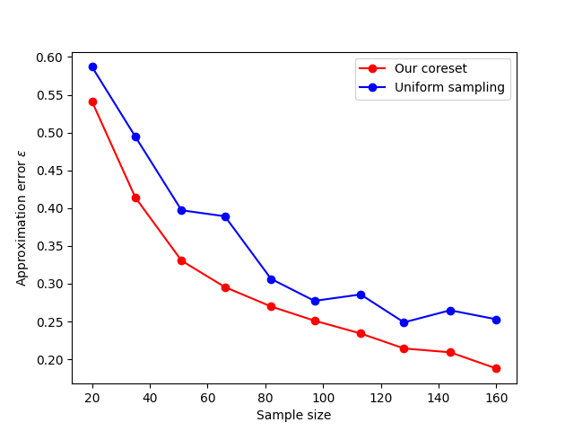
Figure 9: The optimal and maximal approximation errors with respect to the bat echoes dataset: The x axis is the size of the chosen subset, the y axis is the approximation error across the whole set of queries. The left figure shows the optimal solution approximation error, while the right figure serves to show the maximal approximation error across the whole set of queries.

We conclude this section with an experiment done to assess the effectiveness of our coreset against that of uniform sampling for the task of data discretization. Figure 10 shows the advantage of using our coreset upon using uniform sampling. For this experiment, the optimal solution of (1) with respect to each of the coreset and sampled set of points using uniform sampling is computed. Then using each of the solutions, we generate a sine waves such that its phase is equal to the computed solutions. We then project the points of the whole input data on the closest roots of these waves respectively, resulting into two sets of points. Now, we compute the distance between each point and its projected point and sum up the distance for each of the projected sets of points. Finally, we compute the approximated yielded by these values with respect to the value which we would have obtained if this process was done solely on the whole data.

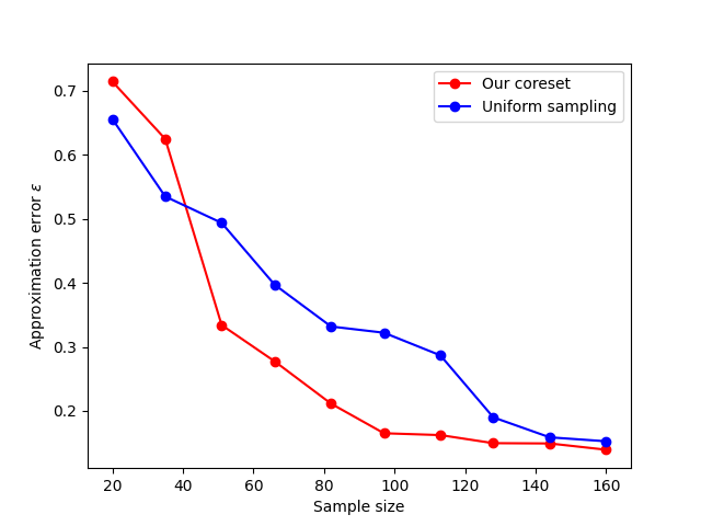
Figure 10: The optimal approximation error with respect to the bat echoes dataset: The x axis is the size of the chosen subset, the y axis is the approximation error across the whole set of queries. The left figure shows the optimal solution approximation error, while the right figure serves to show the maximal approximation error across the whole set of queries. This figure is with respect to the data discretization problem.

References

- Agarwal et al., (2004) Agarwal, P. K., Har-Peled, S., and Varadarajan, K. R. (2004). Approximating extent measures of points. Journal of the ACM (JACM), 51(4):606–635.
- Augustyn and Kampik, (2018) Augustyn, J. and Kampik, M. (2018). Improved sine-fitting algorithms for measurements of complex ratio of ac voltages by asynchronous sequential sampling. IEEE Transactions on Instrumentation and Measurement, 68(6):1659–1665.
- Bachem et al., (2018) Bachem, O., Lucic, M., and Lattanzi, S. (2018). One-shot coresets: The case of k-clustering. In International conference on artificial intelligence and statistics, pages 784–792. PMLR.
- Baykal et al., (2018) Baykal, C., Liebenwein, L., Gilitschenski, I., Feldman, D., and Rus, D. (2018). Data-dependent coresets for compressing neural networks with applications to generalization bounds. In International Conference on Learning Representations.
- Braverman et al., (2016) Braverman, V., Feldman, D., and Lang, H. (2016). New frameworks for offline and streaming coreset constructions. arXiv preprint arXiv:1612.00889.
- Broder et al., (2014) Broder, A., Garcia-Pueyo, L., Josifovski, V., Vassilvitskii, S., and Venkatesan, S. (2014). Scalable k-means by ranked retrieval. In Proceedings of the 7th ACM international conference on Web search and data mining, pages 233–242.
- Chen et al., (2015) Chen, J., Ren, Y., and Zeng, G. (2015). An improved multi-harmonic sine fitting algorithm based on tabu search. Measurement, 59:258–267.
- Code, (2022) Code (2022). Open source code for all the algorithms presented in this paper. Link for open-source code.
- Cohen and Peng, (2015) Cohen, M. B. and Peng, R. (2015). Lp row sampling by lewis weights. In Proceedings of the forty-seventh annual ACM symposium on Theory of computing, pages 183–192.
- Cohen-Addad et al., (2021) Cohen-Addad, V., De Verclos, R. D. J., and Lagarde, G. (2021). Improving ultrametrics embeddings through coresets. In International Conference on Machine Learning, pages 2060–2068. PMLR.
- da Silva and Serra, (2003) da Silva, M. F. and Serra, A. C. (2003). New methods to improve convergence of sine fitting algorithms. Computer Standards & Interfaces, 25(1):23–31.
- Dasgupta et al., (2009) Dasgupta, A., Drineas, P., Harb, B., Kumar, R., and Mahoney, M. W. (2009). Sampling algorithms and coresets for ell_p regression. SIAM Journal on Computing, 38(5):2060–2078.
- De Vito et al., (2008) De Vito, S., Massera, E., Piga, M., Martinotto, L., and Di Francia, G. (2008). On field calibration of an electronic nose for benzene estimation in an urban pollution monitoring scenario. Sensors and Actuators B: Chemical, 129(2):750–757.
- (14) Don H. Johnson (2013a). Signal processing information base (spib) - clinical data. http://spib.linse.ufsc.br/clinical.html, Last accessed on 2021-10-10.
- (15) Don H. Johnson (2013b). Signal processing information base (spib) - physiological data. http://spib.linse.ufsc.br/physiological.html, Last accessed on 2021-10-10.
- Edwards and Varadarajan, (2005) Edwards, M. and Varadarajan, K. (2005). No coreset, no cry: Ii. In International conference on foundations of software technology and theoretical computer science, pages 107–115. Springer.
- Feldman, (2020) Feldman, D. (2020). Core-sets: An updated survey. Wiley Interdisciplinary Reviews: Data Mining and Knowledge Discovery, https://arxiv.org/abs/2011.09384, 10(1):e1335.
- Feldman et al., (2011) Feldman, D., Faulkner, M., and Krause, A. (2011). Scalable training of mixture models via coresets. In Advances in neural information processing systems, pages 2142–2150.
- Feldman et al., (2010) Feldman, D., Monemizadeh, M., Sohler, C., and Woodruff, D. P. (2010). Coresets and sketches for high dimensional subspace approximation problems. In Proceedings of the twenty-first annual ACM-SIAM symposium on Discrete Algorithms, pages 630–649. Society for Industrial and Applied Mathematics.
- Feldman et al., (2013) Feldman, D., Schmidt, M., and Sohler, C. (2013). Turning big data into tiny data: Constant-size coresets for k-means, pca and projective clustering. In Proceedings of the Twenty-Fourth Annual ACM-SIAM Symposium on Discrete Algorithms, pages 1434–1453. SIAM.
- Gholami et al., (2021) Gholami, A., Kim, S., Dong, Z., Yao, Z., Mahoney, M. W., and Keutzer, K. (2021). A survey of quantization methods for efficient neural network inference. arXiv preprint arXiv:2103.13630.
- Gu, (2012) Gu, L. (2012). A coreset-based semi-supverised clustering using one-class support vector machines. In Control Engineering and Communication Technology (ICCECT), 2012 International Conference on, pages 52–55. IEEE.
- Har-Peled et al., (2007) Har-Peled, S., Roth, D., and Zimak, D. (2007). Maximum margin coresets for active and noise tolerant learning. In IJCAI, pages 836–841.
- Hong et al., (2022) Hong, C., Kim, H., Baik, S., Oh, J., and Lee, K. M. (2022). Daq: Channel-wise distribution-aware quantization for deep image super-resolution networks. In Proceedings of the IEEE/CVF Winter Conference on Applications of Computer Vision, pages 2675–2684.
- Huang et al., (2021) Huang, J., Huang, R., Liu, W., Freris, N., and Ding, H. (2021). A novel sequential coreset method for gradient descent algorithms. In International Conference on Machine Learning, pages 4412–4422. PMLR.
- Huang et al., (2020) Huang, L., Sudhir, K., and Vishnoi, N. (2020). Coresets for regressions with panel data. Advances in Neural Information Processing Systems, 33:325–337.
- Huggins et al., (2016) Huggins, J., Campbell, T., and Broderick, T. (2016). Coresets for scalable bayesian logistic regression. Advances in Neural Information Processing Systems, 29:4080–4088.
- Jubran et al., (2019) Jubran, I., Maalouf, A., and Feldman, D. (2019). Introduction to coresets: Accurate coresets. arXiv preprint arXiv:1910.08707.
- Jubran et al., (2021) Jubran, I., Sanches Shayda, E. E., Newman, I., and Feldman, D. (2021). Coresets for decision trees of signals. Advances in Neural Information Processing Systems, 34.
- Jubran et al., (2020) Jubran, I., Tukan, M., Maalouf, A., and Feldman, D. (2020). Sets clustering. In International Conference on Machine Learning, pages 4994–5005. PMLR.
- Karnin and Liberty, (2019) Karnin, Z. and Liberty, E. (2019). Discrepancy, coresets, and sketches in machine learning. In Conference on Learning Theory, pages 1975–1993. PMLR.
- Liebenwein et al., (2019) Liebenwein, L., Baykal, C., Lang, H., Feldman, D., and Rus, D. (2019). Provable filter pruning for efficient neural networks. In International Conference on Learning Representations.
- Liebenwein et al., (2021) Liebenwein, L., Maalouf, A., Feldman, D., and Rus, D. (2021). Compressing neural networks: Towards determining the optimal layer-wise decomposition. Advances in Neural Information Processing Systems, 34.
- Lucic et al., (2016) Lucic, M., Bachem, O., and Krause, A. (2016). Strong coresets for hard and soft bregman clustering with applications to exponential family mixtures. In Gretton, A. and Robert, C. C., editors, Proceedings of the 19th International Conference on Artificial Intelligence and Statistics, volume 51 of Proceedings of Machine Learning Research, pages 1–9, Cadiz, Spain. PMLR.
- (35) Maalouf, A., Eini, G., Mussay, B., Feldman, D., and Osadchy, M. (2021a). A unified approach to coreset learning. arXiv preprint arXiv:2111.03044.
- Maalouf et al., (2019) Maalouf, A., Jubran, I., and Feldman, D. (2019). Fast and accurate least-mean-squares solvers. In Proceedings of the 33rd International Conference on Neural Information Processing Systems, pages 8307–8318.
- (37) Maalouf, A., Jubran, I., and Feldman, D. (2021b). Introduction to coresets: Approximated mean. arXiv preprint arXiv:2111.03046.
- (38) Maalouf, A., Jubran, I., Tukan, M., and Feldman, D. (2021c). Coresets for the average case error for finite query sets. Sensors, 21(19):6689.
- (39) Maalouf, A., Lang, H., Rus, D., and Feldman, D. (2020a). Deep learning meets projective clustering. In International Conference on Learning Representations.
- (40) Maalouf, A., Statman, A., and Feldman, D. (2020b). Tight sensitivity bounds for smaller coresets. In Proceedings of the 26th ACM SIGKDD International Conference on Knowledge Discovery & Data Mining, pages 2051–2061.
- Mirzasoleiman et al., (2020) Mirzasoleiman, B., Cao, K., and Leskovec, J. (2020). Coresets for robust training of deep neural networks against noisy labels. Advances in Neural Information Processing Systems, 33.
- Munteanu et al., (2018) Munteanu, A., Schwiegelshohn, C., Sohler, C., and Woodruff, D. P. (2018). On coresets for logistic regression. In Proceedings of the 32nd International Conference on Neural Information Processing Systems, pages 6562–6571.
- Mussay et al., (2021) Mussay, B., Feldman, D., Zhou, S., Braverman, V., and Osadchy, M. (2021). Data-independent structured pruning of neural networks via coresets. IEEE Transactions on Neural Networks and Learning Systems.
- Nagel et al., (2020) Nagel, M., Amjad, R. A., Van Baalen, M., Louizos, C., and Blankevoort, T. (2020). Up or down? adaptive rounding for post-training quantization. In International Conference on Machine Learning, pages 7197–7206. PMLR.
- Naumov et al., (2018) Naumov, M., Diril, U., Park, J., Ray, B., Jablonski, J., and Tulloch, A. (2018). On periodic functions as regularizers for quantization of neural networks. arXiv preprint arXiv:1811.09862.
- Oliphant, (2006) Oliphant, T. E. (2006). A guide to NumPy, volume 1. Trelgol Publishing USA.
- Park et al., (2017) Park, E., Ahn, J., and Yoo, S. (2017). Weighted-entropy-based quantization for deep neural networks. In Proceedings of the IEEE Conference on Computer Vision and Pattern Recognition, pages 5456–5464.
- Phillips, (2016) Phillips, J. M. (2016). Coresets and sketches. arXiv preprint arXiv:1601.00617.
- Pintelon and Schoukens, (1996) Pintelon, R. and Schoukens, J. (1996). An improved sine-wave fitting procedure for characterizing data acquisition channels. IEEE Transactions on Instrumentation and Measurement, 45(2):588–593.
- Queiros et al., (2010) Queiros, R., Alegria, F. C., Girao, P. S., and Serra, A. C. C. (2010). Cross-correlation and sine-fitting techniques for high-resolution ultrasonic ranging. IEEE Transactions on Instrumentation and Measurement, 59(12):3227–3236.
- Ramos and Serra, (2008) Ramos, P. M. and Serra, A. C. (2008). A new sine-fitting algorithm for accurate amplitude and phase measurements in two channel acquisition systems. Measurement, 41(2):135–143.
- Renczes et al., (2016) Renczes, B., Kollár, I., and Dabóczi, T. (2016). Efficient implementation of least squares sine fitting algorithms. IEEE Transactions on Instrumentation and Measurement, 65(12):2717–2724.
- Renczes and Pálfi, (2021) Renczes, B. and Pálfi, V. (2021). A computationally efficient non-iterative four-parameter sine fitting method. IET Signal Processing, 15(8):562–571.
- Sarlos, (2006) Sarlos, T. (2006). Improved approximation algorithms for large matrices via random projections. In 2006 47th Annual IEEE Symposium on Foundations of Computer Science (FOCS’06), pages 143–152. IEEE.
- Schmidt et al., (2019) Schmidt, M., Schwiegelshohn, C., and Sohler, C. (2019). Fair coresets and streaming algorithms for fair k-means. In International Workshop on Approximation and Online Algorithms, pages 232–251. Springer.
- Sohler and Woodruff, (2011) Sohler, C. and Woodruff, D. P. (2011). Subspace embeddings for the l1-norm with applications. In Proceedings of the forty-third annual ACM symposium on Theory of computing, pages 755–764.
- Sohler and Woodruff, (2018) Sohler, C. and Woodruff, D. P. (2018). Strong coresets for k-median and subspace approximation: Goodbye dimension. In 2018 IEEE 59th Annual Symposium on Foundations of Computer Science (FOCS), pages 802–813. IEEE.
- Souders et al., (1994) Souders, T. et al. (1994). Ieee std 1057-1994, ieee standard for digitizing waveform records, waveform measurements and analysis. New York: Institute of Electrical and Electronics Engineers Inc, page 14.
- Tolochinsky and Feldman, (2018) Tolochinsky, E. and Feldman, D. (2018). Generic coreset for scalable learning of monotonic kernels: Logistic regression, sigmoid and more. arXiv preprint arXiv:1802.07382.
- Tsang et al., (2006) Tsang, I.-H., Kwok, J.-Y., and Zurada, J. M. (2006). Generalized core vector machines. IEEE Transactions on Neural Networks, 17(5):1126–1140.
- (61) Tsang, I. W., Kwok, J. T., and Cheung, P.-M. (2005a). Core vector machines: Fast svm training on very large data sets. Journal of Machine Learning Research, 6(Apr):363–392.
- (62) Tsang, I. W., Kwok, J. T.-Y., and Cheung, P.-M. (2005b). Very large svm training using core vector machines. In AISTATS.
- (63) Tukan, M., Baykal, C., Feldman, D., and Rus, D. (2021a). On coresets for support vector machines. Theoretical Computer Science.
- Tukan et al., (2020) Tukan, M., Maalouf, A., and Feldman, D. (2020). Coresets for near-convex functions. Advances in Neural Information Processing Systems, 33.
- (65) Tukan, M., Maalouf, A., Weksler, M., and Feldman, D. (2021b). No fine-tuning, no cry: Robust svd for compressing deep networks. Sensors, 21(16):5599.
- Van Rossum and Drake, (2009) Van Rossum, G. and Drake, F. L. (2009). Python 3 Reference Manual. CreateSpace, Scotts Valley, CA.
- Varadarajan and Xiao, (2012) Varadarajan, K. and Xiao, X. (2012). A near-linear algorithm for projective clustering integer points. In Proceedings of the twenty-third annual ACM-SIAM symposium on Discrete Algorithms, pages 1329–1342. SIAM.
- Zhou et al., (2018) Zhou, Y., Moosavi-Dezfooli, S.-M., Cheung, N.-M., and Frossard, P. (2018). Adaptive quantization for deep neural network. In Proceedings of the AAAI Conference on Artificial Intelligence, volume 32.