Low-Complexity Beamforming Design for IRS-Aided NOMA Communication System with Imperfect CSI

Abstract

Intelligent reflecting surface (IRS) as a promising technology rendering high throughput in future communication systems is compatible with various communication techniques such as non-orthogonal multiple-access (NOMA). In this paper, the downlink transmission of IRS-assisted NOMA communication is considered while undergoing imperfect channel state information (CSI). Consequently, a robust IRS-aided NOMA design is proposed by solving the sum-rate maximization problem to jointly find the optimal beamforming vectors for the access point and the passive reflection matrix for the IRS, using the penalty dual decomposition (PDD) scheme. This problem can be solved through an iterative algorithm, with closed-form solutions in each step, and it is shown to have very close performance to its upper bound obtained from perfect CSI scenario. We also present a trellis-based method for optimal discrete phase shift selection of IRS which is shown to outperform the conventional quantization method. Our results show that the proposed algorithms, for both continuous and discrete IRS, have very low computational complexity compared to other schemes in the literature. Furthermore, we conduct a performance comparison from achievable sum-rate standpoint between IRS-aided NOMA and IRS-aided orthogonal multiple access (OMA), which demonstrates superiority of NOMA compared to OMA in case of a tolerated channel uncertainty.

I Introduction

One of the most recognized multiple-access techniques for future communication systems is the non-orthogonal multiple access (NOMA). The basic idea behind NOMA is to serve multiple users on each orthogonal resource block. These resource blocks could be orthogonal bandwidths, different time steps, or orthogonal spacial directions in case the system contains multiple-antenna access points (AP). In the orthogonal multiple access (OMA) techniques, each resource block is dedicated to only one user, while in NOMA, multiple users are served on the same resource block. Thus, the spectral efficiency of the system is potentially improved by using NOMA by a factor of $K$ compared to OMA systems, $K$ being the number of users served on each orthogonal resource block. Although it might seem that use of NOMA is always favorable, the application of NOMA is limited to the case where the direction of users’ channel vectors are similar [1]. Therefore, to broaden the application of NOMA and to improve its performance, intelligent reflecting surfaces (IRS) can be utilized to manipulate the direction of the users’ channel vectors [2].

IRS is one of the most promising performance-enhancement technologies for next-generation wireless networks to improve both the spectral efficiency and the energy efficiency of the wireless communication systems [3]. An IRS is basically a planar array which consists of a large number of passive phase shifters that reconfigure the wireless propagation environment by inducing phase shifts on the impinging electromagnetic waves [4], [5]. It has been shown that IRS is compatible with many communication techniques, e. g. millimeter-wave, Terahertz communications, physical layer security, simultaneous wireless information and power transfer (SWIPT), unmanned aerial vehicle networks (UAV), MIMO systems and finally, NOMA [6, 7, 8, 9]. Most papers assume that the IRS lacks active elements, thus it is incapable of pilot-based channel estimation. Hence, in most IRS-assisted system designs, it is assumed that the cascaded AP-IRS-user channels are available at the AP, because the estimation of IRS-related channels separately is difficult. Furthermore, in some recent works, the effects of channel estimation error on the performance of the IRS is considered and robust designs have been proposed to cope with this issue [10, 11, 12]. Thus, in this paper, we attempt to design a robust IRS-aided NOMA communication system.

I-A Prior Work Regarding IRS-Aided NOMA

The application of IRS for NOMA communication has only recently been noticed by some researchers. In [2], the authors proposed a simple IRS-assisted NOMA downlink transmission. At first, they employed spatial-division multiple-access (SDMA) at the AP to generate orthogonal beams, by using the spacial directions of the nearby users’ channels. Then, the IRS-assisted NOMA was used to ensure that additional cell-edge users can also be served on these beams by aligning the cell-edge users effective channels with the predetermined beams. In [13], the performance comparison between NOMA and two types of OMA, namely frequency-division multiple-access (FDMA) and time-division multiple-access (TDMA) was studied in an IRS-aided downlink communication network. The transmit power minimization problem was solved for discrete phase shifters at the IRS. It was shown that TDMA is always more power-efficient than FDMA, but, the power consumption of TDMA compared to NOMA depends upon the target rate and the location of the users. The authors in [14] investigated the spectral efficiency improvement of NOMA networks by presenting an IRS-aided single-input single-output (SISO) network. To do so, they attempted to enhance the performance of the user with the best channel gain, while all other users depended on the IRS. The authors in [15] considered the downlink transmit power minimization problem for the IRS-aided NOMA system. They addressed the resulting intractable non-convex bi-quadratic problem by solving the non-convex quadratic problems alternatively, and to solve the non-convex quadratic problems, they employed a difference-of-convex (DC) programming algorithm. In [16], for the first time, the sum-rate maximization problem was addressed for a MISO IRS-aided NOMA system in the downlink transmission. By using the alternating optimization technique, they designed the passive phase shifts of the IRS and the active AP beamforming vector, alternatively, for two cases of ideal and non-ideal IRS phase shifters. In [17], the authors aimed to maximize the sum-rate in the uplink transmission of an IRS-aided NOMA system, and they proposed a semi-definite relaxation (SDR)-based algorithm that reached near-optimal solutions. They showed that the IRS-aided NOMA outperforms the IRS-aided OMA in terms of sum-rate. The Authors in [18], study both uplink and downlink transmission of IRS-aided NOMA and OMA systems. Other papers in the IRS-aided NOMA communication are listed here [19, 20, 21, 22, 23].

I-B Motivations and Contributions

All of the aforementioned researches have considered availability of perfect CSI, while due to the passive nature of the IRS, channel acquisition in IRS-aided systems is quite challenging, especially for the IRS-related channels. Although, some papers have presented robust beamforming designs for IRS-aided MIMO systems [10, 24, 11, 25, 12], to the best of our knowledge, no one has ever considered the effect of channel uncertainty in IRS-assisted NOMA and IRS-aided OMA systems. To address this issue, in this paper a robust design for IRS-assisted NOMA communication system is devised. Motivated by [10], the sum-rate maximization problem is reformulated into a tractable optimization problem using the penalty dual decomposition (PDD) scheme [26] and by applying the block successive upper bound minimization/maximization (BSUM) method [27], the problem is solved through an iterative algorithm. The solution in each iteration would be closed-form which results in very low computational complexity. We consider two cases of continuous and discrete phase shifters in the IRS. In the literature, the authors either used exhaustive search to find optimal discrete phase shifts for the IRS, which requires huge computational complexity, or simply quantized the obtained solution for a continuous IRS, which increases performance loss. In this paper, we propose a smart phase selection for a discrete IRS, using a trellis-based algorithm. The performance of the robust IRS-aided NOMA is compared with the non-robust and the perfect CSI scenarios in both cases of continuous and discrete IRS phase shifts. We, then, establish a comparison benchmark by providing a solution for maximizing the sum-rate maximization in an IRS-aided OMA system.To this end, we present a robust IRS-aided OMA design using FDMA and TDMA. By comparing NOMA and OMA in three cases of perfect CSI, imperfect CSI robust design and imperfect CSI non-robust design, we provide a new understanding of IRS-aided OMA and IRS-aided NOMA systems and their performance in different situations. To better clarify, the contributions of this paper are summarized as follows:

• In this paper, for the first time, channel estimation error is considered in the IRS-aided NOMA communication, and a robust design for IRS-assisted NOMA is presented.

• In order to design a joint beamforming technique for the IRS and the AP that is robust to the channel estimation error, the PDD technique is utilized. We first drive the rates of each user in the NOMA communication system. Then, using BSUM, we calculate a tractable lower bound for the sum-rate.

• We maximize the lower bound of the sum-rate through a low complexity iterative algorithm, in each step of which the closed-form solutions for the optimization variables are calculated.

• We also consider the discrete phase shifts in the IRS, rather than using the continuous ones. We propose a smart phase selection policy based on the trellis algorithm which ultimately requires much less complexity compared to the exhaustive search method, and generates better results compared to the quantization approach.

• To further evaluate our proposed method, we address the same optimization problem in IRS-aided OMA communication systems, i.e. IRS-FDMA and IRS-TDMA modes.

• Based on our results we can claim that: i) the proposed method is fairly robust to channel estimation error, ii) the computational complexity of the proposed algorithm is very low compared to other methods in the literature, iii) IRS-assisted NOMA outperforms IRS-assisted OMA in terms of spectral efficiency in perfect CSI scenario and imperfect CSI scenario enduring a certain level of channel uncertainty.

The rest of this paper is organized as follows. In section II, the system model is presented. Section III is dedicated to the problem formulation of IRS-aided NOMA and providing the PDD-based algorithm as a proper solution. Section IV provides a complexity analysis for the IRS-aided NOMA design. In Section V the IRS-assisted OMA system is presented and the the sum-rate maximization problem is solved for FDMA and TDMA modes. Section VI includes the simulation results for the presented schemes, and finally Section VII concludes this paper.

Throughout the paper, the variables, constants, vectors and matrices are represented by small italic letters, capital italic letters, small bold letters and capital bold letters, respectively. If $\mathbf{A}$ represents a matrix, the element in its $i$th row and $j$th column is represented by $a_{ij}$, and its $i$th column is referred to by $\mathbf{a}_{i}$. The notation $|.|$ denotes the absolute of a variable and the notation $||.||$ stands for the norm of a vector or the Frobenius norm of a matrix, depending on the argument. Also, $\operatorname{Re}\{.\}$, $(.)^{*}$ and $(.)^{H}$ stand for the real part of a complex variable, the conjugate of a complex variable and the conjugate transpose of a complex vector/matrix, respectively.

II System Model

Consider the downlink transmission of an AP with $N$ antennas to $K$ single-antenna users. This transmission is aided by an IRS with $M$ phase shifters. A smart controller in the AP is responsible for managing the IRS by sharing information and coordinating the transmission. The power of the signals that are reflected by the IRS multiple times is much smaller than that of the signal reflected once, and thus it can be ignored [28]. We consider an indoor application undergoing rich scattering propagation environment; hence, we consider only non-line-of-sight (NLOS) channels in our model [29, 30, 31, 32, 33].

The system model is depicted in Fig. 1. According to this figure, the channel vectors from the AP to the $i$th user and from the IRS to this user are denoted by $\mathbf{h}_{AU}^{[i]}\in\mathbb{C}^{1\times N}$ and $\mathbf{h}_{IU}^{[i]}\in\mathbb{C}^{1\times M}$, respectively, and each element of these vectors follows the complex normal distribution, i.e. $\mathbf{h}_{AU}^{[i]}\sim\mathcal{CN}\left(0,\beta_{AU}^{[i]}\mathbf{I}\right)$ and $\mathbf{h}_{IU}^{[i]}\sim\mathcal{CN}\left(0,\beta_{IU}^{[i]}\mathbf{I}\right)$. The channel matrix between the AP and the IRS is represented by $\mathbf{G}_{AI}\in\mathbb{C}^{M\times N}$ which also follows the complex normal distribution as $\operatorname{vec}(\mathbf{G}_{AI})\sim\mathcal{CN}\left(0,\beta_{AI}\mathbf{I}\right)$. The notations $\beta_{AU}^{[i]}$, $\beta_{IU}^{[i]}$ and $\beta_{AI}$ represent the large-scale fading coefficients of their corresponding channels.

It is assumed that the imperfect cascaded AP-IRS-user channels are available at the AP and the source of this imperfection is the mobility of the users. Hence, we have $\mathbf{h}_{AU}^{[i]}=\hat{\mathbf{h}}_{AU}^{[i]}+\tilde{\mathbf{h}}_{AU}^{[i]}$ and $\mathbf{h}_{IU}^{[i]}=\hat{\mathbf{h}}_{IU}^{[i]}+\tilde{\mathbf{h}}_{IU}^{[i]}$, where $\hat{\mathbf{h}}_{AU}^{[i]}$ and $\hat{\mathbf{h}}_{IU}^{[i]}$ represent the channel estimation vectors whereas $\tilde{\mathbf{h}}_{AU}^{[i]}$ and $\tilde{\mathbf{h}}_{IU}^{[i]}$ stand for the channel estimation error vectors with the following distributions

$$\tilde{\mathbf{h}}_{AU}^{[i]}\sim\mathcal{CN}\left(0,\sigma_{AU}^{2}\mathbf{I}\right),$$ (1)

$$\tilde{\mathbf{h}}_{IU}^{[i]}\sim\mathcal{CN}\left(0,\sigma_{IU}^{2}\mathbf{I}\right).$$ (2)

In this paper, we consider continuous and discrete phase shifters for the IRS:

• $\mathbf{Continuous\ IRS}$: In an ideal case, the IRS phase shifters are continuous, i.e. the set of phase shifts can be expressed as $\mathbf{\Psi}_{I}=\{\theta_{i}|\theta_{i}=e^{j\psi_{i}},\psi_{i}\in[0,2\pi]\}$.

• $\mathbf{Discrete\ IRS}$: In a non-ideal scenario, the phase shifts are selected from a discrete set of phases, i.e. $\mathbf{\Psi}_{N}=\{\theta_{i}|\theta_{i}=e^{j\psi_{i}},\psi_{i}\in\mathcal{B}\}$, where $\mathcal{B}=\{e^{\frac{j2\pi m_{j}}{M_{IRS}}},m_{j}=1,...,M_{IRS}\}$ and $M_{IRS}$ denotes the number of possible phases that can be selected by each phase shifter of the IRS. In other words, $M_{IRS}$ is the resolution of the phase shifters.

In the following, the problem of sum-rate maximization is solved for IRS-NOMA for both cases of continuous and discrete IRS.

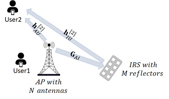
Figure 1: System Model with $K=2$ users.

III IRS-Aided NOMA

In this paper, we consider a scenario where two users with different clusters are being served. In other words, we aim to investigate the effects of inter-cluster interference rather than intra-cluster effect. Clusters here refer to classification of effective channels into superior channels and inferior channels in a NOMA system. Thus, throughout this paper, we assume $K=2$. With these assumptions, the information bearing vector $\mathbf{s}\in\mathbb{C}^{2\times 1}$ is expressed as $\mathbf{s}=\left[\alpha_{1}s^{[1]},\alpha_{2}s^{[2]}\right]^{T}$, where $s^{[i]}$ represents the signal and $\alpha_{i}$ denotes the corresponding power allocation coefficient for the $i$-th user satisfying $\alpha_{1}^{2}+\alpha_{2}^{2}=1$. Let $i$ and $k$ denote the index of two users served by IRS-aided NOMA. In this case, $\mathbf{x}^{[i]}\triangleq\mathbf{w}_{i}s^{[i]}$ denotes the transmit vector intended for the $i$-th user, where $\mathbf{w}_{i}$ is the $i$th active beamforming vector at the AP. The signal received by the $i$-th user is then written by

$$y^{[i]} =\left(\mathbf{h}_{AU}^{[i]}+\mathbf{h}_{IU}^{[i]}\mathbf{\Psi}\mathbf{G}_{AI}\right)\alpha_{i}\mathbf{x}^{[i]}+\left(\mathbf{h}_{AU}^{[i]}+\mathbf{h}_{IU}^{[i]}\mathbf{\Psi}\mathbf{G}_{AI}\right)\alpha_{k}\mathbf{x}^{[k]}+n^{[i]}$$

$$=\alpha_{i}\mathbf{h}^{[i]}\mathbf{x}^{[i]}+\alpha_{k}\mathbf{h}^{[i]}\mathbf{x}^{[k]}+n^{[i]}$$ (3)

where $\mathbf{\Psi}$ represents the diagonal phase shift matrix of the IRS, the effective AP-user channel vector $\mathbf{h}^{[i]}$ is defined by $\mathbf{h}^{[i]}=\mathbf{h}_{AU}^{[i]}+\mathbf{h}_{IU}^{[i]}\mathbf{\Psi}\mathbf{G}_{AI}$ and $n^{[i]}$ is the additive white Gaussian noise with variance $\sigma_{n}^{2}$. Now, by reformulating the received signal in (III) in terms of the estimated channels, we have

$$y^{[i]} =\left(\hat{\mathbf{h}}_{AU}^{[i]}+\hat{\mathbf{h}}_{IU}^{[i]}\mathbf{\Psi}\mathbf{G}_{AI}\right)\alpha_{i}\mathbf{x}^{[i]}+\left(\hat{\mathbf{h}}_{AU}^{[i]}+\hat{\mathbf{h}}_{IU}^{[i]}\mathbf{\Psi}\mathbf{G}_{AI}\right)\alpha_{k}\mathbf{x}^{[k]}$$

$$\quad+\sum_{j=1}^{2}\left[\left(\tilde{\mathbf{h}}_{AU}^{[i]}+\tilde{\mathbf{h}}_{IU}^{[i]}\mathbf{\Psi}\mathbf{G}_{AI}\right)\alpha_{j}\mathbf{x}^{[j]}\right]+n^{[i]}$$

$$=\alpha_{i}\hat{\mathbf{h}}^{[i]}\mathbf{x}^{[i]}+\alpha_{k}\hat{\mathbf{h}}^{[i]}\mathbf{x}^{[k]}+\sum_{j=1}^{2}\left[\alpha_{j}\tilde{\mathbf{h}}^{[i]}\mathbf{x}^{[j]}\right]+n^{[i]},$$ (4)

where

$$\hat{\mathbf{h}}^{[i]}\triangleq\hat{\mathbf{h}}_{AU}^{[i]}+\mathbf{v}\hat{\mathbf{H}}^{[i]}_{c},$$ (5)

$$\tilde{\mathbf{h}}^{[i]}\triangleq\tilde{\mathbf{h}}_{AU}^{[i]}+\mathbf{v}\tilde{\mathbf{H}}^{[i]}_{c},$$ (6)

$$\mathbf{v}\triangleq\left(\operatorname{diag}\left(\mathbf{\Psi}\right)\right)^{T}=\left[\theta_{1},\dots,\theta_{M}\right].$$ (7)

In (5) and (6), $\hat{\mathbf{H}}^{[i]}_{c}=\operatorname{diag}\left(\hat{\mathbf{h}}_{IU}^{[i]}\right)\mathbf{G}_{AI}$ is the estimated cascaded AP-IRS-user channel and $\tilde{\mathbf{H}}^{[i]}_{c}=\operatorname{diag}\left(\tilde{\mathbf{h}}_{IU}^{[i]}\right)\mathbf{G}_{AI}$ represents the cascaded channel estimation error. The distribution of the effective channel estimation error vector $\tilde{\mathbf{h}}^{[i]}$ for large values of $M$ is approximated by

$$\tilde{\mathbf{h}}^{[i]}\sim\mathcal{CN}\left(0,\sigma_{h}^{2}\mathbf{I}\right),$$ (8)

where $\sigma_{h}^{2}=\sigma_{AU}^{2}+M\sigma_{IU}^{2}\beta_{AI}$. The approximation in (8) is derived in the appendix of [10] where it is shown that this approximation becomes more accurate when number of IRS elements is large. Also, it can be easily shown that this approximation remains valid whether the IRS phase shifts are continuous or discrete. Without loss of generality, we assume that the effective channel conditions of the first user is better than the second one [34], i.e. $|\hat{\mathbf{h}}^{[1]}\mathbf{w}_{1}|^{2}\geq|\hat{\mathbf{h}}^{[2]}\mathbf{w}_{2}|^{2}$. With this assumption, the following theorem can be presented.

Theorem 1.

The achievable sum rate of the users is obtained by

$$R^{[sum]}=R^{[1]}+R^{[2]},$$ (9)

in which

$$R^{[1]}=\log_{2}\left(1+\frac{\alpha_{1}^{2}|\hat{\mathbf{h}}^{[1]}\mathbf{w}_{1}|^{2}}{\sigma_{h}^{2}\left(||\mathbf{w}_{1}||^{2}+||\mathbf{w}_{2}||^{2}\right)+\sigma_{n}^{2}}\right),$$ (10)

is the minimum achievable rate of the first user and

$$R^{[2]}=\log_{2}\left(1+\frac{\alpha_{2}^{2}|\hat{\mathbf{h}}^{[2]}\mathbf{w}_{2}|^{2}}{\alpha_{1}^{2}|\hat{\mathbf{h}}^{[2]}\mathbf{w}_{1}|^{2}+\sigma_{h}^{2}\left(||\mathbf{w}_{1}||^{2}+||\mathbf{w}_{2}||^{2}\right)+\sigma_{n}^{2}}\right),$$ (11)

is the minimum achievable rate of the second user.

The proof of Theorem 1 is given in Appendix A.

In this paper, we aim to jointly optimize the active beamforming at the AP and the phase shifts at the IRS to maximize the sum achievable data rate. Specifically, the optimization problem is formulated as follows

$$\begin{array}[]{cl}\max\limits_{\mathbf{w}_{1},\mathbf{w}_{2},\mathbf{v},\alpha_{1},\alpha_{2}}&R^{[sum]}\\ \operatorname{s.t.}&|\theta_{i}|=1,i=1,...,M,\\ &\operatorname{trace}\left(\mathbf{W}\mathbf{W}^{H}\right)\leq P,\\ &\alpha_{1}^{2}+\alpha_{2}^{2}=1,\\ &\left|\hat{\mathbf{h}}^{[1]}\mathbf{w}_{1}\right|^{2}\geq\left|\hat{\mathbf{h}}^{[2]}\mathbf{w}_{2}\right|^{2}.\end{array}$$ (12)

where $\mathbf{W}=[\mathbf{w}_{1},\mathbf{w}_{2}]$. It can be easily observed that this optimization problem is non-convex, with coupled variables. Specifically, the optimization problem (12) incorporates $R^{[1]}$ and $R^{[2]}$ which are nonlinear components with respect to $\mathbf{v}$, $\mathbf{W}_{i}$ and $\alpha_{i}$, and make the problem non-convex. Additionally, the forth constraint in (12) implies a strong and mutual coupling between $\mathbf{v}$ and $\mathbf{w}_{i}$ which can be hardly dealt with in its initial construction. To address these issues, in the following a low-complexity algorithm is presented for addressing this problem.

III-A PDD-based Solution: Continuous Phase shifters

In this section, we propose the PDD-based algorithm [26, 35] to solve the problem in (12). To this end, we first introduce a set of auxiliary variables as $\mathcal{S}=\{\mathbf{T},\mathbf{v},\mathbf{W},\mathbf{a},\bar{\mathbf{W}},\bar{\mathbf{T}},\bar{\mathbf{a}}\}$, where $\mathbf{T}=\mathbf{W}^{H}\hat{\mathbf{H}}^{H}$, $\hat{\mathbf{H}}\triangleq\left[\hat{\mathbf{h}}^{[1]\ T},\hat{\mathbf{h}}^{[2]\ T}\right]^{T}$, $\mathbf{a}=[\alpha_{1},\alpha_{2}]^{T}$, $\bar{\mathbf{W}}=\mathbf{W}$, $\bar{\mathbf{T}}=\mathbf{T}$, and $\bar{\mathbf{a}}=\mathbf{a}$. With these definitions, the optimization problem becomes

$$\begin{array}[]{cl}\max\limits_{\mathcal{S}}&\log_{2}\left(1+\frac{\alpha_{1}^{2}|t_{11}|^{2}}{\sigma_{h}^{2}\left(||\mathbf{w}_{1}||^{2}+||\mathbf{w}_{2}||^{2}\right)+\sigma_{n}^{2}}\right)+\log_{2}\left(1+\frac{\alpha_{2}^{2}|t_{22}|^{2}}{\alpha_{1}^{2}|t_{12}|^{2}+\sigma_{h}^{2}\left(||\mathbf{w}_{1}||^{2}+||\mathbf{w}_{2}||^{2}\right)+\sigma_{n}^{2}}\right)\\ \operatorname{s.t.}&|\theta_{i}|=1,i=1,...,M,\\ &\operatorname{trace}\left(\bar{\mathbf{W}}\bar{\mathbf{W}}^{H}\right)\leq P,\\ &\bar{\mathbf{a}}^{T}\bar{\mathbf{a}}=1,\\ &\left|\bar{t}_{11}\right|^{2}\geq\left|\bar{t}_{22}\right|^{2},\\ &\mathbf{T}=\mathbf{W}^{H}\hat{\mathbf{h}}^{H},\bar{\mathbf{T}}=\mathbf{T},\bar{\mathbf{W}}=\mathbf{W},\bar{\mathbf{a}}=\mathbf{a}.\end{array}$$ (13)

Furthermore, to obtain the augmented Lagrangian problem, the equality conditions should be put into the objective function. This leads to the following optimization problem

$$\begin{array}[]{cl}\max\limits_{\mathcal{S}}&\log_{2}\left(1+\frac{\alpha_{1}^{2}|t_{11}|^{2}}{\sigma_{h}^{2}\left(||\mathbf{w}_{1}||^{2}+||\mathbf{w}_{2}||^{2}\right)+\sigma_{n}^{2}}\right)+\log_{2}\left(1+\frac{\alpha_{2}^{2}|t_{22}|^{2}}{\alpha_{1}^{2}|t_{12}|^{2}+\sigma_{h}^{2}\left(||\mathbf{w}_{1}||^{2}+||\mathbf{w}_{2}||^{2}\right)+\sigma_{n}^{2}}\right)-Q_{\gamma}(\mathcal{S})\\ \operatorname{s.t.}&|\theta_{i}|=1,i=1,...,M,\\ &\operatorname{trace}\left(\bar{\mathbf{W}}\bar{\mathbf{W}}^{H}\right)\leq P,\\ &\bar{\mathbf{a}}^{T}\bar{\mathbf{a}}=1,\\ &\left|\bar{t}_{11}\right|^{2}\geq\left|\bar{t}_{22}\right|^{2},\\ \end{array}$$ (14)

where $Q_{\gamma}(\mathcal{S})$ is calculated by

$$\small Q_{\gamma}(\mathcal{S})=\frac{1}{2\gamma}\Big{(} \sum_{i=1}^{2}||\mathbf{w}_{i}-\bar{\mathbf{W}}_{i}+\gamma\boldsymbol{\lambda}_{w_{i}}||^{2}+\sum_{i=1}^{2}\sum_{j=1}^{2}|t_{ij}-\mathbf{w}_{i}^{H}\hat{\mathbf{h}}^{[j]H}+\gamma{\lambda}_{{h}_{ij}}|^{2}$$

$$+\sum_{i=1}^{2}\sum_{j=1}^{2}|{t}_{ij}-\bar{{t}}_{ij}+\gamma{\lambda}_{t_{ij}}|^{2}+\sum_{i=1}^{2}|\alpha_{i}-\bar{\alpha}_{i}+\gamma{\lambda}_{a_{i}}|^{2}\Big{)}.$$ (15)

The penalty parameter for the Lagrangian function is denoted by $\gamma$, and $\boldsymbol{\lambda}_{w_{i}}$, $\lambda_{h_{ij}}$, $\lambda_{t_{ij}}$ and $\lambda_{a_{i}}$, $i,j\in\{1,2\}$, are the dual variables of the equality conditions in problem (13). The vector $\boldsymbol{\lambda}_{w_{i}}$ is the $i$th column of the matrix $\boldsymbol{\Lambda}_{w}$ and $\lambda_{h_{ij}}$, $\lambda_{t_{ij}}$ and $\lambda_{a_{i}}$ are the elements of $\boldsymbol{\Lambda}_{h}$, $\boldsymbol{\Lambda}_{t}$ and $\boldsymbol{\lambda}_{a}$, respectively. Note that, here one of the equality conditions is not put into the objective function. The reason is that by keeping this condition in the constrains, a closed-form solution can be calculated with projection. The details are explained later in this paper.

Now to apply BSUM to (14), we introduce the following theorem.

Theorem 2.

The objective function of the optimization problem in (13) can be rewritten as

$$\max\limits_{q_{1},q_{2},d_{1},d_{2}}\sum_{i=1}^{2}\Big{(}\log(d_{i})-d_{i}f_{i}(q_{i},\mathcal{S})\Big{)}+2,$$ (16)

where

$$f_{1}(q_{1},\mathcal{S}) =|1-q_{1}^{*}\alpha_{1}t_{11}|^{2}+\sigma_{h}^{2}(||q_{1}^{*}\mathbf{w}_{1}||^{2}+||q_{1}^{*}\mathbf{w}_{2}||^{2})+\sigma_{n}^{2}|q_{1}|^{2},$$ (17)

$$f_{2}(q_{2},\mathcal{S}) =|1-q_{2}^{*}\alpha_{2}t_{22}|^{2}+\alpha_{1}^{2}|q_{2}^{*}t_{12}|^{2}+\sigma_{h}^{2}(||q_{2}^{*}\mathbf{w}_{1}||^{2}+||q_{2}^{*}\mathbf{w}_{2}||^{2})+\sigma_{n}^{2}|q_{2}|^{2}.$$ (18)

The proof of this theorem can be simply finished by using the first order equality condition on the equation (16), to obtain the optimal values for $q_{1}$, $q_{2}$, $d_{1}$ and $d_{2}$ as

$$q_{1}^{opt}(\mathcal{S})=\frac{\alpha_{1}t_{11}}{\alpha_{1}^{2}|t_{11}|^{2}+\sigma_{h}^{2}\left(||\mathbf{w}_{1}||^{2}+||\mathbf{w}_{2}||^{2}\right)+\sigma_{n}^{2}},$$ (19)

$$q_{2}^{opt}(\mathcal{S})=\frac{\alpha_{2}t_{22}}{\alpha_{2}^{2}|t_{22}|^{2}+\alpha_{1}^{2}|t_{12}|^{2}+\sigma_{h}^{2}\left(||\mathbf{w}_{1}||^{2}+||\mathbf{w}_{2}||^{2}\right)+\sigma_{n}^{2}},$$ (20)

$$d_{1}^{opt}(\mathcal{S})=1+\frac{\alpha_{1}^{2}|t_{11}|^{2}}{\sigma_{h}^{2}\left(||\mathbf{w}_{1}||^{2}+||\mathbf{w}_{2}||^{2}\right)+\sigma_{n}^{2}},$$ (21)

$$d_{2}^{opt}(\mathcal{S})=1+\frac{\alpha_{2}^{2}|t_{22}|^{2}}{\alpha_{1}^{2}|t_{12}|^{2}+\sigma_{h}^{2}\left(||\mathbf{w}_{1}||^{2}+||\mathbf{w}_{2}||^{2}\right)+\sigma_{n}^{2}}.$$ (22)

This theorem gives a lower bound for the objective function of (13) as

$$\log_{2}\left(1+\frac{\alpha_{1}^{2}|t_{11}|^{2}}{\sigma_{h}^{2}\left(||\mathbf{w}_{1}||^{2}+||\mathbf{w}_{2}||^{2}\right)+\sigma_{n}^{2}}\right)+\log_{2}\left(1+\frac{\alpha_{2}^{2}|t_{22}|^{2}}{\alpha_{1}^{2}|t_{12}|^{2}+\sigma_{h}^{2}\left(||\mathbf{w}_{1}||^{2}+||\mathbf{w}_{2}||^{2}\right)+\sigma_{n}^{2}}\right)$$

$$\geq\sum_{i=1}^{2}\Big{(}\log(d_{i}^{opt}(\mathcal{S}))-d_{i}^{opt}(\mathcal{S})f_{i}(q_{i}^{opt}(\mathcal{S}),\mathcal{S})\Big{)}+2.$$ (23)

This locally tight lower bound is tractable and by using it instead of its original equation, the BSUM can be applied to our problem. Then, the new form of the optimization problem becomes

$$\begin{array}[]{cl}\min\limits_{\mathcal{S}}&\sum_{i=1}^{2}d_{i}(\mathcal{S})f_{i}(q_{i}(\mathcal{S}),\mathcal{S})+Q_{\gamma}(\mathcal{S})\\ \operatorname{s.t.}&|\theta_{i}|=1,i=1,...,M,\\ &\operatorname{trace}\left(\bar{\mathbf{W}}\bar{\mathbf{W}}^{H}\right)\leq P,\\ &\bar{\mathbf{a}}^{T}\bar{\mathbf{a}}=1,\\ &\left|\bar{t}_{11}\right|^{2}\geq\left|\bar{t}_{22}\right|^{2}.\\ \end{array}$$ (24)

Now, by applying the BSUM, the optimization problem in (24) can be solved via the following steps, each resulting in a closed-form solution for a sub-set of the variables.

At first, we solve the problem based on $\mathbf{W}$ while considering all other variables as constants. Based on the first order optimality condition we can obtain the solution as

$$\mathbf{w}_{1}= \left(2\gamma|q_{1}|^{2}d_{1}\sigma_{h}^{2}\mathbf{I}+2\gamma|q_{2}|^{2}d_{2}\sigma_{h}^{2}\mathbf{I}+\mathbf{I}+\sum_{j=1}^{2}\hat{\mathbf{h}}^{[j]H}\hat{\mathbf{h}}^{[j]}\right)^{-1}$$

$$\times\left(\bar{\mathbf{W}}_{1}-\gamma\boldsymbol{\lambda}_{w_{1}}+\sum_{j=1}^{2}(\hat{\mathbf{h}}^{[j]H}t_{1j}^{*}+\hat{\mathbf{h}}^{[j]H}\gamma\lambda_{h_{1j}}^{*})\right),$$ (25)

$$\mathbf{w}_{2} =\left(2\gamma|q_{1}|^{2}d_{1}\sigma_{h}^{2}\mathbf{I}+2\gamma|q_{2}|^{2}d_{2}\sigma_{h}^{2}\mathbf{I}+\mathbf{I}+\sum_{j=1}^{2}\hat{\mathbf{h}}^{[j]H}\hat{\mathbf{h}}^{[j]}\right)^{-1}$$

$$\times\left(\bar{\mathbf{W}}_{2}-\gamma\boldsymbol{\lambda}_{w_{2}}+\sum_{j=1}^{2}(\hat{\mathbf{h}}^{[j]H}t_{2j}^{*}+\hat{\mathbf{h}}^{[j]H}\gamma\lambda_{h_{2j}}^{*})\right).$$ (26)

Secondly, we find the optimal values for $\alpha_{1}$ and $\alpha_{2}$ based on the first order optimality condition, as

$$\alpha_{1}=\frac{2\gamma d_{1}\operatorname{Re}\{q_{1}t_{11}^{*}\}+\bar{\alpha}_{1}-\gamma\lambda_{a_{1}}}{1+2\gamma d_{1}|q_{1}|^{2}|t_{11}|^{2}+2\gamma d_{2}|q_{2}^{*}t_{12}|^{2}},$$ (27)

$$\alpha_{2}=\frac{2\gamma d_{2}\operatorname{Re}\{q_{2}^{*}t_{22}\}+\bar{\alpha}_{2}-\gamma\lambda_{a_{2}}}{1+2\gamma d_{2}|q_{2}|^{2}|t_{22}|^{2}}.$$ (28)

In the next step, we use the same method for the variable $\mathbf{T}$. The closed-form solution for each element of this variable is

$$t_{11}=\frac{2\gamma d_{1}q_{1}\alpha_{1}+\mathbf{w}_{1}^{H}\hat{\mathbf{h}}^{[1]H}+\bar{t}_{11}-\gamma(\lambda_{h_{11}}+\lambda_{t_{11}})}{2\gamma d_{1}|q_{1}|^{2}\alpha_{1}^{2}+2},$$ (29)

$$t_{12}=\frac{\mathbf{w}_{1}^{H}\hat{\mathbf{h}}^{[2]H}+\bar{t}_{12}-\gamma(\lambda_{h_{12}}+\lambda_{t_{12}})}{2\gamma d_{2}\alpha_{1}^{2}|q_{2}|^{2}+2},$$ (30)

$$t_{21}=\frac{1}{2}\left(\mathbf{w}_{2}^{H}\hat{\mathbf{h}}^{[1]H}+\bar{t}_{21}-\gamma(\lambda_{h_{21}}+\lambda_{t_{21}})\right),$$ (31)

$$t_{22}=\frac{2\gamma d_{2}q_{2}\alpha_{2}+\mathbf{w}_{2}^{H}\hat{\mathbf{h}}^{[2]H}+\bar{t}_{22}-\gamma(\lambda_{h_{22}}+\lambda_{t_{22}})}{2\gamma d_{2}|q_{2}|^{2}\alpha_{2}^{2}+2}.$$ (32)

Then, the optimization problem with respect to $\bar{\mathbf{T}}$ is solved, as

$$\bar{\mathbf{T}}=\begin{cases}\mathbf{Y},&|y_{11}|^{2}\geq|y_{22}|^{2}\\ \begin{bmatrix}\frac{y_{11}-y_{22}}{2}&y_{12}\\ y_{21}&\frac{y_{11}-y_{22}}{2}\end{bmatrix}\text{or}\begin{bmatrix}\frac{y_{11}+y_{22}}{2}&y_{12}\\ y_{21}&\frac{y_{11}+y_{22}}{2}\end{bmatrix},&|y_{11}|^{2}<|y_{22}|^{2}\end{cases}.$$ (33)

In (33), $\mathbf{Y}=\mathbf{T}+\gamma\boldsymbol{\Lambda}_{x}$ and $y_{ij}$ represents the element in the $i$th row and the $j$th column of matrix $\mathbf{Y}$. Also, in case $|y_{11}|^{2}<|y_{22}|^{2}$, the matrix with the least Euclidean distance to $\mathbf{Y}$ would be selected as $\bar{\mathbf{T}}$.

Next, we need to consider the auxiliary variables $\bar{\mathbf{W}}$ and $\bar{\mathbf{a}}$. The corresponding constraint for $\bar{\mathbf{W}}$ is a projection of a point onto a ball centered at the origin. The closed-form solution for this exists as

$$\bar{\mathbf{W}}=\mathcal{P}_{P}(\mathbf{W}+\gamma\boldsymbol{\Lambda}_{w}).$$ (34)

Similarly, the corresponding constraint for $\bar{\mathbf{a}}$ can be satisfied by projection of a point onto a circle and the closed-form solutions for $\bar{\alpha}_{1}$ and $\bar{\alpha}_{2}$ are calculated as

$$\bar{\alpha}_{1}=\sqrt{\frac{1}{1+(\frac{\alpha_{2}+\gamma\lambda_{a_{2}}}{\alpha_{1}+\gamma\lambda_{a_{1}}})^{2}}},$$ (35)

$$\bar{\alpha}_{2}=(\frac{\alpha_{2}+\gamma\lambda_{a_{2}}}{\alpha_{1}+\gamma\lambda_{a_{1}}})\bar{\alpha}_{1}.$$ (36)

The final step is to solve the problem for the variable $\mathbf{v}$. In this case, the problem could be rewritten as

$$\begin{array}[]{cl}\min\limits_{|\theta_{i}|=1,i=1,...,M}&\mathbf{v}\mathbf{A}\mathbf{v}^{H}-2\operatorname{Re}\{\mathbf{c}\mathbf{v}^{H}\},\end{array}$$ (37)

where,

$$\mathbf{A}=\frac{1}{2\gamma}\sum_{i=1}^{K}\sum_{j=1}^{K}\hat{\mathbf{H}}^{[j]}_{c}\mathbf{w}_{i}\mathbf{w}_{i}^{H}\hat{\mathbf{H}}^{[j]H}_{c},$$ (38)

$$\small\mathbf{c}=\frac{1}{2\gamma}\sum_{i=1}^{K}\sum_{j=1}^{K}\left(t_{ij}^{*}+\gamma\lambda_{h_{ij}}^{*}-\hat{\mathbf{h}}_{AU}^{[j]}\mathbf{w}_{i}\right)\mathbf{w}_{i}^{H}\hat{\mathbf{H}}^{[j]H}_{c}.$$ (39)

Now for one specified $\theta_{k},k=1,...,M$, the optimization problem becomes

$$\begin{array}[]{cl}\min\limits_{|\theta_{k}|=1}&|\theta_{k}|^{2}{a}_{kk}-2\operatorname{Re}\{({c}_{k}-\sum_{i\neq k}^{M}\theta_{i}{a}_{ik})\theta_{k}^{*}\},\end{array}$$ (40)

and the solution to this optimization problem is

$$\theta_{k}=\frac{{c}_{k}-\sum_{i\neq k}^{M}\theta_{i}{a}_{ik}}{|{c}_{k}-\sum_{i\neq k}^{M}\theta_{i}{a}_{ik}|}.$$ (41)

Then, an iterative algorithm is proposed to alternately optimize one phase shift while keeping the others fixed until final convergence.

The steps of the PDD algorithm using BSUM to solve the optimization problem in (24) are described in Algorithm 1. The steps of the basic PDD method in which the dual variables and the penalty parameter are updated, in addition to a detailed convergence analysis for this scheme are provided in [26]. Specifically, it is shown that under appropriate conditions, the sequence of $\mathbf{t}^{k}\in\mathcal{S}$ generated by the PDD method tends to a KKT point of the main problem. In Algorithm 1, the update method for the dual variable $\boldsymbol{\lambda}_{a}$ in the $k$th iteration is as follows

$$\boldsymbol{\lambda}_{a}^{k}=\boldsymbol{\lambda}_{a}^{k-1}+\frac{1}{\gamma}(\mathbf{a}-\bar{\mathbf{a}}).$$ (42)

The other dual Lagrangian variables, e.g. $\boldsymbol{\Lambda}_{h},\boldsymbol{\Lambda}_{w},\boldsymbol{\Lambda}_{t}$ are updated in the same manner. Also, the penalty parameter in the $k$th iteration is updated by

$$\gamma^{k}=\zeta\gamma^{k-1},$$ (43)

where $\zeta\in(0,1)$ is a decreasing parameter.

Algorithm 1 The PDD algorithm using BSUM to solve the problem in (24)

  $\mathbf{Initialize}$  $\gamma,\boldsymbol{\Lambda}_{h},\boldsymbol{\Lambda}_{w},\boldsymbol{\Lambda}_{t},\boldsymbol{\lambda}_{a},\epsilon,\eta,\zeta$

  $\mathbf{Initialize}$  $\mathbf{v},\mathbf{W}$ and $\mathbf{a}$ such that all constraints are met

  $\mathbf{Compute}$ $\hat{\mathbf{h}}$ based on (5)

  $\mathbf{Set}$    $\mathbf{T}=\mathbf{W}^{H}\hat{\mathbf{h}}^{H},\bar{\mathbf{W}}=\mathbf{W}$, $\bar{\mathbf{T}}=\mathbf{T}$, $\bar{\mathbf{a}}=\mathbf{a}$

  $\mathbf{Repeat}$

   1. Compute $q_{i}^{opt}$ and $d_{i}^{opt}$ by (19)-(22)

   2. Compute $\mathbf{W}$ by (III-A), (III-A)

   3. Compute $\mathbf{a}$ by (27), (28)

   4. Compute $\mathbf{T}$ by (29)-(32)

   5. Compute $\bar{\mathbf{T}}$ by (33)

   6. Compute $\bar{\mathbf{W}}$, $\bar{\mathbf{a}}$ by (34), (35), (36)

   7. Compute $\mathbf{v}$ by solving (37) in an iterative algorithm

   8. Recalculate $\mathbf{\hat{G}}$ with the updated $\mathbf{v}$ by (5)

   9. Calculate the Frobenius norms of $||\mathbf{T}-\mathbf{W}^{H}\hat{\mathbf{h}}^{H}||$,  $||\mathbf{W}-\bar{\mathbf{W}}||$, $||\mathbf{T}-\bar{\mathbf{T}}||$ and $||\mathbf{a}-\bar{\mathbf{a}}||$.

   10. If the value of calculated  norms $\leq\eta$

     Update $\boldsymbol{\Lambda}_{h},\boldsymbol{\Lambda}_{w},\boldsymbol{\Lambda}_{t},\boldsymbol{\lambda}_{a}$ as in (42)

    else

     Update $\gamma$ by (43)

    end if

  $\mathbf{Until}$ the absolute difference of two consecutive sum-rates is less than $\epsilon$.

III-B PDD-based Solution: Discrete Phase Shifters

In case of discrete phase shifters for the IRS, the phase of each IRS element should be optimally chosen from a set of $M_{IRS}$ discrete phase shifts. In this case, to solve the problem in (24), we employ the PDD algorithm as in the previous sub-section. All of the steps of the algorithm are the same as the continuous IRS case, except for the seventh step in which the variable $\mathbf{v}$ is calculated. In this case, the problem in (37) can be rewritten as

$$\begin{array}[]{cl}\min\limits_{\theta_{k}\in\mathbf{\Psi}_{N},k=1,...,M}&R_{trellis},\end{array}$$ (44)

where

$$R_{trellis}=\sum_{j=1}^{M}\operatorname{Re}\left\{(\sum_{i=1}^{j-1}\theta_{j}^{*}a_{ij}\theta_{i})-c_{j}\theta_{j}^{*}\right\}.$$ (45)

Note that the objective function in (44) is in the form of a consecutive real summation; therefore we can use the trellis algorithm to find the best discrete IRS phase shifts [36].

For the sake of solving Problem (44), let $T$ be the number of variables ($\theta_{i}$) as the memory, each having $M_{IRS}$ possible choices. Therefore, as depicted in Fig. 2, we construct a trellis with $(M_{IRS})^{T}$ states, each having $M_{IRS}$ outgoing branches with labels selected from $\mathbf{\Psi}_{N}$.

We describe the details of the proposed algorithm as follows. At first, the initial $T$ variables are taken as initial memory values and their $(M_{IRS})^{T}$ possible permutations form the trellis states. Initial benchmarks are calculated by inserting the values of each state in the first $T$ terms of the objective function of (44). At the $n$-th stage, the branch labels imply the $(n+T)$-th variable ($\theta_{n+T}$), and the branch benchmark is the ($n+T$)-th term of the objective function of (44). At each stage, the cumulative benchmark of branches are calculated by adding the branch benchmarks to the cumulative benchmark of their originating paths. After that, among the branches entering the same state, the branch with the least cumulative benchmark is kept and the others are removed. The algorithm is terminated after $M-T$ stages and the path with the minimum cumulative benchmark is selected as the final solution. The labels on the selected path represent the latter $M-T$ variables, and the initial state associated with the selected path stands for the first $T$ variables. This process is shown in Algorithm 2. The overall solution is the same as Algorithm 1, but instead of its 7th step, we employ the method in Algorithm 2. For more details on the trellis algorithm please refer to [37].

Algorithm 2 Trellis-based discrete phase shift determination for the IRS

  $\mathbf{Input}:$ $\mathbf{\Psi}_{N},\mathbf{v}^{Initial}$

  $\mathbf{Output}:$ $\mathbf{v}$

  $\mathbf{Initialize}$ all possible permutations of $\theta_{1},\dots,\theta_{T}$

  for $i=T+1,\dots,M$ do

     for $j=1,\dots,M_{IRS}$ do

        $\theta_{i}=\mathbf{\Psi}_{N}(j)$;

        calculate (45) as the benchmark;

     end for

     eliminate all paths except the one with the minimum benchmark value;

  end for

  Choose $\theta_{i},\dots,\theta_{M}$, such that they lead to the minimum cumulative benchmark value.

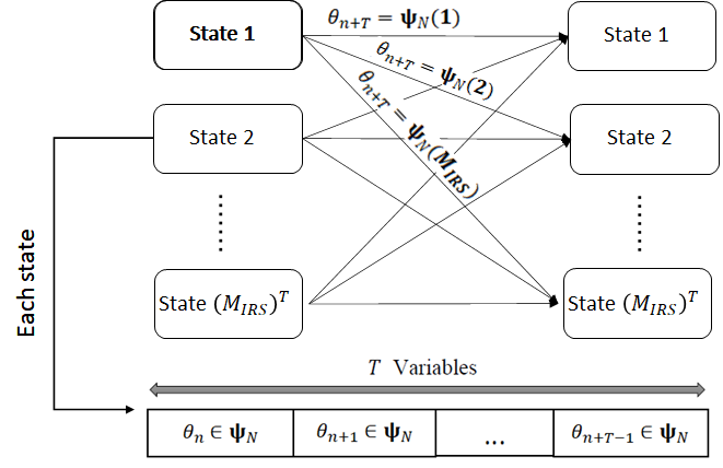
Figure 2: Trellis-based design for determination of $\mathbf{v}$.

IV Complexity Analysis

In this section, the complexity of the proposed method is calculated for both cases of continuous and discrete IRS, and it is compared with other techniques in the literature.

IV-A Continuous IRS

The proposed scheme in Algorithm 1 is iterative. In each iteration, the computational complexity consists of calculating the variables in steps $1$ through $10$ of Algorithm 1 and updating either the dual Lagrangian variables or the penalty parameter. Note that in step $10$, the order of complexity is highest when the dual variables are being updated. Also, for step 7 of the continuous IRS case, the order of computational complexity is approximated by the computational complexity of equations (38) and (39) since it relies on $M$ which is large. Considering a $K=2$ user system, the order of complexity of each step in Algorithm 1, for a continuous IRS, is

$$\mathcal{O}(6M^{2}+(2N^{2}+8N)M+2N^{3}+21N^{2}+157N).$$ (46)

This order of complexity is lower than that of the methods in the literature focusing on sum-rate maximization in the downlink. In [16], an alternating optimization technique in used to find optimal active AP beamforming vector and the passive IRS phase shifts for the sum-rate maximization problem. The authors used the interior-point solver in CVX to solve the resulting convex optimization problems in each iteration of their algorithm which scales up the order of complexity. For instance the complexity of each iteration of the algorithm proposed in [16] is

$$\mathcal{O}(\max(N,3K(K-1)^{4})\sqrt{N}\log(\frac{1}{\mu_{c}})+(3K^{2}+M)^{3.5}),$$ (47)

where $\mu_{c}$ is the accuracy defined in [16]. Specifically speaking, consider a simple case where $N=K=2$ and $M=50$, which are low dimensions for the system model, and assume that $\mu_{c}=0.1$. In this scenario, the order of complexity of the algorithm proposed in [16] is 100 times the complexity of our proposed scheme. Fig. 3 better demonstrates the complexity ratio of the algorithm in [16] to our PDD-based proposed method in different system dimensions. As shown in this figure and based on the equations (46) and (47), the complexity of our method rises with $N^{3}$ while the complexity of the other algorithm rises with $N$, but still even for large values of $N$, the complexity of our method is far less.

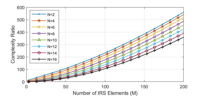
Figure 3: Complexity ratio each iteration of the algorithm in [16] to each iteration of our PDD-based proposed algorithm.

IV-B Discrete IRS

In case of the discrete IRS, the 7th step of the Algorithm 1 is replaced with Algorithm 2. The proposed trellis-based algorithms consist of $M-T$ stages. The optimization of $\mathbf{v}$ consists of $(M_{IRS})^{T}$ states with $M_{IRS}$ branches entering each state. Hence, a total of $(M-T)(M_{IRS})^{T+1}$ comparisons are needed. This number is negligible compared with an exhaustive search method with $(M_{IRS})^{M}$ comparisons, especially for large values of $M$. By using the trellis-based algorithm, the computational complexity of each step of Algorithm 1 becomes

$$\mathcal{O}(2M^{2}+4NM+2N^{3}+20N^{2}+150N+(M-T)(M_{IRS})^{T+1}).$$ (48)

In case of using exhaustive search instead of trellis, the last term on (48) is replaced by $(M_{IRS})^{M}$, while if we use the quantization technique the last term of (48) is replaced by $M$. To better understand, consider a system model with the following variables $K=2$, $M=20$, $N=2$, $T=3$ and $M_{IRS}=4$. In this case the order of complexity for the trellis based method is $4.1$ times that of the quantization method and $5\times 10^{-9}$ times that of the exhaustive search algorithm.

V IRS-Aided OMA

In this section we consider IRS-aided FDMA and TDMA communication systems to provide a comparison benchmark for IRS-aided NOMA. Here, as in the IRS-NOMA scenario, it is assumed that the acquired CSI is with an estimation error with the power of $\sigma_{h}^{2}$. In the following, the FDMA and TDMA cases are considered and a robust solution is given that maximizes their sum-rates.

V-A FDMA Mode

In the FDMA mode, the AP communicates with the two users over two adjacent frequency resource blocks. In this case, the achievable sum-rate is calculated by

$$R^{[sum]}_{\text{FDMA}}=\frac{1}{2}\sum_{k=1}^{2}\log_{2}\left(1+\frac{|{\hat{\mathbf{h}}}^{[k]}\mathbf{w}_{k}|^{2}}{\frac{1}{2}\sigma_{h}^{2}||\mathbf{w}_{k}||^{2}+\frac{1}{2}\sigma_{n}^{2}}\right).$$ (49)

The proof can be easily driven with a similar approach to that of theorem 1 in [10]. Therefore, the resultant optimization problem of maximizing the sum-rate is written as

$$\begin{array}[]{cl}\max\limits_{\mathbf{W},\mathbf{v}}&R^{[sum]}_{\text{FDMA}}\\ \operatorname{s.t.}&|\theta_{i}|=1,i=1,...,M,\\ &\operatorname{trace}\left(\mathbf{W}\mathbf{W}^{H}\right)\leq P.\end{array}$$ (50)

To solve this optimization problem we employ the alternating optimization (AO) technique, where in each step the problem is solved for each optimization variable separately until some convergence criteria is met. Assuming that the transmit power on the $k$-th sub-channel is defined by $\mathbf{w}_{k}^{H}\mathbf{w}_{k}=P_{k}$, the optimization problem is presented by

$$\begin{array}[]{cl}\max\limits_{\mathbf{v},P_{k},\mathbf{W}}&\sum_{k=1}^{2}\log_{2}\left(1+\frac{|{\hat{\mathbf{h}}}^{[k]}\mathbf{w}_{k}|^{2}}{\frac{1}{2}P_{k}\sigma_{h}^{2}+\frac{1}{2}\sigma_{n}^{2}}\right)\\ \operatorname{s.t.}&|\theta_{i}|=1,i=1,...,M,\\ &\sum_{k=1}^{K}P_{{k}}\leq P\\ &P_{{k}}\geq 0,\ k=1,\dots K,\\ &\mathbf{w}_{k}^{H}\mathbf{w}_{k}=P_{K},\ k=1,\dots K.\end{array}$$ (51)

At first, we solve the optimization problem with respect to only $\mathbf{W}$. To do so, the optimization problem can be solved separately for each $\mathbf{w}_{k}$. Since the logarithm is monotonically increasing with $|{\hat{\mathbf{h}}}^{[k]}\mathbf{w}_{k}|^{2}$, the solution can be driven by solving the following optimization problem

$$\begin{array}[]{cl}\max\limits_{\mathbf{w}_{k}}&|{\hat{\mathbf{h}}}^{[k]}\mathbf{w}_{k}|^{2}\\ \operatorname{s.t.}&\mathbf{w}_{k}^{H}\mathbf{w}_{k}=P_{K},\ k=1,\dots K.\end{array}$$ (52)

The closed-form solution to the optimization problem in (52) is given by

$$\mathbf{w}_{k}=\sqrt{P_{k}}\frac{\hat{\mathbf{h}}^{[k]H}}{||\hat{\mathbf{h}}^{[k]}||}.$$ (53)

We then rewrite the optimization problem in (51) by having (53) as

$$\begin{array}[]{cl}\max\limits_{\mathbf{v},P_{k}}&\sum_{k=1}^{2}\log_{2}\left(1+\frac{P_{k}||{\hat{\mathbf{h}}}^{[k]}||^{2}}{\frac{1}{2}P_{k}\sigma_{h}^{2}+\frac{1}{2}\sigma_{n}^{2}}\right)\\ \operatorname{s.t.}&|\theta_{i}|=1,i=1,...,M,\\ &\sum_{k=1}^{K}P_{{k}}\leq P\\ &P_{{k}}\geq 0,\ k=1,\dots K.\end{array}$$ (54)

Next, we solve the optimization problem in (54) with respect to the optimization variable $\mathbf{v}$. To do so, the variable $P_{k}$ is considered as constant and since the objective function in (54) is monotonically increasing with $\hat{\mathbf{h}}^{[k]}$, the problem is rewritten as

$$\begin{array}[]{cl}\max\limits_{P_{k},\mathbf{v}}&\sum_{k=1}^{K}P_{{k}}||{\hat{\mathbf{h}}}^{[k]}||^{2}\\ \operatorname{s.t.}&|\theta_{i}|=1,i=1,...,M.\\ \end{array}$$ (55)

Then, for each phase shift value $\theta_{i}$, the optimization problem in (55) becomes

$$\begin{array}[]{cl}\max\limits_{|\theta_{i}|=1}&|\theta_{i}|^{2}{a}_{ii}^{[k]}+2\operatorname{Re}\{(\sum_{j\neq i}^{M}\theta_{j}{a}_{ji}+{c}_{i})\theta_{i}^{*}\},\end{array}$$ (56)

where $a_{ij}$ and $c_{i}$, $i,j=1,...,M$, are the elements of $\mathbf{A}=\sum_{k=1}^{K}\hat{\mathbf{H}}_{c}^{[k]}\hat{\mathbf{H}}_{c}^{[k]H}$ and $\mathbf{c}=\sum_{k=1}^{K}\hat{\mathbf{h}}_{AU}^{[k]}\hat{\mathbf{H}}_{c}^{[k]H}$, respectively. Henceforth, the problem is solved alternately. In the $i$th step considering all other phase shift elements to be known, the optimal phase shift value for the $i$th element would be calculated as

$$\theta_{i}=\frac{\sum_{j\neq i}^{M}\theta_{j}{a}_{ji}+{c}_{i}}{|\sum_{j\neq i}^{M}\theta_{j}{a}_{ji}+{c}_{i}|}.$$ (57)

The optimization problem in (54) with respect to the variable $P_{k},k=1,2$ can be rewritten as

$$\begin{array}[]{cl}\max\limits_{P_{1},P^{{}^{\prime}}}&\log_{2}\left(1+\frac{P_{1}||{\hat{\mathbf{h}}}^{[1]}||^{2}}{\frac{1}{2}P_{1}\sigma_{h}^{2}+\frac{1}{2}\sigma_{n}^{2}}\right)+\log_{2}\left(1+\frac{(P^{{}^{\prime}}-P_{1})||{\hat{\mathbf{h}}}^{[2]}||^{2}}{\frac{1}{2}(P^{{}^{\prime}}-P_{1})\sigma_{h}^{2}+\frac{1}{2}\sigma_{n}^{2}}\right)\\ \operatorname{s.t.}&P^{{}^{\prime}}\leq P,\\ &P_{{1}}\geq 0,\end{array}$$ (58)

in which the variable $P_{2}$ is replaced by $P_{2}=P^{{}^{\prime}}-P_{1}$. By calculating the derivative of the objective function in (58) with respect to $P^{{}^{\prime}}$, it can be seen that the derivative is always positive, and thus it is obvious that the objective function of the problem in (58) is monotonically increasing with $P^{{}^{\prime}}$. Now by taking the constraint $P^{{}^{\prime}}\leq P$ into account, we can conclude that the optimal solution for this variable is $P^{{}^{\prime}}=P$. This can be readily proven by driving the derivative of the objective function of (58) with respect to $P^{{}^{\prime}}$. Thus, the problem is further simplified as

$$\begin{array}[]{cl}\max\limits_{P_{1}}&\log_{2}\left(1+\frac{P_{1}||{\hat{\mathbf{h}}}^{[1]}||^{2}}{\frac{1}{2}P_{1}\sigma_{h}^{2}+\frac{1}{2}\sigma_{n}^{2}}\right)+\log_{2}\left(1+\frac{(P-P_{1})||{\hat{\mathbf{h}}}^{[2]}||^{2}}{\frac{1}{2}(P-P_{1})\sigma_{h}^{2}+\frac{1}{2}\sigma_{n}^{2}}\right)\\ \operatorname{s.t.}&0\leq P_{{1}}\leq P.\end{array}$$ (59)

By driving the derivative of the objective function in (59) with respect to $P_{1}$ and based on the first-order optimality condition, it can be seen that only one optimal solution for $P_{1}$ exists, which can be found by

$$P_{1}=\frac{-B+\sqrt{B^{2}-4AC}}{2A},$$ (60)

where

$$A=\frac{1}{4}\sigma_{h}^{4}(||\hat{\mathbf{h}}^{[1]}||^{2}+||\hat{\mathbf{h}}^{[2]}||^{2}),$$ (61)

$$B= \frac{1}{2}||\hat{\mathbf{h}}^{[2]}||^{2}\sigma_{h}^{2}\sigma_{n}^{2}+\sigma_{n}^{2}||\hat{\mathbf{h}}^{[1]}||^{2}||\hat{\mathbf{h}}^{[2]}||^{2}+\frac{P}{2}\sigma_{h}^{4}||\hat{\mathbf{h}}^{[1]}||^{2}$$

$$+P\sigma_{h}^{2}||\hat{\mathbf{h}}^{[1]}||^{2}||\hat{\mathbf{h}}^{[2]}||^{2}+\frac{1}{2}||\hat{\mathbf{h}}^{[1]}||^{2}\sigma_{h}^{2}\sigma_{n}^{2},$$ (62)

$$C= \frac{1}{4}\sigma_{n}^{4}||\hat{\mathbf{h}}^{[2]}||^{2}-\frac{1}{4}\sigma_{n}^{4}||\hat{\mathbf{h}}^{[1]}||^{2}-\frac{P^{2}}{2}\sigma_{h}^{2}||\hat{\mathbf{h}}^{[1]}||^{2}||\hat{\mathbf{h}}^{[2]}||^{2}$$

$$-\frac{P}{2}\sigma_{n}^{2}\sigma_{h}^{2}||\hat{\mathbf{h}}^{[1]}||^{2}-\frac{P^{2}}{4}\sigma_{h}^{4}||\hat{\mathbf{h}}^{[1]}||^{2}-\frac{P}{2}\sigma_{n}^{2}||\hat{\mathbf{h}}^{[1]}||^{2}||\hat{\mathbf{h}}^{[2]}||^{2}$$ (63)

In case the solution given in (60) is within $[0,P]$, then $P_{2}$ is calculated by

$$P_{2}=P-P_{1}.$$ (64)

If not, $P_{1}$ is mapped to either $P$ or $0$ depending on whether $P_{1}>P$ or $P_{1}<0$, and based on the mapped value $P_{2}$ is calculated. It can be shown that the second-order derivative of the objective function in (59) is always negative, thus the solution in (60) is the global maximum.

V-B TDMA Mode

In the TDMA mode, the communication between the AP and the users happens in adjacent time-domain resource blocks. In this case, the achievable sum-rate is obtained by

$$R^{[sum]}_{\text{TDMA}}=\frac{1}{2}\sum_{k=1}^{K}\log_{2}\left(1+\frac{|{\hat{\mathbf{h}}}^{[k]}\mathbf{w}_{k}|^{2}}{\frac{1}{2}\sigma_{h}^{2}||\mathbf{w}_{k}||^{2}+\frac{1}{2}\sigma_{n}^{2}}\right).$$ (65)

Hence, the optimization problem becomes

$$\begin{array}[]{cl}\max\limits_{\mathbf{W},\mathbf{v}}&R^{[sum]}_{\text{TDMA}}\\ \operatorname{s.t.}&|\theta_{i}|=1,i=1,...,M,\\ &\operatorname{trace}\left(\mathbf{W}\mathbf{W}^{H}\right)\leq P.\end{array}$$ (66)

Similarly, we use the AO technique to decouple the variables and solve the problem in an iterative manner. Considering $\mathbf{w}_{k}^{H}\mathbf{w}_{k}=P_{k}$, the optimization problem is rewritten the same way as (51). Similar to the FDMA mode, the problem with respect to the variable $\mathbf{w}_{k}$ is written by (52) which is solved by (53). Applying (53) to the problem in (52) results in the optimization problem in (54) which needs to be solved once with respect to $\mathbf{v}$ and once with respect to $P_{k},k=1,2$.

Note that, unlike NOMA and FDMA, in TDMA the IRS phase shifts for each user can be optimized separately over different time slots. The IRS passive reflection can be time-selective, however it cannot be frequency-selective. With this fundamental difference in mind, the optimization problem in (54) can be further simplified by decoupling to the following problems consecutively

$$\begin{array}[]{cl}\max\limits_{\mathbf{v}}&||{\hat{\mathbf{h}}}^{[k]}||^{2}\\ \operatorname{s.t.}&|\theta_{i}|=1,i=1,...,M.\end{array}$$ (67)

and

$$\begin{array}[]{cl}\max\limits_{P_{k}}&\sum_{k=1}^{K}\log_{2}\left(1+\frac{P_{{k}}||{\hat{\mathbf{h}}}^{[k]}||^{2}}{\frac{1}{2}P_{k}\sigma_{h}^{2}+\frac{1}{2}\sigma_{n}^{2}}\right)\\ \operatorname{s.t.}&\sum_{k=1}^{K}P_{{k}}\leq P\\ &P_{{k}}\geq 0,\ k=1,\dots K.\end{array}$$ (68)

To solve the problem in (67) and obtaining the optimal phase shift vector for the $k$th sub-channel, with respect to only one specified $\theta_{i},i=1,...,M$, the optimization problem can be written as

$$\begin{array}[]{cl}\max\limits_{|\theta_{i}|=1}&|\theta_{i}|^{2}{a}_{ii}^{[k]}+2\operatorname{Re}\{(\sum_{j=1}^{N}\hat{h}_{c_{ij}}^{[k]*}\hat{h}_{AU_{j}}^{[k]}+\sum_{j\neq i}^{M}\theta_{j}{a}_{ji}^{[k]})\theta_{i}^{*}\},\end{array}$$ (69)

which leads to an answer as

$$\theta_{i}=\frac{\sum_{j=1}^{N}\hat{h}_{c_{ij}}^{[k]*}\hat{h}_{AU_{j}}^{[k]}+\sum_{j\neq i}^{M}\theta_{j}{a}_{ji}^{[k]}}{|\sum_{j=1}^{N}\hat{h}_{c_{ij}}^{[k]*}\hat{h}_{AU_{j}}^{[k]}+\sum_{j\neq i}^{M}\theta_{j}{a}_{ji}^{[k]}|},$$ (70)

where $a_{ij}$, $\hat{h}_{c_{ij}}^{[k]}$ and $\hat{h}_{AU_{j}}^{[k]}$, $i=1,...,M$, $j=1,...,N$, are the elements of $\mathbf{A}^{[k]}=\hat{\mathbf{H}}_{c}^{[k]}\hat{\mathbf{H}}_{c}^{[k]H}$, $\hat{\mathbf{H}}_{c}^{[k]}$ and $\hat{\mathbf{h}}_{AU}^{[k]}$, respectively. As for the optimal value of $P_{K}$, it can be readily calculated via (60) and (64).

VI Numerical Results

In this section, the performance of our proposed algorithm is evaluated in terms of the average sum-rate of the system.The system model contains $K=2$ single-antenna users, an AP with $N=2$ active antennas and an IRS with $M$ antennas assists the communication between the AP and the users, where the value of $M$ is different in each simulation. The large-scale fading coefficients, $\beta_{AU}$, $\beta_{IU}$ and $\beta_{AI}$ are modeled by 3GPP standards in [38], where each large scale fading coefficient is calculated by $10\log_{10}(\beta)=-127.8-27\log_{10}(d)+Z$. In this model, $d$ represents the distance between the two nodes in km and the parameter $Z$ is a random variable with the distribution $Z\sim\mathcal{CN}(0,\sigma_{shad}^{2})$ where $\sigma_{shad}^{2}=8$ dB represents the shadowing. In general, it is assumed that the noise variance at each user is $\sigma_{n}^{2}=1$, the transmission power of the AP is $P=1$, and the estimation error variances are $\sigma^{2}=\sigma_{AU}^{2}=\sigma_{IU}^{2}=-10$ dB. The simulation parameters for Algorithm. 1 are $\zeta=0.7$, $\eta=0.1$, $\epsilon=0.001$, $\rho=2.0661$, and the dual Lagrangian variables are initialized by setting all of their values to $0.1$. The initialization of all other variables in step zero is as follows, $\mathbf{W}^{0}=0.9\sqrt{(-1)\frac{P}{2KN}}\mathbf{1}$, $\mathbf{v}^{0}=\mathbf{1}$ and $\mathbf{a}^{0}=[0.5,0.5]^{T}$, where $\mathbf{1}$ is an all-one matrix/vector with the appropriate size.

Fig. 4 depicts the impact of using IRS in a NOMA communication system. In this figure, the average sum rate is demonstrated versus the transmit power, for a NOMA system without IRS and two NOMA systems with continuous IRSs, one with $M=10$ and the other with $M=20$. It is shown that even with small-scale IRS with only a few tens of antennas, the system performance is much better than when IRS is not employed. The advantages of IRS-NOMA are due to the capability of the IRS to modify the propagation environment such that the direction of users’ channel vectors become more alike.

Fig. 5 illustrates the robustness of the proposed scheme to channel estimation error. The sum rate is depicted versus the number of IRS elements ($M$) for three cases of robust design, non-robust design and perfect CSI. In the non-robust design, it is assumed that the value of $\sigma^{2}=0$, hence we can deploy this scenario by considering the value of $\sigma_{h}^{2}$ in the design process to be zero, while channel estimation error exists, i. e., $\sigma_{AU}^{2}$ and $\sigma_{BU}^{2}$ are non-zero, and it effects the output rate. It is shown that the performance of the proposed robust method is better than the non-robust case. Note that, as $M$ increases, the gap between the robust design and the non-robust structure widens, which is a result of the approximation in (8), since the approximation in (8) is accurate when $M$ is large [10]. Moreover, as the channel estimation error increases, the performance gain of the robust design over non-robust system becomes more obvious.

In Fig 6, it is attempted to show the effectiveness of the trellis method for different IRS phase resolutions ($M_{IRS}$) and different trellis memories ($T$). In this figure, the average sum-rate is shown versus $T$ for an IRS with $M=40$ elements, with phase resolutions of $M_{IRS}=[2,4]$. It is shown that the performance of the trellis method in case $M_{IRS}=4$ is very close to the performance of continuous IRS-NOMA, specially at $T\geq 3$. Thus, for the rest of the simulations, we set the values $M_{IRS}=4$ and $T=3$, to guarantee a near-optimal performance and ensure that the computational complexity of the method is low.

In Fig. 7, the performance of the trellis-based discrete phase shift selection method is compared to the continuous case. It is assumed that the channel estimation error variance is $\sigma^{2}=-10$ dB, and the performance of both robust and non-robust cases are given with continuous and discrete IRS phase shifts. The trellis parameters are $T=3$ and $M_{IRS}=4$. As depicted here, the performance of a 2-bit discrete IRS using the trellis method is very much close to that of the continuous IRS. Also it is shown that using the trellis method for a discrete IRS out-performs the quantization technique. Comparing the performance of the trellis-based method with the quantization method in this figure, we can see that the out-performance of the trellis method comes at the cost of a slight rise in complexity, which can be considered negligible (refer to section IV-B).

Fig. 8, proposes a comparison between IRS-assisted NOMA and OMA systems where $K=2$ users are served by an AP with $N=2$ antennas. In this figure, the average sum rate is shown versus the number of IRS elements, for $\sigma=-20$dB, $P=1$ and $\sigma_{n}=1$. In this figure, it is demonstrated how IRS-aided NOMA outperforms OMA in terms of average sum-rate. It is noteworthy that, in case non-overlapping resource blocks are dedicated to users, the throughput of NOMA should be theoretically twice that of OMA thanks to employing twice as much resource block as OMA, and IRS is a beneficial tool for realizing such a situation. However, in practice, there would be some residual co-channel interference due to non-ideal similarity in the directions of users’ channels. It is also shown that TDMA has a superior performance than FDMA. This is driven by the fact that in TDMA, the IRS phase shift matrix is adjusted for each user separately, while in FDMA the phase shift matrix should be in charge of optimizing both users’ propagation environments at the same time, making the IRS less flexible to the channel variation. In other words, FDMA is not able to fully leverage the degree of freedom rendered by IRS.

In Fig. 9 the average sum rate is shown versus different values of channel estimation error variance $\sigma^{2}$. This figure compares the performance of IRS-NOMA with IRS-OMA in three cases of perfect CSI, imperfect CSI with robust design and imperfect CSI with non-robust design. As shown in this figure, in the perfect CSI scenario IRS-NOMA always renders higher performance compared to IRS-OMA due to channel reconfiguration abilities of the IRS. However, This promising feature of the IRS can hardly extend to the case undergoing severe channel uncertainty. This limitation stems from the fact that for a high channel uncertainty level, the system operates in a noise-dominant environment, making both the NOMA and OMA methods inefficient. It is shown that while the robust IRS-NOMA design can compensate for the channel uncertainty up to a certain point, at $\sigma^{2}>-11$ dB the performance of robust IRS-NOMA becomes worse than that of robust IRS-TDMA as a consequence of a noise-dominant environment.

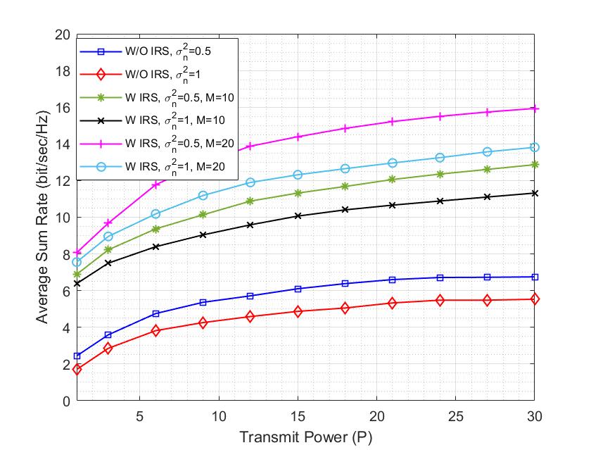
Figure 4: Average sum-rate vs. $P$; Comparison between NOMA with and without IRS in a perfect CSI scenario.

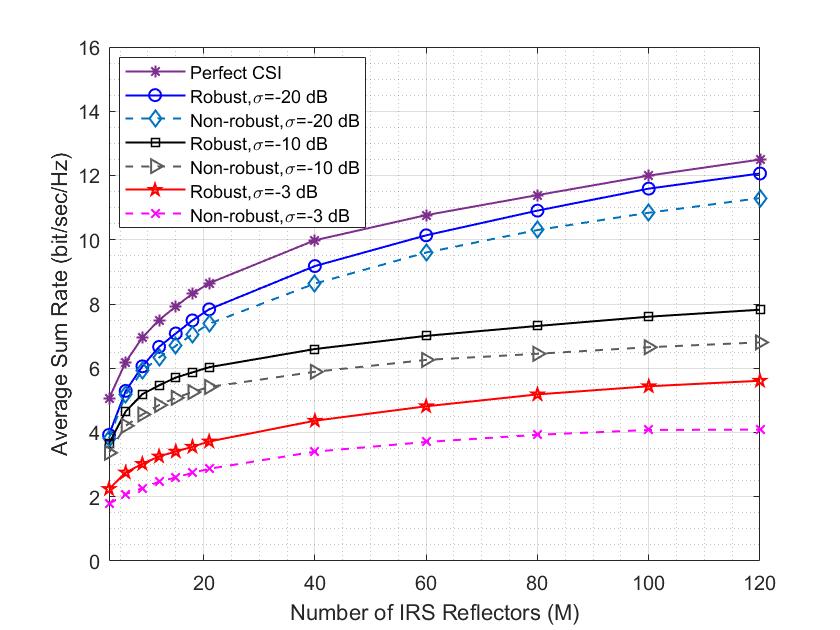
Figure 5: Average sum-rate vs. $M$; Comparison among robust, non-robust and perfect CSI designs.

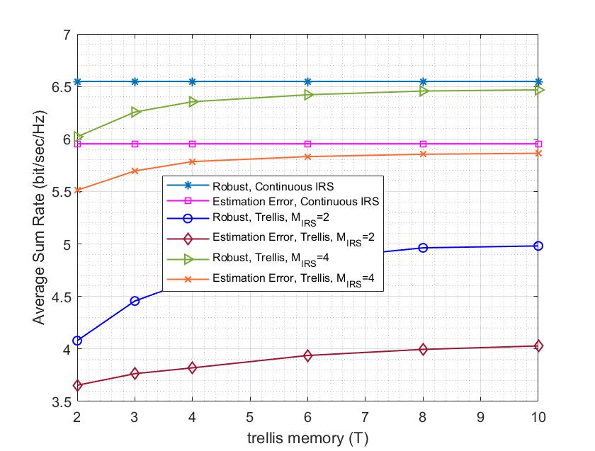
Figure 6: The average sum-rate vs. $T$, for $M=40$ and $M_{IRS}=[2,4]$.

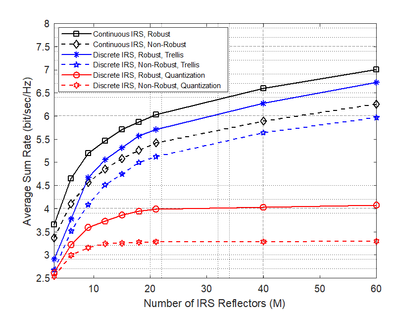
Figure 7: Average sum-rate vs. $M$; Comparison among robust, non-robust designs in $\sigma=-10dB$, for two cases of continuous and discrete phase shifters in the IRS.

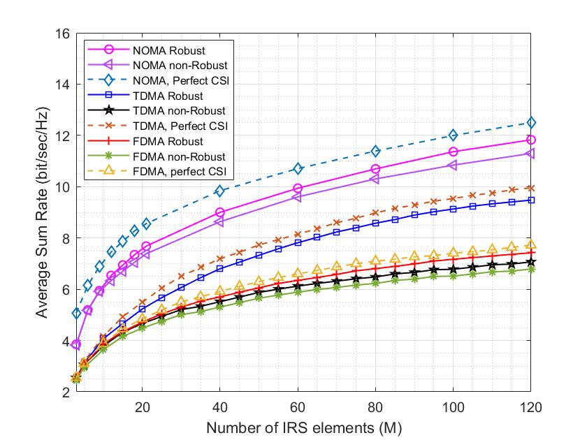
Figure 8: Average sum-rate vs. $M$; Comparison among IRS-aided FDMA, TDMA and NOMA.

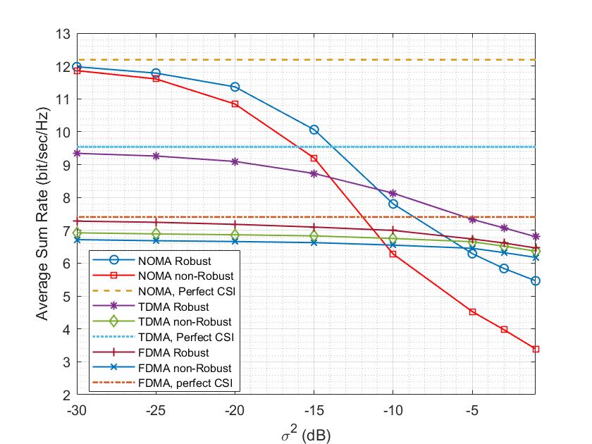
Figure 9: Average sum-rate vs. $\sigma^{2}$; Comparison among IRS-aided FDMA, TDMA and NOMA.

VII Conclusion

This paper investigates the benefit of utilizing IRS in a NOMA communication system. We attempted to jointly optimize the beamforming vector and the IRS entries under the assumption of imperfect CSI, to maximize the sum rate. The PDD algorithm is used to design a robust joint beamforming at the IRS and the AP. The proposed method is an iterative algorithm with closed-form solutions in each step, hence, the computational complexity is very low. Two cases of continuous and discrete IRS are considered in this paper, and a trellis-based solution is proposed for the discrete phase shift selection, which is shown to out-perform the conventional methods. Numerical results show the efficiency of the robust design compared to the non-robust and perfect CSI scenarios. To investigate the benefits of NOMA compared to OMA, two cases of IRS-assisted FDMA and TDMA systems are considered. It is shown that IRS-aided NOMA outperforms OMA in terms of spectral efficiency when the channel estimation error is low.

Appendix A Proof of Theorem 1

Let $\mathcal{I}\left(\alpha_{i}\mathbf{x}^{[i]};y^{[i]}|\hat{\mathbf{h}}\right)$ be the conditional mutual information of user $i$ conditioned on estimated channel matrix $\hat{\mathbf{h}}$. Expanding $\mathcal{I}\left(\alpha_{i}\mathbf{x}^{[i]};y^{[i]}|\hat{\mathbf{h}}\right)$ in terms of the differential entropies results in

$$\mathcal{I}\left(\alpha_{i}\mathbf{x}^{[i]};y^{[i]}|\hat{\mathbf{h}}\right)=\mathcal{H}\left(\alpha_{i}\mathbf{x}^{[i]}|\hat{\mathbf{h}}\right)-\mathcal{H}\left(\alpha_{i}\mathbf{x}^{[i]}|y^{[i]},\hat{\mathbf{h}}\right)$$ (71)

The first term on the right hand side of (71) simplifies to $\log_{2}\det\left(2\pi e\mathbf{v}_{i}\right),$ where $\mathbf{v}_{i}\triangleq\mathbb{E}\left\{\alpha_{i}^{2}\mathbf{x}^{[i]}\mathbf{x}^{[i]{H}}\right\}$ denotes the transmit co-variance matrix related to $\mathbf{x}^{[i]}$ [39]. Regarding the equation in (III), the second term of the right hand side of (71) is upper bounded by the entropy of a Gaussian random variable [40] as follows

$$\mathcal{H}(\alpha_{i}\mathbf{x}^{[i]}|y^{[i]},\hat{\mathbf{h}})\leq\log_{2}\det\Big{(}2\pi e(\mathbf{v}_{i}-\frac{\mathbf{v}_{i}\hat{\mathbf{h}}^{[i]H}\hat{\mathbf{h}}^{[i]}\mathbf{v}_{i}}{\hat{\mathbf{h}}^{[i]}\mathbf{v}_{i}\hat{\mathbf{h}}^{[i]H}+\Gamma_{i}})\Big{)},$$ (72)

in which

$$\Gamma_{i}\triangleq\begin{cases}\sum_{k=1}^{K}\sigma_{h}^{2}\operatorname{trace}\left(\mathbf{v}_{k}\right)+\sigma_{n}^{2},&i=1\\ \\ \hat{\mathbf{h}}^{[2]H}\mathbf{v}_{1}\hat{\mathbf{h}}^{[2]}+\sum_{k=1}^{K}\sigma_{h}^{2}\operatorname{trace}\left(\mathbf{v}_{k}\right)+\sigma_{n}^{2},&i=2.\end{cases}$$ (73)

Now, we employ the Woodbury matrix identity as follows

$$(\mathbf{A}+\mathbf{B}\mathbf{CD})^{-1}=\mathbf{A}^{-1}-\mathbf{A}^{-1}\mathbf{B}\left(\mathbf{C}^{-1}+\mathbf{D}\mathbf{A}^{-1}\mathbf{B}\right)^{-1}\mathbf{D}\mathbf{A}^{-1}.$$ (74)

Assuming $\mathbf{A}=\mathbf{I}$, $\mathbf{B}=\hat{\mathbf{h}}^{[i]H}$, $\mathbf{C}=\Gamma_{i}^{-1}$ and $\mathbf{D}=\hat{\mathbf{h}}^{[i]}\mathbf{v}_{i},$ and using (74), it is concluded

$$\mathbf{I}-\frac{\hat{\mathbf{h}}^{[i]H}\hat{\mathbf{h}}^{[i]}\mathbf{v}_{i}}{\hat{\mathbf{h}}^{[i]}\mathbf{v}_{i}\hat{\mathbf{h}}^{[i]H}+\Gamma_{i}}=\left(\mathbf{I}+\frac{\hat{\mathbf{h}}^{[i]H}\hat{\mathbf{h}}^{[i]}\mathbf{v}_{i}}{\Gamma_{i}}\right)^{-1}.$$ (75)

Thus, the right hand side of (72) can be rewritten as

$$\log_{2}\det\left(2\pi e\mathbf{v}_{i}\left(\mathbf{I}-\frac{\hat{\mathbf{h}}^{[i]H}\hat{\mathbf{h}}^{[i]}\mathbf{v}_{i}}{\hat{\mathbf{h}}^{[i]}\mathbf{v}_{i}\hat{\mathbf{h}}^{[i]H}+\Gamma_{i}}\right)\right)$$

$$=\log_{2}\det\left(2\pi e\mathbf{v}_{i}\left(\mathbf{I}+\frac{\hat{\mathbf{h}}^{[i]H}\hat{\mathbf{h}}^{[i]}\mathbf{v}_{i}}{\Gamma_{i}}\right)^{-1}\right)$$

$$=\log_{2}\det\left(2\pi e\mathbf{v}_{i}\right)-\log_{2}\det\left(\mathbf{I}+\frac{\hat{\mathbf{h}}^{[i]H}\hat{\mathbf{h}}^{[i]}\mathbf{v}_{i}}{\Gamma_{i}}\right).$$ (76)

Exploiting (A) and employing Sylvester’s determinant theorem, i. e., $\det(\mathbf{I}+\mathbf{AB})=\det(\mathbf{I}+$ BA), (72) is rewritten by

$$\mathcal{H}\left(\alpha_{i}\mathbf{x}^{[i]}|y^{[i]},\hat{\mathbf{h}}\right) \leq\log_{2}\det\left(2\pi e\mathbf{v}_{i}\left(\mathbf{I}-\frac{\hat{\mathbf{h}}^{[i]H}\hat{\mathbf{h}}^{[i]}\mathbf{v}_{i}}{\hat{\mathbf{h}}^{[i]}\mathbf{v}_{i}\hat{\mathbf{h}}^{[i]H}+\Gamma_{i}}\right)\right)$$

$$=\log_{2}\det\left(2\pi e\mathbf{v}_{i}\right)-\log_{2}\det\left(1+\frac{\hat{\mathbf{h}}^{[i]}\mathbf{v}_{i}\hat{\mathbf{h}}^{[i]H}}{\Gamma_{i}}\right).$$ (77)

Consequently, assuming $\mathbb{E}\left\{\left|s^{[i]}\right|^{2}\right\}=1$ and utilizing (A), (71) leads to

$$\mathcal{I}\left(\alpha_{i}\mathbf{x}^{[i]};y^{[i]}|\hat{\mathbf{h}}\right) \geq\log_{2}\det\left(1+\frac{\hat{\mathbf{h}}^{[i]}\mathbf{v}_{i}\hat{\mathbf{h}}^{[i]H}}{\Gamma_{i}}\right)=\log_{2}\left(1+\frac{\left|\alpha_{i}\hat{\mathbf{h}}^{[i]}\mathbf{w}_{i}\right|^{2}}{\Gamma_{i}}\right).$$ (78)

Therefore, the minimum achievable rate of the $i$-th user is written by

$$R^{[i]}=\begin{cases}\log_{2}\left(1+\frac{\alpha_{1}^{2}|\hat{\mathbf{h}}^{[1]}\mathbf{w}_{1}|^{2}}{\sigma_{h}^{2}\left(||\mathbf{w}_{1}||^{2}+||\mathbf{w}_{2}||^{2}\right)+\sigma_{n}^{2}}\right),&i=1\\ &\\ \log_{2}\left(1+\frac{\alpha_{2}^{2}|\hat{\mathbf{h}}^{[2]}\mathbf{w}_{2}|^{2}}{\alpha_{1}^{2}|\hat{\mathbf{h}}^{[2]}\mathbf{w}_{1}|^{2}+\sigma_{h}^{2}\left(||\mathbf{w}_{1}||^{2}+||\mathbf{w}_{2}||^{2}\right)+\sigma_{n}^{2}}\right),&i=2.\end{cases}$$ (79)

References

• [1] Z. Chen, Z. Ding, X. Dai, and G. K. Karagiannidis, “On the Application of Quasi-Degradation to MISO-NOMA Downlink,” IEEE Transactions on Signal Processing, vol. 64, no. 23, pp. 6174–6189, Dec 2016.
• [2] Z. Ding and H. Vincent Poor, “A Simple Design of IRS-NOMA Transmission,” IEEE Communications Letters, vol. 24, no. 5, pp. 1119–1123, May 2020.
• [3] C. Pan, H. Ren, K. Wang, J. F. Kolb, M. Elkashlan, M. Chen, M. D. Renzo, Y. Hao, J. Wang, A. L. Swindlehurst, X. You, and L. Hanzo, “Reconfigurable Intelligent Surfaces for 6G and Beyond: Principles, Applications, and Research Directions,” Nov. 2020.
• [4] C. Pan, H. Ren, K. Wang, W. Xu, M. Elkashlan, A. Nallanathan, and L. Hanzo, “Multicell MIMO Communications Relying on Intelligent Reflecting Surfaces,” IEEE Transactions on Wireless Communications (Early Access), pp. 1–1, May 2020.
• [5] C. Pan, H. Ren, K. Wang, M. Elkashlan, A. Nallanathan, J. Wang, and L. Hanzo, “Intelligent Reflecting Surface Aided MIMO Broadcasting for Simultaneous Wireless Information and Power Transfer,” IEEE Journal on Selected Areas in Communications (Early Access), pp. 1–1, June 2020.
• [6] Q. Zhang, Q. Saad, and M. Bennis, “Reflections in the sky: Millimeter wave communication with UAV-carried intelligent reflectors,” Proc. IEEE Global Commun. Conf. (GLOBECOM), Hawaii, USA, pp. 1–6, Dec 2019.
• [7] X. Yu, D. Xu, Y. Sun, D. W. K. Ng, and R. Schober, “Robust and Secure Wireless Communications via Intelligent Reflecting Surfaces,” IEEE Journal on Selected Areas in Communications, vol. 38, no. 11, pp. 2637–2652, Nov. 2020.
• [8] W. Qingqing and Z. Rui, “Weighted Sum Power Maximization for Intelligent Reflecting Surface Aided SWIPT,” IEEE Wireless Communications Letters, vol. 9, no. 5, pp. 586–590, May 2020.
• [9] J. Zuo, Y. Liu, E. Basar, and O. A. Dobre, “Intelligent Reflecting Surface Enhanced Millimeter-Wave NOMA Systems,” IEEE Communications Letters, vol. 24, no. 11, pp. 2632–2636, Nov. 2020.
• [10] Y. Omid, S. M. Shahabi, C. Pan, Y. Deng, and A. Nallanathan, “Low-Complexity Robust Beamforming Design for IRS-Aided MISO Systems with Imperfect Channels,” IEEE Communications Letters, Jan. 2021.
• [11] G. Zhou, C. Pan, H. Ren, K. Wang, M. Di Renzo, and A. Nallanathan, “Robust Beamforming Design for Intelligent Reflecting Surface Aided MISO Communication Systems,” IEEE Wireless Communications Letters ( Early Access ), pp. 1–1, June 2020.
• [12] J. Zhang, Y. Zhang, C. Zhong, and Z. Zhang, “Robust Design for Intelligent Reflecting Surfaces Assisted MISO Systems,” IEEE Communications Letters ( Early Access ), pp. 1–1, June 2020.
• [13] B. Zheng, Q. Wu, and R. Zhang, “Intelligent Reflecting Surface-Assisted Multiple Access With User Pairing: NOMA or OMA?” IEEE Communications Letters, vol. 24, no. 4, pp. 753–757, Apr 2020.
• [14] T. Hou, Y. Liu, Z. Song, X. Sun, Y. Chen, and L. Hanzo, “Reconfigurable Intelligent Surface Aided NOMA Networks,” IEEE Journal on Selected Areas in Communications, July 2020.
• [15] M. Fu, Y. Zhou, and Y. Shi, “Intelligent Reflecting Surface for Downlink Non-Orthogonal Multiple Access Networks,” 2019 IEEE Globecom Workshops (GC Wkshps), Waikoloa, HI, USA, pp. 1–6, Dec 2019.
• [16] X. Mu, Y. Liu, L. Guo, J. Lin, and N. Al-Dhahir, “Exploiting Intelligent Reflecting Surfaces in NOMA Networks: Joint Beamforming Optimization,” IEEE Transactions on Wireless Communications, vol. 19, no. 10, pp. 6884–6898, Oct. 2020.
• [17] M. Zeng, X. Li, G. Li, W. Hao, and O. A. Dobre, “Sum Rate Maximization for IRS-Assisted Uplink NOMA,” IEEE Communications Letters, vol. 25, no. 1, pp. 234–238, Jan. 2021.
• [18] Y. Cheng, K. H. Li, Y. Liu, K. C. Teh, and H. Vincent Poor, “Downlink and Uplink Intelligent Reflecting Surface Aided Networks: NOMA and OMA,” IEEE Transactions on Wireless Communications, Nov. 2021.
• [19] H. Wang, C. Liu, Z. Shi, Y. Fu, and R. Song, “On Power Minimization for IRS-Aided Downlink NOMA Systems,” IEEE Wireless Communications Letters, vol. 9, no. 11, pp. 1808–1811, Nov. 2020.
• [20] A. S. d. Sena, D. Carrillo, F. Fang, P. H. J. Nardelli, D. B. d. Costa, U. S. Dias, Z. Ding, C. B. Papadias, and W. Saad, “What Role Do Intelligent Reflecting Surfaces Play in Multi-Antenna Non-Orthogonal Multiple Access?” IEEE Wireless Communications, vol. 27, no. 5, pp. 24–31, Oct. 2020.
• [21] F. Fang, Y. Xu, Q. V. Pham, and Z. Ding, “Energy-Efficient Design of IRS-NOMA Networks,” IEEE Transactions on Vehicular Technology, vol. 69, no. 11, pp. 14 088–14 092, Nov. 2020.
• [22] Z. Ding, R. Schober, and H. V. Poor, “On the Impact of Phase Shifting Designs on IRS-NOMA,” IEEE Wireless Communications Letters, vol. 9, no. 10, pp. 1596–1600, Oct. 2020.
• [23] Y. Li, M. Jiang, Q. Zhang, and J. Qin, “Joint Beamforming Design in Multi-Cluster MISO NOMA Intelligent Reflecting Surface-Aided Downlink Communication Networks,” Sep 2019.
• [24] H. Liu, X. Yuan, and Y. A. Zhang, “Matrix-Calibration-Based Cascaded Channel Estimation for Reconfigurable Intelligent Surface Assisted Multiuser MIMO,” IEEE Journal on Selected Areas in Communications ( Early Access ), pp. 1–1, July 2020.
• [25] G. Zhou, C. Pan, H. Ren, K. Wang, and A. Nallanathan, “A Framework of Robust Transmission Design for IRS-aided MISO Communications with Imperfect Cascaded Channels,” jan 2020. [Online]. Available: http://arxiv.org/abs/2001.07054
• [26] Q. Shi and M. Hong, “Penalty Dual Decomposition Method For Nonsmooth Nonconvex Optimization—Part I: Algorithms and Convergence Analysis,” IEEE Transactions on Signal Processing, vol. 68, pp. 4108–4122, June 2020.
• [27] M. Razaviyayn, M. Hong, and Z. Luo, “A unified convergence analysis of block successive minimization methods for nonsmooth optimization,” SIAM Journal on Optimization, vol. 32, no. 2, p. 1126–1153, 2013.
• [28] Q. Wu and R. Zhang, “Intelligent Reflecting Surface Enhanced Wireless Network via Joint Active and Passive Beamforming,” IEEE Transactions on Wireless Communications, vol. 18, no. 11, pp. 5394 – 5409, Nov 2019.
• [29] X. Yu, D. Xu, and R. Schober, “Enabling Secure Wireless Communications via Intelligent Reflecting Surfaces,” in 2019 IEEE Global Communications Conference (GLOBECOM).   IEEE, 2019, pp. 1–6.
• [30] C. Huang, A. Zappone, G. C. Alexandropoulos, M. Debbah, and C. Yuen, “Reconfigurable Intelligent Surfaces for Energy Efficiency in Wireless Communication,” oct 2018.
• [31] Z. Abdullah, G. Chen, S. Lambotharan, and J. A. Chambers, “Optimization of Intelligent Reflecting Surface Assisted Full-Duplex Relay Networks,” IEEE Wireless Communications Letters (Early Access).
• [32] ——, “A Hybrid Relay and Intelligent Reflecting Surface Network and Its Ergodic Performance Analysis,” IEEE Wireless Communications Letters, vol. 9, no. 10, pp. 653–1657, Oct. 2020.
• [33] T. Hou, Y. Liu, Z. Song, X. Sun, Y. Chen, and L. Hanzo, “MIMO Assisted Networks Relying on Large Intelligent Surfaces: A Stochastic Geometry Model,” Oct 2019.
• [34] Y. Liu, G. Pan, H. Zhang, and M. Song, “On the Capacity Comparison Between MIMO-NOMA and MIMO-OMA,” IEEE Access, vol. 4, pp. 2123–2129, May. 2016.
• [35] Q. Shi, M. Hong, X. Fu, and T. Chang, “Penalty Dual Decomposition Method For Nonsmooth Nonconvex Optimization—Part II: Applications,” IEEE Transactions on Signal Processing ( Early Access ), pp. 1–1, June 2020.
• [36] M. Kazemi, H. Aghaeinia, and T. M. Duman, “Discrete-Phase Constant Envelope Precoding for Massive MIMO Systems,” IEEE Transactions on Communications, vol. 65, no. 5, pp. 2011–2021, may 2017.
• [37] Y. Omid, S. M. M. Shahabi, C. Pan, Y. Deng, and A. Nallanathan, “A Trellis-based Passive Beamforming Design for an Intelligent Reflecting Surface-Aided MISO System,” IEEE Communications Letters, March 2022.
• [38] 3GPP, “Technical specification group radio access network; 3GPP TR 25.996, Spatial channel model for MIMO simulations,,” vol. 1, no. Release 10, 2011.
• [39] T. M. Cover and J. A. Thomas, Elements of Information Theory, ser. Wiley Series in Telecommunications.   New York, USA: John Wiley & Sons, Inc., 1991.
• [40] M. Medard, “The effect upon channel capacity in wireless communications of perfect and imperfect knowledge of the channel,” IEEE Transactions on Information Theory, vol. 46, no. 3, pp. 933–946, may 2000.