Revisiting the pion Regge trajectories

Abstract

We propose a model-independent ansatz $M={\beta_{x}}\left(x+c_{0}\right)^{\nu}+c_{1}$ ($x=l,\,n_{r}$) and then use it to fit the orbital and radial pion Regge trajectories without the preset values. It is shown that nonzero $c_{1}$ is reasonable and acceptable. Nonzero $c_{1}$ gives an explanation for the nonlinearity of the pion Regge trajectories in the usually employed $(M^{2},\,x)$ plane. As $m_{R}$ or $c_{1}$ is chosen appropriately, both the orbital and radial pion Regge trajectories are linear in the $((M-m_{R})^{2},\,x)$ plane whether the $\pi^{0}$ is included or not on the Regge trajectories. The fitted pion Regge trajectories suggest $0.45\leq\nu\leq 0.5$, which indicates the confining potential $r^{a}$ with $9/11{\leq}a\leq 1$. Moreover, it is illustrated in the appendix B that $m_{R}$ can be nonzero for the light nonstrange mesons. We present discussions in the appendix A on the structure of the Regge trajectories plotted in the $(M,\,x)$ plane and on the structure of the Regge trajectories in the $((M-m_{R})^{2},\,x)$ plane based on the potential models and the string models.

I Introduction

Understanding the spectrum of hadrons reveals information on the non-perturbative aspects of QCD Godfrey:1998pd and on the inner structure of hadrons. The Regge trajectory is one of the effective approaches for studying hadron spectra Regge:1959mz ; Collins:1971ff ; Chew:1961ev ; Hey:1982aj ; Inopin:2001ub ; Chen:2016spr ; Chen:2016qju ; Inopin:1999nf ; Chew:1962eu ; Brodsky:2017qno . The orbital and radial Regge trajectories note for pion are often taken as being approximately linear in the $(M^{2},\,l)$ plane and in the $(M^{2},\,n_{r})$ plane, respectively, $M^{2}={\alpha_{1}}l+{\alpha_{2}}n_{r}+c$ Anisovich:2000kxa ; Afonin:2006vi ; Shifman:2007xn ; Ebert:2009ub ; Masjuan:2012gc ; Kobzarev:1992wt ; Lucha:1991ce ; Afonin:2021cwo , where $M$ is the mass, $\alpha_{1}$ and $\alpha_{2}$ are the Regge slopes, $l$ is the orbital angular momentum, $n_{r}$ is the radial quantum number, and $c$ is a constant. The pion Regge trajectories are in fact nonlinear when they are examined more precisely, see Fig. 1. Many authors have discussed the nonlinearity of the pion Regge trajectories. In Ref. Tang:2000tb , the authors note that the orbital pion Regge trajectory is nonlinear by the ”zone test”, $M^{2}=-0.1077J^{2}+1.6003J+0.019$, where $J$ is the total angular momentum. In Ref. Brisudova:1999ut , the pion Regge trajectory is discussed by using the square-root trajectory. In Ref. Sharov:2013tga , the author gives the nonlinear pion orbital Regge trajectory with corrections based on the string model. In Ref. Sonnenschein:2014jwa , the pion Regge trajectory is nonlinear as the masses of quarks are considered. In Refs. Chen:2021kfw ; Chen:2018hnx ; Chen:2018bbr , the pion Regge trajectories are fitted by a nonlinear formula, $M^{2}=2.78(0.8+n_{r})^{2/3}-2.38$. It is known that the significant nonlinearity of the Regge trajectories for the heavy mesons arises from the nonrelativisity of heavy mesons Sergeenko:1994ck ; Inopin:1999nf ; Sonnenschein:2018fph ; Sonnenschein:2014jwa ; Cotugno:2009ys ; Burns:2010qq ; Kruczenski:2004me ; MartinContreras:2020cyg ; Chen:2021kfw ; Chen:2018hnx ; Chen:2018nnr ; Chen:2018bbr due to the heavy masses of quarks. In this work, we revisit the pion Regge trajectories and present discussions on the nonlinearity of them.

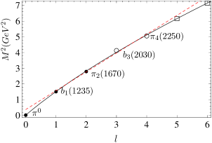
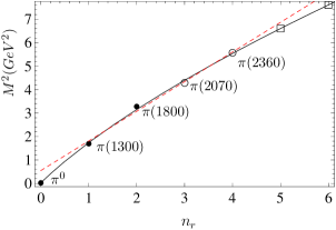
Figure 1: The fitted orbital and radial Regge trajectories for pion, which are plotted in the $(M^{2},\,l)$ plane and in the $(M^{2},\,n_{r})$ plane, respectively. These figures are from Ref. Chen:2021kfw . The well-established states are given by solid dots and the unwell-established states are given by circles. Open squares are predicted masses.

This paper is organized as follows: In Sec. II, we fit the orbital and radial pion Regge trajectories by using four points and five points on the Regge trajectories, respectively. The discussions are presented in Sec. III and the conclusions are in Sec. IV.

II Fit of the pion Regge trajectories

In this section, we fit the orbital and radial Regge trajectories for the pion by employing a newly proposed ansatz. The ansatz is model-independent and therefore the fit is model-independent. Then we obtain the fitted parameters without the preset values.

II.1 Preliminaries

The Regge trajectories can be written in different forms, such as $l=l(M)$, $M^{2}=f(l,\,n_{r})$, $M=M(l,\,n_{r})$ Burns:2010qq , $(M-m)^{2}=g(l,\,n_{r})$ Afonin:2020bqc ; Chen:2017fcs ; Jia:2019bkr and so on. We use the following ansatz inspired by Refs. Chen:2021kfw ; MartinContreras:2020cyg ; Brau:2000st

$$M={\beta_{x}}\left(x+c_{0}\right)^{\nu}+c_{1}\;\;(x=l,\,n_{r})$$ (1)

to fit the orbital and radial Regge trajectories note for the pion in the $(M,\,x)$ plane. $\beta_{x}$ is the slope. The constants $c_{0}$ and $c_{1}$ vary with different Regge trajectories. The exponent $\nu$ which relates to the dynamics of mesons is regarded as a free parameter in fit. As $0<\nu<1$, $\nu=1$ or $\nu>1$, Eq. (1) becomes concave downwards, linear or convex upwards, respectively. $\nu\in(0,1)$ is used to find the appropriate value because the pion orbital and radial Regge trajectories are obviously concave in the $(M,\,n_{r})$ and $(M,\,l)$ planes, see Fig. 4.

The used data are listed in the 3rd column in Table 1. The quality of a fit is measured by the quantity $\chi^{2}$ defined by Sonnenschein:2014jwa

$$\chi^{2}=\frac{1}{N-1}\sum_{i=1}^{N}\left(\frac{M_{fi}-M_{ei}}{M_{ei}}\right)^{2},$$ (2)

where $N$ is the number of points on the trajectory, $M_{fi}$ is the fitted value and $M_{ei}$ is the experimental value of the $i$-th particle.

The fit is calculated by using MATHEMATICA program. $c_{0}$, $c_{1}$ and $\nu$ are free parameters. $\beta_{x}$ is calculated by using the FindFit function and Eq. (1). The quantity $\chi^{2}$ is calculated by using Eq. (2). By minimizing the $\chi^{2}$ quantity for a given $\nu$, the parameters $c_{0}$, $c_{1}$ and $\beta_{x}$ are determined for each value of $\nu$.

Table 1: Mesons’ masses (in units of ${\rm MeV}$). The experimental masses are from PDG ParticleDataGroup:2020ssz . The fitted results by using the Regge trajectories [Eq. (1)] are shown in comparison with the theoretical values in the EFG model Ebert:2009ub and in the GI model Godfrey:1985xj . Fit5 are obtained by using five points on the Regge trajectories while Fit4 are fitted by excluding $\pi^{0}$. A question mark ($?$) indicates an unwell-established state. The fitted Regge trajectories are listed in Table 2.

State	Meson	PDG ParticleDataGroup:2020ssz	EFG Ebert:2009ub	GI Godfrey:1985xj	Fit5			Fit4
					$\nu=0.4$	$\nu=0.45$	$\nu=0.5$	$\nu=0.4$	$\nu=0.45$	$\nu=0.5$
$1^{1}S_{0}$	$\pi^{0}$	$134.9768\pm 0.0005$	154	150	135	136	135	$-$115	90	255
$2^{1}S_{0}$	$\pi(1300)$	$1300\pm 100$	1292	1300	1307	1302	1269	1310	1312	1315
$3^{1}S_{0}$	$\pi(1800)$	$1810^{+9}_{-11}$	1788	1880	1764	1756	1739	1765	1759	1754
$4^{1}S_{0}$	$\pi(2070)$?	$2070\pm 35$	2073		2096	2095	2099	2096	2093	2091
$5^{1}S_{0}$	$\pi(2360)$?	$2360\pm 25$	2385		2368	2376	2403	2366	2370	2375
$6^{1}S_{0}$					2601	2621	2671	2598	2611	2625
$7^{1}S_{0}$					2808	2840	2913	2803	2827	2851
$8^{1}S_{0}$					2995	3039	3135	2989	3023	3060
$1^{1}S_{0}$	$\pi^{0}$	$134.9768\pm 0.0005$	154	150	135	135	135	$-$175	25	185
$1^{1}P_{1}$	$b_{1}(1235)$	$1229.5\pm 3.2$	1258	1220	1226	1235	1213	1229	1231	1232
$1^{1}D_{2}$	$\pi_{2}(1670)$	$1670.6^{+2.9}_{-1.2}$	1643	1680	1675	1673	1660	1678	1672	1666
$1^{1}F_{3}$	$b_{3}(2030)$?	$2032\pm 12$	1884	2030	2004	2000	2002	2004	2002	1998
$1^{1}G_{4}$	$\pi_{4}(2250)$?	$2250\pm 15$	2092	2330	2272	2272	2291	2270	2275	2279
$1^{1}H_{5}$					2502	2508	2545	2498	2513	2526
$1^{1}I_{6}$					2707	2719	2776	2700	2726	2750

Table 2: The fitted pion Regge trajectories (in units of ${\rm GeV}$) by using four points (Fit4) and by using five points (Fit5).

		Fit4		Fit5
		Traj.	$\chi^{2}$	Traj.	$\chi^{2}$
	$\nu=0.4$	$M=1.404\,l^{0.4}-0.175$	$9.5\times 10^{-5}$	$M=1.424(l+0.03)^{0.4}-0.215$	$7.7\times 10^{-5}$
Orbital Traj.	$\nu=0.45$	$M=1.206\,l^{0.45}+0.025$	$1.15\times 10^{-4}$	$M=1.198(l+0.004)^{0.45}+0.035$	$9.0\times 10^{-5}$
	$\nu=0.5$	$M=1.047\,l^{0.5}+0.185$	$1.5\times 10^{-4}$	$M=1.078\,l^{0.5}+0.135$	$1.9\times 10^{-4}$
	$\nu=0.4$	$M=1.425\,n_{r}^{0.4}-0.115$	$2.8\times 10^{-4}$	$M=1.438(n_{r}+0.016)^{0.4}-0.14$	$2.2\times 10^{-4}$
Radial Traj.	$\nu=0.45$	$M=1.222\,n_{r}^{0.45}+0.09$	$3.4\times 10^{-4}$	$M=1.241(n_{r}+0.002)^{0.45}+0.06$	$2.8\times 10^{-4}$
	$\nu=0.5$	$M=1.060\,n_{r}^{0.5}+0.255$	$4.1\times 10^{-4}$	$M=1.134\,n_{r}^{0.5}+0.135$	$6.7\times 10^{-4}$

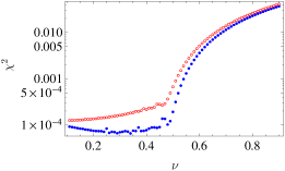
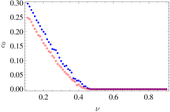
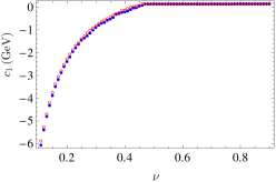
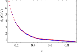
Figure 2: The quantities $\chi^{2}$, $c_{1}$, $c_{0}$ and $\beta_{x}$ ($x=l,\,n_{r}$) vary with different exponent $\nu$. The orbital Regge trajectory (the blue dots) and the radial Regge trajectory (the red circles) are fitted by using five points on the Regge trajectories, that is, $\pi^{0}$ is included in fit. The used formulas are Eqs. (1) and (2).

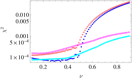
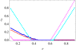
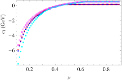
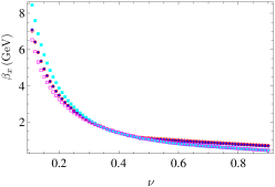
Figure 3: Comparison between the fitted quantities $\chi^{2}$, $c_{1}$, $c_{0}$ and $\beta_{x}$. The quantities which are obtained from the fitted orbital (the blue dots) and radial (the red circles) Regge trajectory as the pion is included (five-point fit) are compared with the quantities obtained from the fitted orbital (the cyan solid squares) and radial (the magenta empty squares) Regge trajectory as the $\pi^{0}$ is excluded (four-point fit). The used formulas are Eqs. (1) and (2).

II.2 Fit of the pion Regge trajectories by using five points

In this subsection, the $\pi^{0}$ is included in fit, that is, five points or five states listed in Table 1 are used to fit the orbital and radial Regge trajectories by employing Eq. (1), respectively.

The quantities $\chi^{2}$, $c_{1}$, $c_{0}$ and $\beta_{l}$ ($\beta_{n_{r}}$) vary with the exponent $\nu$, see Fig. 2. $\nu$ ranges from $0.1$ to $0.9$ because as ${\nu}{\gtrapprox}1$, the fitted values of $c_{0}$ and $c_{1}$ become anomalous and omitting $\nu\in(0.9,1)$ does not affect the results. $\chi^{2}$ increases with $\nu$. It increases rapidly and becomes large as $\nu{\gtrapprox}0.5$, see Fig. 2. $c_{0}$ is related with the curvature of the used formula (1). $c_{0}>0$ implies that the curvature of the formula (1) may be larger than expected while $c_{0}=0$ suggests that the exponent $\nu$ is appropriate or large. As shown in Fig. 2, the fitted results prefer $0<\nu{\lessapprox}0.46$. $c_{1}$ is expected to be greater than or equal to $0$, see the appendix A.2 and Eq. (35). The $c_{1}-\nu$ plot shows that the better value is $\nu{\gtrapprox}0.43$, see 2. As $\nu\in(0.45,\,0.6)$, $\beta_{l}^{2}\in(1.436,\,0.942)$ and $\beta_{n_{r}}^{2}\in(1.54,\,1.04)$, see Fig. 2. According to the previous discussions, for the five-point fit $\nu\approx 0.45$ is the better fitted value without considering the Regge slopes.

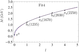
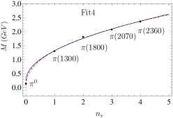
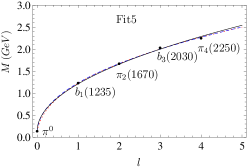
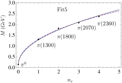
Figure 4: The fitted orbital and radial Regge trajectories for pion by using four points (Fit4) and by using five points (Fit5). They are plotted in the $(M,\,l)$ plane and in the $(M,\,n_{r})$ plane, respectively. The red dotted lines are for $\nu=0.4$, the blue dashed lines are for $\nu=0.45$ and the black lines are for $\nu=0.5$. The used formulas are listed in Table 2.

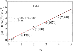
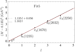
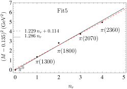
Figure 5: The fitted orbital and radial Regge trajectories for pion by using 4 points (Fit4) and by using 5 points (Fit5). They are plotted in the $((M-m_{R})^{2},\,l)$ plane and in the $((M-m_{R})^{2},\,n_{r})$ plane, respectively. The used formulas for the black lines are from Table 2. The red dashed lines are the linear fits.

The fitted Regge trajectories by using five points are listed in Table 2 with $\nu=0.4,\,0.45,\,0.5$. They are plotted in the $(M,\,l)$ plane and in the $(M,\,n_{r})$ plane, respectively, see Fig. 4. The fitted masses are listed in Table 1, which are in agreement with the experimental values.

As mentioned in the introduction, the pion Regge trajectories are nonlinear in the $(M^{2},\,x)$ ($x=l,\,n_{r}$) plane, see Fig. 1. However, both of the orbital pion Regge trajectory and the radial pion Regge trajectory can be described in a linear form when they are plotted in the $((M-m_{R})^{2},\,x)$ plane with appropriate $m_{R}$, see Fig. 5.

II.3 Fit of the pion Regge trajectories by using four points

The pion can be explained as the pseudo-Nambu-Goldstone boson associated with chiral symmetry breaking Horn:2016rip ; Sonnenschein:2018fph . The low-mass pion is often excluded from the corresponding Regge trajectories formed by its orbitally or radially excited partners. In this subsection, we fit the orbital and radial Regge trajectories formed by the four orbitally excited states of $\pi^{0}$ and by the four radially excited states of $\pi^{0}$, respectively.

$\chi^{2}$ for the orbital and radial Regge trajectories increases with the exponent $\nu$. $\chi^{2}$ obtained by using the four points is roughly equal to $\chi^{2}$ calculated by using the five points as $\nu\in(0,0.5)$, see Fig. 3. According to Fig. 3, $\nu\in(0.39,\,0.64)$ for the orbital Regge trajectory and $\nu\in(0.15,\,0.6)$ for the radial Regge trajectory as $c_{0}=0$. $c_{1}$ and $\beta_{x}$ calculated by four points have similar behavior as that obtained by using five points, respectively. In the range $\nu\in(0.3,0.5)$, $c_{1}$ (or $\beta_{x}$) obtained by using four points and five points are approximately equal. As shown in Fig. 3, $\nu{\gtrapprox}0.43$ for the radial Regge trajectory and $\nu{\gtrapprox}0.45$ for the orbital Regge trajectory as $c_{1}\geq 0$. As $\nu\in(0.45,\,0.6)$, $\beta_{l}^{2}\in(1.454,\,0.659)$ and $\beta_{n_{r}}^{2}\in(1.493,\,0.677)$, see Fig. 3. We can conclude that the better value of $\nu$ ranges from 0.45 to 0.5 for the four-point fit.

When $\pi^{0}$ is excluded in fit, the fitted Regge trajectories by using 4 points with $\nu=0.4,\,0.45,\,0.5$ agree well with the experimental values, see Table 2. The extrapolated masses of $\pi^{0}$ from the fitted radial Regge trajectories are $-115$ ${\rm MeV}$, $90$ ${\rm MeV}$ and $255$ ${\rm MeV}$ for $\nu=0.4,\,0.45,\,0.5$, respectively. For the orbital Regge trajectory, the extrapolated masses of $\pi^{0}$ are $-175$ ${\rm MeV}$, $25$ ${\rm MeV}$ and $185$ ${\rm MeV}$ for $\nu=0.4,\,0.45,\,0.5$, respectively. The fitted pion Regge trajectories are plotted in the $(M,\,l)$ plane and in the $(M,\,n_{r})$ plane, respectively, see Fig. 4. Whether the $\pi^{0}$ is included or not, both the orbital Regge trajectory and the radial Regge trajectory are linear when they are plotted in the $((M-m_{R})^{2},\,x)$ plane with nonzero $m_{R}$, see Fig. 5. For the five-point fit, $m_{R}=135$ ${\rm MeV}$ for both the orbital Regge trajectory and the radial Regge trajectory, which is the experimental value of $\pi^{0}$. But for the four-point fit, $m_{R}=255$ ${\rm MeV}$ for the radial Regge trajectory and $m_{R}=185$ ${\rm MeV}$ for the orbital Regge trajectory in case of $\nu=0.5$.

III Discussions

III.1 Confining potentials

The confining potentials taking the power-law form with different power indexes are discussed in many works, such as $V_{conf}{\sim}r$ in the well-known Cornell potential Eichten:1974af , $V_{conf}{\sim}r^{0.91}$ Flamm:1987kx , $V_{conf}{\sim}r^{3/4}$ Lichtenberg:1988tn , $V_{conf}{\sim}r^{2/3}$ Heikkila:1983wd ; song:1991jg , $V_{conf}{\sim}r^{1/2}$ Song:1986ix , $V_{conf}{\sim}r^{0.1}$ Martin:1980jx ; Martin:1980rm and so on. In Ref. Rai:2008sc , the mass spectrums are extracted and the radial wave functions are reproduced from different models as well as from the nonrelativistic phenomenological quark antiquark potential of the type $V(r)=-\alpha_{s}/r+Ar^{\delta}$ with $\delta$ varying from 0.5 to 2. In Ref. Patel:2008na , the power index range of $0.1<\delta<2.0$ has been explored when computing the decay rates and spectroscopy of the $Q\bar{Q}$ mesons in the nonrelativistic potential.

The exponent $\nu$ in (1) is related to the confining potential, see Eq. (19) and the appendix A.1.1. In case of the ultrarelativistic energy region, $\nu=1/2$ indicates the linear confining potential, $V_{conf}{\sim}r$. $\nu=0.45$ implies $V_{conf}{\sim}r^{9/11}$. $\nu=0.4$ arises from the confining potential $V_{conf}{\sim}r^{2/3}$. In case of the nonrelativistic energy region, $\nu=1/2,\,0.45,\,0.4$ give $V_{conf}{\sim}r^{a}$ with $a=2/3,\,18/31,\,1/2$, respectively. It is known that the orbitally excited states and the radially excited states of pion are taken as the ultrarelativistic systems Chen:2021kfw . The suggested $0.45\leq\nu\leq 0.5$ by the fit indicates the confining potential $r^{a}$ with $9/11{\leq}a\leq 1$.

III.2 Parameter $c_{1}$ or $m_{R}$

In the ultrarelativistic limit, $c_{1}$ in (1) or $m_{R}$ in (34) is usually assumed to be zero, i.e., the Regge trajectory takes the form $M^{2}={\alpha_{x}}(x+c_{0})^{\gamma}$ with $\gamma=1$. According to Eqs. (3), (26), (34), (35), (24) and (25), $c_{1}$ or $m_{R}$ is related with the masses of constituents and the constant part of the interaction energy, especially in the nonrelativistic energy region. In Ref. Godfrey:1985xj , $m_{u}=m_{d}=220$ ${\rm MeV}$, $C$ in Eq. (5) reads $C=-253$ ${\rm MeV}$. Substituting $m_{u}$, $m_{d}$ and $\epsilon_{c}=C$ into Eq. (35) gives $c_{1}=m_{R}=187$ ${\rm MeV}$. It is in excellent agreement with $185$ ${\rm MeV}$ which is obtained from the fitted orbital Regge trajectories ($\nu=0.5$) and is smaller than $255$ ${\rm MeV}$ which is from the fitted radial Regge trajectories ($\nu=0.5$) as $\pi^{0}$ is excluded in fit, see Table 2.

As shown in the appendix B, nonzero $m_{R}$, i.e., nonzero $c_{1}$ in Eq. (1) will shift the slope of the Regge trajectories to a lower value. They can give the reasonable slopes. It shows that nonzero $c_{1}$ or nonzero $m_{R}$ is appropriate and acceptable.

It is the nonzero $c_{1}$ or $m_{R}$ together with $\beta_{x}(x+c_{0})^{1/2}$ that leads to the nonlinearity of the orbital $(M^{2},\,l)$ pion Regge trajectory and the nonlinearity of the radial $(M^{2},\,n_{r})$ pion Regge trajectory. As $m_{R}$ is not equal to zero and is chosen appropriately, the radial pion Regge trajectory in the $((M-m_{R})^{2},\,n_{r})$ plane and the orbital Regge trajectory in the $((M-m_{R})^{2},\,l)$ plane are linear whether the $\pi^{0}$ is included on the Regge trajectories, see Fig. 5.

According to Eq. (1) or (34), $c_{1}{\neq}0$ [or $m_{R}{\neq}0$] means that one part of $M$ keeps constant and does not vary with $l$ and $n_{r}$ while the other portion changes with $l$ or $n_{r}$. $c_{1}=0$ [or $m_{R}=0$] implies that all parts of the bound-state masses are effected by the potentials because $\nu$ is related with the confining potential. $c_{0}=0$ indicates that $M$ varies with $l$ or $n_{r}$ in a simple way. As $c_{0}{\neq}0$, $c_{0}$ will be entangled with $l$ ($n_{r}$) because $\nu{\neq}1$.

III.3 A note on $\pi^{0}$

There are lots of discussions on the intrinsic structure of the pion Horn:2016rip ; Arrington:2021biu ; Fariborz:2021gtc . In Ref. Alexandrou:2017itd , the lattice QCD gives $m_{\pi}=296$ ${\rm MeV}$. In Ref. Santowsky:2021ugd , $m_{\pi}=328$ ${\rm MeV}$. In Ref. Frezzotti:2022dwn , the pion mass is in the range $250-500$ ${\rm MeV}$. The extrapolated mass are $m_{\pi}=185$ ${\rm MeV}$ for the orbital Regge trajectory by using four points and $m_{\pi}=255$ ${\rm MeV}$ for the radial Regge trajectory by using four points in case of the linear confining potential. They are larger than the experimental result and smaller than the results in Refs. Alexandrou:2017itd ; Santowsky:2021ugd . According to the discussions in section II, it is not foreclosed and reasonable that $\pi^{0}$ is taken as the first point on the pion Regge trajectories, see Figs. 4, 4, 5 and 5. It implies that $\pi^{0}$ can be regarded as the quark-antiquark state like other states on the pion Regge trajectories.

IV Conclusions

The orbital and radial pion Regge trajectories are fitted phenomenologically by employing the ansatz $M={\beta_{x}}\left(x+c_{0}\right)^{\nu}+c_{1}$ where $x=l,\,n_{r}$. It is shown that nonzero $m_{R}$ is reasonable and acceptable. Nonzero $m_{R}$ or $c_{1}$ gives an explanation that the pion Regge trajectories are concave in the usually employed $(M^{2},\,x)$ plane as being examined more precisely. As $m_{R}$ is chosen appropriately, both the orbital and radial pion Regge trajectories are linear in the $((M-m_{R})^{2},\,x)$ plane whether the $\pi^{0}$ is included or not on the Regge trajectories. It is reasonable and not foreclosed that $\pi^{0}$ is regarded as the first point on the pion Regge trajectories. The fitted pion Regge trajectories suggest $0.45\leq\nu\leq 0.5$. It indicates the confining potential $r^{a}$ with $9/11{\leq}a\leq 1$.

We present discussions in the appendix A on the structure of the Regge trajectories plotted in the $(M,\,x)$ plane and in the $((M-m_{R})^{2},\,x)$ plane based on the potential models and the string models. In the appendix B, the Regge trajectories for the light nonstrange mesons with different $m_{R}$ are shown in the $((M-m_{R})^{2},\,x)$ plane. It is illustrated that $m_{R}$ can be nonzero for the light nonstrange mesons.

Appendix A Structure of the Regge trajectories

The potential models are the basic tools of the phenomenological approach to model the features of QCD relevant to hadron with the aim to produce concrete results. In Ref. Chen:2021kfw , we present discussions on the structure of the meson Regge trajectories plotted in the $(M^{2},\,x)$ plane where $x=n_{r},\,l$ based on the quadratic form of the spinless Salpeter-type equation Baldicchi:2007ic ; Baldicchi:2007zn ; Brambilla:1995bm ; chenvp ; chenrm . Herein, we present discussions on the structure of the meson Regge trajectories plotted in the $(M,\,x)$ plane and in the $((M-m_{R})^{2},\,x)$ plane note .

A.1 Structure of the Regge trajectories in the $(M,\,x)$ plane

A.1.1 Potential models

The relativistic quark model or the Godfrey-Isgur (GI) model is employed. The spin-dependent interactions are not considered. The dynamic equation is the spinless Salpeter equation (SSE) Durand:1981my ; Durand:1983bg ; Lichtenberg:1982jp ; Godfrey:1985xj ; Jacobs:1986gv which reads

$$M\Psi({{\bf r}})=\left(\omega_{1}+\omega_{2}\right)\Psi({{\bf r}})+V\Psi({{\bf r}}),$$ (3)

where $M$ is the bound state mass, $\omega_{i}$ is the square-root operator of the relativistic kinetic energy of constituent

$$\omega_{i}=\sqrt{m_{i}^{2}+{\bf p}^{2}}=\sqrt{m_{i}^{2}-\Delta},$$ (4)

$m_{1}$ and $m_{2}$ are the effective masses of the constituents, respectively. In the present work, the Cornell potential Eichten:1974af is considered,

$$V(r)=-\frac{\alpha}{r}+{\sigma}r+C,$$ (5)

where $\sigma$ is the string tension. $\alpha=4\alpha_{s}/3$ and $\alpha_{s}$ is the strong coupling constant of the color Coulomb potential. $C$ is a parameter which is fundamental and indispensable as the quark masses, slope of the linear potential $\sigma$, and the strong coupling constant. $C{\approx}-2\sqrt{\sigma}\exp[-\gamma_{E}+1/2]$ Gromes:1981cb ; Lucha:1991vn where $\gamma_{E}$ is the Euler constant.

In the nonrelativistic (NR) region, $m_{1},m_{2}{\gg}{{|\bf p|}}$, we can obtain from Eq. (3)

$$M\Psi({{\bf r}})=\left(m_{1}+m_{2}+\frac{{\bf p}^{2}}{2\mu}\right)\Psi({{\bf r}})+V\Psi({{\bf r}}),$$ (6)

where $\mu=m_{1}m_{2}/(m_{1}+m_{2})$. By employing the Bohr-Sommerfeld quantization approach Brau:2000st ; brsom , we obtain from Eq. (6)

$$M{\sim} \frac{3}{2}\left(\frac{\sigma^{2}}{\mu}\right)^{1/3}l^{2/3}\quad(l{\gg}n_{r}),$$

$$M{\sim} \left(\frac{3\pi}{2}\right)^{2/3}\left(\frac{\sigma^{2}}{2\mu}\right)^{1/3}n_{r}^{2/3}\quad(n_{r}{\gg}l).$$ (7)

In the ultrarelativistic (UR) region, ${{|\bf p|}}{\gg}m_{1},m_{2}$, we can obtain from Eq. (3)

$$M\Psi({{\bf r}})=2{{|\bf p|}}\Psi({{\bf r}})+V\Psi({{\bf r}}).$$ (8)

Then we have from Eq. (8)

$$M{\sim} 2\sqrt{2\sigma}\sqrt{l}\quad(l{\gg}n_{r}),$$

$$M{\sim} 2\sqrt{{\pi}\sigma}\sqrt{n_{r}}\quad(n_{r}{\gg}l).$$ (9)

Both of Eqs. (A.1.1) and (A.1.1) have been obtained in Ref. Brau:2000st .

If one or both of the constituents are in the intermediate (IM) energy region, $m_{i}{\sim}{{|\bf p|}}$ or $m_{1},m_{2}{\sim}{{|\bf p|}}$. According to the author’s knowledge, the approximated form of $M$ has not been obtained due to its complexity. If there is a simple approximation

$$M{\sim}x^{\nu}\quad(x=l,\,n_{r}),$$ (10)

$\nu$ is expected to lie between $1/2$ and $2/3$ MartinContreras:2020cyg .

Based on Eqs. (6), (A.1.1), (8), (A.1.1) and (10), we can propose a generic form of a Regge trajectory which has the same form as the new ansatz in Eq. (1). If the confining potential is linear, $V_{conf}={\sigma}r$, the theoretical values of the exponent $\nu$ read

$$\left\{\begin{array}[]{cc}\nu=\frac{2}{3},&\text{NR region},\\ \frac{1}{2}<\nu<\frac{2}{3},&\text{IM region},\\ \nu=\frac{1}{2},&\text{UR region}.\end{array}\right.$$ (14)

The plot corresponding to Eq. (14) is shown in Fig. 6. If the confining potential is the power-law potential

$$V_{conf}={\sigma}r^{a},$$ (15)

Eq. (14) becomes Brau:2000st

$$\left\{\begin{array}[]{cc}\nu=\frac{2a}{a+2},&\text{NR region},\\ \frac{a}{a+1}<\nu<\frac{2a}{a+2},&\text{IM region},\\ \nu=\frac{a}{a+1},&\text{UR region}.\end{array}\right.$$ (19)

Different forms of kinematic terms corresponding to different energy regions will yield different behaviors of the Regge trajectories Chen:2021kfw . ${\bf p}$ and $r^{a}$ leads to $M{\sim}x^{a/(a+1)}$ while ${\bf p}^{2}$ and $r^{a}$ gives $M{\sim}x^{2a/(a+2)}$ $(x=l,\,n_{r})$.

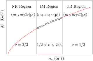
Figure 6: The structure of the Regge trajectory corresponding to different energy regions according to Eqs. (1) and (14). It is plotted in the $(M,\,x)$ plane where $x=n_{r},\,l$. The confining potential is assumed to be linear ${\sigma}r$. The NR region represents the nonrelativistic region, the IM region denotes the intermediate region and the UR region is the ultrarelativistic region. The circles represent the part of the Regge trajectory in the intermediate region which remains unclear.

The behaviors of the Regge trajectories obtained from the SSE of the GI model [Eq. (3)], Eqs. (14) and (19), are consistent with the results obtained in Refs. Martin:1986rtr ; Lucha:1991vn and are consistent with the results from other potential models, such as the quadratic form of the spinless Salpeter-type equation Chen:2021kfw ; Chen:2018hnx ; Chen:2018bbr ; Chen:2018nnr , the Schrödinger equation Brau:2000st ; FabreDeLaRipelle:1988zr ; Quigg:1979vr ; Hall:1984wk , the Dirac equation Olsson:1994cv , the Klein-Gordon equation Kang:1975cq ; Sharma:1982ez ; Kulikov:2006gg , the relativistic Thompson equation Kahana:1993yd , a first principle Salpeter equation Baldicchi:1998gt ; Baldicchi:1999vr , a three-dimensional reduction of the Bethe-Salpeter equation DiSalvo:1994mf and so on.

A.1.2 String Models

For comparison, we list in this subsection the results obtained in Ref. Sonnenschein:2018fph . Based on the holography inspired stringy hadron model, the following equations are derived from the relation between angular momentum and energy

$$M= \sum_{i=1,2}\left(\frac{m_{i}}{\sqrt{1-v_{i}^{2}}}+T\ell_{i}\frac{\arcsin{v_{i}}}{v_{i}}\right)\,,$$

$$J+n-a= \sum_{i=1,2}\left(\frac{m_{i}v_{i}\ell_{i}}{\sqrt{1-v_{i}^{2}}}\right.$$ (20)

$$\left.+\frac{1}{2}T\ell_{i}^{2}\frac{\arcsin{v_{i}}-v_{i}\sqrt{1-v_{i}^{2}}}{v_{i}^{2}}\right),$$ (21)

where $T$ is the string tension, $v_{i}$ is the velocity of the endpoint with the mass $m_{i}$, and $\ell_{i}$ is the distance of the mass from the center of mass around which the endpoint particles rotate. $v_{i}$ are related to each other,

$$\omega=\frac{v_{1}}{\ell_{1}}=\frac{v_{2}}{\ell_{2}}\,,$$ (22)

and the boundary conditions of the string imply

$$\frac{T\ell_{i}}{m_{i}}=\frac{v_{i}^{2}}{1-v_{i}^{2}}\,.$$ (23)

In the high energy limit, $v\rightarrow 1$. The authors Sonnenschein:2018fph give an expansion in $m/M$ in the symmetric case $m_{1}=m_{2}=m$,

$$J+n-a =\alpha^{\prime}M^{2}\left[1-\frac{8\sqrt{\pi}}{3}\left(\frac{m}{M}\right)^{3/2}\right.$$

$$\left.+\frac{2\sqrt{\pi^{3}}}{5}\left(\frac{m}{M}\right)^{5/2}+\cdots\right],$$ (24)

where $\alpha^{\prime}=(2\pi T)^{-1}$. The opposing low energy limit, $v\rightarrow 0$, holds when $(M-2m)/2m\ll 1$. The expansion is Sonnenschein:2018fph ; Kruczenski:2004me

$$J+n-a =\frac{4\pi}{3\sqrt{3}}\alpha^{\prime}m^{1/2}(M-2m)^{3/2}$$

$$+\frac{7\pi}{54\sqrt{3}}\alpha^{\prime}m^{-1/2}(M-2m)^{5/2}+\cdots$$ (25)

The Regge trajectories obtained from the potential models, see Eq. (14), are consistent with the results obtained from the holography inspired stringy hadron model Sonnenschein:2018fph [see Eqs. (24) and (25)], the Holographic dual of large-$N_{c}$ QCD Kruczenski:2004me , the relativistic flux tube model Cotugno:2009ys ; Burns:2010qq ; Selem:2006nd , the Nambu string model Nambu:1974zg , the string-like model Afonin:2014nya and so on. They are also in agreement with other models, such as the holographic Ads/QCD context MartinContreras:2020cyg ; Karch:2006pv , the light-front holographic QCD Brodsky:2016yod , the holographic model within deformed AdS₅ space metrics FolcoCapossoli:2019imm and so on.

A.2 Structure of the Regge trajectories in the $((M-m_{R})^{2},\,x)$ plane

The mass of a meson can be written as

$$M=m_{1}+m_{2}+\epsilon,$$ (26)

where $\epsilon$ is the interaction energy. Suppose $\epsilon$ can be divided into a constant $\epsilon_{c}$ and a nonconstant function $\epsilon_{f}$,

$$\epsilon=\epsilon_{c}+\epsilon_{f}.$$ (27)

Subtract $m^{\prime}_{R}$ on both sides of Eq. (26), then square both sides of the obtained equation. This gives

$$(M-m^{\prime}_{R})^{2}=\delta^{2}+2{\delta}\epsilon_{f}+\epsilon_{f}^{2},\quad\delta=m_{1}+m_{2}+\epsilon_{c}-m^{\prime}_{R}.$$ (28)

If $|\delta|{\sim}\epsilon_{f}$, none of the three terms on the right side of Eq. (28) can be omitted, and there is

$$(M-m^{\prime}_{R})^{2}{\sim}\epsilon_{f}^{2},\,\epsilon_{f}.$$ (29)

If $m^{\prime}_{R}$ makes $|\delta|{\gg}\epsilon_{f}$, $\delta^{2}$ is dominant and $\epsilon_{f}^{2}$ can be neglected, then (28) becomes

$$(M-m^{\prime}_{R})^{2}=\delta^{2}+2{\delta}\epsilon_{f},$$ (30)

and there is

$$(M-m^{\prime}_{R})^{2}{\sim}\epsilon_{f}.$$ (31)

If $m^{\prime}_{R}$ makes $|\delta|{\ll}\epsilon_{f}$ or $\delta=0$, $\epsilon_{f}^{2}$ plays dominant role while $\delta^{2}$ and $2{\delta}\epsilon_{f}$ can be neglected, then (28) becomes

$$(M-m^{\prime}_{R})^{2}=\epsilon_{f}^{2},$$ (32)

and there is

$$(M-m^{\prime}_{R})^{2}{\sim}\epsilon_{f}^{2}.$$ (33)

If $m^{\prime}_{R}=0$, (28) becomes the conventional form of the Regge trajectories, $M^{2}=f(l,\,n_{r})$. [And the structure of the Regge trajectories in the form $M^{2}=f(l,\,n_{r})$ has been discussed in Ref. Chen:2021kfw .] According to Eqs. (29), (31) and (33), different choices of $m^{\prime}_{R}$ result in different behaviors. The necessary cautions should be taken in using the formula (34) to fit a Regge trajectory. It is suggested that using the formula (1) to fit the Regge trajectories and then transforming the fitted results into the form in (34).

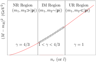
Figure 7: The structure of the Regge trajectory in the $((M-m_{R})^{2},\,x)$ plane where $x=n_{r},\,l$. The behavior in different energy regions accords to Eqs. (34) and (43). The confining potential is assumed to be linear ${\sigma}r$. The circles represent the part of the Regge trajectory in the intermediate region which remains unclear.

Eq. (32) will lead to a generic form of the Regge-like formula which reads Chen:2021kfw

$$(M-m_{R})^{2}=\alpha_{x}(x+c_{0})^{\gamma}\quad(x=l,\,n_{r}),$$ (34)

where

$$m_{R}=m_{1}+m_{2}+\epsilon_{c}.$$ (35)

Eq. (34) is an extension of the Regge-like formulas in Refs. Veseli:1996gy ; Afonin:2014nya ; Afonin:2020bqc ; Chen:2017fcs ; Jia:2019bkr ; Jia:2018yvk ; Chen:2014nyo ; Afonin:2013hla . Using Eqs. (19) and (34), we have for the power-law potentials

$$\left\{\begin{array}[]{cc}\gamma=\frac{4a}{a+2},&\text{NR region},\\ \frac{2a}{a+1}<\gamma<\frac{4a}{a+2},&\text{IM region},\\ \gamma=\frac{2a}{a+1},&\text{UR region}.\end{array}\right.$$ (39)

For the linear confining potential, Eq. (39) becomes

$$\left\{\begin{array}[]{cc}\gamma=\frac{4}{3},&\text{NR region},\\ 1<\gamma<\frac{4}{3},&\text{IM region},\\ \gamma=1,&\text{UR region}.\end{array}\right.$$ (43)

It is shown in Fig. 7.

Eq. (34) can alao be obtained from the new ansatz in Eq. (1), where $m_{R}=c_{1}$, $\alpha_{x}=\beta^{2}_{x}$, $\gamma=2\nu$. In addition, with the help of the Taylor series, the new ansatz $M=\beta_{x}(x+c_{0})^{\nu}+c_{1}$ in Eq. (1) can be approximated as the form of $(M-c_{1})^{2}\approx 2\nu\beta_{x}^{2}c_{0}^{2\nu-1}x+\beta_{x}^{2}c_{0}^{2\nu}$ type Regge trajectory when $\nu\neq 0.5$ if $c_{0}$ is large and the approximation becomes equal when $\nu=0.5$. Similarly, the new ansatz $M=\beta_{x}(x+c_{0})^{\nu}+c_{1}$ can be approximated as the conventional form of Regge trajectory $M^{2}\approx 2\nu\beta_{x}c_{0}^{\nu-1}(\beta_{x}c_{0}^{\nu}+c_{1})x+(\beta_{x}c_{0}^{\nu}+c_{1})^{2}$ ($\nu>0$). If $\beta_{x}(x+c_{0})^{\nu}{\ll}c_{1}$, there is $M^{2}\approx 2c_{1}\beta_{x}(x+c_{0})^{\nu}+c^{2}_{1}$ Chen:2021kfw . If $\beta_{x}(x+c_{0})^{\nu}{\gg}c_{1}$, there is $M^{2}\approx\beta_{x}^{2}(x+c_{0})^{2\nu}$.

The new ansatz in Eq. (1) can be rewritten in a more general form

$$M=\left({\alpha^{\prime}_{l}}\,l+{\alpha^{\prime}_{n_{r}}}n_{r}+c^{\prime}_{0}\right)^{\nu}+c_{1}.$$ (44)

Correspondingly, Eq. (34) has the general form

$$(M-m_{R})^{2}=({\alpha^{\prime}_{l}}\,l+{\alpha^{\prime}_{n_{r}}}n_{r}+c^{\prime}_{0})^{\gamma},$$ (45)

which can be obtained from Eq. (44). When $l\neq 0$ and $n_{r}\neq 0$ simultaneously exist, Eqs. (44) and (45) work evidently. As expected, ${\alpha^{\prime}_{l}}\,l+c^{\prime}_{0}$ in the Regge trajectories increases with $l$ and ${\alpha^{\prime}_{n_{r}}}n_{r}+c^{\prime}_{0}$ increases with $n_{r}$, see Figs. 8, 9 and Table 3.

Appendix B $((M-m_{R})^{2},\,x)$ Regge trajectories for the light nonstrange mesons

In this section, the Regge trajectories for the light nonstrange mesons are fitted individually by the formula in Eq. (34) with $\gamma=1$. The experimental masses are from PDG ParticleDataGroup:2020ssz . The fitted Regge trajectories are listed in Table 3 and shown in Figs. 8, 9. The Regge trajectory formed by $a_{0}(1450)$, $\rho(1700)$ and $\rho_{3}(1990)$ [$M^{2}=0.57\,l+2.70$] and the Regge trajectory formed by $f_{0}(1370)$, $\omega(1650)$ and $f_{2}(1810)$ [$M^{2}=0.74\,l+1.16$] are not listed in Table 3 due to their too small slopes.

As $m_{R}$ increases, $\alpha_{x}$ and $\alpha_{x}{c_{0}}$ will decrease, see Figs. 8, 9 and Table 3. The averaged slope $\overline{\alpha}_{n_{r}}$ for the radial Regge trajectories varies from $1.24$ $\rm{GeV}^{2}$ to $1.14$ $\rm{GeV}^{2}$ and $1.10$ $\rm{GeV}^{2}$ as $m_{R}$ is from $0$ $\rm{GeV}$ to $0.135$ $\rm{GeV}$ and $0.185$ $\rm{GeV}$, see Table 4. The averaged slope $\overline{\alpha}_{l}$ for the orbital Regge trajectories is $1.10$ $\rm{GeV}^{2}$, $1.02$ $\rm{GeV}^{2}$ and $0.98$ $\rm{GeV}^{2}$ for $m_{R}=0$ $\rm{GeV}$, $m_{R}=0.135$ $\rm{GeV}$ and $m_{R}=0.185$ $\rm{GeV}$, respectively.

For the conventional form of the Regge trajectories $M^{2}=\alpha_{l}l+\alpha_{n_{r}}n_{r}+c$, $\alpha_{l}$ is not always equal to $\alpha_{n_{r}}$, see Table 3. If $x\equiv l+{\alpha_{n_{r}}/\alpha_{l}}n_{r}$, the averaged slopes $\overline{\alpha}_{l}$ is not equal to the averaged slopes $\overline{\alpha}_{n_{r}}$ for the light nonstrange mesons, see Table 4. The ratio ${\alpha_{n_{r}}/\alpha_{l}}$ lies in the interval $0.85\leq\alpha_{n_{r}}/\alpha_{l}\leq 1.28$ as $l=n_{r}=0$. As $l=n_{r}=1$, $0.93\leq\alpha_{n_{r}}/\alpha_{l}\leq 1.68$. As $l=n_{r}=2$, $0.95\leq\alpha_{n_{r}}/\alpha_{l}\leq 1.26$. The obtained results are consistent with Refs. Brau:2000st ; Kang:1975cq ; Afonin:2007jd . The effect of $m_{R}$ on the ratio $\alpha_{n_{r}}/\alpha_{l}$ is small as $m_{R}$ ranges from $0$ $\rm{GeV}$ to $0.185$ $\rm{GeV}$.

Table 3: The linearly fitted Regge trajectories for the light nonstrange mesons in the $((M-m_{R})^{2},\,x)$ plane, where $x=n_{r},\,l$.

Traj.		$m_{R}=0$ GeV	$m_{R}=0.135$ GeV	$m_{R}=0.185$ GeV
$\pi^{0}$	$l=0$	1.37 $n_{r}$ + 0.23	1.23 $n_{r}$ + 0.11	1.18 $n_{r}$ + 0.08
$\rho(770)$	$l=0$	1.42 $n_{r}$ + 0.67	1.30 $n_{r}$ + 0.46	1.25 $n_{r}$ + 0.38
$\eta$	$l=0$	1.25 $n_{r}$ + 0.39	1.14 $n_{r}$ + 0.21	1.10 $n_{r}$ + 0.15
$\omega(782)$	$l=0$	1.11 $n_{r}$ + 0.67	1.02 $n_{r}$ + 0.44	0.98 $n_{r}$ + 0.37
$a_{1}(1260)$	$l=1$	1.26 $n_{r}$ + 1.56	1.16 $n_{r}$ + 1.24	1.13 $n_{r}$ + 1.12
$a_{2}(1320)$	$l=1$	1.14 $n_{r}$ + 1.75	1.05 $n_{r}$ + 1.40	1.01 $n_{r}$ + 1.29
$b_{1}(1235)$	$l=1$	1.17 $n_{r}$ + 1.51	1.08 $n_{r}$ + 1.19	1.04 $n_{r}$ + 1.08
$f_{2}(1270)$	$l=1$	1.51 $n_{r}$ + 1.48	1.39 $n_{r}$ + 1.16	1.35 $n_{r}$ + 1.05
$h_{1}(1170)$	$l=1$	1.19 $n_{r}$ + 1.38	1.10 $n_{r}$ + 1.09	1.06 $n_{r}$ + 0.98
$\rho(1700)$	$l=2$	1.09 $n_{r}$ + 2.94	1.01 $n_{r}$ + 2.50	0.99 $n_{r}$ + 2.34
$\pi_{2}(1670)$	$l=2$	1.22 $n_{r}$ + 2.74	1.13 $n_{r}$ + 2.31	1.10 $n_{r}$ + 2.16
$\omega_{3}(1670)$	$l=2$	1.15 $n_{r}$ + 2.73	1.07 $n_{r}$ + 2.30	1.04 $n_{r}$ + 2.15
$\eta_{2}(1645)$	$l=2$	1.22 $n_{r}$ + 2.71	1.13 $n_{r}$ + 2.28	1.10 $n_{r}$ + 2.13
$\pi^{0}/b_{1}$	$n_{r}=0$	1.27 $l$ + 0.16	1.13 $l$ + 0.06	1.08 $l$ + 0.03
$\rho(770)/a_{2}$	$n_{r}=0$	1.12 $l$ + 0.62	1.03 $l$ + 0.39	0.99 $l$ + 0.32
$a_{1}(1260)/\rho_{2}$	$n_{r}=0$	1.13 $l$ + 0.32	1.04 $l$ + 0.09	1.01 $l$ + 0.02
$\eta/h_{1}$	$n_{r}=0$	1.30 $l$ + 0.16	1.18 $l$ + 0.	1.13 $l$ - 0.04
$\omega(782)/f_{2}$	$n_{r}=0$	1.11 $l$ + 0.59	1.02 $l$ + 0.36	0.99 $l$ + 0.29
$\pi(1300)/b_{1}$	$n_{r}=1$	1.11 $l$ + 1.68	1.03 $l$ + 1.34	0.99 $l$ + 1.23
$\rho(1450)/a_{2}$	$n_{r}=1$	0.97 $l$ + 2.06	0.90 $l$ + 1.69	0.87 $l$ + 1.56
$a_{1}(1640)/\rho_{2}$	$n_{r}=1$	1.22 $l$ + 1.46	1.13 $l$ + 1.11	1.10 $l$ + 1.00
$\omega(1420)/f_{2}$	$n_{r}=1$	0.90 $l$ + 1.92	0.83 $l$ + 1.56	0.80 $l$ + 1.44
$\pi(1800)/b_{1}$	$n_{r}=2$	0.97 $l$ + 3.14	0.91 $l$ + 2.68	0.88 $l$ + 2.52
$\eta(1760)/h_{1}$	$n_{r}=2$	0.99 $l$ + 3.00	0.93 $l$ + 2.55	0.90 $l$ + 2.39
$\omega(1650)/f_{2}$	$n_{r}=2$	1.15 $l$ + 3.03	1.07 $l$ + 2.58	1.04 $l$ + 2.42

Table 4: The averaged slopes of the fitted Regge trajectories for the light nonstrange mesons in the $((M-m_{R})^{2},\,x)$ plane, where $x=n_{r},\,l$. The used data are from Table 3. $\overline{\alpha}_{n_{r}}$ and $\overline{\alpha}_{l}$ are in units of $\rm GeV^{2}$.

		$m_{R}=0$ $\rm GeV$	$m_{R}=0.135$ $\rm GeV$	$m_{R}=0.185$ $\rm GeV$
	$l=0$	1.29	1.17	1.13
$\overline{\alpha}_{n_{r}}$	$l=1$	1.25	1.16	1.12
	$l=2$	1.17	1.09	1.07
	$l=0,1,2$	1.24	1.14	1.10
	$n_{r}=0$	1.19	1.08	1.04
$\overline{\alpha}_{l}$	$n_{r}=1$	1.05	0.97	0.94
	$n_{r}=2$	1.04	0.97	0.94
	$n_{r}=0,1,2$	1.10	1.02	0.98

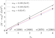
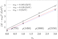
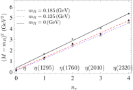
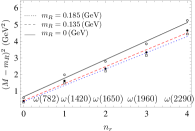
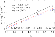
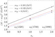
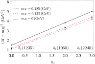
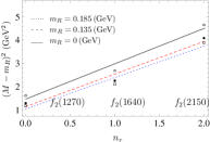
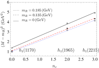
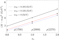
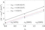
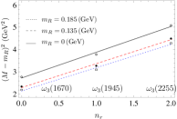
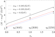
Figure 8: The radial Regge trajectories for the light nonstrange mesons. They are plotted in the $((M-m_{R})^{2},\,n_{r})$ plane. The used formulas are listed in Table 3. The experimental masses are from PDG ParticleDataGroup:2020ssz .

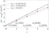
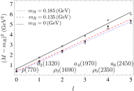
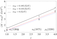
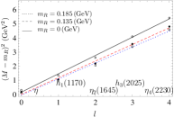
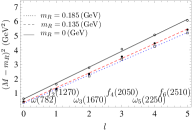
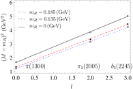
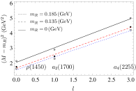
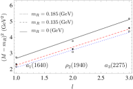
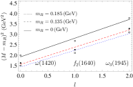
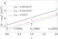
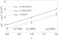
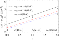
Figure 9: The orbital Regge trajectories for the light nonstrange mesons. They are plotted in the $((M-m_{R})^{2},\,l)$ plane. The used formulas are listed in Table 3. The experimental masses are from PDG ParticleDataGroup:2020ssz .

References

- (1) S. Godfrey and J. Napolitano, Rev. Mod. Phys. 71, 1411-1462 (1999) doi:10.1103/RevModPhys.71.1411 [arXiv:hep-ph/9811410 [hep-ph]].
- (2) T. Regge, Nuovo Cim. 14, 951 (1959).
- (3) P. D. B. Collins, Phys. Rept. 1, 103 (1971); P. D. B. Collins, An Introduction to Regge Theory and High-Energy Physics (Cambridge University Press, London, 1977).
- (4) A. J. G. Hey and R. L. Kelly, Phys. Rept. 96, 71 (1983).
- (5) A. E. Inopin, arXiv: hep-ph/0110160, and references therein.
- (6) H. X. Chen, W. Chen, X. Liu, Y. R. Liu and S. L. Zhu, Rept. Prog. Phys. 80, no. 7, 076201 (2017). arXiv: hep-ph/1609.08928.
- (7) H. X. Chen, W. Chen, X. Liu and S. L. Zhu, Phys. Rept. 639, 1 (2016). arXiv: hep-ph/1601.02092.
- (8) A. Inopin and G. S. Sharov, Phys. Rev. D 63, 054023 (2001). arXiv: hep-ph/9905499.
- (9) G. F. Chew and S. C. Frautschi, Phys. Rev. Lett. 7, 394 (1961).
- (10) G. F. Chew and S. C. Frautschi, Phys. Rev. Lett. 8, 41 (1962).
- (11) S. J. Brodsky, Adv. High Energy Phys. 2018, 7236382 (2018) doi:10.1155/2018/7236382 [arXiv:1709.01191 [hep-ph]].
- (12) The Regge trajectories of hadrons are commenly plotted in the plane or in the plane, where . For simplicity, the figures plotted in the plane Burns:2010qq and in the plane Chen:2017fcs are also called the Regge trajectories.
- (13) A. V. Anisovich, V. V. Anisovich and A. V. Sarantsev, Phys. Rev. D 62, 051502 (2000) doi:10.1103/PhysRevD.62.051502 [arXiv:hep-ph/0003113 [hep-ph]].
- (14) S. S. Afonin, Phys. Lett. B 639, 258-262 (2006) doi:10.1016/j.physletb.2006.06.057 [arXiv:hep-ph/0603166 [hep-ph]].
- (15) M. Shifman and A. Vainshtein, Phys. Rev. D 77, 034002 (2008) doi:10.1103/PhysRevD.77.034002 [arXiv:0710.0863 [hep-ph]].
- (16) D. Ebert, R. N. Faustov and V. O. Galkin, Phys. Rev. D 79 (2009), 114029 doi:10.1103/PhysRevD.79.114029 [arXiv:0903.5183 [hep-ph]].
- (17) P. Masjuan, E. Ruiz Arriola and W. Broniowski, Phys. Rev. D 85, 094006 (2012) doi:10.1103/PhysRevD.85.094006 [arXiv:1203.4782 [hep-ph]].
- (18) I. Y. Kobzarev, B. V. Martemyanov and M. G. Shchepkin, Sov. Phys. Usp. 35, 257-275 (1992) doi:10.1070/PU1992v035n04ABEH002226
- (19) W. Lucha, H. Rupprecht and F. F. Schoberl, Phys. Lett. B 261, 504-509 (1991) doi:10.1016/0370-2693(91)90464-2
- (20) S. S. Afonin and T. D. Solomko, [arXiv:2106.01846 [hep-th]].
- (21) A. Tang and J. W. Norbury, Phys. Rev. D 62, 016006 (2000) doi:10.1103/PhysRevD.62.016006 [arXiv:hep-ph/0004078 [hep-ph]].
- (22) M. M. Brisudova, L. Burakovsky and J. T. Goldman, Phys. Rev. D 61, 054013 (2000) doi:10.1103/PhysRevD.61.054013 [arXiv:hep-ph/9906293 [hep-ph]].
- (23) G. S. Sharov, [arXiv:1305.3985 [hep-ph]].
- (24) J. Sonnenschein and D. Weissman, JHEP 08, 013 (2014) doi:10.1007/JHEP08(2014)013 [arXiv:1402.5603 [hep-ph]].
- (25) J. K. Chen, Eur. Phys. J. A 57, 238 (2021) doi:10.1140/epja/s10050-021-00502-y [arXiv:2102.07993 [hep-ph]].
- (26) J. K. Chen, Eur. Phys. J. C 78, no.3, 235 (2018) doi:10.1140/epjc/s10052-018-5718-z
- (27) J. K. Chen, Phys. Lett. B 786, 477-484 (2018) doi:10.1016/j.physletb.2018.10.022 [arXiv:1807.11003 [hep-ph]].
- (28) J. K. Chen, Eur. Phys. J. C 78, no.8, 648 (2018) doi:10.1140/epjc/s10052-018-6134-0
- (29) M. Kruczenski, L. A. Pando Zayas, J. Sonnenschein and D. Vaman, JHEP 06, 046 (2005) doi:10.1088/1126-6708/2005/06/046 [arXiv:hep-th/0410035 [hep-th]].
- (30) M. A. Martin Contreras and A. Vega, Phys. Rev. D 102 (2020) no.4, 046007 doi:10.1103/PhysRevD.102.046007 [arXiv:2004.10286 [hep-ph]].
- (31) J. Sonnenschein and D. Weissman, Eur. Phys. J. C 79, no.4, 326 (2019) doi:10.1140/epjc/s10052-019-6828-y [arXiv:1812.01619 [hep-ph]].
- (32) M. N. Sergeenko, Z. Phys. C 64, 315-322 (1994) doi:10.1007/BF01557404
- (33) G. Cotugno, R. Faccini, A. D. Polosa and C. Sabelli, Phys. Rev. Lett. 104, 132005 (2010) doi:10.1103/PhysRevLett.104.132005 [arXiv:0911.2178 [hep-ph]].
- (34) T. J. Burns, F. Piccinini, A. D. Polosa and C. Sabelli, Phys. Rev. D 82, 074003 (2010) doi:10.1103/PhysRevD.82.074003 [arXiv:1008.0018 [hep-ph]].
- (35) S. S. Afonin, doi:10.1142/9789811219313_0018 [arXiv:2009.05378 [hep-ph]].
- (36) K. Chen, Y. Dong, X. Liu, Q. F. Lü and T. Matsuki, Eur. Phys. J. C 78, no.1, 20 (2018) doi:10.1140/epjc/s10052-017-5512-3 [arXiv:1709.07196 [hep-ph]].
- (37) D. Jia, W. N. Liu and A. Hosaka, Phys. Rev. D 101, no.3, 034016 (2020) [arXiv:1907.04958 [hep-ph]].
- (38) F. Brau, Phys. Rev. D 62, 014005 (2000) doi:10.1103/PhysRevD.62.014005 [arXiv:hep-ph/0412170 [hep-ph]].
- (39) P. A. Zyla et al. [Particle Data Group], PTEP 2020, no.8, 083C01 (2020) doi:10.1093/ptep/ptaa104
- (40) S. Godfrey and N. Isgur, Phys. Rev. D 32, 189-231 (1985) doi:10.1103/PhysRevD.32.189
- (41) T. Horn and C. D. Roberts, J. Phys. G 43, no.7, 073001 (2016) doi:10.1088/0954-3899/43/7/073001 [arXiv:1602.04016 [nucl-th]].
- (42) E. Eichten, K. Gottfried, T. Kinoshita, J. B. Kogut, K. D. Lane and T. M. Yan, Phys. Rev. Lett. 34, 369-372 (1975) [erratum: Phys. Rev. Lett. 36, 1276 (1976)] doi:10.1103/PhysRevLett.34.369
- (43) D. Flamm, F. Schoberl and H. Umematsu, Nuovo Cim. A 98 (1987), 559 doi:10.1007/BF02902013
- (44) D. B. Lichtenberg, E. Predazzi, R. Roncaglia, M. Rosso and J. G. Wills, Z. Phys. C 41, 615 (1989) doi:10.1007/BF01564705
- (45) K. Heikkila, S. Ono and N. A. Tornqvist, Phys. Rev. D 29, 110 (1984) [erratum: Phys. Rev. D 29, 2136 (1984)] doi:10.1103/PhysRevD.29.2136
- (46) X. Song, J. Phys. G 17, 49 (1991)
- (47) X. t. Song and H. f. Lin, Z. Phys. C 34, 223 (1987) doi:10.1007/BF01566763
- (48) A. Martin, Phys. Lett. B 93, 338-342 (1980) doi:10.1016/0370-2693(80)90527-4
- (49) A. Martin, Phys. Lett. B 100, 511-514 (1981) doi:10.1016/0370-2693(81)90617-1
- (50) A. K. Rai, B. Patel and P. C. Vinodkumar, Phys. Rev. C 78, 055202 (2008) doi:10.1103/PhysRevC.78.055202 [arXiv:0810.1832 [hep-ph]].
- (51) B. Patel and P. C. Vinodkumar, J. Phys. G 36, 035003 (2009) doi:10.1088/0954-3899/36/3/035003 [arXiv:0808.2888 [hep-ph]].
- (52) A. H. Fariborz and M. Lyukova, [arXiv:2107.12266 [hep-ph]].
- (53) J. Arrington, C. A. Gayoso, P. C. Barry, V. Berdnikov, D. Binosi, L. Chang, M. Diefenthaler, M. Ding, R. Ent and T. Frederico, et al. J. Phys. G 48, no.7, 075106 (2021) doi:10.1088/1361-6471/abf5c3 [arXiv:2102.11788 [nucl-ex]].
- (54) C. Alexandrou, J. Berlin, M. Dalla Brida, J. Finkenrath, T. Leontiou and M. Wagner, Phys. Rev. D 97 (2018) no.3, 034506 doi:10.1103/PhysRevD.97.034506 [arXiv:1711.09815 [hep-lat]].
- (55) N. Santowsky and C. S. Fischer, [arXiv:2109.00755 [hep-ph]].
- (56) R. Frezzotti, G. Gagliardi, V. Lubicz, G. Martinelli, F. Sanfilippo and S. Simula, [arXiv:2202.11970 [hep-lat]].
- (57) M. Baldicchi, A. V. Nesterenko, G. M. Prosperi, D. V. Shirkov and C. Simolo, Phys. Rev. Lett. 99 (2007), 242001 doi:10.1103/PhysRevLett.99.242001 [arXiv:0705.0329 [hep-ph]].
- (58) M. Baldicchi, A. V. Nesterenko, G. M. Prosperi and C. Simolo, Phys. Rev. D 77 (2008), 034013 doi:10.1103/PhysRevD.77.034013 [arXiv:0705.1695 [hep-ph]].
- (59) N. Brambilla, E. Montaldi and G. M. Prosperi, Phys. Rev. D 54 (1996), 3506-3525 doi:10.1103/PhysRevD.54.3506 [arXiv:hep-ph/9504229 [hep-ph]].
- (60) J. K. Chen, Acta Phys. Pol. B 47, 1155 (2016)
- (61) J. K. Chen, Rom. J. Phys. 62, 119 (2017)
- (62) B. Durand and L. Durand, Phys. Rev. D 25, 2312 (1982) doi:10.1103/PhysRevD.25.2312
- (63) B. Durand and L. Durand, Phys. Rev. D 30, 1904 (1984) doi:10.1103/PhysRevD.30.1904
- (64) D. B. Lichtenberg, W. Namgung, E. Predazzi and J. G. Wills, Phys. Rev. Lett. 48, 1653 (1982) doi:10.1103/PhysRevLett.48.1653
- (65) S. Jacobs, M. G. Olsson and C. Suchyta, III, Phys. Rev. D 33, 3338 (1986) [erratum: Phys. Rev. D 34, 3536 (1986)] doi:10.1103/PhysRevD.33.3338
- (66) D. Gromes, Z. Phys. C 11, 147 (1981) doi:10.1007/BF01573997
- (67) W. Lucha, F. F. Schoberl and D. Gromes, Phys. Rept. 200, 127-240 (1991) doi:10.1016/0370-1573(91)90001-3
- (68) S. Tomonaga, Quantum Mechanics, Volume I: Old Quantum Theory (North-Holland Publishing Company, Amsterdam, 1962)
- (69) A. Martin, Z. Phys. C 32, 359 (1986) doi:10.1007/BF01551832
- (70) M. Fabre De La Ripelle, Phys. Lett. B 205 (1988), 97-102 doi:10.1016/0370-2693(88)90406-6
- (71) C. Quigg and J. L. Rosner, Phys. Rept. 56 (1979), 167-235 doi:10.1016/0370-1573(79)90095-4
- (72) R. L. Hall, Phys. Rev. D 30 (1984), 433-436 doi:10.1103/PhysRevD.30.433
- (73) M. G. Olsson, S. Veseli and K. Williams, Phys. Rev. D 51, 5079-5089 (1995) doi:10.1103/PhysRevD.51.5079 [arXiv:hep-ph/9410405 [hep-ph]].
- (74) J. S. Kang and H. J. Schnitzer, Phys. Rev. D 12, 841 (1975) doi:10.1103/PhysRevD.12.841
- (75) L. K. Sharma and V. P. Iyer, J. Math. Phys. 23, 1185-1189 (1982) doi:10.1063/1.525450
- (76) D. A. Kulikov and R. S. Tutik, [arXiv:hep-ph/0608260 [hep-ph]].
- (77) D. E. Kahana, K. M. Maung and J. W. Norbury, Phys. Rev. D 48, 3408-3409 (1993) doi:10.1103/PhysRevD.48.3408
- (78) M. Baldicchi and G. M. Prosperi, Phys. Lett. B 436, 145-152 (1998) doi:10.1016/S0370-2693(98)00830-2 [arXiv:hep-ph/9803390 [hep-ph]].
- (79) M. Baldicchi, [arXiv:hep-ph/9911268 [hep-ph]].
- (80) E. Di Salvo, L. Kondratyuk and P. Saracco, Z. Phys. C 69, 149-162 (1995) doi:10.1007/s002880050015 [arXiv:hep-ph/9411309 [hep-ph]].
- (81) A. Selem and F. Wilczek, doi:10.1142/9789812773524_0030 [arXiv:hep-ph/0602128 [hep-ph]].
- (82) Y. Nambu, Phys. Rev. D 10, 4262 (1974) doi:10.1103/PhysRevD.10.4262
- (83) S. S. Afonin and I. V. Pusenkov, Phys. Rev. D 90, no.9, 094020 (2014) doi:10.1103/PhysRevD.90.094020 [arXiv:1411.2390 [hep-ph]].
- (84) A. Karch, E. Katz, D. T. Son and M. A. Stephanov, Phys. Rev. D 74 (2006), 015005 doi:10.1103/PhysRevD.74.015005 [arXiv:hep-ph/0602229 [hep-ph]].
- (85) S. J. Brodsky, G. F. de Téramond, H. G. Dosch and C. Lorcé, Phys. Lett. B 759 (2016), 171-177 doi:10.1016/j.physletb.2016.05.068 [arXiv:1604.06746 [hep-ph]].
- (86) E. Folco Capossoli, M. A. Martín Contreras, D. Li, A. Vega and H. Boschi-Filho, Chin. Phys. C 44, no.6, 064104 (2020) doi:10.1088/1674-1137/44/6/064104 [arXiv:1903.06269 [hep-ph]].
- (87) S. Veseli and M. G. Olsson, Phys. Lett. B 383, 109-115 (1996) doi:10.1016/0370-2693(96)00721-6 [arXiv:hep-ph/9606257 [hep-ph]].
- (88) D. J. Jia and W. C. Dong, [arXiv:1804.08112 [hep-ph]].
- (89) S. S. Afonin and I. V. Pusenkov, Mod. Phys. Lett. A 29, no.35, 1450193 (2014) doi:10.1142/S0217732314501934 [arXiv:1308.6540 [hep-ph]].
- (90) B. Chen, K. W. Wei and A. Zhang, Eur. Phys. J. A 51, 82 (2015) doi:10.1140/epja/i2015-15082-3 [arXiv:1406.6561 [hep-ph]].
- (91) S. S. Afonin, Mod. Phys. Lett. A 22, 1359-1372 (2007) doi:10.1142/S0217732307024024 [arXiv:hep-ph/0701089 [hep-ph]].