Random walks on crystal lattices and multiple zeta functions

Abstract.

Crystal lattices are known to be one of the generalizations of classical periodic lattices which can be embedded into some Euclidean spaces properly. As to make a wide range of multidimensional discrete distributions on Euclidean spaces more treatable, multidimensional Euler products and multidimensional Shintani zeta functions on crystal lattices are introduced. They are completely different from existing Ihara zeta functions on graphs in that our zeta functions are defined on crystal lattices directly. Via a concept of periodic realizations of crystal lattices, we make it possible to provide many kinds of multidimensional discrete distributions explicitly. In particular, random walks on crystal lattices whose range is infinite and such random walks whose range is finite are constructed by multidimensional Euler products and multidimensional Shintani zeta functions, respectively. We give some comprehensible examples as well.

1. Introduction

1.1. Riemann zeta functions in probabilistic view

Zeta functions have been investigated extensively in number theory and other areas among mathematics. The most classical one is known as the Riemann zeta function $\zeta(s)$. It is a function of a complex variable $s=\sigma+\mathrm{i}t$ for $\sigma>1$ and $t\in\mathbb{R}$ given by

$$\zeta(s):=\sum_{n=1}^{\infty}\frac{1}{n^{s}}=\prod_{p\in\mathbb{P}}\Big{(}1-\frac{1}{p^{s}}\Big{)}^{-1},$$ (1.1)

where we denote by $\mathbb{P}$ the set of all prime numbers. The product representation of (1.1) is called the Euler product. It is known that the function $\zeta(s)$ converges absolutely in the half-plane $\{\sigma+\mathrm{i}t\,|\,\sigma>1\}$ and uniformly in every compact subset of the half-plane. We also note that the Riemann zeta function can be extended to a meromorphic function on the complex plane $\mathbb{C}$ having a single pole at $s=1$ by analytic continuation.

On the other hand, there exists a well-known relation between the Riemann zeta function $\zeta(s)$ and probability distributions on $\mathbb{R}$. We refer to [JW35], [Khi38], [GK68] and [LH01]. Afterwards, Biane, Pitman and Yor [BPY01] reviewed some known results on the Riemann zeta function in probabilistic view. See also [BHNY08] for an interesting topic among the Riemann zeta function, Jacobi theta function and some probability distributions.

Before we state the relation, we review a terminology in probability theory.

Definition 1.1 (infinite divisible distribution).

A probability measure $\mu$ on $\mathbb{R}^{d}$ is said to be infinitely divisible if, for any positive integer $n$, there exists a probability measure $\mu_{n}$ on $\mathbb{R}^{d}$ such that $\mu=\mu_{n}^{*n}$, where $\mu_{n}^{*n}$ is the $n$-fold convolution of $\mu_{n}$ itself.

We denote by $I(\mathbb{R}^{d})$ the set of all infinitely divisible probability measures on $\mathbb{R}^{d}$. Let $\mu$ be a probability measure on $\mathbb{R}^{d}$ and

$$\widehat{\mu}(\vec{t}):=\int_{\mathbb{R}^{d}}\mathrm{e}^{\mathrm{i}\langle\vec{t},\vec{x}\rangle}\,\mu(d\vec{x}),\qquad\vec{t}\in\mathbb{R}^{d},$$

the characteristic function of $\mu$, where $\langle\cdot,\cdot\rangle$ is the usual inner product on $\mathbb{R}^{d}$. It is easily seen that $\mu\in I(\mathbb{R}^{d})$ if and only if the $n$-th root of its characteristic function $\widehat{\mu}^{1/n}$ is also a characteristic function for every $n\in\mathbb{N}$. Note that this class is important when we consider probabilistic limit theorems given by sums of independent and identically distributed random variables such as the central limit theorem and the law of large numbers.

Example 1.2 (compound Poisson distribution).

The class of compound Poisson distributions is known as one of the most important subclasses of infinitely divisible distributions. A probability distribution $\mu_{\mathrm{CP}}$ is compound Poisson if its characteristic function is given by

$$\widehat{\mu_{\mathrm{CP}}}(\vec{t})=\exp\Big{(}\lambda\big{(}\widehat{\rho}(\vec{t})-1\big{)}\Big{)},\qquad\vec{t}\in\mathbb{R}^{d},$$

for some $\lambda>0$ and some distribution $\rho$ with $\rho(\{0\})=0$. Note that the Poisson distribution is a special case when $d=1$ and $\rho=\delta_{1}$, where $\delta_{1}$ is the delta measure at $x=1$.

Let $Y$ be an $\mathbb{R}^{d}$-valued random variable whose distribution is $\rho$. We take independent copies $Y_{1},Y_{2},\dots$ of $Y$ and a Poisson random variable $K$ with a parameter $\lambda>0$ independent of $Y$. Then the characteristic function $\widehat{\mu_{Z}}$ of a random variable $Z:=Y_{1}+Y_{2}+\cdots+Y_{K}$ is given by

$$\widehat{\mu_{Z}}(\vec{t}) =\mathbf{E}\big{[}\mathrm{e}^{\mathrm{i}\langle\vec{t},Y_{1}+Y_{2}+\cdots+Y_{K}\rangle}\big{]}=\sum_{n=1}^{\infty}\mathbf{E}\big{[}\mathrm{e}^{\mathrm{i}\langle\vec{t},Y_{1}+Y_{2}+\cdots+Y_{n}\rangle}:K=n\big{]}$$

$$=\sum_{n=1}^{\infty}\widehat{\rho}(\vec{t})^{n}\cdot\Big{(}\mathrm{e}^{-\lambda}\frac{\lambda^{n}}{n!}\Big{)}=\exp\Big{(}\lambda\big{(}\widehat{\rho}(\vec{t})-1\big{)}\Big{)},\qquad\vec{t}\in\mathbb{R}^{d},$$

which means that the distribution of $Z$ is of compound Poisson.

The following is well-known.

Proposition 1.3 (Lévy–Khintchine representation, cf. [Sat99, Theorem 8.1]).

(1) If $\mu\in I(\mathbb{R}^{d})$, then we have

$$\widehat{\mu}(\vec{t})=\exp\Big{(}-\frac{1}{2}\langle A\vec{t},\vec{t}\rangle+\mathrm{i}\langle\vec{\gamma},\vec{t}\rangle+\int_{\mathbb{R}^{d}}\Big{(}\mathrm{e}^{\mathrm{i}\langle\vec{t},\vec{x}\rangle}-1-\frac{\mathrm{i}\langle\vec{t},\vec{x}\rangle}{1+|\vec{x}|^{2}}\Big{)}\,\nu(d\vec{x})\Big{)},\quad\vec{t}\in\mathbb{R}^{d},$$ (1.2)

where $A$ is a symmetric non-negative definite $d\times d$-matrix, $\nu$ is a measure on $\mathbb{R}^{d}$ satisfying

$$\nu(\{0\})=0\quad\text{and}\quad\int_{\mathbb{R}^{d}}\min\{|\vec{x}|^{2},1\}\,\nu(d\vec{x})<+\infty$$ (1.3)

and $\vec{\gamma}\in\mathbb{R}^{d}$.

(2) The representation of $\widehat{\mu}$ in (1.2) by $A$, $\nu$ and $\vec{\gamma}$ is unique.

(3) Conversely, if $A$ is a symmetric non-negative definite $d\times d$-matrix, $\nu$ is a measure on $\mathbb{R}^{d}$ satisfying (1.3) and $\vec{\gamma}\in\mathbb{R}^{d}$, then there exists $\mu\in I(\mathbb{R}^{d})$ whose characteristic function is given by (1.2).

The measure $\nu$ and the triplet $(A,\nu,\vec{\gamma})$ are called a Lévy measure and a Lévy–Khintchine triplet of $\mu\in I(\mathbb{R}^{d})$, respectively. There is another form of (1.2) if the Lévy measure $\nu$ satisfies an additional condition.

Proposition 1.4 (cf. [Sat99, Section 8]).

In Proposition 1.3, if the Lévy measure $\nu$ in (1.2) satisfies $\int_{|\vec{x}|<1}|\vec{x}|\,\nu(d\vec{x})<+\infty$, then we can rewrite the representation (1.2) by

$$\widehat{\mu}(\vec{t})=\exp\Big{(}-\frac{1}{2}\langle A\vec{t},\vec{t}\rangle+\mathrm{i}\langle\vec{\gamma}_{0},\vec{t}\rangle+\int_{\mathbb{R}^{d}}\big{(}\mathrm{e}^{\mathrm{i}\langle\vec{t},\vec{x}\rangle}-1\big{)}\,\nu(d\vec{x})\Big{)},\qquad\vec{t}\in\mathbb{R}^{d},$$ (1.4)

where $\vec{\gamma}_{0}:=\vec{\gamma}-\int_{|\vec{x}|<1}\vec{x}(1+|\vec{x}|^{2})^{-1}\,\nu(d\vec{x})$.

Let us go back to the Riemann zeta function $\zeta(s)$. Next we introduce a class of probability distributions on $\mathbb{R}$ generated by $\zeta(s)$.

Definition 1.5 (Riemann zeta distribution on $\mathbb{R}$, cf. [GK68]).

Fix $\sigma>1$. A probability distibution $\mu_{\sigma}$ is called a Riemann zeta distribution if

$$\mu_{\sigma}(\{-\log n\})=\frac{n^{-\sigma}}{\zeta(\sigma)},\qquad n\in\mathbb{N}.$$ (1.5)

It is readily verified that the function given by

$$f_{\sigma}(t):=\frac{\zeta(\sigma+\mathrm{i}t)}{\zeta(\sigma)},\qquad t\in\mathbb{R},$$

coincides with the characteristic function of $\mu_{\sigma}$ (see e.g., [GK68]). Moreover, the Riemann zeta distribution is known to be infinitely divisible.

Proposition 1.6 (cf. [GK68]).

Let $\mu_{\sigma}$ be a Riemann zeta distribution on $\mathbb{R}$. Then, $\mu_{\sigma}$ is of compound Poisson on $\mathbb{R}$ and

$$\log f_{\sigma}(t)=\sum_{p\in\mathbb{P}}\sum_{r=1}^{\infty}\frac{p^{-r\sigma}}{r}\left(\mathrm{e}^{-{\rm i}rt\log p}-1\right)=\int_{0}^{\infty}\left(\mathrm{e}^{-{\rm i}tx}-1\right)N_{\sigma}(dx),\qquad t\in\mathbb{R},$$ (1.6)

where $N_{\sigma}$ is a finite Lévy measure on $\mathbb{R}$ given by

$$N_{\sigma}(dx)=\sum_{p\in\mathbb{P}}\sum_{r=1}^{\infty}\frac{p^{-r\sigma}}{r}\delta_{r\log p}(dx).$$

We can also explain Equation (1.6) in terms of random variables. Fix $\sigma>1$. We define an $\mathbb{R}$-valued random variable $Y_{\sigma}$ given by

$$\mathbf{P}(Y_{\sigma}=-r\log p)=\frac{1}{N_{\sigma}(\mathbb{R})}\cdot\frac{p^{-r\sigma}}{r},\qquad r\in\mathbb{N},\,p\in\mathbb{P}.$$

Let $Y_{\sigma}^{1},Y_{\sigma}^{2},\dots$ be independent copies of $Y_{\sigma}$ and $K_{\sigma}$ be a Poisson random variable with a parameter $N_{\sigma}(\mathbb{R})>0$ independent of $Y_{\sigma}$. Then we see that the probability distribution of a random variable $Z_{\sigma}:=Y_{\sigma}^{1}+Y_{\sigma}^{2}+\cdots+Y_{\sigma}^{K_{\sigma}}$ coincides with $\mu_{\sigma}$ given by (1.5).

1.2. Multidimensional zeta functions in probabilistic view

As mentioned in the previous subsection, the Riemann zeta distribution is one of the examples of discrete probability distributions on $\mathbb{R}$ with infinitely many mass points. However, only a few examples of such discrete probability distributions are known explicitly when we look at higher dimension cases. In order to treat such discrete distributions extensively, multidimensional Shintani zeta functions are introduced in view of series representations and investigated some useful relations with probability theory in [AN13b].

For $\vec{c}\in\mathbb{R}^{d}$ and $\vec{s}\in\mathbb{C}^{d}$, we write $\langle\vec{c},\vec{s}\rangle:=\langle\vec{c},\vec{\sigma}\rangle+{\rm i}\langle\vec{c},\vec{t}\rangle$, where $\vec{\sigma},\vec{t}\in\mathbb{R}^{d}$ and $\vec{s}=\vec{\sigma}+{\rm i}\vec{t}$.

Definition 1.7 (multidimensional Shintani zeta function, cf. [AN13b]).

Let $d,m,r\in\mathbb{N}$, $\vec{s}\in\mathbb{C}^{d}$ and $(n_{1},n_{2},\dots,n_{r})\in\mathbb{Z}_{\geq 0}^{r}$. For $\lambda_{\ell j},u_{j}>0$, $\vec{c}_{\ell}\in\mathbb{R}^{d}$, where $j=1,2,\dots,r$ and $\ell=1,2,\dots,m$, and a $\mathbb{C}$-valued function $\theta(n_{1},n_{2},\dots,n_{r})$ satisfying $|\theta(n_{1},n_{2},\dots,n_{r})|=O\big{(}(n_{1}+n_{2}+\cdots+n_{r})^{\varepsilon}\big{)}$, for any $\varepsilon>0$, we define a multidimensional Shintani zeta function $Z_{S}(\vec{s})$ by

$$Z_{S}(\vec{s}):=\sum_{n_{1},n_{2},\dots,n_{r}=0}^{\infty}\frac{\theta(n_{1},n_{2},\dots,n_{r})}{\prod_{\ell=1}^{m}\big{(}\sum_{j=1}^{r}\lambda_{\ell j}(n_{j}+u_{j})\big{)}^{\langle\vec{c}_{\ell},\vec{s}\rangle}}.$$ (1.7)

We write $\mathcal{Z}_{S}^{(d)}$ for the class consisting of all $d$-dimensional Shintani zeta functions of the form (1.7). Put $\vec{s}:=\vec{\sigma}+{\rm i}\vec{t},\,\vec{\sigma},\vec{t}\in\mathbb{R}^{d}.$ The absolute convergence of $Z_{S}(\vec{s})$ is given as follows:

Proposition 1.8 (cf. [AN13b, Theorem 1]).

The series defined by $\eqref{Shintani zeta}$ converges absolutely in the region $\min\{\mathrm{Re}\,\langle\vec{c}_{\ell},\vec{s}\rangle|\,\ell=1,2,\dots m\}>r/m$.

Let $\theta(n_{1},n_{2},\dots,n_{r}),\,(n_{1},n_{2},\dots,n_{r})\in\mathbb{Z}^{r}_{\geq 0}$, be a nonnegative or nonpositive definite function and $\vec{\sigma}\in\mathbb{R}^{d}$ a vector satisfying $\min\{\mathrm{Re}\,\langle\vec{c}_{\ell},\vec{\sigma}\rangle|\,\ell=1,2,\dots,m\}>r/m$. Then, as an extension of the Riemann zeta case, it is shown in [AN13b, Theorem 3] that Shintani zeta functions also generate characteristic functions of probability distributions on $\mathbb{R}^{h},1\leq h\leq d,$ by putting

$$f_{\vec{\sigma}}(\vec{t}):=\frac{Z_{S}(\vec{\sigma}+\mathrm{i}\vec{t})}{Z_{S}(\vec{\sigma})},\qquad\vec{t}\in\mathbb{R}^{d}.$$

However, there exists no effective methods to know their infinite divisibilities. As to show that, they introduced a new multidimensional polynomial Euler products in [AN13c]

Definition 1.9 (multidimensional polynomial Euler product, cf. [AN13c]).

Let $d,\,m\in\mathbb{N}$ and $\vec{s}\in\mathbb{C}^{d}$. For $-1\leq\alpha_{\ell}(p)\leq 1$ and $\vec{a}_{\ell}\in\mathbb{R}^{d}$, $\ell=1,2,\dots,m$ and $p\in\mathbb{P}$, we define a $d$-dimensional polynomial Euler product $Z_{E}(\vec{s})$ given by

$$Z_{E}(\vec{s}):=\prod_{p\in\mathbb{P}}\prod_{\ell=1}^{m}\big{(}1-\alpha_{\ell}(p)p^{-\langle\vec{a}_{\ell},\vec{s}\rangle}\big{)}^{-1}.$$ (1.8)

We write $\mathcal{Z}_{E}^{(d)}$ for the class consisting of all $d$-dimensional polynomial Euler product of the form (1.8). Note that the multidimensional polynomial Euler products were generalized to complex coefficients cases in [Nak16]. We can see that the product (1.8) also converges absolutely.

Proposition 1.10 (cf. [AN13c, Theorem 2.3]).

$Z_{E}(\vec{s})$ converges absolutely and has no zeros in the region $\min\{\mathrm{Re}\,\langle\vec{a}_{\ell},\vec{s}\rangle|\,\ell=1,2,\dots,m\}>1$.

Let $\vec{\sigma}\in\mathbb{R}^{d}$ be a vector satisfying $\min\{\mathrm{Re}\,\langle\vec{a}_{\ell},\vec{\sigma}\rangle|\,\ell=1,2,\dots,m\}>1$. We now put

$$f_{\vec{\sigma}}(\vec{t}):=\frac{Z_{E}(\vec{\sigma}+\mathrm{i}\vec{t})}{Z_{E}(\vec{\sigma})},\qquad\vec{t}\in\mathbb{R}^{d}.$$

Then we may expect that the function $f_{\vec{\sigma}}(\vec{t})$ is also to be a characteristic function as well as the case of Shintani zeta functions. However, it is not trivial that $f_{\vec{\sigma}}(\vec{t})$ to be a characteristic function of some probability distribution on $\mathbb{R}^{d}$. Therefore, it is natural to ask when $f_{\vec{\sigma}}(\vec{t})$ to be so. To find that out, the following two conditions for $\mathbb{R}^{d}$-valued vectors $\vec{a}_{\ell},\,\ell=1,2,\dots,m$, were introduced in [AN13c].

• $\vec{a}_{\ell},\,\ell=1,2,\dots,m$, are linearly independent.

• $\vec{a}_{\ell},\,\ell=1,2,\dots,m$, are linearly dependent but linearly independent over the rationals. Namely, for some $\vec{a}\in\mathbb{R}^{d}$, it holds that $\vec{a}_{\ell}=\psi_{\ell}\vec{a},\,\ell=1,2,\dots,m$, where each $\psi_{\ell}$ are algebraic real numbers and linearly independent over the rationals.

Under either of these two conditions, a necessary and sufficient condition for $f_{\vec{\sigma}}$ to be a characteristic function was obtained as in the following.

Proposition 1.11 (cf. [AN13c, Theorem 3.8]).

Suppose that $\vec{a}_{\ell},\,\ell=1,2,\dots,m$, in (1.8) satisfy either (LI) or (LR). Then $f_{\vec{\sigma}}(\vec{t})$ is a characteristic function if and only if $\alpha_{\ell}(p)\geq 0$ for all $\ell=1,2,\dots,m$ and $p\in\mathbb{P}$. Moreover, $f_{\vec{\sigma}}(\vec{t})$ is a compound Poisson characteristic function with its finite Lévy measure $N_{\vec{\sigma}}(d\vec{x})$ on $\mathbb{R}^{d}$ given by

$$N_{\vec{\sigma}}(d\vec{x})=\sum_{p\in\mathbb{P}}\sum_{r=1}^{\infty}\sum_{\ell=1}^{m}\frac{1}{r}\alpha_{\ell}(p)^{r}p^{-r\langle\vec{a}_{\ell},\vec{\sigma}\rangle}\delta_{(r\log p)\vec{a}_{\ell}}(d\vec{x}).$$

1.3. The purpose of the paper

Random walks on graphs are one of the first contacts in graph theory and probability theory. We often regard some good, periodic and so on, graphs as crystal lattices in Euclidean space by a transformation called a realization. By adopting simple random walks, which are allowed to move to one of the nearest neighbors at each steps, we have rich mathematical observations among geometry and graph theory. Some probabilistic limit theorems such as the central limit theorem and the large deviation principle are shown in some cases and they let us know how nice, symmetric and so on, the graphs are. See e.g., [Sun13] and [Woe00] for details of such developments with extensive references therein.

Though simple random walks are good enough for us to study comprehensive graphs, we need more general random walks to understand properties of complicated ones. There were some difficulties to do such things for the lack of existences of treatable multivariate functions which are the Fourier transformations (i.e., characteristic functions) of multidimensional discrete distributions with finite and especially infinite supports. To break the walls, Aoyama and Nakamura have introduced some new multiple series and infinite products which are called multidimensional Shintani zeta functions and multidimensional polynomial Euler products as mentioned above, respectively. They made it useful for us to describe some linearly or periodically supported discrete distributions in Euclidean spaces by applying analytic number theory. In the present paper, we try to give a new contact of graphs and general random walks by using their multiple zeta functions to break some walls left.

Here, we should mention that there are some existing studies on zeta functions on graphs. The study of zeta functions on graphs dates back to 1960s. It was originated in [Iha66] considering a $p$-adic analogue of Selberg zeta functions, which are now called Ihara zeta functions. The Ihara zeta function is defined by a kind of the Euler product on the set of so-called “prime cycles” in finite graphs. See e.g., [KS00b] for the definition and some properties of the function. It is known that there are explicit relations with the Riemann and some generalized zeta functions appeared in number theory. Several interesting aspects of the Ihara zeta function related to e.g. spectral geometry on finite graphs and random matrix theory with extensive references can be found in [Ter10]. Some authors have considered extensions of Ihara zeta functions to some infinite graph cases by applying operator-algebraic approaches. See e.g., [GIL08] and [LPS19] for more details and references therein.

On the other hand, we here emphasize that such Ihara zeta functions may not be useful when we try to capture probabilistic objects such as random walks and even treatable probability distributions on infinite graphs. In fact, it is difficult to capture random trajectories on graphs via the Ihara zeta function, since each factor of the function is given in terms of a certain coset of “cycles” in the graphs. Furthermore, the study of Ihara zeta functions has been developed mainly in the context of geometry of graphs. On the contrary, the multiple zeta functions introduced in the present paper are completely different from Ihara zeta functions. In view of some known observations among classical zeta functions and probabilistic objects, we believe that more fruitful contributions to random walks on graphs can be obtained by making use of such multiple zeta functions.

The rest of the present paper is organized as follows: We review some basic terminologies from graph theory and introduce notions of crystal lattices and their periodic realizations into some Euclidean spaces in Section 2. We introduce multidimensional Shintani zeta functions on crystal lattices in Section 3. We see that some finite range random walks on crystal lattices are defined in terms of the multidimensional Shintani zeta functions. As a counterpart of Section 3, we consider multidimensional polynomial Euler products on crystal lattices and study a certain subclass of them in Section 4. We also see that some infinite range random walks on crystal lattices are defined in terms of the multidimensional “finite” Euler products. Several comprehensible examples of crystal lattices of dimension 1 and 2 and multiple zeta functions on them are given as well in Section 5.

2. Crystal lattices and their periodic realizations

2.1. Covering graphs

There exist a lot of classes of infinite graphs which possess geometric features such as periodicities, volume growths and so on. Crystal lattices are known as one of the most typical classes of periodic graphs and have been well-studied from geometric perspectives. Such graphs are regarded as discrete analogues of covering spaces of compact manifolds. In particular, their periodicities are clearly described in terms of covering transformation groups. For more details, we refer to [KS06] and [Sun13].

Let $X=(V,E)$ be an oriented and connected graph, where $V$ is the set of all vertices and $E$ is the set of all oriented edges. For an oriented edge $e\in E$, we denote by $o(e)$ and $t(e)$ the origin and the terminus of $e$, respectively. The inverse edge of $e\in E$ is an edge $\overline{e}\in E$ satisfying $o(\overline{e})=t(e)$ and $t(\overline{e})=o(e)$. Note that our graphs possibly have loops ($e\in E$ with $o(e)=t(e)$) and multiple edges ($e_{1},e_{2}\in E$ with $e_{1}\neq e_{2}$, $o(e_{1})=o(e_{2})$ and $t(e_{1})=t(e_{2})$). A path $c$ in $X$ of length $n$ is a sequence $c=(e_{1},e_{2},\dots,e_{n})$ of $n$ edges $e_{1},e_{2},\dots,e_{n}\in E$ with $o(e_{i+1})=t(e_{i})$ for $i=1,2,\dots,n-1$. We denote by $\Omega_{x,n}(X)$ the set of all paths in $X$ of length $n\in\mathbb{N}\cup\{\infty\}$ starting from $x\in V$.

We write $E_{x}$ for the set of all edges whose origin is $x\in V$, that is,

$$E_{x}=\{e\in E\,|\,o(e)=x\},\qquad x\in V.$$

Throughout the present paper, we always consider locally finite graph, that is, $\deg(x):=|E_{x}|<\infty$ for $x\in V.$

The group of all automorphisms on a set $M$ is denoted by $\mathrm{Aut}(M)$. The notion of group actions on graphs is stated as in the following.

Definition 2.1 (group action).

(1) We say that a group $G$ acts on a graph $X=(V,E)$ if two homomorphisms $\phi_{V}:G\to\mathrm{Aut}(V)$ and $\phi_{E}:G\to\mathrm{Aut}(E)$ are given and they satisfy that

$$o\big{(}\phi_{E}(g)e\big{)}=\phi_{V}(g)o(e),\qquad t\big{(}\phi_{E}(g)e\big{)}=\phi_{V}(g)t(e)$$

and there is no edges with $\phi_{E}(g)e=\overline{e}$ for $g\in G$. We denote the actions of $g\in G$ on $x\in V$ and $e\in E$ by $gx$ and $ge$, respectively.

(2) We say that a group $G$ acts on $X$ freely if $gx=hx$ implies $g=h$ for every $x\in V$.

Let $X=(V,E)$ be a graph and suppose that a group $G$ acts on $X$ freely. We put $V_{0}:=G\backslash V$ and $E_{0}:=G\backslash E$, the orbits for the $G$-action. Then we can find a unique graph structure $X_{0}:=(V_{0},E_{0})$ with a canonical projections $\pi_{V}:V\to V_{0}$ and $\pi_{E}:E\to E_{0}$. The graph $X_{0}$ is called a quotient graph of $X$ by the $G$-action and it is denoted by $G\backslash X$.

We here introduce the notion of covering graphs as a geometric analogue of Galois theory in abstract algebra. Let $X_{0}=(V_{0},E_{0})$ be a connected and finite graph. Then the concept of covering map is defined as follows:

Definition 2.2 (covering map and covering graph).

A morphism $\pi:X\to X_{0}$ is said to be a covering map if $\pi:V\to V_{0}$ is surjective and the restriction map $\pi|_{E_{x}}:E_{x}\to(E_{0})_{\pi(x)}$ is bijective for every $x\in V$. We call $X$ a covering graph of $X_{0}$.

Namely, the covering map $\pi$ preserves the information of local relations between vertices and edges. The following is the definition of covering transformation group corresponding to covering graphs.

Definition 2.3 (covering transformation group).

Let $X$ be a covering graph of a finite graph $X_{0}$ and $\pi:X\to X_{0}$ a covering map. An automorphism $\gamma$ of $X$ is called a covering transformation if $\pi\circ\gamma=\gamma$. The set of all covering transformations of $X$ forms a group $\Gamma$ under the composition of maps, which is called a covering transformation group of $X$.

It is easily seen that the covering transformation group $\Gamma$ acts on the graph $X$ freely. Namely, if there is a vertex $x\in V$ satisfying $\gamma x=x$, then $\gamma=\bm{1}_{\Gamma}$ follows, where $\bm{1}_{\Gamma}$ stands for the unit of $\Gamma$. Moreover, we assume that the covering map $\pi:X\to X_{0}$ is regular throughout the present paper, that is, the free action of $\Gamma$ on every fiber $\pi^{-1}(x),\,x\in V,$ is transitive. We then know that the quotient graph $\Gamma\backslash X$ is isomorphic to $X_{0}$, so that the canonical surjection $\pi:X\to\Gamma\backslash X$ is a regular covering map whose covering transformation group is $\Gamma$.

Our focus of interest is the following.

Definition 2.4 (crystal lattice).

An infinite covering graph $X=(V,E)$ is called a crystal lattice if the covering transformation group $\Gamma$ is finitely generated and abelian.

We occasionally call $d:=\mathrm{rank}\,\Gamma$ the dimension of $X$, which is denoted by $\dim X$. We also assume that $\Gamma$ has no torsions. Namely, if $\gamma\in\Gamma$ satisfies $\gamma^{n}=\bm{1}_{\Gamma}$ for some $n\in\mathbb{N}$, then $\gamma=\bm{1}_{\Gamma}$. In this case, we have $\Gamma\cong\mathbb{Z}^{d}$ for some integer $d\geq 1$.

2.2. Homology groups of finite graphs

The notion of homology groups allows us to treat topological spaces in an algebraic point of view. It has been well-studied intensively and extensively by both algebraists and geometers. Generally speaking, it is difficult to compute homology groups. However, graph cases are known to be much easier ones to compute them. The definition and several properties of homology groups of finite graphs are given in this subsection.

Let $X_{0}=(V_{0},E_{0})$ be a finite graph. We define the 0-chain group and 1-chain group of $X_{0}$ by

$$C_{0}(X_{0},\mathbb{Z}):=\Big{\{}\sum_{x\in V_{0}}a_{x}x\,\Big{|}\,a_{x}\in\mathbb{Z}\Big{\}},\qquad C_{1}(X_{0},\mathbb{Z}):=\Big{\{}\sum_{e\in E_{0}}a_{e}e\,\Big{|}\,a_{e}\in\mathbb{Z},\,\overline{e}=-e\Big{\}},$$

respectively. The boundary operator $\partial:C_{1}(X_{0},\mathbb{Z})\to C_{0}(X_{0},\mathbb{Z})$ is defined by the homomorphism satisfying $\partial(e)=t(e)-o(e)$ for $e\in E_{0}$. Note that $\partial(\overline{e})=-\partial(e)$ for $e\in E_{0}$ due to $\overline{e}=-e$. Then the first homology group is defined as in the following.

Definition 2.5 (first homology group).

The first homology group of $X_{0}$ is defined by

$$\mathrm{H}_{1}(X_{0},\mathbb{Z}):=\mathrm{Ker}\,(\partial)\subset C_{1}(X_{0},\mathbb{Z}).$$

An element of $\mathrm{H}_{1}(X_{0},\mathbb{Z})$ is usually called a 1-cycle. By definition, we see that $\mathrm{H}_{1}(X_{0},\mathbb{Z})$ is a free abelian group of finite rank. We call

$$b_{1}(X_{0}):=\mathrm{rank}\,\mathrm{H}_{1}(X_{0},\mathbb{Z})$$

the first Betti number of $X_{0}$, which indicates the number of “holes” of $X_{0}$. Indeed, we easily obtain $b_{1}(X_{0})=|E_{0}|/2-|V_{0}|+1.$

There is an important relation between $\mathrm{H}_{1}(X_{0},\mathbb{Z})$ and closed paths in $X_{0}$. For a path $c=(e_{1},e_{2},\dots,e_{n})$ in $X_{0}$, we denote by $\langle c\rangle$ the 1-chain $e_{1}+e_{2}+\cdots+e_{n}$. Then it is readily verified that $\partial(\langle c\rangle)=0$ if $c$ is a closed path, which means that $\langle c\rangle\in\mathrm{H}_{1}(X_{0},\mathbb{Z})$. Conversely, every 1-cycle $\alpha\in\mathrm{H}_{1}(X_{0},\mathbb{Z})$ is represented by a closed path (see [Sun13, page 40]).

Definition 2.6 (maximal abelian covering graph).

A crystal lattice $X$ of a finite graph $X_{0}$ is said to be maximal if the covering transformation group $\Gamma\cong\mathbb{Z}^{d}$ is isomorphic to $\mathrm{H}_{1}(X_{0},\mathbb{Z})$.

We can also say that a crystal lattice $X$ of a finite graph $X_{0}$ is maximal if and only if $\dim X=b_{1}(X_{0})$.

2.3. Periodic realizations of crystal lattices

The notion of periodic realizations of crystal lattices plays a crucial role in investigating the natural configurations of crystals into a Euclidean space (see e.g., [KS00a]). Let $X=(V,E)$ be a $d$-dimensional crystal lattice. The graph $X$ is identified with a 1-dimensional cell complex in the following manner. We take the disjoint union $V\cup(E\times[0,1])$ and introduce the equivalence relation $\sim$ defined by $o(e)\sim(e,0)$, $t(e)\sim(e,1)$ and $(e,t)\sim(\overline{e},1-t)$ for $0\leq t\leq 1$. Then $X$ is regarded as a cell complex $\big{(}V\cup(E\times[0,1]\big{)}/\sim$ and vertices and unoriented edges are identified with 0-cells and 1-cells, respectively. A map $\Phi:X\to\Gamma\otimes\mathbb{R}\cong\mathbb{R}^{d}$ is said to be piecewise linear if the restriction $(\Phi|_{e}):[0,1]\to\mathbb{R}^{d}$ is linear for $e\in E$ and $(\Phi|_{\overline{e}})(t)=(\Phi|_{e})(1-t)$ for $0\leq t\leq 1$.

Definition 2.7 (periodic realization).

Let $X=(V,E)$ be a $d$-dimensional crystal lattice. A piecewise linear map $\Phi:X\to\Gamma\otimes\mathbb{R}\cong\mathbb{R}^{d}$ is called a periodic realization of $X$ if $\Phi$ satisfies

$$\Phi(\gamma x)=\Phi(x)+\gamma,\qquad\gamma\in\Gamma,\,\,x\in V,$$

where $\gamma\in\Gamma$ is identified with $\gamma\otimes 1\in\Gamma\otimes\mathbb{R}$.

Let $\Phi:X\to\Gamma\otimes\mathbb{R}$ a periodic realization of $X$. We put

$$d\Phi(e):=\Phi\big{(}t(e)\big{)}-\Phi\big{(}o(e)\big{)},\qquad e\in E.$$ (2.1)

Since $d\Phi:E\to\Gamma\otimes\mathbb{R}$ satisfies that $d\Phi(\gamma x)=d\Phi(x)$ for $\gamma\in\Gamma$ and $x\in V$, it gives rise to an $\mathbb{R}^{d}$-valued map on $E_{0}$ with $d\Phi(\overline{e})=-d\Phi(e)$ for $e\in E_{0}$. If we choose a base point $x_{*}\in V$ and $\Phi(x_{*})$ is fixed, then the image $\Phi(X)$ is completely determined by using the set of vectors $\{d\Phi(e)\}_{e\in E_{0}}$. In this sense, we call $\{d\Phi(e)\}_{e\in E_{0}}$ a building block of $\Phi$. Conversely, for a given set of vectors $\{\vec{a}(e)\}_{e\in E_{0}}$ with $\vec{a}(\overline{e})=-\vec{a}(e)$ for $e\in E_{0}$, we can find a periodic realization $\Phi$ such that $\{\vec{a}(e)\}_{e\in E_{0}}$ forms a building block of $\Phi$.

A periodic realization $\Phi$ of a $d$-dimensional crystal lattice $X$ is said to be non-degenerate if $\Phi:V\to\mathbb{R}^{d}$ is injective, $d\Phi(e)\neq\bm{0}$ for $e\in E$ and the map

$$E_{x}\ni e\longmapsto\frac{d\Phi(e)}{|d\Phi(e)|}\in\mathbb{S}^{d-1}:=\{\vec{x}\in\mathbb{R}^{d}\,:\,|\vec{x}|=1\}$$

is injective for all $x\in V$. This means that edges having the same origin never overlap. Otherwise, it is said to be degenerate. Several comprehensible examples of crystal lattices with their non-degenerate periodic realizations for $d=1,2$ are discussed in Section 5.

3. Random walks on crystal lattices of finite supports

We fix $d\in\mathbb{N}$. Let $X=(V,E)$ be a $d$-dimensional crystal lattice of a finite graph $X_{0}=(V_{0},E_{0})$ with an abelian covering transformation group $\Gamma=\mathbb{Z}^{d}$. We write $\mathcal{S}=\{\gamma_{1},\gamma_{2},\dots,\gamma_{d}\}$ for a set of generators of $\Gamma$. We take a non-degenerate periodic realization $\Phi:X\to\Gamma\otimes\mathbb{R}\cong\mathbb{R}^{d}$ and fix a base point $x_{*}\in V$ satisfying $\Phi(x_{*})=\bm{0}$. We also call $x_{*}$ the origin of $X$.

3.1. Multidimensional Shintani zeta functions on crystal lattices

The aim of this subsection is to define an analogue of multidimensional Shintani zeta functions on crystal lattices and to investigate relations with probability theory.

As to state the definition, we need a few notations. For a vertex $x\in V_{0}$, we write $\widetilde{x}\in V$ for a lift of $x$ to $V$, that is, an element of the fiber $\pi_{V}^{-1}(x)\subset V$. Then we define a set of vectors $\mathcal{J}(\Phi;x)$ by

$$\mathcal{J}(\Phi;x):=\Big{\{}k\vec{a}\,\Big{|}\,k\in\mathbb{R},\,\vec{a}=\sum_{k=1}^{n}d\Phi(e_{k}),\,c=(e_{1},e_{2},\dots,e_{n})\in\Omega_{\widetilde{x},n}(X),\,n\in\mathbb{N}\Big{\}},$$ (3.1)

where $d\Phi:E\to\mathbb{R}^{d}$ is defined by (2.1). Note that $\mathcal{J}(\Phi;x)$ does not depend on the choice of a lift of $x\in V_{0}$ Then we define the multidimensional Shintani zeta functions on $X$ having a dependence of a choice of a vertex in $V_{0}$, which is a major difference from those defined in [AN13b].

Definition 3.1 (multidimensional Shintani zeta function on $X$).

Let $m,r\in\mathbb{N}$, $x\in V_{0}$, $\vec{s}\in\mathbb{C}^{d}$ and $(n_{1},n_{2},\dots,n_{r})\in\mathbb{Z}_{\geq 0}^{r}$. For $\lambda_{\ell j}\geq 0$ with $\lambda_{\ell j_{0}}\neq 0$ for some $j_{0}$, $u_{j}>0$, $\vec{c}_{\ell}\in\mathcal{J}(\Phi,x)$, where $j=1,2,\dots,r$ and $\ell=1,2,\dots,m$, and a $\mathbb{C}$-valued function $\theta(n_{1},n_{2},\dots,n_{r})$ satisfying $|\theta(n_{1},n_{2},\dots,n_{r})|=O\big{(}(n_{1}+n_{2}+\cdots+n_{r})^{\varepsilon}\big{)}$, for any $\varepsilon>0$, we define a multidimensional Shintani zeta function $Z_{S}^{X,\Phi}(x,\vec{s})$ associated with $x\in V_{0}$ by

$$Z_{S}^{X,\Phi}(x,\vec{s}):=\sum_{n_{1},n_{2},\dots,n_{r}=0}^{\infty}\frac{\theta(n_{1},n_{2},\dots,n_{r})}{\prod_{\ell=1}^{m}\big{(}\sum_{j=1}^{r}\lambda_{\ell j}(n_{j}+u_{j})\big{)}^{\langle\vec{c}_{\ell},\vec{s}\rangle}},$$ (3.2)

Note that our assumption for $\{\lambda_{\ell j}\}$ in the definition above is strictly weaker than that of Definition 1.7, which makes it possible to represent various kinds of random variables we give afterwards. We write $\mathcal{Z}_{S}^{X,\Phi}(x)$ for the class consisting of all $d$-dimensional Shintani zeta functions of the form (3.2) associated with $x\in V_{0}$. We put $\vec{s}=\vec{\sigma}+\mathrm{i}\vec{t},\,\vec{\sigma},\vec{t}\in\mathbb{R}^{d}$. Under a suitable condition on $\{\lambda_{\ell j}\}$ in (3.2), We can show the absolute convergence of $Z_{S}^{X,\Phi}(x,\vec{s})$ as in the following.

Proposition 3.2.

Suppose that $\lambda_{\ell j}>0$ for $\ell=1,2,\dots,m$ and $j=1,2,\dots,r$ as in (3.2). For a fixed $x\in V_{0}$, the series defined by (3.2) converges absolutely in the region $\min\{\mathrm{Re}\,\langle\vec{c}_{\ell},\vec{s}\rangle|\,\ell=1,2,\dots,m\}>r/m.$

Proof.

We put

$$w=w(x):=\min_{\begin{subarray}{c}\ell=1,2,\dots,m\end{subarray}}\langle\vec{c}_{\ell},\vec{\sigma}\rangle>r,\quad\lambda:=\min_{\begin{subarray}{c}\ell=1,2,\dots,m\\ j=1,2,\dots,r\end{subarray}}\lambda_{\ell j}>0,\quad u:=\min_{j=1,2,\dots,r}u_{j}>0.$$

Then we have

$$\Big{(}\sum_{j=1}^{r}\lambda_{\ell j}(n_{j}+u_{j})\Big{)}^{-1}\leq\lambda^{-1}\Big{(}\sum_{j=1}^{r}n_{j}+ru\Big{)}^{-1},\qquad\ell=1,2,\dots,m.$$

Hence, for any $0<\varepsilon<w-r$, there exists a sufficiently large $C_{\varepsilon}>0$ such that

$$\sum_{n_{1},n_{2},\dots,n_{r}=0}^{\infty}\Bigg{|}\frac{\theta(n_{1},n_{2},\dots,n_{r})}{\prod_{\ell=1}^{m}\big{(}\sum_{j=1}^{r}\lambda_{\ell j}(n_{j}+u_{j})\big{)}^{\langle\vec{c}_{\ell},\vec{s}\rangle}}\Bigg{|}$$

$$\leq\sum_{n_{1},n_{2},\ldots,n_{r}=0}^{\infty}\frac{C_{\varepsilon}\big{(}\sum_{j=1}^{r}n_{j}+ru)^{\varepsilon}\lambda^{-w}}{\prod_{\ell=1}^{m}\big{(}\sum_{j=1}^{r}n_{j}+ru\big{)}^{\langle\vec{c}_{\ell},\vec{\sigma}\rangle}}$$

$$=C_{\varepsilon}\sum_{n_{1},n_{2},\ldots,n_{r}=0}^{\infty}\frac{\lambda^{-w}}{\big{(}\sum_{j=1}^{r}n_{j}+ru\big{)}^{-\varepsilon+w}}$$

$$\leq C_{\varepsilon}\lambda^{-w}\left((ru)^{\varepsilon-w}+\int_{0}^{\infty}\cdots\int_{0}^{\infty}\frac{dx_{1}\cdots dx_{r}}{(x_{1}+\cdots+x_{r}+ru)^{-\varepsilon+w}}\right)$$

$$\leq C_{\varepsilon}\lambda^{-w}\left((ru)^{\varepsilon-w}+C(ru)^{\varepsilon-w+r}\right)<\infty,$$

where

$$C:=\big{\{}(w-\varepsilon-1)(w-\varepsilon-2)\cdots(w-\varepsilon-r)\big{\}}^{-1}>0.$$

Thus, $Z_{S}^{X,\Phi}(x,\vec{s})$ converges absolutely in the region $\min\{\mathrm{Re}\,\langle\vec{c}_{\ell},\vec{s}\rangle|\,\ell=1,2,\dots,m\}>r/m.$ This completes the proof. ∎

3.2. Multidimensional Shintani zeta distributions on crystal lattices

We define a multidimensional Shintani zeta random variable taking values in $X$. In the following, let $\theta(n_{1},n_{2},\dots,n_{r}),\,(n_{1},n_{2},\dots,n_{r})\in\mathbb{Z}^{r}_{\geq 0}$, be a nonnegative or nonpositive definite function. We write $\vec{c}_{\ell}=(c_{\ell 1},c_{\ell 2},\dots,c_{\ell d})\in\mathbb{R}^{d}$ for $\ell=1,2,\dots,m$.

Definition 3.3 (multidimensional Shintani zeta distribution on $X$).

We fix $x\in V_{0}$ and $\vec{\sigma}=\vec{\sigma}(x)\in\mathbb{R}^{d}\setminus\{\bm{0}\}$. An $\mathbb{R}^{d}$-valued random variable $\mathcal{Y}_{\vec{\sigma}}=\mathcal{Y}_{\vec{\sigma}(x)}$ is called a multidimensional Shintani zeta random variable associated with $x\in V_{0}$ if

$${\bf{P}}\Bigg{(}\mathcal{Y}_{\vec{\sigma}}=\Bigg{(}-\sum_{\ell=1}^{m}c_{\ell 1}\log\Big{(}\sum_{j=1}^{r}\lambda_{\ell j}(n_{j}+u_{j})\Big{)},\dots,-\sum_{\ell=1}^{m}c_{\ell d}\log\Big{(}\sum_{j=1}^{r}\lambda_{\ell j}(n_{j}+u_{j})\Big{)}\Bigg{)}\Bigg{)}$$

$$=\frac{\theta(n_{1},n_{2},\dots,n_{r})}{Z_{S}^{X,\Phi}(x,\vec{\sigma})}\prod_{\ell=1}^{m}\Big{(}\sum_{j=1}^{r}\lambda_{\ell j}(n_{j}+u_{j})\Big{)}^{-\langle\vec{c}_{\ell},\vec{\sigma}\rangle}$$ (3.3)

for $(n_{1},n_{2},\dots,n_{r})\in\mathbb{Z}_{\geq 0}^{r}$. In particular, a $V$-valued random variable $\mathcal{X}_{\vec{\sigma}}$ is called a multidimensional Shintani zeta random variable on $X$ associated with $x\in V_{0}$ when $\mathcal{Y}_{\vec{\sigma}}:=\Phi(\mathcal{X}_{\vec{\sigma}})$ is given by (3.3) and $\mathcal{Y}_{\vec{\sigma}}\in\Phi(V)$.

We can easily verify that the above distribution is actually a probability distribution on $\mathbb{R}^{d}$ since the right-hand side of (3.3) is non-negative and the sum of the right-hand side of (3.3) over all $(n_{1},n_{2},\dots,n_{r})\in\mathbb{Z}_{\geq 0}^{r}$ is equal to one. We note that, if $\lambda_{\ell j}>0$ for $\ell=1,2,\dots,m$ and $j=1,2,\dots,r$, then we can choose $\vec{\sigma}(x)$ as an element in the region $\min\{\langle\vec{c}_{\ell},\vec{\sigma}\rangle|\,\ell=1,2,\dots,m\}>r/m.$

Then the characteristic function of each $\mathcal{Y}_{\vec{\sigma}}$ is obtained as the desired form.

Theorem 3.4.

Let $\mathcal{Y}_{\vec{\sigma}}=\mathcal{Y}_{\vec{\sigma}(x)}$ be a multidimensional Shintani zeta random variable associated with $x\in V_{0}$. Then the characteristic function $f_{\vec{\sigma}}^{X,\Phi}(x,\cdot)$ of $\mathcal{Y}_{\vec{\sigma}}$ is given by

$$f_{\vec{\sigma}}^{X,\Phi}(x,\vec{t})=\frac{Z_{S}^{X,\Phi}(x,\vec{\sigma}+\mathrm{i}\vec{t})}{Z_{S}^{X,\Phi}(x,\vec{\sigma})},\qquad\vec{t}\in\mathbb{R}^{d}.$$

Proof.

The proof is straightforward. For any $\vec{t}\in\mathbb{R}^{d}$, we obtain

$$f_{\vec{\sigma}}^{X,\Phi}(x,\vec{t}) =\sum_{n_{1},n_{2},\dots,n_{r}=0}^{\infty}\mathrm{e}^{\mathrm{i}\langle\vec{t},\mathcal{Y}_{\vec{\sigma}}\rangle}\frac{\theta(n_{1},n_{2},\dots,n_{r})}{Z_{S}^{X,\Phi}(x,\vec{\sigma})}\prod_{\ell=1}^{m}\Big{(}\sum_{j=1}^{r}\lambda_{\ell j}(n_{j}+u_{j})\Big{)}^{-\langle\vec{c}_{\ell},\vec{\sigma}\rangle}$$

$$=\frac{Z_{S}^{X,\Phi}(x,\vec{\sigma}+\mathrm{i}\vec{t})}{Z_{S}^{X,\Phi}(x,\vec{\sigma})}.$$

This completes the proof. ∎

3.3. Random walks generated by multidimensional Shintani zeta functions

We define random walks on crystal lattices whose range is finite in this subsection. In particular, such random walks have been well-studied and some limit theorems for them such as central limit theorems and large deviation principles have established. See e.g., [KS06] and [IKK17]. However, we should note that only nearest-neighbor random walks are discussed among the papers.

In this subsection, we define a class of finite range random walks on crystal lattices generated by multidimensional Shintani zeta functions, which includes various kinds of random walks regardless of whether they admit nearest-neighbor jumps or not. The following theorem tells us that the usual random variables which represent the each step of random walks can be written by a multidimensional Shintani zeta ones.

Theorem 3.5.

Let $\vec{a}_{1},\vec{a}_{2},\dots,\vec{a}_{m}\in\mathcal{J}(\Phi;x)$ for some $x\in V_{0}$. We define a $V$-valued random variable $\mathcal{X}$ by

$${\bf{P}}\big{(}\Phi(\mathcal{X})=\vec{a}_{\ell}\big{)}=\beta_{\ell},\qquad\ell=1,2,\dots,m,$$

where $\beta_{\ell},\,\ell=1,2,\dots,m$, are nonnegative real number satisfying $\beta_{1}+\beta_{2}+\cdots+\beta_{m}=1$. Then $\mathcal{X}$ is a multidimensional Shintani zeta random variable on $X$ associated with $x\in V_{0}$.

Proof.

It is easily seen that the characteristic function of $\Phi(\mathcal{X})$ is given by

$${\bf{E}}[e^{\mathrm{i}\langle\vec{t},\Phi(\mathcal{X})\rangle}]=\sum_{\ell=1}^{m}\beta_{\ell}\mathrm{e}^{\mathrm{i}\langle\vec{a}_{\ell},\vec{t}\rangle},\qquad\vec{t}\in\mathbb{R}^{d}.$$

We now consider the following multidimensional Shintani zeta function. Let $r=m$ and $j_{1},j_{2},\dots,j_{m}\in\mathbb{N}$ be $m$ distinct integers bigger than 1. We put $\vec{c}_{\ell}=-(\log j_{\ell})^{-1}\vec{a}_{\ell}$, $\lambda_{\ell j}=\delta_{\ell j}$ and $u_{j}=1$ for $\ell,j=1,2,\dots,m$, where $\delta_{\ell j}$ is the usual Kronecker’s delta. We take an arbitrary vector $\vec{\sigma}\in\mathbb{R}^{d}\setminus\{\bm{0}\}$ and put

$$\theta(n_{1},n_{2},\dots,n_{m})$$

$$:=\begin{cases}\beta_{\ell}\mathrm{e}^{-\langle\vec{a}_{\ell},\vec{\sigma}\rangle}&\text{if }(n_{1},\dots,n_{\ell},\dots,n_{m})=(0,\dots,j_{\ell}-1,\dots,0),\,\ell=1,2,\dots,m\\ 0&\text{otherwise}\end{cases},$$

which gives a non-negative definite function satisfying $|\theta(n_{1},n_{2},\dots,n_{m})|=O\big{(}(n_{1}+n_{2}+\cdots+n_{m})^{\varepsilon}\big{)}$ for any $\varepsilon>0$. Then we have

$$Z_{S}^{X,\Phi}(x,\vec{s}) =\sum_{n_{1},n_{2},\dots,n_{m}=0}^{\infty}\frac{\theta(n_{1},n_{2},\dots,n_{m})}{\prod_{\ell=1}^{m}\big{(}\sum_{j=1}^{m}\lambda_{\ell j}(n_{j}+u_{j})\big{)}^{\langle\vec{c}_{\ell},\vec{s}\rangle}}$$

$$=\sum_{\ell=1}^{m}\frac{\beta_{\ell}\mathrm{e}^{-\langle\vec{a}_{\ell},\vec{\sigma}\rangle}}{j_{\ell}^{\langle\vec{c}_{\ell},\vec{s}\rangle}}=\sum_{\ell=1}^{m}\frac{\beta_{\ell}\mathrm{e}^{-\langle\vec{a}_{\ell},\vec{\sigma}\rangle}}{\mathrm{e}^{-\langle\vec{a}_{\ell},\vec{s}\rangle}}=\sum_{\ell=1}^{m}\beta_{\ell}\mathrm{e}^{\langle\vec{a}_{\ell},\vec{s}-\vec{\sigma}\rangle},\qquad\vec{s}\in\mathbb{C}^{d}.$$

Thus, the assumption $\sum_{\ell=1}^{m}\beta_{\ell}=1$ implies that

$$f_{\vec{\sigma}}^{X,\Phi}(\vec{t})=\frac{Z_{S}^{X,\Phi}(x,\vec{\sigma}+\mathrm{i}\vec{t})}{Z_{S}^{X,\Phi}(x,\vec{\sigma})}=\frac{\sum_{\ell=1}^{m}\beta_{\ell}\mathrm{e}^{\mathrm{i}\langle\vec{a}_{\ell},\vec{t}\rangle}}{\sum_{\ell=1}^{m}\beta_{\ell}}=\sum_{\ell=1}^{m}\beta_{\ell}\mathrm{e}^{\mathrm{i}\langle\vec{a}_{\ell},\vec{t}\rangle}={\bf{E}}[\mathrm{e}^{\mathrm{i}\langle\vec{t},\Phi(\mathcal{X})\rangle}]$$

for $\vec{t}\in\mathbb{R}^{d}$, which completes the proof. ∎

Let $x_{*}\in V$ be an origin of $X$. Then, we define a finite range random walk on $X$ starting from $x_{*}$ which is generated by multidimensional Shintani zeta functions as in the following.

Definition 3.6 (finite range random walk on $X$ generated by multidimensional Shintani zeta functions on $X$).

For each $x\in V_{0}$, we choose arbitrary $\vec{\sigma}(x)\in\mathbb{R}^{d}\setminus\{\bm{0}\}$ and $m(x)\in\mathbb{N}$. Let $\vec{a}_{1}(x),\vec{a}_{2}(x),\dots,\vec{a}_{m(x)}(x)\in\mathcal{J}(\Phi;x)$ be arbitrary $m(x)$ vectors. A sequence of $V$-valued independent random variables $\{\mathcal{W}_{n}\}_{n=0}^{\infty}$ is called a finite range random walk generated by multidimensional Shintani zeta functions on $X$ if $\mathcal{W}_{0}=x_{*}$ a.s. and each $\mathcal{W}_{n},\,n\in\mathbb{N}$, is a multidimensional Shintani zeta random variable on $X$ associated with $\pi(\mathcal{W}_{n-1})\in V_{0}$ such that

$${{\bf E}}[\mathrm{e}^{\mathrm{i}\langle\vec{t},\Phi(\mathcal{W}_{n})\rangle}]=f_{\vec{\sigma}(\pi(x_{0}))}^{X,\Phi}(\vec{t})f_{\vec{\sigma}(\pi(\mathcal{W}_{1}))}^{X,\Phi}(\vec{t})\cdots f_{\vec{\sigma}(\pi(\mathcal{W}_{n-1}))}^{X,\Phi}(\vec{t}),\qquad\vec{t}\in\mathbb{R}^{d}.$$ (3.4)

Note that our random walk is defined by its characteristic function as in (3.4). All the increments $\mathcal{W}_{1}-\mathcal{W}_{0},\dots,\mathcal{W}_{n}-\mathcal{W}_{n-1}$ at each steps are independent but the corresponding distribution of $\mathcal{W}_{i}-\mathcal{W}_{i-1}$ depend on which $x=\pi(\mathcal{W}_{i-1})\in V_{0}$, $i=1,2,\dots,n$, they are at. Therefore, we define our random walks by characteristic functions as to make things simple.

4. Random walks on crystal lattices of infinite supports

4.1. Multidimensional Euler products on crystal lattices

The basic settings are same as in the previous section. Throughout this section, we assume the following.

$$|V_{0}|=1,\text{ {\it that is, $X$ is a Cayley graph of $\Gamma=\mathbb{Z}^{d}$ with a generating set $\mathcal{S}$}.}$$

Since the $d$-dimensional crystal lattice $X$ can be regarded as a subset of $d$-dimensional Euclidean space $\mathbb{R}^{d}$ through a periodic realization $\Phi$, we expect that $d$-dimensional Euler products on $X$ may be defined in the same way as the multidimensional polynomial Euler products (1.8) on $\mathbb{R}^{d}$. However, since the class $\mathcal{Z}_{E}^{(d)}$ is too large to be treatable in graph settings, we introduce its suitable subclass $\mathcal{Z}_{f\!E}^{X,\Phi}$ consisting of certain finite Euler products. Then the compound Poisson zeta distributions on crystal lattices generated by the finite Euler products can be defined. This will give concrete and direct ways to treat random walks of infinite ranges with values in infinite periodic graphs.

Let $m\in\mathbb{N}$. We agree that the simplest way to define multidimensional polynomial Euler products on a crystal lattice $X$ would be

$$Z_{E}^{X,\Phi}(\vec{s})=\prod_{p\in\mathbb{P}}\prod_{\ell=1}^{m}\big{(}1-\alpha_{\ell}(p)p^{-\langle\vec{a}_{\ell},\vec{s}\rangle}\big{)}^{-1},\qquad\vec{s}\in\mathbb{C}^{d},$$ (4.1)

where $-1\leq\alpha_{\ell}(p)\leq 1$ for $\ell=1,2,\dots,m$ and $p\in\mathbb{P}$, and $\vec{a}_{\ell}\in\Phi(V)\subset\mathbb{R}^{d}$ for $\ell=1,2,\dots,m$. We now consider a function given by

$$f_{\vec{\sigma}}^{X,\Phi}(\vec{t}):=\frac{Z_{E}^{X,\Phi}(\vec{\sigma}+\mathrm{i}\vec{t})}{Z_{E}^{X,\Phi}(\vec{\sigma})},\qquad\vec{t}\in\mathbb{R}^{d},$$

where $\vec{\sigma}$ satisfies $\min\{\langle\vec{a}_{\ell},\vec{\sigma}\rangle|\,\ell=1,2,\dots,m\}>1$. As in Theorem 1.11, there is no doubt that the function $f_{\vec{\sigma}}^{X,\Phi}$ is also to be a compound Poisson characteristic function on $\mathbb{R}^{d}$ under some suitable situations. Moreover, since the periodic realization $\Phi:X\to\mathbb{R}^{d}$ is non-degenerate, we also expect that the characteristic function $f_{\vec{\sigma}}^{X,\Phi}$ can be regarded as a function on the crystal lattice $X$ and that $f_{\vec{\sigma}}^{X,\Phi}$ induces a “compound Poisson random variable” with values in $X$ having infinitely many mass points. Whereas, such ideas do not work well in that the pull-backs of delta masses may not lie on vertices of the crystal lattice $X$ in general.

Therefore, we need to find a subclass of $\mathcal{Z}_{E}^{(d)}$ in which such ideas does work properly. We define a set of vectors $\mathcal{J}$ by

$$\mathcal{J}:=\big{\{}\vec{a}=\varepsilon_{1}\gamma_{i_{1}}+\varepsilon_{2}\gamma_{i_{2}}+\cdots+\varepsilon_{k}\gamma_{i_{k}}\,\big{|}\,\gamma_{i_{j}}\in\mathcal{S},\,\varepsilon_{j}=\pm 1,\,j=1,2,\dots,k,\,k\in\mathbb{N}\big{\}},$$

where we identify each $\gamma_{i_{\ell}}\in\mathcal{S}$ with $\gamma_{i_{\ell}}=\gamma_{i_{\ell}}\otimes 1\in\mathbb{R}^{d}$. We should emphasize that every $\Phi(x),\,x\in V,$ can be represented as an element of $\mathcal{J}$ thanks to $|V_{0}|=1$. Then we define the following.

Definition 4.1 (multidimensional finite Euler product on $X$).

Let $m\in\mathbb{N}$ and $\vec{s}\in\mathbb{C}^{d}$. For $-1\leq\alpha_{\ell}(p)\leq 1$ and $\vec{a}_{\ell}\in\mathcal{J}$, $\ell=1,2,\dots,m$, we define a multidimensional Euler product on $X$ by

$$Z_{f\!E}^{X,\Phi}(\vec{s})=\prod_{\ell=1}^{m}\big{(}1-\alpha_{\ell}\mathrm{e}^{-\langle\vec{a}_{\ell},\vec{s}\rangle}\big{)}^{-1}.$$ (4.2)

We refer to [AN13a] for a related study of multivariate finite Euler products on $\mathbb{R}^{2}$ in probabilistic view. We denote by $\mathcal{Z}_{f\!E}^{X,\Phi}$ the set of all functions of the form (4.2). Then the following relation with $\mathcal{Z}_{E}^{(d)}$ is verified.

Proposition 4.2.

We have $\mathcal{Z}_{f\!E}^{X,\Phi}\subset\mathcal{Z}_{E}^{(d)}$.

Proof.

We take a function $Z_{f\!E}^{X,\Phi}(\vec{s})\in\mathcal{Z}_{f\!E}^{X,\Phi}$ given as in the following. Let us fix distinct $m$ prime numbers $p_{1},p_{2},\dots,p_{m}\in\mathbb{P}$. We define $\alpha_{\ell}(p)$ for $\ell=1,2,\dots,m$ and $p\in\mathbb{P}$ by

$$\alpha_{\ell}(p):=\begin{cases}\alpha_{\ell}&\text{if }p=p_{\ell}\\ 0&\text{otherwise}\end{cases}.$$ (4.3)

Then it is clear that $-1\leq\alpha_{\ell}(p)\leq 1$ for $\ell=1,2,\dots,m$ and $p\in\mathbb{P}$. Moreover, we put $\vec{b}_{\ell}:=(\log p_{\ell})^{-1}\vec{a}_{\ell}$ for $\ell=1,2,\dots,m$. Then we obtain

$$Z_{f\!E}^{X,\Phi}(\vec{s})=\prod_{\ell=1}^{m}\big{(}1-\alpha_{\ell}p_{\ell}^{-(\log p_{\ell})\langle\vec{a}_{\ell},\vec{s}\rangle}\big{)}^{-1}=\prod_{p\in\mathbb{P}}\prod_{\ell=1}^{m}\big{(}1-\alpha_{\ell}(p)p^{-\langle\vec{b}_{\ell},\vec{s}\rangle}\big{)}^{-1}\in\mathcal{Z}_{E}^{(d)},$$

which completes the proof. ∎

4.2. Conditions to generate characteristic functions

We provide a necessary and sufficient condition for some multidimensional finite Euler products to generate compound Poisson characteristic functions on $\mathbb{R}^{d}$ by following the claim which was discussed in [AN13c]. Our aim in this section is to prove the following.

Theorem 4.3.

Let $Z_{f\!E}^{X,\Phi}(\vec{s})\in\mathcal{Z}_{f\!E}^{X,\Phi}$. Suppose that $\vec{a}_{\ell},\,\ell=1,2,\dots,m$, in (4.2) satisfy (LI). We also suppose that $\vec{\sigma}\in\mathbb{R}^{d}$ satisfies $\min\{\langle\vec{a}_{\ell},\vec{\sigma}\rangle|\,\ell=1,2,\dots,m\}>0$. Then, the function

$$f_{\vec{\sigma}}^{X,\Phi}(\vec{t})=\frac{Z_{f\!E}^{X,\Phi}(\vec{\sigma}+\mathrm{i}\vec{t})}{Z_{f\!E}^{X,\Phi}(\vec{\sigma})},\qquad\vec{t}\in\mathbb{R}^{d},$$

is a characteristic function on $\mathbb{R}^{d}$ if and only if $\alpha_{\ell}\geq 0$ for all $\ell=1,2,\dots,m$. Moreover, $f_{\vec{\sigma}}^{X,\Phi}(\vec{t})$ is a compound Poisson characteristic function with its finite Lévy measure $N_{\vec{\sigma}}^{X,\Phi}(d\vec{x})$ on $\mathbb{R}^{d}$ given by

$$N_{\vec{\sigma}}^{X,\Phi}(d\vec{x})=\sum_{r=1}^{\infty}\sum_{\ell=1}^{m}\frac{1}{r}\alpha_{\ell}^{r}\mathrm{e}^{-r\langle\vec{a}_{\ell},\vec{\sigma}\rangle}\delta_{r\vec{a}_{\ell}}(d\vec{x}).$$ (4.4)

The following lemma plays an essential role in the proof of Theorem 4.3. We give the proof by applying the (first form of) Kronecker approximation theorem.

Lemma 4.4.

If there exist $\ell,\,\ell=1,2,\dots,m,$ satisfying $\alpha_{\ell}<0$, then there exists $\vec{t}_{0}\in\mathbb{R}^{d}$ such that $|f_{\vec{\sigma}}^{X,\Phi}(\vec{t}_{0})|>1$.

Proof.

Let us put

$$A^{+}:=\{\ell\in\{1,2,\dots,m\}\,|\,\alpha_{\ell}\geq 0\},\qquad A^{-}:=\{\ell\in\{1,2,\dots,m\}\,|\,\alpha_{\ell}<0\}.$$

Let $\omega_{1},\omega_{2},\dots,\omega_{m}$ with $\omega_{1}=1$ be algebraic real numbers which are linearly independent over the rationals. Since $\vec{a}_{1},\vec{a}_{2},\dots,\vec{a}_{m}$ satisfy (LI), there exists $\vec{t}_{0}\in\mathbb{R}^{d}$ such that $\langle\vec{a}_{\ell},\vec{t}_{0}\rangle=\omega_{\ell}$ for $\ell=1,2,\dots,m$. We define a function $D:\mathbb{R}\to\mathbb{R}$ by $D(T):=\log|f_{\vec{\sigma}}^{X,\Phi}(T\vec{t}_{0})|,\,T\in\mathbb{R}$. A direct computation gives us

$$D(T) =\frac{1}{2}\log\Bigg{|}\frac{Z_{f\!E}^{X,\Phi}(\vec{\sigma}-\mathrm{i}T\vec{t}_{0})}{Z_{f\!E}^{X,\Phi}(\vec{\sigma})}\cdot\frac{Z_{f\!E}^{X,\Phi}(\vec{\sigma}+\mathrm{i}T\vec{t}_{0})}{Z_{f\!E}^{X,\Phi}(\vec{\sigma})}\Bigg{|}$$

$$=\frac{1}{2}\sum_{r=1}^{\infty}\sum_{\ell=1}^{m}\frac{1}{r}\alpha_{\ell}^{r}\mathrm{e}^{-r\langle\vec{a}_{\ell},\vec{\sigma}\rangle}\Big{(}\mathrm{e}^{\mathrm{i}rT\langle\vec{a}_{\ell},\vec{t}_{0}\rangle}+\mathrm{e}^{-\mathrm{i}rT\langle\vec{a}_{\ell},\vec{t}_{0}\rangle}-2\Big{)}$$

$$=\frac{1}{2}\sum_{r=1}^{\infty}\sum_{\ell=1}^{m}\frac{1}{r}\alpha_{\ell}^{r}\mathrm{e}^{-r\langle\vec{a}_{\ell},\vec{\sigma}\rangle}\Big{(}\mathrm{e}^{\mathrm{i}rT\omega_{\ell}}+\mathrm{e}^{-\mathrm{i}rT\omega_{\ell}}-2\Big{)},\qquad T\in\mathbb{R}.$$ (4.5)

Let $K\in\mathbb{N}$. We decompose the right-hand side of (4.5) as

$$D(T) =\frac{1}{2}\sum_{r=2K+1}^{\infty}\sum_{\ell=1}^{m}\frac{1}{r}\alpha_{\ell}^{r}\mathrm{e}^{-r\langle\vec{a}_{\ell},\vec{\sigma}\rangle}\Big{(}\mathrm{e}^{\mathrm{i}rT\omega_{\ell}}+\mathrm{e}^{-\mathrm{i}rT\omega_{\ell}}-2\Big{)}$$

$$\hskip 28.45274pt+\frac{1}{2}\sum_{r=1}^{2K}\sum_{\ell\in A^{+}}\frac{1}{r}\alpha_{\ell}^{r}\mathrm{e}^{-r\langle\vec{a}_{\ell},\vec{\sigma}\rangle}\Big{(}\mathrm{e}^{\mathrm{i}rT\omega_{\ell}}+\mathrm{e}^{-\mathrm{i}rT\omega_{\ell}}-2\Big{)}$$

$$\hskip 28.45274pt+\frac{1}{2}\sum_{k=1}^{K}\sum_{\ell\in A^{-}}\frac{1}{2k}\alpha_{\ell}^{2k}\mathrm{e}^{-2k\langle\vec{a}_{\ell},\vec{\sigma}\rangle}\Big{(}\mathrm{e}^{\mathrm{i}2kT\omega_{\ell}}+\mathrm{e}^{-\mathrm{i}2kT\omega_{\ell}}-2\Big{)}$$

$$\hskip 28.45274pt+\frac{1}{2}\sum_{k=1}^{K}\sum_{\ell\in A^{-}}\frac{1}{2k-1}\alpha_{\ell}^{2k-1}\mathrm{e}^{-(2k-1)\langle\vec{a}_{\ell},\vec{\sigma}\rangle}\Big{(}\mathrm{e}^{\mathrm{i}(2k-1)T\omega_{\ell}}+\mathrm{e}^{-\mathrm{i}(2k-1)T\omega_{\ell}}-2\Big{)}$$

$$=:I_{1}(T)+I_{2}(T)+I_{3}(T)+I_{4}(T).$$

We easily see that, for any $\varepsilon_{1}>0$, there exists a sufficiently large $K\in\mathbb{N}$ such that $|I_{1}(T)|<\varepsilon_{1}$ for all $T\in\mathbb{R}$. Since $\omega_{1},\omega_{2},\dots,\omega_{m}$ are linearly independent over the rationals, Kronecker’s approximation theorem (cf. [Apo90, Theorem 7.9]) implies that, for any $\varepsilon_{2}>0$ independent of $\varepsilon_{1}$, there exists $T_{0}\in\mathbb{R}$ such that

$$|\mathrm{e}^{\mathrm{i}T_{0}\omega_{\ell}}-1|<\varepsilon_{2},\quad\ell\in A^{+},\qquad|\mathrm{e}^{\mathrm{i}T_{0}\omega_{\ell}}+1|<\varepsilon_{2},\quad\ell\in A^{-}.$$

Then we can give estimates of $I_{2}(T_{0}),I_{3}(T_{0})$ and $I_{4}(T_{0})$ as in the following. Since

$$|\mathrm{e}^{\mathrm{i}rT_{0}\omega_{\ell}}-1|=|\mathrm{e}^{\mathrm{i}T_{0}\omega_{\ell}}-1||\mathrm{e}^{\mathrm{i}(r-1)T_{0}\omega_{\ell}}+\mathrm{e}^{\mathrm{i}(r-2)T_{0}\omega_{\ell}}+\cdots+1|\leq r\varepsilon_{2}\leq 2K\varepsilon_{2},$$

for $r=1,2,\dots,2K$, we have

$$I_{2}(T_{0}) \geq-2K\varepsilon_{2}\sum_{r=1}^{2K}\sum_{\ell\in A^{+}}\frac{1}{r}\alpha_{\ell}^{r}\mathrm{e}^{-r\langle\vec{a}_{\ell},\vec{\sigma}\rangle}.$$

Similarly, since it holds that

$$|\mathrm{e}^{\mathrm{i}2kT_{0}\omega_{\ell}}-1|=|\mathrm{e}^{\mathrm{i}T_{0}\omega_{\ell}}-1||\mathrm{e}^{\mathrm{i}T_{0}\omega_{\ell}}+1||\mathrm{e}^{\mathrm{i}(2k-2)T_{0}\omega_{\ell}}+\mathrm{e}^{\mathrm{i}(2k-4)T_{0}\omega_{\ell}}+\cdots+1|\leq 2k\varepsilon_{2}\leq 2K\varepsilon_{2},$$

for $k=1,2,\dots,K$, we also have

$$I_{3}(T_{0}) \geq-2K\varepsilon_{2}\sum_{k=1}^{K}\sum_{\ell\in A^{-}}\frac{1}{2k}\alpha_{\ell}^{2k}\mathrm{e}^{-2k\langle\vec{a}_{\ell},\vec{\sigma}\rangle}.$$

Moreover, by noting

$$|\mathrm{e}^{\mathrm{i}(2k-1)T_{0}\omega_{\ell}}+1|=|\mathrm{e}^{\mathrm{i}T_{0}\omega_{\ell}}+1||\mathrm{e}^{\mathrm{i}(2k-2)T_{0}\omega_{\ell}}+\mathrm{e}^{\mathrm{i}(2k-3)T_{0}\omega_{\ell}}+\cdots+1|\leq(2k-1)\varepsilon_{2}\leq 2K\varepsilon_{2},$$

for $k=1,2,\dots,K$, we have

$$I_{4}(T_{0}) \geq-(2K+2)\varepsilon_{2}\sum_{k=1}^{K}\sum_{\ell\in A^{-}}\frac{1}{2k-1}\alpha_{\ell}^{2k-1}\mathrm{e}^{-(2k-1)\langle\vec{a}_{\ell},\vec{\sigma}\rangle}.$$

By putting them all together, we obtain

$$D(T_{0}) >-\varepsilon_{1}-2K\varepsilon_{2}\sum_{r=1}^{2K}\sum_{\ell\in A^{+}}\frac{1}{r}\alpha_{\ell}^{r}\mathrm{e}^{-r\langle\vec{a}_{\ell},\vec{\sigma}\rangle}-2K\varepsilon_{2}\sum_{k=1}^{K}\sum_{\ell\in A^{-}}\frac{1}{2k}\alpha_{\ell}^{2k}\mathrm{e}^{-2k\langle\vec{a}_{\ell},\vec{\sigma}\rangle}$$

$$\hskip 28.45274pt+(2K\varepsilon_{2}-2)\sum_{k=1}^{K}\sum_{\ell\in A^{-}}\frac{1}{2k-1}\alpha_{\ell}^{2k-1}\mathrm{e}^{-(2k-1)\langle\vec{a}_{\ell},\vec{\sigma}\rangle}.$$

Suppose that $\varepsilon_{1}$ and $\varepsilon_{2}$ are sufficiently small so that $K\varepsilon_{2}<\varepsilon_{1}$. Then we obtain $D(T_{0})>0$, which completes the proof. ∎

Next we prove Theorem 4.3.

Proof of Theorem 4.3.

By applying Lemma 4.4, if there exists $\ell,\,\ell=1,2,\dots,m,$ such that $\alpha_{\ell}<0$, then $f_{\vec{\sigma}}^{X,\Phi}$ is not a characteristic function on $\mathbb{R}^{d}$, since all characteristic functions $f$ have to satisfy $|f(\vec{t})|\leq 1$, $\vec{t}\in\mathbb{R}^{d}$. Therefore, we have only to show that $f_{\vec{\sigma}}^{X,\Phi}$ is a compound Poisson characteristic function with a finite Lévy measure $N_{\vec{\sigma}}^{X,\Phi}$ given by (4.4), if $\alpha_{\ell}\geq 0$ for $\ell=1,2,\dots,m$.

Since $\alpha_{\ell}\geq 0$ for $\ell=1,2,\dots,m$, $N_{\vec{\sigma}}^{X,\Phi}$ is clearly a measure on $\mathbb{R}^{d}$. If $v:=\min\{\langle\vec{a}_{\ell},\vec{\sigma}\rangle\,|\,\ell=1,2,\dots,m\}>0$, then we obtain

$$\log f_{\vec{\sigma}}^{X,\Phi}(\vec{t}) =\log\frac{Z_{E}^{X,\Phi}(\vec{\sigma}+\mathrm{i}\vec{t})}{Z_{E}^{X,\Phi}(\vec{\sigma})}=\sum_{r=1}^{\infty}\sum_{\ell=1}^{m}\frac{1}{r}\alpha_{\ell}^{r}\mathrm{e}^{-r\langle\vec{a}_{\ell},\vec{\sigma}\rangle}(\mathrm{e}^{-\mathrm{i}r\langle\vec{a}_{\ell},\vec{t}\rangle}-1)$$

$$=\int_{\mathbb{R}^{d}}(\mathrm{e}^{-\mathrm{i}\langle\vec{t},\vec{x}\rangle}-1)\,N_{\vec{\sigma}}^{X,\Phi}(d\vec{x}),\qquad\vec{t}\in\mathbb{R}^{d},$$

and

$$N_{\vec{\sigma}}^{X,\Phi}(\mathbb{R}^{d}) =\int_{\mathbb{R}^{d}}\sum_{r=1}^{\infty}\sum_{\ell=1}^{m}\frac{1}{r}\alpha_{\ell}^{r}\mathrm{e}^{-r\langle\vec{a}_{\ell},\vec{\sigma}\rangle}\delta_{r\vec{a}_{\ell}}(d\vec{x})$$

$$\leq m\sum_{r=1}^{\infty}\frac{1}{r}\mathrm{e}^{-rv}\leq m\sum_{r=1}^{\infty}\mathrm{e}^{-rv}=\frac{m}{\mathrm{e}^{v}-1}<+\infty.$$

Therefore, $f_{\vec{\sigma}}^{X,\Phi}$ is an infinitely divisible characteristic function on $\mathbb{R}^{d}$ and $N_{\vec{\sigma}}^{X,\Phi}$ is a finite Lévy measure on $\mathbb{R}^{d}$ by Proposition 1.4. Let $\mathcal{X}$ be an $\mathbb{R}^{d}$-valued random variable by

$${\bf{P}}(\mathcal{X}=-r\vec{a}_{\ell}):=\frac{1}{N_{\vec{\sigma}}^{X,\Phi}(\mathbb{R}^{d})}\cdot\frac{\alpha_{\ell}^{r}\mathrm{e}^{-r\langle\vec{a}_{\ell},\vec{\sigma}\rangle}}{r},\qquad r\in\mathbb{N},\,\ell=1,2,\dots,m.$$ (4.6)

Suppose that $\mathcal{X}_{1},\mathcal{X}_{2},\dots$ are independent copies of $\mathcal{X}$ and $K_{\vec{\sigma}}^{X,\Phi}$ is a Poisson random variable with a parameter $\lambda:=N_{\vec{\sigma}}^{X,\Phi}(\mathbb{R}^{d})>0$ independent of $\mathcal{X}$. Then we easily verify that

$$f_{\vec{\sigma}}^{X,\Phi}(\vec{t})=\exp\Big{(}\lambda\big{(}\mathbf{E}[\mathrm{e}^{\mathrm{i}\langle\vec{t},\mathcal{X}\rangle}]-1\big{)}\Big{)},\qquad\vec{t}\in\mathbb{R}^{d},$$

which implies that $f_{\vec{\sigma}}^{X,\Phi}$ is a compound Poisson characteristic function with a finite Lévy measure $N_{\vec{\sigma}}^{X,\Phi}$ on $\mathbb{R}^{d}$. This completes the proof. ∎

What is important in Theorem 4.3 is that all delta masses in (4.4) lie on the set $\Phi(V)\subset\mathbb{R}^{d}$. Therefore, we can pull the finite Lévy measure $N_{\vec{\sigma}}^{X,\Phi}(d\vec{x})$ on $\mathbb{R}^{d}$ back to the crystal lattice $X$ and can construct a “compound Poisson random variable” with values in $X$ corresponding to $N_{\vec{\sigma}}^{X,\Phi}(d\vec{x})$ properly.

Let $\vec{\sigma}\in\mathbb{R}^{d}$ be a vector staisfying $\min\{\langle\vec{a}_{\ell},\vec{\sigma}\rangle|\,\ell=1,2,\dots,m\}>0$. Then we reach the following definition.

Definition 4.5 (compound Poisson random variable on $X$ generated by a multidimensional Euler product).

A $V$-valued random variable $\mathcal{Y}_{\vec{\sigma}}$ is called a compound Poisson random variable on $X$ generated by $Z_{f\!E}^{X,\Phi}\in\mathcal{Z}_{f\!E}^{X,\Phi}$ if it satisfies

$$\Phi(\mathcal{Y}_{\vec{\sigma}})=\mathcal{X}_{1}+\mathcal{X}_{2}+\cdots+\mathcal{X}_{K_{\vec{\sigma}}^{X,\Phi}}$$ (4.7)

for some sequence of independent and identically distributed random variables $\{\mathcal{X}_{n}\}_{n=1}^{\infty}$ whose distibution is given by (4.6) and for some Poisson random variable $K_{\vec{\sigma}}^{X,\Phi}$ independent of $\{\mathcal{X}_{n}\}_{n=1}^{\infty}$.

This definition tells us that a compound Poisson random variable with values in a crystal lattice can be generated by each element in $\mathcal{Z}_{f\!E}^{X,\Phi}$ through a non-degenerate periodic realization $\Phi$. Moreover, the Lévy measure $\nu_{\vec{\sigma}}^{X}(dx)$ on $V$ corresponding to $\mathcal{Y}_{\vec{\sigma}}$ is heuristically written as

$$\nu_{\vec{\sigma}}^{X}(dx)=\sum_{\ell=1}^{m}\frac{1}{r}\alpha_{\ell}^{r}\mathrm{e}^{-r\langle\vec{a}_{\ell},\vec{\sigma}\rangle}\delta_{\gamma(\ell)^{r}}(dx).$$

Here, for a vector $\vec{a}_{\ell}\in\mathcal{J},\,\ell=1,2,\dots,m$, there exist $\gamma_{{\ell_{1}}},\gamma_{{\ell_{2}}},\dots,\gamma_{{\ell_{k_{\ell}}}}\in\mathcal{S}$ such that

$$\vec{a}_{\ell}=\varepsilon_{1}\gamma_{\ell_{1}}+\varepsilon_{2}\gamma_{\ell_{2}}\cdots+\varepsilon_{k_{\ell}}\gamma_{\ell_{k_{\ell}}},\quad\varepsilon_{j}=\pm 1,\,j=1,2,\dots,k_{\ell},$$

and we put $\gamma(\ell)=\gamma_{\ell_{1}}^{\varepsilon_{1}}\gamma_{\ell_{2}}^{\varepsilon_{2}}\cdots\gamma_{\ell_{k_{\ell}}}^{\varepsilon_{k_{\ell}}}\in\Gamma$.

The next theorem provides a necessary and sufficient condition for a given random variable $\mathcal{X}$ with values in the set $\{r\vec{a}_{\ell}\,|\,r\in\mathbb{N},\,\ell=1,2,\dots,m\}$ to generate a compound Poisson random variable on $X$ under (LI).

Theorem 4.6.

Suppose that $m$ vectors $\vec{a}_{1},\vec{a}_{2},\dots,\vec{a}_{m}\in\mathcal{J}$ satisfy (LI). Let $\mathcal{X}_{1},\mathcal{X}_{2},\dots$ be $\mathbb{R}^{d}$-valued independent and identically distributed random variables with

$${\bf{P}}(\mathcal{X}_{1}=r\vec{a}_{\ell})=\beta(r,\ell),\qquad r\in\mathbb{N},\,\ell=1,2,\dots,m,$$

where $\beta(r,\ell),\,r\in\mathbb{N},\,\ell=1,2,\dots,m$, are nonnegative real numbers satisfying

$$\sum_{r=1}^{\infty}\sum_{\ell=1}^{m}\beta(r,\ell)=1.$$ (4.8)

Then a $V$-valued random variable $\mathcal{Y}$ is a compound Poisson random variable on $X$ generated by $Z_{f\!E}^{X,\Phi}\in\mathcal{Z}_{f\!E}^{X,\Phi}$, that is, each $\beta(r,\ell)$ is given by the right-hand side of (4.6) and Equation (4.7) holds for some $\vec{\sigma}\in\mathbb{R}^{d}$ with $\min\{\langle\vec{a}_{\ell},\vec{\sigma}\rangle\,|\,\ell=1,2,\dots,m\}>0$ and some Poisson random variable $K_{\vec{\sigma}}^{X,\Phi}$ independent of $\{\mathcal{X}_{i}\}_{i=1}^{\infty}$ if and only if the sequence $\{r\beta(r,\ell)\}_{r=1}^{\infty}$ is a geometric sequence with the common ratio $0<A_{\ell}<1$ for $\ell=1,2,\dots,m$.

Proof.

Suppose that $\mathcal{Y}$ is a compound Poisson random variable on $X$. Then we have

$$r\beta(r,\ell)=\frac{1}{N_{\vec{\sigma}}^{X,\Phi}(\mathbb{R}^{d})}\cdot\Big{(}\frac{\alpha_{\ell}}{\mathrm{e}^{\langle\vec{a}_{\ell},\vec{\sigma}\rangle}}\Big{)}^{r},\qquad r\in\mathbb{N},\,\ell=1,2,\dots,m,$$

which implies that each sequence $\{r\beta(r,\ell)\}_{r=1}^{\infty},\,\ell=1,2,\dots,m$, is a geometric sequence. Moreover, its common ratio is estimated as

$$\Big{|}\frac{\alpha_{\ell}}{\mathrm{e}^{\langle\vec{a}_{\ell},\vec{\sigma}\rangle}}\Big{|}\leq\frac{1}{\mathrm{e}^{\langle\vec{a}_{\ell},\vec{\sigma}\rangle}}<1,\qquad\ell=1,2,\dots,m,$$

due to $\min\{\langle\vec{a}_{\ell},\vec{\sigma}\rangle\,|\,\ell=1,2,\dots,m\}>0$. Conversely, we assume that each positive real number $\beta(r,\ell),\,r\in\mathbb{N},\,\ell=1,2,\dots,m$, is given by

$$r\beta(r,\ell)=B_{\ell}\cdot A_{\ell}^{r-1},\qquad r\in\mathbb{N},\,\ell=1,2,\dots,m,$$

for some $B_{\ell}>0$ and some $A_{\ell}$ with $0<A_{\ell}<1$. Then we can choose $0<\alpha_{\ell}\leq 1$ and $t_{\ell}>1$ such that

$$0<\frac{\alpha_{\ell}}{\mathrm{e}^{t_{\ell}}}=A_{\ell}<1$$

for $\ell=1,2,\dots,m$. Let us consider a system of linear equations

$$\langle\vec{a}_{1},\vec{x}\rangle=t_{1},\,\langle\vec{a}_{2},\vec{x}\rangle=t_{2},\dots,\langle\vec{a}_{m},\vec{x}\rangle=t_{m}.$$

Since $\vec{a}_{1},\vec{a}_{2},\dots,\vec{a}_{m}$ are linearly independent by (LI), the above system has a unique solution $\vec{\sigma}\in\mathbb{R}^{d}$ which satisfies that $\min\{\langle\vec{a}_{\ell},\vec{\sigma}\rangle\,|\,\ell=1,2,\dots,m\}>0$. Then we have

$$\beta(r,\ell)=\frac{1}{r}B_{\ell}\cdot A_{\ell}^{r-1}=\frac{B_{\ell}\mathrm{e}^{\langle\vec{a}_{\ell},\vec{\sigma}\rangle}}{\alpha_{\ell}}\cdot\frac{\alpha_{\ell}^{r}\mathrm{e}^{-r\langle\vec{a}_{\ell},\vec{\sigma}\rangle}}{r},\qquad r\in\mathbb{N},\,\ell=1,2,\dots,m.$$

Thus, the proof is completed by taking a Poisson random variable $K$ with a parameter $N_{\vec{\sigma}}^{X,\Phi}(\mathbb{R}^{d})>0$ independent of $\{\mathcal{X}_{n}\}_{n=1}^{\infty}$ and by putting $\Phi(\mathcal{Y})=\mathcal{X}_{1}+\mathcal{X}_{2}+\cdots+\mathcal{X}_{K}$. ∎

4.3. Relation with multidimensional Shintani zeta functions

As the Riemann zeta function (1.1) has both the Euler product and the Dirichlet series representation, each multidimensional finite Euler product $Z_{f\!E}^{X,\Phi}\in\mathcal{Z}_{f\!E}^{X,\Phi}$ is also expected to have the series representation.

We recall the following elementary relation between coefficients of Euler products and those of Dirichlet series expansions.

Proposition 4.7 (cf. [Ste07, Lemma 2.2]).

Let $q\in\mathbb{N}$. Suppose that a function $\mathcal{L}=\mathcal{L}(s)$ is represented as

$$\mathcal{L}(s)=\sum_{n=1}^{\infty}\frac{A(n)}{n^{s}}=\prod_{p\in\mathbb{P}}\prod_{j=1}^{q}(1-\alpha_{j}(p)p^{-s})^{-1},\qquad\mathrm{Re}\,s>1,$$

where $A(n)\in\mathbb{C},\,n\in\mathbb{N},$ and $\alpha_{j}(p)\in\mathbb{C},\,j=1,2,\dots,q,\,p\in\mathbb{P}$. Then $A(n)$ is multiplicative, that is, $A(mn)=A(m)A(n)$ for mutually prime $m,n\in\mathbb{N}$, and

$$A(n)=\prod_{p|n}\sum_{\begin{subarray}{c}0\leq\theta_{1},\theta_{2},\dots,\theta_{q}\\ \theta_{1}+\theta_{2}+\cdots+\theta_{q}=\nu(n;\,p)\end{subarray}}\prod_{j=1}^{q}\alpha_{j}(p)^{\theta_{j}},\qquad n\in\mathbb{N},$$

where $\nu(n;\,p)$ denotes the exponent of $p\in\mathbb{P}$ in the prime factorization of $n\in\mathbb{N}$.

We obtain the following representation by applying the proposition above.

Proposition 4.8.

Let $Z_{f\!E}^{X,\Phi}(\vec{s})\in\mathcal{Z}_{f\!E}^{X,\Phi}$ be of the form (4.2), where $\min\{\mathrm{Re}\langle\vec{a}_{\ell},\vec{s}\rangle\,|\,\ell=1,2,\dots,m\}>1$. Then we obtain

$$Z_{f\!E}^{X,\Phi}(\vec{s})=\sum_{k_{1},k_{2},\dots,k_{m}=0}^{\infty}\Big{(}\frac{\alpha_{1}}{\mathrm{e}^{\langle\vec{a}_{1},\vec{s}\rangle}}\Big{)}^{k_{1}}\Big{(}\frac{\alpha_{2}}{\mathrm{e}^{\langle\vec{a}_{2},\vec{s}\rangle}}\Big{)}^{k_{2}}\cdots\Big{(}\frac{\alpha_{m}}{\mathrm{e}^{\langle\vec{a}_{m},\vec{s}\rangle}}\Big{)}^{k_{m}}$$ (4.9)

and the infinite series in (4.9) absolutely converges if $\min\{\mathrm{Re}\langle\vec{a}_{\ell},\vec{s}\rangle\,|\,\ell=1,2,\dots,m\}>1$. In particular, one has $\mathcal{Z}_{f\!E}^{X,\Phi}\subset\mathcal{Z}_{S}^{X,\Phi}$.

Proof. By taking $m$ distinct $p_{1},p_{2},\dots,p_{m}\in\mathbb{P}$, one can write

$$Z_{f\!E}^{X,\Phi}(\vec{s})=\prod_{p\in\mathbb{P}}\prod_{\ell=1}^{m}(1-\alpha_{\ell}(p)p^{-\langle\vec{b}_{\ell},\vec{s}\rangle})^{-1},$$

where $\alpha_{\ell}(p)\in\mathbb{C}$ is given by (4.3) and we put $\vec{b}_{\ell}=(\log p_{\ell})^{-1}\vec{a}_{\ell},\,\ell=1,2,\dots,m$. Then Proposition 4.7 in the case where $q=1$ yields

$$\prod_{p\in\mathbb{P}}(1-\alpha_{\ell}(p)p^{-\langle\vec{b}_{\ell},\vec{s}\rangle})^{-1}=\prod_{p\in\mathbb{P}}\Big{(}1+\sum_{r=1}^{\infty}\alpha_{\ell}(p)^{r}p^{-r\langle\vec{b}_{\ell},\vec{s}\rangle}\Big{)}=\sum_{n_{\ell}=1}^{\infty}\frac{a_{\ell}(n_{\ell})}{n_{\ell}^{\langle\vec{b}_{\ell},\vec{s}\rangle}},$$ (4.10)

for $\ell=1,2,\dots,m$, where the coefficient $a_{\ell}(n_{\ell}),\,\ell=1,2,\dots,m$ is given by

$$a_{\ell}(n_{\ell})=\prod_{p|n_{\ell}}\alpha_{\ell}(p)^{\nu(n_{\ell};\,p)},\qquad n_{\ell}\in\mathbb{N}.$$

On the other hand, it follows from (4.3) that

$$a_{\ell}(n_{\ell})=\begin{cases}\alpha_{\ell}^{k_{\ell}}&\text{if }n_{\ell}=p_{\ell}^{k_{\ell}},\,k_{\ell}=0,1,2,\dots\\ 0&\text{otherwise}\end{cases},$$ (4.11)

where we understand $0^{0}=1$ if needed. It is obvious that the function $a_{\ell},\,\ell=1,2,\dots,m$, is multiplicative with $|a_{\ell}(n_{\ell})|=O(n_{\ell}^{\varepsilon})$ for any $\varepsilon>0$ by definition. Then we obtain

$$Z_{f\!E}^{X,\Phi}(\vec{s}) =\prod_{\ell=1}^{m}\sum_{k_{\ell}=0}^{\infty}\frac{a_{\ell}(p_{\ell}^{k_{\ell}})}{p_{\ell}^{k_{\ell}\langle\vec{b}_{\ell},\vec{s}\rangle}}=\prod_{\ell=1}^{m}\sum_{k_{\ell}=0}^{\infty}\frac{\alpha_{\ell}^{k_{\ell}}}{\mathrm{e}^{k_{\ell}\langle\vec{a}_{\ell},\vec{s}\rangle}}$$

$$=\sum_{k_{1},k_{2},\dots,k_{m}=0}^{\infty}\Big{(}\frac{\alpha_{1}}{\mathrm{e}^{\langle\vec{a}_{1},\vec{s}\rangle}}\Big{)}^{k_{1}}\Big{(}\frac{\alpha_{2}}{\mathrm{e}^{\langle\vec{a}_{2},\vec{s}\rangle}}\Big{)}^{k_{2}}\cdots\Big{(}\frac{\alpha_{m}}{\mathrm{e}^{\langle\vec{a}_{m},\vec{s}\rangle}}\Big{)}^{k_{m}}$$

by combining (4.10) with (4.11). Moreover, in view of $|\alpha_{\ell}|\leq 1,\,\ell=1,2,\dots,m$, and $\min\{\mathrm{Re}\langle\vec{a}_{\ell},\vec{s}\rangle\,|\,\ell=1,2,\dots,m\}>1$, one has

$$\sum_{k_{\ell}=0}^{\infty}\Big{|}\frac{\alpha_{\ell}}{\mathrm{e}^{\langle\vec{a}_{\ell},\vec{s}\rangle}}\Big{|}^{k_{\ell}}\leq\sum_{k_{\ell}=0}^{\infty}\frac{1}{\mathrm{e}^{k_{\ell}\langle\vec{a}_{\ell},\vec{s}\rangle}}\leq\sum_{k_{\ell}=0}^{\infty}\frac{1}{\mathrm{e}^{k_{\ell}}}=\frac{\mathrm{e}}{\mathrm{e}-1}<+\infty$$

for $\ell=1,2,\dots,m$, which implies that the infinite series in (4.9) is absolutely convergent when $\min\{\mathrm{Re}\langle\vec{a}_{\ell},\vec{s}\rangle\,|\,\ell=1,2,\dots,m\}>1$. This completes the proof. ∎

4.4. Infinite range random walks generated by multidimensional finite Euler products

We define random walks on crystal lattices whose range is infinite in this subsection. Compared with the finite range cases, the random walks on crystal lattices have not been studied so much due to the fact that there have been few treatable multivariate functions corresponding to Fourier transformations of such random walks. We define a class of certain infinite range random walks on crystal lattices generated by multidimensional finite Euler products. We take $\vec{a}_{1},\vec{a}_{2},\dots,\vec{a}_{m}\in\mathcal{J}$ and $\vec{\sigma}\in\mathbb{R}^{d}$. Let $x_{*}\in V$ be an origin of $X$. Then, we define a infinite range random walk on $X$ starting from $x_{*}$ which is generated by multidimensional finite Euler products as in the following.

Definition 4.9 (infinite range random walks on $X$ generated by a multidimensional finite Euler product).

Suppose that $m$ vectors $\vec{a}_{1},\vec{a}_{2},\dots,\vec{a}_{m}$ satisfy (LI) and $\vec{\sigma}$ satisfies $\min\{\langle\vec{a}_{\ell},\vec{\sigma}\rangle|\,\ell=1,2,\dots,m\}>0$. Let $Z_{f\!E}^{X,\Phi}\in\mathcal{Z}_{f\!E}^{X,\Phi}$ and $\mathcal{Y}_{\vec{\sigma}}$ be a compound Poisson random variable on $X$ generated by $Z_{f\!E}^{X,\Phi}$. Then, a sequence of $V$-valued independent random variables $\{\mathcal{W}_{n}\}_{n=0}^{\infty}$ is called an infinite range random walk generated by a multidimensional finite Euler product on $X$ if $\mathcal{W}_{0}=x_{*}$ a.s. and the characteristic function of $\Phi(\mathcal{W}_{n}),\,n\in\mathbb{N}$, is given by

$${\bf{E}}[\mathrm{e}^{\mathrm{i}\langle\vec{t},\Phi(\mathcal{W}_{n})\rangle}]=\big{(}f_{\vec{\sigma}}^{X,\Phi}(\vec{t})\big{)}^{n},\qquad t\in\mathbb{R}^{d}.$$

Note that our random walk in this case is also defined by its characteristic function as in Definition 3.6. Similarly, it has an independent increments but they do not depend on which $x\in V$ they are at. So that it seems to be more simply defined compared to the previous case. The Euler product representation makes us visible whether they are compound Poisson (i.e., infinitely divisible) or not and obtain their Lévy measures easily when they are to be so.

5. Examples

We give some comprehensible examples of crystal lattices and multiple zeta functions on them in this section. Moreover, random walks on crystal lattices generated by these zeta functions are also given. We start with the case where $d=1$.

Example 5.1.

Let $\Gamma=\mathbb{Z}=\langle\gamma\rangle$, $V=\mathbb{Z}$ and $E=\{e=\{x,y\}\in\mathbb{Z}\times\mathbb{Z}\,|\,y-x=\pm 1\}.$ The $\Gamma$-action on $X=(V,E)$ is given by $\gamma x:=x+1$ for $x\in V$. Then one can see that the graph $X$ is a $\Gamma$-covering graph of a 1-bouquet graph $X_{0}=(V_{0},E_{0})$, where $V_{0}=\{\bm{\mathrm{x}}\}$ and $E_{0}=\{e,\overline{e}\}$ (see Figure 1).

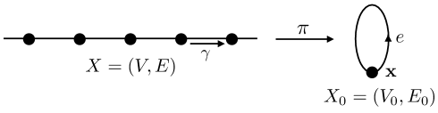
Figure 1. the 1-dimensional crystal lattice and its quotient graph.

A periodic realization $\Phi:V\to\mathbb{R}$ is naturally defined by $\Phi(0)=0$ and $\Phi(1)=1$. We identify $\gamma\in\Gamma$ with $1\in\mathbb{R}$ and put $\mathcal{J}=\{c=ka\,|\,k\in\mathbb{R},\,a\in\Phi(V)=\mathbb{Z}\}$.

Let $m=r=2$, $\lambda_{\ell j}=\delta_{\ell j},\,u_{j}=1,\,\ell,j=1,2$ and $c_{1},c_{2}\in\mathcal{J}$. We consider a multidimensional Shintani zeta function defined by

$$Z_{S}^{X,\Phi}(s):=\sum_{n_{1},n_{2}=0}^{\infty}\frac{\theta(n_{1},n_{2})}{(n_{1}+1)^{c_{1}s}(n_{2}+1)^{c_{2}s}},\qquad s\in\mathbb{C}.$$

(i) Let $j_{1},j_{2}$ be distinct positive integers greater than 1. Suppose that $c_{1}=-(\log j_{1})^{-1}$, $c_{2}=(\log j_{2})^{-1}$ and

$$\theta(n_{1},n_{2})=\begin{cases}\alpha\mathrm{e}^{-\sigma}&\text{if }(n_{1},n_{2})=(j_{1}-1,0)\\ \beta\mathrm{e}^{\sigma}&\text{if }(n_{1},n_{2})=(0,j_{2}-1)\\ 0&\text{otherwise}\end{cases},$$

where $\alpha,\beta\geq 0$, $\alpha+\beta=1$ and $\sigma>1$. Then we have

$$Z_{S}^{X,\Phi}(s)=\frac{\alpha\mathrm{e}^{-\sigma}}{j_{1}^{-(\log j_{1})^{-1}s}}+\frac{\beta\mathrm{e}^{\sigma}}{j_{2}^{(\log j_{2})^{-1}s}}=\alpha\mathrm{e}^{s-\sigma}+\beta\mathrm{e}^{-s+\sigma}$$

Therefore, the characteristic function $f_{\sigma}^{X,\Phi}(t)$ is given by

$$f_{\sigma}^{X,\Phi}(t)=\frac{Z_{S}^{X,\Phi}(\sigma+\mathrm{i}t)}{Z_{S}^{X,\Phi}(\sigma)}=\frac{\alpha\mathrm{e}^{\mathrm{i}t}+\beta\mathrm{e}^{-\mathrm{i}t}}{\alpha+\beta}=\alpha\mathrm{e}^{\mathrm{i}t}+\beta\mathrm{e}^{-\mathrm{i}t},\qquad t\in\mathbb{R},$$

which is that of $\mathbb{Z}$-valued random variable $\mathcal{Y}$ given by ${\bf P}(\mathcal{Y}=1)=\alpha$ and ${\bf P}(\mathcal{Y}=-1)=\beta$. This clearly induces the usual nearest-neighbor random walk on $\mathbb{Z}$ and also simple one when $\alpha=\beta=1/2$. Note that the random variable $\mathcal{Y}$ is not infinitely divisible.

(ii) Let $\lambda>0$ and $j>1$ be an integer. Suppose that $c_{1}=-(\log j)^{-1}$, $c_{2}=0$ and

$$\theta(n_{1},n_{2})=\begin{cases}1&\text{if }(n_{1},n_{2})=(0,0)\\ \lambda^{k}\mathrm{e}^{-k\sigma}/k!&\text{if }(n_{1},n_{2})=(j^{k}-1,0),\,k=1,2,\dots\\ 0&\text{otherwise}\end{cases},$$

where $\sigma>1$. Then we have

$$Z_{S}^{X,\Phi}(s)=\sum_{k=0}^{\infty}\frac{\lambda^{k}\mathrm{e}^{-k\sigma}/k!}{(j^{k})^{-(\log j)^{-1}s}}=\sum_{k=0}^{\infty}\frac{(\lambda\mathrm{e}^{s-\sigma})^{k}}{k!}=\exp(\lambda\mathrm{e}^{s-\sigma}).$$

Therefore, we obtain

$$f_{\sigma}^{X,\Phi}(t)=\frac{Z_{S}^{X,\Phi}(\sigma+\mathrm{i}t)}{Z_{S}^{X,\Phi}(\sigma)}=\frac{\exp(\lambda\mathrm{e}^{\mathrm{i}t})}{\exp(\lambda)}=\exp\big{(}\lambda(\mathrm{e}^{\mathrm{i}t}-1)\big{)},\qquad t\in\mathbb{R},$$

which corresponds to the usual Poisson random variable $\mathcal{Y}$ given by ${\bf P}(\mathcal{Y}=k)=\mathrm{e}^{-\lambda}\lambda^{k}/k!$ for $k=0,1,2,\dots$. Note that the random variable $\mathcal{Y}$ is infinitely divisible.

In the following, we discuss three typical examples of 2-dimensional crystal lattices and multiple zeta functions on them.

Example 5.2 (square lattice).

Let $d=2$ and $\Gamma=\langle\gamma_{1},\gamma_{2}\rangle$. We define $V=\mathbb{Z}^{2}$ and

$$E:=\big{\{}e=\{x,y\}\in\mathbb{Z}^{2}\times\mathbb{Z}^{2}\,|\,y-x\in\{(\pm 1,0),(0,\pm 1)\}\big{\}}.$$

The $\Gamma$-action on $X=(V,E)$ is given by $\gamma_{1}x:=x+(1,0)$ and $\gamma_{2}x:=x+(0,1)$ for $x\in V$. Then we easily see that the infinite graph $X$ is a $\Gamma$-covering of a 2-bouquet graph $X_{0}=(V_{0},E_{0})$, where $X_{0}=\{\bf{x}\}$ and $E_{0}=\{e_{1},e_{2},\overline{e}_{1},\overline{e}_{2}\}$ (see Figure 2). The first homology group $\mathrm{H}_{1}(X_{0},\mathbb{R})$ is given by $\{a_{1}[e_{1}]+a_{2}[e_{2}]\,|\,a_{1},a_{2}\in\mathbb{R}\},$ where $[e_{1}]$ and $[e_{2}]$ are homotopy classes of $e_{1}$ and $e_{2}$, respectively. Therefore, $X$ is maximal abelian.

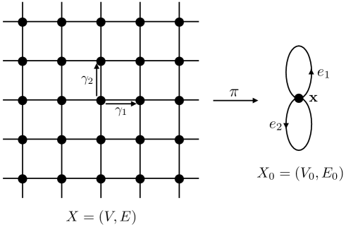
Figure 2. the 2-dimensional square lattice and its quotient graph.

A periodic realization $\Phi:V\to\mathbb{R}^{2}$ is defined by $\Phi\big{(}(0,0)\big{)}=(0,0)$ and

$$\Phi\big{(}(1,0)\big{)}=(1,0),\qquad\Phi\big{(}(0,1)\big{)}=(0,1).$$

We identify $\gamma_{1},\gamma_{2}\in\Gamma$ as vectors $(1,0),\,(0,1)\in\mathbb{R}^{2}$, respectively. We also define the sets of vectors $\mathcal{J}_{S}$ and $\mathcal{J}_{E}$ by

$$\mathcal{J}_{S}=\{\vec{c}=k\vec{a}\,|\,k\in\mathbb{R},\,\vec{a}\in\mathbb{Z}^{2}\},\quad\mathcal{J}_{E}=\big{\{}\vec{a}=k_{1}\gamma_{1}+k_{2}\gamma_{2}\,\big{|}\,k_{1},k_{2}\in\mathbb{Z}\big{\}}.$$

We consider a multidimensional Shintani zeta function and a multidimensional finite Euler product on $X$ given by

$$Z_{S}^{X,\Phi}(\vec{s}) :=\sum_{n_{1},n_{2},n_{3},n_{4}=0}^{\infty}\frac{\theta(n_{1},n_{2},n_{3},n_{4})}{\prod_{\ell=1}^{4}\big{(}\sum_{j=1}^{4}\lambda_{\ell j}(n_{j}+u_{j})\big{)}^{\langle\vec{c}_{\ell},\vec{s}\rangle}},\qquad\vec{s}\in\mathbb{C}^{2},$$ (5.1)

$$Z_{f\!E}^{X,\Phi}(\vec{s}) :=(1-\alpha_{1}\mathrm{e}^{-\langle\vec{a}_{1},\vec{s}\rangle})^{-1}(1-\alpha_{2}\mathrm{e}^{-\langle\vec{a}_{2},\vec{s}\rangle})^{-1},\qquad\vec{s}\in\mathbb{C}^{2},$$ (5.2)

where $\vec{c}_{1},\vec{c}_{2},\vec{c}_{3},\vec{c}_{4}\in\mathcal{J}_{S}$ and $\vec{a}_{1},\vec{a}_{2}\in\mathcal{J}_{E}$.

(i) Let $j_{1},j_{2},j_{3},j_{4}$ be four distinct positive integers greater than 1. Suppose that $\lambda_{\ell j}=\delta_{\ell j}$, $u_{j}=1$ for $\ell,j=1,2,3,4$, $\vec{c}_{1}=(-(\log j_{1})^{-1},0)$, $\vec{c}_{2}=((\log j_{2})^{-1},0)$, $\vec{c}_{3}=(0,-(\log j_{3})^{-1})$, $\vec{c}_{4}=(0,(\log j_{4})^{-1})$ and

$$\theta(n_{1},n_{2},n_{3},n_{4})=\begin{cases}\alpha\mathrm{e}^{-\sigma_{1}}&\text{if }(n_{1},n_{2},n_{3},n_{4})=(j_{1}-1,0,0,0)\\ \alpha\mathrm{e}^{\sigma_{1}}&\text{if }(n_{1},n_{2},n_{3},n_{4})=(0,j_{2}-1,0,0)\\ \beta\mathrm{e}^{-\sigma_{2}}&\text{if }(n_{1},n_{2},n_{3},n_{4})=(0,0,j_{3}-1,0)\\ \beta^{\prime}\mathrm{e}^{\sigma_{2}}&\text{if }(n_{1},n_{2},n_{3},n_{4})=(0,0,0,j_{4}-1)\\ 0&\text{otherwise}\end{cases}$$

as in (5.1), where $\alpha,\alpha^{\prime},\beta,\beta^{\prime}\geq 0$, $\alpha+\alpha^{\prime}+\beta+\beta^{\prime}=1$ and $\vec{\sigma}=(\sigma_{1},\sigma_{2})\in\mathbb{R}^{2}\setminus\{\bm{0}\}$. Then we have

$$Z_{S}^{X,\Phi}(\vec{s}) =\frac{\alpha\mathrm{e}^{-\sigma_{1}}}{j_{1}^{\langle\vec{c}_{1},\vec{s}\rangle}}+\frac{\alpha^{\prime}\mathrm{e}^{\sigma_{1}}}{j_{2}^{\langle\vec{c}_{2},\vec{s}\rangle}}+\frac{\beta\mathrm{e}^{-\sigma_{2}}}{j_{3}^{\langle\vec{c}_{3},\vec{s}\rangle}}+\frac{\beta^{\prime}\mathrm{e}^{\sigma_{2}}}{j_{4}^{\langle\vec{c}_{4},\vec{s}\rangle}}$$

$$=\alpha\mathrm{e}^{\langle(1,0),\vec{s}\rangle-\sigma_{1}}+\alpha^{\prime}\mathrm{e}^{\langle(-1,0),\vec{s}\rangle+\sigma_{1}}+\beta\mathrm{e}^{\langle(0,1),\vec{s}\rangle-\sigma_{2}}+\beta^{\prime}\mathrm{e}^{\langle(0,-1),\vec{s}\rangle-\sigma_{2}}.$$

By putting $\vec{s}=\vec{\sigma}+\mathrm{i}\vec{t}=(\sigma_{1},\sigma_{2})+\mathrm{i}(t_{1},t_{2})$ for $\vec{t}=(t_{1},t_{2})\in\mathbb{R}^{2}$, we obtain

$$f_{\vec{\sigma}}^{X,\Phi}(\vec{t})=\frac{Z_{S}^{X,\Phi}(\vec{\sigma}+\mathrm{i}\vec{t})}{Z_{S}^{X,\Phi}(\vec{\sigma})}=\alpha\mathrm{e}^{\mathrm{i}t_{1}}+\alpha^{\prime}\mathrm{e}^{-\mathrm{i}t_{1}}+\beta\mathrm{e}^{\mathrm{i}t_{2}}+\beta^{\prime}\mathrm{e}^{-\mathrm{i}t_{2}},$$

which is a characteristic function of a $\mathbb{Z}^{2}$-valued random variable $\mathcal{Y}$ given by

$${\bf P}(\mathcal{Y}=(1,0)) =\alpha,\quad {\bf P}(\mathcal{Y}=(-1,0)) =\alpha^{\prime},$$

$${\bf P}(\mathcal{Y}=(0,1)) =\beta,\quad {\bf P}(\mathcal{Y}=(0,-1)) =\beta^{\prime}.$$

This random variable induces a $\mathbb{Z}^{2}$-valued nearest-neighbor random walk and also a simple one when $\alpha=\alpha^{\prime}=\beta=\beta^{\prime}=1/4$.

(ii) Suppose that $\alpha_{1}=\alpha_{2}=1/3$, $\vec{a}_{1}=(1,0)$ and $\vec{a}_{2}=(0,1)$ as in (5.2). Then we have

$$Z_{f\!E}^{X,\Phi}(\vec{s})=\frac{3}{3-\mathrm{e}^{\langle(1,0),\vec{s}\rangle}}\cdot\frac{3}{3-\mathrm{e}^{\langle(0,1),\vec{s}\rangle}},\qquad\vec{s}\in\mathbb{C}^{2}.$$

It readily follows from Theorem 4.3 that, for $\vec{\sigma}:=(\log 2,\log 2)\in\mathbb{R}^{2}$, the function

$$f_{\vec{\sigma}}^{X,\Phi}(\vec{s})=\frac{Z_{f\!E}^{X,\Phi}(\vec{\sigma}+\mathrm{i}\vec{t})}{Z_{f\!E}^{X,\Phi}(\vec{\sigma})}=\frac{1}{(3-2\mathrm{e}^{\mathrm{i}t_{1}})(3-2\mathrm{e}^{\mathrm{i}t_{2}})},\qquad\vec{t}\in\mathbb{R}^{2},$$

is a compound Poisson characteristic function whose finite Lévy measure on $\mathbb{R}^{2}$ is given by

$$N_{\vec{\sigma}}^{X,\Phi}(d\vec{x})=\sum_{r=1}^{\infty}\frac{1}{r}\Big{(}\frac{2}{3}\Big{)}^{r}\big{(}\delta_{(r,0)}(d\vec{x})+\delta_{(0,r)}(d\vec{x})\big{)}.$$

Note that we have $N_{\vec{\sigma}}^{X,\Phi}(\mathbb{R}^{2})=2\log{3}$. This clearly induces a compound Poisson random variable $\Phi(\mathcal{Y}_{\vec{\sigma}})=\sum_{k=1}^{K_{\vec{\sigma}}^{X,\Phi}}\mathcal{X}_{k}$, where $\{\mathcal{X}_{k}\}_{k=1}^{\infty}$ is a family of $\mathbb{R}^{2}$-valued independent and identically distributed random variables whose common distribution is given by

$${\bf P}\big{(}\mathcal{X}_{1}=(r,0)\big{)}={\bf P}\big{(}\mathcal{X}_{1}=(0,r)\big{)}=\frac{1}{r}\Big{(}\frac{2}{3}\Big{)}^{r}\cdot\frac{1}{2\log 3},\qquad r\in\mathbb{N},$$

and $K_{\vec{\sigma}}^{X,\Phi}$ is a Poisson random variable with a parameter $2\log{3}$ independent of $\{\mathcal{X}_{k}\}_{k=1}^{\infty}$. The $n$-fold convolution of the distribution of the random variable $\Phi(\mathcal{Y})$ induces an infinite range random walk $\{\mathcal{W}_{n}\}_{n=0}^{\infty}$ generated by $Z_{f\!E}^{X,\Phi}$ whose characteristic function is

$$\mathbb{E}[\mathrm{e}^{\mathrm{i}\langle\vec{t},\Phi(\mathcal{W}_{n})\rangle}]=\big{(}f_{\vec{\sigma}}^{X,\Phi}(\vec{t})\big{)}^{n}=\frac{1}{(3-2\mathrm{e}^{\mathrm{i}t_{1}})^{n}(3-2\mathrm{e}^{\mathrm{i}t_{2}})^{n}},\qquad n\in\mathbb{N},\,\vec{t}=(t_{1},t_{2})\in\mathbb{R}^{2},$$

with $\Phi(\mathcal{W}_{0})=\bm{0}$.

Example 5.3 (triangular lattice).

Let $d=2$ and $\Gamma=\langle\gamma_{1},\gamma_{2}\rangle$. We define $V=\mathbb{Z}^{2}$ and

$$E:=\big{\{}e=\{x,y\}\in\mathbb{Z}^{2}\times\mathbb{Z}^{2}\,|\,y-x\in\{(\pm 1,0),(0,\pm 1),(\pm 1,\mp 1)\}\big{\}}.$$

The $\Gamma$-action on $X=(V,E)$ is given by $\gamma_{1}x:=x+(1,0)$ and $\gamma_{2}x:=x+(0,1)$ for $x\in V$. Then we see that $X$ is a $\Gamma$-covering of a 3-bouquet graph $X_{0}=(V_{0},E_{0})$, where $X_{0}=\{\bf{x}\}$ and $E_{0}=\{e_{1},e_{2},e_{3},\overline{e}_{1},\overline{e}_{2},\overline{e}_{3}\}$ (see Figure 3). Since the first homology group $\mathrm{H}_{1}(X_{0},\mathbb{R})$ is of dimension 3, it is known that $X$ is not maximal abelian.

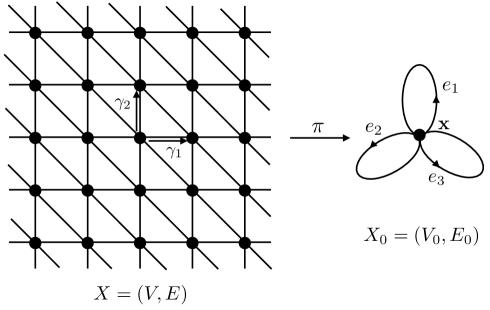
Figure 3. the triangular lattice and its quotients graph.

We take a periodic realization $\Phi:V\to\mathbb{R}^{2}$ and the set of vectors $\mathcal{J}_{S}$ as in the previous example. Let $N\in\mathbb{N}$ and

$$\mathcal{M}:=\{\vec{k}=(k_{1},k_{2})\in\mathbb{Z}^{2}\,:\,|k_{1}+k_{2}|\leq N,\,|k_{1}|,|k_{2}|\leq N\},$$

which is denoted by $\mathcal{M}=\{\vec{k}_{\ell}\}_{\ell=1}^{M}$ for a notational convention, where $M:=|\mathcal{M}|=3N^{2}+3N+1$. See Figure 4 below.

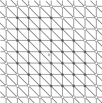
Figure 4. the set $\mathcal{M}$ in the case where $N=3$.

Let us consider a multidimensional Shintani zeta function on $X$ given by

$$Z_{S}^{X,\Phi}(\vec{s}) :=\sum_{n_{1},n_{2},\dots,n_{M}=0}^{\infty}\frac{\theta(n_{1},n_{2},\dots,n_{M})}{\prod_{\ell=1}^{M}(n_{\ell}+1)^{\langle\vec{c}_{\ell},\vec{s}\rangle}},\qquad\vec{s}\in\mathbb{C}^{2},$$ (5.3)

where $\vec{c}_{\ell}\in\mathcal{J}_{S}$ for $\ell=1,2,\dots,M$. Let $\alpha(\vec{k}),\,\vec{k}\in\mathcal{M}$ be real numbers taking values in the interval $(0,1)$ satisfying $\sum_{\vec{k}\in\mathcal{M}}\alpha(\vec{k})=1$ and $j_{\ell},\,\ell=1,2,\dots,M$, be distinct positive integers greater than 1. Suppose that $\vec{c}_{\ell}=-(\log j_{\ell})^{-1}\vec{k}_{\ell},\,\ell=1,2,\dots,M$, and

$$\theta(n_{1},n_{2},\dots,n_{M})$$

$$=\begin{cases}\alpha(\vec{k}_{\ell})\mathrm{e}^{-\langle\vec{k}_{\ell},\vec{\sigma}\rangle}&\text{if }(n_{1},\dots,n_{\ell},\dots,n_{M})=(0,\dots,0,j_{\ell}-1,0,\dots,0),\,\ell=1,2,\dots,M\\ 0&\text{otherwise}\end{cases},$$

where $\vec{\sigma}\in\mathbb{R}^{2}\setminus\{\bm{0}\}$. Then we have

$$Z_{S}^{X,\Phi}(\vec{s})=\sum_{\ell=1}^{M}\frac{\alpha(\vec{k}_{\ell})\mathrm{e}^{-\langle\vec{k}_{\ell},\vec{\sigma}\rangle}}{j_{\ell}^{\langle\vec{c}_{\ell},\vec{s}\rangle}}=\sum_{\vec{k}\in\mathcal{M}}\alpha(\vec{k})\mathrm{e}^{\langle\vec{k},\vec{s}-\vec{\sigma}\rangle}$$

and

$$f_{\vec{\sigma}}^{X,\Phi}(\vec{t})=\frac{Z_{S}^{X,\Phi}(\vec{\sigma}+\mathrm{i}\vec{t})}{Z_{S}^{X,\Phi}(\vec{\sigma})}=\sum_{\vec{k}\in\mathcal{M}}\alpha(\vec{k})\mathrm{e}^{\mathrm{i}\langle\vec{k},\vec{t}\rangle},\qquad\vec{t}\in\mathbb{R}^{2}.$$

Consequently, it is known that the $\mathbb{R}^{2}$-valued random variable $\mathcal{Y}$ whose characteristic function is $f_{\vec{\sigma}}^{X,\Phi}$ is represented as ${\bf P}(\mathcal{Y}=\vec{k})=\alpha(\vec{k}),\,\vec{k}\in\mathcal{M}$. This means that the random walk $\{\mathcal{W}_{n}\}_{n=0}^{\infty}$ generated by $Z_{S}^{X,\Phi}$ can visit all vertices whose graph distance from the current position is less than or equal to $N$ at each step.

Example 5.4 (hexagonal lattice).

Let $d=2$ and $\Gamma=\langle\gamma_{1},\gamma_{2}\rangle$. We define

$$V :=\mathbb{Z}^{2}=\{x=(x_{1},x_{2})\,|\,x_{1},x_{2}\in\mathbb{Z}\},$$

$$E :=\big{\{}e=\{x,y\}\in\mathbb{Z}^{2}\times\mathbb{Z}^{2}\,|\,y-x=(\pm 1,0),(0,(-1)^{x_{1}+x_{2}})\big{\}}.$$

The $\Gamma$-action on $X=(V,E)$ is given by $\gamma_{1}x:=x+(1,1)$ and $\gamma_{2}x:=x+(-1,1)$ for $x\in V$. Then $X$ is a covering graph of a finite graph $X_{0}=(V_{0},E_{0})$ with the covering transformation group $\Gamma$, where $X_{0}=\{\bf{x},{\bf y}\}$ and $E_{0}=\{e_{1},e_{2},e_{3},\overline{e}_{1},\overline{e}_{2},\overline{e}_{3}\}$ (see Figure 5). Since the first homology group $\mathrm{H}_{1}(X_{0},\mathbb{R})$ is of dimension 2, we see that $X$ is a maximal abelian covering graph as well as the square lattice.

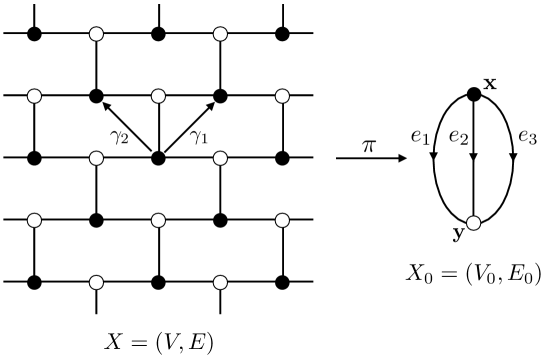
Figure 5. the hexagonal lattice and its quotients graph.

A periodic realization $\Phi:V\to\mathbb{R}^{2}$ is defined as in the following. We put $\widetilde{x}=(0,0)$ and $\widetilde{y}=(0,1)$ in $V$ and let $\Phi(\widetilde{x})=\bm{0}$ and $\Phi(\widetilde{y})=(1/3,2/3)$. Moreover, $\gamma_{1},\gamma_{2}\in\Gamma$ are identified with $(1,0),(0,1)\in\mathbb{R}^{2}$, respectively (see Figure 6).

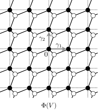
Figure 6. a periodic realization of the hexagonal lattice.

We define $\mathcal{J}(\Phi;{\bf x})$ and $\mathcal{J}(\Phi;{\bf y})$ by (3.1), respectively. For ${\bf x},{\bf y}\in V_{0}$, consider two multidimensional Shintani zeta functions given by

$$Z_{S}^{X,\Phi}({\bf x},\vec{s}):=\sum_{n_{1},n_{2},n_{3}=0}^{\infty}\frac{\theta_{{\bf x}}(n_{1},n_{2},n_{3})}{\prod_{\ell=1}^{3}\big{(}\sum_{j=1}^{3}\lambda_{\ell j}(n_{j}+1)\big{)}^{\langle\vec{c}_{\ell}({\bf x}),\vec{s}\rangle}},\qquad\vec{s}\in\mathbb{C}^{2},$$

$$Z_{S}^{X,\Phi}({\bf y},\vec{s}):=\sum_{n_{1},n_{2},n_{3}=0}^{\infty}\frac{\theta_{{\bf y}}(n_{1},n_{2},n_{3})}{\prod_{\ell=1}^{3}\big{(}\sum_{j=1}^{3}\lambda_{\ell j}(n_{j}+1)\big{)}^{\langle\vec{c}_{\ell}({\bf y}),\vec{s}\rangle}},\qquad\vec{s}\in\mathbb{C}^{2},$$

where $\vec{c}_{\ell}({\bf x})\in\mathcal{J}(\Phi;{\bf x})$ and $\vec{c}_{\ell}({\bf y})\in\mathcal{J}(\Phi;{\bf y})$ for $\ell=1,2,3$.

Let $j_{1},j_{2},j_{3}$ be distinct positive integers greater than 1. Suppose that $\lambda_{\ell j}=\delta_{\ell j}$ for $\ell,j=1,2,3$,

$$\vec{c}_{1}({\bf x}) =\Big{(}-\frac{1}{3}(\log j_{1})^{-1},-\frac{2}{3}(\log j_{1})^{-1}\Big{)}, \vec{c}_{2}({\bf x}) =\Big{(}-\frac{1}{3}(\log j_{2})^{-1},\frac{1}{3}(\log j_{2})^{-1}\Big{)},$$

$$\vec{c}_{3}({\bf x}) =\Big{(}\frac{2}{3}(\log j_{3})^{-1},\frac{1}{3}(\log j_{3})^{-1}\Big{)}, \vec{c}_{1}({\bf y}) =\Big{(}\frac{1}{3}(\log j_{1})^{-1},\frac{2}{3}(\log j_{1})^{-1}\Big{)},$$

$$\vec{c}_{2}({\bf y}) =\Big{(}\frac{1}{3}(\log j_{2})^{-1},-\frac{1}{3}(\log j_{2})^{-1}\Big{)}, \vec{c}_{3}({\bf y}) =\Big{(}-\frac{2}{3}(\log j_{3})^{-1},-\frac{1}{3}(\log j_{3})^{-1}\Big{)}$$

and

$$\theta_{{\bf x}}(n_{1},n_{2},n_{3})=\begin{cases}\alpha_{1}\mathrm{e}^{-\langle(\frac{1}{3},\frac{2}{3}),\vec{\sigma}({\bf x})\rangle}&\text{if }(n_{1},n_{2},n_{3})=(j_{1}-1,0,0)\\ \alpha_{2}\mathrm{e}^{-\langle(\frac{1}{3},-\frac{1}{3}),\vec{\sigma}({\bf x})\rangle}&\text{if }(n_{1},n_{2},n_{3})=(0,j_{2}-1,0)\\ \alpha_{3}\mathrm{e}^{-\langle(-\frac{2}{3},-\frac{1}{3}),\vec{\sigma}({\bf x})\rangle}&\text{if }(n_{1},n_{2},n_{3})=(0,0,j_{3}-1)\\ 0&\text{otherwise}\end{cases},$$

$$\theta_{{\bf y}}(n_{1},n_{2},n_{3})=\begin{cases}\beta_{1}\mathrm{e}^{-\langle(-\frac{1}{3},-\frac{2}{3}),\vec{\sigma}({\bf y})\rangle}&\text{if }(n_{1},n_{2},n_{3})=(j_{1}-1,0,0)\\ \beta_{2}\mathrm{e}^{-\langle(-\frac{1}{3},\frac{1}{3}),\vec{\sigma}({\bf y})\rangle}&\text{if }(n_{1},n_{2},n_{3})=(0,j_{2}-1,0)\\ \beta_{3}\mathrm{e}^{-\langle(\frac{2}{3},\frac{1}{3}),\vec{\sigma}({\bf y})\rangle}&\text{if }(n_{1},n_{2},n_{3})=(0,0,j_{3}-1)\\ 0&\text{otherwise}\end{cases},$$

where $\alpha_{1},\alpha_{2},\alpha_{3},\beta_{1},\beta_{2},\beta_{3}\geq 0$, $\alpha_{1}+\alpha_{2}+\alpha_{3}=\beta_{1}+\beta_{2}+\beta_{3}=1$ and $\vec{\sigma}({\bf x}),\vec{\sigma}({\bf y})\in\mathbb{R}^{2}\setminus\{\bm{0}\}$. Then we obtain

$$Z_{S}^{X,\Phi}({\bf x},\vec{s}) =\frac{\alpha_{1}\mathrm{e}^{-\langle(\frac{1}{3},\frac{2}{3}),\vec{\sigma}({\bf x})\rangle}}{j_{1}^{\langle\vec{c}_{1}({\bf x}),\vec{s}\rangle}}+\frac{\alpha_{2}\mathrm{e}^{-\langle(\frac{1}{3},-\frac{1}{3}),\vec{\sigma}({\bf x})\rangle}}{j_{2}^{\langle\vec{c}_{2}({\bf x}),\vec{s}\rangle}}+\frac{\alpha_{3}\mathrm{e}^{-\langle(-\frac{2}{3},-\frac{1}{3}),\vec{\sigma}({\bf x})\rangle}}{j_{3}^{\langle\vec{c}_{3}({\bf x}),\vec{s}\rangle}}$$

$$=\alpha_{1}\mathrm{e}^{\langle(\frac{1}{3},\frac{2}{3}),\vec{s}-\vec{\sigma}({\bf x})\rangle}+\alpha_{2}\mathrm{e}^{\langle(\frac{1}{3},-\frac{1}{3}),\vec{s}-\vec{\sigma}({\bf x})\rangle}+\alpha_{3}\mathrm{e}^{\langle(-\frac{2}{3},-\frac{1}{3}),\vec{s}-\vec{\sigma}({\bf x})\rangle},$$

$$Z_{S}^{X,\Phi}({\bf y},\vec{s}) =\frac{\beta_{1}\mathrm{e}^{-\langle(-\frac{1}{3},-\frac{2}{3}),\vec{\sigma}({\bf x})\rangle}}{j_{1}^{\langle\vec{c}_{1}({\bf x}),\vec{s}\rangle}}+\frac{\beta_{2}\mathrm{e}^{-\langle(-\frac{1}{3},\frac{1}{3}),\vec{\sigma}({\bf y})\rangle}}{j_{2}^{\langle\vec{c}_{2}({\bf y}),\vec{s}\rangle}}+\frac{\beta_{3}\mathrm{e}^{-\langle(\frac{2}{3},\frac{1}{3}),\vec{\sigma}({\bf x})\rangle}}{j_{3}^{\langle\vec{c}_{3}({\bf y}),\vec{s}\rangle}}$$

$$=\beta_{1}\mathrm{e}^{\langle(-\frac{1}{3},-\frac{2}{3}),\vec{s}-\vec{\sigma}({\bf y})\rangle}+\beta_{2}\mathrm{e}^{\langle(-\frac{1}{3},\frac{1}{3}),\vec{s}-\vec{\sigma}({\bf y})\rangle}+\beta_{3}\mathrm{e}^{\langle(\frac{2}{3},\frac{1}{3}),\vec{s}-\vec{\sigma}({\bf y})\rangle}.$$

Therefore, one has

$$f_{\vec{\sigma}({\bf x})}(\vec{t}) =\frac{Z_{S}^{X,\Phi}(\vec{\sigma}({\bf x})+\mathrm{i}\vec{t})}{Z_{S}^{X,\Phi}(\vec{\sigma}({\bf x}))}=\alpha_{1}\mathrm{e}^{\mathrm{i}(\frac{1}{3}t_{1}+\frac{2}{3}t_{2})}+\alpha_{2}\mathrm{e}^{\mathrm{i}(\frac{1}{3}t_{1}-\frac{1}{3}t_{2})}+\alpha_{3}\mathrm{e}^{\mathrm{i}(-\frac{2}{3}t_{1}-\frac{1}{3}t_{2})},$$

$$f_{\vec{\sigma}({\bf y})}(\vec{t}) =\frac{Z_{S}^{X,\Phi}(\vec{\sigma}({\bf y})+\mathrm{i}\vec{t})}{Z_{S}^{X,\Phi}(\vec{\sigma}({\bf y}))}=\beta_{1}\mathrm{e}^{\mathrm{i}(-\frac{1}{3}t_{1}-\frac{2}{3}t_{2})}+\beta_{2}\mathrm{e}^{\mathrm{i}(-\frac{1}{3}t_{1}+\frac{1}{3}t_{2})}+\beta_{3}\mathrm{e}^{\mathrm{i}(\frac{2}{3}t_{1}+\frac{1}{3}t_{2})},$$

for $\vec{t}=(t_{1},t_{2})\in\mathbb{R}^{2}$. These characteristic functions corresponds to the $\mathbb{R}^{2}$-valued random variables $\mathcal{Y}_{{\bf x}}$ and $\mathcal{Y}_{{\bf y}}$ given by

$${\bf P}\Big{(}\mathcal{Y}_{{\bf x}}=\Big{(}\frac{1}{3},\frac{2}{3}\Big{)}\Big{)}=\alpha_{1},\quad{\bf P}\Big{(}\mathcal{Y}_{{\bf x}}=\Big{(}\frac{1}{3},-\frac{1}{3}\Big{)}\Big{)}=\alpha_{2},\quad{\bf P}\Big{(}\mathcal{Y}_{{\bf x}}=\Big{(}-\frac{2}{3},-\frac{1}{3}\Big{)}\Big{)}=\alpha_{3}$$

and

$${\bf P}\Big{(}\mathcal{Y}_{{\bf y}}=\Big{(}-\frac{1}{3},-\frac{2}{3}\Big{)}\Big{)}=\beta_{1},\quad{\bf P}\Big{(}\mathcal{Y}_{{\bf y}}=\Big{(}-\frac{1}{3},\frac{1}{3}\Big{)}\Big{)}=\beta_{2},\quad{\bf P}\Big{(}\mathcal{Y}_{{\bf y}}=\Big{(}\frac{2}{3},\frac{1}{3}\Big{)}\Big{)}=\beta_{3},$$

respectively, which means that the random walk $\{\mathcal{W}_{n}\}_{n=0}^{\infty}$ on $X$ generated by the multidimensional Shintani zeta functions is the usual nearest-neighbor one and also the simple one if $\alpha_{1}=\alpha_{2}=\alpha_{3}=\beta_{1}=\beta_{2}=\beta_{3}=1/3$.

References

- [AN13a] T. Aoyama and T. Nakamura: Behaviors of multivariable finite Euler products in probabilistic view, Math. Nachr. 286 (2013), pp. 1691–1700.
- [AN13b] T. Aoyama and T. Nakamura: Multidimensional Shintani zeta functions and zeta distributions on , Tokyo J. Math. 36 (2013), pp. 521–538.
- [AN13c] T. Aoyama and T. Nakamura: Multidimensional polynomial Euler products and infinitely divisible distributions on , preprint (2013), available at arXiv:1204.4041.
- [Apo90] M. Apostol: Modular functions and Dirichlet series in Number Theory, Graduate Texts in Mathematics 41, Springer, 1990.
- [BPY01] P. Biane, J. Pitman and M. Yor: Probability laws related to the Jacobi theta and Riemann zeta functions, and Brownian excursions, Bull. Amer. Math. Soc. 38 (2001), pp. 435–465.
- [BHNY08] P. Bourgade, C. P. Hughes, A. Nikeghbali and M. Yor: The characteristic polynomial of a random unitary matrix: A probabilistic approach, Duke Math. J. 145 (2008), pp. 45–69.
- [GK68] B. V. Gnedenko and A. N. Kolmogorov: Limit Distributions for Sums of Independent Random Variables (Translated from the Russian by Kai Lai Chung), Addison-Wesley, 1968.
- [GIL08] D. Guido, T. Isola and M. L. Lapidus: Ihara’s zeta function for periodic graphs and its application in the amenable case, J. Funct. Anal. 255 (2008), pp. 1339–1361.
- [Iha66] Y. Ihara: On discrete subgroups of the two by two projective linear group over p-adic fields, J. Math. Soc. Japan 18 (1966), pp. 219–235.
- [IKK17] S. Ishiwata, H. Kawabi and M. Kotani: Long time asymptotics of non-symmetric random walks on crystal lattices, J. Funct. Anal. 272 (2017), pp.1553–1624.
- [JW35] B. Jessen and A. Wintner: Distribution functions and the Riemann zeta function, Trans. Amer. Math. Soc. 38 (1935), pp. 48–88.
- [Khi38] A. Ya. Khinchine: Limit Theorems for Sums of Independent Random Variables (in Russian), Moscow and Leningrad, 1938.
- [KS00a] M. Kotani and T. Sunada: Standard realizations of crystal lattices via harmonic maps, Trans. Amer. Math. Soc. 353 (2000), pp. 1–20.
- [KS00b] M. Kotani and T. Sunada: Albanese maps and off diagonal long time asymptotics for the heat kernel, Comm. Math. Phys. 209 (2000), pp. 633–670.
- [KS00b] M. Kotani and T. Sunada: Zeta functions of finite graphs, J. Math. Sci. Univ. Tokyo 7 (2000), pp. 7–25.
- [KS06] M. Kotani and T. Sunada: Large deviation and the tangent cone at infinity of a crystal lattice, Math. Z. 254 (2006), pp. 837–870.
- [LPS19] D. Lenz, F. Pogorzelski and M. Schmidt: Ihara zeta functions for infinite graphs, Trans. Amer. Math. Soc. 371 (2019), pp. 5687–5729.
- [LH01] G. Lin and C. Hu: The Riemann zeta distribution, Bernoulli 7 (2001) pp. 817–828.
- [Nak16] T. Nakamura, Zeta distributions generated by multidimensional polynomial Euler products with complex coefficients, preprint (2016), available at arXiv:1606.09418.
- [Sat99] K. Sato: Lévy Processes and Infinitely Divisible Distributions, Cambridge University Press, 1999.
- [Sun13] T. Sunada: Topological Crystallography: With a View Towards Discrete Geometric Analysis, Surveys and Tutorials in the Applied Mathematical Sciences 6, Springer Japan, 2013.
- [Ste07] J. Steuding: Value-Distribution of -functions, Lecture Notes in Mathematics 1887, Springer, Berlin, 2007.
- [Ter10] A. Terras: Zeta Functions of Graphs, Cambridge University Press, 2010.
- [Woe00] W. Woess: Random Walks on Infinite Graphs and Groups, Cambridge University Press, 2000.