Entropy production in longitudinally expanding Yang-Mills field with use of Husimi function — semiclassical approximation

Abstract

We investigate the possible thermalization process of the highly occupied and weakly coupled Yang-Mills fields expanding along the beam axis through an evaluation of the entropy, particle number, and pressure anisotropy. The time evolution of the system is calculated by solving the equation of motion for the Wigner function in the semiclassical approximation with initial conditions mimicking the glasma. For the evaluation of the entropy, we adopt the Husimi-Wehrl (HW) entropy, which is obtained by using the Husimi function, a positive semidefinite quantum distribution function given by smearing the Wigner function. By numerical calculations at $g=0.1$ and $0.2$, the entropy production is found to occur together with the particle creation in two distinct stages: In the first stage, the particle number and the entropy at low longitudinal momenta grow rapidly. In the second stage, the particle number and the entropy of higher longitudinal momentum modes show slower increase. The pressure anisotropy remains in our simulation and implies that the system is still out-of-equilibrium.

1 Introduction

Experimental studies at RHIC and LHC have provided phenomenological evidences of formation of strongly coupled matter soon after the collisions of relativistic heavy ions, and its evolution is well described by the hydrodynamics. The shear viscosity of the fluid in those successful hydrodynamical models is so small Perfect2000 ; Perfect2001_1 ; Perfect2001_2 ; Perfect2002 that the entropy produced in the hydrodynamical stage is estimated to be about only 10% of the total entropy EntropySH2008 ; EntropyMS2008 . Then most of the entropy is expected to be created before the formation of the fluid EntropyMS2011 . We have, however, only a poor grasp of the physical mechanism of such early entropy production within the underlying Quantum Chromodynamics. Thus it is indispensable to elucidate the entropy production mechanism in the pre-hydrodynamic stage for a deeper understanding of the outstanding problem of why the hydrodynamics becomes applicable at the short time after the collisions, $\tau\sim 0.6-1$ fm/c, known as the early thermalization puzzle Early2002 .

Shortly after the contact of two nuclei, the produced matter is understood as a highly occupied system consisting of weakly coupled but strongly interacting gluons  MV1994_1 ; MV1994_2 ; MV1994_3 ; LMW1995_1 ; LMW1995_2 . Such gluonic matter, called a glasma, initially consists of an approximately boost invariant color electric and color magnetic fields parallel to the collision axis. The fluctuations of this boost invariant fields grow exponentially due to instabilities of the Yang-Mills theory  Weibel1959 ; Mrowczynski1988 ; Mrowczynski1993 ; Mrowczynski2003 ; RS2003 ; RS2004 ; Arnold2003 ; Savvidy1997 ; Savvidy1978 ; Iwazaki2008 ; NO1978 ; FI2008 ; FIW2009 ; InstabilityCYM2006_1 ; InstabilityCYM2006_2 ; InstabilityCYM2006_3 ; InstabilityCYM2008 ; InstabilityCYM2009 ; InstabilityCYM2012FG ; InstabilityCYM2012BSSS ; InstabilityCYM2013 ; Tsutsui2015 ; Tsutsui2016 . The exponential growth of fluctuations should play a role in the isotropization of pressure in the glasma PressureDEGV2012 ; PressureEG2013 , and is also expected to drive entropy production in the glasma Tsukiji2016 ; Tsukiji2018 . Eventually, the grown Yang-Mills field is expected to decay into particles and to form hydrodynamic fluid.

In order to investigate the real-time dynamics of the glasma, a semiclassical method is widely used InstabilityCYM2006_3 ; InstabilityCYM2012FG ; PressureEG2013 ; Berges2014_1 ; Berges2014_2 ; BergesCSS2014 ; Tsukiji2018 . In this method, the classical field equation of motion is solved starting from the initial conditions containing quantum fluctuations, which is implemented to evaluate real-time evolution of a Wigner function, a Wigner-Weyl transform of a density matrix in terms of the field variables and their conjugate momenta. Such semiclassical description can be applied to real-time evolution of highly occupied and weakly coupled systems BergesCSS2014 , where a quantum effect gives only a small contribution.

It should be noted that some kind of coarse-graining is necessary in order to discuss thermalization in terms of the entropy based on the density matrix or the Wigner function or the classical phase space distribution function defined microscopically. Exact quantum evolution of a density matrix $\hat{\rho}$ is unitary, and thereby the von-Neumann entropy $S=-{\rm Tr}\rho\ln\rho$ stays constant. Analogously in classical systems, the phase space distribution function is constant along the classical trajectory and the Boltzmann entropy, $S=-\int dxdp/(2\pi)^{D}f\ln f$ with $D$ and $f$ being the number of degrees of freedom and the classical distribution function, stays constant due to the Liouville’s theorem. One of the ways to perform coarse-graining is to use the entanglement entropy entangle1 ; entangle2 , the von-Neumann entropy defined by a partially traced density matrix. The time evolution of the partially traced density matrix is non-unitary and then the entanglement entropy can grow in time. However, it is difficult to perform the partial trace for many-body systems such as a field theory. Another way is to use the entropy defined by the smeared density matrix or the Wigner function. The Husimi function, smeared Wigner function within the allowance of the uncertainty principle, is positive semidefinite and can be regarded as a probability density function in the phase space, and thus we can define the entropy based on the Husimi function, which we call the Husimi-Wehrl (HW) entropy Husimi1940 ; Wehrl1978 ; Wehrl1979 ; Kyoto2009 . The properties of the HW entropy in- and out-of-equilibrium have been studied analytically in some simple models: For a harmonic oscillator with a quanta $\hbar\omega$, the HW entropy for the Gibbs ensemble is larger than the von-Neumann entropy but tends to agree with that in the classical/high-temperature limit ($\hbar/T\to 0$) Kyoto2009 . In an inverted harmonic oscillator, the growth rate of the HW entropy asymptotically converges to the Kolmogorov-Sinai (KS) entropy, a sum of positive Lyapunov exponents Kyoto2009 , which implies that the production of the HW entropy is related to the chaoticity and instabilities in its classical counterpart. Both results suggest that the HW entropy can be a suitable guide to investigate thermalization at least in classical or semiclassical systems.

In this article, we evaluate the evolution of the Wigner function of the highly occupied and weakly coupled Yang-Mills fields with initial conditions mimicking the glasma in the semiclassical approximation, and analyze its thermalization in terms of the HW entropy that is obtained from the evaluated Wigner function. The semiclassical approximation method adopted here is essentially the same as the so-called classical statistical approximation  InstabilityCYM2006_3 ; InstabilityCYM2012FG ; PressureEG2013 ; Berges2014_1 ; Berges2014_2 ; BergesCSS2014 ; Tsukiji2018 in the sense that the initial conditions are sampled by Monte Carlo method and the classical equations of motion are solved. Our simulation is performed in the $\tau-\eta$ coordinate system, which represents a system expanding along the beam axis at the speed of light. In Refs. Tsukiji2016 ; Tsukiji2018 , the authors numerically showed that the HW entropy does grow definitely by the classical dynamics of the Yang-Mills field, and that the growth rate of the HW entropy is related to the intrinsic dynamics of the Yang-Mills theory, such as the chaoticity and instabilities. It should be noted, however, that the previous studies were only made in a static geometry with a focus on the thermalization by the intrinsic dynamics of the Yang-Mills field. Thus it would be intriguing to examine whether their findings are robust enough that they persist in an expanding geometry. The present work is an extension of the previous analysis to the expanding system with some technical improvements: We give an improved definition of the HW entropy in field theories that resolves two problems left unsolved in Refs. Tsukiji2016 ; Tsukiji2018 , over-counting gauge degrees of freedom and an ambiguity in choice of smearing parameters. Another important development in this article is the evaluation of the particle number and its relevance to the entropy production. The initial condition given as the glasma-like one with quantum fluctuations may be described as the coherent state. Then the deviation from the coherent state is realized in the subsequent time evolution. We give an operator representation of the particle number created due to this deviation, and investigate the relation of the entropy and particle number production. Moreover we provide a theoretical basis of the numerical method for a precise evaluation of the HW entropy by the test particle method, which was proposed in Refs. Tsukiji2016 .

This article is organized as follows. In Sec. 2, we introduce the semiclassical description of the real-time evolution of quantum systems based on the Wigner function, and give the definition of the HW entropy, using a simple example: one-dimensional quantum mechanics. In Sec. 3, we show how to numerically evaluate the HW entropy of a semiclassical field, using the scalar theory in the Minkowski spacetime. In Sec. 4, we investigate the dynamical production of the HW entropy in the semiclassical evolution of the $SU(2)$ Yang-Mills field in the expanding geometry. We also study other observables, pressure and particle number, and discuss the relation between the HW entropy and them. In Sec. 5, we summarize this article.

2 Formalism

In this section, we introduce the semiclassical description of the real-time evolution of quantum systems based on the Wigner function, and give the definition of the HW entropy, using a one-dimensional harmonic oscillator whose Hamiltonian reads $H=\hat{p}^{2}/2+\omega^{2}\hat{x}^{2}/2=\omega(\hat{a}^{{\dagger}}\hat{a}+1/2)$ with $\hat{a}=(\omega\hat{x}+i\hat{p})/\sqrt{2\omega}$.

2.1 Semiclassical description of Wigner function

The Wigner function is defined as the Wigner-Weyl transform of the density matrix $\hat{\rho}(t)$,

$$f_{\rm W}(x,p)\equiv\int{\rm d}y\left\langle x+\frac{y}{2}\mid\hat{\rho}(t)\mid x-\frac{y}{2}\right\rangle e^{-ipy}\ .$$ (1)

To describe the semiclassical evolution of the Wigner function, we use the classical limit of the von-Neumann equation,

$$\frac{\partial}{\partial t}f_{\rm W}(x,p)=\lim_{\hbar\to 0}\{\{H,f_{\rm W}(x,p)\}\}\ ,$$ (2)

where $\{\{,\}\}$ denotes the Moyal bracket. The Moyal bracket can be written as a power series of $\hbar^{2}$,

$$\{\{H,f_{\rm W}(x,p)\}\}=\{H,f_{\rm W}(x,p)\}+\mathcal{O}(\hbar^{2})\ ,$$ (3)

where $\{,\}$ denotes the Poisson bracket. In the classical limit ($\hbar\rightarrow 0$), therefore, Eq. (2) reads the same form as the Liouville equation that is an evolution equation of a classical distribution function,

$$\frac{\partial}{\partial t}f_{\rm W}(x,p)=\{H,f_{\rm W}(x,p)\}\ .$$ (4)

By combining the classical evolution equation given by Eq. (4) with the semiclassical initial condition given later in Eq. (7), we can describe the time-dependent Wigner function within the semiclassical approximation, where quantum fluctuation effects up to $\mathcal{O}(\hbar^{1})$ are included.

We calculate an expectation value of the given observable $\hat{\mathcal{O}}(\hat{x},\hat{p})$ through the following relation,

$$\left\langle\hat{\mathcal{O}}(\hat{x},\hat{p})\right\rangle={\rm Tr}\left(\hat{\mathcal{O}}(\hat{x},\hat{p})\hat{\rho}\right)=\int d\Gamma\ \mathcal{O}_{\rm W}(x,p)f_{\rm W}(x,p)\ ,$$ (5)

where $d\Gamma=dxdp/(2\pi)$ is the integration measure and $\mathcal{O}_{\rm W}(x,p)$ is the Wigner-Weyl transform of $\hat{\mathcal{O}}(\hat{x},\hat{p})$,

$$\mathcal{O}_{\rm W}(x,p)=\int{\rm d}y\left\langle x+\frac{y}{2}|\hat{\mathcal{O}}(\hat{x},\hat{p})|x-\frac{y}{2}\right\rangle e^{-ipy}\ .$$ (6)

In actual calculations in field theories, we may need to subtract the vacuum expectation value and others to obtain the well-defined observables as discussed later.

2.2 Wigner function of a coherent state

We use a coherent state for the initial condition in actual calculations discussed later, since a description with use of a coherent state is useful when the semiclassical approximation is valid. A coherent state is an eigenstate of the annihilation operator $\hat{a}|\alpha\rangle=\alpha|\alpha\rangle$, and is represented as $|\alpha\rangle=e^{-|\alpha|^{2}/2}e^{\alpha\hat{a}^{\dagger}}|0\rangle$ with $|0\rangle$ being the perturbative vacuum state; $\hat{a}|0\rangle=0$. The coherent state satisfies the minimum uncertainty relation, $\Delta x\Delta p=\frac{1}{2}$.  With use of the density matrix $\hat{\rho}:=|\alpha\rangle\langle\alpha|$, the Wigner function of the coherent state $|\alpha\rangle$ is given by

$$f_{\rm W}(x,p)= \int{\rm d}y\left\langle x+\frac{y}{2}\mid\alpha\right\rangle\left\langle\alpha\mid x-\frac{y}{2}\right\rangle e^{-ipy}=2\exp\left[-\frac{(x-\bar{x})^{2}}{2(\Delta x)^{2}}-\frac{(p-\bar{p})^{2}}{2(\Delta p)^{2}}\right]\ ,$$ (7)

where $\bar{x}$ and $\bar{p}$ are the expectation values of the position and momentum, respectively, and are related to the eigenvalue as $\alpha=(\omega\bar{x}+i\bar{p})/\sqrt{2\omega}$. The variances are given by $(\Delta x)^{2}:=\langle\alpha|(\hat{x}-\bar{x})^{2}|\alpha\rangle=1/(2\omega)$ and $(\Delta p)^{2}:=\langle\alpha|(\hat{p}-\bar{p})^{2}|\alpha\rangle=\omega/2$.

2.3 Husimi-Wehrl entropy

The Husimi function is obtained by smearing the Wigner function in the phase space within the allowance of the uncertainty principle,

$$f_{\rm H}(x,p,\sigma)\equiv\int{\rm d}\Gamma^{\prime}f_{\rm W}(x^{\prime},p^{\prime})G(x-x^{\prime},p-p^{\prime},\sigma)\ ,$$ (8)

where $G(x,p,\sigma)$ is the Gaussian smearing function,

$$G(x,p,\sigma)=2e^{-\sigma x^{2}-p^{2}/\sigma}\ ,$$ (9)

where $\sigma$ is the smearing parameter. The Husimi function is normalized in the phase space as $\int d\Gamma f_{\rm H}(x,p,\sigma)=1$. In addition, it is given as the expectation value of the density matrix in a coherent state $|\alpha;\sigma\rangle$ defined as the eigenstate of the annihilation operator $\hat{a}=(\sigma\hat{x}+i\hat{p})/\sqrt{2\sigma}$, $f_{\rm H}(x,p,\sigma)=\langle\alpha;\sigma\!\mid\!\hat{\rho}\!\mid\!\alpha;\sigma\rangle$, and is positive semidefinite unlike the Wigner function. Therefore, the Husimi function can be regarded as a probability distribution function in the phase space. Then, we can define the Husimi-Wehrl entropy as

$$S_{\rm HW}(\sigma)\equiv-\int{\rm d}\Gamma f_{\rm H}(x,p,\sigma)\ln{f_{\rm H}(x,p,\sigma)}\ .$$ (10)

While there exists an ambiguity of the choice of the smearing parameter $\sigma$ in the Husimi function, we unambiguously fix $\sigma$ by imposing physically natural requirement in the later section.

3 Husimi-Wehrl Entropy of scalar field in non-expanding geometry

Before proceeding with the study of the Yang-Mills field in the expanding geometry, we show how to numerically evaluate the HW entropy of a semiclassical field, using the scalar theory in Minkowski space-time as an example. All quantities in this section are normalized by a spatial lattice spacing $a$.

3.1 Scalar Field Theory on Lattice

We consider the massless $\phi^{4}$ theory on a $L^{3}$ lattice whose Hamiltonian is given by

$$H=\sum_{\bm{x}}\left[\frac{1}{2}\hat{\pi}(x)^{2}-\frac{1}{2}\left(\bm{\nabla}^{\rm F}\hat{\phi}(x)\right)^{2}+\frac{\lambda}{4!}\hat{\phi}^{4}(x)\right]\ ,$$ (11)

where $\bm{\nabla}^{\rm F}=(\partial^{\rm F}_{1},\partial^{\rm F}_{2},\partial^{\rm F}_{3})$ denotes a forward difference operator, and $\hat{\pi}=\dot{\hat{\phi}}$ is the canonical conjugate variable of $\hat{\phi}$. Then, field variables for the free scalar field ($\lambda=0$) on the lattice after the second quantization are given by

$$\hat{\phi}(x) =\frac{1}{\sqrt{L^{3}}}\sum_{\bm{k}}\hat{\phi}_{\bm{k}}e^{i\bm{k}\cdot\bm{x}}=\frac{1}{\sqrt{L^{3}}}\sum_{\bm{k}}\frac{1}{\sqrt{2\omega_{\bm{k}}}}\left(\hat{a}_{\bm{k}}e^{-i\omega_{\bm{k}}t}+\hat{a}^{\dagger}_{-\bm{k}}e^{i\omega_{\bm{k}}t}\right)e^{i\bm{k}\cdot\bm{x}}\ ,$$ (12)

$$\hat{\pi}(x) =\frac{1}{\sqrt{L^{3}}}\sum_{\bm{k}}\hat{\pi}_{\bm{k}}e^{i\bm{k}\cdot\bm{x}}=\frac{-i}{\sqrt{L^{3}}}\sum_{\bm{k}}\sqrt{\frac{\omega_{\bm{k}}}{2}}\left(\hat{a}_{\bm{k}}e^{-i\omega_{\bm{k}}t}-\hat{a}^{\dagger}_{-\bm{k}}e^{i\omega_{\bm{k}}t}\right)e^{i\bm{k}\cdot\bm{x}}\ ,$$ (13)

where $(\hat{\phi}_{\bm{k}},\hat{\pi}_{\bm{k}})$ are the Fourier transform of $(\hat{\phi}(x),\hat{\pi}(x))$, $\hat{a}_{\bm{k}}$ $(\hat{a}^{\dagger}_{\bm{k}})$ is the annihilation (creation) operator for the free scalar field satisfying $\left[\hat{a}_{\bm{k}},\hat{a}^{\dagger}_{\bm{k}^{\prime}}\right]=\delta_{\bm{k},\bm{k}^{\prime}}$, and $\omega_{\bm{k}}=2\sqrt{\sin^{2}(k_{1}/2)+\sin^{2}(k_{2}/2)+\sin^{2}(k_{3}/2)}$ is the eigenfrequency of the free field mode with momentum $\bm{k}$ on the lattice.

The free part of the scalar theory can be interpreted as a set of harmonic oscillators, whose Hamiltonian is given by

$$H_{\rm free}=\sum_{\bm{k}}\,\omega_{\bm{k}}\left(\hat{a}^{\dagger}_{\bm{k}}\hat{a}_{\bm{k}}+\frac{1}{2}\right)=\sum_{\bm{k}}H^{\rm h.o.}_{\bm{k}}\,,\ H^{\rm h.o.}_{\bm{k}}=\frac{1}{2}\hat{\Pi}_{\bm{k}}^{2}+\frac{1}{2}\omega^{2}_{\bm{k}}\hat{\Phi}_{\bm{k}}^{2}\,,$$ (14)

where we have introduced the new canonical variables for each momentum mode, $(\hat{\Phi}_{\bm{k}},\hat{\Pi}_{\bm{k}})$, utilizing the annihilation and creation operators as

$$\hat{\Phi}_{\bm{k}}\equiv\frac{1}{\sqrt{2\omega_{\bm{k}}}}\left[\hat{a}_{\bm{k}}+\hat{a}^{\dagger}_{\bm{k}}\right]\ ,\ \ \ \hat{\Pi}_{\bm{k}}\equiv-i\sqrt{\frac{\omega_{\bm{k}}}{2}}\left[\hat{a}_{\bm{k}}-\hat{a}^{\dagger}_{\bm{k}}\right]\ ,$$ (15)

or accordingly,

$$\hat{a}_{\bm{k}}=(\omega_{\bm{k}}\hat{\Phi}_{\bm{k}}+i\hat{\Pi}_{\bm{k}})/\sqrt{2\omega_{\bm{k}}}.$$ (16)

Now we can consider the Winger function $f_{\rm W}(\{\Phi,\Pi\})$ expressed in terms of $\Phi_{\bm{k}}$ and $\Pi_{\bm{k}}$. As the initial condition, we adopt the coherent state $|\{\alpha_{\bm{k}}\}\rangle$ that is the eigenstate of annihilation operators for the free scalar field, $\{\hat{a}_{\bm{k}}\}$, and is given by the product of coherent states of each mode, $|\{\alpha_{\bm{k}}\}\rangle=\prod_{\bm{k}}|\alpha_{\bm{k}}\rangle$. Accordingly, the density matrix is expressed as $\hat{\rho}(t)=|\{\alpha_{\bm{k}}\}\rangle\langle\{\alpha_{\bm{k}}\}|=\prod_{\bm{k}}|\alpha_{\bm{k}}\rangle\prod_{\bm{k}^{\prime}}\langle\alpha_{\bm{k}^{\prime}}|$. Then, as shown in Eq (7), the Wigner function at the initial time is given by the Gaussian function,

$$f_{\rm W}(\{\Phi,\Pi\}) =\prod_{\bm{k}}\int{\rm d}\Phi^{\prime}_{\bm{k}}\left\langle\Phi_{\bm{k}}+\frac{\Phi^{\prime}_{\bm{k}}}{2}\,\Big{|}\,\alpha_{\bm{k}}\right\rangle\left\langle\alpha_{\bm{k}}\,\Big{|}\,\Phi_{\bm{k}}-\frac{\Phi^{\prime}_{\bm{k}}}{2}\right\rangle e^{-i\Pi_{\bm{k}}\Phi^{\prime}_{\bm{k}}}$$

$$=\prod_{\bm{k}}2\exp\left[-\frac{(\Phi_{\bm{k}}-\bar{\Phi}_{\bm{k}})^{2}}{2(\Delta\Phi_{\bm{k}})^{2}}-\frac{(\Pi_{\bm{k}}-\bar{\Pi}_{\bm{k}})^{2}}{2(\Delta\Pi_{\bm{k}})^{2}}\right]\,,$$ (17)

where the expectation values, $\bar{\Phi}_{\bm{k}}$ and $\bar{\Pi}_{\bm{k}}$, are the real and imaginary parts of the coherent state eigenvalue, $\alpha_{\bm{k}}=(\omega_{\bm{k}}\bar{\Phi}_{\bm{k}}+i\bar{\Pi}_{\bm{k}})/\sqrt{2\omega_{\bm{k}}}$, and the variances, $(\Delta\Phi_{\bm{k}})^{2}$ and $(\Delta\Pi_{\bm{k}})^{2}$, are determined by the eigenfrequency $\omega_{\bm{k}}$ as $\omega_{\bm{k}}=1/[2(\Delta\Phi_{\bm{k}})^{2}]=2(\Delta\Pi_{\bm{k}})^{2}$. It is noted that the spread of the initial Wigner function characterized by the widths, $\Delta\Phi_{\bm{k}}$ and $\Delta\Pi_{\bm{k}}$, corresponds to the zero-point oscillation of the vacuum if fluctuations of fields are regarded as particles.

We further define a Husimi function $f_{H}$ as a smeared Wigner function with the smearing parameters $\{\sigma_{\bm{k}}\}$ set to eigenfrequencies $\{\omega_{\bm{k}}\}$,

$$f_{\rm H}(\{\Phi,\Pi,\omega\})=\int\mathcal{D}\Gamma^{\prime}f_{\rm W}(\{\Phi^{\prime},\Pi^{\prime}\})G(\{\Phi-\Phi^{\prime},\Pi-\Pi^{\prime},\omega\})\ ,$$ (18)

where $\mathcal{D}\Gamma=\prod_{\bm{k}}d\Phi_{\bm{k}}d\Pi_{\bm{k}}/(2\pi)$ is an integration measure and $G(\{\Phi,\Pi,\omega\})$ is the smearing function defined as the product of single Gaussian smearing functions given in Eq.(9),

$$G(\{\Phi,\Pi,\omega\})=\prod_{\bm{k}}G(\Phi_{\bm{k}},\Pi_{\bm{k}},\omega_{\bm{k}})\ .$$ (19)

The HW entropy is finally given by

$$S_{\rm HW}(\{\omega\})=-\int\mathcal{D}\Gamma f_{\rm H}(\{\Phi,\Pi,\omega\})\ln{f_{\rm H}(\{\Phi,\Pi,\omega\})}\ .$$ (20)

We here comment on the smearing parameter choice shown above. The HW entropy $S_{\rm HW}(\{\omega\})$ defined with the smearing parameter $\{\omega\}$ exhibits two remarkable and physically natural features, as shown in App. D, at $\lambda=0$: The HW entropy $S_{\rm HW}(\{\omega\})$ agrees with the von-Neumann entropy $S_{\rm vN}=-{\rm Tr}(\rho\ln\rho)$ in the high-temperature limit, and the HW entropy $S_{\rm HW}(\{\omega\})$ per degrees of freedom in vacuum is unity, the minimum of the HW entropy. These two features may justify to adopt the definition in weak coupling calculations. In the later discussion of this section, we omit $\{\omega\}$ in the expression of the HW entropy of the scalar field: $S_{\rm HW}$.

3.2 Numerical method

3.2.1 Evaluation of Wigner function using test particle method

In the actual evaluation of the Wigner function, we use the test particle (TP) method in which the Wigner function is approximated by a sum of the delta functions,

$$f_{\rm W}^{\rm TP}(\{\Phi,\Pi\})=\frac{1}{N_{\rm TP}}\sum_{i}\prod_{\bm{k}}(2\pi)\delta(\Phi_{\bm{k}}-\Phi_{\bm{k},i}(t))\delta(\Pi_{\bm{k}}-\Pi_{\bm{k},i}(t))\ ,$$ (21)

where each delta function specifies the coordinate of an independent particle $(\Phi_{\bm{k},i},\Pi_{\bm{k},i})$ which is generated so as to sample the classical field configurations (test particle configurations) according to the distribution of the Wigner function. The test particle method assumes the positive semi-definiteness of the Wigner function, which is certainly true in the time evolution of the Wigner function according to the Liouville equation shown in Eq. (4) starting from the positive definite initial condition like Eq. (17). The Winger function given in Eq. (21) should give an accurate sampling of the original Wigner function in the large $N_{\rm TP}$ limit.

The test particles at initial time are generated according to the initial Wigner function given in Eq (17),

$$\Phi_{\bm{k},i}=\bar{\Phi}_{\bm{k}}+\sqrt{\frac{1}{2\omega_{\bm{k}}}}\xi_{\bm{k},i}^{R}\,,\ \Pi_{\bm{k},i}=\bar{\Pi}_{\bm{k}}+\sqrt{\frac{\omega_{\bm{k}}}{2}}\xi_{\bm{k},i}^{I}\,,$$ (22)

where $\xi_{\bm{k},i}^{R,I}$ are the random numbers obeying the normal Gaussian distribution. The time evolution of each test particle is obtained by the classical equation of motion, $\dot{\phi}(x)=\partial H/\partial\pi(x),\dot{\pi}(x)=-\partial H/\partial\phi(x)$. In the later discussion, we calculate an expectation value of a given observable $\hat{\mathcal{O}}(\{\hat{\Phi},\hat{\Pi}\})$, such as pressure and particle number, by using the test particle expression of the Wigner function given in Eq. (5),

$$\left\langle\hat{\mathcal{O}}(\{\hat{\Phi},\hat{\Pi}\})\right\rangle=\frac{1}{N_{\rm TP}}\sum_{i}\mathcal{O}(\{\Phi_{i},\Pi_{i}\})\ .$$ (23)

3.2.2 Husimi-Wehrl entropy in test particle method

By substituting the Wigner function given in Eq. (21) into Eq. (18), we obtain the Husimi function in the test particle method,

$$f_{\rm H}^{\rm TP}(\{\Phi,\Pi\})=\frac{1}{N_{\rm TP}}\sum_{i}\prod_{\bm{k}}G_{\bm{k},i}(\Phi_{\bm{k}},\Pi_{\bm{k}})\,,$$ (24)

$$G_{\bm{k},i}(\Phi_{\bm{k}},\Pi_{\bm{k}})=G(\Phi_{\bm{k}}-\Phi_{\bm{k},i}(t),\Pi_{\bm{k}}-\Pi_{\bm{k},i}(t),\omega_{\bm{k}})\ .$$ (25)

Then the HW entropy in the test particle method is given by

$$S_{\rm HW}^{\rm TP}= -\int D\Gamma\left[\frac{1}{N_{\rm TP}}\sum_{i}\prod_{\bm{k}}G_{\bm{k},i}(\Phi_{\bm{k}},\Pi_{\bm{k}})\right]\ln{\left[\frac{1}{N_{\rm TP}}\sum_{j}\prod_{\bm{k}^{\prime}}G_{\bm{k}^{\prime},j}(\Phi_{\bm{k}^{\prime}},\Pi_{\bm{k}^{\prime}})\right]}\,.$$ (26)

The HW entropy is evaluated in the following three steps in our test particle method which is elaborated from that adopted in the previous work. In the first step, we apply identical test particle sets to functions both inside and outside the logarithmic function in Eq. (26), and evaluate the HW entropy. We call this prescription the ”single test particle method (sTP)”, and denote the HW entropy obtained by the sTP method as $S_{\rm HW}^{\rm sTP}$. In the second step, we compute the HW entropy using two different test particle sets for functions inside and outside the logarithmic function in Eq. (26). We call the second prescription the ”parallel test particle method (pTP)”, and denote the HW entropy obtained by the pTP method as $S_{\rm HW}^{\rm pTP}$. Finally, we estimate the HW entropy by averaging $S_{\rm HW}^{\rm sTP}$ and $S_{\rm HW}^{\rm pTP}$, $S_{\rm HW}^{\rm aTP}\equiv(S_{\rm HW}^{\rm sTP}+S_{\rm HW}^{\rm pTP})/2$. As proven in App. C, we obtain the following inequality,

$$S_{\rm HW}^{\rm sTP}<S_{\rm HW}<S_{\rm HW}^{\rm pTP}\ .$$ (27)

by assuming that numerical errors of the Husimi function, $\Delta^{\rm TP}=f_{\rm H}^{\rm TP}-f_{\rm H}\propto 1/\sqrt{N_{\rm TP}}$, is sufficiently small due to the large value of $N_{\rm TP}$, and that the odd-order contributions of $\Delta^{\rm TP}$ to $S_{\rm HW}^{\rm sTP}$ and $S_{\rm HW}^{\rm pTP}$ disappear due to the numerical error cancellation, Moreover, it is also shown in App. C that the numerical errors proportional to $N_{\rm TP}^{-1}$ cancel out each other in $S_{\rm HW}^{\rm aTP}$, and $S_{\rm HW}^{\rm aTP}$ only contains $\mathcal{O}(N_{\rm TP}^{-2})$ errors. Thus, for the sufficiently large $N_{\rm TP}$, the following nice equality holds,

$$S_{\rm HW}^{\rm aTP}=S_{\rm HW}+\mathcal{O}(N_{\rm TP}^{-2})\ .$$ (28)

In the next section, we numerically calculate $S_{\rm HW}^{\rm sTP}$, $S_{\rm HW}^{\rm pTP}$ and $S_{\rm HW}^{\rm aTP}$ at different numbers of test particles, and discuss the validity of Eq. (27) and Eq. (28).

3.2.3 Product ansatz

We need to make a further approximation, assuming the product ansatz for the Wigner function in order to obtain the HW entropy in Eq. (26) in the test particle method. While the Husimi function is equivalent to the expectation value of the density matrix in the coherent state and takes a value $0\leq f_{\rm H}\leq 1$, the Husimi function in the test particle method, Eq. (24), takes a value $f_{\rm H}\geq 2^{N_{D}}/N_{\rm TP}$ at one of the test particle phase-space coordinates, $(\Phi_{\bm{k}},\Pi_{\bm{k}})=(\Phi_{\bm{k},i},\Pi_{\bm{k},i})$, with $N_{D}=L^{3}$ being the number of degrees of freedom. Then the required number of test particles is $N_{\rm TP}>2^{N_{D}}$ in order to respect the $f_{\rm H}$ range. As in this example, in order to cover the $2N_{D}$ dimensional phase space, we need a huge number of test particles. We cannot prepare such sufficiently large numbers of test particle configurations for large $L$.

To circumvent this practical problem, we assume the product ansatz for the Wigner function, a la Hartree-Fock approach,

$$f_{\rm W}(\{\Phi,\Pi\})=\prod_{\bm{k}}f_{\rm W}^{\bm{k}}(\Phi_{\bm{k}},\Pi_{\bm{k}})\ ,\ \ \ f_{\rm W}^{\bm{k}}(\Phi_{\bm{k}},\Pi_{\bm{k}})=\frac{1}{N_{\rm TP}}\sum_{i}(2\pi)\delta(\Phi_{\bm{k}}-\Phi_{\bm{k},i})\delta(\Pi_{\bm{k}}-\Pi_{\bm{k},i})\ ,$$ (29)

which means that there is no correlation between the wave functions of different momentum modes. Under the product ansatz, the Husimi function is also nicely expressed as the product of that of the single momentum mode,

$$f_{\rm H}(\{\Phi,\Pi\})=\prod_{\bm{k}}f_{\rm H}^{\bm{k}}(\Phi_{\bm{k}},\Pi_{\bm{k}}),\ \ \ f_{\rm H}^{\bm{k}}(\Phi_{\bm{k}},\Pi_{\bm{k}})=\frac{1}{N_{\rm TP}}\sum_{i}G_{\bm{k},i}(\Phi_{\bm{k}},\Pi_{\bm{k}})\,,$$ (30)

which allows us to treat the multiple integration in Eq. (26) as the sum of double integrations,

$$S_{\rm HW}= \sum_{\bm{k}}S_{\rm HW}^{\bm{k}}\,,\ S_{\rm HW}^{\bm{k}}=-\int\frac{d\Phi_{\bm{k}}d\Pi_{\bm{k}}}{(2\pi)^{3}}f_{\rm H}^{\bm{k}}(\Phi_{\bm{k}},\Pi_{\bm{k}})\ln f_{\rm H}^{\bm{k}}(\Phi_{\bm{k}},\Pi_{\bm{k}})$$ (31)

The product ansatz does not necessarily hold in interacting systems, since the interaction generates correlations between different modes. The product ansatz for $f_{\rm H}$ in Eq. (30) tells us that $f_{\rm H}^{\bm{k}}$ is a partially traced distribution function,

$$f_{\rm H}^{\bm{k}}(\Phi_{\bm{k}},\Pi_{\bm{k}})=\int\prod_{\bm{k}^{\prime}\not=\bm{k}}\frac{d\Phi_{\bm{k}^{\prime}}d\Pi_{\bm{k}^{\prime}}}{2\pi}f_{\rm H}(\{\Phi,\Pi\})\,.$$ (32)

Thus while we aim at calculating the entropy from the coarse-graining, the HW entropy with the product ansatz given in Eq. (31) is found to overestimate it by the amount of the entropy resulting from the loss of the correlation caused by the partial trace of $f_{\rm H}$. So far, the entropy increase caused by the use of the product ansatz have been tested only for a few dimensional quantum system Tsukiji2016 , and the entropy increase in such a case is found to be around 20% of that from only the coarse-graining. However, the product ansatz is a kind of a mean-field approximation like the Hartree(-Fock) approximation, and is expected to provide a good approximation for a system with large degrees of freedom, such as a highly occupied system, where fluctuations should be small.

3.3 Numerical results

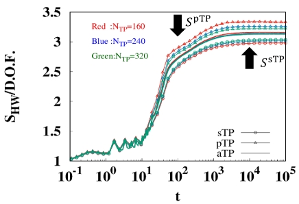
Figure 1: The time evolution of the HW entropy of the scalar field with $\lambda=1$ on the $16^{3}$ lattice. The red, blue and green line show the results for $N_{\rm TP}=160$, $240$ and $320$, respectively. The lines with circles, triangles, and no symbols show the HW entropy evaluated by the sTP method ($S_{\rm HW}^{\rm sTP}$), the pTP method ($S_{\rm HW}^{\rm pTP}$), and their average ($S_{\rm HW}^{\rm aTP}$), respectively.

Here we show the numerical results of the time evolution of the HW entropy of the scalar field theory using the product ansatz with the coupling constant $\lambda=1$ on the $16^{3}$ lattice with the periodic boundary condition. The initial positions of test particles in the phase space are generated according to the initial Wigner function given in Eq (17), where the initial macroscopic fields $(\bar{\Phi}_{\bm{k}},\bar{\Pi}_{\bm{k}})$ are given so as to satisfy the following simple initial condition,

$$\bar{\Phi}({\bm{x}})=5\sin{\left(\frac{\pi}{4}(x+y)\right)}\ ,\ \ \ \bar{\Pi}(\bm{x})=0\ .$$ (33)

The classical equation of motion for each test particle is solved by leapfrog integration. The number of test particles is taken as $N_{\rm TP}=160$, $240$ and $320$.

Figure 1 shows the evolution of $S_{\rm HW}^{\rm sTP}$, $S_{\rm HW}^{\rm pTP}$ and $S_{\rm HW}^{\rm aTP}$ per degrees of freedom at $N_{\rm TP}=160$, $240$ and $320$. It is found that $S_{\rm HW}^{\rm sTP}<S_{\rm HW}^{\rm pTP}$ always holds and the difference between $S_{\rm HW}^{\rm sTP}$ and $S_{\rm HW}^{\rm pTP}$ becomes smaller as $N_{\rm TP}$ increases, which is consistent with the inequality shown in Eq. (27). Moreover, the $N_{\rm TP}$ dependence of $S_{\rm HW}^{\rm aTP}$ at $N_{\rm TP}=160$, $240$ and $320$ is much smaller than those for $S_{\rm HW}^{\rm sTP}$ and $S_{\rm HW}^{\rm pTP}$, and is only less than 2%, which indicates that the equality shown in Eq. (28) holds. In what follows, we adopt $S_{\rm HW}^{\rm aTP}$ as the estimation of $S_{\rm HW}$, $S_{\rm HW}=S_{\rm HW}^{\rm aTP}$.

The time evolution of the HW entropy shows the relaxation processes from a coherent state to thermal equilibrium. At the initial time $t=0$, $S_{\rm HW}$ starts from unity, which reflects that the initial system is given by a coherent state. One sees that $S_{\rm HW}$ first increases rapidly, then shows only a gradual increase, and finally reaches some value and hardly changes. The saturation of $S_{\rm HW}$ indicates that the system reaches the thermal equilibrium. The final value of $S_{\rm HW}$ may be the HW entropy in the thermal equilibrium in the classical limit, which is estimated as

$$S_{\rm HW}^{\rm cl.eq.}\sim 3.1\ .$$ (34)

To compare with the thermal HW entropy shown in Eq. (34), we consider the classical Gibbs ensemble of the free field,

$$f_{\rm W}^{\rm cl.eq.}(\{\Phi,\Pi\})|_{\lambda=0}\propto e^{-H_{\rm free}/T}=\prod_{\bm{k}}\exp{\left[-\frac{\omega_{\bm{k}}^{2}\Phi^{2}_{\bm{k}}+\Pi^{2}_{\bm{k}}}{2T}\right]}\ ,$$ (35)

which gives thermal expectation values of observables in the classical limit at $\lambda=0$. Then, we get the Husimi function,

$$f_{\rm H}^{\rm cl.eq.}(\{\Phi,\Pi,\omega\})|_{\lambda=0}\propto\prod_{\bm{k}}\exp{\left[-\frac{\omega_{\bm{k}}^{2}\Phi^{2}_{\bm{k}}+\Pi^{2}_{\bm{k}}}{2(T+\omega_{\bm{k}}/2)}\right]}\ ,$$ (36)

and the HW entropy,

$$S_{\rm HW}^{\rm cl.eq.}|_{\lambda=0}=\sum_{\bm{k}}\left[1+\ln{\left(\frac{T+\omega_{\bm{k}}/2}{\omega_{\bm{k}}}\right)}\right]\ .$$ (37)

Assuming that the system is in the thermal equilibrium after the HW entropy stops to increase, we extract the temperature of the system through the equipartition relation $\left\langle\pi(x)^{2}\right\rangle=T$ that holds in thermal equilibrium in the classical limit. By substituting the numerically extracted temperature $T=20$ into Eq. (37), we obtain $S_{\rm HW}^{\rm cl.eq.}|_{\lambda=0}$ at the same temperature as our simulation, $S_{\rm HW}^{\rm cl.eq.}\Big{|}_{\lambda=0,T=20}\sim 3.2$. This theoretical estimate and our numerical estimation $S_{\rm HW}^{\rm cl.eq.}\Big{|}_{\lambda=1,T=20}\sim 3.1$ in Eq. (34) agree well with each other, and it indicates that our simulation parameter at $\lambda=1$ describes the relaxation to thermal equilibrium in the weak coupling region of the theory. Note that since the HW entropy shown in Eq. (37) is based on the classical thermal equilibrium distribution, its entropy density has the UV divergence in the continuum limit. To circumvent this problem, it is useful to use a framework that can perturbatively take account of higher-order quantum effects, including quantum statistical properties, such as the kinetic theory AMYkinetic and the two-particle irreducible (2PI) effective action approach Berges:2004yj ; Aarts:2001yn ; Hatta-Nishiyama . Aside from these descriptions, several improved classical field methods have been proposed to manage the UV divergence: introducing counter terms Aarts , integrating high-momentum modes assumed to be a heat bath Bodeker:1995pp ; Greiner:1996dx , taking account of the explicit coupling of fields and particles kineticfield , and considering a classical field theory with quantum statistical nature replica .

4 Husimi-Wehrl entropy of the Yang-Mills field in expanding geometry

Here we investigate the dynamical production of the HW entropy in the semiclassical time evolution of the SU($2$) Yang-Mills field in the expanding geometry. We also compute the pressure and particle number, and discuss the relation between the HW entropy and them. We make all the quantities dimensionless normalizing with the transverse spatial lattice spacing $a$, and the $\eta$ direction gauge field $A_{\eta}$ is normalized by the spatial lattice spacing $a_{\eta}$ in $\eta$ direction.

4.1 formulation

The evolution of the longitudinally expanding system is discussed using the $\tau$-$\eta$ coordinate, $\left(x^{\tau},\ x^{1},\ x^{2},\ x^{\eta}\right)=\left(\tau=\sqrt{t^{2}-z^{2}},\ x,\ y,\ \eta=\frac{1}{2}\ln{\frac{t+z}{t-z}}\right)$, with the metric, $g_{\mu\nu}={\rm diag}(1,-1,-1,-\tau^{2})$. We consider the non-compact Hamiltonian in the Fock-Schwinger gauge $A_{\tau}=0$ on a $L^{2}_{\perp}\times L_{\eta}$ lattice,

$$H=\frac{1}{2a_{\eta}\tau}\sum_{a,\bm{x}}\left[\left(\hat{E}^{a1}(x)^{2}+\hat{E}^{a2}(x)^{2}+\hat{B}^{a1}(x)^{2}+\hat{B}^{a2}(x)^{2}\right)+(a_{\eta}\tau)^{2}\left(\hat{E}^{a\eta}(x)^{2}+\hat{B}^{a\eta}(x)^{2}\right)\right]\ .$$ (38)

The color electric and color magnetic fields are defined as

$$\hat{E}^{ai}(x)=a_{\eta}\tau\partial_{\tau}\hat{A}^{a}_{i}(x)\ \ (i=1,2)\ ,\ \ \hat{E}^{a\eta}(x)=\frac{1}{a_{\eta}\tau}\partial_{\tau}\hat{A}^{a}_{\eta}(x)\ ,$$ (39)

$$\hat{B}^{ai}(x)=\frac{1}{2}\epsilon^{ijk}\left[\partial^{\rm F}_{j}\hat{A}^{a}_{k}(x)-\partial^{\rm F}_{k}\hat{A}^{a}_{j}(x)-\frac{g^{2}}{4}f^{abc}\left(\hat{A}^{b}_{j}(x)+\hat{A}^{b}_{j}(x+\hat{k})\right)\left(\hat{A}^{c}_{k}(x)+\hat{A}^{c}_{k}(x+\hat{j})\right)\right]$$

$$\ \ \ \ \ \ \ \ \ \ (i=1,2,\eta)\ ,$$ (40)

where $\hat{i}$ is the unit vector in the $i$-direction on the lattice. Here we show the expression of the gauge field in terms of the annihilation and creation operators for the free Yang-Mills field Berges2014_2 ; flu_EG , which is shown in App. A,

$$\hat{A}^{a}_{\mu}(x)=\frac{1}{\sqrt{L^{2}_{\perp}L_{\eta}}}\sum_{\lambda,\bm{k}}\left(\hat{a}^{a\lambda}_{\bm{k}}\tilde{\mathcal{A}}^{\lambda}_{\mu,\bm{k}}(\tau)e^{i(\bm{k}_{\perp}\cdot\bm{x}_{\perp}+\nu\eta)}+{\rm h.c.}\right)\ ,$$ (41)

$$\tilde{\mathcal{A}}^{1}_{\mu,\bm{k}}(\tau)=\frac{i}{\omega_{\bm{k}_{\perp}}}\sqrt{\frac{\pi}{4a_{\eta}}}e^{\frac{\pi|\tilde{\nu}|}{2a_{\eta}}}(0,\tilde{k}_{2},\tilde{k}_{1},0)H^{(2)}_{i|\tilde{\nu}|/a_{\eta}}(\omega_{\bm{k}_{\perp}}\tau)\ ,$$ (42)

$$\tilde{\mathcal{A}}^{2}_{\mu,\bm{k}}(\tau)=-\frac{\tilde{\nu}^{*}}{a_{\eta}\omega_{\bm{k}_{\perp}}}\sqrt{\frac{\pi}{4a_{\eta}}}e^{\frac{\pi|\tilde{\nu}|}{2a_{\eta}}}\left(0,\tilde{k}_{1}\alpha^{(2)}_{i|\tilde{\nu}|/a_{\eta}}(\omega_{\bm{k}_{\perp}}\tau),\tilde{k}_{2}\alpha^{(2)}_{i|\tilde{\nu}|/a_{\eta}}(\omega_{\bm{k}_{\perp}}\tau),-\frac{a_{\eta}^{2}}{\tilde{\nu}^{*}}\beta^{(2)}_{i|\tilde{\nu}|/a_{\eta}}(\omega_{\bm{k}_{\perp}}\tau)\right)\ ,$$ (43)

$$\alpha^{(2)}_{i|\tilde{\nu}|/a_{\eta}}(\omega_{\bm{k}_{\perp}}\tau)=\int^{\omega_{\bm{k}_{\perp}}\tau}_{\omega_{\bm{k}_{\perp}}\tau_{0}}dz\frac{1}{z}H^{(2)}_{i|\tilde{\nu}|/a_{\eta}}(z)-\frac{\omega_{\bm{k}_{\perp}}\tau_{0}}{(|\tilde{\nu}|/a_{\eta})^{2}+(\omega_{\bm{k}_{\perp}}\tau_{0})^{2}}\dot{H}^{(2)}_{i|\tilde{\nu}|/a_{\eta}}(\omega_{\bm{k}_{\perp}}\tau_{0})\ ,$$ (44)

$$\beta^{(2)}_{i|\tilde{\nu}|/a_{\eta}}(\omega_{\bm{k}_{\perp}}\tau)=\int^{\omega_{\bm{k}_{\perp}}\tau}_{\omega_{\bm{k}_{\perp}}\tau_{0}}dzzH^{(2)}_{i|\tilde{\nu}|/a_{\eta}}(z)-\frac{(\omega_{\bm{k}_{\perp}}\tau_{0})^{3}}{(|\tilde{\nu}|/a_{\eta})^{2}+(\omega_{\bm{k}_{\perp}}\tau_{0})^{2}}\dot{H}^{(2)}_{i|\tilde{\nu}|/a_{\eta}}(\omega_{\bm{k}_{\perp}}\tau_{0})\ ,$$ (45)

where $\omega_{\bm{k}_{\perp}}=2\sqrt{\sin^{2}{(\frac{k_{1}}{2})}+\sin^{2}{(\frac{k_{2}}{2})}}$ is a transverse frequency on the lattice, $\tilde{k}_{i}=2e^{i\frac{k_{i}}{2}}\sin{\frac{k_{i}}{2}}\ \ (i=1,2)$ and $\tilde{\nu}=2e^{i\frac{\nu}{2}}\sin{\frac{\nu}{2}}$ are the discrete Fourier transforms of the forward difference operators in the $i$-direction and $\eta$-direction, $\partial^{\rm F}_{i}$ and $\partial^{\rm F}_{\eta}$, on the lattice, $H^{(2)}$ is the Hankel function of the second kind and $\tau_{0}$ is the initial proper time in our simulations. Here the residual gauge degrees of freedom are fixed by the Coulomb type gauge condition, $\left(\partial_{1}A_{1}+\partial_{2}A_{2}+\tau^{-2}\partial_{\eta}A_{\eta}\right)\Bigl{|}_{\tau=\tau_{0}}=0$ Berges2014_2 . Then the electric field, $\hat{E}$, and the free part of the magnetic field, $\hat{B}_{0}$, can be also expressed in terms of ${\hat{a}^{a\lambda}_{\bm{k}}}$,

$$\hat{E}^{ai}(x)=\frac{1}{\sqrt{L^{2}_{\perp}L_{\eta}}}\sum_{\lambda,\bm{k}}\left(\hat{a}^{a\lambda}_{\bm{k}}\mathcal{E}^{\lambda,i}_{\bm{k}}(\tau)e^{i(\bm{k}_{\perp}\cdot\bm{x}_{\perp}+\nu\eta)}+{\rm h.c.}\right)\ ,$$ (46)

$$\hat{B}^{ai}_{0}(x)=\epsilon^{ijk}\partial^{\rm F}_{j}A_{k}(x)=\frac{1}{\sqrt{L^{2}_{\perp}L_{\eta}}}\sum_{\lambda,\bm{k}}\left(\hat{a}^{a\lambda}_{\bm{k}}\mathcal{B}^{\lambda,i}_{\bm{k}}(\tau)e^{i(\bm{k}_{\perp}\cdot\bm{x}_{\perp}+\nu\eta)}+{\rm h.c.}\right)\ ,$$ (47)

$$\mathcal{E}^{1,i}_{\bm{k}}(\tau)=\dot{H}^{(2)}_{i|\tilde{\nu}|/a_{\eta}}(\omega_{\bm{k}_{\perp}}\tau)\varepsilon^{1,i}_{\bm{k}}\ ,\ \ \mathcal{E}^{2,i}_{\bm{k}}(\tau)=H^{(2)}_{i|\tilde{\nu}|/a_{\eta}}(\omega_{\bm{k}_{\perp}}\tau)\varepsilon^{2,i}_{\bm{k}}\ ,$$ (48)

$$\mathcal{B}^{1,i}_{\bm{k}}(\tau)=H^{(2)}_{i|\tilde{\nu}|/a_{\eta}}(\omega_{\bm{k}_{\perp}}\tau)\varepsilon^{2,i*}_{\bm{k}}\ ,\ \ \mathcal{B}^{2,i}_{\bm{k}}(\tau)=\dot{H}^{(2)}_{i|\tilde{\nu}|/a_{\eta}}(\omega_{\bm{k}_{\perp}}\tau)\varepsilon^{1,i*}_{\bm{k}}\ ,$$ (49)

$$\varepsilon^{1,i}_{\bm{k}}=ia_{\eta}\tau\sqrt{\frac{\pi}{4a_{\eta}}}e^{\frac{\pi|\tilde{\nu}|}{2a_{\eta}}}(\tilde{k}^{*}_{2},-\tilde{k}^{*}_{1},0)\ ,\ \ \varepsilon^{2,i}_{\bm{k}}=-\frac{\tilde{\nu}^{*}}{\omega_{\bm{k}_{\perp}}}\sqrt{\frac{\pi}{4a_{\eta}}}e^{\frac{\pi|\tilde{\nu}|}{2a_{\eta}}}\left(\tilde{k}_{1},\tilde{k}_{2},-\frac{\omega^{2}_{\bm{k}_{\perp}}}{\tilde{\nu}^{*}}\right)\ .$$ (50)

By substituting Eq. (46) and Eq. (47) for the electric field and magnetic field in Eq. (38) respectively, we can obtain the free part of the Hamiltonian as

$$H_{\rm free}=\sum_{a,\lambda,\bm{k}}|\Delta_{\bm{k}}|\left(\hat{a}^{a\lambda\dagger}_{\bm{k}}\hat{a}^{a\lambda}_{\bm{k}}+\frac{1}{2}\right)+\frac{1}{2}\sum_{a,\lambda,\bm{k}}\left(\Delta_{\bm{k}}\hat{a}^{a\lambda}_{\bm{k}}\hat{a}^{a\lambda}_{-\bm{k}}+\Delta^{*}_{\bm{k}}\hat{a}^{a\lambda\dagger}_{\bm{k}}\hat{a}^{a\lambda\dagger}_{-\bm{k}}\right)\ ,$$ (51)

$$\Delta_{\bm{k}}=\frac{\pi\tau}{4}e^{\frac{\pi|\tilde{\nu}|}{a_{\eta}}}\left((\omega^{2}_{\bm{k}_{\perp}}+|\tilde{\nu}/(\tau a_{\eta})|^{2})\left\{H^{(2)}_{i|\tilde{\nu}|/a_{\eta}}(\omega_{\bm{k}_{\perp}}\tau)\right\}^{2}+(\omega_{\bm{k}_{\perp}})^{2}\left\{\dot{H}^{(2)}_{i|\tilde{\nu}|/a_{\eta}}(\omega_{\bm{k}_{\perp}}\tau)\right\}^{2}\right)\ .$$ (52)

The first term of Eq. (51) is asymptotically regarded as a set of harmonic oscillators,

$$\sum_{a,\lambda,\bm{k}}|\Delta_{\bm{k}}|\hat{a}^{a\lambda\dagger}_{\bm{k}}\hat{a}^{a\lambda}_{\bm{k}}\longrightarrow\sum_{a,\lambda,\bm{k}}\omega_{\bm{k}_{\perp}}\hat{a}^{a\lambda\dagger}_{\bm{k}}\hat{a}^{a\lambda}_{\bm{k}}\ .$$ (53)

and thus we can define canonical variables that are asymptotically regarded as harmonic oscillators,

$$\hat{\Phi}^{a\lambda}_{\bm{k}} \equiv\frac{1}{\sqrt{2\omega_{\bm{k}_{\perp}}}}\left[\hat{a}^{a\lambda}_{\bm{k}}+\hat{a}^{a\lambda\dagger}_{\bm{k}}\right]\ ,$$ (54)

$$\hat{\Pi}^{a\lambda}_{\bm{k}} \equiv-i\sqrt{\frac{\omega_{\bm{k}_{\perp}}}{2}}\left[\hat{a}^{a\lambda}_{\bm{k}}-\hat{a}^{a\lambda\dagger}_{\bm{k}}\right]\ .$$ (55)

In the same way as the scalar field, we consider the Wigner function for newly defined canonical variables $\{\hat{\Phi},\hat{\Pi}\}$, whose initial condition is given by the product of coherent states of each mode, $|\{\alpha^{a,\lambda}_{\bm{k}}\}\rangle=\prod_{a,\lambda,\bm{k}}|\alpha^{a,\lambda}_{\bm{k}}\rangle$,

$$f_{\rm W}(\{\Phi,\Pi\}) =\prod_{a,\lambda,\bm{k}}\int{\rm d}\Phi^{\prime a\lambda}_{\bm{k}}\left\langle\Phi^{a\lambda}_{\bm{k}}+\frac{\Phi^{\prime a\lambda}_{\bm{k}}}{2}\,\Big{|}\,\alpha^{a\lambda}_{\bm{k}}\right\rangle\left\langle\alpha^{a\lambda}_{\bm{k}}\,\Big{|}\,\Phi^{a\lambda}_{\bm{k}}-\frac{\Phi^{\prime a\lambda}_{\bm{k}}}{2}\right\rangle e^{-i\Pi^{a\lambda}_{\bm{k}}\Phi^{\prime a\lambda}_{\bm{k}}}\ ,$$ (56)

We also consider the Husimi function and HW entropy for $\{\hat{\Phi},\hat{\Pi}\}$ with smearing parameters that are taken as the same values as asymptotic eigenfrequencies $\{\omega_{\bm{k}_{\perp}}\}$, $f_{\rm H}(\{\Phi,\Pi,\omega_{\perp}\})$ and $S_{\rm HW}(\{\omega_{\perp}\})$. In the later discussion of this section, we omit $\{\omega_{\perp}\}$ in the expression of the HW entropy of the Yang-Mills field: $S_{\rm HW}$.

4.2 Numerical results

Here we investigate the semiclassical evolution of the pressure, the HW entropy and the distribution function of particles in the Yang-Mills theory on the $32^{2}\times 420$ lattice with periodic boundary condition. The coupling constant is taken as $g=0.1$ and $0.2$ and the longitudinal size of the system is taken as $V_{\eta}(=L_{\eta}\times a_{\eta})=2$. The test particle positions in the phase space at $\tau=\tau_{0}$ are generated randomly according to the initial Wigner function shown in Eq. (56). It is shown in the next paragraph how to give the initial macroscopic fields $({\bar{\Phi}^{a\lambda}_{\bm{k}}},{\bar{\Pi}^{a\lambda}_{\bm{k}}})$. The classical equation of motion for each test particle is solved by leapfrog integration. The number of test particles is taken as $N_{\rm TP}=96$.

We prepare the initial macroscopic fields so as to mimic the the glasma initial condition MV1994_1 ; MV1994_2 ; MV1994_3 ; LMW1995_1 ; LMW1995_2 as follows; the color electric and color magnetic fields are boost invariant and parallel to the collision axis as,

$$\left|\left\langle\hat{a}^{a\lambda}_{\bm{k}}\right\rangle\right|^{2}\Big{|}_{\tau=\tau_{0}}=\delta_{a,1}\left(\frac{V_{\eta}}{2\pi}\delta_{\nu,0}\right)\frac{\Delta}{\alpha_{s}}\cdot\left|f(\omega_{\bm{k}_{\perp}})\right|^{2}\ ,$$ (57)

$$\left\langle\hat{a}^{a\lambda}_{\bm{k}}\right\rangle\Big{|}_{\tau=\tau_{0}}=\left\langle\hat{a}^{a\lambda\dagger}_{-\bm{k}}\right\rangle\Big{|}_{\tau=\tau_{0}}\ ,$$ (58)

where $\Delta$ is an arbitrary free parameter and $f(\omega_{\bm{k}_{\perp}})$ is the transverse momentum distribution. The boost invariance is guaranteed by $\frac{V_{\eta}}{2\pi}\delta_{\nu,0}$, which is the lattice representation of the delta function $\delta(\nu)$. The phase of $\left\langle\hat{a}^{a\lambda}_{\bm{k}}\right\rangle$ varies randomly. Since the direction of $\left\langle\hat{a}^{a\lambda}_{\bm{k}}\right\rangle$ in the color space is toward the $1$ direction, the gauge field is also directed toward the $1$ direction in the color space, $\left\langle\hat{A}^{\lambda}_{\bm{k}}\right\rangle\propto\delta_{a,1}$. Thus, the initial macroscopic magnetic field turns out to be equal to its free part shown in Eq. (47), $\left\langle\hat{B}\right\rangle\Big{|}_{\tau=\tau_{0}}=\left\langle\hat{B}_{0}\right\rangle\Big{|}_{\tau=\tau_{0}}$. Here, we assume that all the contribution of fluctuations in $\left\langle\hat{B}\right\rangle\Big{|}_{\tau=\tau_{0}}$ is subtracted as the vacuum contribution or other divergences. Then, by substituting Eq. (57) into Eq. (47) and Eq. (46) and utilizing Eq. (58), we obtain the analytic expression of nonzero parts of $\left\langle\hat{\bm{B}}_{\bm{k}}\right\rangle$ and $\left\langle\hat{\bm{E}}_{\bm{k}}\right\rangle$ as

$$\left\langle\hat{E}^{a1}_{\bm{k}}\right\rangle\Big{|}_{a=1,\nu=0}=\left\langle\hat{a}^{1\lambda}_{\bm{k}}\right\rangle\Big{|}_{\tau=\tau_{0}}\cdot(ia_{\eta}\tau_{0}\tilde{k}^{*}_{2})\sqrt{\frac{\pi}{4a_{\eta}}}{\rm Re}\left(\dot{H}^{(2)}_{0}(\omega_{\bm{k}_{\perp}}\tau_{0})\right)\ ,$$ (59)

$$\left\langle\hat{E}^{a2}_{\bm{k}}\right\rangle\Big{|}_{a=1,\nu=0}=\left\langle\hat{a}^{1\lambda}_{\bm{k}}\right\rangle\Big{|}_{\tau=\tau_{0}}\cdot(ia_{\eta}\tau_{0}\tilde{k}^{*}_{1})\sqrt{\frac{\pi}{4a_{\eta}}}{\rm Re}\left(\dot{H}^{(2)}_{0}(\omega_{\bm{k}_{\perp}}\tau_{0})\right)\ ,$$ (60)

$$\left\langle\hat{E}^{a\eta}_{\bm{k}}\right\rangle\Big{|}_{a=1,\nu=0}=\left\langle\hat{a}^{2\lambda}_{\bm{k}}\right\rangle\Big{|}_{\tau=\tau_{0}}\cdot\omega_{\bm{k}_{\perp}}\sqrt{\frac{\pi}{4a_{\eta}}}{\rm Re}\left(H^{(2)}_{0}(\omega_{\bm{k}_{\perp}}\tau_{0})\right)\ ,$$ (61)

$$\left\langle\hat{B}^{a1}_{\bm{k}}\right\rangle\Big{|}_{a=1,\nu=0}=\left\langle\hat{a}^{2\lambda}_{\bm{k}}\right\rangle\Big{|}_{\tau=\tau_{0}}\cdot(ia_{\eta}\tau_{0}\tilde{k}^{*}_{2})^{*}\sqrt{\frac{\pi}{4a_{\eta}}}{\rm Re}\left(\dot{H}^{(2)}_{0}(\omega_{\bm{k}_{\perp}}\tau_{0})\right)\ ,$$ (62)

$$\left\langle\hat{B}^{a2}_{\bm{k}}\right\rangle\Big{|}_{a=1,\nu=0}=\left\langle\hat{a}^{2\lambda}_{\bm{k}}\right\rangle\Big{|}_{\tau=\tau_{0}}\cdot(ia_{\eta}\tau_{0}\tilde{k}^{*}_{1})^{*}\sqrt{\frac{\pi}{4a_{\eta}}}{\rm Re}\left(\dot{H}^{(2)}_{0}(\omega_{\bm{k}_{\perp}}\tau_{0})\right)\ ,$$ (63)

$$\left\langle\hat{B}^{a\eta}_{\bm{k}}\right\rangle\Big{|}_{a=1,\nu=0}=\left\langle\hat{a}^{1\lambda}_{\bm{k}}\right\rangle\Big{|}_{\tau=\tau_{0}}\cdot\omega_{\bm{k}_{\perp}}\sqrt{\frac{\pi}{4a_{\eta}}}{\rm Re}\left(H^{(2)}_{0}(\omega_{\bm{k}_{\perp}}\tau_{0})\right)\ .$$ (64)

On account of the formula,

$${\rm Re}H^{(2)}_{0}(z)=1-\frac{z^{2}}{4}+\mathcal{O}(z^{3}),$$

the transverse components of $\left\langle\hat{\bm{B}}_{\bm{k}}\right\rangle$ and $\left\langle\hat{\bm{E}}_{\bm{k}}\right\rangle$ are proportional to $(\omega_{\bm{k}_{\perp}}\tau_{0})^{2}$ when $\omega_{\bm{k}_{\perp}}\tau_{0}\ll 1$, while the longitudinal components of $\left\langle\hat{\bm{B}}_{\bm{k}}\right\rangle$ and $\left\langle\hat{\bm{E}}_{\bm{k}}\right\rangle$ are independent of $\omega_{\bm{k}_{\perp}}\tau_{0}$ in this limit. Therefore, when $\omega_{\bm{k}_{\perp}}\tau_{0}\ll 1$, the transverse components are much smaller than the longitudinal components.

We consider two different profiles of the initial macroscopic fields, which are distinguished from each other by different momentum distributions $f(\omega_{\bm{k}_{\perp}})$: One $f(\omega_{\bm{k}_{\perp}})$ is given by a step function, while the other is given by a difference of Gaussians as adopted in Kovini ,

$${\rm Type\ 1}\ \ |f_{1}(\omega_{\bm{k}_{\perp}})|^{2}=\Theta(Q_{s}-\omega_{\bm{k}_{\perp}})\ ,$$ (65)

$${\rm Type\ 2}\ \ |f_{2}(\omega_{\bm{k}_{\perp}})|^{2}=\frac{Q^{2}_{s}}{2\omega^{2}_{\bm{k}_{\perp}}}\left[e^{-k^{2}_{\perp}/2Q^{2}_{s}}-e^{-k^{2}_{\perp}/Q^{2}_{s}}\right]\ ,$$ (66)

where $Q_{s}$ characterizes the typical transverse momentum. We take $Q_{s}$ as $Q_{s}\tau_{0}=0.1\ll 1$, which implies that the macroscopic color electric and color magnetic fields are parallel to the collision axis.

4.2.1 Pressure isotropization

The energy-momentum (EM) tensor is defined as

$$\hat{T}_{\mu\nu}(x)\equiv-g^{\kappa\sigma}\hat{F}^{a}_{\mu\kappa}(x)\hat{F}^{a}_{\nu\sigma}(x)+\frac{1}{4}g_{\mu\nu}g^{\alpha\beta}g^{\gamma\omega}\hat{F}^{a}_{\alpha\gamma}(x)\hat{F}^{a}_{\beta\omega}(x)\ .$$ (67)

To define the pressure and the energy density in the expanding geometry, two types of subtraction are necessary PressureEG2013 ,

$$\varepsilon\equiv\frac{1}{V}\sum_{x}g_{\tau\tau}\left\langle\hat{T}^{\tau\tau}(x)\right\rangle_{\rm mac+fluc}-\frac{1}{V}\sum_{x}g_{\tau\tau}\left\langle\hat{T}^{\tau\tau}(x)\right\rangle_{\rm vac}-\frac{\alpha}{\tau^{2}}\ ,$$ (68)

$$P_{i}\equiv\frac{1}{V}\sum_{x}g_{ii}\left\langle\hat{T}^{ii}(x)\right\rangle_{\rm mac+fluc}-\frac{1}{V}\sum_{x}g_{ii}\left\langle\hat{T}^{ii}(x)\right\rangle_{\rm vac}-\delta_{i,\eta}\frac{\alpha}{\tau^{2}}\ ,$$ (69)

where $\left\langle\right\rangle_{\rm mac+fluc}$ denotes the average in the test particles with the initial conditions given in Eq. (65) or Eq. (66), $\left\langle\right\rangle_{\rm vac}$ denotes the vacuum contribution, and $\alpha/\tau^{2}$ is the remaining divergence after subtracting the vacuum contribution; see App. B for the details.

In actual calculations, the vacuum contribution $\left\langle\hat{T}^{\mu\mu}\right\rangle_{\rm vac}$ is evaluated by the test particle method with the vanishing initial macroscopic fields, $\left\langle\hat{\Phi}^{a\lambda}_{\bm{k}}\right\rangle\Big{|}_{\tau=\tau_{0}}=\left\langle\hat{\Pi}^{a\lambda}_{\bm{k}}\right\rangle\Big{|}_{\tau=\tau_{0}}=0$. Following Ref. PressureEG2013 , the remaining divergent part $\alpha/\tau^{2}$ is extracted phenomenologically by a fitting procedure as shown in App. B.

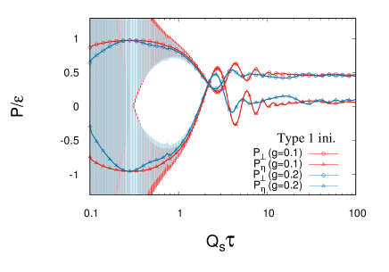
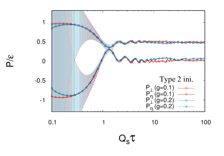
Figure 2: The time evolution of the transverse and longitudinal pressures, $P_{\perp}$ and $P_{\eta}$, per energy density $\varepsilon$ of Yang-Mills theory in the expanding geometry on the $32^{2}\times 420$ lattice, with $g=0.1$ and $0.2$; the smearing parameter $\sigma$ is set by a constraint $\sigma/g^{2}=1000$. The left and right panels show the results with the initial condition of type 1 and 2, respectively. The number of test particles is $N_{\rm TP}=96$. The lines with circles and triangles show $P_{\perp}/\varepsilon$ and $P_{\eta}/\varepsilon$, respectively.

Figure 2 shows the time evolution of the transverse and longitudinal pressures, $P_{\perp}$ and $P_{\eta}$, normalized by the energy density $\varepsilon$ at $g=0.1$ and $0.2$ for the two types of initial conditions. It is noted that error bars are large at small $Q_{s}\tau$ because large subtractions are needed. In the initial stage with $Q_{s}\tau<(1-2)$, $P_{\eta}$ is negative, which reflects that the macroscopic color electric and magnetic fields are parallel to the collision axis in the earliest stage. Then till $Q_{s}\tau<(2-3)$, $P_{\perp}$ and $P_{\eta}$ tend to come closer, and there is no $g$ dependence of their values at this period. In the later stage with $Q_{s}\tau>(2-3)$, $P_{\perp}/\varepsilon$ and $P_{\eta}/\varepsilon$ gradually approach some different constant values, respectively, with oscillatory behaviors, the amplitudes of which become tiny in the large $Q_{s}\tau$ region. The ratio $P_{\eta}/P_{\perp}$ in the final stage clearly deviates from unity; although it slightly gets closer for larger $g$ $(=0.2)$ the difference between them is still large, which means that the isotropization of the pressure is not achieved with $g\leq 0.2$. In a previous study based on the McLerran-Venugopalan model PressureEG2013 , such pressure isotropization was found at $g=0.5$ and not at $g=0.1$. Therefore, our results do not contradict their results. It is noted that the nearly constant behavior of $P_{\perp}/P_{\eta}$ at later times shown in Fig. 2 seems consistent with the kinetics results Kurkela . Such consistency may imply that the semiclassical description and the kinetic description commonly take into account one of the essential processes in the Yang-Mills theory MSkinetic ; Jkinetic .

4.2.2 Creation and growth of (Husimi-Wehrl) entropy

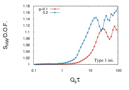
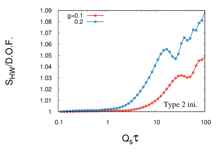
Figure 3: The time evolution of the HW entropy $S_{\rm HW}$ per degrees of freedom with the initial condition of type 1(left panel) and type 2(right panel). The other calculational conditions are the same as in Fig. 2.

In Fig. 3, we show the time evolution of $S_{\rm HW}=S_{\rm HW}^{\rm aTP}$ per degrees of freedom with $g=0.1$ and $0.2$ for the two types of initial condition. Firstly, we remark that $S_{\rm HW}$ initially agrees with unity with an error of less than 0.01%, which is in accordance with the fact that the initial conditions are prepared as a coherent state. In the earliest stage with $Q_{s}\tau<(2-3)$, the HW entropy hardly increases, and then in the intermediate stage with $Q_{s}\tau<(20-30)$, it shows a rapid growth. Then it still does show an increases on average but with smaller growth rate and an oscillatory behavior imposed. For both of the initial conditions, the larger the coupling constant, the larger the growth rate of the HW entropy. In Ref. Tsukiji2016 ; Tsukiji2018 , it was shown in the semiclassical simulation with the non-expanding geometry that in the last stage where the HW entropy production has been saturated with a small production speed, the Yang-Mills field configuration is already close to that in equilibrium. It should be noticed, however, that the similar slow production rate of the HW entropy seen in Fig. 3 does not readily mean that the system is near equilibrium since the large anisotropy of the pressure still remains in the present case with an expanding geometry, which may account for, at least partly, the slow production rate of the entropy which is actually caused by a fact that the system is still in a nonequilibrium state.

4.2.3 Relationship of particle distribution and Husimi-Wehrl entropy

To understand the underlying mechanism of the HW entropy production, we investigate the time evolution of the particle number as well as the HW entropy in piecewise with respect to different longitudinal momentum modes with an interval $|\tilde{\nu}|/\Lambda_{|\tilde{\nu}|}=0.2$, where $\Lambda_{|\tilde{\nu}|}$ denotes the ultraviolet cutoff of the momentum. Figure 4 shows the entropy increase after time evolution $\Delta S_{\rm HW}=S_{\rm HW}-N_{\rm dof}$, in several longitudinal momentum intervals with $g=0.1$ and $0.2$ for the two types of initial conditions. We find that the large HW entropy is first produced in the lowest longitudinal momentum interval, $|\tilde{\nu}|/\Lambda_{|\tilde{\nu}|}<0.2$, which is followed by an slow increase of the HW entropy in the higher longitudinal momentum intervals. Thus, the rapid production of the HW entropy shown in Fig. 3 occurs in the low longitudinal momentum modes.

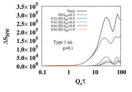
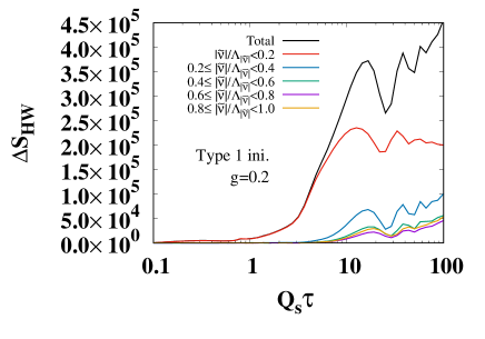
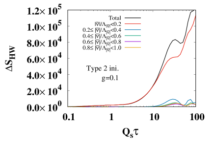
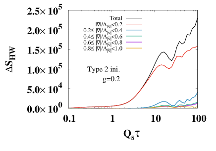
Figure 4: The HW entropy increase after time evolution, $\Delta S_{\rm HW}=S_{\rm HW}-N_{\rm dof}$, in several longitudinal momentum intervals with $g=0.1$ and $0.2$ for the two types of initial condition. The bin size in the longitudinal momentum is $|\tilde{\nu}|/\Lambda_{|\tilde{\nu}|}=0.2$. The left (right) panels show the numerical results with $g=0.1(0.2)$, and upper (lower) panels are for the type 1 (type 2) initial condition.

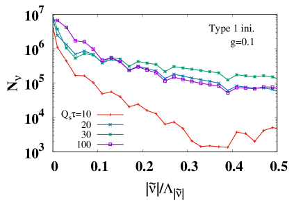
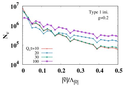
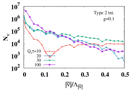
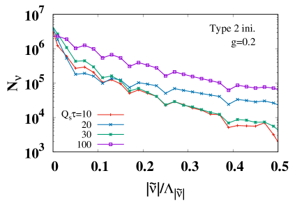
Figure 5: The time evolution of the effective particle-number distribution $N_{\nu}$ as a function of the longitudinal momentum $\tilde{\nu}$ as defined in (70) with the two initial conditions and coupling constants $g=0.1$ and $0.2$. The upper-left and upper-right panels show the numerical results for the type 1 initial condition of with $g=0.1$ and $0.2$, respectively, while that of the lower panels for the type 2 initial condition with the same $g$.

To quantify the above observation, we analyze the effective particle-numbers, since one of the proposed mechanisms of thermalization is the decay of the Yang-Mills field to particles. We define an effective particle-number $N_{\nu}$ as a function of the longitudinal momentum $\nu$ integrated over the transverse momenta as,

$$N_{\nu}\equiv \sum_{\bm{k}_{\perp},\lambda,a}\left\{\left\langle\left(\hat{a}^{a\lambda\dagger}_{\bm{k}}-\langle\hat{a}^{a\lambda\dagger}_{\bm{k}}\rangle\right)\left(\hat{a}^{a\lambda}_{\bm{k}}-\langle\hat{a}^{a\lambda}_{\bm{k}}\rangle\right)-\frac{1}{2}\right\rangle\right\}$$

$$= \sum_{\bm{k}_{\perp},\lambda,a}\left\{\left\langle\hat{a}^{a\lambda\dagger}_{\bm{k}}\hat{a}^{a\lambda}_{\bm{k}}\right\rangle-\left\langle\hat{a}^{a\lambda\dagger}_{\bm{k}}\right\rangle\left\langle\hat{a}^{a\lambda}_{\bm{k}}\right\rangle-\frac{1}{2}\right\}\ .$$ (70)

Here we regard the creation and annihilation operators subtracted with their expectation values as those operators for the particles under the background classical field. This will be a reasonable description, since the particle number is counted to be zero for a coherent state, where the HW entropy takes the minimum value. It should be noted that the last term of $-1/2$ comes from the semiclassical treatment and the uncertainty relation. In a semiclassical treatment, we cannot distinguish the order of the operators and the expectation value of the symmetrized operator (Weyl product) is observed. For example, the expectation value of the the number operator $\langle\hat{a}^{\dagger}\hat{a}\rangle$ is calculated as $\langle(\hat{a}^{\dagger}\hat{a}+\hat{a}\hat{a}^{\dagger})/2\rangle=\langle(\omega^{2}\hat{x}^{2}+\hat{p}^{2})/(2\omega)\rangle$ for a harmonic oscillator, and its minimum value is $1/2$ as long as the distribution respects the uncertainty principle. Thus the nonzero $N_{\nu}$ signals the entropy production, when we start from a coherent state initial condition.

In Fig. 5, we show the effective particle-number as a function of the longitudinal momentum $\tilde{\nu}$ at several values of $\tau$. At the initial state which is set up to be a coherent state, we find $N_{\nu}=0$ (not shown in the figure) as expected. In the earlier stage with $Q_{s}\tau=10$ (red curves), particles with the far lower longitudinal momenta dominate over those in other momentum regions. At later times, particles with higher longitudinal momenta start to increase. The early entropy production at the lower longitudinal momenta shown before thus naturally understood to be associated with the low momentum particle production.

Comparing Fig. 4 and Fig. 5, we find that the particle creation is associated with the HW entropy production, and there are two distinct stages in the evolution of fields. In the first stage, the particle number in the low longitudinal momentum region grows and the HW entropy from the low longitudinal momentum modes increases rapidly. In the second stage, the effective particle-number at higher longitudinal momenta grows and the HW entropy of higher longitudinal momentum modes increases slowly.

5 Summary

We have investigated the possible thermalization process of the highly occupied and weakly coupled Yang-Mills fields in the expanding geometry through a computation of the entropy, as given by the Husimi-Wehrl (HW) entropy, (an)isotropization of the pressure and the particle production within the semiclassical approximation: The time evolution of the system was obtained by solving the equation of motion of the Wigner function with use of the test particle method; the Husimi function is obtained by smearing the evaluated Wigner function in the phase space. The initial condition of the simulation was constructed so as to mimic the glasma initial condition MV1994_1 ; MV1994_2 ; MV1994_3 ; LMW1995_1 ; LMW1995_2 , where the macroscopic color electric and color magnetic fields are boost invariant and parallel to the collisional axis. As such, we have considered two types of initial condition whose momentum distributions are different from each other.

To obtain the HW entropy $S_{\rm HW}$ defined in terms of the Husimi function, it was first calculated by two different test particle methods, the one is called ”single test particle method (sTP)” and the other is called ”parallel test particle method (pTP)”. The resultant values thus obtained are denoted by $S_{\rm HW}^{\rm pTP}$ and $S_{\rm HW}^{\rm sTP}$, respectively, and are shown to satisfy the inequalities $S_{\rm HW}^{\rm sTP}<S_{\rm HW}<S_{\rm HW}^{\rm pTP}$. We have shown that the average value of them, $S_{\rm HW}^{\rm aTP}$, turns out to give an excellent estimate of $S_{\rm HW}$ with numerical errors of $\mathcal{O}(N_{\rm TP}^{-2})$ with $N_{\rm TP}$ being the number of test particles, $S_{\rm HW}^{\rm aTP}=S_{\rm HW}+\mathcal{O}(N_{\rm TP}^{-2})$, while $S_{\rm HW}^{\rm sTP}$ and $S_{\rm HW}^{\rm pTP}$ have numerical errors of $\mathcal{O}(N_{\rm TP}^{-1})$ , $S^{{\rm sTP}({\rm pTP})}_{\rm HW}=S_{\rm HW}+\mathcal{O}(N_{\rm TP}^{-1})$. Nevertheless, to circumvent the computational difficulty in calculating the multiple integration in the HW entropy. we have taken the product ansatz for the Wigner function.

Before proceeding with the study of the Yang-Mills field in the expanding geometry, the above computational method was checked by applying it to the massless $\phi^{4}$ scalar theory in Minkowski space-time. The numerical results in the scalar theory have indicated that $S_{\rm HW}^{\rm sTP}<S_{\rm HW}<S_{\rm HW}^{\rm pTP}$ and $S_{\rm HW}^{\rm aTP}\sim S_{\rm HW}$ nicely hold. It has been found that $S_{\rm HW}$ increases rapidly, then the growth rate becomes moderate, and finally stops increasing and keeps almost a constant value. The saturation of $S_{\rm HW}$ indicates the achievement of equilibration of the system.

We have investigated the dynamical production of the HW entropy in the semiclassical evolution of the Yang-Mills field in the expanding geometry at $g=0.1$ and $0.2$. We have also shown the semiclassical evolution of the transverse and longitudinal pressures, $P_{\perp}$ and $P_{\eta}$. Up to $Q_{s}\tau<(2-3)$, $P_{\perp}$ and $P_{\eta}$ have been found to approach each other, and there is no $g$ dependence at this time region. In the later stage with $Q_{s}\tau>(2-3)$, $P_{\perp}$ and $P_{\eta}$ have been found to approach some constant values slowly showing oscillatory behavior. The amplitude of the oscillation becomes smaller at large $Q_{s}\tau$. The longitudinal pressure relative to the transverse pressure, $P_{\eta}/P_{\perp}$, has been found to come slightly closer as $g$ increases, but a pressure isotropization was not achieved, which is not in contradiction with a previous work PressureEG2013 where a much larger coupling constant was used. After the earliest stage with $Q_{s}\tau<(2-3)$, where the HW entropy in the expanding geometry hardly increases, it grows rapidly in the following time range, $Q_{s}\tau<(20-30)$, and then increases more slowly in the later stage with $Q_{s}\tau>(20-30)$. For both types of initial conditions, the growth rate of the HW entropy at $g=0.2$ is larger than that at $g=0.1$. The slow HW entropy production stage does not readily mean that the system is near equilibrium since the large anisotropy of the pressure still remains in our simulations. Such a slow production far from equilibrium is expected to be caused by the longitudinal expansion effect.

We have defined the effective particle-number so that it represents the particle number created due to the deviations from the coherent state, and have compared its time evolution and the time evolution of the HW entropy, in piecewise of the longitudinal momentum mode. We have found that the effective particle-number and the HW entropy productions are associated with each other, and there are two distinct time stages in the time evolution of the Yang-Mills fields: In the first stage, the particle number distribution in the low longitudinal momentum region grows and the HW entropy of the longitudinal low momentum modes increases rapidly, while in the second stage, the particle number distribution at higher longitudinal momentum grows and the HW entropy of corresponding modes increases slowly.

Since our choice of the initial conditions only mimic the glasma state, we should directly take the McLerran-Venugopalan model in order to make the model more realistic MVini . It is also a rather urgent subject to perform calculations at larger coupling constant such as $g=0.5$ that is used in the previous calculation PressureEG2013 , thereby clarifying the coupling dependence of the way of the thermalization process.

Appendix A Second quantization of free gauge field in expanding geometry

In this Appendix, we present the second-quantized formulation of a free gauge field in the $\tau$-$\eta$ coordinate, which is found convenient to analyze fluctuations in the expanding glasma Berges2014_2 ; flu_EG ; Ini_flu . This appendix refers to Berges2014_2 .

First, we begin by showing the way of the second quantization in the continuum limit. In this paragraph only, all quantities are not normalized by lattice spacings. The equation of motion for the free gauge field, $[D,F]=0$, describing the $\tau$ evolution reads

$$\partial_{1}\partial_{\tau}A_{1}(x)+\partial_{2}\partial_{\tau}A_{2}(x)+\frac{1}{\tau^{2}}\partial_{\eta}\partial_{\tau}A_{\eta}(x)=0\ ,$$ (71)

$$\left(\partial^{2}_{\tau}+\frac{1}{\tau}\partial_{\tau}-\partial^{2}_{1}-\partial^{2}_{2}-\frac{\partial^{2}_{\eta}}{\tau^{2}}\right)A_{i}(x)+\partial_{i}\left(\partial_{1}A_{1}(x)+\partial_{2}A_{2}(x)+\frac{1}{\tau^{2}}\partial_{\eta}A_{\eta}(X)\right)=0\ ,$$ (72)

$$\left(\partial^{2}_{\tau}-\frac{1}{\tau}\partial_{\tau}-\partial^{2}_{1}-\partial^{2}_{2}-\frac{\partial^{2}_{\eta}}{\tau^{2}}\right)A_{\eta}(x)+\partial_{\eta}\left(\partial_{1}A_{1}(x)+\partial_{2}A_{2}(x)+\frac{1}{\tau^{2}}\partial_{\eta}A_{\eta}(X)\right)=0.$$ (73)

For the Fourier modes with finite transverse momentum mode, the general solution satisfying the Coulomb type gauge condition, $\left(\partial_{1}A_{1}+\partial_{2}A_{2}+\tau^{-2}\partial_{\eta}A_{\eta}\right)\Bigl{|}_{\tau=\tau_{0}}=0$, is expressed in terms of the Hankel function,

$$A_{\mu}=\sum_{\lambda=1,2}\int\frac{d^{3}\bm{k}}{(2\pi)^{3}}\left(\xi^{\lambda,(1)}_{\bm{k}}\mathcal{A}^{(-)\lambda}_{\mu,\bm{k}}(\tau)e^{i(\bm{k}_{\perp}\cdot\bm{x}_{\perp}+\nu\eta)}+\xi^{\lambda,(2)}_{\bm{k}}\mathcal{A}^{(+)\lambda}_{\mu,\bm{k}}(\tau)e^{i(\bm{k}_{\perp}\cdot\bm{x}_{\perp}+\nu\eta)}\right)\ ,$$ (74)

$$\mathcal{A}^{(^{-}/_{+})1}_{\mu,\bm{k}}(\tau)=\frac{i}{k_{\perp}}(0,k_{2},-k_{1},0)H^{(^{1}/_{2})}_{i\nu}(k_{\perp}\tau)\ ,$$ (75)

$$\mathcal{A}^{(^{-}/_{+})2}_{\mu,\bm{k}}(\tau)=-\frac{\nu}{k_{\perp}}\left(0,k_{1}\alpha^{(^{1}/_{2})}_{i\nu}(k_{\perp}\tau),k_{2}\alpha^{(^{1}/_{2})}_{i\nu}(k_{\perp}\tau),-\frac{1}{\nu}\beta^{(^{1}/_{2})}_{i\nu}(k_{\perp}\tau)\right)\ ,$$ (76)

$$\alpha^{(^{1}/_{2})}_{i\nu}(k_{\perp}\tau)=\int^{k_{\perp}\tau}_{k_{\perp}\tau_{0}}dz\frac{1}{z}H^{(^{1}/_{2})}_{i\nu}(z)-\frac{k_{\perp}\tau_{0}}{\nu^{2}+(k_{\perp}\tau_{0})^{2}}\dot{H}^{(^{1}/_{2})}_{i\nu}(k_{\perp}\tau_{0})\ ,$$ (77)

$$\beta^{(^{1}/_{2})}_{i\nu}(k_{\perp}\tau)=\int^{k_{\perp}\tau}_{k_{\perp}\tau_{0}}dzzH^{(^{1}/_{2})}_{i\nu}(z)-\frac{(k_{\perp}\tau_{0})^{3}}{\nu^{2}+(k_{\perp}\tau_{0})^{2}}\dot{H}^{(^{1}/_{2})}_{i\nu}(k_{\perp}\tau_{0})\ ,$$ (78)

where $k_{\perp}=\sqrt{k^{2}_{1}+k^{2}_{2}}$ is a transverse momentum and $\xi^{\lambda,i}_{\bm{k}}$ is a given constant. The solution, $\mathcal{A}^{(i)\lambda}_{\mu,\bm{k}}(\tau)e^{i(\bm{k}_{\perp}\cdot\bm{x}_{\perp}+\nu\eta)}$, is orthogonal to other solution having different indexes $(\lambda^{\prime},i^{\prime},\bm{k}^{\prime})\neq(\lambda,i,\bm{k})$,

$$\left(\mathcal{A}^{(i)\lambda}_{\mu,\bm{k}}(\tau)e^{i\bm{k}\cdot\bm{x}},\mathcal{A}^{(i^{\prime})\lambda}_{\mu^{\prime},\bm{k}^{\prime}}(\tau)e^{i\bm{k}^{\prime}\cdot\bm{x}}\right)=0\ ,$$ (79)

with respect to a scalar product defined as

$$\left(f_{\mu}(x),g_{\mu}(x)\right)=-i\int d^{3}\bm{x}\tau g^{\mu\nu}\left(f^{*}_{\mu}(x)\partial_{\tau}g_{\nu}(x)-g_{\nu}(x)\partial_{\tau}f^{*}_{\mu}(x)\right)\ .$$ (80)

If $(\lambda^{\prime},i^{\prime},\bm{k}^{\prime})=(\lambda,i,\bm{k})$, the scalar product is not vanished and is invariant under the $\tau$ evolution according to Eq. (71)-(73). Since the second kind of Hankel function asymptotically behaves as the positive frequency mode,

$$H^{(i)}_{i\nu}(k_{\perp}\tau)\to\sqrt{\frac{2}{\pi k_{\perp}\tau}}\exp{\left[-i\left(k_{\perp}\tau-\frac{\pi}{4}\right)-\frac{\pi\nu}{2}\right]}\ \ \ (k_{\perp}\tau\rightarrow\infty)\ ,$$ (81)

we can obtain the expression of the second-quantized gauge field as the linear combination of $\mathcal{A}^{(+)1}_{\mu}(\tau,\bm{k})$ and $\mathcal{A}^{(+)2}_{\mu}(\tau,\bm{k})$,

$$A_{i}(x)=\sum_{\lambda}\int\frac{d^{3}\bm{k}}{(2\pi)^{3}}\left(\hat{a}^{\lambda}_{\bm{k}}\mathcal{A}^{\lambda}_{\mu,\bm{k}}(\tau)e^{i(\bm{k}_{\perp}\cdot\bm{x}_{\perp}+\nu\eta)}+{\rm h.c.}\right)\ ,$$ (82)

$$\mathcal{A}^{\lambda}_{\mu,\bm{k}}(\tau)=\sqrt{\frac{\pi}{4}}e^{\frac{\pi|\nu|}{2}}\mathcal{A}^{(+)\lambda}_{\mu,\bm{k}}(\tau)\ ,$$ (83)

$$\left[\hat{a}^{\lambda}_{\bm{k}},\hat{a}^{\lambda^{\prime}\dagger}_{\bm{k}^{\prime}}\right]=(2\pi)^{3}\delta_{\lambda,\lambda^{\prime}}\delta(\bm{k}-\bm{k}^{\prime})\ .$$ (84)

Here we determine the normalization constant in front of $\mathcal{A}^{(+)\lambda}_{\mu,\bm{k}}(\tau)$ in Eq. (83) so as to satisfy the ortho-normal condition,

$$\left(\sqrt{\frac{\pi}{4}}e^{\frac{\pi|\nu|}{2}}\mathcal{A}^{(+)\lambda}_{\mu,\bm{k}}(\tau)e^{i(\bm{k}_{\perp}\cdot\bm{x}_{\perp}+\nu\eta)},\sqrt{\frac{\pi}{4}}e^{\frac{\pi|\nu^{\prime}|}{2}}\mathcal{A}^{(+)\lambda^{\prime}}_{\mu,\bm{k}^{\prime}_{\perp},\nu^{\prime}}(\tau)e^{i(\bm{k}^{\prime}_{\perp}\cdot\bm{x}_{\perp}+\nu^{\prime}\eta)}\right)$$

$$=(2\pi)^{3}\delta_{\lambda,\lambda^{\prime}}\delta(\bm{k}_{\perp}-\bm{k}^{\prime}_{\perp})\delta(\nu-\nu^{\prime})\ ,$$ (85)

The procedure of the second quantization using such a scalar product is standard in Quantum field theory in curved space-time. In our analysis, we only treat the finite transverse momentum modes since the contribution of the $0$ transverse mode decreases as the transverse size of the system becomes large.

Next, we show the second quantization of the free gauge field on the space lattice with the continuous time. The equation of motion reads

$$\partial^{\rm B}_{1}\partial_{\tau}A_{1}(x)+\partial^{\rm B}_{2}\partial_{\tau}A_{2}(x)+\frac{1}{a^{2}_{\eta}\tau^{2}}\partial^{\rm B}_{\eta}\partial_{\tau}A_{\eta}(x)=0\ ,$$ (86)

$$\left(\partial^{2}_{\tau}+\frac{1}{\tau}\partial_{\tau}-\partial^{\rm B}_{1}\partial^{\rm F}_{1}-\partial^{\rm B}_{2}\partial^{\rm F}_{2}-\frac{\partial^{\rm B}_{\eta}\partial^{\rm F}_{\eta}}{a^{2}_{\eta}\tau^{2}}\right)A_{i}(x)$$

$$\ \ \ \ \ \ \ \ \ \ +\partial_{i}\left(\partial^{\rm B}_{1}A_{1}(x)+\partial^{\rm B}_{2}A_{2}(x)+\frac{1}{a^{2}_{\eta}\tau^{2}}\partial^{\rm B}_{\eta}A_{\eta}(X)\right)=0\ ,$$ (87)

$$\left(\partial^{2}_{\tau}-\frac{1}{\tau}\partial_{\tau}-\partial^{\rm B}_{1}\partial^{\rm F}_{1}-\partial^{\rm B}_{2}\partial^{\rm F}_{2}-\frac{\partial^{\rm B}_{\eta}\partial^{\rm F}_{\eta}}{a^{2}_{\eta}\tau^{2}}\right)A_{\eta}(x)$$

$$\ \ \ \ \ \ \ \ \ \ +\partial_{i}\left(\partial^{\rm B}_{1}A_{1}(x)+\partial^{\rm B}_{2}A_{2}(x)+\frac{1}{a^{2}_{\eta}\tau^{2}}\partial^{\rm B}_{\eta}A_{\eta}(X)\right)=0\ ,$$ (88)

where $\partial^{\rm B}_{i}$ denotes a backward difference operator in the $i$-direction. In much the same way as the continuum case, we can get the expression of the second-quantized gauge field as

$$A_{i}(x)=\frac{1}{\sqrt{L^{2}_{\perp}L_{\eta}}}\sum_{\lambda,\bm{k}}\left(\hat{a}^{\lambda}_{\bm{k}}\tilde{\mathcal{A}}^{\lambda}_{\mu,\bm{k}}(\tau)e^{i(\bm{k}_{\perp}\cdot\bm{x}_{\perp}+\nu\eta)}+{\rm h.c.}\right)\ ,$$ (89)

$$\left[\hat{a}^{\lambda}_{\bm{k}},\hat{a}^{\lambda^{\prime}\dagger}_{\bm{k}}\right]=\delta_{\lambda,\lambda^{\prime}}\delta_{\bm{k},\bm{k}^{\prime}}\ ,$$ (90)

$$\tilde{\mathcal{A}}^{1}_{\mu,\bm{k}}(\tau)=\frac{i}{\omega_{\bm{k}_{\perp}}}\sqrt{\frac{\pi}{4a_{\eta}}}e^{\frac{\pi|\tilde{\nu}|}{2a_{\eta}}}(0,\tilde{k}_{2},\tilde{k}_{1},0)H^{(2)}_{i|\tilde{\nu}|/a_{\eta}}(\omega_{\bm{k}_{\perp}}\tau)\ ,$$ (91)

$$\tilde{\mathcal{A}}^{2}_{\mu,\bm{k}}(\tau)=-\frac{\tilde{\nu}^{*}}{a_{\eta}\omega_{\bm{k}_{\perp}}}\sqrt{\frac{\pi}{4a_{\eta}}}e^{\frac{\pi|\tilde{\nu}|}{2a_{\eta}}}\left(0,\tilde{k}_{1}\alpha^{(2)}_{i|\tilde{\nu}|/a_{\eta}}(\omega_{\bm{k}_{\perp}}\tau),\tilde{k}_{2}\alpha^{(2)}_{i|\tilde{\nu}|/a_{\eta}}(\omega_{\bm{k}_{\perp}}\tau),-\frac{a_{\eta}^{2}}{\tilde{\nu}^{*}}\beta^{(2)}_{i|\tilde{\nu}|/a_{\eta}}(\omega_{\bm{k}_{\perp}}\tau)\right)\ .$$ (92)

By utilizing this expression, the electric field and the free part of the magnetic field are also written in terms of the annihilation and creation operators,

$$\hat{E}^{i}(x)=\frac{1}{\sqrt{L^{2}_{\perp}L_{\eta}}}\sum_{\lambda,\bm{k}}\left(\hat{a}^{\lambda}_{\bm{k}}\mathcal{E}^{\lambda,i}_{\bm{k}}(\tau)e^{i(\bm{k}_{\perp}\cdot\bm{x}_{\perp}+\nu\eta)}+{\rm h.c.}\right)\ ,$$ (93)

$$\hat{B}^{i}_{0}(x)=\frac{1}{2}\epsilon^{ijk}\partial^{\rm F}_{j}A_{k}(x)=\frac{1}{\sqrt{L^{2}_{\perp}L_{\eta}}}\sum_{\lambda,\bm{k}}\left(\hat{a}^{\lambda}_{\bm{k}}\mathcal{B}^{\lambda,i}_{\bm{k}}(\tau)e^{i(\bm{k}_{\perp}\cdot\bm{x}_{\perp}+\nu\eta)}+{\rm h.c.}\right)\ ,$$ (94)

$$\mathcal{E}^{1,i}_{\bm{k}}(\tau)=\dot{H}^{(2)}_{i|\tilde{\nu}|/a_{\eta}}(\omega_{\bm{k}_{\perp}}\tau)\varepsilon^{1,i}_{\bm{k}}\ ,\ \ \mathcal{E}^{2,i}_{\bm{k}}(\tau)=H^{(2)}_{i|\tilde{\nu}|/a_{\eta}}(\omega_{\bm{k}_{\perp}}\tau)\varepsilon^{2,i}_{\bm{k}}\ ,$$ (95)

$$\mathcal{B}^{1,i}_{\bm{k}}(\tau)=H^{(2)}_{i|\tilde{\nu}|/a_{\eta}}(\omega_{\bm{k}_{\perp}}\tau)\varepsilon^{2,i*}_{\bm{k}}\ ,\ \ \mathcal{B}^{2,i}_{\bm{k}}(\tau)=\dot{H}^{(2)}_{i|\tilde{\nu}|/a_{\eta}}(\omega_{\bm{k}_{\perp}}\tau)\varepsilon^{1,i*}_{\bm{k}}\ ,$$ (96)

$$\varepsilon^{1,i}_{\bm{k}}=ia_{\eta}\tau\sqrt{\frac{\pi}{4a_{\eta}}}e^{\frac{\pi|\tilde{\nu}|}{2a_{\eta}}}(\tilde{k}^{*}_{2},-\tilde{k}^{*}_{1},0)\ ,\ \ \varepsilon^{2,i}_{\bm{k}}=-\frac{\tilde{\nu}^{*}}{\omega_{\bm{k}_{\perp}}}\sqrt{\frac{\pi}{4a_{\eta}}}e^{\frac{\pi|\tilde{\nu}|}{2a_{\eta}}}\left(\tilde{k}_{1},\tilde{k}_{2},-\frac{\omega^{2}_{\bm{k}_{\perp}}}{\tilde{\nu}^{*}}\right)\ .$$ (97)

Solving Eq. (93) and Eq. (94) with respect to $\hat{a}^{\lambda}_{\bm{k}}$, we can write $\hat{a}^{\lambda}_{\bm{k}}$ as the linear combination of the Fourier modes, $(\hat{E}_{\bm{k}},\hat{B}_{\bm{k}})$,

$$\hat{a}^{1}_{\bm{k}} =\frac{i}{a_{\eta}\omega_{\bm{k}_{\perp}}\tau}$$

$$\times\left(\frac{\omega^{2}_{\bm{k}_{\perp}}}{\omega^{2}_{\bm{k}_{\perp}}+|\tilde{\nu}/(\tau a_{\eta})|^{2}}\frac{\dot{H}^{(2)*}_{i|\tilde{\nu}|/a_{\eta}}(\omega_{\bm{k}_{\perp}}\tau)}{H^{(2)*}_{i|\tilde{\nu}|/a_{\eta}}(\omega_{\bm{k}_{\perp}}\tau)}\left[\mathcal{B}^{1*}_{\bm{k}}\cdot B_{0,\bm{k}}(\tau)\right]+\frac{H^{(2)*}_{i|\tilde{\nu}|/a_{\eta}}(\omega_{\bm{k}_{\perp}}\tau)}{\dot{H}^{(2)*}_{i|\tilde{\nu}|/a_{\eta}}(\omega_{\bm{k}_{\perp}}\tau)}\left[\mathcal{E}^{1,*}_{\bm{k}}\cdot E_{\bm{k}}(\tau)\right]\right)\ ,$$ (98)

$$\hat{a}^{2}_{\bm{k}} =\frac{i}{a_{\eta}\omega_{\bm{k}_{\perp}}\tau}$$

$$\times\left(\frac{\omega^{2}_{\bm{k}_{\perp}}}{\omega^{2}_{\bm{k}_{\perp}}+|\tilde{\nu}/(\tau a_{\eta})|^{2}}\frac{\dot{H}^{(2)*}_{i|\tilde{\nu}|/a_{\eta}}(\omega_{\bm{k}_{\perp}}\tau)}{H^{(2)*}_{i|\tilde{\nu}|/a_{\eta}}(\omega_{\bm{k}_{\perp}}\tau)}\left[\mathcal{E}^{2*}_{\bm{k}}\cdot E_{\bm{k}}(\tau)\right]+\frac{H^{(2)*}_{i|\tilde{\nu}|/a_{\eta}}(\omega_{\bm{k}_{\perp}}\tau)}{\dot{H}^{(2)*}_{i|\tilde{\nu}|/a_{\eta}}(\omega_{\bm{k}_{\perp}}\tau)}\left[\mathcal{B}^{2*}_{\bm{k}}\cdot B_{0,\bm{k}}(\tau)\right]\right)\ .$$ (99)

In actual calculations, we use these relations to transform $(A,E)$ to $(\Phi,\Pi)$ through Eq. (54) and Eq. (55).

Appendix B Divergence in pressure and energy density

In this appendix, we show the remaining divergences in the pressure and energy density after subtracting the vacuum contribution, and discuss how to subtract them. For convenience, we use the following notation $()_{\rm ini\ mac}$, which means the contribution of macroscopic field part of the initial Wigner function to a given observable at the initial time $\tau_{0}$. For example, in the case of the Fourier transforms of the color electric and color magnetic fields, $(\bm{E}^{a}_{\bm{k}})_{\rm ini\ mac}$ and $(\bm{B}^{a}_{\bm{k}})_{\rm ini\ mac}$ have been already given in Eq. (59)-(64). Thus, the the macroscopic field contribution to the initial pressure are given by

$$(P_{\eta})_{\rm ini\ mac}\sim-(P_{\perp})_{\rm ini\ mac} =-\frac{1}{V}\sum_{x}g_{ii}\left(\hat{T}^{ii}(x)\right)_{\rm ini\ mac}$$

$$=-\frac{a_{\eta}\tau}{2}\sum_{a,\bm{x}_{\perp},\eta}\left[\left(\hat{E}^{a\eta}(x)^{2}\right)_{\rm ini\ mac}+\left(\hat{B}^{a\eta}(x)^{2}\right)_{\rm ini\ mac}\right]$$

$$\sim-\frac{\Delta}{8L^{2}_{\perp}\alpha_{s}}\sum_{\bm{k}_{\perp}}\omega^{2}_{\bm{k}_{\perp}}|f_{l}(\bm{k}_{\perp})|^{2}\ .$$ (100)

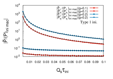
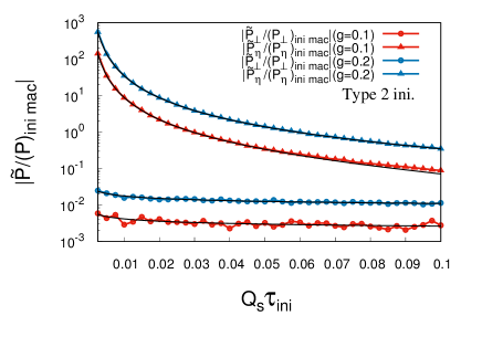
Figure 6: The $Q_{s}\tau_{0}$ dependence of the initial pressure after subtracting the vacuum contribution and the macroscopic field contribution, $\tilde{P}_{i}=\frac{1}{V}\sum_{x}g_{ii}\left\langle\hat{T}^{ii}(x)\right\rangle_{\rm mat+flu}-\frac{1}{V}\sum_{x}g_{ii}\left\langle\hat{T}^{ii}(x)\right\rangle_{\rm vac}-(P_{i})_{\rm ini\ mac}$, normalized by $(P_{i})_{\rm ini\ mac}$. These calculations are performed at at $g=0.1$ and $0.2$ for two types of initial condition. The red (blue) line with circles shows the transverse pressure at $g=0.1$ $(0.2)$. The red (blue) line with triangular points shows longitudinal one at $g=0.1$ $(0.2)$. The result in the left (right) panel is calculated with the type $1$ ($2$) initial condition.

In Fig. 6, we show the $Q_{s}\tau_{0}$ dependence of the initial pressure after subtracting the vacuum contribution and the macroscopic field contribution,

$$\tilde{P}_{i}=\frac{1}{V}\sum_{x}g_{ii}\left\langle\hat{T}^{ii}(x)\right\rangle_{\rm mat+flu}-\frac{1}{V}\sum_{x}g_{ii}\left\langle\hat{T}^{ii}(x)\right\rangle_{\rm vac}-(P_{i})_{\rm ini\ mac}\ ,$$ (101)

normalized by $(P_{i})_{\rm ini\ mac}$ at $g=0.1$ and $0.2$ for two types of initial condition. We find that $\left|\tilde{P}_{\eta}/(P_{\eta})_{\rm ini\ mac}\right|$ diverges as $(Q_{s}\tau_{0})^{-2}$ since the $Q_{s}\tau_{0}$ dependence of $\left|\tilde{P}_{\eta}/(P_{\eta})_{\rm ini\ mac}\right|$ is reproduced well by the fitting function $f_{\rm pow}(Q_{s}\tau_{0})=A_{\rm pow}/(Q_{s}\tau_{0})^{2}$. We also find that $\left|\tilde{P}_{\perp}/(P_{\perp})_{\rm ini\ mac}\right|$ diverges as $\ln^{2}{Q_{s}\tau_{0}}$ since $\left|\tilde{P}_{\perp}/(P_{\perp})_{\rm ini\ mac}\right|$ data lie on the fitting curve $f_{\rm log}(Q_{s}\tau_{0})=B_{\rm log}\ln^{2}{(Q_{s}\tau_{0})}+C_{\rm log}$.

Here, we briefly explain how to remove the remaining divergence at any $\tau$ based on the method presented in Ref. PressureEG2013 . As seen above, the remaining divergence in $P_{\perp}$ at $\tau=\tau_{0}$ is a logarithmic function of $\tau_{0}$ and is much smaller than the initial macroscopic field contribution,

$$B_{\rm log}\ln^{2}{(Q_{s}\tau_{0})}\gg|(P_{\perp})_{\rm ini\ mac}|\ .$$ (102)

Thus, we assume to neglect the remaining divergence in $P_{\perp}$ at any $\tau$. Then we can define the subtracted energy density and pressure as

$$\varepsilon\equiv\frac{1}{V}\sum_{x}g_{\tau\tau}\left\langle\hat{T}^{\tau\tau}(x)\right\rangle_{\rm mac+fluc}-\frac{1}{V}\sum_{x}g_{\tau\tau}\left\langle\hat{T}^{\tau\tau}(x)\right\rangle_{\rm vac}-\alpha_{\rm div}(t)\ ,$$ (103)

$$P_{i}\equiv\frac{1}{V}\sum_{x}g_{ii}\left\langle\hat{T}^{ii}(x)\right\rangle_{\rm mac+fluc}-\frac{1}{V}\sum_{x}g_{ii}\left\langle\hat{T}^{ii}(x)\right\rangle_{\rm vac}-\delta_{i,\eta}\alpha_{\rm div}(t)\ ,$$ (104)

where $\alpha_{\rm div}(\tau)$ represents the divergence that should be removed. The energy density also has the remaining divergence because of the relation between the energy density and pressure, $\varepsilon=P_{1}+P_{2}+P_{\eta}$. By using the conservation law in the boost invariant longitudinal (Bjorken) expanding geometry, $\partial\varepsilon/\partial\tau=-\varepsilon+P_{\eta}/\tau$, we obtain the evolution equation for $\alpha$,

$$\frac{d\alpha_{\rm div}}{d\tau}=-\frac{2\alpha_{\rm div}}{\tau}\ .$$ (105)

By solving the differential equation, we find $\alpha_{\rm div}(\tau)=\alpha/\tau^{2}$, where $\alpha$ is a constant. As seen above, we can obtain $\alpha(\tau_{0})$ as $\alpha(\tau_{0})=A_{\rm pow}/(Q_{s}\tau_{0})^{2}$ by the fit. Thus, we use $\alpha=A_{\rm pow}$ in actual calculations.

Appendix C Evaluation by test particle methods

An integral $I$ consisting of a function $H(\Gamma)$ that is evaluated by test particle methods is expressed as

$$I=\int{\rm d}\Gamma{\cal F}(H(\Gamma)),$$ (106)

where $\Gamma$ denotes the phase space point under consideration. In general, $H(\Gamma)$ evaluated with $i$-th set of test particles, which is represented as $H_{i}(\Gamma)$, has numerical errors $dH_{i}(\Gamma)$ depending on the phase space point $\Gamma$ as

$$H_{i}(\Gamma)=H(\Gamma)+dH_{i}(\Gamma).$$ (107)

Note that each $H(\Gamma)$ that enters the integral $I$ can be evaluated with different and independent sets of test particles. (When all the test particle sets are identical, it is called the single test particle method.) Then, under the condition $\frac{dH}{H}\ll 1$, the integral $I$ can be expanded as a series of $dH_{i}(\Gamma)$,

$$I=\int{\rm d}\Gamma{\cal F}(H)+\sum_{i1,i2,..,iN}\int{\rm d}\Gamma{\cal F^{\prime}}^{1,2,..,N}_{i1,i2,..,iN}dH_{1}^{i1}dH_{2}^{i2}..dH_{N}^{iN},$$ (108)

where ${\cal F^{\prime}}$ denotes coefficients in the expansion, and $\Gamma$ in the functions are omitted. We here consider the situation where the integrals of the odd-order terms of $dH$ disappear due to numerical error cancellation as $\int{\rm d}\Gamma dH_{i}^{2n+1}(\Gamma){\cal G}(\Gamma)=0$, which would be justified when positive and negative contributions of $dH_{i}(\Gamma)$ equally enter in the integration as $\int{\rm d}\Gamma dH_{i}(\Gamma)=0$ and ${\cal G}$ is smooth enough. In such a case, only even-order terms contribute to $I$’s numerical errors as

$$I=\int{\rm d}\Gamma{\cal F}(H)+\sum_{i1,i2,..,iN\in{\rm even}}\int{\rm d}\Gamma{\cal F^{\prime}}^{1,2,..,N}_{i1,i2,..,iN}dH_{1}^{i1}dH_{2}^{i2}..dH_{N}^{iN},$$ (109)

and the number of terms is greatly reduced.

Let us proceed with the evaluation of a HW entropy based on test particle methods. A HW-entropy $S$ can be expressed as

$$S=-\int d\Gamma H(\Gamma)\ln H(\Gamma),$$ (110)

with a Husimi function $H(\Gamma)$. With the parallel test particle (pTP) method in mind, $S$ can be written as

$$S = -\int d\Gamma H_{1}(\Gamma)\ln H_{2}(\Gamma)$$ (111)

$$= -\int d\Gamma(H(\Gamma)+dH_{1}(\Gamma))\ln(H(\Gamma)+dH_{2}(\Gamma))\ ,$$

which is further expanded as

$$S=-\int{\rm d}\Gamma H(\Gamma)\ln H(\Gamma)-\int{\rm d}\Gamma dH_{1}(\Gamma)\ln H(\Gamma)-\int{\rm d}\Gamma dH_{2}(\Gamma)$$

$$-\int{\rm d}\Gamma\frac{dH_{1}(\Gamma)dH_{2}(\Gamma)}{H(\Gamma)}+\int{\rm d}\Gamma\frac{dH_{2}^{2}(\Gamma)}{2H(\Gamma)}+\int{\rm d}\Gamma\frac{dH_{1}(\Gamma)dH_{2}^{2}(\Gamma)}{2H(\Gamma)}+\cdots\ ,$$ (112)

when $\frac{dH}{H}\ll 1$. In the case where $H(\Gamma)$ is a Husimi function, we have confirmed the equality $\int{\rm d}\Gamma H(\Gamma)=1$ numerically holds in a good accuracy, which indicates that positive and negative contributions of $dH_{i}(\Gamma)$ equally enter in the integration, and the integrals of the odd-order terms of $dH$ is expected to disappear due to numerical error cancellation as $\int{\rm d}\Gamma dH^{2n+1}(\Gamma){\cal G}(\Gamma)=0$, since ${\cal G}(\Gamma)$ is a function of $H(\Gamma)$, which is a smooth Gaussian-smeared function. Such error cancellation has been numerically confirmed at least in the calculations presented in this paper, and we can leave only even-order terms of $dH$.

For the single test particle (sTP) method, the errors in and outside the logarithmic function are identical ($dH_{1}=dH_{2}$) and $S$ leads to the form,

$$S^{\rm sTP}=-\int{\rm d}\Gamma H(\Gamma)\ln H(\Gamma)-\int{\rm d}\Gamma\frac{dH_{2}^{2}(\Gamma)}{2H(\Gamma)}\ .$$ (113)

For the parallel test particle (pTP) method, $dH_{1}$ and $dH_{2}$ are independent, and

$$S^{\rm pTP}=-\int{\rm d}\Gamma H(\Gamma)\ln H(\Gamma)+\int{\rm d}\Gamma\frac{dH_{2}^{2}(\Gamma)}{2H(\Gamma)}$$ (114)

holds. We finally obtain the inequality,

$$S^{\rm sTP}<S<S^{\rm pTP}.$$ (115)

When the test particles used for evaluating $\ln H(\Gamma)$ are common in sTP and pTP methods, the entropy evaluated with $N_{\rm TP}\rightarrow\infty$ can be obtained as

$$S=\frac{S^{\rm sTP}+S^{\rm pTP}}{2}+\mathcal{O}(N_{\rm TP}^{-2}),$$ (116)

where we make the reasonable assumption, $dH\propto 1/\sqrt{N_{\rm TP}}$.

Appendix D Choice of the smearing parameter

Here we show how the HW entropy defined in Eq. (20), in which the smear parameters are set to the eigenfrequencies, behaves for the Gibbs state and vacuum state of the free field.

We first discuss the HW entropy defined in Eq. (20) for the Gibbs ensemble of the free field, $\rho^{\rm free}_{\rm Gibbs}\propto e^{-H_{\rm free}/T}$. In this case, the total density matrix, $\rho^{\rm free}_{\rm Gibbs}$, can be written as the product of the Gibbs ensembles of one-dimensional harmonic oscillators, $\rho^{\rm free}_{\rm Gibbs}=\prod_{\bm{k}}\rho^{\rm h.o.}_{{\rm Gibbs},\bm{k}}\propto\prod_{\bm{k}}e^{-H^{\rm h.o.}_{\bm{k}}/T}$. Then the total Husimi function can also be written as the product of the Husimi functions for each degree of freedom,

$$f_{\rm H}(\{\Phi,\Pi,\omega\})\Big{|}_{\rho=\rho^{\rm free}_{\rm Gibbs}}=\prod_{\bm{k}}f_{\rm H}(\Phi_{\bm{k}},\Pi_{\bm{k}},\omega_{\bm{k}})\Big{|}_{\rho=\rho^{\rm h.o.}_{{\rm Gibbs},\bm{k}}}\ .$$ (117)

Therefore, the total HW entropy, $S_{\rm HW}|_{\rho=\rho^{\rm free}_{\rm Gibbs}}$, is given by the sum of the HW entropy for each degree of freedom,

$$S_{\rm HW}(\{\omega\})\Big{|}_{\rho=\rho^{\rm free}_{\rm Gibbs}} =-\int\mathcal{D}\Gamma f_{\rm H}(\{\Phi,\Pi,\omega\})\ln{f_{\rm H}(\{\Phi,\Pi,\omega\})}\Big{|}_{\rho=\rho^{\rm free}_{\rm Gibbs}}$$

$$=\sum_{\bm{k}}-\int\frac{d\Phi_{\bm{k}}d\Pi_{\bm{k}}}{2\pi}f_{\rm H}(\Phi_{\bm{k}},\Pi_{\bm{k}},\omega_{\bm{k}})\ln{f_{\rm H}(\Phi_{\bm{k}},\Pi_{\bm{k}},\omega_{\bm{k}})}\Big{|}_{\rho=\rho^{\rm h.o.}_{{\rm Gibbs},\bm{k}}}$$

$$=\sum_{\bm{k}}S_{\rm HW}(\omega_{\bm{k}})\Big{|}_{\rho=\rho^{\rm h.o.}_{{\rm Gibbs},\bm{k}}}\ .$$ (118)

On the basis of the discussion of the HW entropy of an one-dimensional harmonic oscillator with the smearing parameter being set to its eigenfrequency, which is given in Sec. $5$ in Ref. Kyoto2009 , the HW entropy for each degree of freedom, $S_{\rm HW}(\omega_{\bm{k}})\Big{|}_{\rho=\rho^{\rm h.o.}_{{\rm Gibbs},\bm{k}}}$, is found to be larger than the von-Neumann entropy $S_{\rm vN}\left(=-{\rm Tr}(\rho^{\rm h.o.}_{{\rm Gibbs},\bm{k}}\ln\rho^{\rm h.o.}_{{\rm Gibbs},\bm{k}})\right)$ obtained from the same density matrix, but to agree with it in the high-temperature limit,

$$S_{\rm HW}(\omega_{\bm{k}})\Big{|}_{\rho=\rho^{\rm h.o.}_{{\rm Gibbs},\bm{k}}} >S_{\rm vN}\Big{|}_{\rho=\rho^{\rm h.o.}_{{\rm Gibbs},\bm{k}}}\ ,$$ (119)

$$\lim_{T\to\infty}S_{\rm HW}(\omega_{\bm{k}})\Big{|}_{\rho=\rho^{\rm h.o.}_{{\rm Gibbs},\bm{k}}} =\lim_{T\to\infty}S_{\rm vN}\Big{|}_{\rho=\rho^{\rm h.o.}_{{\rm Gibbs},\bm{k}}}\ .$$ (120)

Accordingly. the same relationship holds for for the total HW entropy and the von-Neumann entropy given as a sum of harmonic oscillators,

$$S_{\rm HW}(\{\omega\})\Big{|}_{\rho=\rho^{\rm free}_{\bm{k}}} >S_{\rm vN}\Big{|}_{\rho=\rho^{\rm free}_{\bm{k}}}\ ,$$ (121)

$$\lim_{T\to\infty}S_{\rm HW}(\{\omega\})\Big{|}_{\rho=\rho^{\rm free}_{\bm{k}}} =\lim_{T\to\infty}S_{\rm vN}\Big{|}_{\rho=\rho^{\rm free}_{\bm{k}}}\ ,$$ (122)

where $S_{\rm vN}\Big{|}_{\rho=\rho^{\rm free}_{\bm{k}}}=\sum_{\bm{k}}S_{\rm vN}\Big{|}_{\rho=\rho^{\rm h.o.}_{{\rm Gibbs},\bm{k}}}$. This shows that the HW entropy $S_{\rm HW}(\{\omega_{\bm{k}}\})$ adopted in our study agrees with the von-Neumann entropy in the high-temperature and weak-coupling limit.

Next, we show that the HW entropy defined by Eq. (20) takes the minimum value 1 for the perturbative vacuum state as

$$S_{\rm HW}(\{\omega\})\geq S_{\rm HW}(\{\omega\})\Big{|}_{|0\rangle\langle 0|}=1.$$ (123)

To show the above inequality, we utilize the theorem given in Refs. Lieb1978 ; Carlen1990 stating that, in general, the HW entropy for given conjugate variables $(\hat{x},\hat{p})$ and smearing parameter $\sigma$ takes the minimum value $1$ for the coherent state $|\alpha;\sigma\rangle$ defined as the eigenstate of the ”annihilation operator”, $\hat{a}=(\sigma\hat{x}+i\hat{p})/\sqrt{2\sigma}$:

$$S_{\rm HW}(\sigma)\geq S_{\rm HW}(\sigma)\Big{|}_{|\alpha;\sigma\rangle\langle\alpha;\sigma|}=1.$$ (124)

Then, one sees that the HW entropy with the smearing width $\{\omega_{\bm{k}}\}$ automatically takes the minimum value 1 for the coherent states $|\{\alpha_{\bm{k}}\};\{\omega_{\bm{k}}\}\rangle$ defined by the annihilation operators $\{\hat{a}_{\bm{k}}\}$ given by (16), as

$$S_{\rm HW}(\{\omega\})\geq S_{\rm HW}(\{\omega\})\Big{|}_{|\{\alpha_{\bm{k}}\};\{\omega_{\bm{k}}\}\rangle\langle\{\alpha_{\bm{k}}\};\{\omega_{\bm{k}}\}|}=1.$$ (125)

Such coherent states $|\{\alpha_{\bm{k}}\};\{\omega_{\bm{k}}\}\rangle$ include the perturbative vacuum state $|0\rangle$ since it is an eigenstate of $\hat{a}_{\bm{k}}$ ($\hat{a}_{\bm{k}}|0\rangle=0$), and then

$$S_{\rm HW}(\{\omega\})\geq S_{\rm HW}(\{\omega\})\Big{|}_{|0\rangle\langle 0|}=1$$ (126)

generally holds.

References

- (1) P. F. Kolb, J. Sollfrank, and U. W. Heinz, Phys. Rev. C 62, 054909 (2000).
- (2) P. Huovinen, P.F. Kolb, Ulrich W. Heinz, P.V. Ruuskanen, and S.A. Voloshin, Phys. Lett. B 503, 58 (2001).
- (3) D. Teaney, J. Lauret, and Edward V. Shuryak, Phys. Rev. Lett. 86, 4783 (2001).
- (4) T. Hirano, and K. Tsuda, Phys. Rev. C 66, 054905 (2002).
- (5) H. Song and U. W. Heinz, Phys. Rev. C 78, 024902 (2008).
- (6) R. J. Fries, B. Muller and A. Schafer, Phys. Rev. C 78, 034913 (2008).
- (7) B. Muller, and A. Schafer, Int. J. Mod. Phys. E 20, 2235 (2011).
- (8) U. W. Heinz, and P. F. Kolb, Nucl. Phys. A 702, 269 (2002).
- (9) L. D. McLerran and R. Venugopalan, Phys. Rev. D 49, 2233-2241 (1994).
- (10) L. D. McLerran and R. Venugopalan, Phys. Rev. D 49, 3352-3355 (1994).
- (11) L. D. McLerran and R. Venugopalan, Phys. Rev. D 50, 2225-2233 (1994).
- (12) A. Kovner, L. D. McLerran and H. Weigert, Phys. Rev. D 52, 3809-3814 (1995).
- (13) A. Kovner, L. D. McLerran and H. Weigert, Phys. Rev. D 52, 6231-6237 (1995).
- (14) E. S. Weibel, Phys. Rev. Lett. 2, 83 (1959).
- (15) S. Mrówczyński, Phys. Lett. B 214, 587 (1988) [Erratum: Phys. Lett. B 656, 273 (2007)].
- (16) S. Mrowczynski, Phys. Lett. B 314, 118 (1993).
- (17) J. Randrup and S. Mrówczyński, Phys. Rev. C 68, 034909 (2003).
- (18) P. Romatschke and M. Strickland, Phys. Rev. D 68, 036004 (2003).
- (19) P. Romatschke and M. Strickland, Phys. Rev. D 70, 116006 (2004).
- (20) P. B. Arnold, J. Lenaghan and G. D. Moore, JHEP 08, 002 (2003).
- (21) G. K. Savvidy, Phys. Lett. B 71, 133 (1977).
- (22) S. G. Matinyan and G. K. Savvidy, Nucl. Phys. B 134, 539 (1978).
- (23) A. Iwazaki, Prog. Theor. Phys. 121, 809 (2009).
- (24) N. K. Nielsen and P. Olesen, Nucl. Phys. B 144, 376 (1978).
- (25) H. Fujii and K. Itakura, Nucl. Phys. A 809, 88 (2008).
- (26) H. Fujii, K. Itakura and A. Iwazaki, Nucl. Phys. A 828, 178 (2009).
- (27) P. Romatschke, and R. Venugopalan, Phys. Rev. Lett. 96, 062302 (2006).
- (28) P. Romatschke, and R. Venugopalan, Eur. Phys. J. A 29, 71 (2006).
- (29) P. Romatschke, and R. Venugopalan, Phys. Rev. D 74, 045011 (2006).
- (30) J. Berges, S. Scheffler, and D. Sexty, Phys. Rev. D 77, 034504 (2008).
- (31) J. Berges, D. Gelfand, S. Scheffler, and D. Sexty, Phys. Lett. B 677, 210 (2009).
- (32) K. Fukushima, and F. Gelis, Nucl. Phys. A 874, 108 (2012).
- (33) J. Berges, S. Scheffler, S. Schlichting, and D. Sexty, Phys. Rev. D 85, 034507 (2012).
- (34) J. Berges, and S. Schlichting, Phys. Rev. D 87, 014026 (2013).
- (35) S. Tsutsui, H. Iida, T. Kunihiro and A. Ohnishi, Phys. Rev. D 91, 076003 (2015).
- (36) S. Tsutsui, T. Kunihiro and A. Ohnishi, Phys. Rev. D 94, 016001 (2016).
- (37) K. Dusling, T. Epelbaum, F. Gelis, and R. Venugopalan, Phys. Rev. D 86, 085040 (2012).
- (38) T. Epelbaum, and F. Gelis, Phys. Rev. Lett. 111, 232301 (2013).
- (39) H. Tsukiji, H. Iida, T. Kunihiro, A. Ohnishi, and T. T. Takahashi, Phys. Rev. D 94, 091502 (2016).
- (40) H. Tsukiji, T. Kunihiro, A. Ohnishi, and T. T. Takahashi, Prog. Theor. Exp. Phys. 2018, 013D02 (2018).
- (41) J. Berges, K. Boguslavski, S. Schlichting, and R. Venugopalan, Phys. Rev. D 89, 074011 (2014).
- (42) J. Berges, K. Boguslavski, S. Schlichting and R. Venugopalan, Phys. Rev. D 89, 114007 (2014).
- (43) J. Berges, K. Boguslavski, S. Schlichting, and R. Venugopalan, JHEP 05, 054 (2014).
- (44) J. Eisert, M. Cramer, and M. B. Plenio, Rev. Mod. Phys. 82, 277 (2010).
- (45) S. Ryu and T. Takayanagi, Phys. Rev. Lett. 96, 181602 (2006).
- (46) K. Husimi, Proc. Phys. Math. Soc. Jpn. 22, 264 (1940).
- (47) A.Wehrl, Rev. Mod. Phys. 50, 221 (1978).
- (48) A.Wehrl, Rep. Math. Phys. 16, 353 (1979).
- (49) T. Kunihiro, B. Müller, A. Ohnishi, and A. Schafer, Prog. Theor. Phys. 121, 555 (2009).
- (50) P. B. Arnold, G. D. Moore and L. G. Yaffe, JHEP 01, 030 (2003).
- (51) J. Berges, AIP Conf. Proc. 739, 3 (2004).
- (52) G. Aarts and J. Berges, Phys. Rev. Lett. 88, 041603 (2002).
- (53) Y. Hatta and A. Nishiyama, Nucl. Phys. A 873, 47 (2012).
- (54) G. Aarts and J. Smit, Phys. Lett. B 393, 395 (1997); Nucl. Phys. B 511, 451 (1998); G. Aarts, G. F. Bonini and C. Wetterich, Phys. Rev. D 63, 025012 (2001).
- (55) D. Bodeker, L. D. McLerran and A. V. Smilga, Phys. Rev. D 52, 4675 (1995).
- (56) C. Greiner and B. Muller, Phys. Rev. D 55, 1026 (1997).
- (57) A. Dumitru and Y. Nara, Phys. Lett. B 621, 89 (2005); A. Dumitru, Y. Nara and M. Strickland, Phys. Rev. D 75, 025016 (2007);
- (58) A. Ohnishi, Hidefumi Matsuda, Teiji Kunihiro and Toru T. Takahashi, PTEP 2021, 023B09 (2021).
- (59) T, Epelbaum and F. Gelis, Phys. Rev. D 88, 085015 (2013).
- (60) Y. V. Kovchegov, Nucl. Phys. A 692, 557-582, (2001).
- (61) A. Kurkela and Y. Zhu. Phys. Rev. Lett. 115, 182301 (2015).
- (62) A. H. Mueller and D. T. Son, Phys. Lett. B 582, 279 (2004).
- (63) S. Jeon, Phys. Rev. C 72, 014907 (2005).
- (64) A. Kovner, L. D. McLerran and H. Weigert, Phys. Rev. D 52, 6231-6237, (1995).
- (65) K. Dusling, F. Gelis, and R. Venugopalan, Nucl. Phys. A 872, 161, (2011).
- (66) E. H. Lieb, Commun. Math. Phys. 62, 35 (1978).
- (67) E. A. Carlen, Journal of Functional Analysis 97, 231 (1991).