Asymptotic Distribution of Random Quadratic Forms

Abstract.

In this paper we characterize all distributional limits of the random quadratic form $T_{n}=\sum_{1\leq u<v\leq n}a_{u,v}X_{u}X_{v}$, where $((a_{u,v}))_{1\leq u,v\leq n}$ is a $\{0,1\}$-valued symmetric matrix with zeros on the diagonal and $X_{1},X_{2},\ldots,X_{n}$ are i.i.d.  mean $0$ variance $1$ random variables with common distribution function $F$. In particular, we show that any distributional limit of $S_{n}:=T_{n}/\sqrt{\operatorname{Var}[T_{n}]}$ can be expressed as the sum of three independent components: a Gaussian, a (possibly) infinite weighted sum of independent centered chi-squares, and a Gaussian mixture with a random variance. As a consequence, we prove a fourth moment theorem for the asymptotic normality of $S_{n}$, which applies even when $F$ does not have finite fourth moment. More formally, we show that $S_{n}$ converges to $N(0,1)$ if and only if the fourth moment of $S_{n}$ (appropriately truncated when $F$ does not have finite fourth moment) converges to 3 (the fourth moment of the standard normal distribution).

1. Introduction

Given a $\{0,1\}$-valued symmetric matrix $((a_{u,v}))_{1\leq u,v\leq n}$ with zeros on the diagonal, consider the quadratic form,

$$T_{n}=\sum_{1\leq u<v\leq n}a_{u,v}X_{u}X_{v},$$ (1.1)

where $X_{1},X_{2},\ldots,X_{n}$ are i.i.d. mean $0$ and variance $1$ random variables with common distribution function $F$. In this paper we will study the asymptotic distribution of

$$S_{n}:=\frac{T_{n}}{\sqrt{\operatorname{Var}[T_{n}]}}=\frac{1}{\sqrt{\sum_{1\leq u<v\leq n}a_{u,v}}}\sum_{1\leq u<v\leq n}a_{u,v}X_{u}X_{v},$$ (1.2)

in the regime where

$$\operatorname{Var}[T_{n}]=\sum_{1\leq u<v\leq n}a_{u,v}\to\infty.$$ (1.3)

The asymptotic normality of $S_{n}$ has been extensively studied going back to the classical results of Beran [6], Rotar [40], and de Jong [16] (see Remark 1.9 for a detailed discussion). Broadly speaking, $S_{n}$ has a Gaussian limit when the dependence between the collection of random variables $\{a_{u,v}X_{u}X_{v}\}_{1\leq u<v\leq n}$ is either local and/or weak. The following is a simple example of this:

1. Assume $n=2L$ and take

   $$a_{v,u}=a_{u,v}=\begin{cases}1&\text{ if }u=2\ell-1\mbox{ and }v=2\ell,\mbox{ for }1\leq\ell\leq L,\\ 0&\mbox{otherwise.}\end{cases}$$

   Then it is easy to show that, for example, by a direct application of Stein’s method based on dependency graphs (cf. [14, Theorem 2.7]),

   $$S_{n}:=\frac{1}{\sqrt{L}}\sum_{\ell=1}^{L}X_{2\ell-1}X_{2\ell}\stackrel{{\scriptstyle D}}{{\to}}N(0,1).$$

Examples where $S_{n}$ converges to a weighted sum of independent centered chi-squared random variables are also well-known (cf. [26, Chapter 3]). This usually happens when the matrix $((a_{u,v}))_{1\leq u,v,\leq n}$ is ‘dense’, that is, it has a positive fraction of non-zero elements, as in the example below:

1. Take $a_{u,v}=1$, for all $1\leq u\neq v\leq n$. Then

   $$S_{n} :=\frac{1}{\sqrt{{n\choose 2}}}\sum_{1\leq u<v\leq n}X_{u}X_{v}$$

   $$=\frac{1}{2}\cdot\frac{1}{\sqrt{{n\choose 2}}}\left(\sum_{u=1}^{n}X_{u}\right)^{2}-\frac{1}{2}\cdot\frac{1}{\sqrt{{n\choose 2}}}\sum_{u=1}^{n}X_{u}^{2}$$

   $$\stackrel{{\scriptstyle D}}{{\rightarrow}}\frac{1}{\sqrt{2}}(\chi^{2}_{1}-1),$$ (1.4)

   since $\frac{1}{n}\left(\sum_{u=1}^{n}X_{u}\right)^{2}\stackrel{{\scriptstyle D}}{{\rightarrow}}\chi_{1}^{2}$ and $\frac{1}{n}\sum_{u=1}^{n}X_{u}^{2}\stackrel{{\scriptstyle P}}{{\rightarrow}}1$.

Perhaps more interestingly, there are also examples where the limit of $S_{n}$ is neither a Gaussian nor a weighted sum of chi-squares (or a combination of both).

1. Take $a_{1,v}=a_{v,1}=1$ for all $2\leq v\leq n$ and $a_{u,v}=a_{v,u}=0$ otherwise. Then

   $$S_{n}=\frac{1}{\sqrt{n-1}}X_{1}\sum_{v=2}^{n}X_{v}\stackrel{{\scriptstyle D}}{{\to}}X_{1}\cdot Z,$$

   where $Z\sim{N}(0,1)$ is independent of $X_{1}$. Note that $X_{1}\cdot Z\stackrel{{\scriptstyle D}}{{=}}N(0,X_{1}^{2})$, which is a normal distribution with random variance $X_{1}^{2}$. This limit is non-Gaussian whenever $X_{1}$ is not the Rademacher distribution. Moreover, this limit, unlike those in the previous two examples, is ‘non-universal’, that is, it depends on the distribution $F$.

Despite being a quantity of fundamental interest, it appears that the regime where $S_{n}$ neither has a Gaussian nor a chi-squared-type limit has not been systematically explored. In fact, the different limits obtained in the examples above raise the natural question: What are the possible limiting distributions of $S_{n}$ in the regime (1.3)? In this paper we answer this question by proving a general decomposition theorem which allows us to express the limiting distribution of $S_{n}$ as the sum of three independent components: a Gaussian, a (possibly) infinite weighted sum of independent $\chi^{2}_{1}-1$ random variables, and a normal variance mixture, where the random variance is a (possibly) infinite quadratic form in the variables $\{X_{u}\}_{u\geq 1}$ (Theorem 1.4). Moreover, we show that any distributional limit of $S_{n}$ must be of the aforementioned form (Theorem 1.7), thus identifying all possible limiting distributions of $S_{n}$. As a consequence, we obtain a necessary and sufficient condition for the asymptotic normality of $S_{n}$. In particular, we show in Theorem 1.8 that $S_{n}$ converges to $N(0,1)$ if and only if the fourth-moment of $S_{n}$ (appropriately truncated when $\mathbb{E}[X_{1}^{4}]=\infty$) converges to 3 (the fourth-moment of $N(0,1)$). The key idea in the proofs is to decompose the matrix $A=((a_{u,v}))_{1\leq u,v\leq n}$ into parts, such that contributions to $S_{n}$ from the corresponding parts are either asymptotically negligible or mutually independent. For this we use estimates from extremal combinatorics [1, 21] to bound various moments of $S_{n}$ and a Lindeberg-type argument for replacing $F$ with the standard Gaussian distribution (in the relevant parts of $A$), for which the limiting distribution can be explicitly computed. The formal statements of the results are given below.

1.1. Limiting Distribution of Random Quadratic Forms

Hereafter, we will adopt the language of graph theory and think of the matrix $((a_{u,v}))_{1\leq u,v\leq n}$ as an adjacency matrix of a graph on $n$ vertices. We begin with the following definition:

Definition 1.1.

We denote by $\mathscr{G}_{n}$ the space of all simple undirected graphs on $n$ vertices labeled by $\llbracket n\rrbracket:=\{1,2,\ldots,n\}$, where the vertices are labeled in non-increasing order of the degrees $d_{1}\geq d_{2}\geq\cdots\geq d_{n}$, where $d_{v}$ denotes the degree of the vertex labeled $v$.

For a graph $G_{n}\in\mathscr{G}_{n}$, we denote the adjacency matrix by $A(G_{n})=(a_{u,v})_{u,v\in V(G_{n})}$, the vertex set by $V(G_{n})=\llbracket n\rrbracket$, and the edge set by $E(G_{n})$. Then the quadratic form in (1.1) can be re-written (in terms of the adjacency matrix of $G_{n}$) as follows:

$$T_{G_{n}}(\bm{X}_{n}):=\sum_{1\leq u<v\leq n}a_{u,v}X_{u}X_{v}=\frac{1}{2}\bm{X}_{n}^{\top}A(G_{n})\bm{X}_{n},$$ (1.5)

where $\bm{X}_{n}:=(X_{1},X_{2},\ldots,X_{n})^{\top}$. Note that $\mathbb{E}[T_{G_{n}}(\bm{X}_{n})]=0$ and $\operatorname{Var}[T_{G_{n}}(\bm{X}_{n})]=|E(G_{n})|$. Throughout, we will assume that $\{G_{n}\}_{n\geq 1}$ is a sequence of graphs with $G_{n}\in\mathscr{G}_{n}$ and $|E(G_{n})|\to\infty$ (recall (1.3)). Then the rescaled quadratic form (1.2) can be re-written as:

$$S_{G_{n}}(\bm{X}_{n}):=\frac{T_{G_{n}}(\bm{X}_{n})}{\sqrt{|E(G_{n})|}}\stackrel{{\scriptstyle\eqref{def:TG_n}}}{{=}}\frac{1}{2\sqrt{|E(G_{n})|}}\bm{X}_{n}^{\top}A(G_{n})\bm{X}_{n}.$$ (1.6)

The statistic $S_{G_{n}}(\bm{X}_{n})$ is a prototypical example of a degenerate $U$-statistic of order 2 [26] which arises in various contexts, for example, the Hamiltonian of the Ising model on $G_{n}$ [2, 12], non-parametric two-sample tests based on geometric graphs [22], testing independence in auto-regressive models [6], and random graph-coloring problems [4, 20]. The related statistic where $F$ is the Bernoulli distribution is also of interest, due its connections to the birthday problem [10, 15] and motif estimation [27], and has been studied recently in [5].

To describe the limiting distribution of $S_{G_{n}}(\bm{X}_{n})$ we assume the following two conditions on the graph sequence $\{G_{n}\}_{n\geq 1}$:

Assumption 1.2 (Co-degree condition).

The graph sequence $\{G_{n}\}_{n\geq 1}$ will be said to satisfy the $\Sigma$-co-degree condition if there exists an infinite dimensional matrix $\Sigma=((\sigma_{st}))_{s,t\geq 1}$ such that for each fixed $s,t\geq 1$,

$$\lim_{n\rightarrow\infty}\frac{1}{|E(G_{n})|}\sum_{v=1}^{n}a_{s,v}a_{v,t}=\sigma_{st}.$$ (1.7)

Assumption 1.3 (Spectral Condition).

Fix $K\geq 0$ and let $G_{n,K}$ be the subgraph of $G_{n}$ induced by the vertex set $[K+1,n]$. Denote by $A_{n,K}$ the adjacency matrix of $G_{n,K}$. Then the graph sequence $\{G_{n}\}_{n\geq 1}$ will be said to satisfy the $\bm{\rho}$-spectral condition, if there exists a non-negative sequence $\bm{\rho}=(\rho_{1},\rho_{2},\ldots)$ such that for every fixed $s\geq 1$,

$$\lim_{K\to\infty}\lim_{n\to\infty}\frac{1}{\sqrt{|E(G_{n})|}}\lambda_{n,K}^{(s)}=\rho_{s},$$ (1.8)

where ${|\lambda_{n,K}^{(1)}|\geq|\lambda_{n,K}^{(2)}|\geq\cdots\geq|\lambda_{n,K}^{(n-K)}|}$ are the eigenvalues of $A_{n,K}$.

Note that $\sum_{v=1}^{n}a_{s,v}a_{v,t}$ is the co-degree (the number of common neighbors) of the vertices $u$ and $v$. Since the vertices of $G_{n}$ are arranged in non-increasing order of the degrees, Assumption 1.2 means that the scaled co-degrees between pairs of ‘high’-degree vertices in $G_{n}$ have a limit. On the other hand, Assumption 1.3 ensures that the edge of the spectrum (properly scaled) of the graph obtained from $G_{n}$ by removing the ‘high’-degree vertices have a limit.

With the above assumptions we are now ready to state the main result of the paper.

Theorem 1.4.

Let $\{X_{u}\}_{u\geq 1}$ be a collection i.i.d. mean $0$ and variance $1$ random variables with common distribution function $F$. Suppose there exists an infinite dimensional matrix $\Sigma=((\sigma_{st}))_{s,t\geq 1}$ and vector $\bm{\rho}=(\rho_{1},\rho_{2},\ldots)$ such that the graph sequence $\{G_{n}\}_{n\geq 1}$, with $G_{n}\in\mathscr{G}_{n}$, satisfies the $\Sigma$-codegree condition and the $\bm{\rho}$-spectral condition as in Assumption 1.2 and 1.3, respectively. Then for $\bm{X}_{n}=(X_{1},X_{2},\ldots,X_{n})^{\top}$ and $S_{G_{n}}(\bm{X}_{n})$ as defined in (1.6) the following hold:

$$S_{G_{n}}(\bm{X}_{n})\stackrel{{\scriptstyle D}}{{\to}}Q:=Q_{1}+Q_{2}+Q_{3},$$ (1.9)

where $Q_{1},Q_{2},$ and $Q_{3}$ are independent random variables with

• $Q_{1}\sim N(0,\bm{X}_{\infty}^{\top}\Sigma\bm{X}_{\infty})$ where $\bm{X}_{\infty}=(X_{1},X_{2},\ldots)^{\top}$ and $\Sigma$ is defined in Assumption 1.2.

• $Q_{2}\sim N(0,\rho^{2})$ where $\rho^{2}:=1-\sum_{s=1}^{\infty}(\sigma_{ss}+\frac{1}{2}\rho_{s}^{2})$,

• $Q_{3}\sim\frac{1}{2}\sum_{s=1}^{\infty}\rho_{s}Y_{s}$ where $\{Y_{s}\}_{s\geq 1}$ are i.i.d. $\chi_{1}^{2}-1$ random variables and $\{\rho_{s}\}_{s\geq 1}$ are defined in (1.8).

Remark 1.5.

Note that the distribution of $Q_{1}$ in (1.9) is a normal variance mixture, where the random variance $\bm{X}_{\infty}^{\top}\Sigma\bm{X}_{\infty}=\sum_{1\leq s,t\leq\infty}\sigma_{s,t}X_{s}X_{t}$ is well-defined under Assumption 1.2 (see Lemma 3.20). Moreover, the distribution of $Q_{3}$, which is an infinite weighted sum of centered $\chi^{2}_{1}$ random variables, is also well-defined under Assumption 1.3 (see Proposition 3.19).

The proof of Theorem 1.4 is given in Section 3. The proof proceeds by partitioning the vertices of $G_{n}$ into three components based on their degrees, which we refer to as the ‘high’-degree, ‘medium’-degree, and ‘low’-degree vertices, respectively (see (3.2) for the precise definition). This partitions the edge set of $G_{n}$ into 6 parts, namely, the high-to-high (hh), high-to-medium (hm), high-to-low (hl), medium-to-medium (mm), medium-to-low (ml), and low-to-low (ll) edges (see Figure 2). The proof then involves analyzing the contributions from these 6 components. (A detailed overview of the proof outline is given in Section 3.) In particular, we show the following:

• The contributions from the hh and hm edges are asymptotically negligible.

• The joint contribution from the mm, ml, and ll edges converges to $Q_{2}+Q_{3}$, where $Q_{2}$ and $Q_{3}$ are as defined in Theorem 1.4. Observe that this limit is universal, that is, it does not depend on the distribution $F$.

• The contribution from the hl edges is asymptotically independent from the rest and converges to the normal variance mixture $Q_{1}$. Note that here the limit is non-universal because the (random) variance of $Q_{1}$ depends on the distribution of $F$. For the proof of the asymptotic independence we use estimates from extremal combinatorics [1, 21] to bound the number of copies of various subgraphs of $G_{n}$ which arise in the moments of $S_{G_{n}}$.

Remark 1.6.

A particular case that is easy to analyze is when $F=N(0,1)$ is the standard normal distribution. In this case $S_{G_{n}}$ is a quadratic Gaussian chaos and, by straightforward calculations using the spectral theorem, it follows that any distributional limit of $S_{G_{n}}$ is of the form $Q_{2}^{\prime}+Q_{3}^{\prime}$ with $(Q_{2}^{\prime},Q_{3}^{\prime})$ mutually independent, where $Q_{2}^{\prime}$ is Gaussian and $Q_{3}^{\prime}$ is an infinite weighted sum of centered $\chi_{1}^{2}$ random variables. On the other hand, Theorem 1.4 implies that $S_{G_{n}}\stackrel{{\scriptstyle D}}{{\rightarrow}}Q_{1}+Q_{2}+Q_{3}$ with $(Q_{1},Q_{2},Q_{3})$ mutually independent, where $Q_{1}\sim N(0,{\bm{X}}_{\infty}^{\top}\Sigma{\bm{X}}_{\infty})$, $Q_{2}$ is Gaussian, and $Q_{3}$ is an infinite weighted sum of centered $\chi_{1}^{2}$ random variables. This apparent dichotomy can be explained by observing that in the Gaussian case

$$N(0,{\bm{X}}_{\infty}^{\top}\Sigma{\bm{X}}_{\infty})\stackrel{{\scriptstyle D}}{{=}}\sum_{s=1}^{\infty}\eta_{s}Y_{s},$$

where $\{Y_{s}\}_{s\geq 1}$ are i.i.d. $\chi_{1}^{2}-1$ and for some sequence $\{\eta_{s}\}_{s\geq 1}$ (see Lemma A.3). Consequently, in the Gaussian case $Q_{1}+Q_{3}$ is an infinite weighted sum of centered $\chi_{1}^{2}$ random variables.

Given the above discussion, it is natural to wonder whether Assumptions 1.2 and 1.3 are necessary for the distributional convergence of $S_{G_{n}}(\bm{X}_{n})$. More generally, one can ask what are the possible limiting distributions of $S_{G_{n}}(\bm{X}_{n})$? We answer this question is the following theorem:

Theorem 1.7.

Let $\bm{X}_{n}=(X_{1},X_{2},\ldots,X_{n})^{\top}$ be i.i.d. mean $0$ and variance $1$ random variables with common distribution function $F$ and consider a sequence of graphs $G_{n}\in\mathscr{G}_{n}$, where $\mathscr{G}_{n}$ is as in Definition 1.1. If the rescaled quadratic form $S_{G_{n}}(\bm{X}_{n})$, defined in (1.6), converges weakly to some random variable $Q^{\prime}$, then $Q^{\prime}$ must be of the form $Q$ defined in (1.9).

The result above shows that Theorem 1.4 indeed characterizes all possible distributional limits of $S_{G_{n}}(\bm{X}_{n})$. The proof of this result entails showing that Assumptions 1.2 and 1.3 always hold along a subsequence, and then we invoke Theorem 1.4 along the subsequence to characterize the limit.

1.2. Characterizing Normality: The Fourth Moment Phenomenon

Theorem 1.4 can be used to characterize when the limiting distribution of $S_{G_{n}}(\bm{X}_{n})$ is asymptotically Gaussian. To this end, for $M>0$ let

$$a_{M}:=\mathbb{E}[X_{1}\bm{1}\{|X_{1}|\leq M\}]\quad\text{ and }\quad b_{M}:=\operatorname{Var}[X_{1}\bm{1}\{|X_{1}|\leq M\}].$$

Note that $a_{M}\to 0$ and $b_{M}\to 1$. Define

$$X_{u,M}:=b_{M}^{-\frac{1}{2}}(X_{u}\bm{1}\{|X_{u}|\leq M\}-a_{M}),$$ (1.10)

for $1\leq u\leq M$. Observe that for all large enough $M$ we have $b_{M}>0$ and hence, $\bm{X}_{n,M}:=(X_{1,M},\ldots,X_{n,M})^{\top}$ is well defined and consists of i.i.d.  mean 0, variance 1 bounded random variables. Therefore, without loss of generality we will hereafter assume that $M$ is large enough. Now, we have the following result:

Theorem 1.8.

Let $\bm{X}_{n}=(X_{1},X_{2},\ldots,X_{n})^{\top}$ be i.i.d. mean $0$ and variance $1$ random variables with common distribution function $F$ and consider a sequence of graphs $\{G_{n}\}_{n\geq 1}$ with $G_{n}\in\mathscr{G}_{n}$.

• Then

  $$S_{G_{n}}(\bm{X}_{n})\stackrel{{\scriptstyle D}}{{\to}}N(0,1)\ \mbox{ if and only if }\ \lim_{M\rightarrow\infty}\lim_{n\to\infty}\mathbb{E}[(S_{G_{n}}(\bm{X}_{n,M}))^{4}]=3,$$

  where $S_{G_{n}}$ is as in (1.6) and $\bm{X}_{n,M}$ is defined via (1.10).

• If further $\mathbb{E}[X_{1}^{4}]<\infty$, then

  $$S_{G_{n}}(\bm{X}_{n})\stackrel{{\scriptstyle D}}{{\to}}N(0,1)\ \mbox{ if and only if }\ \lim_{n\to\infty}\mathbb{E}[(S_{G_{n}}(\bm{X}_{n}))^{4}]=3.$$

The above result shows that the asymptotical normality of the random quadratic form $S_{G_{n}}(\bm{X}_{n})$ is characterized by a fourth-moment phenomenon. In particular, if $F$ has finite fourth moment, then $S_{G_{n}}(\bm{X}_{n})$ is asymptotically standard Gaussian if and only if its fourth-moment converges to 3 (the fourth moment of the standard Gaussian). Furthermore, if $F$ does not have finite fourth moment, then the limiting distribution of $S_{G_{n}}(\bm{X}_{n})$ is asymptotically Gaussian if and only if the fourth-moment of the quadratic form evaluated on the truncated variables $\{X_{u,M}\}_{1\leq u\leq N}$ converges to 3, that is, the asymptotical normality is characterized by a truncated fourth-moment phenomenon.

Remark 1.9.

The fourth moment phenomenon was first discovered by Nualart and Peccati [39], who showed that the convergence of the first, second, and fourth moments to $0,1$, and $3$, respectively, guarantees asymptotic normality for a sequence of multiple stochastic Wiener-Itô integrals of fixed order. Later, Nourdin and Peccati [36, 38] provided error bounds for the fourth moment theorem of [39]. Thereafter, this emerged as a ubiquitous principle governing the central limit theorems for various non-linear functionals of random fields. We refer the reader to the book [37] for an introduction to the topic and website https://sites.google.com/site/malliavinstein/home for a list of the recent results. Related results for degenerate $U$-statistics of a fixed order were first obtained by de Jong [16, 17]. Here, in addition to the fourth moment condition, in general, an extra condition is needed to control the maximum influence of the underlying independent random variables (cf. [16, Theorem 2.1], [17, Theorem 1], and also [18, Theorem 1.6]). For other classical sufficient conditions for asymptotic normality and rates of convergence of quadratic forms see [13, 23, 24, 25, 40] and the references therein.

Adapting the aforementioned results to the specific case of the quadratic forms (for general symmetric matrices $((a_{u,v}))_{1\leq u,v\leq n}$), implies that the fourth-moment phenomenon is sufficient for asymptotic normality when $F$ is such that $\mathbb{E}_{X\sim F}[X^{4}]\geq 3$ [35] and $F$ follows is the Rademacher distribution [33]. In Theorem 1.8 we provide a complete characterization of the asymptotic normality of random quadratic forms when $((a_{u,v}))_{1\leq u,v\leq n}$ is the adjacency matrix of a graph. In particular, Theorem 1.8 (2) shows that the convergence of the fourth-moment characterizes the asymptotic normality of $S_{G_{n}}(\bm{X}_{n})$ whenever $F$ has finite fourth-moment. This means that the fourth-moment phenomenon holds even in the intermediate regime $1<\mathbb{E}_{X\sim F}[X^{4}]<3$, which, to the best of our knowledge, is not covered by previous results. Our result also includes the case where $F$ does not have finite fourth-moment, where the asymptotic normality is characterized by a truncated fourth moment phenomenon (Theorem 1.8 (1)).

Theorem 1.8 is a consequence of the following proposition, which we prove in Section 4. In addition to establishing the fourth-moment phenomenon, this proposition provides a structural characterization of graphs which satisfy the fourth-moment condition. Interestingly, the characterization depends on whether or not the common distribution $F$ of $(X_{1},X_{2},\ldots,X_{n})$ is Rademacher.

Proposition 1.10.

Let $\bm{X}_{n}=(X_{1},X_{2},\ldots,X_{n})^{\top}$ be i.i.d. mean $0$ and variance $1$ random variables with common distribution function $F$ and consider a sequence of graphs $\{G_{n}\}_{n\geq 1}$ with $G_{n}\in\mathscr{G}_{n}$. Then the following hold:

• If $F$ is not the Rademacher distribution, then the following are equivalent:

  1. For $|\lambda_{1,n}|\geq|\lambda_{2,n}|\geq\cdots\geq|\lambda_{n,n}|$ the eigenvalues of the adjacency matrix $A(G_{n})$,

     $$\lim_{n\rightarrow\infty}\frac{1}{\sqrt{|E(G_{n})|}}\max_{1\leq u\leq n}|\lambda_{u,n}|=0.$$ (1.11)

  2. $\lim_{M\to\infty}\lim_{n\to\infty}\mathbb{E}[(S_{G_{n}}(\bm{X}_{n,M}))^{4}]=3$, where $\bm{X}_{n}^{(M)}$ is as defined in (1.10).

  3. $S_{G_{n}}(\bm{X}_{n})\stackrel{{\scriptstyle D}}{{\to}}N(0,1)$.

  Moreover, if $\mathbb{E}[X_{1}^{4}]<\infty$, then the above conditions are equivalent to $\lim_{n\to\infty}\mathbb{E}[(S_{G_{n}}(\bm{X}_{n}))^{4}]=3$.

• If $F$ is the Rademacher distribution, then the following are equivalent:

  1. For $C_{4}$ denoting the 4-cycle and $N(C_{4},G_{n})$ the number of copies of $C_{4}$ in $G_{n}$,

     $$\lim_{n\rightarrow\infty}\frac{1}{|E(G_{n})|^{2}}N(C_{4},G_{n})=0.$$ (1.12)

  2. $\lim_{n\to\infty}\mathbb{E}[(S_{G_{n}}(\bm{X}_{n}))^{4}]=3$.

  3. $S_{G_{n}}(\bm{X}_{n})\stackrel{{\scriptstyle D}}{{\to}}N(0,1)$.

Proposition 1.10 provides a useful way to verify the fourth-moment condition in examples. Incidentally, the fact that the 4-cycle condition (1.12) characterizes Gaussianity in the Rademacher case (Proposition 1.10 (2)) also follows from [4, Theorem 1.3], where the statistic $S_{G_{n}}$ was studied in the context of graph coloring problems. However, when $F$ is not the Rademacher distribution, the asymptotic normality of $S_{G_{n}}$ is characterized by the spectral condition (1.11) instead. To prove Proposition 1.10 we express the fourth moment of $S_{G_{n}}$ as a linear combination of the counts of the different multi-graphs with 4 edges (see Figure 3). Then it can be observed that when $F$ is not the Rademacher distribution both the 2-star and the 4-cycle counts contribute to the leading order of the fourth-moment difference $\mathbb{E}[(S_{G_{n}}(\bm{X}_{n,M}))^{4}]-3$. This, in turn, can be expressed in terms of the sum of the fourth-powers of the eigenvalues of $G_{n}$ (see (4.1)), which leads to the spectral condition in (1.11). On the other hand, if $F$ is the Rademacher distribution, the coefficient corresponding to the 2-star count vanishes (since $\operatorname{Var}[X_{1}^{2}]=0$ in (4.2)) and the leading order of the fourth-moment difference $\mathbb{E}[(S_{G_{n}}(\bm{X}_{n}))^{4}]-3$ is determined solely by the number of 4-cycles.

1.3. Asymptotic Notation

Throughout we will use the following standard asymptotic notations. For two positive sequences $\{a_{n}\}_{n\geq 1}$ and $\{b_{n}\}_{n\geq 1}$, $a_{n}\lesssim b_{n}$ means $a_{n}\leq C_{1}b_{n}$, $a_{n}\gtrsim b_{n}$ means $a_{n}\geq C_{2}b_{n}$, and $a_{n}\asymp b_{n}$ means $C_{2}b_{n}\leq a_{n}\leq C_{1}b_{n}$, for all $n$ large enough and positive constants $C_{1},C_{2}$. Moreover, subscripts in the above notation, for example $\lesssim_{\square}$ or $\gtrsim_{\square}$, denote that the hidden constants may depend on the subscripted parameters. Finally, for a sequence of random variables $\{X_{n}\}_{n\geq 1}$ and a positive sequence $\{a_{n}\}_{n\geq 1}$, the notation $X_{n}=O_{P}(a_{n})$ means $X_{n}/a_{n}$ is stochastically bounded, that is, $\lim_{M\rightarrow\infty}\lim_{n\rightarrow\infty}\mathbb{P}(|X_{n}/a_{n}|\leq M)=1$, and $X_{n}=o_{P}(a_{n})$ will mean $\lim_{n\rightarrow\infty}\mathbb{P}(|X_{n}/a_{n}|\geq\varepsilon)=0$, for every $\varepsilon>0$.

Organization

The rest of the paper is organized as follows. In Section 2 we compute the limiting distribution in various examples. The proofs of Theorem 1.4 and Theorem 1.7 are given in Section 3. Theorem 1.8 and Proposition 1.10 are proved in Section 4. The universality of the limiting distribution is discussed in Section 5. A few technical lemmas are proved in Appendix A.

2. Examples

In this section we apply Theorem 1.4 to obtain limiting distribution of $S_{G_{n}}$ for various graph ensembles. Recall that the precise condition on $G_{n}$ under which $S_{G_{n}}$ is asymptotically normal is given in Proposition 1.10. Consequently, in this section we will primarily focus on the situations where the limit of $S_{G_{n}}$ has a non-normal component.

Example 2.1 (Dense Graphs).

In ((2)) we constructed an example where the limit $S_{G_{n}}$ converges to a centered $\chi^{2}_{1}$ distribution. Note that in this example $a_{u,v}=1$ for all $1\leq u\neq v\leq N$, that is, $G_{n}$ is the complete graph on $n$ vertices. This phenomenon extends to any converging sequence of dense graphs. In order to explain this we briefly recall the basic definitions about the convergence of graph sequences (see [29] for a detailed exposition).

For two graphs $F$ and $G$, define the homomorphism density of $F$ into $G$ as

$$t(F,G):=\frac{|\hom(F,G)|}{|V(G)|^{|V(F)|},}$$

where $|\hom(F,G)|$ denotes the number of homomorphisms of $F$ into $G$. A graphon is a measurable function from $[0,1]^{2}$ into $[0,1]$ that is symmetric $W(x,y)=W(y,x)$, for all $x,y\in[0,1]$. This is the continuum analogue of graphs, and we denote the space of all graphons by $\mathscr{W}$. A finite simple graph $G$ on the vertex set $\{1,2,\ldots,n\}$ can also be represented as a graphon in a natural way: Define $W_{G}(x,y):=\bm{1}\{(\lceil nx\rceil,\lceil ny\rceil)\in E(G)\}$, that is, partition $[0,1]^{2}$ into $n^{2}$ squares of side length $1/n$, and define $W_{G}(x,y)=1$ in the $(u,v)$-th square if $(u,v)\in E(G)$ and 0 otherwise. The graphon $W_{G}$ will be referred to as the empirical graphon corresponding to the graph $G$. For a simple graph $F$ with $V(F)=\{1,2,\ldots,|V(F)|\}$ and a graphon $W$, define

$$t(F,W)=\int_{[0,1]^{|V(F)|}}\prod_{(u,v)\in E(F)}W(x_{u},x_{v})\mathrm{d}x_{1}\mathrm{d}x_{2}\cdots\mathrm{d}x_{|V(F)|}.$$

The fundamental definition of graph limit theory [7, 8, 29] asserts that a sequence of graphs $\{G_{n}\}_{n\geq 1}$ converge to a graphon $W\in\mathscr{W}$ if for every finite simple graph $F$,

$$\lim_{n\rightarrow\infty}t(F,G_{n})=t(F,W).$$ (2.1)

Furthermore, every function $W\in\mathscr{W}$ defines an operator $T_{W}:L^{2}[0,1]\rightarrow L^{2}[0,1]$, by

$$(T_{W}f)(x)=\int_{0}^{1}W(x,y)f(y)\mathrm{d}y.$$ (2.2)

$T_{W}$ is a Hilbert-Schmidt operator, which is compact and has a discrete spectrum, that is, a countable multiset of non-zero real eigenvalues $\{\lambda_{s}(W)\}_{s\in\mathbb{N}}$ (see [29, Section 7.5]). In particular, every non-zero eigenvalue has finite multiplicity and $\sum_{s=1}^{\infty}\lambda_{s}^{2}(W)=\int_{[0,1]^{2}}W(x,y)^{2}\mathrm{d}x\mathrm{d}y$.

Suppose $\{G_{n}\}_{n\geq 1}$, with $G_{n}=(V(G_{n}),E(G_{n}))$ and $G_{n}\in\mathscr{G}_{n}$, is a sequence of graphs converging to a graphon $W$ as in (2.1) such that $t(K_{2},W)=\int_{[0,1]^{2}}W(x,y)\mathrm{d}x\mathrm{d}y>0$. Note that

$$\frac{1}{|E(G_{n})|}\sum_{v=1}^{n}a_{s,v}a_{v,t}\leq\frac{n}{|E(G_{n})|}\to 0,$$

since $t(K_{2},G_{n})=\frac{2|E(G_{n})|}{n^{2}}\to t(K_{2},W)>0$ implies $|E(G_{n})|\gtrsim n^{2}$. Thus, $G_{n}$ satisfies (1.7) with $\sigma_{st}=0$ for all $s,t$. Next, observe that for any fixed $K$, if $G_{n}\backslash G_{n,K}$ denotes the graph obtained by removing the edges in $G_{n,K}$ from $G_{n}$ (recall the definition of $G_{n,K}$ from Assumption 1.3), then $\frac{1}{n^{2}}|E(G_{n}\backslash G_{n,K})|\leq\frac{K}{n}.$ This implies, as $n\rightarrow\infty$,

$$\int_{[0,1]^{2}}|W_{G_{n}}(x,y)-W_{G_{n,K}}(x,y)|\mathrm{d}x\mathrm{d}y\rightarrow 0,$$

that is, the $L^{1}$ distance between the empirical graphons $W_{G_{n,K}}$ and $W_{G_{n}}$ converges to zero, for any fixed $K$. Hence, by [29, Equation (8.14)], for any fixed $K$ the truncated graph $G_{n,K}$ also converges to the graphon $W$. Then, recalling that $|\lambda_{n,K}^{(1)}|\geq|\lambda_{n,K}^{(2)}|\geq\cdots\geq|\lambda_{n,K}^{(n-K)}|$ are the eigenvalues of the adjacency matrix of $G_{n,K}$, by [29, Theorem 11.53] $\frac{1}{n}\lambda_{n,K}^{(s)}\to\lambda_{s}(W)$, for every $s\geq 1$ fixed, where $\{\lambda_{s}(W)\}_{s\geq 1}$ are the eigenvalues (ordered according to non-increasing absolute values) of the operator $T_{W}$ as defined in (2.2). Thus, (1.8) holds with

$$\rho_{s}=\sqrt{\frac{2}{\int_{[0,1]^{2}}W(x,y)\mathrm{d}x\mathrm{d}y}}\lambda_{s}(W).$$

Thus limiting distribution $Q$ in (1.9) is of the form

$$Q\sim N\left(0,1-\frac{\int_{[0,1]^{2}}W(x,y)^{2}\mathrm{d}x\mathrm{d}y}{\int_{[0,1]^{2}}W(x,y)\mathrm{d}x\mathrm{d}y}\right)+\sum_{s=1}^{\infty}\frac{1}{\sqrt{2\int_{[0,1]^{2}}W(x,y)\mathrm{d}x\mathrm{d}y}}\lambda_{s}(W)\cdot Y_{s},$$ (2.3)

where $\{Y_{s}\}_{s\geq 1}$ are a collection of independent $\chi_{1}^{2}-1$ random variables independent of the normal distribution. In the following we compute the limit in (2.3) for a few specific choices of $W$.

• Dense Erdős-Rényi Random Graphs: The Erdős-Rényi random graph $\mathcal{G}(n,p)$ is a random graph on $n$ vertices where each edge is present independently with probability $p=p(n)\in(0,1]$. When $p\in(0,1]$ is fixed, then $G_{n}\sim\mathcal{G}(n,p)$ converges to the graphon $W_{p}\equiv p$, which is the constant function $p$ almost everywhere. In this case, $\lambda_{1}(W_{p})=p$ is the only non-zero eigenvalue of $W_{p}$ and

  $$Q\sim N(0,1-p)+\sqrt{\tfrac{p}{2}}(\chi_{1}^{2}-1),$$ (2.4)

  where the $\chi_{1}^{2}-1$ variable is independent of the $N(0,1-p)$ variable. In particular, if $p=1$, which corresponds to the complete graph $K_{n}$, the normal component in (2.4) is degenerate and $Q\sim\frac{1}{\sqrt{2}}(\chi_{1}^{2}-1)$ (which recovers the limit in ((2))).

• Stochastic Block Models: Consider the graphon corresponding to the 2-block stochastic block model with equal block sizes, such that the within-block probability is $p$ and the across-block probability is $q$:

  $$W(x,y)=\begin{cases}p&x,y\in[0,\frac{1}{2}]^{2}\cup[\frac{1}{2},1]^{2},\\ q&\mbox{otherwise}.\end{cases}$$

  Since $\frac{p+q}{2}$ and $\frac{p-q}{2}$ are the only non-zero eigenvalues of $W$, following (2.3), the limiting distribution is given by

  $$Q\sim N\left(0,1-\tfrac{p^{2}+q^{2}}{p+q}\right)+\tfrac{\sqrt{p+q}}{2}\cdot Y_{1}+\tfrac{p-q}{2\sqrt{p+q}}\cdot Y_{2},$$

  where $Y_{1},Y_{2}$ are independent $\chi^{2}_{1}-1$ random variables which are independent of the normal component.

Next, we consider the case where the limit is a normal variance mixture. This arises in the limit when the graph $G_{n}$ has a few ‘high’ degree vertices. Towards this we consider the complete bipartite graph.

Example 2.2 (Complete bipartite graphs).

Suppose $G_{n}=K_{a,n}$ is the complete bipartite graph with vertex set $V(K_{a,n})=A\cup B$ such that $|A|=a$ and $|B|=n$. In this case, the limiting distribution of $S_{G_{n}}$ depends on whether whether $a$ is fixed or increasing with $n$.

• Suppose $a$ is fixed. Note that $|E(K_{a,n})|=an$ and $d_{s,t}:=\sum_{v=1}^{n}a_{s,v}a_{v,t}=n$, for $s,t\in A$ and $d_{s,t}=a$, for $s,t\in B$. Hence, (1.7) holds with $\sigma_{st}=\frac{1}{a}$, for $1\leq s,t\leq a$ and $0$ otherwise. Moreover, when $K>a$, then the graph $G_{n,K}$ is empty. Hence, (1.8) holds trivially with $\rho_{s}=0$, for all $s\geq 1$. Thus, the limiting distribution $Q$ in (1.9) is

  $$Q\sim N\left(0,\frac{1}{a}\left(\sum_{s=1}^{a}X_{s}\right)^{2}\right),$$

  which is normal variance mixture. Note that the above distribution is exactly a normal, that is, the variance $\frac{1}{a}(\sum_{s=1}^{a}X_{s})^{2}$ is a constant almost surely, only when $a=1$ and $X_{1},X_{2},\ldots,X_{n}$ are i.i.d. Rademacher random variables. This corresponds to choosing $G_{n}=K_{1,n}$ (the $n$-star) and $F$ the Rademacher distribution.

• Suppose $a=a(n)\to\infty$, as $n\to\infty$. In this case, (1.7) holds with $\sigma_{st}=0$, for all $s,t$. Moreover, removing the highest $K$ degree vertices from $G_{n}=K_{a,n}$ gives $G_{n,K}=K_{a-K,n}$. It is well known that the adjacency matrix of the complete bipartite $K_{p,q}$, for $p,q\geq 1$, has only two non-zero eigenvalues $\sqrt{pq}$ and $-\sqrt{pq}$ (see [9, Section 1.4.2]). Hence, (1.8) holds with $\rho_{1}=1$, $\rho_{2}=-1$ and $\rho_{s}=0$ for $s\geq 3$. Thus, in this case the limiting distribution $Q$ in (1.9) is

  $$Q\sim\tfrac{1}{2}Y_{1}-\tfrac{1}{2}Y_{2},$$

  where $Y_{1}$ and $Y_{2}$ are independent $\chi_{1}^{2}-1$ random variables.

Next, we consider the case of the sparse Erdős-Rényi random graph where the limit turns out to be normal.

Example 2.3 (Sparse Erdős-Rényi random graphs).

Consider the Erdős-Rényi graph $G_{n}\sim\mathcal{G}(n,p)$, where $p=p(n)\rightarrow 0$ such that $n^{2}p\to\infty$. This ensures $\mathbb{E}[|E(G_{n})|]\to\infty$ and, consequently $|E(G_{n})|=(1+o_{P}(1))\mathbb{E}[|E(G_{n})|]$, which ensures (1.3). Let us now verify Assumptions 1.2 and 1.3 for $G_{n}$. Towards this we claim that

$$d_{\mathrm{max}}:=\max_{1\leq v\leq n}d_{v}=o(n^{2}p)$$

in the regime $p=p(n)\rightarrow 0$ such that $n^{2}p\to\infty$. Clearly when $np\to\infty$, as $d_{\mathrm{max}}\leq n$, we have $d_{\mathrm{max}}=o(n^{2}p)$. On the other hand, when $np=o(\log n)$ using [3, Lemma 2.2 (a) and (b)] gives $d_{\mathrm{max}}=o(n^{2}p)$ in this case as well. This implies, ${\frac{d_{\mathrm{max}}}{|E(G_{n})|}\stackrel{{\scriptstyle P}}{{\to}}0}$, and consequently $\sigma_{st}=0$ for all $s,t$. Now, to verify (1.8) let $|\lambda_{n}^{(1)}|\geq|\lambda_{n}^{(2)}|\geq\cdots\geq|\lambda_{n}^{(n)}|$ be the eigenvalues of $G_{n}$. Then using the eigenvalue interlacing theorem [9, Corollary 2.5.2] and the leading order of the maximum eigenvalue in an Erdős-Rényi graph (see [28, Theorem 1.1]), it follows that

$$\frac{\max_{1\leq s\leq n}|\lambda_{n,K}^{(s)}|}{\sqrt{|E(G_{n})|}}\leq\frac{\max_{1\leq s\leq n}|\lambda_{n}^{(s)}|}{\sqrt{|E(G_{n})|}}=(1+o_{P}(1))\frac{\max\{\sqrt{d_{\max}},np\}}{\sqrt{|E(G_{n})|}}\rightarrow 0,$$

since $\frac{d_{\max}}{|E(G_{n})|}\stackrel{{\scriptstyle P}}{{\to}}0$ and $\frac{np}{\sqrt{|E(G_{n})|}}\stackrel{{\scriptstyle P}}{{\to}}0$ (as $p\to 0$). This shows that (1.8) holds with $\rho_{s}=0$ for all $s\geq 1$. Thus, by Theorem 1.4

$$S_{G_{n}}(\bm{X}_{n})\stackrel{{\scriptstyle D}}{{\rightarrow}}Q\sim N(0,1).$$

Next, by combining the three examples above, we can construct a graph where all the three components $Q_{1},Q_{2},$ and $Q_{3}$ in (1.9) are non-trivial.

Example 2.4.

(Coexistence) Fix $p\in(0,1)$. Let $G_{n}$ be a graph with $n^{2}+1$ vertices labeled $\{1,2,\ldots,n^{2}+1\}$ as follows (see Figure 1):

• The vertex labeled 1 is connected to all the other $n^{2}$ vertices.

• On the vertices $2,\ldots,n+1$ we have a realization of the Erdős-Rényi random graph $\mathcal{G}(n,\frac{1}{2})$.

• On the remaining vertices $\{n+2,\ldots,n^{2}+1\}$ there is a realization of the Erdős-Rényi random graph $\mathcal{G}(n^{2}-n,\frac{1}{n^{2}})$.

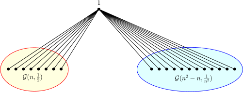
Figure 1. Illustration for Example 2.4.

Note that $|E(G_{n})|=\frac{7}{4}n^{2}(1+o_{P}(1))$. In this case, (1.7) holds with $\sigma_{11}=\frac{4}{7}$ and $\sigma_{st}=0$ for $(s,t)\neq(1,1)$. To check Assumption 1.3, we remove the vertices $\{1,2,\ldots,K\}$ from $G_{n}$ to obtain $G_{n,K}$. Note that after vertex $1$, with high probability, the next $K-1$ top vertices are the $K-1$ top vertices of $\mathcal{G}(n,\frac{1}{2})$. Let $H_{n,K}$ be the graph obtained by removing the top $K-1$ vertices from $\mathcal{G}(n,\frac{1}{2})$. Thus with high probability, $G_{n,K}$ is a disjoint union of two subgraphs which are isomorphic to $\mathcal{G}(n^{2}-n,\frac{1}{n^{2}})$ and $H_{n,K}$. By [28, Corollary 1.2], the maximum eigenvalue $\lambda_{\mathrm{max}}(\mathcal{G}(n^{2}-n,\frac{1}{n^{2}}))=o_{P}(n)$. Note that $\lambda_{\mathrm{max}}(\mathcal{G}(n,\frac{1}{2}))=(1+o_{P}(1))\frac{1}{2}n$ and the other eigenvalues of $\mathcal{G}(n,\frac{1}{2})$ are $o_{P}(n)$. Since $H_{n,K}$ is a subgraph of $\mathcal{G}(n,\frac{1}{2})$, by interlacing of eigenvalues $\lambda_{\mathrm{max}}({H}_{n,K})\leq(1+o_{P}(1))\frac{1}{2}n$ and other eigenvalues of $H_{n,K}$ are $o_{p}(n)$. Note that the largest eigenvalue of a graph is bounded below by the average degree of the graph. Thus,

$$\lambda_{\mathrm{max}}({H}_{n,K})\geq\frac{2}{n-K+1}|E(H_{n,K})|\geq\frac{2}{n-K+1}\left(|E(\mathcal{G}(n,\tfrac{1}{2})|-(K-1)(n-1)\right).$$

Since $E(\mathcal{G}(n,\frac{1}{2}))=(1+o_{p}(1))\frac{1}{4}n^{2}$, from the above inequality we have $\lambda_{\mathrm{max}}(H_{n,K})=(1+o_{P}(1))\frac{1}{2}n$ and the other eigenvalues of $H_{n,K}$ are $o_{P}(n)$. Hence, (1.8) holds with $\rho_{1}=\frac{1}{\sqrt{7}}$ and $\rho_{s}=0$ for $s\geq 2$. Thus, by Theorem 1.4,

$$S_{G_{n}}(\bm{X}_{n})\stackrel{{\scriptstyle D}}{{\rightarrow}}N(0,\tfrac{4}{7}X_{1}^{2})+\tfrac{1}{2\sqrt{7}}(\chi_{1}^{2}-1)+N(0,\tfrac{5}{14}),$$

where the three terms above are mutually independent.

Finally, we construct an example where the $\Sigma$ matrix appearing in Assumption 1.2 is infinite. For this we consider a disjoint union of star graphs with growing sizes.

Example 2.5.

Suppose $G_{n}=\bigsqcup_{s=0}^{n}K_{1,2^{s}}$, that is, $G_{n}$ is the disjoint union of $n$ stars where the $s$-th star has size $2^{s}$, for $1\leq s\leq n$. We label the vertices in non-increasing order of their degrees. Then, since $|E(G_{n})|=\sum_{s=1}^{n}2^{s}=2^{n+1}-2$, we have

$$\sigma_{ss}=2^{-s},\text{ for }s\geq 1\text{ and }\sigma_{st}=0\text{ for all }s\neq t.$$

Next, note that the graph $G_{n,K}$ obtained by removing the $K$ highest degree vertices from $G_{n}$ is still a disjoint unions of stars. In particular, $G_{n,K}=\bigsqcup_{s=1}^{n-K}K_{1,2^{s}}$. This implies, the largest eigenvalue $\lambda_{\mathrm{max}}(G_{n,K})=2^{(n-K)/2}$ and hence,

$$\frac{\lambda_{\mathrm{max}}(G_{n,K})}{\sqrt{|E(G_{n})|}}=\frac{2^{(n-K)/2}}{\sqrt{2^{n+1}-2}}=\frac{1}{\sqrt{2^{K+1}-2^{K+1-n}}}\rightarrow 0,$$

taking $n\to\infty$ followed by $K\to\infty$. This implies, (1.8) holds with $\rho_{s}=0$ for all $s\geq 1$. Thus, by Theorem 1.4, in this case

$$S_{G_{n}}(\bm{X}_{n})\stackrel{{\scriptstyle D}}{{\rightarrow}}N\left(0,\sum_{s=1}^{\infty}\frac{1}{2^{s}}X_{s}^{2}\right).$$

3. Proofs of Theorem 1.4 and Theorem 1.7

Throughout the proof we will assume that the vertices of the graph $G_{n}$ are labelled by $\llbracket n\rrbracket:=\{1,2,\ldots,n\}$ in non-increasing order of the degrees. The first step in the proof of Theorem 1.4 is a truncation argument which shows that we can replace the random variables $\bm{X}_{n}=(X_{1},\ldots,X_{n})^{\top}$ by their truncated versions (properly centered and scaled) without changing the asymptotic distribution of $S_{G_{n}}(\bm{X}_{n})$. Towards this recall from (1.10) that $a_{M}:=\mathbb{E}[X_{1}\bm{1}\{|X_{1}|\leq M\}]$, $b_{M}:=\operatorname{Var}[X_{1}\bm{1}\{|X_{1}|\leq M\}]$, and $\bm{X}_{n,M}=(X_{1,M},\ldots,X_{n,M})^{\top}$, where

$$X_{u,M}:=b_{M}^{-\frac{1}{2}}(X_{u}\bm{1}\{|X_{u}|\leq M\}-a_{M}),$$

for $1\leq u\leq n$. Then with $S_{G_{n}}$ as defined in (1.6), the following lemma shows that the asymptotic distributions of $S_{G_{n}}(\bm{X}_{n,M})$ and $S_{G_{n}}(\bm{X}_{n})$ are the same, as $n\rightarrow\infty$ followed by $M\rightarrow\infty$.

Lemma 3.1.

For every $\varepsilon>0$,

$$\lim_{M\to\infty}\sup_{n\geq 1}\mathbb{P}(|S_{G_{n}}(\bm{X}_{n})-S_{G_{n}}(\bm{X}_{n,M})|>\varepsilon)=0.$$

Proof.

Note that

$$b_{M}^{-1}S_{G_{n}}(\bm{X}_{n})-S_{G_{n}}(\bm{X}_{n,M}) =\frac{b_{M}^{-1}}{\sqrt{|E(G_{n})|}}\sum_{1\leq u<v\leq n}a_{u,v}(X_{u}X_{v}-b_{M}X_{u,M}X_{v,M}).$$ (3.1)

Now, since $X_{u}-b_{M}^{\frac{1}{2}}X_{u,M}=X_{u}\bm{1}\{|X_{u}|>M\}+a_{M}$,

$$X_{u}X_{v}-b_{M}X_{u,M}X_{v,M} =X_{u}X_{v}-b_{M}^{\frac{1}{2}}X_{u,M}X_{v}+b_{M}^{\frac{1}{2}}X_{u,M}X_{v}-b_{M}X_{u,M}X_{v,M}$$

$$=(X_{u}-b_{M}^{\frac{1}{2}}X_{u,M})X_{v}+b_{M}^{\frac{1}{2}}X_{u,M}(X_{v}-b_{M}^{\frac{1}{2}}X_{v,M})$$

$$=(X_{u}\bm{1}\{|X_{u}|>M\}+a_{M})X_{v}+b_{M}^{\frac{1}{2}}X_{u,M}(X_{v}\bm{1}\{|X_{v}|>M\}+a_{M}).$$

Thus, from (3.1),

$$b_{M}^{-1}S_{G_{n}}(\bm{X}_{n})-S_{G_{n}}(\bm{X}_{n,M})=T_{1}+T_{2},$$

where

$$T_{1}:=\frac{b_{M}^{-1}}{\sqrt{|E(G_{n})|}}\sum_{1\leq u<v\leq n}a_{u,v}(X_{u}\bm{1}\{|X_{u}|>M\}+a_{M})X_{v}$$

and

$$T_{2}:=\frac{b_{M}^{-\frac{1}{2}}}{\sqrt{|E(G_{n})|}}\sum_{1\leq u<v\leq n}a_{u,v}X_{u,M}(X_{v}\bm{1}\{|X_{v}|>M\}+a_{M})$$

Now, since the collection $\{X_{u}\}_{1\leq u\leq n}$ are uncorrelated with mean 0 and variance $1$ and $\mathbb{E}[X_{1}\bm{1}\{|X_{1}|>M\}]=-a_{M}$,

$$\operatorname{Var}\left[T_{1}\right]=\frac{1}{b_{M}^{2}}\operatorname{Var}[X_{1}\bm{1}\{|X_{1}|>M\}]\quad\text{ and }\quad\operatorname{Var}[T_{2}]=\frac{1}{b_{M}}\operatorname{Var}[X_{1}\bm{1}\{|X_{1}|>M\}].$$

Thus, by Markov’s inequality and using the fact that $\operatorname{Var}[A+B]\leq 2\operatorname{Var}[A]+2\operatorname{Var}[B]$ we have

$$\mathbb{P}(|S_{G_{n}}(\bm{X}_{n})-S_{G_{n}}(\bm{X}_{n,M})|>\varepsilon)$$

$$\leq\mathbb{P}\left(\left|1-\frac{1}{b_{M}}\right||S_{G_{n}}(\bm{X}_{n})|>\tfrac{\varepsilon}{2}\right)+\mathbb{P}\left(\left|b_{M}^{-1}S_{G_{n}}(\bm{X}_{n})-S_{G_{n}}(\bm{X}_{n,M})\right|>\tfrac{\varepsilon}{2}\right)$$

$$\lesssim\frac{1}{\varepsilon^{2}}\left(1-\frac{1}{b_{M}}\right)^{2}+\frac{1}{\varepsilon^{2}}\left(\frac{1}{b_{M}^{2}}+\frac{1}{b_{M}}\right)\operatorname{Var}[X_{1}\bm{1}\{|X_{1}|>M\}].$$

This gives the desired result, since $b_{M}\to 1$ and $\operatorname{Var}[X_{1}\bm{1}\{|X_{1}|>M\}]\to 0$ as $M\to\infty$. ∎

The above lemma shows that it suffices to derive the limiting distribution of $S_{G_{n}}(\bm{X}_{n,M})$. One of the advantages of working with $\bm{X}_{n,M}$ is that $S_{G_{n}}(\bm{X}_{n,M})$ has all finite moments. In fact, the moment generating function of $S_{G_{n}}(\bm{X}_{n,M})$ exists in an interval containing $0$ (see Lemma A.2). To this end, fix $M\geq 1$. The proof now of Theorem 1.4 now proceeds by partitioning the set of vertices $\llbracket n\rrbracket=\{1,2,\ldots,n\}$ into the following three parts: Towards this, fix $K_{1},K_{2}\geq 1$ and define

$$V_{1}:=\left\llbracket 1,\left\lfloor K_{1}\right\rfloor\right\rrbracket,~{}V_{2}:=\left\llbracket\left\lfloor K_{1}\right\rfloor+1,\left\lfloor K_{2}\sqrt{|E(G_{n})|}\right\rfloor\right\rrbracket,~{}\text{and}~{}V_{3}:=\left\llbracket\left\lfloor K_{2}\sqrt{|E(G_{n})|}\right\rfloor+1,n\right\rrbracket.$$ (3.2)

Hereafter, for $1\leq s\leq 3$, we set $n_{s}:=|V_{s}|$. Note that since the vertices of $G_{n}$ are arranged in non-increasing order of the degrees, we refer to the vertices in $V_{1},V_{2},V_{3}$ as the ‘high’ degree, ‘medium’ degree, and ‘low’ degree vertices, respectively. The adjacency matrix $A(G_{n})$ can then be decomposed as a $3\times 3$ block matrix as follows:

$$A(G_{n})=\begin{pmatrix}A_{11}&A_{12}&A_{13}\\ A_{21}&A_{22}&A_{23}\\ A_{31}&A_{32}&A_{33}\end{pmatrix},$$ (3.3)

where $A_{st}$ is a matrix of order $n_{s}\times n_{t}$ which encodes the edge connections between the vertex sets $V_{s}$ and $V_{t}$ in $G_{n}$, for $1\leq s,t\leq 3$. (Recall that in the Introduction we referred to $A_{11}$, $A_{12}$, $A_{13}$, $A_{22}$, $A_{23}$, and $A_{33}$, as the high-to-high (hh), high-to-medium (hm), high-to-low (hl), medium-to-medium (mm), medium-to-low (ml), and low-to-low (ll) edges, respectively.) The proof of Theorem 1.4 involves deriving the asymptotic contributions of these 6 terms. Before proceeding to the technical details, we provide an outline of the proof below (refer to Figure 2):

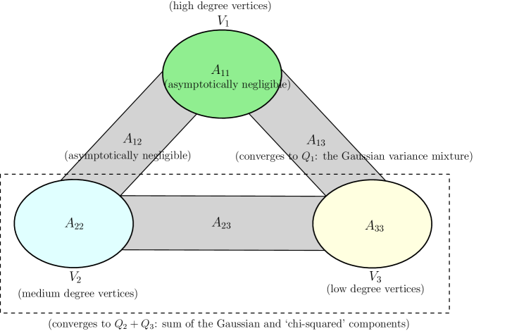
Figure 2. The partition of the vertices and the edges of the graph $G_{n}$ as in the proof of Theorem 1.4.

1. The first step in the proof of Theorem 1.4 is to show that the variables corresponding to medium and low degree vertices, that is, those in the sets $V_{2}$ and $V_{3}$ can be replaced by standard Gaussian random variables without incurring any asymptotic error (see Proposition 3.2 in Section 3.1). The proof uses Lindeberg’s method of replacing the non-Gaussian variables by Gaussian variables one by one and using Taylor expansion to get approximation bounds on the error.

2. The next step is to show that the contribution to $S_{G_{n}}$ from $A_{11}$ and $A_{12}$ are negligible asymptotically. This follows by a simple second moment argument and the definitions of the sets $V_{1},V_{2}$ (see Lemma 3.3 in Section 3.1).

3. Then in Section 3.2 we show that the contributions to $S_{G_{n}}$ from $A_{13}$ is asymptotically independent in moments from the rest (see Proposition 3.4). The proof of Proposition 3.4 proceeds in two steps:

   • First we show that the contribution from $A_{33}$ is asymptotically independent in moments from the joint contributions of $A_{13}$, $A_{22}$, and $A_{23}$ (Lemma 3.5). This involves expressing moments as a sum over subgraphs of $G_{n}$ and then estimating the subgraph counts using the results from extremal combinatorics [1, 21] and the relevant degree bounds on the sets $V_{2},V_{3}$.

   • The second step is to show that the contribution from $A_{13}$ is asymptotically independent from contributions of $A_{22}$ and $A_{23}$ (Lemma 3.6). For this we show that the covariance between $A_{13}$ and $A_{22}\bigcup A_{23}$ vanishes in the limit and then leverage properties of the Gaussian distribution (recall that the variables in $V_{2}$ and $V_{3}$ can be replaced by standard Gaussian variables by step (1) above) to establish the asymptotic independence. This combined with the previous step establishes the independence of $A_{13}$ from the rest.

4. Next, in Section 3.3 we compute the limiting distribution corresponding to $A_{13}$ for a fixed truncation level $M$. Here, the limit is a normal variance mixture, where the random variance is a quadratic form determined by the matrix $\Sigma$ (as defined in Assumption 1.2), and the truncated variables $\{X_{u,M}\}_{u\geq 1}$.

5. In Section 3.4 we compute the limiting distribution corresponding to $A_{22}\bigcup A_{23}$. Since the variables in $V_{2}\bigcup V_{3}$ have been replaced by standard Gaussians, we can use the spectral decomposition of $A_{n,K}$ (the adjacency matrix of the truncated graph $G_{n,K}$) and Assumption 1.2 to show that this component converges to $Q_{2}+Q_{3}$ as defined in (1.9).

6. Finally, in Section 3.5 we derive the limit of the $Q_{1,M}$ (the distribution obtained in step (4) above) as $M\to\infty$ limit, thus completing the proof of Theorem 1.4. Using the result in Theorem 1.4 along a subsequence we also prove Theorem 1.7 in Section 3.5.

3.1. Gaussian Replacements

Recall the partition of the vertex set $\llbracket n\rrbracket=\{1,2,\ldots,n\}$ into the sets $V_{1},V_{2},V_{3}$ from (3.2). Then we can partition the random vector $\bm{X}_{n,M}=(X_{1,M},X_{2,M},\ldots,X_{n,M})^{\top}$ as

$$\bm{X}_{n,M}=((\bm{X}_{n,M}^{(1)})^{\top},(\bm{X}_{n,M}^{(2)})^{\top},(\bm{X}_{n,M}^{(3)})^{\top})^{\top},$$

where $\bm{X}_{n,M}^{(s)}=((X_{j,M}))_{j\in V_{s}}$ is a $n_{s}$-dimensional vector, for $s\in\{1,2,3\}$. We now show that one can replace the variables in $\bm{X}_{n,M}^{(2)}$ and $\bm{X}_{n,M}^{(3)}$ with standard Gaussian random variables without changing the limiting distribution of $S_{G_{n}}(\bm{X}_{n,M})$. Towards this end, consider

$$\bm{Z}_{n}^{\top}:=(Z_{1},\ldots,Z_{n}):=((\bm{Z}_{n}^{(1)})^{\top},(\bm{Z}_{n}^{(2)})^{\top},(\bm{Z}_{n}^{(3)})^{\top}),$$ (3.4)

where $Z_{1},Z_{2},\ldots$ are i.i.d. $N(0,1)$ (which are also independent of the collection $\{X_{i}\}_{1\leq i\leq n}$) and $\bm{Z}_{n}^{(s)}=((Z_{j}))_{j\in V_{s}}$ is a $n_{s}$-dimensional vector, for $1\leq s\leq 3$.

Proposition 3.2.

Let $S_{G_{n}}$ be as defined in (1.6) and $h:\mathbb{R}\to\mathbb{C}$ be a bounded, three times continuously differentiable function with $\|h^{\prime\prime\prime}\|\leq L<\infty$.

1. Then

   $$|\mathbb{E}[h(S_{G_{n}}({\bm{X}}_{n}))]-\mathbb{E}[h(S_{G_{n}}({\bm{Z}}_{n}))]|\lesssim_{L}\frac{\max_{1\leq u\leq n}d_{u}}{|E(G_{n})|}.$$

2. Moreover,

   $$\lim_{K_{1},K_{2}\to\infty}\sup_{n\geq K_{1}}\left|\mathbb{E}\left[h\left(S_{G_{n}}\left(\bm{X}_{n,M}\right)\right)\right]-\mathbb{E}\left[h\left(S_{G_{n}}\left(((\bm{X}_{n,M}^{(1)})^{\top},(\bm{Z}_{n}^{(2,3)})^{\top})^{\top}\right)\right)\right]\right|=0,$$ (3.5)

   where $\bm{Z}_{n}^{(2,3)}:=((\bm{Z}_{n}^{(2)})^{\top},(\bm{Z}_{n}^{(3)})^{\top})^{\top}$.

Proof of Proposition 3.2.

For each $0\leq u\leq n$, define

$$\bm{W}_{u} :=(X_{1},X_{2},\ldots,X_{n-u},Z_{n-u+1},\ldots,Z_{n})^{\top},$$ (3.6)

In other words, the vector $\bm{W}_{u}$ is obtained by replacing the last $u$ elements of the vector $\bm{X}$ with the last $u$ elements of the vector $\bm{Z}$. Note that $\bm{W}_{0}=\bm{X}$ and $\bm{W}_{n}=\bm{Z}$, and the vectors $\{\bm{W}_{u}\}_{0\leq u\leq n}$ serves an interpolation between $\bm{X}_{n}$ and $\bm{Z}_{n}$, obtaining replacing one coordinate at a time.

Now, set

$$T_{u}:=S_{G_{n}}(\bm{W}_{u}),$$ (3.7)

and fix a bounded thrice continuously differentiable function $h:\mathbb{R}\to\mathbb{C}$ with $\|h^{\prime\prime\prime}\|\leq L$. We claim that for each $0\leq u\leq n$ we have

$$\left|\mathbb{E}[h(T_{u+1})]-\mathbb{E}[h(T_{u})]\right|\lesssim_{L}\left(\frac{d_{n-u}}{|E(G_{n})|}\right)^{\frac{3}{2}}.$$ (3.8)

Assuming (3.8) we first show how to complete the proof of Proposition 3.2. To this end, summing (3.8) over $u$ from $0$ to $n-1$ gives

$$|\mathbb{E}h(S_{G_{n}}({\bm{X}}_{n}))-\mathbb{E}h(S_{G_{n}}({\bm{Z}}_{n}))|=|\mathbb{E}h(T_{(0)})-h(T_{(n)})| \lesssim_{L}\sum_{u=1}^{n}\Big{(}\frac{d_{u}}{|E(G_{n})|}\Big{)}^{3/2}$$

$$\leq 2\sqrt{\frac{\max_{1\leq u\leq n}d_{u}}{|E(G_{n})|}},$$

which verifies part (a).

For part (b), we will invoke (3.7) with $X_{n}$ replaced by $X_{n,M}$. With this choice, observe that

$$T_{(n-\lceil K_{1}\rceil)}=S_{G_{n}}\left(\left((\bm{X}_{n,M}^{(1)})^{\top},(\bm{Z}_{n}^{(2,3)})^{\top}\right)^{\top}\right)\quad\text{ and }\quad T_{(0)}=S_{G_{n}}\left(\bm{X}_{n,M}\right).$$

Therefore, summing over $u$ from 0 to $n-\lceil K_{1}\rceil-1$ on both sides of (3.8) gives,

$$\left|\mathbb{E}\left[h\left(S_{G_{n}}\left(\bm{X}_{n,M}\right)\right)\right]-\mathbb{E}\left[h\left(S_{G_{n}}\left(((\bm{X}_{n,M}^{(1)})^{\top},(\bm{Z}_{n}^{(2,3)})^{\top})^{\top}\right)\right)\right]\right| =\left|\mathbb{E}[h(T_{(n-\lceil K_{1}\rceil)})]-\mathbb{E}[h(T_{(0)})]\right|$$

$$\lesssim_{L}\sum_{u=\lceil K_{1}\rceil+1}^{n}\left(\frac{d_{u}}{|E(G_{n})|}\right)^{\frac{3}{2}}.$$ (3.9)

As the vertices $\llbracket n\rrbracket$ are labeled such that the degrees of $G_{n}$ are arranged in non-increasing order, for all $u\geq\lceil K_{1}\rceil+1$,

$$d_{u}\leq\frac{1}{u}\sum_{v=1}^{u}d_{v}\leq\frac{1}{u}\sum_{v=1}^{n}d_{v}=\frac{2|E(G_{n})|}{u}\leq\frac{2|E(G_{n})|}{\lceil K_{1}\rceil+1}.$$ (3.10)

Thus,

$$\sum_{u=\lceil K_{1}\rceil+1}^{n}\left(\frac{d_{u}}{|E(G_{n})|}\right)^{\frac{3}{2}}\lesssim\frac{1}{\sqrt{\lceil K_{1}\rceil+1}}\sum_{u=\lceil K_{1}\rceil+1}^{n}\frac{d_{u}}{|E(G_{n})|}\lesssim\frac{1}{\sqrt{\lceil K_{1}\rceil+1}}.$$

Using the above estimate in the RHS of (3.1) and taking the appropriate limits the result in (3.5) follows.

∎

Proof of (3.8).

For $0\leq u\leq n$ recall the definition of $\bm{W}_{u}$ from (3.6). In this proof, we will denote the $v$-th coordinate of $\bm{W}_{u}$ as $W_{u,v}$, for $1\leq v\leq n$. For $0\leq u\leq n$, define the following notations:

$$Q_{u} :=\frac{1}{\sqrt{|E(G_{n})|}}\sum_{\begin{subarray}{c}1\leq v\leq n\\ v\neq n-u\end{subarray}}a_{n-u,v}W_{u,v},\quad R_{u}:=\frac{1}{\sqrt{|E(G_{n})|}}\sum_{\begin{subarray}{c}1\leq v<v^{\prime}\leq n\\ v,v^{\prime}\neq n-u\end{subarray}}a_{v,v^{\prime}}W_{u,v}W_{u,v^{\prime}},$$

Now, recall the definition of $T_{u}$ from (3.7) and observe the following:

1. $T_{u}=X_{n-u}Q_{u}+R_{u}$ and $T_{u+1}=Z_{n-u}Q_{u}+R_{u}$,

2. $X_{n-u}$ and $Z_{n-u}$ are independent of $(Q_{u},R_{u})$.

The second observation implies

$$\mathbb{E}\left[{Z_{n-u}Q_{u}}h^{\prime}\left({R_{u}}\right)\right]=\mathbb{E}\left[{X_{n-u}Q_{u}}h^{\prime}\left({R_{u}}\right)\right]$$

and

$$\mathbb{E}\left[{Z_{n-u}^{2}Q_{u}^{2}}h^{\prime\prime}\left({R_{u}}\right)\right]=\mathbb{E}\left[{X_{n-u}^{2}Q_{u}^{2}}h^{\prime\prime}\left({R_{u}}\right)\right].$$

Using the above identifies and the triangle inequality gives

$$\left|\mathbb{E}[h(T_{u+1})-h(T_{u})]\right|$$

$$\leq\left|\mathbb{E}\left[h(T_{u+1})-h(R_{u})-Z_{n-u}Q_{u}h^{\prime}(R_{u})-\tfrac{1}{2}Z_{n-u}^{2}(Q_{u})^{2}h^{\prime\prime}(R_{u})\right]\right|$$

$$\hskip 71.13188pt+\left|\mathbb{E}\left[h(T_{u})-h(R_{u})-X_{n-u}Q_{u}h^{\prime}(R_{u})-\tfrac{1}{2}X_{n-u}^{2}(Q_{u})^{2}h^{\prime\prime}(R_{u})\right]\right|$$

$$\leq\tfrac{L}{6}\left\{\mathbb{E}\left|Z_{n-u}^{3}Q_{u}^{3}\right|+\mathbb{E}\left|X_{n-u}^{3}Q_{u}^{3}\right|\right\}$$

$$\lesssim_{L}\mathbb{E}\left|Q_{u}^{3}\right|(\mathbb{E}|X_{n-u}^{3}|+\mathbb{E}|Z_{n-u}^{3}|).$$ (3.11)

Note that $\{W_{u,v}\}_{1\leq v\leq n}$ are independent mean $0$ variance $1$ random variables with finite fourth moments. Thus, by Hölder’s inequality,

$${|E(G_{n})|}^{\frac{3}{2}}\mathbb{E}\left|Q_{u}^{3}\right| \leq{|E(G_{n})|}^{\frac{3}{2}}\left(\mathbb{E}\left[Q_{u}^{4}\right]\right)^{\frac{3}{4}}$$

$$\lesssim\left[\sum_{\begin{subarray}{c}1\leq v\leq n\\ v\neq n-u\end{subarray}}a_{n-u,v}\mathbb{E}[W_{u,v}^{4}]+\sum_{\begin{subarray}{c}1\leq v\neq v^{\prime}\leq n\\ v,v^{\prime}\neq n-u\end{subarray}}a_{n-u,v}a_{n-u,v^{\prime}}\mathbb{E}[W_{u,v}^{2}]\mathbb{E}[W_{u,v^{\prime}}^{2}]\right]^{\frac{3}{4}}$$

$$\lesssim\left[\sum_{\begin{subarray}{c}1\leq v\leq n\\ v\neq n-u\end{subarray}}a_{n-u,v}+\left(\sum_{\begin{subarray}{c}1\leq v\leq n\\ v\neq n-u\end{subarray}}a_{n-u,v}\right)^{2}\right]^{\frac{3}{4}}$$

$$\lesssim d_{n-u}^{\frac{3}{2}}.$$ (3.12)

As $X_{n-u}$ and $Z_{n-u}$ have finite third moments, combining (3.11) and (3.1) the result in (3.8) follows. ∎

Now, recalling the block decomposition of the matrix $A(G_{n})$ from (3.3) gives,

$$S_{G_{n}} \left(((\bm{X}_{n,M}^{(1)})^{\top},(\bm{Z}_{n}^{(2,3)})^{\top})^{\top}\right)$$

$$:=U_{11,n,M}+U_{12,n,M}+U_{13,n,M}+U_{22,n}+U_{23,n}+U_{33,n},$$ (3.13)

where

$$U_{11,n,M} :=\frac{(\bm{X}_{n,M}^{(1)})^{\top}A_{11}\bm{X}_{n,M}^{(1)}}{2\sqrt{|E(G_{n})|}}, U_{12,n,M} :=\frac{(\bm{X}_{n,M}^{(1)})^{\top}A_{12}\bm{Z}_{n}^{(2)}}{\sqrt{|E(G_{n})|}}, U_{13,n,M} :=\frac{\bm{X}_{n,M}^{(1)}A_{13}(\bm{Z}_{n}^{(3)})^{\top}}{2\sqrt{|E(G_{n})|}},$$

$$U_{22,n} :=\frac{(\bm{Z}_{n}^{(2)})^{\top}A_{22}\bm{Z}_{n}^{(2)}}{2\sqrt{|E(G_{n})|}}, U_{23,n} :=\frac{(\bm{Z}_{n}^{(2)})^{\top}A_{23}\bm{Z}_{n}^{(3)}}{\sqrt{|E(G_{n})|}}, U_{33,n} :=\frac{(\bm{Z}_{n}^{(3)})^{\top}A_{33}\bm{Z}_{n}^{(3)}}{2\sqrt{|E(G_{n})|}}.$$

(Note that $U_{13,n,M},U_{22,n},U_{23,n},$ and $U_{33,n}$ depends on $K_{1}$ and $K_{2}$ as well (recall (3.2)), but we suppress this dependence for notational convenience.)

The proof of Theorem 1.4 now proceeds by analyzing the six terms in (3.1). The first step is to show that the terms $U_{11,n,M}$ and $U_{12,n,M}$ are negligible asymptotically.

Lemma 3.3.

For $U_{11,n,M}$ and $U_{12,n,M}$ as defined above the following hold:

$$\lim_{n\to\infty}\mathbb{P}(|U_{11,n,M}+U_{12,n,M}|>\varepsilon)=0.$$

Proof.

Using the fact that $\operatorname{Var}[A+B]\leq 2\operatorname{Var}[A]+2\operatorname{Var}[B]$ and an application of Markov inequality shows that

$$\mathbb{P}\left(|U_{11,n,M}+U_{12,n,M}|>\varepsilon\right) \lesssim\frac{1}{\varepsilon^{2}|E(G_{n})|}\left\{\operatorname{Var}[(\bm{X}_{n,M}^{(1)})^{\top}A_{11}\bm{X}_{n,M}^{(1)}]+\operatorname{Var}[(\bm{X}_{n,M}^{(1)})^{\top}A_{12}\bm{Z}_{n}^{(2)}]\right\}$$

$$\lesssim\frac{1}{\varepsilon^{2}|E(G_{n})|}\left\{\mathrm{tr}(A_{11}^{2})+\mathrm{tr}(A_{12}^{2})\right\}$$

$$\leq\frac{1}{\varepsilon^{2}|E(G_{n})|}\left\{|V_{1}|^{2}+|V_{1}||V_{2}|\right\}$$

$$\leq\frac{1}{\varepsilon^{2}|E(G_{n})|}\left[K_{1}^{2}+K_{1}K_{2}\sqrt{|E(G_{n})|}\right].$$

The expression above goes to zero as $n\to\infty$ followed, for all $K_{1},K_{2}$ fixed. This completes the proof of the lemma. ∎

3.2. Asymptotic Independence of $U_{13,n,M}$ and $U_{22,n}+U_{23,n}+U_{33,n}$

The goal of this section is to show that $U_{13,n,M}$ is asymptotically independent of $U_{22,n}+U_{23,n}+U_{33,n}$ in moments. This is formalized in the following proposition:

Proposition 3.4.

Fix $M$ large enough such that $U_{13,n,M}$ is well defined in (3.1). Then for all non-negative integers $a,b$,

$$\lim_{K_{1}\to\infty}\limsup_{n\to\infty}\left|\mathbb{E}\left[U_{13,n,M}^{a}(U_{22,n}+U_{23,n}+U_{33,n})^{b}\right]-\mathbb{E}\left[U_{13,n,M}^{a}\right]\mathbb{E}\left[(U_{22,n}+U_{23,n}+U_{33,n})^{b}\right]\right|=0.$$

Proof of Proposition 3.4.

The first step in the proof is to show that $U_{33,n}$ is asymptotically independent of the triplet $(U_{13,n,M},U_{22,n},U_{23,n})$ in moments. This is shown in the following lemma which is proved in Section 3.2.1.

Lemma 3.5.

For all non-negative integers $a,b,c,d$ the following holds:

$$\lim_{K_{1},K_{2}\to\infty}\limsup_{n\to\infty}\left|\mathbb{E}\left[U_{13,n,M}^{a}U_{22,n}^{b}U_{23,n}^{c}U_{33,n}^{d}\right]-\mathbb{E}\left[U_{13,n,M}^{a}U_{22,n}^{b}U_{23,n}^{c}\right]\mathbb{E}\left[U_{33,n}^{d}\right]\right|=0.$$

Next, we show that $U_{13,n,M}$ is asymptotically independent of $U_{22,n}+U_{23,n}$ using the Gaussian structure. This is described in the following lemma which is proved in Section 3.2.2.

Lemma 3.6.

For any $t_{1},t_{2}\in\mathbb{R}$,

$$\lim_{K_{1}\to\infty}\limsup_{n\to\infty}\left|\mathbb{E}[e^{\bm{i}t_{1}U_{13,n,M}+it_{2}(,U_{22,n}+U_{23,n})}]-\mathbb{E}[e^{\bm{i}t_{1}U_{13,n,M}}]\mathbb{E}[e^{\bm{i}t_{2}(U_{22,n}+U_{23,n})}]\right|=0.$$

Given the above two lemmas, the proof of Proposition 3.4 can be completed easily. Recall that

$$U_{13,n,M}:=\frac{1}{2\sqrt{|E(G_{n})|}}\bm{X}_{n,M}^{(1)}A_{13}(\bm{Z}_{n}^{(3)})^{\top}.$$

For each fixed $M$, the truncated random variables $\{X_{u,M}\}_{1\leq u\leq n}$ and $\{Z_{u}\}_{1\leq u\leq n}$ are centered, bounded, and hence, sub-Gaussian. Therefore, the matrix $\frac{1}{2\sqrt{|E(G_{n})|}}A_{13}$ satisfies the condition (A.2) in Appendix A. Similarly, since $U_{22,n},U_{23,n},$ and $U_{33,n}$ involve Gaussian random variables, the corresponding matrices satisfies (A.2). Thus, by Lemma A.2 there exists $\delta>0$ such that

$$\sup_{|t|\leq\delta}\sup_{K_{1},K_{2}\geq 1}\sup_{n\geq 1}\left\{\mathbb{E}[e^{tU_{13,n,M}}]+\mathbb{E}[e^{tU_{22,n}}]+\mathbb{E}[e^{tU_{23,n}}]+\mathbb{E}[e^{tU_{33,n}}]\right\}<\infty.$$ (3.14)

Now, let us denote

$$\mathcal{R}_{n,K_{1}}:=U_{13,n,M}\quad\text{and}\quad\mathcal{S}_{n,K_{1}}:=U_{22,n}+U_{23,n}.$$

By (3.14), we have $\{(\mathcal{R}_{n,K_{1}},\mathcal{S}_{n,K_{1}})\}_{n,K_{1}\geq 1}$ is a tight sequence of random variables. Therefore, passing through a double subsequence (in both $n,K_{1}$) we may assume $(\mathcal{R}_{n,K_{1}},\mathcal{S}_{n,K_{1}})$ converges in distribution, that is, there exists random variables $\mathcal{R},\mathcal{S}$ on $\mathbb{R}$ such that

$$(\mathcal{R}_{n,K_{1}},\mathcal{S}_{n,K_{1}})\stackrel{{\scriptstyle D}}{{\to}}(\mathcal{R},\mathcal{S}).$$

Now, Lemma 3.6 implies $\mathcal{R}$ and $\mathcal{S}$ must be independent. Therefore, by uniform integrability, for $a,b\geq 1$ integers,

$$\lim_{K_{1}\to\infty}\lim_{n\to\infty}\mathbb{E}[\mathcal{R}_{n,K_{1}}^{a}\mathcal{S}_{n,K_{1}}^{b}]=\mathbb{E}[\mathcal{R}^{a}\mathcal{S}^{b}]=\mathbb{E}[\mathcal{R}^{a}]\mathbb{E}[\mathcal{S}^{b}]=\lim_{K_{1}\to\infty}\lim_{n\to\infty}\mathbb{E}[\mathcal{R}_{n,K_{1}}^{a}]\mathbb{E}[\mathcal{S}_{n,K_{1}}^{b}],$$

and hence,

$$\lim_{K_{1}\to\infty}\lim_{n\to\infty}\left|\mathbb{E}[\mathcal{R}_{n,K_{1}}^{a}\mathcal{S}_{n,K_{1}}^{b}]-\mathbb{E}[\mathcal{R}_{n,K_{1}}^{a}]\mathbb{E}[\mathcal{S}_{n,K_{1}}^{b}]\right|=0.$$ (3.15)

Combining (3.15) with Lemma 3.5 and binomial theorem, the result in Proposition 3.4 follows. ∎

3.2.1. Proof of Lemma 3.5

In the method of moment calculations of Lemma 3.5, we will need to invoke various results from extremal graph theory. Towards this, we begin by recalling some basic definitions.

Extremal Graph Theory Background: For any graph $H$, denote the neighborhood of a set $S\subseteq V(H)$ by $N_{H}(S)=\{v\in V(H):\exists u\in S\text{ and }(u,v)\in E(H)\}$. Next, given two simple graphs $G=(V(G),E(G))$ and $H=(V(H),E(H))$, denote by $N(H,G)$ the number of isomorphic copies of $H$ in $G$, that is,

$$N(H,G)=\sum_{S\subset E(G):|S|=|E(H)|}\boldsymbol{1}\{G[S]\cong H\},$$

where the sum is over subsets $S$ of $E(G)$ with $|S|=|E(H)|$, and $G[S]$ is the subgraph of $G$ induced by the edges of $S$.

One of the fundamental problems in extremal graph theory is to estimate, for any fixed graph $H$, the quantity $N(H,G)$ over the class of graphs $G$ with a specified number of edges. More formally, for a positive integer $\ell\geq|E(H)|$, define

$$N(H,\ell):=\sup_{G:|E(G)|=\ell}N(H,G).$$

For the complete graph $K_{h}$, Erdős [19] determined the asymptotic behavior of $N(K_{h},\ell)$ as $\ell$ tends to infinity, which is also a special case of the celebrated Kruskal-Katona theorem. For a general graph $H$ this problem was settled by Alon [1] and later extended to hypergraphs by Friedgut and Kahn [21]. To explain this result we need the following definition:

Definition 3.7.

[42] For any graph $H=(V(H),E(H))$ define its fractional stable number $\gamma(H)$ as:

$$\gamma(H)=\max_{\begin{subarray}{c}\phi\in[0,1]^{V(H)},\\ \phi(x)+\phi(y)\leq 1\text{ for }(x,y)\in E(H)\end{subarray}}\sum_{v\in V(H)}\phi(v),$$ (3.16)

where $[0,1]^{V(H)}$ is the collection of all functions $\phi:V(H)\rightarrow[0,1]$. Moreover, the polytope $\mathscr{P}(H)$ defined by the set of constraint

$$\{\phi\in[0,1]^{V(H)}:\phi(u)+\phi(v)\leq 1~{}\textrm{for all}~{}\{u,v\}\in E(H)\}$$

is called the fractional stable set polytope of the graph $H$.

We now state Alon’s result [1] result (in the language of [21]) in the following theorem for ease of referencing:

Theorem 3.8 ([1, 21]).

For a fixed graph $H$, there exist two positive constants $C_{1}=C_{1}(H)$ and $C_{2}=C_{2}(H)$ such that for all $\ell\geq|E(H)|$,

$$C_{1}\ell^{\gamma(H)}\leq N(H,\ell)\leq C_{2}\ell^{\gamma(H)},$$

where $\gamma(H)$ is fractional stable number of $H$ as in Definition 3.7.

In the proof of Lemma 3.5 we will often need to deal with multi-graphs (instead of simple graphs). A multi-graph $H$ is a graph with no self-loops, where there might be more than one edge between two vertices. In this case, the set of edges $E(H)$ is a multi-set where the edges are counted with their multiplicities. For a simple graph $G$ and a multi-graph $H$ define

$$M(H,G)=\sum_{e_{1}\in E(G)}\sum_{e_{2}\in E(G)}\cdots\sum_{e_{|E(H)|}\in E(G)}\boldsymbol{1}\{G[e_{1},e_{2},\ldots e_{|E(H)|}]\cong H\},$$

where $G[e_{1},e_{2},\ldots e_{|E(H)|}]$ is the multi-subgraph of $G$ formed by the edges $e_{1},e_{2},\ldots,e_{|E(H)|}$. In other words, $M(G,H)$ is the number of multi-subgraphs of $G$ isomorphic to the multi-graph $H$. It is easy to see that $M(H,G)\lesssim_{H}N(H_{S},G)$, where $H_{S}$ is the simple graph obtained from $H$ by replacing the edges between the vertices which occur more than once by a single edge. Moreover, the definition of the fractional stable number in (3.16) extends verbatim to any multi-graph $H$. In fact, since the constraint for each multiple edges between a pair of vertices is identical, it is clear that $\gamma(H)=\gamma(H_{S})$. Therefore, Theorem 3.8 implies,

$$M(H,G)\lesssim_{H}N(H_{S},G)\lesssim_{H}|E(G)|^{\gamma(H_{S})}.$$

Representing the Joint Moments in Terms of Multigraph Counts: With the above results we now proceed with the proof of Lemma 3.5. To begin with note that the result in Lemma 3.5 is trivial if either $a+b+c=0$ or $d=0$. Hence, we assume that both $a+b+c$ and $d$ are positive. Throughout this proof we will drop the subscript $n$ from $U_{22,n},U_{23,n},U_{33,n}$ and the subscripts $n$ and $M$ from $U_{13,n,M}$.

Now, let $E_{s,t}$ denote the set of all edges in $G_{n}$ with one vertex in $V_{s}$ and other in $V_{t}$, for $1\leq s,t\leq 3$ (recall the definitions of $V_{1},V_{2},V_{3}$ from (3.2)). Note that

$$\mathbb{E}\left[U_{13}^{a}U_{22}^{b}U_{23}^{c}U_{33}^{d}\right]-\mathbb{E}\left[U_{13}^{a}U_{22}^{b}U_{23}^{c}\right]\mathbb{E}\left[U_{33}^{d}\right] =\frac{1}{{|E(G_{n})|}^{\frac{a+b+c+d}{2}}}\sum_{\bm{u}}B_{\bm{u}}.$$ (3.17)

where the sum is over all tuples of the form:

$$\bm{u} :=\left(\{u_{1},v_{1}\},\ldots,\{u_{a},v_{a}\},\{u_{1}^{\prime},v_{1}^{\prime}\},\ldots,\{u_{b}^{\prime},v_{b}^{\prime}\},\right.$$

$$\hskip 142.26378pt\left.\{u_{1}^{\prime\prime},v_{1}^{\prime\prime}\},\ldots,\{u_{c}^{\prime\prime},v_{c}^{\prime\prime}\},\{u_{1}^{\prime\prime\prime},v_{1}^{\prime\prime\prime}\},\ldots,\{u_{d}^{\prime\prime\prime},v_{d}^{\prime\prime\prime}\}\right),$$ (3.18)

with $\{u_{1},v_{1}\},\ldots,\{u_{a},v_{a}\}\in E_{1,3}$, $\{u_{1}^{\prime},v_{1}^{\prime}\},\ldots,\{u_{b}^{\prime},v_{b}^{\prime}\}\in E_{2,2}$, $\{u_{1}^{\prime\prime},v_{1}^{\prime\prime}\},\ldots,\{u_{c}^{\prime\prime},v_{c}^{\prime\prime}\}\in E_{2,3}$, and $\{u_{1}^{\prime\prime\prime},v_{1}^{\prime\prime\prime}\},\ldots,\{u_{d}^{\prime\prime\prime},v_{d}^{\prime\prime\prime}\}\in E_{3,3}$; and

$$B_{\bm{u}} :=\mathbb{E}\left[\prod_{j=1}^{a}X_{u_{j},M}Z_{v_{j}}\prod_{j=1}^{b}Z_{u_{j}^{\prime}}Z_{v_{j}^{\prime}}\prod_{j=1}^{c}Z_{u_{j}^{\prime\prime}}Z_{v_{j}^{\prime\prime}}\prod_{j=1}^{d}Z_{u_{j}^{\prime\prime\prime}}Z_{v_{j}^{\prime\prime\prime}}\right]$$

$$\hskip 113.81102pt-\mathbb{E}\left[\prod_{j=1}^{a}X_{u_{j},M}Z_{v_{j}}\prod_{j=1}^{b}Z_{u_{j}^{\prime}}Z_{v_{j}^{\prime}}\prod_{j=1}^{c}Z_{u_{j}^{\prime\prime}}Z_{v_{j}^{\prime\prime}}\right]\mathbb{E}\left[\prod_{j=1}^{d}Z_{u_{j}^{\prime\prime\prime}}Z_{v_{j}^{\prime\prime\prime}}\right].$$

Since the terms with $B_{\bm{u}}=0$ does not contribute to (3.17), define $\mathcal{U}_{a,b,c,d}$ as the collection of all tuples $\bm{u}$ as in (3.2.1) for which $B_{\bm{u}}\neq 0$. Note, since all moments of $X_{1,M}$ are bounded, $|B_{\bm{u}}|\lesssim_{a,b,c,d,M}1$. Therefore, (3.17) can be bounded as:

$$\left|\mathbb{E}\left[U_{13}^{a}U_{22}^{b}U_{23}^{c}U_{33}^{d}\right]-\mathbb{E}\left[U_{13}^{a}U_{22}^{b}U_{23}^{c}\right]\mathbb{E}\left[U_{33}^{d}\right]\right| \lesssim_{a,b,c,d,M}\frac{1}{|E(G_{n})|^{\frac{a+b+c+d}{2}}}|\mathcal{U}_{a,b,c,d}|.$$ (3.19)

For every $\bm{u}\in\mathcal{U}_{a,b,c,d}$, let $H({\bm{u}})$ denote the multigraph formed by the edges in $\bm{u}$. Note that the multigraph $H({\bm{u}})$ has $a+b+c+d$ multi-edges, for each $\bm{u}\in\mathcal{U}_{a,b,c,d}$. As in simple graphs, we define the degree $d_{v}(H)$ of a vertex $v$ in a multigraph $H=(V(H),E(H))$ as the number of multi-edges of $H$ incident on the vertex $v$. Also, let $d_{\min}(H):=\min\{d_{v}(H):v\in V(H)\}$ denote the minimum degree of $H$.

Lemma 3.9.

For $H=H(\bm{u})$ with $\bm{u}\in\mathcal{U}_{a,b,c,d}$ the following hold:

1. $\gamma(H)\geq|V(H)|/2$.

2. $d_{\min}(H)\geq 2$ which implies $|V(H)|\leq a+b+c+d$. Moreover, if there exists a vertex $v^{\prime}\in V(H)$ such that $d_{v^{\prime}}(H)\geq 3$, then $|V(H)|<a+b+c+d$.

3. $\gamma(H)\leq|E(H)|/2=(a+b+c+d)/2$. Moreover, if there exists a vertex $v^{\prime}\in V(H)$ such that $d_{v^{\prime}}(H)\geq 3$ and $\varphi(v^{\prime})>0$, where $\varphi$ is an optimal solution to (3.16), then $|\gamma(H)|<(a+b+c+d)/2$.

4. $H_{S}$ contains a $2$-star as a subgraph with one edge in $E_{3,3}$.

Proof.

The proof of (1) follows by taking $\phi\equiv\frac{1}{2}$ in (3.16).

For (2), since $X_{1,M}$ and $Z\sim N(0,1)$ are both mean zero random variables, $B_{\bm{u}}$ is non zero only when each vertex index in $\bm{u}$ appears at least twice. This implies, $d_{\min}(H)\geq 2$. Hence,

$$2|V(H)|\leq|V(H)|d_{\min}(H)\leq\sum_{v\in V(H)}d_{v}(H)=2|E(H)|=2(a+b+c+d),$$

that is, $|V(H)|\leq a+b+c+d$. Now, suppose there exists $v^{\prime}\in V(H)$ such that $d_{v}(H)\geq 3$, then

$$2(|V(H)|-1)+3\leq\sum_{v\in V(H)}d_{v}(H)=2|E(H)|=2(a+b+c+d),$$

that is, $|V(H)|<a+b+c+d$.

Next, note that if $d_{\min}(H)\geq 2$, then for any function $\phi\in[0,1]^{V(H)}$ with $\phi(x)+\phi(y)\leq 1$, for $(x,y)\in E(H)$,

$$\sum_{x\in V(H)}\phi(x)\leq\frac{1}{d_{\min}(H)}\sum_{(x,y)\in E(H)}\{\phi(x)+\phi(y)\}\leq\frac{1}{2}|E(H)|.$$

which gives $\gamma(H)\leq\frac{1}{2}|E(H)|$. Now, suppose there exists $v^{\prime}\in V(H)$ such that $d_{v^{\prime}}(H)\geq 3$ and $\varphi(v^{\prime})\neq 0$. Then

$$|E(H)|\geq\sum_{(x,y)\in E(H)}\{\varphi(x)+\varphi(y)\}=\sum_{x\in V(H)}d_{x}(H)\varphi(x) \geq 3\varphi(v^{\prime})+2\sum_{x\in V(H)\backslash\{v^{\prime}\}}\varphi(x)$$

$$=2\gamma(H)+\varphi(v^{\prime}),$$

and the result in (3) follows since $\varphi(v^{\prime})>0$.

Finally, note that if $H_{S}$ does not contain a 2-star, then the edge set of each connected component of $H_{S}$ must be either totally contained in $E_{33}$ or totally contained in $E_{33}^{c}$, which implies $B_{\bm{u}}=0$. ∎

We now divide the set $\mathcal{U}_{a,b,c,d}$ into the following three subsets:

1. $\mathcal{U}_{a,b,c,d}^{(1)}$ be the collection of all $\bm{u}\in\mathcal{U}_{a,b,c,d}$ such that $H=H(\bm{u})$ satisfies $\gamma(H)<|E(H)|/2$.

2. $\mathcal{U}_{a,b,c,d}^{(2)}$ be the collection of all $\bm{u}\in\mathcal{U}_{a,b,c,d}$ such that $H=H(\bm{u})$ satisfies $\gamma(H)=|E(H)|/2=|V(H)|/2$.

3. $\mathcal{U}_{a,b,c,d}^{(3)}$ be the collection of all $\bm{u}\in\mathcal{U}_{a,b,c,d}$ such that $H=H(\bm{u})$ satisfies $\gamma(H)=|E(H)|/2>|V(H)|/2$. (Note that $|E(H)|\geq|V(H)|$, since $d_{\min}(H)\geq 2$ whenever $\bm{u}\in\mathcal{U}_{a,b,c,d}$ (recall Lemma 3.9 (2).)

Lemma 3.10.

$|\mathcal{U}_{a,b,c,d}^{(1)}|=o\left(|E(G_{n})|^{(a+b+c+d)/2}\right)$.

Proof.

For any $H=H(\bm{u})$ with $\bm{u}\in\mathcal{U}_{a,b,c,d}^{(1)}$, by Theorem 3.8 and Lemma 3.9,

$$M(H,G_{n})\lesssim_{a,b,c,d}N(H_{S},G_{n})\lesssim_{a,b,c,d}|E(G_{n})|^{\gamma(H)}=o\left(|E(G_{n})|^{(a+b+c+d)/2}\right).$$

Denote by $\mathcal{H}_{a,b,c,d}$ the collection of all multigraphs $H=(V(H),E(H))$ with $a+b+c+d$ edges. Then,

$$|\mathcal{U}_{a,b,c,d}^{(1)}|\leq\sum_{H\in\mathcal{H}_{a,b,c,d}}M(H,G_{n})\bm{1}\{H=H(\bm{u})\text{ with }\bm{u}\in\mathcal{U}_{a,b,c,d}^{(1)}\}=o\left(|E(G_{n})|^{(a+b+c+d)/2}\right),$$

since $|\mathcal{H}_{a,b,c,d}|\lesssim_{a,b,c,d}1$. ∎

Lemma 3.11.

$|\mathcal{U}_{a,b,c,d}^{(2)}|\lesssim_{a,b,c,d}\frac{1}{K_{2}}|E(G_{n})|^{(a+b+c+d)/2}$, where $K_{2}$ is as in (3.2).

Proof of Lemma 3.11.

Note that for any $H=H(\bm{u})$ with $\bm{u}\in\mathcal{U}_{a,b,c,d}^{(2)}$ we have $d_{\min}(H)\geq 2$ and $|E(H)|=|V(H)|$. The following lemma shows that any such multigraph is a disjoint union of cycles and isolated doubled edges.

Observation 3.12.

Let $H=(V(H),E(H))$ be any multi-graph with $d_{\min}(H)\geq 2$ and $|V(H)|=|E(H)|$. Then $H$ is a disjoint union of cycles and isolated doubled edges.

Proof.

Let $H_{1},H_{2}\ldots,H_{\nu}$ be the connected components of $H$. Note that if there exists $1\leq i\leq\nu$ such that $|E(H_{i})|<|V(H_{i})|$, then $H_{i}$ must be a tree, which has a vertex of degree 1. Therefore, $|E(H_{i})|=|V(H_{i})|$ for all $1\leq i\leq\nu$. Now, let $F$ be any connected component of $H$, and $F_{S}$ be the underlying simple graph. Since $F$ is connected either $|E(F_{S})|=|V(F)|=|E(F)|$ or $|E(F_{S})|=|V(F)|-1=|E(F)|-1$. If $|E(F_{S})|=|V(F)|=|E(F)|$, then $F$ itself is a simple graph with $d_{\min}(F)\geq 2$, which implies that $F$ is a cycle of length $|V(F)|$. On the other hand, if $|E(F_{S})|=|V(F)|-1=|E(F)|-1$, then $F_{S}$ is a tree. But any tree has at least two degree one vertices, and one extra edge cannot add to both their degrees unless the tree is just an isolated edge. This implies that $F_{S}$ is an isolated edge, and $F$ is an isolated doubled edge. ∎

Recall by Lemma 3.9 that $H_{S}$ contains a $2$-star with one edge in $E_{3,3}$. Therefore, by Observation 3.12, $H$ contains a cycle with at least one edge in $E_{3,3}$. In the following observation we estimate the number of such cycles.

Observation 3.13.

Let $\mathcal{C}$ be a $g$-cycle in $G_{n}$ with at least one edge in $E_{3,3}$. Then

$$N(\mathcal{C},G_{n})\lesssim_{g}\frac{1}{K_{2}}|E(G_{n})|^{g/2}.$$

Proof.

To begin with suppose $g=2L+1$, for some $L\geq 1$, is odd. Choose a cyclic enumeration $s_{1},\ldots,s_{2L+1},s_{1}$ of the vertices of $\mathcal{C}$, such that the edge $\{s_{1},s_{2}\}$ is in $E_{3,3}$. Clearly, $\{s_{1},s_{2}\}$ can be chosen in at most $|E(G_{n})|$ ways. Once this edge is fixed, the edge $\{s_{2},s_{3}\}$ of $\mathcal{C}$ has at most $\frac{2}{K_{2}}\sqrt{|E(G_{n})|}$ choices, since $s_{2}\in V_{3}$ and $\max_{v\in V_{3}}d_{v}\leq\frac{2}{K_{2}}\sqrt{|E(G_{n})|}$ (recall the definition of the set $V_{3}$ from (3.2) and note that the vertices of $G_{n}$ are arranged in non-decreasing order of the degrees). Now, for each $2\leq\ell\leq L$, the edge $\{s_{2\ell},s_{2\ell+1}\}$ has $|E(G_{n})|$ choices. Once these edges are chosen the cycle is completely determined. Hence,

$$N(\mathcal{C},G_{n})\lesssim\frac{1}{K_{2}}|E(G_{n})|^{L+\frac{1}{2}}.$$

Next, suppose $g=2L$, for some $L\geq 2$, is even. Once again, fix a cyclic enumeration $s_{1},\ldots,s_{2L},s_{1}$ of the vertices of $\mathcal{C}$, where the edge $\{s_{1},s_{2}\}$ in $\mathcal{C}$ is in $E_{3,3}$. As before, the edge $\{s_{1},s_{2}\}$ can be chosen in $|E(G_{n})|$ ways. Once this edge is chosen, the edges $\{s_{2},s_{3}\}$ and $\{s_{1},s_{2L}\}$ of $\mathcal{C}$ can each be chosen in $\frac{2}{K_{2}}\sqrt{|E(G_{n})|}$ ways, since $s_{1},s_{2}\in V_{3}$. Now, for each $2\leq\ell\leq L-1$, the edge $\{s_{2\ell},s_{2\ell+1}\}$ of $\mathcal{C}$ has $|E(G_{n})|$ choices. Once these edges are chosen the cycle is completely determined. Hence,

$$N(\mathcal{C},G_{n})\lesssim\frac{1}{K_{2}^{2}}|E(G_{n})|^{L}.$$

This completes the proof of the observation. ∎

To complete the proof of Lemma 3.11 chose any $H=H(\bm{u})$, with $\bm{u}\in\mathcal{U}^{(2)}_{a,b,c,d}$. Let $H_{1},H_{2},\ldots,H_{\nu}$ be the connected components of $H$, such that $H_{1}$ has at least one edge in $E_{33}$. Since each component of $H$ is cycle or a single edge doubled, $\gamma(H_{i})=|E(H_{i})|/2$, for $1\leq i\leq\nu$. Then by Observation 3.13,

$$M(H,G_{n})\lesssim_{a,b,c,d}N(H_{1},G_{n})|E(G_{n})|^{\sum_{i=2}^{\nu}\gamma(H_{i})}\lesssim_{a,b,c,d}\frac{1}{K_{2}}|E(G_{n})|^{(a+b+c+d)/2}.$$

Hence, for $\mathcal{H}_{a,b,c,d}$ as defined in Lemma 3.10,

$$|\mathcal{U}_{a,b,c,d}^{(2)}|\leq\sum_{H\in\mathcal{H}_{a,b,c,d}}M(H,G_{n})\bm{1}\{H=H(\bm{u})\text{ with }\bm{u}\in\mathcal{U}_{a,b,c,d}^{(2)}\}=\frac{1}{K_{2}}|E(G_{n})|^{(a+b+c+d)/2},$$

since $|\mathcal{H}_{a,b,c,d}|\lesssim_{a,b,c,d}1$. ∎

Lemma 3.14.

$|\mathcal{U}_{a,b,c,d}^{(3)}|\lesssim_{a,b,c,d}\frac{1}{K_{2}}|E(G_{n})|^{(a+b+c+d)/2}$.

Proof of Lemma 3.14.

Let $H=H(\bm{u})$, with $\bm{u}\in\mathcal{U}_{a,b,c,d}^{(3)}$, be a multigraph with no isolated vertex, $d_{\min}(H)\geq 2$, $\gamma(H)=|E(H)|/2>|V(H)|/2$. To begin with assume that $H$ is connected. Clearly $|V(H)|\geq 3$, since $H_{S}$ has 2-star with one edge in $E_{33}$ (recall Lemma 3.9). Let $\varphi:V(H)\rightarrow[0,1]$ an optimal solution of (3.16)). Then it is well-known that $\phi\in\{0,\frac{1}{2},1\}$ [32]. Partition $V(H)=V_{0}(H)\cup V_{1/2}(H)\cup V_{1}(H)$, where $V_{a}(H)=\{v\in V(H):\varphi(v)=a\}$, for $a\in\{0,1/2,1\}$. We will need the following lemma about the structure of the subgraphs of $H$ induced by this partition of the vertex set.

Lemma 3.15.

[1, Lemma 9], [4, Lemma 4.2] Let $H$ be a multi-graph with no isolated vertex and $\gamma(H)>|V(H)|/2$. If $\varphi:V(H)\rightarrow[0,1]$ is an optimal solution to the linear program (3.16), then the following holds:

1. The bipartite graph $H_{01}=(V_{0}(H)\cup V_{1}(H),E(H_{01}))$, where $E(H_{01})$ is the set of edges from $V_{0}(H)$ to $V_{1}(H)$, has a matching which saturates every vertex in $V_{0}(H)$.

2. The subgraph of $H$ induced by the vertices of $V_{1/2}(H)$ has a spanning subgraph which is a disjoint union of cycles and isolated edges.

Note that $\gamma(H)>|V(H)|/2$ implies that the optimal $\varphi$ is not identically equal to 1/2. Depending on the size of $V_{1/2}(H)$ the following cases arise:

1. $|V_{1/2}(H)|\neq 0$: Let $H_{01}$ be the graph with vertex set $V_{0}(H)\cup V_{1}(H)$ and edge set $E(H_{01})$, where $E(H_{01})$ is the set of edges from $V_{0}(H)$ to $V_{1}(H)$. Let $H_{1/2}$ be the subgraph of $H$ induced by the vertices of $V_{1/2}(H)$. Decompose $H$ into subgraphs $H_{01}$ and $H_{1/2}$. By Lemma 3.15, $H_{01}$, has a matching which saturates every vertex in $V_{0}(H)$. Therefore,

   $$M(H_{01},G_{n})\lesssim_{a,b,c,d}|E(G_{n})|^{|V_{1}(H)|}\lesssim_{a,b,c,d}|E(G_{n})|^{|E(H_{01})|/2},$$ (3.20)

   since $d_{\min}(H)\geq 2$ implies $|E(H_{01})|\geq 2|V_{1}(H)|$. Moreover, the subgraph $F$ of $H$ induced by the vertices of $V_{1/2}(H)$ has a spanning subgraph which is a disjoint union of cycles and isolated edges. If $F_{1},\ldots,F_{\nu}$ are the connected components of $F$, then by Theorem 4 of Alon [1] $\gamma(F_{i})=|V(F_{i})|/2$, for $1\leq i\leq\nu$, and

   $$M(F_{i},G_{n})\lesssim_{a,b,c,d}|E(G_{n})|^{|V(F_{i})|/2}.$$ (3.21)

   Denote by $E(V(F_{i}),V_{0}(H))$ the subset of edges in $H$ with one vertex in $V(F_{i})$ and another in $V_{0}(H)$, for $1\leq i\leq\nu$. Then using $|E(H)|\geq|E(H_{01})|+\sum_{i=1}^{\nu}\{|E(V(F_{i}),V_{0}(H))|+|E(F_{i})|\}$, (3.20), and (3.21),

   $$\frac{M(H,G_{n})}{|E(G_{n})|^{(a+b+c+d)/2}} \lesssim_{a,b,c,d}\frac{M(H_{01},G_{n})\prod_{i=1}^{\nu}M(F_{i},G_{n})}{|E(G_{n})|^{|E(H)|/2}}$$

   $$\lesssim_{a,b,c,d}\prod_{i=1}^{\nu}\frac{|E(G_{n})|^{|V(F_{i})|/2}}{|E(G_{n})|^{|E(V(F_{i}),V_{0}(H))|/2+|E(F_{i})|/2}}$$

   $$=\prod_{i=1}^{\nu}|E(G_{n})|^{\lambda(F_{i})/2},$$

   where

   $$\lambda(F_{i}):=|V(F_{i})|-|E(F_{i})|-|E(V(F_{i}),V_{0}(H))|.$$

   Note that there are no edges between $V(F_{i})$ and $V_{1}(H)$, since $\varphi(u)+\varphi(v)=\frac{3}{2}>1$, for $u\in V_{1}(H)$ and $v\in V(F_{i})$. This implies, $|E(V(F_{i}),V_{0}(H))|>0$, since $H$ is connected. Therefore, $|E(G_{n})|^{\lambda(F_{i})/2}=o(1)$ whenever $|V(F_{i})|\leq|E(F_{i})|$. Otherwise $F_{i}$ is a tree, hence, a single edge and has 2 vertices of degree 1. The degree 1 vertices must be connected to some vertex in $H_{0}$, which implies that $|E(V(F_{i}),V_{0}(H))|\geq 1$ and again $|E(G_{n})|^{\lambda(F_{i})/2}=o(1)$. Combining the above gives

   $$M(H,G_{n})=o(|E(G_{n})|^{(a+b+c+d)/2}),$$ (3.22)

   whenever $|V_{1/2}(H)|\neq 0$.

2. $|V_{1/2}(H)|=0$: Recall that every vertex in $V_{1}(H)$ has degree 2 (by Lemma 3.9). Therefore,

   $$a+b+c+d=|E(H)|=2\gamma(H)=2|V_{1}(H)|,$$ (3.23)

   that is, the graph $H$ is bipartite. Moreover, there is an edge $\{u,v\}$ in $H$ such that $\{u,v\}\in E_{3,3}$ and $\{u,v\}$ is part of a 2-star (recall Lemma 3.9 (d)). Without loss of generality assume $\varphi(u)=0$ and $\varphi(v)=1$. Note that since $d_{v}(H)=2$ the edge $\{u,v\}$ can be repeated at most twice. We consider two cases depending on whether the edge $(u,v)$ appears once or twice.

   • The edge $\{u,v\}$ appears twice in $H$. This means $d_{v}(H)=2$. Now, since the edge $\{u,v\}$ must be part of a 2-star, there exists $w\in V_{1}(H)$ such that $\{u,w\}\in E(H_{01})$ (this makes $(v,u,w)$ a 2-star with root vertex $u$). Take $S\subseteq V_{0}(H)\setminus\{u\}$ and let $N(S)$ be the set of vertices in $V_{1}(H)\setminus\{v,w\}$ that are adjacent to some vertex in $S$. Denote by $E(S,V_{1}(H)\setminus\{v,w\})$ the number of edges in $H$ with one endpoint in $S$ and the other endpoint in $V_{1}(H)\setminus\{v,w\}$. Note that there is no edge in $E(H)$ joining $v$ to a vertex in $S$ (since $d_{v}(H)=2$, as the edge $\{u,v\}$ appears twice, and $u\notin S$), and there can be at most one edge in $E(H)$ joining $w$ to a vertex in $S$ (because $d_{w}(H)=2$ and $w$ is already joined to $u$). Hence,

     $$|E(S,V_{1}(H)\setminus\{v,w\})|\geq 2|S|-1.$$

     Also, since every vertex in $N(S)$ has degree 2 in $H$, $|E(S,V_{1}(H)\setminus\{v,w\})|\leq 2|N(S)|$. Therefore, $2|N(S)|\geq 2|S|-1$ which implies, $|N(S)|\geq|S|$. Hence, by Hall’s marriage theorem [30], there exists a matching between $V_{0}(H)\setminus\{u\}$ and $V_{1}(H)\setminus\{v,w\}$ that saturates every vertex in $V_{0}(H)\setminus\{u\}$. Therefore, we can count the number of copies of $H$ in $G_{n}$ as follows:

     • First chose the 2-star $(v,u,w)$ in at most $O(\frac{1}{K_{2}}|E(G_{n})|^{3/2})$ ways.

     • Then create the matching between $V_{0}(H)\setminus\{u\}$ and $V_{1}(H)\setminus\{v,w\}$ in

       $$|E(G_{n})|^{|V_{0}(H)\setminus\{u\}|}$$

       ways.

     • Next, choose the remaining (non-matched) vertices in $V_{1}(H)\setminus\{v,w\}$ in

       $$|E(G_{n})|^{|V_{1}(H)\setminus\{v,w\}|-|V_{0}(H)\setminus\{u\}|}$$

       ways.

     This gives,

     $$M(H,G_{n})\lesssim_{a,b,c,d}\frac{1}{K_{2}}|E(G_{n})|^{\frac{3}{2}+|V_{1}(H)\setminus\{v,w\}|} =\frac{1}{K_{2}}|E(G_{n})|^{|V_{1}(H)|-\frac{1}{2}}$$

     $$\leq\frac{1}{K_{2}}|E(G_{n})|^{(a+b+c+d)/2},$$ (3.24)

     since, by (3.23), $|V_{1}(H)|=(a+b+c+d)/2$.

   • The edge $\{u,v\}$ appears only once in $E(H)$. In this case, since $\min\{d_{u}(H),d_{v}(H)\}\geq 2$, there exists $v^{\prime}\in V_{1}(H)\setminus\{v\}$ and $u^{\prime}\in V_{0}(H)\setminus\{u\}$, such that $\{u,v^{\prime}\}$ and $\{v,u^{\prime}\}\in E(H)$. By an exactly similar argument using Hall’s marriage theorem as in the previous case, it follows that there exists a matching between $V_{0}(H)\setminus\{u,u^{\prime}\}$ and $V_{1}(H)\setminus\{v,v^{\prime}\}$ that saturates every vertex in $V_{0}(H)\setminus\{u,u^{\prime}\}$. Therefore, we can count the number of copies of $H$ in $G_{n}$ as follows:

     • First chose the path $(v^{\prime}uvu^{\prime})$ in at most $O(\frac{1}{K_{2}^{2}}|E(G_{n})|^{2})\leq O(\frac{1}{K_{2}}|E(G_{n})|^{2})$ ways.

     • Then create the matching between $V_{0}(H)\setminus\{u,u^{\prime}\}$ and $V_{1}(H)\setminus\{v,v^{\prime}\}$ in

       $$|E(G_{n})|^{|V_{0}(H)\setminus\{u,u^{\prime}\}|}$$

       ways.

     • Next, choose remaining (non-matched) vertices in $V_{1}(H)\setminus\{v,v^{\prime}\}$ in

       $$|E(G_{n})|^{|V_{1}(H)\setminus\{v,v^{\prime}\}|-|V_{0}(H)\setminus\{u,u^{\prime}\}|}$$

       ways.

     This gives,

     $$M(H,G_{n})\lesssim_{a,b,c,d}\frac{1}{K_{2}}|E(G_{n})|^{2+|V_{1}(H)\setminus\{v,v^{\prime}\}|} =\frac{1}{K_{2}}|E(G_{n})|^{|V_{1}(H)|}$$

     $$=\frac{1}{K_{2}}|E(G_{n})|^{(a+b+c+d)/2}$$

     since, by (3.23), $|V_{1}(H)|=(a+b+c+d)/2$.

To complete the proof of Lemma 3.14 chose any $H=H(\bm{u})$, with $\bm{u}\in\mathcal{U}^{(3)}_{a,b,c,d}$. Let $H_{1},H_{2},\ldots,H_{\nu}$ be the connected components of $H$, such that $H_{1}$ has at least one edge in $E_{33}$. By Lemma 3.9 $\gamma(H_{i})\leq|E(H_{i})|/2$, for $1\leq i\leq\nu$. Then by (3.22) and (• ‣ 2),

$$M(H,G_{n})\lesssim_{a,b,c,d}M(H_{1},G_{n})|E(G_{n})|^{\frac{1}{2}\sum_{i=2}^{\nu}|E(H_{i})|}\lesssim_{a,b,c,d}\frac{1}{K_{2}}|E(G_{n})|^{(a+b+c+d)/2}.$$

Hence, for $\mathcal{H}_{a,b,c,d}$ as defined in Lemma 3.10,

$$|\mathcal{U}_{a,b,c,d}^{(3)}|\leq\sum_{H\in\mathcal{H}_{a,b,c,d}}M(H,G_{n})\bm{1}\{H=H(\bm{u})\text{ with }\bm{u}\in\mathcal{U}_{a,b,c,d}^{(3)}\}=\frac{1}{K_{2}}|E(G_{n})|^{(a+b+c+d)/2},$$

since $|\mathcal{H}_{a,b,c,d}|\lesssim_{a,b,c,d}1$. This completes the proof of Lemma 3.14. ∎

The proof of Lemma 3.5 can now be completed easily. For this, recalling (3.19) and using Lemmas 3.10, 3.11, and 3.14 gives,

$$\left|\mathbb{E}\left[U_{13}^{a}U_{22}^{b}U_{23}^{c}U_{33}^{d}\right]-\mathbb{E}\left[U_{13}^{a}U_{22}^{b}U_{23}^{c}\right]\mathbb{E}\left[U_{33}^{d}\right]\right| \lesssim_{a,b,c,d,M}\frac{1}{|E(G_{n})|^{\frac{a+b+c+d}{2}}}\sum_{s=1}^{3}|\mathcal{U}^{(s)}_{a,b,c,d}|$$

$$\lesssim_{a,b,c,d,M}\frac{1}{K_{2}},$$

which goes to zero as $n\rightarrow\infty$ followed by $K_{2}\rightarrow\infty$.

3.2.2. Proof of Lemma 3.6

In this section we will show that the joint cdf of $(U_{13,n,M},U_{22,n}+U_{23,n})$ factorize in the limit. To begin with observe that

$$((U_{22,n}+U_{23,n})\ ,\ U_{13,n,M})^{\top}\mid\bm{X}_{n},\bm{Z}_{n}^{(2)}\sim N_{2}\left(\bm{\mu}_{n},\Sigma_{n}\right),$$

where

$$\bm{\mu}_{n}:=\left(\tfrac{1}{2\sqrt{|E(G_{n})|}}(\bm{Z}_{n}^{(2)})^{\top}A_{22}\bm{Z}_{n}^{(2)}\ ,\ 0\right)^{\top},$$

and

$$\Sigma_{n}:=\begin{pmatrix}\Sigma_{n}^{(1,1)}&\Sigma_{n}^{(1,2)}\\ \Sigma_{n}^{(1,2)}&\Sigma_{n}^{(2,2)}\end{pmatrix}:=\frac{1}{|E(G_{n})|}\begin{pmatrix}(\bm{Z}_{n}^{(2)})^{\top}A_{23}A_{32}\bm{Z}_{n}^{(2)}&(\bm{Z}_{n}^{(2)})^{\top}A_{23}A_{31}\bm{X}_{n,M}^{(1)}\\ (\bm{Z}_{n}^{(2)})^{\top}A_{23}A_{31}\bm{X}_{n,M}^{(1)}&(\bm{X}_{n,M}^{(1)})^{\top}A_{13}A_{31}\bm{X}_{n,M}^{(1)}.\end{pmatrix}$$

Note that $\operatorname{Var}((\bm{Z}_{n}^{(2)})^{\top}A_{22}\bm{Z}_{n}^{(2)})=\bm{1}^{\top}A_{22}\bm{1}\leq|E(G_{n})|$. Also,

$$\operatorname{Var}((\bm{Z}_{n}^{(2)})^{\top}A_{23}A_{32}\bm{Z}_{n}^{(2)}) =\sum_{\begin{subarray}{c}u,v\in V_{2},\\ w,w^{\prime}\in V_{3}\end{subarray}}a_{u,w}a_{w,v}a_{u,w^{\prime}}a_{w^{\prime},v}\leq\sum_{\begin{subarray}{c}u,v\in V_{2},\\ w,w^{\prime}\in V_{3}\end{subarray}}a_{u,w}a_{w^{\prime},v}\leq{|E(G_{n})|}^{2}$$

and

$$\operatorname{Var}((\bm{X}_{n,M}^{(1)})^{\top}A_{13}A_{31}\bm{X}_{n,M}^{(1)}) =\sum_{\begin{subarray}{c}u,v\in V_{1},\\ w,w^{\prime}\in V_{3}\end{subarray}}a_{u,w}a_{w,v}a_{u,w^{\prime}}a_{w^{\prime},v}\leq\sum_{\begin{subarray}{c}u,v\in V_{1},\\ w,w^{\prime}\in V_{3}\end{subarray}}a_{u,w}a_{w^{\prime},v}\leq{|E(G_{n})|}^{2}.$$

This shows that the conditional means $\{\bm{\mu}_{n}\}_{n\geq 1}$ and the conditional variances $\{\Sigma_{n}^{(1,1)}\}_{n\geq 1}$ and $\{\Sigma_{n}^{(2,2)}\}_{n\geq 1}$ are tight. Next, we claim that the covariance of $\Sigma_{n}^{(1,2)}$ is negligible under the double limit, that is,

$$\lim_{K_{1}\to\infty}\lim_{n\to\infty}\frac{1}{{|E(G_{n})|}^{2}}\operatorname{Var}((\bm{Z}_{n}^{(2)})^{\top}A_{23}A_{31}\bm{X}_{n,M}^{(1)})=0.$$ (3.25)

Note that (3.25) implies,

$$\frac{1}{|E(G_{n})|}(\bm{Z}_{n}^{(2)})^{\top}A_{23}A_{31}\bm{X}_{n,M}^{(1)}\stackrel{{\scriptstyle P}}{{\to}}0.$$

As $(\mu_{n}^{(1)},\Sigma_{n}^{(1,1)})$ and $(\mu_{n}^{(2)},\Sigma_{n}^{(2,2)})$ are independent, assuming (3.25), the result in Lemma 3.6 then follows from Lemma A.1 in Appendix A.

The remainder of the proof is devoted in proving (3.25). Note that

$$\operatorname{Var}((\bm{Z}_{n}^{(2)})^{\top}A_{23}A_{31}\bm{X}_{n,M}^{(1)}) =\sum_{u\in V_{1},v\in V_{2}}\left(\sum_{w\in V_{3}}a_{u,w}a_{w,v}\right)^{2}$$

$$\leq K_{1}\sum_{v\in V_{2}}d_{v}^{2}$$

$$\leq K_{1}\sum_{v=1}^{n}d_{v}^{2}\bm{1}{\{d_{v}\leq\tfrac{2|E(G_{n})|}{K_{1}}\}},$$ (3.26)

where the last step uses (3.10). Now, for every integer $v\geq 1$ fixed, denote by

$$f_{n,K_{1}}(v):=\frac{K_{1}d_{v}^{2}}{{|E(G_{n})|}^{2}}\bm{1}\left\{\frac{d_{v}}{|E(G_{n})|}\leq\frac{2}{K_{1}}\right\}.$$ (3.27)

Since, the sequence $\{\frac{d_{v}}{|E(G_{n})|}\}_{n\geq 1}$ is bounded by 1 for every $n,v\geq 1$, passing through a subsequence (which we also index by $n$ for notational convenience) without loss of generality we can assume

$$\lim_{n\rightarrow\infty}\frac{d_{v}}{|E(G_{n})|}=:\lambda(v)\quad\mbox{ and }\quad\lim_{n\rightarrow\infty}\bm{1}\left\{\frac{d_{v}}{|E(G_{n})|}\leq\frac{2}{K_{1}}\right\}=:\eta_{K_{1}}(v)$$

exists simultaneously for all $v\geq 1,K_{1}\geq 1$. Thus for all $K_{1}\in\mathbb{Z}_{>0}$ and for all $v\geq 1$,

$$\lim_{n\rightarrow\infty}f_{n,K_{1}}(v)=K_{1}\lambda(v)^{2}\eta_{K_{1}}(v).$$ (3.28)

Furthermore, since the vertices of $G_{n}$ are ordered according to the degrees (recall Definition 1.1), for any $v\geq 1$,

$$\frac{d_{v}}{|E(G_{n})|}\leq\frac{1}{v|E(G_{n})|}(d_{1}+d_{2}+\cdots+d_{v})\leq\frac{2}{v}.$$

Thus $f_{n,K_{1}}(v)\leq\frac{4K_{1}}{v^{2}}$ which is summable over $v$. Hence, by the Dominated Convergence theorem,

$$\lim_{n\to\infty}\sum_{v=1}^{n}f_{n,K_{1}}(v)=K_{1}\sum_{v=1}^{\infty}\lambda(v)^{2}\eta_{K_{1}}(v).$$

Moreover, from the definition of $\eta_{K_{1}}(v)$, it is clear that $\eta_{K_{1}}(v)=0$ or $1$, and in the latter case $\lambda(v)\leq\frac{2}{K_{1}}$. Thus,

$$\lim_{K_{1}\to\infty}K_{1}\lambda(v)^{2}\eta_{K_{1}}(v)\lesssim\lim_{K_{1}\to\infty}\frac{1}{K_{1}}=0,$$

$K_{1}\lambda(v)^{2}\eta_{K_{1}}(v)\leq 2\lambda(v)$, and

$$\sum_{v=1}^{\infty}\lambda(v)=\lim_{r\to\infty}\sum_{v=1}^{r}\lambda(v)=\lim_{r\to\infty}\lim_{n\to\infty}\sum_{v=1}^{r}\frac{d_{v}}{|E(G_{n})|}\leq 2.$$

Therefore, by another application of Dominated Convergence Theorem and recalling (3.26), (3.27), and (3.28) gives,

$$\lim_{K_{1}\to\infty}\lim_{n\to\infty}\frac{1}{{|E(G_{n})|}^{2}}\operatorname{Var}((\bm{Z}_{n}^{(2)})^{\top}A_{23}A_{31}\bm{X}_{n,M}^{(1)}) \leq\lim_{K_{1}\to\infty}\lim_{n\rightarrow\infty}\sum_{v=1}^{n}f_{n,K_{1}}(v)$$

$$=\lim_{K_{1}\to\infty}K_{1}\sum_{v=1}^{\infty}\lambda(v)^{2}\eta_{K_{1}}(v)=0.$$

This completes the proof of (3.25).

3.3. Distributional Limit of $U_{13,n,M}$

Having established the asymptotic independence of $U_{13,n,M}$ and $U_{22,n}+U_{23,n}+U_{33,n}$, we now proceed to derive the distributional limit of $U_{13,n,M}$. We begin with the following general lemma:

Lemma 3.16.

Let $Y_{1},Y_{2},\ldots$ be i.i.d. mean $0$ variance $1$ random variables and $\Sigma=((\sigma_{st}))$ be as in Assumption 1.2. For $K\geq 1$, denote by $\bm{Y}_{K}=(Y_{1},Y_{2},\ldots,Y_{K})^{\top}$ and $\Sigma_{K}=(\sigma_{st})_{1\leq s,t\leq K}$. Then, the sequence of non-negative random variables

$$W_{K}:=\bm{Y}_{K}^{\top}\Sigma_{K}\bm{Y}_{K}=\sum_{1\leq s,t\leq K}\sigma_{s,t}Y_{s}Y_{t}$$

converges in $L^{1}$, as $K\rightarrow\infty$, to some random variable $W_{\infty}:=\bm{Y}_{\infty}^{\top}\Sigma\bm{Y}_{\infty}:=\sum_{1\leq u,v\leq\infty}\sigma_{s,t}Y_{s}Y_{t}$.

Proof.

The non-negativity of $W_{K}$ follows from the definition of $\sigma_{st}$ in (1.7). Indeed, observe that for each $K\geq 1$,

$$W_{K}:=\sum_{1\leq s,t\leq K}\sigma_{st}Y_{s}Y_{t}=\lim_{n\to\infty}\sum_{1\leq s,t\leq K}\sum_{v=1}^{n}a_{s,v}a_{v,t}Y_{s}Y_{t}=\lim_{n\to\infty}\sum_{v=1}^{n}\left(\sum_{s=1}^{K}a_{s,v}Y_{s}\right)^{2}\geq 0.$$

We now show $\{W_{K}\}_{K\geq 1}$ is Cauchy in $L^{1}$. Towards this, observe that by Fatou’s Lemma

$$\sum_{s=1}^{\infty}\sigma_{ss}\leq\liminf_{n\to\infty}\frac{1}{|E(G_{n})|}\sum_{s=1}^{n}\sum_{v=1}^{n}a_{s,v}\leq 2,$$ (3.29)

and

$$\sum_{1\leq s,t<\infty}\sigma_{st}^{2} \leq\liminf_{n\to\infty}\sum_{1\leq s,t\leq n}\frac{1}{{|E(G_{n})|}^{2}}\sum_{1\leq v,v^{\prime}\leq n}a_{s,v}a_{s,v^{\prime}}a_{v,t}a_{v^{\prime},t}$$

$$\leq\liminf_{n\to\infty}\sum_{1\leq s,t\leq n}\frac{1}{{|E(G_{n})|}^{2}}\sum_{1\leq v,v^{\prime}\leq n}a_{s,v}a_{v^{\prime},t}$$

$$\leq 4.$$ (3.30)

Thus, using the fact that $Y_{1},Y_{2},\ldots,$ have zero mean and variance $1$ we get,

$$\mathbb{E}\left|W_{K+K^{\prime}}-W_{K}\right| \leq\sum_{s=K+1}^{K+K^{\prime}}\sigma_{ss}\mathbb{E}[Y_{s}^{2}]+\sqrt{\mathbb{E}\bigg{[}\bigg{(}\sum_{1\leq s\neq t\leq K+K^{\prime}}\sigma_{st}Y_{s}Y_{t}-\sum_{1\leq s\neq t\leq K}\sigma_{st}Y_{s}Y_{t}\bigg{)}^{2}\bigg{]}}$$

$$=\sum_{s=K+1}^{K+K^{\prime}}\sigma_{ss}+\sqrt{\sum_{1\leq s\neq t\leq K+K^{\prime}}\sigma_{st}^{2}-\sum_{1\leq s\neq t\leq K}\sigma_{st}^{2}},$$

which goes to zero as $K^{\prime}\to\infty$ followed by $K\to\infty$. Thus $W_{K}$ is Cauchy in $L^{1}$. As $L^{1}$ is complete, $W_{K}$ converges to some $W_{\infty}\in L^{1}$ which denote as $\bm{Y}_{\infty}^{\top}\Sigma\bm{Y}_{\infty}$. ∎

Using the above lemma we can now derive in the following proposition the limit of $U_{13,n,M}$ (as defined in (3.1)) under Assumptions 1.2 and 1.3. The limit turns out to be normal random variable with random variance, where the random variance is an infinite dimensional quadratic form.

Proposition 3.17.

Fix $M$ large enough such that $U_{13,n,M}$ is well defined. Consider $\bm{X}_{\infty,M}=(X_{1,M},X_{2,M},\ldots)^{\top}$ where $\{X_{u,M}\}_{u\geq 1}$ is the i.i.d. truncated sequence as defined in (1.10). Then as $n\to\infty$, followed by $K_{1},K_{2}\to\infty$,

$$U_{13,n,M}\to Q_{1,M}$$

in distribution and in all moments, where $Q_{1,M}\sim N(0,(\bm{X}_{\infty,M})^{\top}\Sigma\bm{X}_{\infty,M}))$, with $\Sigma$ defined in Assumption 1.2. Furthermore, the moment generating function (mgf) of $Q_{1,M}$ exists in an open interval containing zero.

Proof of Proposition 3.17.

Recalling the definition of $U_{13,n,M}$ from (3.1), note that

$$U_{13,n,M}\mid\bm{X}_{\infty,M}\sim N\left(0,{V}_{n,K_{1},K_{2},M}\right),\text{ where }{V}_{n,K_{1},K_{2},M}:=\frac{1}{|E(G_{n})|}(\bm{X}_{n,M}^{(1)})^{\top}A_{13}A_{31}\bm{X}_{n,M}^{(1)}.$$

Fix $K_{1},K_{2}\geq 1$. Note that as $n\rightarrow\infty$,

$${V}_{n,K_{1},K_{2},M} =\sum_{1\leq u,v\leq K_{1}}X_{u,M}X_{v,M}\frac{1}{|E(G_{n})|}\sum_{w\in V_{3}}a_{u,w}a_{w,v}$$

$$\stackrel{{\scriptstyle a.s.}}{{\to}}\sum_{1\leq u,v\leq K_{1}}\sigma_{uv}X_{u,M}X_{v,M}:=V_{K_{1},M},$$ (3.31)

where $\sigma_{uv}$ is defined in (1.7) and using the observation

$$\limsup_{n\rightarrow\infty}\frac{1}{|E(G_{n})|}\sum_{w\in V_{1}\cup V_{2}}a_{u,w}a_{w,v}\leq\limsup_{n\rightarrow\infty}\frac{K_{2}}{\sqrt{|E(G_{n})|}}=0,$$

since $|V_{1}\cup V_{2}|\leq K_{2}\sqrt{|E(G_{n})|}$ (recall (3.2)). Moreover, since

$$|{V}_{n,K_{1},K_{2},M}|\leq W:=\sum_{1\leq u,v\leq K_{1}}|X_{u,M}||X_{v,M}|$$

and $\mathbb{E}[W]\lesssim_{K_{1},M}1$, by the Dominated Convergence Theorem the convergence in (3.3) is also in $L^{1}$.

Next, invoking Lemma 3.16 $V_{K_{1},M}$ converges to a random variables $V_{M}:=(\bm{X}_{\infty,M})^{\top}\Sigma\bm{X}_{\infty,M}$ in $L^{1}$ as $K_{1}\to\infty$. Therefore, as $n\to\infty$ followed by $K_{1},K_{2}\to\infty$, $V_{n,K_{1},K_{2},M}$ converges to $V_{M}$ in $L^{1}$. Thus under this iterated limit,

$$\mathbb{E}[e^{\bm{i}tU_{13,n,M}}]=\mathbb{E}\bigg{[}e^{-\tfrac{1}{2}t^{2}V_{n,K_{1},K_{2},M}}\bigg{]}\to\mathbb{E}\bigg{[}e^{-\tfrac{1}{2}t^{2}V_{M}}\bigg{]}.$$

This establishes $U_{13,n,M}\to Q_{1,M}$ in distribution. By (3.14), the exponential moments of $U_{13,n,M}$ are uniformly bounded in $n$, in a neighborhood of zero. Thus $U_{13,n,M}\to Q_{1,M}$ in all moments by uniform integrability. This also implies the finiteness of mgf of $Q_{1,M}$, since by Fatou’s Lemma

$$\mathbb{E}[e^{tQ_{1,M}}]\leq\sup_{n,K_{1},K_{2}\geq 1}\mathbb{E}[e^{tU_{13,n,M}}]<\infty,$$

where the last inequality holds for $|t|$ small enough via (3.14). This completes the proof. ∎

3.4. Distributional Limit of $(U_{22,n}+U_{23,n}+U_{33,n})$

In this section we obtain the distributional limit of $U_{22,n}+U_{23,n}+U_{33,n}$, where $U_{22,n},U_{23,n},U_{33,n}$ are defined as in (3.1). We begin with the following general result.

Lemma 3.18.

Suppose $r_{n}\to\infty$ and $\{c_{s,n}\}_{n\geq 1,1\leq s\leq r_{n}}$ is a triangular sequence of arrays satisfying the following conditions:

1. $|c_{1,n}|\geq|c_{2,n}|\geq\ldots\geq|c_{r_{n},n}|$ for each $n\geq 1$ and $\sup_{n}\sum_{s=1}^{r_{n}}c_{s,n}^{2}\leq L$ for some $L>0$,

2. $\lim_{n\rightarrow\infty}c_{s,n}\to c_{s}$, for each $s\geq 1$,

3. $\displaystyle\lim_{K\to\infty}\limsup_{n\to\infty}\sum_{s=K+1}^{r_{n}}c_{s,n}^{2}=\lim_{K\to\infty}\liminf_{n\to\infty}\sum_{s=K+1}^{r_{n}}c_{s,n}^{2}=\rho^{2}$.

Let $\{Y_{s}\}_{s\geq 1}$ be a sequence of i.i.d mean $0$ and variance $1$ random variables and $X_{n}:=\sum_{s=1}^{r_{n}}c_{s,n}Y_{s}$. Then the random variable $\sum_{s=1}^{\infty}c_{s}Y_{s}$ is well-defined and $X_{n}$ converges weakly to the random variable

$$X:=\sum_{s=1}^{\infty}c_{s}Y_{s}+\rho Z,$$

where $Z\sim N(0,1)$.

Proof.

First, note that as $\sum_{s=1}^{r_{n}}c_{s,n}^{2}\leq L$ for all $n$, by Fatou’s Lemma $\sum_{s=1}^{\infty}c_{s}^{2}\leq L$. Thus, $\sum_{s=1}^{\infty}c_{s}Y_{s}$ is well-defined by Kolmogorov’s three series theorem.

To establish the weak convergence we consider the following two cases:

1. $\rho=0$: Note that

   $$\operatorname{Var}\left(X_{n}-\sum_{s=1}^{K}c_{s,n}Y_{s}\right)=\operatorname{Var}\left(\sum_{s=K+1}^{r_{n}}c_{s,n}Y_{s}\right)=\sum_{s=K+1}^{r_{n}}c_{s,n}^{2}.$$

   This means, as $\lim_{K\to\infty}\limsup_{n\to\infty}\sum_{s=K+1}^{r_{n}}c_{s,n}^{2}=0$, $X_{n}-\sum_{s=1}^{K}c_{s,n}Y_{s}\stackrel{{\scriptstyle P}}{{\to}}0$, as $n\to\infty$ followed by $K\to\infty$. However, as $n\to\infty$, $\sum_{s=1}^{K}c_{s,n}Y_{s}\to\sum_{s=1}^{K}c_{s}Y_{s}$ (by assumption (a) in Lemma 3.18), which converges almost surely to $\sum_{s=1}^{\infty}c_{s}Y_{s}$, as $K\to\infty$ (since $\sum_{s=1}^{\infty}c_{s}^{2}\leq L$). This proves the result for $\rho=0$.

2. $\rho>0$: Note that by parts (b) and (c), $\sum_{s=1}^{r_{n}}c_{s,n}^{2}\to\kappa:=\rho^{2}+\sum_{s=1}^{\infty}c_{s}^{2}$ as $n\to\infty$. In this case

   $$\lim_{n\rightarrow\infty}\max_{K+1\leq s\leq n}\frac{c_{s,n}^{2}}{\sum\limits_{s=K+1}^{r_{n}}c_{s,n}^{2}}=\lim_{n\rightarrow\infty}\frac{c_{K+1,n}^{2}}{\sum\limits_{s=K+1}^{r_{n}}c_{s,n}^{2}}=\frac{c_{K+1}^{2}}{\kappa-\sum\limits_{s=1}^{K}c_{s}^{2}},$$

   which goes to zero as $K\to\infty$. Here, we used the fact that $\rho^{2}=\kappa-\sum\limits_{s=1}^{\infty}c_{s}^{2}>0$. Thus the constants $\{c_{s,n}\}_{K+1}^{r_{n}}$ satisfies the Hájek-Šidák condition [43, Theorem 3.3.6] under the iterated limit. Therefore, under the double limit $n\to\infty$ followed by $K\to\infty$, $\sum_{s=K+1}^{r_{n}}c_{s,n}Y_{s}$ converges to $\rho Z$. On the other hand, $\sum_{s=1}^{K}c_{s,n}Y_{s}$ converges to $\sum_{s=1}^{\infty}c_{s}Y_{s}$ under the iterated limit.

∎

We are now ready to derive the distributional limit of $U_{22,n}+U_{23,n}+U_{33,n}$.

Proposition 3.19.

Under Assumptions 1.2 and 1.3, as $n\to\infty$ followed by $K_{1}\to\infty$

$$U_{22,n}+U_{23,n}+U_{33,n}\to Q_{2}+Q_{3}$$

in distribution and in all moments, where $Q_{2},$ and $Q_{3}$ are independent random variables with

• $Q_{2}\sim N(0,\rho^{2})$, where $\rho^{2}=1-\sum_{s=1}^{\infty}(\sigma_{ss}+\frac{1}{2}\rho_{s}^{2})\in[0,\infty)$ with $\sigma_{ss}$ and $\rho_{s}$ as defined in (1.7) and (1.8), respectively, and

• $Q_{3}\sim\sum_{s=1}^{\infty}\frac{1}{2}\rho_{s}Y_{s}$, where $\{Y_{s}\}_{s\geq 1}$ is an i.i.d. collection of $\chi_{1}^{2}-1$ random variables. (In particular, $Q_{3}$ is well defined under Assumption 1.3).

Furthermore, there exists a constant $C>0$ such that

$$\sup_{|t|\leq C}\mathbb{E}[e^{t(Q_{2}+Q_{3})}]<\infty.$$

Proof of Proposition 3.19.

Following (3.1), note that

$$U_{22,n}+U_{23,n}+U_{33,n} =\frac{1}{2\sqrt{E(G_{n})}}((\bm{Z}_{n}^{(2)})^{\top},(\bm{Z}_{n}^{(3)})^{\top})\begin{pmatrix}A_{22}&A_{23}\\ A_{32}&A_{33}\end{pmatrix}((\bm{Z}_{n}^{(2)})^{\top},(\bm{Z}_{n}^{(3)})^{\top})^{\top}.$$ (3.32)

For simplicity, let us write $K=\lfloor K_{1}\rfloor$ for the rest of the proof. Let $G_{n,K}$ be the induced graph on vertex set $[K+1,n]$ with adjacency matrix

$$A^{(K)}:=\begin{pmatrix}A_{22}&A_{23}\\ A_{32}&A_{33}\end{pmatrix}.$$

By the spectral decomposition, we can write $A^{(K)}=P^{\top}\Lambda P$, where $\Lambda=\operatorname{diag}(\lambda_{n,K}^{(1)},\lambda_{n,K}^{(2)},\ldots,\lambda_{n,K}^{(n-K)})$ are the eigenvalues of $A^{(K)}$ (such that $|\lambda_{n,K}^{(1)}|\geq|\lambda_{n,K}^{(2)}|\geq\cdots\geq|\lambda_{n,K}^{(n-K)}|$) and $P$ the matrix of eigenvectors. Note that $\mathrm{tr}(A^{(K)})=0$ and

$$\mathrm{tr}(A^{(K)}(A^{(K)})^{\top})=\sum_{s=1}^{n-K}(\lambda_{n,K}^{(s)})^{2}=2|E(G_{n,K})|.$$

Let $c_{s,n}=\frac{1}{2}(E(G_{n}))^{-\frac{1}{2}}\lambda_{n,K}^{(s)}$. Then by (3.32) and the spectral decomposition, we see that

$$U_{22,n}+U_{23,n}+U_{33,n}=\sum_{s=1}^{n-K}c_{s,n}Y_{s},$$

where $\{Y_{s}\}_{\geq 1}$ are centered $\chi_{1}^{2}$ random variables. Note that $\sum_{s=1}^{n-K}c_{s,n}=0$ and $\sum_{s=1}^{n-K}c_{s,n}^{2}\leq 1$. Furthermore, recalling that $A_{11}$ is the adjacency matrix corresponding to the set of vertices $[[1,K]]$, we have the following identity: For $m\geq 1$

$$\sum_{s=m+1}^{n-K}c_{s,n}^{2} =\frac{1}{2|E(G_{n})|}\left[2|E(G_{n,K})|-\sum_{s=1}^{m}(\lambda_{n,K}^{(s)})^{2}\right]$$

$$=\frac{1}{2|E(G_{n})|}\left[\left(2|E(G_{n})|-2\sum_{s=1}^{K}d_{s}+\mathrm{tr}(A_{11}A_{11}^{\top})\right)-\sum_{s=1}^{m}(\lambda_{n,K}^{(s)})^{2}\right].$$

Then by (1.7) and (1.8), as $n\to\infty$ followed by $K\to\infty$ and then $m\to\infty$ we have

$$\sum_{s=m+1}^{n-K}c_{s,n}^{2}\to 1-\sum_{s=1}^{\infty}(\sigma_{ss}+\tfrac{1}{2}\rho_{s}^{2}).$$

Thus $c_{s,n}$ satisfy conditions (b) and (c) of Lemma 3.18 under the iterated limit. Hence, by Lemma 3.18, $U_{22,n}+U_{23,n}+U_{33,n}\stackrel{{\scriptstyle D}}{{\to}}Q_{2}+Q_{3}$, where $Q_{2}$ and $Q_{3}$ are as defined in Lemma 3.18.

By (3.14), the exponential moments of $U_{22,n},U_{23,n}$, and $U_{33,n}$ are uniformly bounded in $n$, in a neighborhood of zero. Thus convergence in all moments is guaranteed by uniform integrability. This also implies the finiteness of the mgf of $Q_{2}+Q_{3}$, since by Fatou’s Lemma and Hölder’s inequality,

$$\left(\mathbb{E}[e^{t(Q_{2}+Q_{3})}]\right)^{3} \leq\sup_{n,K_{1},K_{2}\geq 1}\left(\mathbb{E}[e^{t(U_{22,n}+U_{23,n}+U_{33,n})}]\right)^{3}$$

$$\leq\sup_{n,K_{1},K_{2}\geq 1}\left(\mathbb{E}[e^{3tU_{22,n}}]\right)\left(\mathbb{E}[e^{3tU_{23,n}}]\right)\left(\mathbb{E}[e^{3tU_{33,n}}]\right)<\infty,$$

where the last inequality holds for $|t|$ small enough via (3.14). ∎

3.5. Completing the Proofs of Theorem 1.4 and Theorem 1.7

We now combine the results of the previous sections and complete the proof of Theorem 1.4. One last ingredient of our proof is the existence of $M\to\infty$ limit of $Q_{1,M}$ defined in Proposition 3.17, which we record in Lemma 3.20 below. Towards this, denote

$$V_{M}:=(\bm{X}_{\infty,M})^{\top}\Sigma\bm{X}_{\infty,M},$$

which is well-defined by Lemma 3.16, and recall from Proposition 3.17 that $Q_{1,M}\sim N(0,V_{M})$.

Lemma 3.20.

The sequence of random variables $\{V_{M}\}_{M\geq 1}$ converges in $L^{1}$ to some random variable $V:=\bm{X}_{\infty}^{\top}\Sigma\bm{X}_{\infty}$. This implies, as $M\to\infty$,

$$Q_{1,M}\to Q_{1}$$

in distribution, where $Q_{1}\sim N(0,V)$ is a well defined random variable with finite second moment.

Proof.

Note that $\mathbb{E}[e^{\bm{i}tQ_{1,M}}]=\mathbb{E}[e^{-\frac{1}{2}t^{2}V_{M}}]$, since $Q_{1,M}\sim N(0,V_{M})$. Furthermore, by Lemma 3.17, $V_{M}$ is the $L^{1}$ limit of $V_{K_{1},M}=\sum_{1\leq u,v\leq K_{1}}\sigma_{uv}X_{u,M}X_{v,M}$ (recall (3.3)). We first claim that $V_{M}$ is Cauchy in $L^{1}$. To this end, observe that for each $M,N,K_{1}>0$ we have

$$V_{K_{1},M+N}-V_{K_{1},M} =\sum_{u=1}^{K_{1}}\sigma_{uu}(X_{u,M+N}^{2}-X_{u,M}^{2})+\sum_{1\leq u\neq v\leq K_{1}}\sigma_{uv}X_{v,M}(X_{u,M+N}-X_{u,M})$$

$$\hskip 56.9055pt+\sum_{1\leq u\neq v\leq K_{1}}\sigma_{uv}X_{v,M+N}(X_{u,M+N}-X_{u,M}).$$

Thus by Fatou’s Lemma followed by the Cauchy-Schwarz inequality,

$$\mathbb{E}|V_{M+N}-V_{M}| \leq\liminf_{K_{1}\to\infty}\mathbb{E}|V_{K_{1},M+N}-V_{K_{1},M}|$$

$$\leq\mathbb{E}\left|X_{1,M+N}^{2}-X_{1,M}^{2}\right|\sum_{u=1}^{\infty}\sigma_{uu}$$

$$\hskip 28.45274pt+\liminf_{K_{1}\to\infty}\sqrt{\mathbb{E}\bigg{[}\bigg{(}\sum_{1\leq u\neq v\leq K_{1}}\sigma_{uv}X_{v,M}(X_{u,M+N}-X_{u,M})\bigg{)}^{2}\bigg{]}}$$

$$\hskip 56.9055pt+\liminf_{K_{1}\to\infty}\sqrt{\mathbb{E}\bigg{[}\bigg{(}\sum_{1\leq u\neq v\leq K_{1}}\sigma_{uv}X_{u,M+N}(X_{v,M+N}-X_{v,M})\bigg{)}^{2}\bigg{]}}$$

$$=\mathbb{E}\left|X_{1,M+N}^{2}-X_{1,M}^{2}\right|\sum_{u=1}^{\infty}\sigma_{uu}+2\sqrt{\mathbb{E}\bigg{[}(X_{1,M+N}-X_{1,M})^{2}\bigg{]}\sum_{1\leq u\neq v<\infty}\sigma_{uv}^{2}}$$

$$\leq 2\mathbb{E}\left|X_{1,M+N}^{2}-X_{1,M}^{2}\right|+2\sqrt{4\mathbb{E}\bigg{[}(X_{1,M+N}-X_{1,M})^{2}\bigg{]}}$$

where the last inequality follows from (3.29) and (3.3). Thus, to conclude $V_{M}$ is Cauchy in $L^{1}$, it suffices to show

$$\lim_{M\to\infty}\mathbb{E}\bigg{[}(X_{1,M+N}-X_{1,M})^{2}\bigg{]}=0\quad\text{ and }\quad\lim_{M\to\infty}\mathbb{E}\left|X_{1,M+N}^{2}-X_{1,M}^{2}\right|=0,$$ (3.33)

uniformly in $N\geq 0$. For this, recall the definition of the truncation from (1.10).Then for the first term in (3.33) a simple computation shows that

$$\mathbb{E}\bigg{[}(X_{1,M+N}-X_{1,M})^{2}\bigg{]} =2-2\mathbb{E}[X_{1,M+N}X_{1,M}]$$

$$=2-2b_{M}^{-\frac{1}{2}}b_{M+N}^{-\frac{1}{2}}\mathbb{E}[(X_{1}\bm{1}\{|X_{1}|\leq M+N\}-a_{M+N})(X_{1}\bm{1}\{|X_{1}|\leq M\}-a_{M})]$$

$$=2-2b_{M}^{-\frac{1}{2}}b_{M+N}^{-\frac{1}{2}}\left[\mathbb{E}[X_{1}^{2}\bm{1}\{|X_{1}|\leq M\}]-a_{M}a_{M+N}\right]$$

$$=2-2b_{M}^{-\frac{1}{2}}b_{M+N}^{-\frac{1}{2}}\left[b_{M}+a_{M}^{2}-a_{M}a_{M+N}\right].$$

Clearly, as $M\to\infty$, uniformly in $N\geq 0$, $b_{M},b_{M+N}\to 1$ and $a_{M},a_{M+N}\to 0$. Thus, following the above computation,

$$\lim_{M\to\infty}\mathbb{E}\bigg{[}(X_{1,M+N}-X_{1,M})^{2}\bigg{]}=0,$$

uniformly in $N\geq 0$.

For the second term in (3.33), by triangle inequality we have

$$\mathbb{E}\left|X_{1,M+N}^{2}-X_{1,M}^{2}\right| \leq T_{1}+T_{2},$$ (3.34)

where

$$T_{1}:=b_{M}^{-1}\mathbb{E}\left|(X_{1}\bm{1}\{|X_{1}|\leq M+N\}-a_{M+N})^{2}-(X_{1}\bm{1}\{|X_{1}|\leq M\}-a_{M})^{2}\right|$$

and

$$T_{2}:=\left|1-\frac{b_{M+N}}{b_{M}}\right|\mathbb{E}[X_{1,M+N}^{2}].$$

Clearly, $T_{2}\rightarrow 0$, as $M\to\infty$, uniformly in $N\geq 0$. For $T_{1}$ using the identity $x^{2}-y^{2}=(x+y)(x-y)$ and applying Cauchy-Schwarz inequality multiple times gives

$$T_{1} \leq b_{M}^{-1}\sqrt{2\left(\mathbb{E}[X_{1}^{2}\bm{1}\{M<|X_{1}|\leq M+N\}]+(a_{M}-a_{M+N})^{2}\right)}$$

$$\hskip 56.9055pt\cdot\sqrt{3\left(\mathbb{E}[X_{1}^{2}\bm{1}\{|X_{1}|\leq M+N\}]+\mathbb{E}[X_{1}^{2}\bm{1}\{|X_{1}|\leq M\}]+(a_{M}+a_{M+N})^{2}\right)}$$

Observe that the term inside the first square root above goes to zero as $M\to\infty$, uniformly in $N\geq 0$. The rest of the factors are bounded for all $M\geq M_{0},N\geq 0$ for some $M_{0}$ (so that $b_{M}^{-1}$ is well defined for $M\geq M_{0}$). This shows (recall (3.34))

$$\lim_{M\to\infty}\mathbb{E}\left|X_{1,M+N}^{2}-X_{1,M}^{2}\right|=0,$$

uniformly in $N\geq 0$. Thus, $V_{M}$ is Cauchy in $L^{1}$. Hence $V_{M}\to V$ in $L^{1}$ where $V:=\bm{X}_{\infty}^{\top}\Sigma\bm{X}_{\infty}$. This implies, $\mathbb{E}[e^{-t^{2}V_{M}/2}]\to\mathbb{E}[e^{-t^{2}V/2}]$ for each $t>0$. This shows $Q_{1,M}\to Q_{1}$ in distribution. ∎

Completing the Proof of Theorem 1.4.

From Proposition 3.17 and 3.19 we know $U_{13,n,M}$ and $U_{22,n}+U_{23,n}+U_{33,n}$ converges to $Q_{1,M}$ and $Q_{2}+Q_{3}$ in all moments, for every fixed $M$ large enough. Thus, appealing to Proposition 3.4, we see that for positive integers $a,b$,

$$\lim_{K_{1},K_{2}\to\infty}\limsup_{n\to\infty}\mathbb{E}[U_{13,n,M}^{a}(U_{22,n}+U_{23,n}+U_{33,n})^{b}]=\mathbb{E}[(Q_{1,M})^{a}(Q_{2}+Q_{3})^{b}].$$

As $Q_{1,M}$ and $Q_{2}+Q_{3}$ have finite mgfs in an interval containing zero (Proposition 3.17 and 3.19), moments of $Q_{1,M}$ and $Q_{2}+Q_{3}$ uniquely determine their distribution. Thus, as $n\to\infty$, followed by $K_{1},K_{2}\to\infty$, $U_{n,M}$ converges weakly (and in all moments) to $Q_{1,M}+Q_{2}+Q_{3}$. Then using Lemma 3.3 and Proposition 3.2 we get

$$S_{G_{n}}\big{(}\bm{X}_{n,M}\big{)}\stackrel{{\scriptstyle D}}{{\rightarrow}}Q_{1,M}+Q_{2}+Q_{3},$$ (3.35)

as $n\to\infty$. Finally, since as $M\to\infty$, $Q_{1,M}\to Q_{1}$ weakly (Lemma 3.20) and $Q_{1,M}$ is independent of $Q_{2}+Q_{3}$, using Lemma 3.1 we conclude

$$S_{G_{n}}\big{(}\bm{X}_{n}\big{)}\stackrel{{\scriptstyle D}}{{\rightarrow}}Q_{1}+Q_{2}+Q_{3},$$ (3.36)

where $Q_{1},Q_{2},Q_{3}$ are as defined in Theorem 1.4. ∎

Completing the Proof of Theorem 1.7.

Suppose $S_{G_{n}}(\bm{X}_{n})$ converges weakly to some random variable $Q^{\prime}$. We will show that $Q^{\prime}\stackrel{{\scriptstyle D}}{{=}}Q$, where $Q$ is defined in (1.9). For this note that for every $n$, the infinite matrix

$$\left(\left(\frac{1}{|E(G_{n})|}\sum_{v=1}^{n}a_{s,v}a_{v,t}\right)\right)_{s,t\geq 1}$$

has entries in $[0,1]$, as $\sum_{v=1}^{n}a_{s,v}a_{v,t}\leq\min\{d_{s},d_{t}\}\leq|E(G_{n})|$. Similarly, the entries of the infinite vector

$$\left(\frac{1}{\sqrt{|E(G_{n})|}}\lambda_{n,K}^{(s)}\right)_{s\geq 1}$$

take values in $[-\sqrt{2},\sqrt{2}]$, as $|\lambda_{n,K}^{(s)}|\leq\sum_{s=1}^{n-K}(\lambda_{s,K}^{(s)})^{2}=2|E(G_{n,K})|\leq 2|E(G_{n})|$. Since $[0,1]^{\mathbb{N}\times\mathbb{N}}\times[-\sqrt{2},\sqrt{2}]^{\mathbb{N}}$ is compact under the product topology, by Tychonoff’s theorem, it follows that there is a subsequence along which,

$$\frac{1}{|E(G_{n})|}\sum_{v=1}^{n}a_{s,v}a_{v,t}\to\sigma_{s,t},\quad\text{and}\quad\frac{1}{\sqrt{|E(G_{n})|}}\lambda_{n,K}^{(s)}\to\rho_{K,s},$$

for every $s,t\geq 1$, for some $\sigma_{s,t}\in[0,1]$ and $\rho_{K,s}\in[-\sqrt{2},\sqrt{2}]$. By another application of Tychonoff’s theorem, there is a subsequence in $K$ along which,

$$\lim_{K\to\infty}\rho_{K,s}=\rho_{s},$$

for all $s\geq 1$, for some $\rho_{s}\in[-\sqrt{2},\sqrt{2}]$. Thus, both Assumptions 1.2 and 1.3 hold along a subsequence in $n$, and a subsequence in $K$. Thus, by Theorem 1.4, along this subsequence we have $S_{G_{n}}(\bm{X}_{n})\stackrel{{\scriptstyle D}}{{\to}}Q$ where $Q$ is defined in (1.9). This implies, $Q^{\prime}\stackrel{{\scriptstyle D}}{{=}}Q$, thus completing the proof. ∎

4. Proofs of Theorem 1.8 and Proposition 1.10

Note that Theorem 1.8 follows directly from Propostion 1.10. Hence, it suffices to prove Proposition 1.10. The proof is presented over two sections: In Section 4.1 we consider the case where $F$ is not Rademacher. The Rademacher case is in Section 4.2.

4.1. Proof of Proposition 1.10 (1)

As $X_{1}$ does not follow the Rademacher distribution, $\operatorname{Var}[X_{1}^{2}]>0$. Thus, for large enough $M$ we have $\operatorname{Var}[X_{1,M}^{2}]>0$ as well. Hereafter, we will fix such a $M$. First we will show that conditions (a) and (b) are equivalent. Using the definition of $S_{G_{n}}$ from (1.6) we have

$$\mathbb{E}[(S_{G_{n}}(\bm{X}_{n,M}))^{4}]=\frac{1}{|E(G_{n})|^{2}}\sum_{(u_{1},v_{1}),(u_{2},v_{2}),(u_{3},v_{3}),(u_{4},v_{4})\in E(G_{n})}\mathbb{E}\left[\prod_{\ell=1}^{4}X_{u_{\ell},M}X_{v_{\ell},M}\right].$$ (4.1)

Now, consider the multigraph formed by the edges $(u_{1},v_{1}),(u_{2},v_{2}),(u_{3},v_{3}),(u_{4},v_{4})$. Note that whenever a vertex appears only once in the multigraph, the corresponding expectation is zero.

Figure 3. The graphs which contribute to the fourth moment.

Hence, the only multigraphs which have a non-zero contribution to the sum in the RHS of (4.1) are the ones shown in Figure 3. Note that, for $H_{0}$ and $H_{3}$ as in Figure 3,

$$N(H_{0},G_{n})\lesssim N(K_{2},G_{n})=|E(G_{n})|$$

and

$$N(H_{3},G_{n})\lesssim N(\triangle,G_{n})\lesssim|E(G_{n})|^{3/2}.$$

Also, for the multigraphs $H_{1}$ and $H_{2}$, one needs to divide the 4 edges into 2 groups which can be done in ${4\choose 2}=6$ possible ways. Thus, the RHS of (4.1) simplifies to

$$\mathbb{E}[S_{G_{n}}(\bm{X}_{n,M})^{4}]=6\frac{N(K_{2}\bigsqcup K_{2},G_{n})}{|E(G_{n})|^{2}}+6\frac{N(K_{1,2},G_{n})}{|E(G_{n})|^{2}}\mathbb{E}[X_{1,M}^{4}]+\frac{N(C_{4},G_{n})}{|E(G_{n})|^{2}}+o(1),$$

where $K_{2}\bigsqcup K_{2}$ denotes the disjoint union of two edges. (Note that $K_{2}\bigsqcup K_{2}$ is the simple graph underlying $H_{1}$, $K_{1,2}$ is the simple graph underlying $H_{2}$, and $H_{4}=C_{4}$ is the 4-cycle.) Clearly, as $N(K_{2}\bigsqcup K_{2},G_{n})+N(K_{1,2},G_{n})=\binom{|E(G_{n})|}{2}$. Therefore, as $n\to\infty$,

$$\mathbb{E}[S_{G_{n}}(\bm{X}_{n,M})^{4}]=3+6\frac{N(K_{1,2},G_{n})}{|E(G_{n})|^{2}}\operatorname{Var}[X_{1,M}^{2}]+\frac{N(C_{4},G_{n})}{|E(G_{n})|^{2}}+o(1).$$ (4.2)

It is well known that the number of homomorphisms of the 4-cycle in a graph can be expressed as the trace of the $4$-th power of its adjacency matrix (see Example 5.11 in [29]). This implies,

$$\frac{1}{|E(G_{n})|^{2}}\left[N(K_{1,2},G_{n})+N(C_{4},G_{n})\right] \asymp\frac{1}{|E(G_{n})|^{2}}\left[N(K_{2},G_{n})+N(K_{1,2},G_{n})+N(C_{4},G_{n})\right]$$

$$\asymp\sum_{u=1}^{n}c_{u,n}^{4},$$ (4.3)

where $c_{u,n}=\frac{1}{\sqrt{|E(G_{n})|}}\lambda_{u,n}$, for $1\leq u\leq n$. Hence, if (a) holds, then since

$$\sum_{u=1}^{n}c_{u,n}^{4}\leq\max_{1\leq u\leq n}c_{u,n}^{2}\sum_{u=1}^{n}c_{u,n}^{2}\leq 2\max_{1\leq u\leq n}c_{u,n}^{2},$$

the RHS of (4.1) goes to zero. Therefore, via (4.2), $\mathbb{E}[S_{G_{n}}(\bm{X}_{n,M})^{4}]\to 3$. This shows (a) implies (b). Next, suppose (b) holds. Then, as $\operatorname{Var}[X_{1,M}^{2}]>0$, by (4.2) we must have

$$N(K_{1,2},G_{n})=o(|E(G_{n})|^{2})\quad\text{ and }\quad N(C_{4},G_{n})=o(|E(G_{n})|^{2}).$$

Hence, the RHS  of (4.1) to goes to zero as $n\rightarrow\infty$ and, since $\max_{1\leq u\leq n}|c_{u,n}|\leq\sum_{u=1}^{n}c_{u,n}^{4}$, (a) holds.

Next, we show (a) implies (c). We denote by $A=A(G_{n})$ the adjacency matrix of the graph $G_{n}$. For this note that for each $1\leq u\leq n$ and $\bm{e}_{u}$ denoting the $u$-th basis vector,

$$\frac{d_{u}}{|E(G_{n})|}=\frac{1}{|E(G_{n})|}\sum_{v=1}^{n}a_{u,v}=\frac{1}{|E(G_{n})|}\bm{e}_{u}^{\top}A^{\top}A\bm{e}_{u} \leq\frac{1}{|E(G_{n})|}\max_{\|\bm{w}\|=1}(\bm{w}^{\top}A^{2}\bm{w})$$

$$=\max_{1\leq u\leq n}c_{u,n}^{2}\to 0.$$

Thus, for each $u,v\in V(G_{n})$, by Cauchy Schwarz inequality,

$$\frac{1}{|E(G_{n})|}\sum_{w=1}^{n}a_{u,w}a_{w,v}\leq\frac{1}{|E(G_{n})|}\sqrt{\sum_{w=1}^{n}a_{u,w}\sum_{w=1}^{n}a_{w,v}}=\frac{1}{|E(G_{n})|}\sqrt{d_{u}d_{v}}\to 0.$$ (4.4)

This implies, (1.7) holds with $\sigma_{st}=0$ for all $s,t\geq 1$. Also, under (a), using the eigenvalue interlacing theorem [9, Corollary 2.5.2], it follows that for all $s\geq 1$,

$$\frac{1}{\sqrt{|E(G_{n})|}}|\lambda_{n,K}^{(s)}|\leq\max_{1\leq u\leq n}|c_{u,n}|\rightarrow 0.$$

This implies (1.8) holds with $\rho_{s}=0$, for all $s\geq 1$. Hence, by Theorem 1.4, $S_{G_{n}}(X_{n})\to Q_{2}\sim N(0,1)$. This establishes (c).

Finally, we show that (c) implies (b). As in the proof of Theorem 1.7, there exists a subsequence $\{n_{m}\}_{m\geq 1}$ such that (1.7) holds for some matrix $\Sigma$ along this subsequence. Now, since (c) holds, the variance of $Q_{1}$ must be constant. This implies, $\bm{X}_{\infty}^{\top}\Sigma\bm{X}_{\infty}$, defined via Lemma 3.16, has to be constant. Setting $\bm{X}_{-1}=(X_{2},X_{3},\ldots)$ note that

$$\bm{X}_{\infty}^{\top}\Sigma\bm{X}_{\infty}=\sigma_{11}X_{1}^{2}+X_{1}f(\bm{X}_{-1})+g(\bm{X}_{-1}),$$ (4.5)

for some functions $f$ and $g$. If $\sigma_{11}>0$ and the support of $X_{1}$ has at least three distinct points, then given $\bm{X}_{-1}$, the random variable in the RHS of (4.5) can not be a constant (since a quadratic polynomial has at most two roots). On the other hand, if support of $X_{1}$ has at most two points, under the assumption $\mathbb{E}[X_{1}]=0$ and $\operatorname{Var}[X_{1}]=1$, it forces $X_{1}$ to be Rademacher which we have ruled out in this case. Therefore, the random variable in the RHS of (4.5) conditioned on $\bm{X}_{-1}$ is not constant, whenever $\sigma_{11}>0$. Thus, we can assume that $\sigma_{11}=0$. In fact, by symmetry, this implies $\sigma_{ss}=0$, for all $s\geq 1$. Now, applying the Cauchy-Schwarz inequality as in (4.4) shows $\sigma_{st}=0$, for all $s,t\geq 1$. Thus, the random variable $Q_{1,M}$ defined in Proposition 3.17 is zero. Therefore, by (3.35) and (3.36) we see that for large enough $M>0$, both $S_{G_{n}}(\bm{X}_{n,M})$ and $S_{G_{n}}(\bm{X}_{n})$ converges to $Q_{2}+Q_{3}$ as defined in Theorem 1.4. On the other hand, by the hypothesis (c), we have $Q_{2}+Q_{3}\stackrel{{\scriptstyle D}}{{=}}N(0,1)$. Denote $\tilde{A}=\frac{1}{2\sqrt{|E(G_{n})|}}A(G_{n})$ and recall that

$$S_{G_{n}}(\bm{X}_{n,M}):=\bm{X}_{n,M}^{\top}\tilde{A}\bm{X}_{n,M}.$$ (4.6)

Note that for each fixed $M$, the truncated random variables are centered, bounded, and hence, sub-Gaussian, and the matrix $\tilde{A}$ satisfies the conditions of Lemma A.2. Thus by Lemma A.2, for each fixed $M>0$, the mgf of $S_{G_{n}}(\bm{X}_{n,M})$ is uniformly bounded in $n$, in a neighborhood of zero. This implies, $S_{G_{n}}(\bm{X}_{n,M})$ converges in moments to $N(0,1)$, which proves (b).

Finally, if one assumes $\mathbb{E}[X_{1}^{4}]<\infty$, to show that (a), (b), and (c), is equivalent to $\mathbb{E}[(S_{G_{n}}(\bm{X}_{n}))^{4}]\rightarrow 3$, it suffices to show that

$$\lim_{M\to\infty}\lim_{n\to\infty}\left[\mathbb{E}[S_{G_{n}}(\bm{X}_{n})^{4}]-\mathbb{E}[S_{G_{n}}(\bm{X}_{n,M})^{4}]\right]=0.$$

To this end, by calculations similar to (4.2) gives

$$\mathbb{E}[S_{G_{n}}(\bm{X}_{n})^{4}]=3+6\frac{N(K_{1,2},G_{n})}{|E(G_{n})|^{2}}\operatorname{Var}[X_{1}^{2}]+\frac{N(C_{4},G_{n})}{|E(G_{n})|^{2}}+o(1).$$

Comparing the above display with (4.2), it suffices to show that $\operatorname{Var}[X_{1,M}^{2}]\to\operatorname{Var}[X_{1}^{2}]$, as $M\to\infty$. This follows on using Dominated Convergence Theorem on letting $M\to\infty$, as $\mathbb{E}[X_{1}^{4}]<\infty$.

4.2. Proof of Proposition 1.10 (2)

As $F$ is Rademacher and hence, sub-Gaussian, and the matrix $\tilde{A}$ (as defined above (4.6)) satisfies the assumptions of Lemma A.2. Then there exists $\delta>0$ such that

$$\sup_{|t|\leq\delta}\sup_{n\geq 1}\mathbb{E}\left[e^{tS_{G_{n}}(\bm{X}_{n})}\right]<\infty.$$

Thus (c) implies (b) by the boundedness of all moments. Also, since $\operatorname{Var}[X_{1}^{2}]=0$ when $X_{1}$ is Rademacher, (b) implies (a) follows from (4.2). Therefore, it remains to show (a) implies (c). To this end, for $1\leq u\neq v\leq n$, define $d_{u,v}:=\sum_{w=1}^{n}a_{u,w}a_{w,v}$ as the number of common neighbors of the vertices $u$ and $v$ (the co-degree of $u$ and $v$). Note that

$$N(C_{4},G_{n})\asymp\sum_{1\leq u\neq v\leq n}\binom{d_{u,v}}{2}.$$

Therefore, by (a),

$$\frac{1}{|E(G_{n})|^{2}}\max_{1\leq u\neq v\leq n}d_{u,v}^{2}\lesssim\frac{1}{|E(G_{n})|^{2}}\sum_{1\leq u\neq v\leq n}\binom{d_{u,v}}{2}\lesssim\frac{N(C_{4},G_{n})}{|E(G_{n})|^{2}}\rightarrow 0.$$

Referring to (1.7), this implies, $\sigma_{st}=0$ for $s\neq t$. Moreover, passing to a subsequence we can assume $d_{s}/|E(G_{n})|\to\sigma_{ss}$ exists, for all $s\geq 1$. (Note that $\sigma_{ss}$ may not be zero.)

Next, we will show that $\rho_{s}=0$, for all $s\geq 1$. For this recall the definition of the graph $G_{n,K}$ and $\{\lambda_{n,K}^{(s)}\}_{1\leq s\leq n-K}$ from Assumption 1.3. Using the bound in (3.10) gives,

$$N(K_{1,2},G_{n,K})\lesssim\sum_{u=K+1}^{n}d_{u}^{2}\leq\frac{1}{K}|E(G_{n})|^{2}.$$

Thus, as $n\to\infty$ followed by $K\to\infty$,

$$\frac{1}{|E(G_{n})|^{2}}\sum_{s=1}^{n-K}(\lambda_{n,K}^{(s)})^{4} =\frac{1}{|E(G_{n})|^{2}}(\mathrm{tr}(A^{(K)})^{4})$$

$$\lesssim\frac{1}{|E(G_{n})|^{2}}[N(K_{2},G_{n,K})+N(K_{1,2},G_{n,K})+N(C_{4},G_{n,K})]$$

$$\leq\frac{1}{|E(G_{n})|}+\frac{1}{K}+\frac{N(C_{4},G_{n})}{|E(G_{n})|^{2}}\to 0,$$

where the last step uses (a). This implies,

$$\left(\max_{1\leq s\leq n-K}\frac{1}{\sqrt{|E(G_{n})|}}\lambda_{n,K}^{(s)}\right)^{4}\leq\frac{1}{|E(G_{n})|^{2}}\sum_{s=1}^{n-K}(\lambda_{n,K}^{(s)}){{}^{4}}\to 0.$$

Hence $\rho_{s}=0$, for all $s\geq 1$. Hence, $Q_{1},Q_{2},$ and $Q_{3}$ in Theorem 1.4 are $N(0,\sum_{s=1}^{\infty}\sigma_{ss})$, $N(0,1-\sum_{s=1}^{\infty}\sigma_{ss})$, and zero, respectively. This establishes (c).

5. Universality

In this section we discuss conditions under which the limiting distribution of $S_{G_{n}}({\bm{X}}_{n})$ is ‘universal’, that is, it does not depend on the marginal law of ${\bm{X}}$. Universality of random homogeneous sums has been extensively studied in the literature (see, for example, [11, 31, 34, 41]). In particular, [34, Theorem 4.1] shows that a random homogeneous sum and its corresponding Gaussian counterpart are asymptotically close in law, when the maximum ‘influence’ of the underlying independent random variables are controlled, where the influence of a variable roughly quantifies its contribution to the overall configuration of the homogeneous sum (see [34, Equation (1.5)] for the formal definition). For random quadratic forms as in $S_{G_{n}}({\bm{X}}_{n})$, the maximum influence turns out to be the maximum degree of the graph $G_{n}$ scaled by $|E(G_{n})|$. Consequently, the aforementioned results imply that the limiting distribution of $S_{G_{n}}({\bm{X}}_{n})$ is universal whenever the maximum average degree of $G_{n}$ is $o(|E(G_{n})|)$. In the following proposition we recover this result as a corollary of Theorem 1.4 and also show that this condition is tight, in the sense that universality does not hold when the maximum degree is of the same order as $|E(G_{n})|$.

Corollary 5.1.

Suppose $\bm{X}_{n}=(X_{1},X_{2},\ldots,X_{n})^{\top}$ be i.i.d. mean $0$ and variance $1$ random variables with common distribution function $F$ and consider a sequence of graphs $\{G_{n}\}_{n\geq 1}$ with $G_{n}\in\mathscr{G}_{n}$ where $\mathscr{G}_{n}$ is as in Definition 1.1. Also, let $d(\cdot,\cdot)$ be any metric which characterizes weak convergence on $\mathbb{R}$ (for example, the Lévy-Prohorov metric). Then the following hold:

1. If $\max_{1\leq u\leq n}\frac{d_{u}}{|E(G_{n})|}\to 0$, then

   $$\lim_{n\rightarrow\infty}d(S_{G_{n}}({\bm{X}}_{n}),S_{G_{n}}({\bm{Z}}_{n}))=0,$$

   where ${\bm{Z}}_{n}=(Z_{1},\ldots,Z_{n})$ is a vector of i.i.d. $N(0,1)$ random variables.

2. Conversely, if $\liminf_{n\to\infty}\max_{1\leq u\leq n}\frac{d_{u}}{|E(G_{n})|}>0$, then for any random variable $X_{1}$ satisfying $\mathbb{E}|X_{1}|^{3}<\infty$ and $\mathbb{E}[X_{1}^{4}]=\infty$,

   $$\liminf_{n\to\infty}d(S_{G_{n}}({\bm{X}}_{n}),S_{G_{n}}({\bm{Z}}_{n}))>0.$$

Proof.

Since weak convergence on $\mathbb{R}$ is characterized by convergence of characteristic functions, which are smooth with all derivatives uniformly bounded, to show (1) it suffices to prove that for any function $h:\mathbb{R}\to\mathbb{C}$ which is bounded, three times continuously differentiable with uniformly bounded derivatives,

$$\lim_{n\rightarrow\infty}\left|\mathbb{E}[h(S_{G_{n}}({\bm{X}}_{n}))]-\mathbb{E}[h(S_{G_{n}}({\bm{Z}}_{n}))]\right|=0.$$

This follows on using part (a) of Proposition 3.2, which gives

$$|\mathbb{E}[h(S_{G_{n}}({\bm{X}}_{n})]-\mathbb{E}[h(S_{G_{n}}({\bm{Z}}_{n}))]|\lesssim\frac{\max_{1\leq u\leq n}d_{u}}{|E(G_{n})|}\to 0,$$

since $\frac{\max_{1\leq u\leq n}d_{u}}{|E(G_{n})|}\to 0$ by assumption.

To show (2) note that by Theorem 1.8 any subsequential limit of $S_{G_{n}}({\bm{X}}_{n})$ and $S_{G_{n}}({\bm{Z}}_{n})$ is of the form $Q_{1}+Q_{2}+Q_{3}$, where $Q_{1},Q_{2},Q_{3}$ are mutually independent and as described in Theorem 1.4. It follows from their definitions that $Q_{2}$ and $Q_{3}$ have finite mgfs in a neighborhood of $0$. Also, if $F=N(0,1)$, then $Q_{1}$ is an infinite sum of chi-squares (see Lemma A.3), and hence, has a finite mgf in a neighborhood of $0$. This implies, any subsequential limit of $S_{G_{n}}({\bm{Z}}_{n})$ will have a finite mgf in a neighborhood of $0$. Therefore, to establish (2) it suffices to show if $\mathbb{E}|X_{1}|^{3}<\infty$ and $\mathbb{E}[X_{1}^{4}]=\infty$, then $Q_{1}$ does not have finite exponential moment in a neighborhood of zero. In fact, we will show the stronger conclusion that $\mathbb{E}[Q_{1}^{4}]=\infty$. For this, setting $\bm{X}_{-1}=(X_{2},X_{3},\ldots)$ note that as in (4.5),

$$\bm{X}_{\infty}^{\top}\Sigma\bm{X}_{\infty}=\sigma_{11}X_{1}^{2}+X_{1}f(\bm{X}_{-1})+g(\bm{X}_{-1}),$$

for some functions $f$ and $g$. This gives, since $Q_{1}\sim N(0,\bm{X}_{\infty}^{\top}\Sigma\bm{X}_{\infty})$,

$$\mathbb{E}[Q_{1}^{4}]=3\mathbb{E}[({\bm{X}}_{\infty}^{\top}\Sigma{\bm{X}}_{\infty})^{2}]=3\mathbb{E}\left[(\sigma_{11}X_{1}^{2}+X_{1}f(\bm{X}_{-1})+g(\bm{X}_{-1}))^{2}\right]=+\infty,$$

where the last step follows from the observation

$$\mathbb{E}\left[(\sigma_{11}X_{1}^{2}+X_{1}f(\bm{X}_{-1})+g(\bm{X}_{-1}))^{2}|\{X_{u},u\geq 2\}\right]\stackrel{{\scriptstyle a.s.}}{{=}}+\infty.$$

This completes the proof of part (2). ∎

Acknowledgements. The authors thank Ivan Nourdin and Giovanni Peccati for helpful suggestions. Bhaswar B. Bhattacharya was partially supported by NSF CAREER grant DMS 2046393 and a Sloan Research Fellowship. Sumit Mukherjee was partially supported by NSF grants DMS 1712037 and DMS 2113414.

Appendix A Proofs of Technical Lemmas

In this section we collect the proofs of various technical lemmas. We begin with a lemma about the asymptotic independence of two random variables which are conditionally jointly Gaussian.

Lemma A.1.

Let $\{(U_{n},V_{n})\}_{n\geq 1}$ be a sequence of bivariate random vectors and $\{\mathcal{F}_{n}\}_{n\geq 1}$ be a sequence of $\sigma$-fields. Assume the following conditions:

1. $(U_{n},V_{n})\mid\mathcal{F}_{n}\sim N_{2}({\bm{\mu}}_{n},\Sigma_{n})$, where the random variables

   $$\bm{\mu}_{n}:=\begin{pmatrix}\mu_{n}(1)\\ \mu_{n}(2)\end{pmatrix}\in\mathbb{R}^{2}\quad\text{and}\quad\Sigma_{n}:=\begin{pmatrix}\Sigma_{n}(1,1)&\Sigma_{n}(1,2)\\ \Sigma_{n}(1,2)&\Sigma_{n}(2,2)\end{pmatrix}\in\mathbb{R}^{2\times 2},$$

   are tight in $\mathbb{R}^{2}$ and $\mathbb{R}^{2\times 2}$, respectively.

2. $\mathrm{Cov}(U_{n},V_{n}|\mathcal{F}_{n})\stackrel{{\scriptstyle P}}{{\to}}0.$

3. $\{\mu_{n}(1),\Sigma_{n}(1,1)\}$ and $\{\mu_{n}(2),\Sigma_{n}(2,2)\}$ are mutually independent.

Then $U_{n}$ and $V_{n}$ are asymptotically independent, that is, for any $t_{1},t_{2}\in\mathbb{R}$

$$\lim_{n\to\infty}\Big{|}\mathbb{E}\left[e^{\bm{i}(t_{1}U_{n}+t_{2}V_{n})}\right]-\mathbb{E}\left[e^{\bm{i}t_{1}U_{n}}\right]\mathbb{E}\left[e^{\bm{i}t_{2}V_{n}}\right]\Big{|}=0.$$

Proof.

Without loss of generality by passing to a subsequence, assume that $({\bm{\mu}}_{n},\Sigma_{n})\stackrel{{\scriptstyle D}}{{\to}}({\bm{\mu}},\Sigma)$, where $(\bm{\mu},\Sigma)$ is a random variable on $\mathbb{R}^{2}\times\mathbb{R}^{2\times 2}$. Then using the first assumption and setting ${\bm{t}}:=(t_{1},t_{2})$ gives

$$\mathbb{E}\left[e^{\bm{i}(t_{1}U_{n}+t_{2}V_{n})}\right]=\mathbb{E}\left[e^{\bm{i}{\bm{t}}^{\top}{\bm{\mu}}_{n}-\frac{1}{2}{\bm{t}}^{\top}\Sigma_{n}{\bm{t}}}\right]\to\mathbb{E}\left[e^{\bm{i}{\bm{t}}^{\top}{\bm{\mu}}-\frac{1}{2}{\bm{t}}^{\top}\Sigma{\bm{t}}}\right].$$

Using the second assumption now gives $\Sigma_{n}(1,2)=\mathrm{Cov}(U_{n},V_{n}|\mathcal{F}_{n})\stackrel{{\scriptstyle P}}{{\to}}0$, that is, $\Sigma(1,2)=0$ almost surely. This implies,

$$\mathbb{E}\left[e^{\bm{i}{\bm{t}}^{\top}{\bm{\mu}}-\frac{1}{2}{\bm{t}}^{\top}\Sigma{\bm{t}}}\right] =\mathbb{E}\left[e^{\bm{i}t_{1}\mu(1)-\frac{1}{2}t_{1}^{2}\Sigma(1,1)}\right]\mathbb{E}\left[e^{\bm{i}t_{2}\mu(2)-\frac{1}{2}t_{2}^{2}\Sigma(2,2)}\right],$$ (A.1)

since $\{\mu_{n}(1),\Sigma_{n}(1,1)\}$ and $\{\mu_{n}(2),\Sigma_{n}(2,2)\}$ are mutually independent by the third assumption. Since the RHS of (A.1) factorizes in $t_{1},t_{2}$, it follows that $(U_{n},V_{n})$ are asymptotically independent, as desired. ∎

The next lemma shows the finiteness of the moment generating function of a bilinear/quadratic function of sub-Gaussian random variables.

Lemma A.2.

Let $C_{n}$ be an $n\times n$ matrix (not necessarily symmetric) which satisfies

$$\beta:=\sup_{n\geq 1}\|C_{n}\|_{F}<\infty,$$ (A.2)

where $\|\cdot\|_{F}$ denotes the Frobenius norm. Suppose ${\bm{Y}}:=(Y_{1},Y_{2},\ldots,Y_{n})^{\top}$ and ${\bm{Z}}:=(Z_{1},Z_{2},\ldots,Z_{n})^{\top}$ are mutually independent mean $0$ random variables which are uniformly sub-Gaussian, that is, there exists $\gamma>0$, such that for all $t\in\mathbb{R}$

$$\sup_{n\geq 1}\max_{1\leq u\leq n}\max\Big{\{}\mathbb{E}\left[e^{tY_{u}}\right],\mathbb{E}\left[e^{t{Z}_{u}}\right]\Big{\}}\leq e^{\gamma^{2}t^{2}/2}.$$ (A.3)

1. Then there exists $\delta>0$ (depending only on $\beta,\gamma)$, such that

   $$\sup_{|t|\leq\delta}\sup_{n\geq 1}\mathbb{E}\left[e^{t{\bm{Y}}^{\top}C_{n}{\bm{Z}}}\right]<\infty.$$

2. If, furthermore,

   $$\alpha:=\sup_{n\geq 1}|{\rm tr}(C_{n})|<\infty,$$ (A.4)

   then there exists $\delta>0$ (depending only on $\alpha,\beta,\gamma)$, such that

   $$\sup_{|t|\leq\delta}\sup_{n\geq 1}\mathbb{E}\left[e^{t{\bm{Y}}^{\top}C_{n}{\bm{Y}}}\right]<\infty.$$

Proof.

Using the mutual independence and the sub-Gaussian assumption (A.3),

$$\mathbb{E}\left[e^{t{\bm{Y}}^{\top}C_{n}{\bm{Z}}}\right]=\mathbb{E}\left[\mathbb{E}\left[e^{t{\bm{Y}}^{\top}C_{n}{\bm{Z}}}\Big{|}\bm{Z}\right]\right]\leq\mathbb{E}\left[e^{\frac{t^{2}\gamma^{2}}{2}{\bm{Z}}^{\top}C_{n}^{\top}C_{n}{\bm{Z}}}\right].$$

Now, use (A.2) and (A.3) to note that

$$\mathbb{E}[{\bm{Z}}^{\top}C_{n}^{\top}C_{n}{\bm{Z}}]\leq K\gamma^{2}{\rm tr}(C_{n}^{\top}C_{n})\leq K\beta^{2}\gamma^{2},$$

for some universal constant $K$. To complete the proof, invoking the Hanson-Wright’s inequality for quadratic forms ([44, Theorem 1.1]), it suffices to show that

$$\sup_{n\geq 1}\|C_{n}^{\top}C_{n}\|_{F}<\infty\quad\text{and}\quad\sup_{n\geq 1}\|C_{n}^{\top}C_{n}\|_{2}<\infty,$$

where $\|\cdot\|_{2}$ denotes the operator norm. This follows from (A.2) and noting that

$$\|C_{n}^{\top}C_{n}\|_{F}\leq\|C_{n}\|_{F}^{2}\leq\beta^{2}\quad\text{and}\quad\|C_{n}^{\top}C_{n}\|_{2}\leq\|C_{n}^{\top}C_{n}\|_{F}\leq\beta^{2}.$$

This completes the proof of (1).

For (2) by the Hanson-Wright’s inequality and the sub-Gaussian assumption (A.3), it suffices to check the following conditions:

$$\sup_{n\geq 1}\mathbb{E}[{\bm{Y}}^{\top}C_{n}{\bm{Y}}]<\infty,\quad\sup_{n\geq 1}\|C_{n}\|_{F}<\infty,\quad\text{and}\quad\sup_{n\geq 1}\|C_{n}\|_{2}<\infty.$$

Note that the second and third bounds are immediate from (A.2). For the first bound, by the sub-Gaussianity assumption there is some universal constant $K_{1}>0$ such that

$$|\mathbb{E}[{\bm{Y}}^{\top}C_{n}{\bm{Y}}]|\leq K_{1}\gamma^{2}|{\rm tr}(C_{n})|\leq K_{1}\gamma^{2}\alpha,$$

where the last step uses (A.4). This completes the proof of part (2). ∎

The next lemma shows that the normal variance mixture $Q_{1}$ in (1.9) when $F=N(0,1)$, is a weighted sum of centered chi-squared random variables. Theorem 1.4 then implies that the limiting distribution of $S_{G_{n}}$ when $F=N(0,1)$ is a sum of a Gaussian random variable and an independent weighted sum of centered chi-squared random variables (recall Remark 1.6).

Lemma A.3.

Suppose $\{X_{s}\}_{s\geq 1}$ be i.i.d.  $N(0,1)$and let $\Sigma=((\sigma_{st}))_{s,t\geq 1}$ be an infinite dimensional matrix which satisfies the following conditions:

• For every $n\geq 1$ the $n\times n$ leading principle sub-matrix $\Sigma_{n}:=((\sigma_{st}))_{1\leq s,t\leq n}$ is positive semi-definite.

• $\sum_{s=1}^{\infty}\sigma_{ss}<\infty$ and $\sum_{s,t=1}^{\infty}\sigma_{st}^{2}<\infty$.

Then the following conclusions hold:

• With $\bm{X}_{n}:=(X_{1},\ldots,X_{n})$, the sequence of random variables $\bm{X}_{n}^{\top}\Sigma_{n}\bm{X}_{n}$ converges in $L^{2}$ to some random variable, which is denoted by $\bm{X}_{\infty}^{\top}\Sigma\bm{X}_{\infty}$.

• The random variable $Q_{1}\sim N(0,\bm{X}_{\infty}^{\top}\Sigma\bm{X}_{\infty})$ has the same distribution as $\sum_{s=1}^{\infty}\eta_{s}Y_{s}$, where $\{Y_{s}\}_{s\geq 1}$ are i.i.d. $\chi_{1}^{2}-1$ random variables and for some sequence $\{\eta_{s}\}_{s\geq 1}$ which is square summable.

Proof.

For any $m,n\geq 1$,

$$\mathbb{E}[{\bm{X}}_{m+n}^{\top}\Sigma_{m+n}{\bm{X}}_{m+n}-{\bm{X}}_{n}^{\top}\Sigma_{n}{\bm{X}}_{n}]^{2}\lesssim \Big{(}\sum_{s=n+1}^{n+m}\sigma_{ss}\Big{)}^{2}+\sum_{s=n+1}^{n+m}\sum_{t=1}^{m+n}\sigma_{st}^{2}$$

$$\leq \Big{(}\sum_{s=n+1}^{\infty}\sigma_{ss}\Big{)}^{2}+\sum_{s=n+1}^{\infty}\sum_{t=1}^{\infty}\sigma_{st}^{2},$$

which converges to $0$ as $n\to\infty$, under the assumptions on $((\sigma_{st}))_{s,t\geq 1}$. Thus the sequence of random variables $\bm{X}_{n}^{\top}\Sigma_{n}\bm{X}_{n}$ is Cauchy in $L^{2}$, and hence, converges to a random variable $\bm{X}_{\infty}^{\top}\Sigma\bm{X}_{\infty}$, proving (1).

Now, let $\lambda_{1,n}\geq\lambda_{2,n}\geq\cdots\geq\lambda_{n,n}\geq 0$ be the eigenvalues of $\Sigma_{n}$. Due to the interlacing of the eigenvalues it follows that for each $s\geq 1$, the sequence $\{\lambda_{s,n}\}_{n\geq 1}$ is increasing in $n$. Hence, $\lambda_{s}:=\lim_{n\rightarrow\infty}\lambda_{s,n}$ exists, for all $s\geq 1$. Since $\sum_{s=1}^{n}\lambda_{s,n}=\mathrm{tr}(\Sigma_{n})=\sum_{s=1}^{n}\sigma_{ss}\leq\sum_{s=1}^{\infty}\sigma_{ss}$, taking limits along with Fatou’s lemma gives

$$\sum_{s=1}^{\infty}\lambda_{s}\leq\sum_{s=1}^{\infty}\sigma_{ss}<\infty.$$

Moreover, by the Monotone Convergence Theorem,

$$\sum_{s=1}^{n}\lambda_{s,n}\to\sum_{s=1}^{\infty}\lambda_{s}.$$

Combining the last two displays together with Scheffe’s Lemma gives,

$$\sum_{s=1}^{n}|\lambda_{s,n}-\lambda_{s}|\to 0.$$ (A.5)

Now, by the spectral decomposition $\Sigma_{n}=P_{n}^{\top}\Lambda_{n}P_{n}$ and noting that $P_{n}{\bm{X}}_{n}\stackrel{{\scriptstyle D}}{{=}}{\bm{X}}_{n}$ (since $P_{n}$ is an orthogonal matrix) it follows that

$${\bm{X}}_{n}^{\top}\Sigma_{n}{\bm{X}}_{n}={\bm{X}}_{n}^{\top}P_{n}^{\top}\Lambda_{n}P_{n}{\bm{X}}_{n}\stackrel{{\scriptstyle D}}{{=}}{\bm{X}}_{n}^{\top}\Lambda_{n}{\bm{X}}_{n}=\sum_{s=1}^{n}\lambda_{s,n}X_{s}^{2}\stackrel{{\scriptstyle L^{1}}}{{\to}}\sum_{s=1}^{\infty}\lambda_{s}X_{s}^{2},$$

where the last line uses (A.5). The last display, along with part (1) gives

$${\bm{X}}_{\infty}^{\top}\Sigma{\bm{X}}_{\infty}\stackrel{{\scriptstyle D}}{{=}}\sum_{s=1}^{\infty}\lambda_{s}X_{s}^{2}.$$

With this representation we can compute the characteristic function of $Q_{1}$ as follows:

$$\mathbb{E}[e^{\bm{i}tQ_{1}}]=\mathbb{E}\left[e^{-\frac{t^{2}}{2}\sum_{s=1}^{\infty}\lambda_{s}X_{s}^{2}}\right]=\prod_{s=1}^{\infty}\mathbb{E}\left[e^{-\frac{t^{2}}{2}\lambda_{s}X_{s}^{2}}\right]=\prod_{s=1}^{\infty}(1+t^{2}\lambda_{s})^{-\frac{1}{2}}.$$ (A.6)

Now, observe that if $Y_{1},Y_{2}$ are independent $\chi_{1}^{2}-1$ distributed random variables, the characteristic function of $\frac{\sqrt{\lambda_{s}}}{2}(Y_{1}-Y_{2})$ is given by

$$\mathbb{E}\left[e^{\bm{i}t\frac{\sqrt{\lambda_{s}}}{2}(Y_{1}-Y_{2})}\right]=(1-\sqrt{\lambda_{s}}\bm{i}t)^{-\frac{1}{2}}(1+\sqrt{\lambda_{s}}\bm{i}t)^{-\frac{1}{2}}=(1+t^{2}\lambda_{s})^{-\frac{1}{2}}.$$

This together with (A.6) shows that

$$Q_{1}\stackrel{{\scriptstyle D}}{{=}}\sum_{s=1}^{\infty}\frac{\sqrt{\lambda_{s}}}{2}(Y_{1,s}-Y_{2,s}),$$

where $\{Y_{a,s}\}_{1\leq a\leq 2,s\geq 1}$ is a collection of i.i.d. $\chi_{1}^{2}-1$ random variables. This completes the proof of (2). ∎

References

- [1] N. Alon, On the number of subgraphs of prescribed type of graphs with a given number of edges, Israel Journal of Mathematics, Vol. 38, 116–130, 1981.
- [2] A. Basak and S. Mukherjee, Universality of the mean-field for the Potts model, Probability Theory and Related Fields, Vol. 168, 557–600, 2017.
- [3] B. B. Bhattacharya, S. Bhattacharya, and S. Ganguly, Spectral edge in sparse random graphs: Upper and lower tail large deviations, Annals of Probability, Vol. 49 (4), 1847–1885, 2021.
- [4] B. B. Bhattacharya, P. Diaconis, and S. Mukherjee, Universal limit theorems in graph coloring problems with connections to extremal combinatorics, Annals of Applied Probability, Vol. 27, 337–394, 2017.
- [5] B. B. Bhattacharya, S. Mukherjee, and S. Mukherjee, Asymptotic distribution of Bernoulli quadratic forms, Annals of Applied Probability, Vol. 31 (4), 1548–1597, 2021.
- [6] R. Beran, Rank spectral processes and tests for serial dependence, Annals of Mathematical Statistics, Vol. 43 (6), 1749-1766, 1972.
- [7] C. Borgs, J. T. Chayes, L. Lovász, V. T. Sós, and K. Vesztergombi, Convergent sequences of dense graphs I: Subgraph frequencies, metric properties and testing, Advances in Mathematics, Vol. 219, 1801–1851, 2009.
- [8] C. Borgs, J. T. Chayes, L. Lovász, V. T. Sós, and K. Vesztergombi, Convergent sequences of dense graphs II. Multiway cuts and statistical physics, Annals of Mathematics, Vol. 176, 151–219, 2012.
- [9] A. E. Brouwer and W. H. Haemers, Spectra of graphs, Springer Science & Business Media, 2011.
- [10] P. Diaconis and F. Mosteller, Methods for studying coincidences, Journal of the American Statistical Association, Vol. 84 (408), 853–861, 1989.
- [11] S. Chatterjee, A simple invariance theorem, arXiv:0508213, 2005.
- [12] S. Chatterjee, Estimation in spin glasses: A first step, Annals of Statistics, Vol. 35 (5), 1931–1946, 2007.
- [13] S. Chatterjee, A new method of normal approximation, Annals of Probability, Vol. 36 (4), 1584–1610, 2008.
- [14] L. H. Chen, and Q. M. Shao, Normal approximation under local dependence, Annals of Probability, Vol. 32 (3), 1985–2028, 2004.
- [15] A. DasGupta, The matching, birthday and the strong birthday problm: a contemporary review, Journal of Statistical Planning & Inference, Vol. 130, 377–389, 2005.
- [16] P. de Jong, A central limit theorem for generalized quadratic forms, Probability Theory Related Fields, Vol. 75, 261–277, 1987.
- [17] P. de Jong, A central limit theorem for generalized multilinear forms. Journal of Multivariate Analysis Vol. 34, 275–289, 1990.
- [18] C. Döbler and K. Krokowski, On the fourth moment condition for Rademacher chaos, Annales de l’Institut Henri Poincaré, Probabilités et Statistiques Vol. 55, 61–97, 2019.
- [19] P. Erdős, On the number of complete subgraphs contained in certain graphs, Publ. Math. Inst. Hungar. Acad. Sci., Vol. 7, 459-464, 1962.
- [20] X. Fang, A universal error bound in the CLT for counting monochromatic edges in uniformly colored graphs, Electronic Communications in Probability, Vol. 20, Article 21, 1–6, 2015.
- [21] E. Friedgut and J. Kahn, On the number of copies of one hypergraph in another, Israel Journal of Mathematics, Vol. 105 (1), 251–256, 1998.
- [22] J. H. Friedman and L. C. Rafsky, Multivariate generalizations of the Wolfowitz and Smirnov two-sample tests, Annals of Statistics, Vol. 7, 697–717, 1979.
- [23] F. Götze and A. N. Tikhomirov, Asymptotic distribution of quadratic forms, Annals of Probability, Vol. 27, 1072–1098, 1999.
- [24] F. Götze and A. N. Tikhomirov, Asymptotic distribution of quadratic forms and applications, Journal of Theoretical Probability, Vol. 15, 423–475, 2002.
- [25] P. Hall, Central limit theorem for integrated square error of multivariate nonparametric density estimators, Journal of Multivariate Analysis, Vol. 14, 1–16, 1984.
- [26] A. J. Lee, -Statistics, Marcel Dekker, New York, 1990.
- [27] J. Klusowski and Y. Wu, Counting motifs with graph sampling, Proceedings of the 31st Conference On Learning Theory (COLT), Vol. 75, 1966–2011, 2018.
- [28] M. Krivelevich and B. Sudakov, The largest eigenvalue of sparse random graphs, Combinatorics, Probability and Computing, Vol. 12 (1), 61–72, 2003.
- [29] L. Lovász, Large networks and graph limits, American Mathematical Society, Vol. 60, 2012.
- [30] L. Lovász and M. D. Plummer, Matching theory, American Mathematical Society, Vol. 367, 2009.
- [31] E. Mossel, R. O’Donnell, and K. Oleszkiewicz, Noise stability of functions with low influences: Invariance and optimality, Annals of Mathematics, Vol. 171, 295–341, 2010.
- [32] G. L. Nemhauser and L. E. Trotter, Properties of vertex packing and independence system polyhedra, Mathematical Programming, Vol. 6, 48–61, 1974.
- [33] I. Nourdin, G. Peccati, and G. Reinert, Stein’s method and stochastic analysis of Rademacher sequences, Electronic Journal of Probabability, Vol. 15 (55), 1703–1742, 2010.
- [34] I. Nourdin, G. Peccati, and G. Reinert, Invariance principles for homogeneous sums: universality of Gaussian Wiener chaos, Annals of Probability, Vol. 38 (5), 1947–1985, 2010.
- [35] I. Nourdin, G. Peccati, G. Poly, and R. Simone, Classical and free fourth moment theorems: universality and thresholds, Journal of Theoretical Probability, Vol. 29 (2), 653–680, 2016.
- [36] I. Nourdin and G. Peccati, Stein’s method on Wiener chaos, Probability Theory & Related Fields, Vol. 145, 75–118, 2009.
- [37] I. Nourdin and G. Peccati, Normal approximations with Malliavin calculus: from Stein’s method to universality, 192, Cambridge University Press, 2012.
- [38] I. Nourdin and G. Peccati, The optimal fourth moment theorem, Proceedings of the American Mathematical Society, Vol. 143 (7), 3123–3133, 2015.
- [39] D. Nualart and G. Peccati, Central limit theorems for sequences of multiple stochastic integrals, Annals of Probability Vol. 33, 177–193, 2005.
- [40] V. I. Rotar, Some limit theorems for polynomials of second degree, Theory of Probability & Its Applications, Vol. 18, 499–507, 1973.
- [41] V. I. Rotar, Limit theorems for polylinear forms, Journal of Multivariate analysis, Vol. 9, 511–530, 1979.
- [42] A. Schrijver, Combinatorial Optimization: Polyhedra and Efficiency, Algorithms and Combinatorics, Vol. 24, Berlin, Springer, 2003.
- [43] P. Sen and J. Singer, Large sample methods in statistics: an introduction with applications, CRC press,1994.
- [44] M. Rudelson and R. Vershynin, Hanson-Wright inequality and sub-Gaussian concentration, Electronic Communications in Probability, 18, 2013.