Reversal in the Stationary Prandtl Equations

Abstract

We demonstrate the existence of an open set of data which exhibits reversal and recirculation for the stationary Prandtl equations (data is taken in an appropriately defined product space due to the simultaneous forward and backward causality in the problem). Reversal describes the development of the solution beyond the Goldstein singularity, and is characterized by the presence of (spatio-temporal) regions in which $u>0$ and $u<0$. The classical point of view of regarding the system as an evolution in the tangential direction completely breaks down past the Goldstein singularity. Instead, to describe the development, we view the problem as a new mixed-type, non-local, quasilinear, free-boundary problem across the curve $\{u=0\}$. In a well-chosen nonlinear and self-similar coordinate system, we extract a coupled system for the bulk solution and several modulation variables describing the free boundary. Our work combines and introduces new techniques from mixed-type problems, free-boundary problems, modulation theory, harmonic analysis, and spectral theory. As a byproduct, we obtain several new cancellations in the Prandtl equations, and develop several new estimates tailored to singular integral operators with Airy type kernels.

1 Introduction

1.1 The Setting

We are interested in the 2D, stationary Prandtl equations

$$\begin{aligned} &u_{P}\partial_{x}u_{P}+v_{P}\partial_{y}u_{P}-\partial_{y}^{2}u_{P}=-\partial_{x}p_{E}(x),\\ &\partial_{x}u_{P}+\partial_{y}v_{P}=0,\qquad(x,y)\in\Omega_{L}:=(1,1+L)\times(0,\infty),\end{aligned}$$ (1.1)

This equation is supplemented with boundary data in the vertical direction,

$$u_{P}|_{y=0}=v_{P}|_{y=0}=0,\qquad\lim_{y\rightarrow\infty}u_{P}(x,y)=u_{E}(x),$$ (1.2)

where $u_{E}(x)$ is related to $p_{E}(x)$ through Bernoulli’s law

$$u_{E}(x)\partial_{x}u_{E}(x)=-\partial_{x}p_{E}(x).$$ (1.3)

From the perspective of the Prandtl equations, (LABEL:eq:PR:0), the “outer" Euler flow, $u_{E}(x)$, and the corresponding pressure, $\partial_{x}p_{E}(x)$ is an input appearing as a source term in (LABEL:eq:PR:0). We will discuss below in (1.4) the particular choices we make for the functions $u_{E}(x)$ and thus also $\partial_{x}p_{E}(x)$. These choices are motivated by the existence of a family of classical self-similar profiles, known as the Falkner-Skan profiles for reversed flow.

It is well-known that due to the parabolic scaling exhibited by (LABEL:eq:PR:0), that the stationary Prandtl equations are, in fact, an evolution equation in the $x$ direction. Considering the left-hand side of (LABEL:eq:PR:0), we can formally identify $u_{P}\partial_{x}$ scales like $\partial_{y}^{2}$, and therefore (1.3) behaves like a forward evolution in $x$. This point of view persists so long as $u_{P}\geq 0$, since $u_{P}(x,y)$ is the coefficient in front of the transport term $\partial_{x}u_{P}$.

To our knowledge, all mathematical results to date regarding the stationary Prandtl system, (LABEL:eq:PR:0), are under the assumption that $u_{P}$ remains nonnegative, and therefore the point of view of regarding (LABEL:eq:PR:0) as a forward evolution in $x$ is essentially always adopted. Our paper is the first to study the stationary Prandtl system, (LABEL:eq:PR:0), that allows for a sign change for $u_{P}$. These works will be surveyed below in Subsection 1.4, but we discuss now the most relevant results for our theorem.

The existence of local solutions ($0<x<L<<1$) was established by Oleinik in [OS99], who also established global in $x$ solutions under the assumption that $\partial_{x}p_{E}(x)\leq 0$ (a favorable pressure gradient). In the case of an adverse pressure gradient, $\partial_{x}p_{E}(x)>0$, the physics literature has well-documented the possibility of boundary layer separation, starting in fact with Prandtl’s seminal 1904 paper, [Pr1904], and in many other works, for instance [Go49].

Separation is a physical phenomena in which the boundary layer detaches from the wall and enters the flow, as can be seen below in Figure 1.

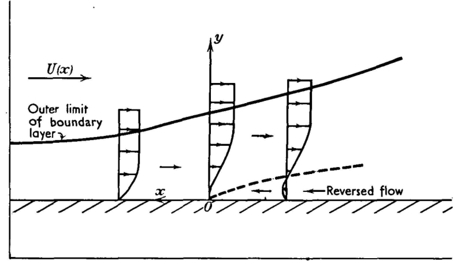
Figure 1: Onset and continuation past separation, [St58]

Mathematically, boundary layer separation has been characterized in the work of [DM15]. We point the reader also to the works [SWZ19] as well as the paper [E00] in which a separation result is announced. Separation occurs at a point $x_{\ast}$ (which in Figure 1 corresponds to $x_{\ast}=0$) if $\partial_{y}u_{P}(x_{\ast},0)=0$, while $\partial_{y}u_{P}(x,0)>0$ for $x<x_{\ast}$.

In the present work, we are concerned with describing the solution after separation, that is, to the right of $x=0$ in Figure 1. Physically, the flow after separation undergoes a new phenomenon of reversal and recirculation: the tangential velocity can be negative, compared to the “pre-separation" regime. Mathematically, the fact that $u_{P}$ changes sign completely destroys the pre-existing approaches to the stationary Prandtl equations (for example [DM15], [OS99], [Ser66], [Iy19], [SWZ19]), which, as we have described above, is to regard the equations as an evolution. In this work, we introduce an entirely new framework to study the Prandtl system in this reversal regime.

The problem of continuing the solution to (LABEL:eq:PR:0) after the Goldstein singularity has historically garnered significant attention from many fluid-dynamicists:

“A famous paper by Goldstein asserts that… the solution of the boundary layer equations can, in general, not be continued beyond the point of separation. Subsequent attempts by many authors to overcome the difficulty of continuation have failed." (P. Lagerstrom, 1975, [Lag75])

Several features become clear upon inspection: since the flow after separation exhibits reversal flow, there exist regions where $u_{P}<0$ (below the dotted curve in Figure 1), and also regions where $u_{P}>0$ (above the dotted curve in Figure 1). In particular, the assumption that $u_{P}\geq 0$ is not true, and the classical point of view of regarding (LABEL:eq:PR:0) as a forward evolution in $x$ completely breaks down.

We develop a new framework, and introduce a new point of view to study the solution in this reversal regime. We devote Section 2 to describing this new point of view, the steps of our proof, and the various difficulties that are encountered. As a result, we only briefly mention here some aspects of our point of view in a relatively informal manner. The dotted line in Figure 1 which emerges immediately after the Goldstein singularity occurs depicts the set $\{u_{P}=0\}$. We identify this curve as a free-boundary which needs to be characterized. Above this free boundary, we have $u_{P}>0$, and therefore (LABEL:eq:PR:0), in principle, should behave like a forward evolution equation in $x$. Below this free boundary, $u_{P}<0$, and therefore (LABEL:eq:PR:0), in principle, should behave as a backwards evolution in $x$. For this reason, we will regard the reversal problem as a mixed-type problem: the equation changes type across $\{u_{P}=0\}$ from forward to backward parabolic. It is useful to keep the following picture, Figure 2, in mind.

Figure 2: Prandtl as a Free Boundary Mixed-Type Problem

In general, mixed-type problems are those in which the equation undergoes a change of type across a particular hypersurface. Some classical examples of mixed-type equations include the Tricomi equation, $u_{xx}+xu_{yy}=0$, and the Keldysh equation, $xu_{xx}+u_{yy}=0$. Evidently, these two aforementioned equations change type from elliptic (when $x>0$) to hyperbolic (when $x<0$) across the hypersurface $\{x=0\}$. Linear mixed-type problems have been studied in the past, though certainly not as intensively as their elliptic/ parabolic/ hyperbolic counterparts. The methods surrounding these problems are largely dependent on deriving explicit solutions, see for instance the book of Bitsadze, [Bit64], for a relatively comprehensive overview of linear methods.

In contrast, quasilinear mixed-type problems pose substantial difficulties, and there are exceedingly few results. The two equations mentioned above have become increasingly important in gas dynamics recently due to their appearance in problems related to transonic shock formation and the shock reflection problem. We refer the reader to some excellent works in this direction: the pioneering works of Morawetz, for example [Mor04], as well as the remarkable works of Chen-Feldman: [CF03], [CF10] (again, to name just a few).

It appears to be a general principle that quasilinear, mixed-type problems may be regarded as a free-boundary problem. Indeed, if we return to the Tricomi equation and replaced it with $u_{xx}+f(u)u_{yy}=0$, then $f(u)$ is playing the role of $x$, and we would need to determine the zero set $f(u)=0$ in order to determine the hypersurface across which the equation changes type. This turns out to be extremely challenging in general, which is one reason why there are so few results regarding quasilinear, mixed-type problems.

In the present work, due to the sign change of the coefficient of $u(x,y)$ in front of the $\partial_{x}u$ term, our situation is a quasilinear, mixed type problem which results in the formation of a free boundary, $\{u=0\}$, whose characterization is a main goal. This free-boundary point of view is novel for the stationary Prandtl system. A further complexity is that the term $v\partial_{y}u$ in (LABEL:eq:PR:0) is nonlocal in the vertical direction due to the incompressibility, which has the potential of spoiling this mixed-type characterization.

We urge the reader to consult Figure 3 which depicts these three (3) flows of information. Above the free boundary, $\{u=0\}$, the coefficient $u>0$, and we expect forward parabolic behavior (information flows left-to-right). Below the free boundary, the coefficient $u<0$ and we therefore expect backward parabolic behavior (information flows right-to-left). The nonlocal term, $v\partial_{y}u$, sends information from bottom-to-top through the incompressibility $v=-\int_{0}^{y}\partial_{x}u$. Obtaining efficient ways to disentangle these three (3) types of information flow is extremely challenging, delicate, and is a central achievement of this paper.

Figure 3: Flow of Information in the Prandtl system

It is worth mentioning that a second reason for the lack of works contending with quasilinear mixed-type problems is simply that, at least as far as we are aware, it is relatively rare to find a physically natural context in which these arise, at least compared to their classical hyperbolic, parabolic, elliptic counterparts (again, the well-studied transonic shock problem from gas dynamics is a notable exception). A noteworthy aspect of our present work even at the outset is that we encounter a natural setting, from the point of view of fluid dynamics, which presents as a quasilinear, mixed-type problem.

We note that our setup, Figure 2, is also reminiscent of the classical Obstacle problem or the Stefan problem, but with some key differences. In the Obstacle problem or Stefan problem, one regards the set $\partial\{u=0\}$ as a “free boundary", whose regularity is the crucial question of study. On the other hand, the setup differs from ours as typically an elliptic or parabolic equation (for instance, $\Delta u=0$ or $\partial_{t}u-\Delta u=0$) is prescribed only in the region $\{u>0\}$, and the equation is not allowed to become of mixed-type. We refer the reader to the many classical works in this area, for instance [Caf77], [FRS20], [FS17] just to name a few. There is also a large literature on the related porous medium equation, which also features a degeneracy in the diffusion. Nearly all results we know of regarding the free-boundary porous medium equation require the degeneracy coefficient to remain nonnegative; see for example [BFR18], and the many references therein.

1.2 Self-Similarity and Reversal

For concreteness, we shall fix the Euler flow in (1.3) to be the following

$$u_{E}(x):=x^{n},\qquad n=\frac{\beta}{2-\beta},\qquad-0.2<\beta<0.$$ (1.4)

This choice of $u_{E}(x)$ and corresponding forcing $-\partial_{x}p_{E}(x)$ into (LABEL:eq:PR:0) is known to produce a self-similar reversed solution to the Prandtl equations. Indeed, consider the ansatz:

$$u_{FS}(x,y):=u_{E}(x)f^{\prime}(\eta),\qquad\eta:=\frac{y}{x^{\frac{1-n}{2}}}.$$ (1.5)

The self-similar profile, $f(\cdot)$, satisfies the following equation:

$$f^{\prime\prime\prime}+ff^{\prime\prime}+\beta(1-(f^{\prime})^{2})=0,\qquad f(0)=f^{\prime}(0)=0,\qquad f^{\prime}(\infty)=1,$$ (1.6)

which is often referred to as a Falkner-Skan self-similar profile to the Prandtl equations. Numerical simulations for negative values of $\beta$ yield the following right-most profile shown below, which undergoes reversed flow (see for instance, [L20], P. 35):

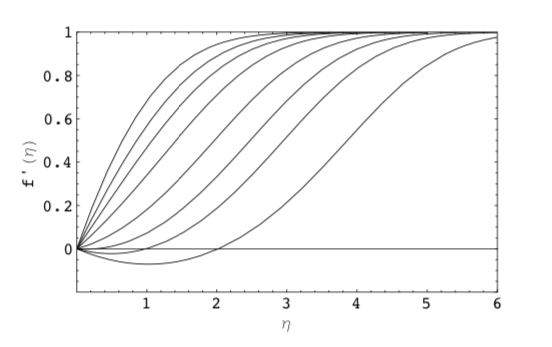
Figure 4: Self Similar Falkner-Skan Profiles

As far as mathematical treatments of these self-similar flows, we state the following classical result:

Lemma 1.1 (Stewartson, [St54]).

For $\beta_{\ast}<\beta<0$, where $\beta_{\ast}<0$, there exists a solution $f(\eta)$ whose graph of $f^{\prime}$ undergoes “reversal", that is, $f^{\prime\prime}(0)<0$, $f^{\prime}(\eta)\leq 0$ for $0\leq\eta\leq\eta_{\ast}$, and $f^{\prime}(\eta)>0$ for $\eta_{\ast}<\eta<\infty$.

After the work [St54], the quantification of the largest negative value $\beta_{\ast}$ for which one can find reversed self-similar Falkner-Skan (“FS") profiles has been a subject of study, [BS66], [H72], [YL13], for instance. As discussed in the works [Har37], [St54], [BS66], these “reversed" self-similar profiles are classical in the boundary layer theory due to their importance in connection with boundary layer separation, and also their importance in various applied settings (such as airfoil design in aerodynamics, etc…).

Our main objectives in this work are to establish the existence of an open set of data that results in reversed (non self-similar) flows, and to provide stability theorems: if data is prescribed “near" these reversed Falkner-Skan profiles, they remain “near" them on an order one tangential scale.

Remark 1.2.

Our choice of the “FS" profiles is exclusively for the sake of concreteness: they serve as a particular solution to the Prandtl equations (LABEL:eq:PR:0) (of course, with adverse pressure gradient), which exhibit reversed flow. One could repeat our results for a much wider class of reversed flows.

1.3 Prescribed Data and Main Result

To our knowledge, all prior mathematical results on (LABEL:eq:PR:0) fall into one of two categories: (1) construction and analysis of specific self-similar solutions (for instance [Go49], [St54], [YL13]), or (2) studying the wellposedness/ finite-$x$-blowup of (LABEL:eq:PR:0) as an initial value problem, with data prescribed at $\{x=0\}$ (for instance, [OS99], [GI18b], [Ser66], [Iy19], [DM15], [SWZ19], [WZ19]). The present work is distinguished since, as described earlier, (LABEL:eq:PR:0) cannot be regarded as a traditional Cauchy problem in the presence of flow reversal.

We thus pose (LABEL:eq:PR:0) with initial and final data, but for appropriate spatial regions. Moreover, the actual region we pose the data on and the precise type of data is a delicate matter, as we will see. This is to be expected if one keeps in mind other mixed-type problems: it is often the case that even posing the right data is part of the problem (the reader can consult the book of [Bit64], for instance). This is especially true in quasilinear mixed-type problems, and in particular we shall see this is the case in the present work.

We first fix a parameter $L>0$ which describes our tangential length scales. Upon doing so, we define $y_{1},y_{2}$ associated to the Falkner-Skan solution, (1.5):

$$u_{FS}(1,y_{1})=f^{\prime}(y_{1})=0,\qquad u_{FS}(1+L,y_{2})=(1+L)^{n}f^{\prime}(\frac{y_{2}}{(1+L)^{\frac{1-n}{2}}})=0$$ (1.7)

We will be looking for solutions perturbed around $u_{FS}$:

$$\psi_{P}=\psi_{FS}+\varepsilon\psi_{R},\qquad u_{P}=u_{FS}+\varepsilon u_{R},\qquad v_{P}=v_{FS}+\varepsilon v_{R},\qquad 0<\varepsilon<<1,$$ (1.8)

where the subscript $``R"$ stands for “Remainder," and $\varepsilon$ is the size of the perturbation. Above, we introduce the stream function $\psi_{P}$ such that $\partial_{y}\psi_{P}=u_{P}$, $-\partial_{x}\psi_{P}=v_{P}$, and $\psi_{P}|_{y=0}=0$.

We also define two versions of the remainder vorticity; the classical vorticity which corresponds to vertical differentiation of the velocity, as well as the “good-unknown" vorticity of Masmoudi-Wong, [MW15], denoted below by $\omega_{g}(x,y)$ (see also [AWXY15]):

$$\omega_{R}(x,y):= \partial_{y}u_{R}(x,y),$$ (1.9)

$$\omega_{g}(x,y):= \omega_{R}(x,y)-\frac{\partial_{y}^{2}u_{FS}(x,y)}{\partial_{y}u_{FS}(x,y)}u_{R}(x,y).$$ (1.10)

It will be on $\omega_{g}$ that we prescribe our data. This is done in order to capitalize on a delicate, new cancellation we discover in this paper which essentially semi-linearizes the Prandtl equations into an Airy-type equation near the interface.

We also define the curve $\Lambda_{G}(x)$ to be the zero set of the background flow, $u_{FS}$, from (1.5), and the free boundary $\Lambda(x)$ to be the perturbed zero set of the full solution, $u_{P}$:

$$u_{FS}(x,\Lambda_{G}(x))=0,\qquad u_{P}(x,\Lambda(x))=u_{FS}(x,\Lambda(x))+\varepsilon u_{R}(x,\Lambda(x))=0$$ (1.11)

It is useful to have the image below, Figure 5, in mind (which is a slightly more detailed version of Figure 2).

Figure 5: $(x,y)$ Domain

As shown in Figure 5, the numbers $y_{1}(\varepsilon),y_{2}$ are defined as follows:

$$y_{1}(\varepsilon)=\Lambda(1),\qquad y_{2}=\Lambda(1+L).$$ (1.12)

Equation (LABEL:eq:PR:0) will thus also be supplemented with initial datum at $x=1$, but only for $y>y_{1}(\varepsilon)$, and backwards initial datum at $x=1+L$, but only for $0<y\leq y_{2}$:

$$\omega_{g}|_{x=1}(y)= F_{Left}\Big{(}\frac{1}{L^{\frac{1}{3}}}(\frac{y}{y_{1}(\varepsilon)}-1)\Big{)}\qquad y>y_{1}(\varepsilon),$$ (1.13a)

$$\omega_{g}|_{x=1+L}= F_{Right}\Big{(}\frac{1}{L^{\frac{1}{3}}}(\frac{y}{y_{2}}-1)\Big{)},\qquad 0\leq y\leq y_{2},$$ (1.13b)

We note that the normalizations above by $y_{1}(\varepsilon),y_{2}$ enable us to think of the given data, $F_{Left}(\cdot)$, $F_{Right}(\cdot)$ as “profile" functions. $F_{Left}(\cdot)$ will be defined on $1\leq z\leq\infty$ and $F_{Right}(\cdot)$ will be defined on $0\leq z\leq 1$. We also note that on the right, prescribing $\omega_{g}$ is equivalent to prescribing $u$ itself (by integrating vertically). This is however not the case on the left.

Several points are noteworthy about the setup:

• Nonresonant tangential scales: The tangential length-scale we choose will need to be non-resonant. As we state in the main theorem below, there exist discretely many values $0<L_{1}<L_{2}<\dots<L_{Max}$ which we need to avoid in choosing our tangential domain $x\in(0,L)$. These discrete resonant values correspond to the presence of zero eigenvalues for a particular elliptic operator we derive and study, and depend only on the choice of background flow, $u_{FS}$. Understanding the physical interpretation of these resonances is an interesting question for further investigation.

• Data in a product space: As we can see from (1.13a), (1.13b), we prescribe two functions. One is to initiate the forward evolution, above the free boundary, and the second is to initiate the backward evolution, below the free boundary. To make this precise, we introduce the product space

  $$\mathcal{P}_{general}:=\{(F_{Left},F_{Right})| F_{Left}:\mathbb{R}_{+}\mapsto\mathbb{R},F_{Right}:\mathbb{R}_{-}\mapsto\mathbb{R},$$

  $$\text{supp}(F_{Right})\subset(-y_{b},0),\|(F_{Left},F_{Right})\|_{\mathcal{P}_{general}}<\infty\},$$ (1.14)

  where

  $$\|(F_{Left},F_{Right})\|_{\mathcal{P}_{general}}:=\sum_{j=0}^{J_{Max}}\|\partial_{\zeta}^{j}F_{Left}\langle\zeta\rangle^{3M_{Max}}\|_{L^{\infty}(\mathbb{R}_{+})}+\sum_{j=0}^{J_{Max}}\|\partial_{\zeta}^{j}F_{Right}\|_{L^{\infty}(\mathbb{R}_{-})}$$ (1.15)

  Above, the parameters $M_{Max},J_{Max}$ could in principle be optimized, but we choose to leave then as generic large numbers. We note that prescribing decay of $F_{Left}(\cdot)$ guarantees implicitly that $u_{R}(x,\cdot)$ decays at $y\rightarrow\infty$. This will be established rigorously by the calculation (1.17). This property on $u_{R}$ is then preserved by the equation for all $x\in(1,1+L)$. We also note that $F_{Right}$ is a function defined on $\mathbb{R}_{-}$ (as opposed to on a bounded interval). The parameter $y_{b}$ will be chosen concretely by $y_{b}=\frac{1}{2}\min\{1,L^{-\frac{1}{3}}\}$. This guarantees, according to (1.13b), that $\omega_{g}$ is also compactly supported away from $y=0$.

• Prescribing the “good-unknown" vorticity: We have made a choice to prescribe $\omega_{g}$, defined in (1.10), on both sides, as opposed to the velocity, $u$, itself as one typically prescribes for the classical Prandtl equation in the sign definite setting $u_{P}\geq 0$. This is to capitalize on a delicate, completely new, structure we discover for the stationary Prandtl equations: it is $\omega_{g}$ that undergoes a “change of type", not $u$ itself. Indeed, when one considers the term $v_{P}\partial_{y}u_{P}=(-\int_{0}^{y}\partial_{x}u_{P})\partial_{y}u_{P}$ in (LABEL:eq:PR:0), it is completely non-obvious and non-trivial to see how this transport term influences the “mixed-type" point-of-view we have developed thus far.

  In this paper, we introduce a new Crocco-type transformation that effectively rewrites (LABEL:eq:PR:0) as a “mixed-type" problem for the good-unknown $\omega_{g}$, up to lower order terms that we treat perturbatively. The cancellations used for this transformation have not been utilized before in the study of the stationary Prandtl equation, and draw an interesting connection with techniques used in the unsteady Prandtl setting ([MW15], [AWXY15]). In particular, this new structure we discover motivates the choice of prescribing $\omega_{g}$ on both sides.

• The velocity $u$ at $\{x=1\}$: There is an asymmetry created by the non-locality in the equations (the term $v_{P}\partial_{y}u_{P})$. On the right, due to the boundary condition $u|_{y=0}=0$, we can express $u$ itself at $x=1+L$ in terms of an integral operator on $F_{Right}$. Letting $u(1+L,y)=G_{Right}(\frac{y}{y_{2}})$, we can integrate to find

  $$G_{Right}(z)=\overline{u_{FS}}^{\prime}(1,z)\int_{0}^{z}\frac{F_{Right}(L^{-\frac{1}{3}}(z^{\prime}-1))}{\overline{u_{FS}}^{\prime}(1,z^{\prime})}\,\mathrm{d}z^{\prime}.$$ (1.16)

  On the left, the situation is different. In order to recover the velocity $u$ at $x=1$, one needs two pieces of information: the profile $F_{Left}(\cdot)$ and the unknown, normalized, quantity $\boldsymbol{\mu}_{1}[y_{1}(\varepsilon)]:=\frac{y_{1}(\varepsilon)-y_{1}}{\varepsilon}$, which represents the deviation between the blue and red dots in Figure 5. Indeed, a small calculation shows that $u(1,y)=G_{Left}(\frac{y}{y_{1}(\varepsilon)})$, where the profile $G_{Left}(\cdot):[1,\infty)\mapsto\mathbb{R}$ is given by

  $$G_{Left}(z):=\boldsymbol{\mu}_{1}[y_{1}(\varepsilon)]\overline{u_{FS}}^{\prime}(1,z)+\overline{u_{FS}}^{\prime}(1,z)\int_{1}^{z}\frac{F_{Left}(L^{-\frac{1}{3}}(z^{\prime}-1))}{\overline{u_{FS}}^{\prime}(1,z^{\prime})}\,\mathrm{d}z^{\prime},$$ (1.17)

  where above, the $\overline{u_{FS}}(1,z)$ are the “profile versions" of $u_{FS}$: $\overline{u_{FS}}(1,z):=u_{FS}(\lambda_{G}(1)z)$.

  The interpretation of this calculation is that we cannot prescribe $u$ on both sides. Instead we must leave the projection $\boldsymbol{\mu}_{1}[y_{1}(\varepsilon)]$ onto the one-dimensional subspace spanned by $\overline{u_{FS}}^{\prime}(1,\cdot)$ on the left as free. This projection is determined through the global behavior of the solution. This is a major departure from all prior works on the stationary Prandtl equation, and display the extremely subtle nature of studying the Prandtl system in the reversed regime.

• Nonlinearly shifted vertical scale: We have defined $y_{1}(\varepsilon)$ to be a nonlinear correction to the known $y_{1}$: it is given by $y_{1}(\varepsilon)=\Lambda(1)$. One subtlety, therefore, is that we can prescribe the profile function $F_{Left}(\cdot)$ as data, but then we need to shift the argument according to (1.13a).

  Remark 1.3.

  We could have alternatively provided this data in the translated form $G_{left}(y-y_{1}(\varepsilon))$, again for a profile function $G_{Left}:[0,\infty)\mapsto\mathbb{R}$. We chose to give it in the quotient form (1.13a) out of convenience, as this form translates well in our $z$ variable (see for instance, (3.19d)).

We need standard compatibility conditions and smoothness conditions on the function, $u_{R}(1+L,\cdot)$, which we define here:

$$u_{R}(1+L,y_{2})=0,\qquad\partial_{y}^{j}u_{R}(1+L,0)=0,\qquad j=2,3.$$ (1.18)

These will be enforced through a mean condition on $F_{Right}$:

$$\int_{0}^{1}\frac{F_{Right}(L^{-\frac{1}{3}}(z^{\prime}-1))}{\overline{u_{FS}}^{\prime}(1,z^{\prime})}\,\mathrm{d}z^{\prime}=0,$$ (1.19)

and enables us to fix $y_{2}$ in (5).

For ease of exposition, while our proof carries over easily to data in $\mathcal{P}_{general}$ introduced in (1.14), we choose to work with

$$\mathcal{P}= C^{\infty}_{c}(\overline{\mathbb{R}_{+}})\times C^{\infty}_{c}(\overline{\mathbb{R}_{+}}).$$ (1.20)

We will also introduce some subspaces of $\mathcal{P}$. First, we introduce functions which are compactly supported away from $0$:

$$\widehat{\mathcal{P}}:=C^{\infty}_{c}(\mathbb{R}_{+})\times C^{\infty}_{c}(\mathbb{R}_{+})$$ (1.21)

Second, we introduce

$$\bar{\mathcal{P}}_{k_{\ast}}:=\{(\widehat{F}_{Left},\widehat{F}_{Right})\in\widehat{P}:\ell_{0}^{(k)}=0,\ell_{1}^{(k)}=0\text{ for }1\leq k\leq k_{\ast}\},$$ (1.22)

where $\ell_{0}^{(k)},\ell_{1}^{(k)}$ will be linear functionals that can be unspecified for now.

We first state a special case of our main result (which we choose to state as a theorem in its own right so that we can refer to it in the body of the paper):

Theorem 1.4 (Small $L$ Version).

Let $0<L<<1$ relative to universal constants. Fix any $(F_{Left},\\ F_{Right})\in\mathcal{P}$ such that (1.19) holds, and take $\omega_{g}$ to achieve the data as shown in (1.13a) - (1.13b). There exist sufficiently large numbers $M_{Max},J_{Max},$ and $k_{\ast}$ depending only on universal constants such that the following holds. There exists $\varepsilon_{\ast}$ such that $0<\varepsilon_{\ast}<<L$ such that for any $0<\varepsilon<\varepsilon_{\ast}$, we have the a-priori stability estimates:

$$\sum_{k=0}^{k_{\ast}}\|(L\partial_{x})^{k}\psi_{R}\|_{L^{\infty}_{z}L^{6}_{x}}+\|(L\partial_{x})^{k}u_{R}\|_{L^{\infty}_{z}L^{6}_{x}}+\|(L\partial_{x})^{k}\omega_{R}\|_{L^{\infty}_{z}L^{6}_{x}}\leq o_{L}(1)\|F_{Left},F_{Right}\|_{\mathcal{P}},$$ (1.23)

for solutions $\omega_{g}\in H^{k_{\ast}}_{x}(0,1;H^{1}_{y})$.

The above result is “stability" in the normal sense in the boundary layer theory: by prescribing $F_{Left},F_{Right}$ for the perturbations, the smallness is assumed at the boundaries, $\{x=1,y\geq y_{1}(\varepsilon)\}\cup\{x=1+L,y\leq y_{2}\}$, and proven to persist on the interior of the domain. Many steps in the analysis of this paper are devoted to the proof of Theorem 1.4. As a result, for the majority of the paper, with the exception of Section 11, we will be under the hypothesis of Theorem 1.4.

Remark 1.5.

Retaining the $o_{L}(1)$ dependence on the $\|\cdot\|_{\mathcal{P}}$ norm will not be relevant for this paper, but it will be convenient to retain this dependence for our companion paper, [IM22b].

The most general result we have is the following:

Theorem 1.6 (Nonresonant $L$ Version).

Fix any $(F_{Left},F_{Right})\in\mathcal{P}$ such that (1.19) holds, and take $\omega_{g}$ to achieve the data as shown in (1.13a) - (1.13b). Let the maximal tangential length scale $L_{Max}>0$ be any fixed number. There exist a discrete set of resonant lengths, $\{L_{k}\}_{k=1}^{N}$, $0<L_{k}<L_{k+1}<L_{Max}$, depending only on the background profile, $u_{FS}$, and numbers $M_{Max},J_{Max},$ and $k_{\ast}$, depending only on universal constants such that the following holds. Choose $L\in(0,L_{Max})\setminus\cup_{k=1}^{N}L_{k}$. There exists an $\varepsilon_{\ast}>0$, small relative to $\min_{k}|L-L_{k}|$ such that for any $0<\varepsilon<\varepsilon_{\ast}$, we have the a-priori stability estimates:

$$\sum_{k=0}^{k_{\ast}}\|(L\partial_{x})^{k}\psi_{R}\|_{L^{\infty}_{y}L^{6}_{x}}+\|(L\partial_{x})^{k}u_{R}\|_{L^{\infty}_{y}L^{6}_{x}}+\|(L\partial_{x})^{k}\omega_{R}\|_{L^{\infty}_{y}L^{6}_{x}}\lesssim \|F_{Left},F_{Right}\|_{\mathcal{P}},$$ (1.24)

for solutions $\omega_{g}\in H^{k_{\ast}}_{x}(0,1;H^{1}_{y})$.

We refer the reader to Section 2 in which we provide a detailed overview of the ideas we introduce and the overall strategy we follow to obtain Theorems 1.4 and 1.6.

Both of the above theorems are stability results, assuming the existence of a qualitatively smooth solution, $\omega_{g}\in H^{k_{\ast}}_{x}(0,1;H^{1}_{y})$. Due to the mixed-type nature of the problem, it is not the case that a-priori stability estimates lead immediately to the construction of the solution. Therefore, we have chosen to split our work into two papers. This paper contains the more substantial aspect, namely the a-priori stability estimates.

The argument leading to the construction of the solution is given in a companion paper, [IM22b], which essentially performs an iteration which uses as a “black-box" the stability analysis of this paper (Theorems 1.4, 1.6). The argument in [IM22b] is also in the spirit of the recent work [DMR22] on a related mixed-type problem. We can now state the main result that combines the stability theorems, Theorems 1.4, 1.6, with the existence result of [IM22b]:

Theorem 1.7 (Existence and Stability).

Fix an arbitrary $(\overline{F}_{Left},\overline{F}_{Right})\in\overline{\mathcal{P}}_{k_{\ast}}$, where $k_{\ast}$ is chosen sufficiently large relative to universal constants. There exists an operator $\mathcal{N}_{side}:\overline{\mathcal{P}}_{k_{\ast}}\mapsto\mathcal{P}$, which is a compact perturbation of the identity, such that the following holds. Let $(F_{Left},F_{Right}):=\mathcal{N}_{side}[\overline{F}_{Left},\overline{F}_{Right}]$. Let $L\in(0,L_{Max})\setminus\cup_{k=1}^{N}L_{k}$. There exists an $\varepsilon_{\ast}>0$, small relative to $\min_{k}|L-L_{k}|$ such that for any $0<\varepsilon<\varepsilon_{\ast}$, the following is valid.

• There exists a unique solution $\psi_{R}$ such that $\omega_{g}$ achieves the given data as shown in (1.13a) – (1.13b). Moreover, this solution has the regularity $\partial_{x}^{k}u_{R}\in L^{2}_{x}H^{1}_{y}$ for each $k$, $0\leq k\leq k_{\ast}$.

• The solution obeys the stability estimates

  $$\sum_{k=0}^{k_{\ast}}\|(L\partial_{x})^{k}\psi_{R}\|_{L^{\infty}_{y}L^{6}_{x}}+\|(L\partial_{x})^{k}u_{R}\|_{L^{\infty}_{y}L^{6}_{x}}+\|(L\partial_{x})^{k}\omega_{R}\|_{L^{\infty}_{y}L^{6}_{x}}\leq o_{L}(1)\|\bar{F}_{Left},\bar{F}_{Right}\|_{\bar{\mathcal{P}}_{k_{\ast}}}.$$ (1.25)

• The data on the sides can be described precisely as follows

  $$(F_{L},F_{R})= (\widehat{F}_{L},\widehat{F}_{R})+(Q_{L},Q_{R})$$ (1.26a)

  $$(\widehat{F}_{L},\widehat{F}_{R})= (\bar{F}_{Left},\bar{F}_{Right})+c_{-1}\mathbb{e}_{-1}+\sum_{k=1}^{k_{\ast}}(c_{0}^{(k)}\mathbb{e}^{(k)}_{0}+c^{(k)}_{1}\mathbb{e}^{(k)}_{1})$$ (1.26b)

  $$(Q_{L},Q_{R})= (\chi(\rho)\sum_{k=1}^{k_{\ast}}q_{L,2+3(k-1)}\rho^{2+3(k-1)},\chi(\rho)\sum_{k=1}^{k_{\ast}}q_{R,2+3(k-1)}\rho^{2+3(k-1)})$$ (1.26c)

  where $\chi,\mathbb{e}_{-1},\mathbb{e}_{0}^{(k)},\mathbb{e}_{1}^{(k)}$ are fixed functions, and the $4k_{\ast}+1$ numbers

  $$\mathbb{A}_{k_{\ast}}:=(c_{0}^{(k)},c_{1}^{(k)},c_{-1},q_{L,2+3(k-1)},q_{R,2+3(k-1)})_{k=1}^{k_{\ast}}$$ (1.27)

  are determined by the prescribed functions $(\bar{F}_{Left},\bar{F}_{Right})\in\overline{\mathcal{P}}_{k_{\ast}}$ and obeys the estimate

  $$|\mathbb{A}_{k_{\ast}}|_{\mathbb{R}^{4k_{\ast}+1}}\lesssim o_{L}(1)\|(\bar{F}_{Left},\bar{F}_{Right})\|_{\overline{\mathcal{P}}_{k_{\ast}}}.$$ (1.28)

1.4 Related Literature

The boundary layer theory originated with Prandtl’s seminal 1904 paper, [Pr1904], which developed the theory in precisely the present setting: for 2D, steady flows over a plate. Since its inception, the boundary layer theory has had monumental impacts in various domains of physics and engineering, perhaps most notably in aerodynamics. Despite it being a classical physical theory, mathematical results are less widespread. In fact, in Prandtl’s original work, he states the following:

“The most important practical result of these investigations is that, in certain cases, the flow separates from the surface at a point [$x_{\ast}$] entirely determined by external conditions… As shown by closer consideration, the necessary condition for the separation of the flow is that there should be a pressure increase along the surface in the direction of the flow." (L. Prandtl, 1904, [Pr1904])

The stationary Prandtl equations are a classical system, whose wellposedness theory was initiated by Oleinik in the classical works, [OS99]. Indeed, the dichotomy between favorable and unfavorable pressure gradient (which was actually pointed out in the original work of Prandtl) appears in Oleinik’s results: she obtains local in $x$ wellposedness results in general, and, in the case of favorable pressure gradients, global wellposedness.

The local wellposedness results of Oleinik rely upon a nonlinear change of variables, which faces difficulty upon further differentiation and therefore cannot be employed to obtain higher regularity estimates. Higher regularity was obtained in [GI18a] through energetic arguments, and in [WZ19] using maximum principle type arguments.

In the case of $\partial_{x}p_{E}(x)\leq 0$, the result of Serrin, [Ser66] characterizes the self-similar Falkner-Skan profiles as asymptotic in $x$ “attractors": general solutions to the Prandtl system approach self-similarity as $x\rightarrow\infty$. This result was revisited using different techniques in [Iy19]. While the methods employed by Serrin are maximum principle based, [Iy19] relies more on weighted energy/ virial type estimates.

In the case of $\partial_{x}p_{E}(x)>0$, separation can occur, and we refer to the recent work [DM15] which shows the existence of an open set of datum that undergoes the Goldstein singularity. The methods from [DM15] rely upon making a self-similar change of variables, and subsequently using modulation theory techniques. We refer also to the work [SWZ19], which provides a different, maximum principle based approach to separation.

Regarding flow reversal in the stationary Prandtl equations, several authors have investigated the structure of the self-similar Falkner-Skan profiles, (1.6). This began with classical investigations by Hartree, [Har37], Stewartson, [St54], Brown and Stewartson, [BS66], Hastings, [H72], and there also are some more recent works in this direction: [YL13]. As far as we know, all known results on reversal are regarding the particular self-similar profiles (1.6), which are extremely important from the point of view of applications. Indeed, the reader can consult the discussions in the sources [Har37], [St54], [BS66] which discuss the various applied settings in which the FS profiles are used (airfoil design, etc…). The present paper is the first to consider stability of these profiles.

As stated earlier, we note that due to the mixed-type nature of the problem, it is a nontrivial task to go from a-priori stability estimates to the construction of the solution. This is achieved in our companion work, [IM22b]. We refer the reader also to the recent work of [DMR22] which addresses the existence of strong solutions to the mixed-type problem $u\partial_{x}u-\partial_{y}^{2}u=0$.

There is a separate but very important question of validity of the Prandtl ansatz in describing the inviscid limit of Navier-Stokes. Here, there are very few works in the stationary setting, which are all relatively recent. The first results were local in the tangential variable, for instance [GI18a], [GI18c], and also [GVM18]. Recently, the works [IM20], [IM21] established stability of the Prandtl ansatz globally in the tangential variable with asymptotics in $x$. See also the related works, [GZ20], [GN14].

For unsteady flows, the picture is rather different than the stationary setting, and for which there is a substantial body of works studying both (1) wellposedness results as well as (2) stability results for the inviscid limit of Navier-Stokes. We focus the discussion here only wellposedness results, since the present paper is not concerned with stability under the inviscid limit. For wellposedness results, we refer the reader to [OS99], [AWXY15], [MW15], [KMVW14] assuming either monotonicity or partial monotonicity in Sobolev spaces. If one removes the hypothesis of monotonicity, wellposedness results are in smoother spaces (either analytic or Gevrey spaces): [DiGV18], [GVM15], [KV13],[LMY20], [SC98]. In Sobolev spaces, the unsteady Prandtl equations are illposed: [GVD10]. We refer the reader also to finite time blowup results: [EE97], as well as unsteady boundary layer separation: [CGM18], [CGIM18], [CGM19] using blowup arguments.

The above discussion is not comprehensive, and we have elected to provide a more in-depth of the steady theory due to its relevance to the present paper. We refer to the articles, [BT13], [E00], and references therein for a more complete review of other aspects of the boundary layer theory.

1.5 Notational Conventions

Coordinate Systems We will be working with four coordinate systems in our analysis. The $(x,y)$ coordinates are the original coordinates in which the system (LABEL:eq:PR:0) is set. The $(s,z)$ coordinates are self-similar and adapted to the free-boundary; they are defined in (3.12). The $(s,Y)$ and $(s,Z)$ coordinate systems are local to the “interface", $\{y=\Lambda(x)\}$, and are defined in (3.22) and (3.30), respectively. We denote by $\mathcal{F}$ the usual Fourier transform defined for functions, $f\in L^{2}(\mathbb{R})$:

$$\mathcal{F}[f](\xi)=\widehat{f}(\xi):=\int_{\mathbb{R}}e^{-i\xi s}f(s)\,\mathrm{d}s,$$ (1.29)

and $\mathcal{F}^{-1}$ the inverse Fourier transform.

One Dimensional “Modulation" Variables: We will need to introduce and control several one-dimensional quantities in our analysis. We introduce these quantities here:

Modulation Variables	Defining Relation
$\Lambda(x)$	$u_{FS}(x,\Lambda(x))+\varepsilon u_{R}(x,\Lambda(x))=0$
$\Lambda_{G}(x)$	$u_{FS}(x,\Lambda_{G}(x))=0$
$\Xi(x)$	$\Lambda(x)=\Lambda_{G}(x)+\varepsilon\Xi(x)$
$\lambda(s)$	$=\Lambda(x)$
$\lambda_{G}(s)$	$=\Lambda_{G}(x)$
$\mu(s)$	$=\Xi(x)$
$\gamma^{(j)}_{k,\Omega}(s)$,   $j=1,2,3$	$=\partial_{Z}^{j-1}\Omega_{k}|_{Z=0}(s)$
$\gamma^{(j)}_{k}(s)$,   $j=1,2,3$	$=\partial_{z}^{j}u_{k}|_{z=1}(s)$
$\gamma^{(j)}_{k}(s)$,   $j=-1,0$	$=\partial_{z}^{j+1}\psi_{k}|_{z=1}(s)$

Parameters: The main small parameters that we have are $L$ (only in the course of proving Theorem 1.4), the tangential length scale, and $\varepsilon$, the size of the perturbation (and hence the pre-factor in front of the quadratic terms). We use $o_{L}(1)$ to refer to a quantity $n(L)$ satisfying $\lim_{L\downarrow 0}n(L)=0$.

2 Main New Ideas and Strategy of the Proof

In this section, our aim is two-fold. First, we want to provide an outline of the proof and organize our strategy into the main steps. Second, by doing so, we will be able to highlight the difficulties that arise and the several main ingredients we need to employ in order to obtain our result.

2.1 The Point of View: Mixed-Type, Free Boundary Problem

Our starting point is to cast the problem as a mixed-type, free boundary problem. This is in contrast to the classical point of view on (LABEL:eq:PR:0), which is to regard (LABEL:eq:PR:0) as an evolution equation in the $x$ (tangential) direction. Indeed, viewing (LABEL:eq:PR:0) as an evolution is appropriate when $u_{P}\geq 0$, since $u_{P}$ is the coefficient of the transport $\partial_{x}$. However, as soon as $u_{P}$ is allowed to change signs, as in the reversal regime we are interested in, this logic no longer applies. We are thus forced to completely abandon prior approaches used to study the stationary Prandtl system, and develop a new point of view.

2.1.1 Mixed Type Equation

To form the general approach then, we linearize the left-hand side of (LABEL:eq:PR:0) around $u_{FS}$ via

$$u_{P}=u_{FS}+\varepsilon u_{R},\qquad v_{P}=v_{FS}+\varepsilon v_{R}.$$ (2.1)

This produces, to leading order in $\varepsilon$, the equations

$$u_{FS}\partial_{x}u_{R}+u_{R}\partial_{x}u_{FS}+v_{FS}\partial_{y}u_{R}+v_{R}\partial_{y}u_{FS}-\partial_{y}^{2}u_{R}=0.$$ (2.2)

To simplify the present discussion, we go to the vorticity form of (2.2), and we also drop most of the transport terms so as to only consider:

$$u_{FS}(x,y)\partial_{x}\omega_{R}-\partial_{y}^{2}\omega_{R}=0.$$ (2.3)

We have a rough heuristic that the most challenging aspect of the problem is determined locally near the curve $(x,\Lambda_{G}(x))$, the zeros of $u_{FS}$. It is then natural to introduce a variable,

$$z=\frac{y}{\Lambda_{G}(x)}$$ (2.4)

such that this zero set is expressed as $\{z=1\}$ (this is done precisely, at the nonlinear level, in (3.12)). Since $u_{FS}(x,y)\approx z-1$ near $z=1$, we can then view (2.3) locally near $\{z=1\}$ as approximately behaving like solutions to the following problem (we introduce the shift $Z=z-1$ so as to move the interface from $\{z=1\}$ to $\{Z=0\}$):

$$Z\partial_{x}\omega-\partial_{Z}^{2}\omega=0,\qquad(x,Z)\in(1,1+L)\times\mathbb{R}.$$ (2.5)

We will call (2.5) our first “toy problem". We note that in the proof, the relation between $Z$ and $z$ is more complex than the heuristic version introduced just above.

The equation (2.5) is not globally an evolution in a fixed direction: if $Z>0$, we would regard (2.5) as a forward parabolic equation, whereas if $Z<0$, we would regard (2.5) as a backward parabolic equation. For this reason, we classify (2.5) as “mixed-type". This observation is required for us to even pose the appropriate data for the problem. According to this observation, it is natural to prescribe data on the left only for $Z\geq 0$: $\omega(1,z),Z\geq 0$ and data on the right only for $Z\leq 0$: $\omega(1+L,Z),Z\leq 0$.

2.1.2 Free Boundary Formulation

Returning now to (2.3), the appropriate quasilinear version becomes

$$(u_{FS}(x,y)+\varepsilon u_{R}(x,y))\partial_{x}\omega_{R}-\partial_{y}^{2}\omega_{R}=0.$$ (2.6)

We thus arrive at a general principle which seems to hold in mixed-type problems: the quasilinearity in the transport creates a “free-boundary", $u_{FS}(x,\Lambda(x))+\varepsilon u_{R}(x,\Lambda(x))=0$. The zero set $(x,\Lambda(x))$ depends on the perturbation, $u_{R}$. On the other hand, one needs to know the zero set, $(x,\Lambda(x))$ in order to derive bounds and ultimately solve for the perturbation because this curve is the curve across which the equation changes type. This principle is alluded to in, for instance, [CF03], [CF10].

To see this more quantitatively, we introduce the nonlinear analogue of the $z$ variable from (2.4), as well as the corresponding self-similar tangential rescaling:

$$\frac{\,\mathrm{d}s}{\,\mathrm{d}x}=\frac{1}{\Lambda(x)^{2}},\qquad z=\frac{y}{\Lambda(x)}=\frac{y}{\Lambda_{G}(x)+\varepsilon\Xi(x)},\qquad u_{FS}(x,\Lambda(x))+\varepsilon u_{R}(x,\Lambda(x))=0.$$ (2.7)

Letting $\mu(s)=\Xi(x)$, $u(s,z)=u_{R}(x,y)$, $\bar{u}(s,z)=u_{FS}(x,y)$, $\lambda(s)=\Lambda(x)$, we arrive at our “free-boundary formulation" of (2.6):

$$(\bar{u}+\varepsilon u)\partial_{s}\omega-\partial_{z}^{2}\omega-\varepsilon\mu^{\prime}(s)=F,\qquad(s,z)\in(1,1+\bar{L})\times(0,\infty)$$ (2.8a)

$$\bar{u}(s,\frac{\lambda_{G}(s)+\varepsilon\mu(s)}{\lambda(s)})+\varepsilon u(s,1)=0.$$ (2.8b)

Above, $F$ contains “harmless terms". The interpretation of (2.8a) is that the quantity $\mu(s)$ represents the perturbation of the free boundary. It influences the main vorticity equation through the appearance of $-\varepsilon\mu^{\prime}(s)$ in (2.8a). On the other hand, it is determined through the implicit relation (2.8b).

We can further simplify the heuristics in two ways: first, we can imagine that the main behavior to understand (2.8a) – (2.8b) is “near $z=1$" (which turns out to not be fully true due to the nonlocality of standard parabolic equations). Moreover, we can Taylor expand (2.8b) around $\frac{\lambda_{G}(s)}{\lambda(s)}$, which is the zero set of $\bar{u}$ itself. This produces the new, toy problem (to make symmetric the problem, we again introduce the shifted variable $Z=z-1$):

$$Z\partial_{s}\omega-\partial_{Z}^{2}\omega-\varepsilon\mu^{\prime}(s)=F,\qquad(s,Z)\in(1,1+\bar{L})\times\mathbb{R}$$ (2.9a)

$$\mu(s)=-\frac{\lambda(s)}{\bar{u}_{z}(s,\frac{\lambda_{G}(s)}{\lambda(s)})}u(s,1),\qquad s\in(1,1+\bar{L})$$ (2.9b)

$$\omega|_{s=1}(Z)=\omega_{Left}(Z),Z>0\qquad\omega|_{s=1+\bar{L}}(Z)=\omega_{Right}(Z),\qquad Z<0.$$ (2.9c)

We note by homogenizing $\omega_{Left},\omega_{Right}$ and creating a new forcing $F$ (depending only on the data), we can, without loss of generality, assume $\omega_{Left}=\omega_{Right}=0$. The system (2.9b) – (2.9c) now informs a few of our forthcoming steps. Notice that $\mu(s)$, the perturbation to the free boundary, is determined by taking the trace of $u(s,1)$.

2.2 New Transformations and Cancellations in the Prandtl System

A starting point for the study of (2.8b) – (2.9c) is to set $\varepsilon=0$, which reads as follows:

$$Z\partial_{s}\omega-\partial_{Z}^{2}\omega=F,\qquad(s,Z)\in(1,1+\bar{L})\times\mathbb{R}$$ (2.10a)

$$\omega|_{s=1}(Z)=0,\qquad Z>0,\qquad\omega|_{s=1+\bar{L}}=0,\qquad Z<0.$$ (2.10b)

It is a standard fact that the stationary Prandtl equations are nonlocal due to the term $v\partial_{y}u$. One can ask: how does the nonlocality interact (and potentially disturb) the mixed-type behavior we anticipate? Thus far, we have ignored the nonlocal term by considering the simplification (2.3). In order to characterize and handle this nonlocality, we will introduce several new formulations of the stationary Prandtl equations. These new structures we introduce and take advantage of are completely new for the stationary Prandtl equation.

2.2.1 Local Transformations: A new perspective on Crocco and Masmoudi-Wong

One of our main steps of the analysis will be through exploiting specific features of the Airy functions, solutions to the ODE (A.1), which can only be done if our system of study is exactly of the form (2.10a), up to lower order terms or terms containing a prefactor of $\varepsilon$. The motivation for invoking these Airy functions will be explained in the next subsection, Section 2.3. For now, we turn to the task of transforming (2.2) into (2.10a).

An inspection of (2.2) indicates that the nonlocal term $v_{R}\partial_{y}u_{FS}$ provides a serious obstacle to obtaining exactly (2.10a). One way to mitigate the effect of the non-local term is by going to the vorticity form. Indeed, a standard cancellation shows

$$\bar{w}\partial_{s}u+v\partial_{z}\bar{u}-\partial_{z}^{2}u=0$$ (2.11a)

$$\bar{w}\partial_{s}\omega+v\partial_{z}^{2}\bar{u}-\partial_{z}^{2}\omega=0$$ (2.11b)

Thus, while the non-local term appears at equal level of regularity with the “Airy" part in (2.11a), we see that there is a gain in $\partial_{z}\approx\partial_{s}^{\frac{1}{3}}$ in (2.11b).

Nevertheless, we want to study the effect of this term in a precise manner. Again localizing to near the zero set of $\bar{w}$, we can introduce the change of variables and change of function:

$$Y=\bar{w},\qquad\phi(s,Y)=\psi(s,z),\qquad V(s,Y):=\partial_{Y}^{2}\phi(s,Y).$$ (2.12)

Considering now the equation on $\phi$, we see an even more substantial cancellation:

$$Y\partial_{s}V-|\bar{w}_{z}|^{2}\partial_{Y}^{2}V=\text{lower order terms}.$$ (2.13)

Thus, the non-locality is, in a sense, eliminated through the change of variables, (2.12).

From (2.13), we would now like to eliminate the term $\bar{w}_{z}^{2}$ in front of the diffusion. We achieve this by splitting the diffusion coefficient into $\bar{w}_{z}^{2}-\bar{w}_{z}^{2}(s,1)$, which we move to the right-hand side and subsequently use the vanishing, and $\bar{w}_{z}^{2}(s,1)$, which is purely dependent on $s$. To do this, we introduce another transformation, which is a simple rescaling, $Z=p(s,Y)=\frac{Y}{\bar{w}_{z}(s,1)^{\frac{2}{3}}}$. This process is carried out in Section 3.4. We then set $\Omega(s,Z)=V(s,Y)$.

To appreciate further the introduction of $V(s,Y)$ and $\Omega(s,Z)$ in (2.12), we can compute an explicit representation of $\Omega$ which turns out to read

$$\Omega(s,Z)=\frac{1}{\bar{w}_{z}^{2}}(\partial_{z}u-\frac{\bar{w}_{zz}}{\bar{w}_{z}}u)=\omega_{g}$$ (2.14)

which is reminiscent of (1) the classical Crocco-transform as well as (2) the good-unknown of Masmoudi-Wong, [MW15]. To our knowledge, neither of these ideas have been used in the study of the stationary Prandtl equation. In this work, we will need to use these ideas extensively. Moreover, our method of performing these well-chosen transformations appears to be a completely new perspective on the Masmoudi-Wong good unknown.

2.2.2 von-Mise type good unknowns

The $(s,Y)$ coordinates introduced in (2.12) (and by implication, the $(s,Z)$ coordinate system introduced thereafter) are only defined locally near the interface, $\{z=1\}$. This is due to the definition $Y=\bar{w}$, where $\partial_{z}\bar{w}$ degenerates as $z\rightarrow\infty$ and also in the interior of $0<z<1$. Since our analysis is not localized to just near $\{z=1\}$, but needs to eventually extend globally to $0<z<\infty$, we need a different set of transformations which apply globally in $z$ (in particular in the “outer region").

In this region, our formulation of the system in the self-similar variables, $(s,z)$, reads:

$$\bar{w}\partial_{s}u+v\partial_{z}\bar{w}-\partial_{z}^{2}u=F,$$ (2.15a)

$$\bar{u}(s,\frac{\lambda_{G}(s)+\varepsilon\mu(s)}{\lambda(s)})+\varepsilon u(s,1)=0,$$ (2.15b)

We observe the presence of the nonlocal term $v\partial_{z}\bar{w}$. By noticing that $v=-\partial_{s}\psi$, and $\partial_{s}\mu\approx\partial_{s}u(s,1)$ according to (2.15b), we identify this term as being transported, and therefore losing one $s$-derivative if moved to the right-hand side and treated perturbatively. To handle this, we introduce the quantity

$$U:=\bar{w}^{2}\partial_{z}\Big{(}\frac{\psi}{\bar{w}}\Big{)}.$$ (2.16)

The quantity $U$ is reminiscent of the classical von-Mise type unknown, which has been used in various works prior to this one (see, for instance, [Iy19], [IM20], [IM21], [DM15] as just a few examples).

2.2.3 Three Regions: “von-Mise" $\mapsto$ “Crocco" $\mapsto$ “von-Mise"

The discussion above indicates that there are three regions: a “Crocco" region localized to the interface, where we use the good unknown $\Omega$ (reminiscent of the Crocco transform), and two “von-Mise" regions where we use the good unknown $U$: one which is localized below the interface and the other above the interface. Therefore, we have the following diagram, Figure 6, which is useful to keep in mind.

Figure 6: Three Regions

Prior works on the stationary Prandtl system, [DM15], [OS99], [Iy19], [Ser66] essentially relied exclusively on a globally defined “von-Mise" region, where one can work with $U$ and go back and forth to $u$ and $\psi$. This is due to the sign definite, $u_{P}\geq 0$, property in all these prior works. Here, such a strategy will fail due to the sign change of the background flow. It is for this reason that we need to decompose and work with both the von-Mise and Crocco formulations, depending on the value of $z$.

When performing estimates, we need to proceed “upwards". Indeed, near the physical boundary $y=0$, one has a sign condition $\bar{u}_{FS}\leq 0$, and therefore, we can work with the von-Mise unknown $U$ (and invert to $u$ and $\psi$). However, as we approach the interface, we need to switch to the Crocco variable ($\omega_{g}$), which due to the sign condition $\bar{w}_{z}\gtrsim 1$ in the interface region, is well-defined and invertible. As we then leave the interface towards $z\rightarrow\infty$, the Crocco transform starts to fail (due to the rapid vanishing of $\bar{w}_{z}$ as $z\rightarrow\infty$) and the von-Mise formulation becomes valid again.

2.3 Airy Analysis

2.3.1 Dirichlet-Neumann Matching

It will turn out that the main quantity of interest in solving (2.9c) – (2.10a) is the one-dimensional quantity

$$\Omega|_{Z=0}(s)=:\gamma_{1}(s),\qquad 1<s<1+\bar{L}.$$ (2.17)

First of all, to see that $\gamma_{1}(s)$ is, in a sense, the “main unknown", notice that if we knew $\gamma_{1}(s)$, then (2.10a) – (2.10b) would totally decouple into an “upper" problem $(z>0)$ in which a forward parabolic evolution would take place and into a “lower" problem $(z<0)$ in which a backwards parabolic evolution would take place.

In order to identify the unknown trace $\gamma_{1}(s)$, our strategy is a “Dirichlet-to-Neumann" matching procedure. Indeed, consider the following maps:

$$\gamma_{1}(s)\mapsto\Omega^{(\pm)}(s,Z),\qquad Z>0\mapsto\gamma^{(\pm)}_{2}[\gamma_{1}](s):=\partial_{Z}\Omega^{(\pm)}(s,0),$$

where we think of the Neumann condition, $\gamma^{(\pm)}_{2}[\cdot]$ as a functional on $\gamma_{1}$. Above, we have $(+)$ corresponding to the Neumann condition arising from the “upper" solution ($Z>0$) and similarly the $(-)$ corresponding to the Neumann condition arising from the “lower" solution ($Z<0$). We now can realize $\gamma_{1}(s)$ as the unique solution to the equation:

$$\gamma_{2}^{(+)}[\gamma_{1}]=\gamma_{2}^{(-)}[\gamma_{1}].$$ (2.18)

2.3.2 The maps $\gamma_{2}^{\pm}[\cdot]$

Now that we have identified (2.18) as a central object of study, we need to characterize the maps $\gamma_{2}^{(\pm)}[\cdot]$. By symmetry, let us only deal with $\gamma_{2}^{(+)}[\cdot]$. Upon passing to the $\Omega$ quantity and the $Z$ variable, our system reads

$$Z\partial_{s}\Omega-\partial_{Z}^{2}\Omega=F,\qquad(s,Z)\in(1,1+\bar{L})\times\mathbb{R}_{+},$$ (2.19a)

$$\omega|_{s=1}=0,$$ (2.19b)

$$\omega|_{z=0}=\gamma_{1}(s).$$ (2.19c)

Above, $F$ contains lower order terms that depend on $\Omega$ as well as the stream function $\psi$. One way to understand solutions to (2.19a) – (2.19c) is to (1) take extensions in $s$ to $s\in\mathbb{R}$ (there is some care to be taken in doing this), and subsequently (2) taking the Fourier transform in the $s$ variable. Doing so results in:

$$i\xi Z\widehat{\Omega}-\partial_{Z}^{2}\widehat{\Omega}=\widehat{F},\qquad(\xi,z)\in\mathbb{R}\times\mathbb{R}_{+},$$ (2.20a)

$$\widehat{\omega}|_{Z=0}=\widehat{\gamma_{1}}(\xi).$$ (2.20b)

We can now explicitly describe solutions to (2.20a) – (2.20b) through the Airy functions (and the phase-shifted Airy functions):

$$\widehat{\Omega}^{(+)}(\xi,Z)= \frac{ai((i\xi)^{\frac{1}{3}}Z)}{ai(0)}\widehat{\gamma}_{1}(\xi)+\mathcal{G}^{(+)}[F],$$ (2.21a)

$$\widehat{\Omega}^{(-)}(\xi,Z)= \frac{B_{-sgn(\xi)}((i\xi)^{\frac{1}{3}}Z)}{B_{-sgn(\xi)}(0)}\widehat{\gamma}_{1}(\xi)+\mathcal{G}^{(-)}[F]$$ (2.21b)

Above, the quantity $\mathcal{G}^{(\pm)}[\cdot]$ is a functional on the source term, $F$, and should be regarded temporarily as being on the right-hand side. We note here that the solution in the region $z<0$ needs to be described in two cases, due to the asymptotic behavior of the Airy functions in different subsets of $\mathbb{C}$. The quantities $ai(\cdot),B_{\pm}(\cdot)$ are the classical Airy function and appropriate phase shifted Airy functions, as described in Lemma A.1. To explain this more, we refer the reader to Figure 7.

Figure 7: Dirichlet-Neumann Matching on $\mathbb{C}$

First of all, the three sectors $\Sigma_{0},\Sigma_{+1},\Sigma_{-1}$ are defined so that there is a consistent choice of decaying Airy basis function on each sector. However, as the sector changes, the decaying basis function also changes. Lemma A.1 details this, but in summary: the decaying basis function in $\Sigma_{0}$ is $ai(\cdot)$, in $\Sigma_{+1}$ is the phase shifted $B_{+1}(\cdot):=ai(e^{-\frac{2}{3}\pi i}\cdot)$, and in $\Sigma_{-1}$ is the phase shifted $B_{-1}(\cdot):=ai(e^{\frac{2}{3}\pi i}\cdot)$.

Let us first turn to the case when $Z>0$, where we write the solution as (2.21a). The arguments into the Airy functions are of the form $(i\xi)^{\frac{1}{3}}Z$, which for $Z>0$, $\xi>0$, are elements on the ray $\arg=\frac{\pi}{6}$. For reasons to be described shortly, we think of these rays as parametrized by $Z$, for fixed $\xi$. Similarly, complex numbers $(i\xi)^{\frac{1}{3}}Z$ when $Z>0$ and $\xi<0$ are elements of the ray $\arg=-\frac{\pi}{6}$. Both of these rays remain within $\Sigma_{0}$, and therefore we choose $ai((\xi)^{\frac{1}{3}}Z)$ independently of $sgn(\xi)$, as in (2.21a).

When $Z<0$, the situation is different. Indeed, when $Z<0$ and $\xi>0$, we have $\arg((i\xi)^{\frac{1}{3}}Z)=-\frac{5\pi}{6}$, and this ray (parametrized by $Z$ for fixed $\xi$ is contained in $\Sigma_{-1}$). On the other hand, when $Z<0$ and $\xi<0$, we have $\arg((i\xi)^{\frac{1}{3}}Z)=\frac{5\pi}{6}$, and this ray is contained in $\Sigma_{+1}$. Therefore, we need to distinguish the two cases by $sgn(\xi)$ in (2.21b). We will see that these are crucial observations: they lead to the “hidden ellipticity" in the problem, as we describe now.

2.3.3 Hidden Ellipticity on the Boundary and the Fractional Poisson Problem

We now turn to (2.18). Given Figure 7, we can reinterpret the Dirichlet-Neumann matching of (2.18) as matching the derivative of $ai(\cdot)$ along the ray $\arg=\frac{\pi}{6}$ with the derivative of $B_{-1}(\cdot)$ along the ray $\arg=-\frac{5\pi}{6}$ at the origin, for $\xi>0$. Similarly, for $\xi<0$, we can think of matching the derivative of $ai(\cdot)$ along the ray $\arg=-\frac{\pi}{6}$ with the derivative of $B_{+1}(\cdot)$ along the ray $\arg=\frac{5\pi}{6}$ again at the origin (since we are interested in the Neumann condition at $Z=0$).

Performing this calculation with (2.21a) – (2.21b) gives roughly the identity:

$$(i\xi)^{\frac{1}{3}}\Big{(}\frac{ai^{\prime}(0)}{ai(0)}-\frac{B_{-sgn(\xi)}^{\prime}(0)}{B_{-sgn(\xi)}(0)}\Big{)}\widehat{\gamma}_{1}(\xi)=\text{Source Terms depending only on $F$}.$$ (2.22)

Examining now the structure of the “Wronskian"-type Fourier multiplier appearing above, we discover the explicit identity (this is done in Lemma 5.3):

$$\frac{ai^{\prime}(0)}{ai(0)}-\frac{B_{-sgn(\xi)}^{\prime}(0)}{B_{-sgn(\xi)}(0)}=\frac{1}{ai(0)^{2}}\frac{1}{2\pi}e^{-isgn(\xi)\frac{\pi}{6}}.$$ (2.23)

The fact that we distinguished the dependance of the basis functions on $sgn(\xi)$ in (2.21b) produces the $\xi$-dependent factor above in (2.23). Pairing now with the prefactor of $(i\xi)^{\frac{1}{3}}$ appearing in (2.22), we discover a “hidden-ellipticity":

$$(i\xi)^{\frac{1}{3}}\Big{(}\frac{ai^{\prime}(0)}{ai(0)}-\frac{B_{-sgn(\xi)}^{\prime}(0)}{B_{-sgn(\xi)}(0)}\Big{)}\widehat{\gamma}_{1}(\xi)=\frac{1}{ai(0)^{2}}\frac{1}{2\pi}|\xi|^{\frac{1}{3}}\widehat{\gamma}_{1}(\xi).$$ (2.24)

The multiplier being applied to $\gamma_{1}(\xi)$ is a fractional Laplacian. This “hidden-ellipticity" reflects the fact that the free boundary, described by $\widehat{\gamma}_{1}(\xi)$ should by symmetric between the left and the right side. Multipliers of the type $(i\xi)^{\frac{1}{3}}$ are directional, whereas multipliers of $|\xi|^{\frac{1}{3}}$ are symmetric.

Recalling the boundary conditions of $\gamma_{1}(1)=\gamma_{1}(1+\bar{L})=0$, we thus naturally arrive at a fractional elliptic problem:

$$(-\Delta_{D})^{\frac{1}{6}}\gamma_{1}=\mathcal{G}^{(+)}[F]-\mathcal{G}^{(-)}[F],\qquad s\in(1,1+\bar{L}),$$ (2.25a)

$$\gamma_{1}|_{(1,1+\bar{L})^{C}}=0,$$ (2.25b)

$$\mathcal{G}^{(+)}[F]\approx\int_{0}^{\infty}ai((i\xi)^{\frac{1}{3}}z)\widehat{F}(\xi,z)\,\mathrm{d}z.$$ (2.25c)

Above, the fractional Laplacian is the classical Riesz fractional Laplacian of power $1/6$:

$$(-\Delta_{D})^{\frac{1}{6}}u(s):=\mathcal{R}_{(1,1+\bar{L})}\mathcal{F}^{-1}|\xi|^{\frac{1}{3}}\mathcal{F}u.$$ (2.26)

Several remarks are in order regarding (2.25a) – (2.25b):

First, the scaling (2.19c) – (2.20b) reflects the fact that, formally, $\partial_{s}^{\frac{1}{3}}\approx\partial_{z}$, and the Neumann trace should thus be $1/3$ $s$-derivative weaker than the Dirichlet trace. Second, one can see formally that the operator $\mathcal{G}^{(\pm)}[F]$, defined in (2.25c) are smoothing of order $1/3$ in $s$-derivative. Hence, (2.25a) continues to reflect the fact that the left-hand side of (2.19c) formally gains $\partial_{z}^{2}\approx\partial_{s}^{\frac{2}{3}}$ over the right-hand side. Third, we note that the natural boundary condition for fractional Laplacian operators are exterior conditions, such as (2.25b), which is guaranteed to hold by our method of extensions.

Finally, we find it interesting (but also, a-posteiori natural) that there is some hidden ellipticity in the problem that we need to find and use. Intuitively, this answers the question: if we give data on the left at ($s=1$) and on the right $(s=1+\bar{L})$, how do they “know of, and adapt to, each other’s presence" dynamically? Clearly, the mechanism cannot be purely through independent forward and backwards evolutions. Ellipticity in the tangential, $s$, direction perfectly “factors in" the left and right in a symmetric fashion. Returning to the analogue of Figure 5, we have in the $(s,z)$ coordinates the figure shown below, Figure 8.

Figure 8: $(s,z)$ Domain

Above, the source term $f=f(s)$ is a nonlocal integral operator that depends on the given data $F_{Left},F_{Right}$, as well as lower order terms on the interface itself, $\gamma_{1}$. Therefore, we can write $f=f[F_{Left},F_{Right},\gamma_{1}]$. These lower order terms are what require us to remove certain “resonances" in the parameter, $L$.

2.3.4 Incompressibility and the Codimension Two Decomposition for $\psi$

We return to Figure 3, where the incompressibility condition sends information upwards. One of the primary objectives throughout the analysis is to efficiently disentangle the “upward flow of information" from the forward and backward behavior due to the mixed-type nature of the system. To see the mechanism at play, we recall the map which takes $\Omega$ to $\psi$, for $z>1$:

$$\psi=\underbrace{\gamma^{(-1)}(s)}_{\text{Energy}}+\underbrace{\gamma^{(0)}(s)}_{\text{Energy}}\bar{w}+\underbrace{\bar{w}^{\prime}\int_{1}^{z}\frac{\Omega}{\bar{w}^{\prime}}}_{\text{Airy}}.$$ (2.27)

This inversion formula indicates precisely how we achieve this “untangling" of information flow. The quantity $\Omega$, as we have seen, is determined through the Airy-type analysis, for which the forward-backward dynamic is prominent, and the non-local effects are small.

This leaves the two projections $\gamma^{(-1)}(s)$ and $\gamma^{(0)}(s)$ as undetermined. In contrast, these two projections are determined through a more global information: the physical boundary conditions $u|_{z=0}=\psi|_{z=0}=0$. To actually implement this strategy, we need to proceed as shown in Figure 6: integration vertically from $z=0$, successively passing through a “von-Mise" region, a “Crocco" region, and a third “von-Mise" region. This strategy will be followed in several calculations throughout the proof, see for instance all of Section 4.2, as well as estimate (10.33).

2.4 The $\mathcal{I}$ norm: new Airy-type singular integral bounds

2.4.1 Singular Integral Operators with Airy kernels I

Starting from (2.25a) – (2.25c), it is natural that we need to estimate Fourier integral operators of the type (2.25c). It will turn out to be advantageous in our whole scheme of closing estimates to work in $L^{p}_{s}(1,1+\bar{L})$ spaces, where $p>2$. We choose $p=\frac{5}{2}$ for a concrete choice. The fact that we need to work in $L^{p}$ spaces for $p>2$ as opposed to just $L^{2}$ is to satisfy requirements arising from the energy estimate aspect of the proof, which is discussed in Section 2.5.1.

Given 2.25c, we are motivated to study operators of the type:

$$T[F](s)=\int_{\mathbb{R}}\int_{0}^{\infty}K_{Z}(s-t)F(t,Z)\,\mathrm{d}Z\,\mathrm{d}t,$$ (2.28)

where the kernel above is defined via

$$K_{Z}(x):=\int_{\mathbb{R}}e^{i\xi x}(i\xi)^{\frac{1}{3}}ai((i\xi)^{\frac{1}{3}}Z)\,\mathrm{d}\xi.$$ (2.29)

Our aim becomes to prove $L^{p}_{s}L^{q}_{z}\mapsto L^{p}_{s}$ bounds for the operator $T[F]$. It appears to be fairly nontrivial to obtain bounds of this type, so we rely upon slighly lossier bounds. These are obtained in Lemmas A.9, A.10.

2.4.2 Singular Integral Operators with Airy kernels II

Our design of the ultimate $Z$ norm in which we close all our bounds include crucially what we call the $\mathcal{I}$ norm (see (4.10) for a precise definition). It turns out in order to derive sharp enough estimates on our $\mathcal{I}$ norm quantities, we need to obtain bounds on bi-parameter version of the singular integral operators described above. These turn out to be far more nontrivial. A Duhamel-type formula results in the following expression for the vorticity on the Fourier side:

$$\widehat{\Omega}(\xi,Z)= \frac{1}{(i\xi)^{\frac{1}{3}}\mathcal{W}[ai,bi]}ai((i\xi)^{\frac{1}{3}}Z)\int_{0}^{Z}bi((i\xi)^{\frac{1}{3}}Z^{\prime})\widehat{F}(\xi,Z^{\prime})\,\mathrm{d}Z^{\prime}$$

$$+\frac{1}{(i\xi)^{\frac{1}{3}}\mathcal{W}[ai,bi]}bi((i\xi)^{\frac{1}{3}}Z)\int_{Z}^{\infty}ai((i\xi)^{\frac{1}{3}}Z^{\prime})\widehat{F}(\xi,Z^{\prime})\,\mathrm{d}Z^{\prime}+\text{easier terms.}$$ (2.30)

The two Duhamel-type operators on the right-hand side motivate the study of the following abstractly defined operators:

$$\mathcal{J}_{1}[F;\alpha,\beta](s,Z):= \int_{\mathbb{R}}\int_{0}^{Z}K^{(1)}_{Z,Z^{\prime}}[\alpha,\beta](s-t)F(t,Z^{\prime})\,\mathrm{d}Z^{\prime}\,\mathrm{d}t,$$ (2.31)

$$\mathcal{J}_{2}[F;\alpha,\beta](s,Z):= \int_{\mathbb{R}}\int_{Z}^{\infty}K^{(2)}_{Z,Z^{\prime}}[\alpha,\beta](s-t)F(t,Z^{\prime})\,\mathrm{d}Z^{\prime}\,\mathrm{d}t,$$ (2.32)

where the kernels above are given by

$$K^{(1)}_{Z,Z^{\prime}}[\alpha,\beta](x):= \int_{\mathbb{R}}e^{i\xi x}\alpha((i\xi)^{\frac{1}{3}}Z)(i\xi)^{\frac{1}{3}}\beta((i\xi)^{\frac{1}{3}}Z^{\prime})\,\mathrm{d}\xi,$$ (2.33)

$$K^{(2)}_{Z,Z^{\prime}}[\alpha,\beta](x):= \int_{\mathbb{R}}e^{i\xi x}\beta((i\xi)^{\frac{1}{3}}Z)(i\xi)^{\frac{1}{3}}\alpha((i\xi)^{\frac{1}{3}}Z^{\prime})\,\mathrm{d}\xi.$$ (2.34)

The $\alpha(\cdot),\beta(\cdot)$ appearing above will be the Airy functions, $(ai,bi)$, and derivatives of these functions.

On these singular integral operators, we are required to prove $L^{\infty}_{Z}L^{p}_{s}\mapsto L^{\infty}_{Z}L^{p}_{s}$ estimates. These, once again, appear to be just out of reach. We therefore settle on establishing certain “lossy" bounds, to be found in Lemmas A.11, A.12.

Let us focus only on $\mathcal{J}_{1}$. Roughly speaking, the complication above arises due to the competing decay of $\alpha(\cdot)$ and the growth of $\beta(\cdot)$. For the Airy functions, it turns out that this decay and growth are critical (after integration the resulting product forms exactly a bounded multiplier). Our harmonic analysis estimates in Lemmas A.11, A.12 exactly reflect this structure of the Airy kernels. Moreover, in Lemma A.13, we prove certain “admissibility bounds" on the Airy functions which are required in order to apply the bounds in Lemmas A.11, A.12, which requires a delicate decomposition of the $(\xi,Z,Z^{\prime})$ parameter space.

2.5 Energy Estimates

We will perform energy estimates to control one aspect of our norm. Indeed, given the Neumann trace, $\omega|_{z=1}=\gamma_{1}(s)$, which is an outcome of solving the Poisson problem (2.25a), we can “lift" to $z$ values away from $z=1$ (the interface). During this process, the “upper" problem ($z>1$) is decoupled from the “lower" problem ($z<1$). Moreover, we split our analysis into “interior energy estimates", which are localized near the interface, $\{z=1\}$, and “outer energy estimates", which are valid in the region $|z-1|>\delta$, for a small, but order one, scale $\delta>0$.

2.5.1 Interior (Crocco type) Energy Estimates

In the interior region, near the interface, $\{z=1\}$, we have access to the $(s,Z)$ coordinate system and the good unknown $\Omega$. Indeed, consider the following toy problem:

$$Z\partial_{s}\Omega-\partial_{Z}^{2}\Omega=F,\qquad(s,Z)\in(1,1+\bar{L})\times\mathbb{R}_{+}$$ (2.35a)

$$\Omega|_{Z=0}=\gamma_{1}(s),\qquad\lim_{Z\rightarrow\infty}\Omega(s,Z)=0,$$ (2.35b)

$$\Omega|_{s=1}=F_{Left}(Z).$$ (2.35c)

The weakest energy estimate that we can get away with turns out to be differentiating once in $Z$ and taking inner product against $Z\partial_{Z}^{2}\Omega$. One sees that this results in, essentially, the energy identity

$$\frac{\partial_{s}}{2}\int_{0}^{\infty}Z^{2}\Omega_{Z}^{2}+\int_{0}^{\infty}Z|\partial_{Z}^{2}\Omega|^{2}\approx-\gamma_{1}(s)\gamma_{3}(s).$$ (2.36)

At least for $s\in(1,1+\bar{L})$, where $\bar{L}<<1$, we see the basic requirement that $\|\gamma_{1}\gamma_{3}\|_{L^{1}_{s}(1,1+\bar{L})}<<1$, which is not guaranteed by the left-hand side of the energy identity above. In order to appeal to our bounds from the Poisson problem (2.25a), we have in particular one basic requirement that $\|\partial_{s}^{\frac{1}{3}}\gamma_{1}\|_{L^{2}(1,1+\bar{L})}$ and $\|\partial_{s}^{-\frac{1}{3}}\gamma_{3}\|_{L^{2}(1,1+\bar{L})}$ are both $<<1$ (there is a manipulation required to bring in appropriate factors of $\partial_{s}^{\frac{1}{3}}$ which we disregard for this discussion). This, in turn, is guaranteed by controlling these two quantities in $L^{p}_{s}$ spaces where $p>2$ (we choose $p=\frac{5}{2}$). In particular, we arrive at a constraint that: our energy estimates require studying (2.25a) and therefore the harmonic analysis bounds from Section 2.4 in $p>2$.

2.5.2 Outer (von-Mise type) Energy Estimates

In the exterior region, we lose access to the $(s,Z)$ coordinate system, and we need to work with the less explicit formulation (2.15a) – (2.15b). The starting point of our strategy to perform energy estimates in the exterior region is to introduce the new good unknown $U$ from (2.16). Given this, we need to design and control several norms which are tailored to the variable $U$ (see, for instance, 4.22). We rely upon several new Hardy type inequalities which allow us to go from $\psi$ to $U$ and vice-versa.

2.6 Maximal Regularity Theory

We will need to trade away $\partial_{x}$ derivative to gain back $\partial_{y}$ derivative. This is useful to control nonlinear terms. Here, we note that since we are propagating control over the scaled derivative $L\partial_{x}$, we can only expect to gain $\partial_{y}$ derivatives with weights of $L$ in front. Moreover, since higher $\partial_{x}$ derivatives are controlled with weaker weights at $y=\infty(z=\infty)$, we need to perform this “trade" in an efficient way. Indeed, invoking too many $\partial_{x}$ derivatives, even though they may be available in our norm, could cost us more $L$ powers and decaying weights at $\infty$. These tradeoffs are carefully accounted for in the design and control of our $E_{Max}$ norm, (4.24).

2.7 Spectral Analysis & Discrete Set of Resonances

Our main result applies not just for $L<<1$ but also for $L$ values away from a discrete set of “resonances". To generalize the result from $0<L<<1$ we use crucially the “hidden ellipticity" we have discovered in (2.25a) – (2.25c). Upon rescaling the tangential variable by $L$ to $t=\frac{s}{L}$, it turns out that a more accurate depiction of the real problem (compared to the simplified version presented in (2.25a) – (2.25c)) is

$$(-\Delta_{D})^{\frac{1}{6}}\gamma_{1}+\mathbb{K}_{L}[\gamma_{1}]=\mathcal{R}\circ(\mathcal{G}^{(+)}[F]-\mathcal{G}^{(-)}[F]),\qquad t\in(0,1),$$ (2.37a)

$$\gamma_{1}|_{(0,1)^{C}}=0,$$ (2.37b)

where above, the operator $\mathbb{K}_{L}$ is a bounded operator $L^{2}(0,1)\mapsto L^{2}(0,1)$. Thus, the $L$ dependence has been moved to the bounded operator $\mathbb{K}_{L}$ in (2.37a), and we think of $L$ as a parameter. We identify that the main issue at the linear level becomes to invert the full operator on the left-hand side of (2.37a). When $0<L<<1$, this is achieved by moving the “potential term", $\mathbb{K}_{L}[\gamma_{1}]$ to the right-hand side and treating it perturbatively. When $L$ is large this is no longer possible.

The main obstacle when $L$ is no longer small becomes the potential existence of a kernel to the operator $(-\Delta_{D})^{\frac{1}{6}}\gamma_{1}+\mathbb{K}_{L}[\gamma_{1}]$. In Section 11, we undertake a study of the spectrum of $(-\Delta_{D})^{\frac{1}{6}}\gamma_{1}+\mathbb{K}_{L}[\gamma_{1}]$. We combine two crucial facts:

• There is no kernel when $0<L<<1$

• The operator $(-\Delta_{D})^{\frac{1}{6}}\gamma_{1}+\mathbb{K}_{L}[\gamma_{1}]$ depends analytically on the parameter $L$ (in a sense to be made precise).

These two facts imply that the set of $L$ where kernel elements could appear are discrete (essentially, it is because a nonzero analytic function can only have discretely many zeros). The physical interpretation of these discrete resonances, $\{L_{k}\}$, is an interesting question.

2.8 Plan of the Paper

Now, we briefly describe the plan of the paper. Roughly speaking, the paper proceeds in the order of the subsections above. Section 3 is devoted to introducing our various changes of variables. Section 4 is devoted to introducing our functional framework: various norms and embedding theorems that we will be using repeatedly.

We now introduce the following scheme of a-priori estimates. We refrain from defining norms carefully at this stage, and we refer the reader to Section 4 for the precise definition of all norms. However, we emphasize that our strategy consists of producing five (5) types of coupled estimates. Moreover, we proceed $k$ by $k$, where $k$ represents an $L$-normalized, tangential differentiation (defined precisely in (3.5)).

Proposition 2.1.

Let $0<L<<1$. Let $\psi_{R}$ be a perturbation to $\psi_{FS}$ as in (1.8), such that the good vorticity $\omega_{g}\in H^{k_{\ast}}_{x}(0,1;H^{1}_{y})$. Then the following a-priori bounds are valid:

$$\|\vec{\widetilde{\gamma}}_{\Omega}\|_{\mathcal{M}_{k}}\lesssim o_{L}(1)\|(\Xi^{(k)}_{Left},\Xi^{(k)}_{Right})\|_{A}+o_{L}(1)\sum_{k^{\prime}=0}^{k}\|\psi\|_{Z_{k^{\prime}}},$$ (Airy Analysis)

$$\|\widetilde{\Omega_{I}}\|_{\mathcal{I}_{k}}\lesssim o_{L}(1)\|(\Xi^{(k)}_{Left},\Xi^{(k)}_{Right})\|_{A}+\|\vec{\widetilde{\gamma}}_{\Omega}\|_{\mathcal{M}_{k}}+o_{L}(1)\sum_{k^{\prime}=0}^{k}\|\psi\|_{Z_{k^{\prime}}} \mathcal{I}$$ ( Norm Analysis)

$$\|\Omega_{I}\|_{X_{I,k}^{(\pm)}}\lesssim \|(\Xi^{(k)}_{\pm})\|_{C}+o_{L}(1)\sum_{k^{\prime}=0}^{k}\|\psi\|_{Z_{k^{\prime}}},$$ (Interior Energy Analysis)

$$\|\psi\|_{X_{O,k}^{(\pm)}}\lesssim \|\zeta^{(k)}_{\pm}\|_{B}+o_{L}(1)\sum_{k^{\prime}=0}^{k}\|\psi\|_{Z_{k^{\prime}}},$$ (Outer Energy Analysis)

$$\|\psi\|_{E_{Max,k}}\lesssim \|\psi\|_{X_{O,k}}+\|\psi\|_{X_{I,k}}+\|\Omega_{I}\|_{\mathcal{I}_{k}}+o_{L}(1)\sum_{k^{\prime}=0}^{k}\|\psi\|_{Z_{k}}.$$ (Maximal Regularity Analysis)

Establishing the five bounds in the above proposition constitute the most difficult parts of our analysis. They are labelled according to the “step" in which we perform the bounds. These five “steps" roughly correspond to the discussions in Sections 2.3 - 2.6, respectively. These five bounds above are then obtained in the five sections, Sections 5 – 9, respectively.

According to (4.25), our $Z_{k}$ norm is the sum of the five norms appearing on the left-hand sides of Proposition 2.1. To close the estimate on our $Z_{k}$ norm, we use crucially that the Airy Analysis bound comes with smallness of $o_{L}(1)$ in front of the term $\sum_{k^{\prime}=0}^{k}\|\psi\|_{Z_{k^{\prime}}}$. Therefore, inserting this into the $\mathcal{I}$ norm bound produces smallness also for $\|\widetilde{\Omega_{I}}\|_{\mathcal{I}_{k}}$. Subsequently, adding together the first four bounds in Proposition 2.1 and substituting into the right-hand side of the $E_{Max}$ estimate then produces our basic $Z_{k}$ norm estimate, which we now record.

Corollary 2.1.

Let $0<L<<1$, where $L$ is small relative to universal constants. The following a-priori bound is valid on the solution $\psi$ to the system (3.19a) – (3.19f):

$$\|(\psi,\Omega_{I})\|_{\mathcal{Z}}\lesssim \sum_{k=0}^{k_{\ast}}\Big{(}o_{L}(1)\|(\Xi^{(k)}_{Left},\Xi^{(k)}_{Right})\|_{A}+\|(\zeta^{(k)}_{Left},\zeta^{(k)}_{Right})\|_{B}+\|(\Xi^{(k)}_{Left},\Xi^{(k)}_{Right})\|_{C}\Big{)}.$$ (2.39)

The quantities $(\Xi^{(k)}_{Left},\Xi^{(k)}_{Right})$, $(\zeta^{(k)}_{Left},\zeta^{(k)}_{Right})$ are quantities restricted to the sides, $s=0,Z>0$ and $s=1,Z<0$. We abuse notation above and put $\Xi_{Left}=\Xi_{+}$, $\Xi_{Right}=\Xi_{-}$, and similarly for $\zeta$. To conclude the proof of the theorem, Section 10 is devoted to analyzing the quantities appearing on the right-hand side. This turns out to be a fairly delicate process due to the “bottom-to-top" nonlocal effect. For a standard parabolic problem, computing the “initial data" for higher order tangential derivatives is straightforward upon invoking the equation. Indeed, one expects that higher-order tangential derivatives can be expressed as a combination of normal derivatives of the prescribed data. In our case, since we are only prescribing $\Omega$, $\psi$ itself needs to be determined through integration. In turn, this creates a dependence of the data for $\psi$ (and therefore for higher order tangential derivatives of $\Omega$) on the solution itself (see, for example, the expressions 10.34). Therefore, the delicate analysis of Section 10 separates out a piece of the boundary data on the sides which is intrinsic (in terms of just $F_{Left},F_{Right}$), and a piece which is depending on the global solution. Moreover, it is crucial for Theorem 1.4 to demonstrate the solution-dependent piece comes with a small factor of $o_{L}(1)$. The conclusion of the analysis of Section 10 are the estimates

$$\|\Xi^{(k)}_{Left},\Xi^{(k)}_{Right}\|_{A}\lesssim \|F_{Left},F_{Right}\|_{\mathcal{P}}+L^{\frac{2}{3}}o_{L}(1)\|\psi\|_{Z_{k-1}}$$ (2.40a)

$$\|\zeta^{(k)}_{Left},\zeta^{(k)}_{Right}\|_{B}\lesssim L^{\frac{1}{6}}\|F_{Left},F_{Right}\|_{\mathcal{P}}+o_{L}(1)\|\psi\|_{Z_{k}}$$ (2.40b)

$$\|\Xi^{(k)}_{Left},\Xi^{(k)}_{Right}\|_{C}\lesssim L^{\frac{1}{6}}\|F_{Left},F_{Right}\|_{\mathcal{P}}+o_{L}(1)\|\psi\|_{Z_{k-1}}.$$ (2.40c)

We insert the estimates (2.40a) – (2.40c) into the estimate (2.39), and again using the smallness of $o_{L}(1)$ appearing in the solution dependent components of (2.40a) – (2.40c). Finally, we have that the $\mathcal{Z}$ norm controls the left-hand side of (1.23), which closes our main a-priori bound, (1.23).

To establish Theorem 1.6, we perform in Section 11 the spectral analysis described above in Section 2.7. Two main propositions are established. The first of these propositions involves formulating a Spectral Condition, defined precisely in Definition 11.1, which implies the main result:

Proposition 2.2 (Spectral Version, Informal Version).

Assume the Spectral Condition in Definition 11.1. Let $0<\varepsilon<<1$. Then the same result of Theorem 1.4 holds.

The second proposition involves verifying the spectral condition at all values of $L$ away from a discrete set of resonances. This analysis requires us to (1) prove $L$-analyticity of appropriately defined operators for $L>L_{0}$ and (2) use that Theorem 1.4 implies already that for $0<L\leq L_{0}<<1$ the absence of a kernel for our elliptic problem. We state this proposition here:

Proposition 2.3.

Fix any $L_{0}>0$. The operator $\mathbb{K}_{L}:L^{2}(0,1)\mapsto L^{2}(0,1)$ appearing in (2.25a) is analytic in the parameter $L$ on the domain $L\in(L_{0},\infty)$. More precisely, the map $L\mapsto\mathbb{K}_{L}$ from $(L_{0},\infty)\mapsto\mathbb{O}$ is an analytic map:

$$\sup_{k}\sup_{L\in(L_{0},\infty)}\frac{1}{C^{k+1}k!}\|\partial_{L}^{k}\mathbb{K}_{L}\|_{\mathbb{O}}<\infty.$$ (2.41)

With Proposition 2.3 in hand, we can deduce the spectral condition required for Proposition 2.2 and hence prove Theorem 1.6 through an analyticity argument which is performed rigorously in Section 11.2.1.

3 Self-Similar Changes of Variables

We start the proof of Theorems 1.4 and 1.6 by performing several changes of variables and transformations.

3.1 The $(x,y)$ variables

We are considering the problem given by (LABEL:eq:PR:0), with data (1.13a) – (1.13b), which reads

$$u_{P}\partial_{x}u_{P}+v_{P}\partial_{y}u_{P}-\partial_{y}^{2}u_{P}=-\partial_{x}p_{E}(x),\qquad(x,y)\in(1,1+L)\times(0,\infty),$$ (3.1a)

$$u_{P}|_{y=0}=0,\qquad u_{P}|_{y\rightarrow\infty}=u_{E}(x).$$ (3.1b)

We consider perturbations of the form

$$u_{P}=u_{FS}+\varepsilon u_{R},\qquad v_{P}=v_{FS}+\varepsilon v_{R},\qquad\Lambda(x)=\Lambda_{G}(x)+\varepsilon\Xi(x),$$ (3.2)

where $\Lambda(x)$ defines the perturbed free boundary (and $\varepsilon\Xi(x)$ the perturbation):

$$u_{P}(x,\Lambda(x))=u_{FS}(x,\Lambda(x))+\varepsilon u_{R}(x,\Lambda(x))=0$$ (3.3)

Expanding around $(u_{FS},v_{FS})$, which is an exact solution of (LABEL:eq:PR:0), we obtain the equation for the perturbation $(u_{R},v_{R})$ via

$$(u_{FS}+\varepsilon u_{R})\partial_{x}u_{R}+u_{R}\partial_{x}u_{FS}+(v_{FS}+\varepsilon v_{R})\partial_{y}u_{R}+v_{R}\partial_{y}u_{FS}-\partial_{y}^{2}u_{R}=0.$$ (3.4)

We will need to differentiate tangentially the system above $k_{\ast}$ times. To do this, we introduce the rescaling

$$\tau:=\frac{x-1}{L}\Rightarrow\partial_{\tau}=L\partial_{x}$$ (3.5)

We now differentiate this equation by applying $\partial_{\tau}^{k}$, and group terms according to order of derivative, which after a long manipulation produces the following form:

$$u_{P}\partial_{x}u_{R,k}+u_{Py}v_{R,k}+\mathbb{C}_{1}\partial_{y}u_{R,k}+\mathbb{C}_{2}u_{R,k}+\mathbb{C}_{3}\psi_{R,k}-\partial_{y}^{2}u_{R,k}=\mathcal{R}_{k},$$ (3.6)

where the coefficients are defined as follows:

$$\mathbb{C}_{1}:= v_{FS}+\varepsilon 1_{k\geq 1}v_{R}$$ (3.7a)

$$\mathbb{C}_{2}:= \partial_{x}u_{FS}+1_{k\geq 1}k\partial_{x}u_{P}+\varepsilon 1_{k\geq 2}\partial_{x}u_{R}$$ (3.7b)

$$\mathbb{C}_{3}:= 1_{k=1}\partial_{xy}u_{FS}+1_{k\geq 2}k\partial_{xy}u_{P},$$ (3.7c)

and where

$$\mathcal{R}_{k}= -1_{k\geq 3}\sum_{k^{\prime}=1}^{k-2}\binom{k}{k^{\prime}}u_{FS,k-k^{\prime}}\partial_{x}u_{R,k^{\prime}}-1_{k\geq 3}\varepsilon\sum_{k^{\prime}=1}^{k-2}\binom{k}{k^{\prime}}u_{R,k-k^{\prime}}\partial_{x}u_{R,k^{\prime}}$$

$$-1_{k\geq 1}\sum_{k^{\prime}=0}^{k-1}u_{R,k^{\prime}}\partial_{x}u_{FS,k-k^{\prime}}-1_{k\geq 1}\sum_{k^{\prime}=0}^{k-1}\binom{k}{k^{\prime}}v_{FS,k-k^{\prime}}\partial_{y}u_{R,k^{\prime}}$$ (3.8)

$$-1_{k\geq 3}\sum_{k^{\prime}=1}^{k-2}\binom{k}{k^{\prime}}v_{R,k^{\prime}}\partial_{y}u_{FS,k-k^{\prime}}-1_{k\geq 3}\varepsilon\sum_{k^{\prime}=1}^{k-2}\binom{k}{k^{\prime}}v_{R,k^{\prime}}\partial_{y}u_{R,k-k^{\prime}}$$ (3.9)

$$-1_{k\geq 2}v_{R}\partial_{xy}u_{FS,k-1}-1_{k\geq 2}u_{FS,k}\partial_{x}u_{R}=:\sum_{i=1}^{8}\mathcal{R}_{k}^{(i)}.$$ (3.10)

Above we have also introduced the notation

$$u_{R,k}(x,y):=\partial_{\tau}^{k}u_{R}(x,y),\qquad v_{R,k}(x,y):=\partial_{\tau}^{k}v_{R}(x,y).$$ (3.11)

Note also at the expense of introducing complicated looking coefficients on the left-hand side of (3.6), we have grouped all the $k$’th order terms on the left, so that only lower order ($k-1$ and below) appear in $\mathcal{R}_{k}$.

3.2 The Modulated $(s,z)$ Coordinates

We now change to self-similar variables, $(s,z)$, via

$$\frac{\,\mathrm{d}s}{\,\mathrm{d}x}=\frac{1}{\Lambda(x)^{2}},\qquad z:=\frac{y}{\Lambda(x)}=\frac{y}{\Lambda_{G}(x)+\varepsilon\Xi(x)}.$$ (3.12)

We now transform our functions to

$$u_{k}(s,z)=u_{R,k}(x,y),\qquad v_{k}(s,z):=-\int_{0}^{z}\partial_{s}u_{k},\qquad\psi_{k}(s,z):=\int_{0}^{z}u_{k}$$ (3.13a)

$$\bar{u}(s,z):=u_{FS}(x,y),\qquad\bar{v}(s,z):=-\int_{0}^{z}\partial_{s}\bar{u},\qquad\bar{\psi}(s,z):=\int_{0}^{z}\bar{u}$$ (3.13b)

$$\lambda(s):=\Lambda(x),\qquad\lambda_{G}(s):=\Lambda_{G}(x),\qquad\mu(s):=\Xi(x).$$ (3.13c)

We also define the notation:

$$u_{P}(x,y)=u_{FS}(x,y)+\varepsilon u_{R}(x,y)=\bar{u}(s,z)+\varepsilon u(s,z)=\bar{w}(s,z),$$ (3.14)

to stand for the total background profile.

Associated to (3.12), we record the following identity for a generic function $f=f(s,z)$,

$$\partial_{x}f(s,z)=\frac{1}{\lambda(s)^{2}}\partial_{s}f-\frac{\lambda^{\prime}(s)}{\lambda(s)^{3}}z\partial_{z}f$$ (3.15)

We now write the system for $(u,v)$ in the $(s,z)$ coordinates, which after repeated application of the chain rule (3.15) to (3.4) results in

$$\bar{w}\partial_{s}u_{k}-\partial_{z}\bar{w}\partial_{s}\psi_{k}+\mathcal{A}[\overline{\psi},\psi_{k}]-\partial_{z}^{2}u_{k}=\lambda^{2}\mathcal{R}_{k},\qquad(s,z)\in(1,1+\bar{L})\times(0,\infty).$$

where $\mathcal{R}_{k}$ has been defined in (3.10) Above, we have put $\bar{L}:=\int_{1}^{1+L}\frac{1}{\Lambda(x)^{2}}\,\mathrm{d}x$. We note that $|\bar{L}|\leq L\sup_{x\in(1,1+L)}\frac{1}{\Lambda(x)^{2}}\lesssim L$. We will of course need to ensure the condition that $u_{P}(x,\Lambda(x))=0$, which reads in the $(s,z)$ coordinates

$$\bar{u}(s,\frac{\lambda_{G}(s)+\varepsilon\mu(s)}{\lambda(s)})+\varepsilon u(s,1)=0.$$ (3.16)

We define the following operators to compactify the notation:

$$\mathcal{A}[\psi_{k}]:= \mathbb{c}_{1}\partial_{z}u_{k}+\mathbb{c}_{2}u_{k}+\mathbb{c}_{3}\psi_{k},$$ (3.17)

with coefficients

$$\mathbb{c}_{1}:= \mathbb{C}_{1}(x,y)-\frac{\lambda^{\prime}}{\lambda}\bar{w}z-1_{k=0}\varepsilon\frac{\lambda^{\prime}}{\lambda}\psi$$ (3.18a)

$$\mathbb{c}_{2}:= \mathbb{C}_{2}(x,y)+\frac{\lambda^{\prime}}{\lambda}z\bar{w}_{z}$$ (3.18b)

$$\mathbb{c}_{3}:= \mathbb{C}_{3}(x,y)-\frac{\lambda^{\prime}}{\lambda}\bar{w}_{z}1_{k\geq 1}-\frac{\lambda^{\prime}}{\lambda}\bar{u}_{z}1_{k=0}$$ (3.18c)

The closed, coupled, system for $(u,v,\mu(s))$ then reads:

$$\bar{w}\partial_{s}u_{k}+v_{k}\partial_{z}\bar{w}-\partial_{z}^{2}u_{k}+\mathcal{A}[\psi_{k}]=\lambda^{2}\mathcal{R}_{k},\qquad(s,z)\in(1,1+\bar{L})\times(0,\infty),$$ (3.19a)

$$\bar{u}(x,\frac{\lambda_{G}(s)+\varepsilon\mu(s)}{\lambda(s)})+\varepsilon u(s,1)=0,\qquad s\in(1,1+\bar{L})$$ (3.19b)

$$v(s,z)=-\int_{0}^{z}\partial_{s}u(s,z^{\prime})\,\mathrm{d}z^{\prime}$$ (3.19c)

$$(u_{z}-\frac{\bar{w}_{zz}}{\bar{w}_{z}}u)|_{s=1}=F_{Left}(z),\qquad z>1,$$ (3.19d)

$$(u_{z}-\frac{\bar{w}_{zz}}{\bar{w}_{z}}u)|_{s=1+L}=F_{Right}(z),\qquad 0\leq z\leq 1,$$ (3.19e)

$$u|_{z=0}=u|_{z\rightarrow\infty}=0.$$ (3.19f)

First, we note that due to the compatibility condition (1.18), we have the identities

$$\lambda(1)=\lambda_{G}(1)=y_{1},\qquad\lambda(2)=\lambda_{G}(2)=y_{2},$$ (3.20)

which immediately result in $(1,y_{1})\mapsto(1,1)$ and $(2,y_{2})\mapsto(2,1)$, and moreover, $\{x=1,y\geq y_{1}\}\mapsto\{s=1,z\geq 1\}$ and $\{x=1+L,y\leq y_{2}\}\mapsto\{s=1+\bar{L},z\geq 1\}$. It is for this reason the data on the sides (3.19d) – (3.19e) is obtained from the given data $F_{left},F_{right}$.

We note that, to first order in $\varepsilon$, we can expand the equation (3.19b) at the point $z=\frac{\lambda_{G}(s)}{\lambda(s)}$, using that $\bar{u}(s,\frac{\lambda_{G}}{\lambda})=0$, to obtain

$$0= \bar{u}(s,\frac{\lambda_{G}(s)}{\lambda(s)}+\varepsilon\frac{\mu(s)}{\lambda(s)})+\varepsilon u(s,1)=\bar{u}(s,\frac{\lambda_{G}(s)}{\lambda(s)})+\varepsilon\bar{u}_{z}(s,\frac{\lambda_{G}}{\lambda})\frac{\mu(s)}{\lambda(s)}+\varepsilon u(s,1)+O(\varepsilon^{2}),$$ (3.21)

which yields $\mu(s)=-\frac{\lambda(s)}{\bar{u}_{z}(s,\frac{\lambda_{G}(s)}{\lambda(s)})}u(s,1)$. We note that the pre-factor is signed: $-\frac{\lambda(s)}{\bar{u}_{z}(s,\frac{\lambda_{G}(s)}{\lambda(s)})}<0$. This calculation will be turned into a precise estimate in Lemma 4.12, where we control rigorously the $O(\varepsilon^{2})$ terms appearing in (3.21).

3.3 Straightening the Background: the $Y$ variable

Much of our analysis will take place near the interface $\{z=1\}$. Due to the structure of $\bar{w}$ near $\{z=1\}$, we may perform further changes of variables which are valid only in a thin vertical strip around $\{z=1\}$, which simplify the structure of our system. Indeed, for the remaining changes of coordinates, we will assume that $\delta_{1}$ is chosen such that $u_{FS}^{\prime}\geq\frac{1}{2}u_{FS}^{\prime}(x,\Lambda_{G}(x))>0$ (this quantity is $x$-independent) when $|y-\Lambda_{G}(x)|<\delta_{1}$. Define

$$Y:=\bar{w}(s,z),\qquad\phi_{k}(s,Y):=\psi_{k}(s,z)$$ (3.22)

We now compute the equation (3.19a) on the function $\phi_{k}$, which results in

$$Y\partial_{sY}\phi_{k}-\partial_{s}\phi_{k}-\bar{w}_{z}^{2}\partial_{Y}^{3}\phi_{k}= (\bar{w}\bar{w}_{s}-3\bar{w}_{zz}+\mathbb{c}_{1}\bar{w}_{z})\partial_{Y}^{2}\phi_{k}$$ (3.23)

$$+\Big{(}\frac{\bar{w}\bar{w}_{sz}-\bar{w}_{s}\bar{w}_{z}-\bar{w}_{zzz}+\mathbb{c}_{2}\bar{w}_{z}+\mathbb{c}_{1}\partial_{z}^{2}\bar{w}}{\bar{w}_{z}}\Big{)}\partial_{Y}\phi_{k}+\frac{\mathbb{c}_{3}}{\bar{w}_{z}}\phi_{k}+\frac{\mathcal{R}_{k}}{\bar{w}_{z}}.$$

Due to the fact that the map $(s,z)\mapsto(s,Y)$ defined by (3.22) is only invertible when $\bar{w}_{z}>0$, we will only be performing this change of variables (and hence considering the formulation (3.23)) in a thin strip around $Y=0$.

We introduce now the vorticity in the straightened coordinates, $(s,Y)$:

$$V_{k}(s,Y):=\partial_{Y}^{2}\phi_{k}(s,Y).$$ (3.24)

Differentiating equation (3.23), we obtain the following system on $V$:

$$Y\partial_{s}V_{k}-|\bar{w}_{z}|^{2}\partial_{Y}^{2}V_{k}= \underline{\tau_{1}}\partial_{Y}V_{k}+\underline{\tau_{0}}V_{k}+\underline{\tau_{-1}}\partial_{Y}\phi_{k}+\underline{\tau_{-2}}\phi_{k}+\frac{\partial_{z}}{\bar{w}_{z}}\Big{(}\frac{\mathcal{R}_{k}}{\bar{w}_{z}}\Big{)}.$$ (3.25)

Above, the coefficients are indexed according to $Y$ regularity in $V$. They are defined are follows:

$$\underline{\tau_{1}}(s,Y):= \bar{w}\bar{w}_{s}+\mathbb{c}_{1}\bar{w}_{z}-\bar{w}_{zz},$$ (3.26a)

$$\underline{\tau_{0}}(s,Y):= \frac{\partial_{z}}{\bar{w}_{z}}(\bar{w}\bar{w}_{s}+\mathbb{c}_{1}\bar{w}_{z}-\bar{w}_{zz})+\frac{1}{\bar{w}_{z}}(\bar{w}\bar{w}_{sz}-\bar{w}_{s}\bar{w}_{z}+\mathbb{c}_{2}\bar{w}_{z}+\mathbb{c}_{1}\bar{w}_{zz}-\bar{w}_{zzz})$$ (3.26b)

$$\underline{\tau_{-1}}(s,Y):= \frac{\partial_{z}}{\bar{w}_{z}}\Big{(}\frac{\bar{w}\bar{w}_{sz}-\bar{w}_{s}\bar{w}_{z}-\bar{w}_{zzz}+\mathbb{c}_{2}\bar{w}_{z}+\mathbb{c}_{1}\bar{w}_{zz}}{\bar{w}_{z}}\Big{)}+\frac{\mathbb{c}_{3}}{\bar{w}_{z}},$$ (3.26c)

$$\underline{\tau_{-2}}(s,Y):= \frac{\partial_{z}}{\bar{w}_{z}}\Big{(}\frac{\mathbb{c}_{3}}{\bar{w}_{z}}\Big{)}.$$ (3.26d)

We also record the following identity, which shows the connection between our $(s,Y)$ coordinate system and good unknown, $V(s,Y)$, and the Masmoudi-Wong good-unknown, [MW15]. Indeed, computing using (3.22) and (3.24), we get the identities

$$u_{k}(s,z)=\bar{w}_{z}(s,z)\partial_{Y}\phi_{k}(s,Y),$$ (3.27)

$$\partial_{z}u_{k}(s,z)=\bar{w}_{zz}\partial_{Y}\phi_{k}+\bar{w}_{z}^{2}V_{k}(s,Z)=\frac{\bar{w}_{zz}}{\bar{w}_{z}}u_{k}+\bar{w}_{z}^{2}V_{k},$$ (3.28)

which upon rearranging, results in

$$V_{k}(s,Y)=\frac{1}{\bar{w}_{z}^{2}}(\partial_{z}u_{k}-\frac{\bar{w}_{zz}}{\bar{w}_{z}}u_{k}),$$ (3.29)

which is essentially equivalent to the Masmoudi-Wong good unknown. We find our new perspective on this good unknown noteworthy.

3.4 Eikonal Equation for the $Z$ Variable

Our aim is to now perform a further change of variables, $(s,Y)\mapsto(s,Z)$, which converts the prefactor of $\bar{w}_{z}^{2}$ in front of the diffusion in (3.36) into a constant prefactor of $1$ (as opposed to a nonconstant function of $s$) when restricted to $Y=0$ (coinciding with $Z=0$). We introduce

$$V_{k}(s,Y)=\Omega_{k}(s,Z)=\Omega_{k}(s,p(s,Y)),\qquad Z=p(s,Y).$$ (3.30)

Note that this is a change of variable and function we use only at the vorticity level, unlike the introduction of the $Y$ variable in (3.22), which occurs at the level of the stream function. We also note that, putting (3.30) together with (3.29), we get

$$\Omega_{k}(s,Z)=V_{k}(s,Y)=\frac{1}{\bar{w}_{z}^{2}}(\partial_{z}u_{k}-\frac{\bar{w}_{zz}}{\bar{w}_{z}}u_{k}).$$ (3.31)

We will also introduce a notation for the stream function in $(s,Z)$ coordinates:

$$\Phi_{k}(s,Z)=\phi_{k}(s,Y)$$ (3.32)

Notice while $\partial_{Y}^{2}\phi_{k}=V_{k}$, a more complicated Biot-Savart law relates $\Phi_{k}$ and $\Omega_{k}$:

$$\Omega_{k}(s,Z)=|p_{Y}|^{2}\partial_{Z}^{2}\Phi_{k}+p_{YY}\partial_{Z}\Phi_{k}.$$ (3.33)

We choose the function $p(s,Y)$ explicitly via

$$p(s,Y)=\frac{Y}{\bar{w}_{z}(s,0)^{\frac{2}{3}}}.$$ (3.34)

We record the following identities from an application of the chain rule,

$$Y\partial_{s}V_{k}= Y\partial_{s}\Omega_{k}+Yp_{s}\partial_{Y}\Omega_{k}$$ (3.35a)

$$\partial_{Y}V_{k}= p_{Y}\partial_{Z}\Omega_{k},$$ (3.35b)

$$\partial_{Y}^{2}V_{k}= p_{Y}^{2}\partial_{Z}^{2}\Omega_{k}+p_{YY}\partial_{Z}\Omega_{k}.$$ (3.35c)

From here, we obtain upon invoking (3.34)

$$Y\partial_{s}V_{k}-|\bar{W}^{\prime}|^{2}\partial_{Y}^{2}V_{k}= Z\bar{w}_{z}(s,0)^{\frac{2}{3}}\partial_{s}\Omega_{k}-\frac{\bar{w}_{z}^{2}}{\bar{w}_{z}(s,0)^{\frac{4}{3}}}\partial_{Z}^{2}\Omega_{k}+(p_{Y}^{2}|\bar{w}_{z}|^{2}Zp_{s})\partial_{Z}\Omega_{k}.$$

We therefore observe that the left-hand side of (3.36) is conjugated to a pure Airy operator in the $(s,Z)$ variable, up to lower order terms. Indeed, equation (3.25) in the $(s,Y)$ coordinates transforms into

$$Z\partial_{s}\Omega_{k}-\partial_{Z}^{2}\Omega_{k}=\tau_{2}\partial_{Z}^{2}\Omega_{k}+\tau_{1}\partial_{Z}\Omega_{k}+\tau_{0}\Omega_{k}+\tau_{-1}\partial_{Z}\Phi_{k}+\tau_{-2}\Phi_{k}+\mathbb{F}_{k},$$ (3.36a)

$$\Omega_{k}(1,Z)=\Omega_{k,Left}\Big{(}\frac{Z}{\overline{L}^{\frac{1}{3}}}\Big{)},\qquad Z>0$$ (3.36b)

$$\Omega_{k}(1+\overline{L},Z)=\Omega_{k,Right}\Big{(}\frac{Z}{\overline{L}^{\frac{1}{3}}}\Big{)},\qquad Z<0$$ (3.36c)

Above, we have defined the following quantities:

$$\tau_{2}(s,Z):= \frac{\bar{w}_{z}^{2}}{\bar{w}_{z}(s,0)^{2}}$$ (3.37a)

$$\tau_{1}(s,Z):= -\frac{2}{3}\frac{\bar{w}_{z}^{2}\bar{w}_{sz}(s,0)}{\bar{w}_{z}(s,0)^{\frac{11}{3}}}Z+\frac{\underline{\tau}_{1}}{\bar{w}_{z}(s,0)^{\frac{4}{3}}},$$ (3.37b)

$$\tau_{0}(s,Z):= \frac{\underline{\tau}_{0}}{\bar{w}_{z}(s,0)^{\frac{2}{3}}}$$ (3.37c)

$$\tau_{-1}(s,Z):= \frac{\underline{\tau}_{-1}}{\bar{w}_{z}(s,0)^{\frac{4}{3}}}$$ (3.37d)

$$\tau_{-2}(s,Z):= \frac{\underline{\tau}_{-2}}{\bar{w}_{z}(s,0)^{\frac{2}{3}}}$$ (3.37e)

Finally, we define

$$\mathbb{F}_{k}(s,Z):= \frac{\partial_{z}}{\bar{w}_{z}}\Big{(}\frac{\mathcal{R}_{k}}{\bar{w}_{z}}\Big{)}(s,z).$$ (3.38)

3.5 Localization & Extensions

We choose the parameter $\delta=\delta(u_{FS})>0$ so $(s,Z)\in(1,1+\bar{L})\times(-\delta,\delta)$ implies that $(x,y)\in(1,1+L)\times(\lambda_{G}(x)-\delta_{1},\lambda_{G}(x)+\delta)$ (in particular, $u_{FS}^{\prime}$ is bounded below uniformly in this set). To localize to $-\delta<Z<\delta$, we cut-off the vorticity $\Omega_{k}$ via

$$\Omega_{k,I}(s,Z):=\Omega_{k}(s,Z)\chi(\frac{Z}{\delta})=\Omega_{k}(s,Z)\chi_{I}(Z)$$ (3.39)

where we define $\chi_{I}(Z)=\chi(\frac{Z}{\delta})$, and where the cut-off $\chi$ is a normalized cut-off satisfying

$$\chi(p):=\begin{cases}0,\qquad p<-1\\ 1,\qquad-\frac{9}{10}<p<\frac{9}{10}\\ 0,\qquad p>1.\end{cases}$$ (3.40)

Consolidating the problem formulation so far, we have from (3.36)

$$Z\partial_{s}\Omega_{k,I}-\partial_{Z}^{2}\Omega_{k,I}=F_{k,I},\qquad(s,Z)\in(1,1+\bar{L})\times\mathbb{R}$$ (3.41a)

$$\Omega_{k,I}(s,\pm\infty)=0,\qquad s\in(1,1+\bar{L})$$ (3.41b)

where the forcing, $F_{k,I}$, appearing above is defined by

$$F_{k,I}:= \chi\Big{(}\frac{Z}{\delta}\Big{)}(\tau_{2}\partial_{Z}^{2}\Omega_{k}+\tau_{1}\partial_{Z}\Omega_{k}+\tau_{0}\Omega_{k}+\tau_{-1}\partial_{Z}\Phi_{k}+\tau_{-2}\Phi_{k})$$

$$-\frac{\chi^{\prime\prime}(\frac{Z}{\delta})}{\delta^{2}}\Omega_{k}-\frac{2}{\delta}\chi^{\prime}(\frac{Z}{\delta})\partial_{Z}\Omega_{k}+\mathbb{F}_{k}\chi\Big{(}\frac{Z}{\delta}\Big{)}.$$ (3.42)

and where the data on the sides are defined as follows:

$$\Omega_{k,I}(1,Z)= \Omega_{k,Left}\Big{(}\frac{Z}{L^{\frac{1}{3}}}\Big{)}\chi_{I}(Z)=:\Xi^{(k)}_{Left}(\rho),$$ (3.43a)

$$\Omega_{k,I}(1+\overline{L},Z)= \Omega_{k,Right}\Big{(}\frac{Z}{L^{\frac{1}{3}}}\Big{)}\chi_{I}(Z)=:\Xi^{(k)}_{Right}(\rho).$$ (3.43b)

It will be beneficial to commute the cut-off into the $\partial_{Z}$ derivatives on the right-hand side above, which results in the following form of $F_{k,I}$:

$$F_{k,I}= F_{I,0}[\Omega_{k,I}]+F_{I,1}[\Omega_{k,I}]+F_{I,2}[\Phi_{k}]+F_{I,cut}[\Omega_{k}]+\mathbb{F}_{k}\chi(\frac{Z}{\delta}),$$ (3.44)

where we define the operators

$$F_{I,0}[\Omega_{I}]:= \tau_{2}\partial_{Z}^{2}\Omega_{I}$$ (3.45)

$$F_{I,1}[\Omega_{I}]:= \tau_{1}\partial_{Z}\Omega_{I}+\tau_{0}\Omega_{I},$$ (3.46)

$$F_{1,2}[\Phi]:= \chi(\frac{Z}{\delta})(\tau_{-1}\partial_{Z}\Phi+\tau_{-2}\Phi)$$ (3.47)

$$F_{I,cut}[\Omega]:= -(\frac{\chi^{\prime\prime}(\frac{Z}{\delta})}{\delta^{2}}+\frac{\tau_{1}}{\delta}\chi^{\prime}(\frac{Z}{\delta}))\Omega-\frac{2}{\delta}\chi^{\prime}(\frac{Z}{\delta})\Omega_{Z}.$$ (3.48)

We define now a few cut-off functions:

$$\chi_{tan}(p):=\begin{cases}1,\qquad 0<p<1\\ 0,\qquad p>2\end{cases},\text{ for }p\in\mathbb{R}_{+},$$ (3.49)

and subsequently

$$\chi_{left}(p):= \chi_{tan}(1-p),\qquad p<1,$$ (3.50a)

$$\chi_{right}(p):= \chi_{tan}(p-(1+\bar{L})),\qquad p>1+\bar{L}$$ (3.50b)

Upon doing so, we perform a simple $C^{0}$ extension first on the boundary condition

$$\widetilde{\gamma}^{(1)}_{k,\Omega}(s):=\begin{cases}\gamma^{(1)}_{k,\Omega}(1)\chi_{left}(\frac{s}{L}),\qquad s<1\\ \gamma^{(1)}_{k,\Omega}(s),\qquad s\in(1,1+\bar{L})\\ \gamma^{(1)}_{k,\Omega}(1+\bar{L})\chi_{right}(\frac{s}{L}),\qquad s>1+\bar{L}\end{cases}$$ (3.51)

We also perform an $L^{p}$ extension on $F_{I}(s,Z)$ for $Z>0$

$$\widetilde{F}_{k,I}(s,Z):=\begin{cases}(Z\partial_{s}-\partial_{Z}^{2})\{\chi_{left}(\frac{s}{L})\Xi^{(k)}_{left}(\frac{Z}{L^{\frac{1}{3}}})\},\qquad s<1\\ F_{k,I}(s,Z)\qquad s\in(1,1+\bar{L})\\ 0,\qquad s>1+\bar{L},\end{cases}$$ (3.52)

and similarly for $Z<0$

$$\widetilde{F}_{k,I}(s,Z):=\begin{cases}0,\qquad s<1\\ F_{k,I}(s,Z),\qquad s\in(1,1+\bar{L})\\ (Z\partial_{s}-\partial_{Z}^{2})\{\chi_{right}(\frac{s}{L})\Xi_{Right}^{(k)}(\frac{Z}{L^{\frac{1}{3}}})\},\qquad s>1+\bar{L}.\end{cases}$$ (3.53)

Let $\widetilde{\Omega}_{k,I}$ be the solution to the following system:

$$Z\partial_{s}\widetilde{\Omega}_{k,I}-\partial_{Z}^{2}\widetilde{\Omega}_{k,I}=\widetilde{F}_{k,I},\qquad(s,Z)\in\mathbb{R}^{2}$$ (3.54a)

$$\widetilde{\Omega}_{k,I}(s,\pm\infty)=0,\qquad s\in\mathbb{R}$$ (3.54b)

$$\widetilde{\Omega}_{k,I}(\pm\infty,Z)=0,\qquad Z\in\mathbb{R},$$ (3.54c)

$$\widetilde{\Omega}_{k,I}(s,0)=:\widetilde{\gamma}^{(1)}_{k,\Omega}(s),\qquad s\in\mathbb{R}.$$ (3.54d)

A candidate solution to (3.54a) – (3.54d) is the explicit extension of $\Omega_{k,I}$ piecewise by the data $\chi_{left}(\frac{s}{L})\Xi^{(k)}_{left}(\frac{Z}{L^{\frac{1}{3}}})$, which is where the expression of $\widetilde{F}_{k,I}$ originates from. Subsequently, by a standard uniqueness argument, we have that $\Omega_{k,I}=\widetilde{\Omega}_{k,I}$ when $1\leq s\leq 1+\bar{L}$, and so we can regard $\widetilde{\Omega}_{k,I}$ as an extension of $\Omega_{k,I}$ for $s\in\mathbb{R}$.

Remark 3.1.

This extension will only be used for our Airy Analysis and $\mathcal{I}$ norm analysis, Sections 5 and 6, respectively. We also note that $\widetilde{F}_{k,I}$ is not smooth, it is only an $L^{p}$ extension. This allows us to obtain low regularity estimates $L^{p}$ on $\Omega_{k,I}$, for each $k$. That is, differentiating the extension $\widetilde{\Omega}_{k,I}$ will not correspond to the extension of $\Omega_{k+1,I}$ outside of the physical domain $s\in(1,1+\bar{L})$.

4 Functional Framework

In this section, we introduce several function spaces and norms in which we control the solution, $\psi_{R}$ (and the transformed quantities introduced in Section 3).

4.1 Norms and Spaces

We fix a parameter $0<\delta<<1$. Recall the normalized cut-off function $\chi$ defined in (3.40). Define now the interior and outer cut-offs via

$$\chi_{I}(Z):=\chi(\frac{Z}{\delta}),\qquad\chi_{O}(Z):=1-\chi_{I}(500Z).$$ (4.1)

We will need several auxiliary cut-off functions. Define now

$$\chi_{O,j}(Z):=1-\chi_{I}(1000(5-j)Z),\qquad j\in\mathbb{N},$$ (4.2)

so that

$$\text{supp}\{\chi_{O,j+1}\}\subset\{\chi_{O,j}=1\},$$ (4.3)

$$\text{supp}\{\chi_{O}\}\subset\{\chi_{O,4}=1\}.$$ (4.4)

We introduce here also the notation

$$\chi_{O,j}^{+}:=\chi_{O,j}\chi(z\geq 1),\qquad\chi_{O,j}^{-}:=\chi_{O,j}\chi(z\leq 1).$$

4.1.1 Airy Norms

We will need norms on the crucial one dimensional quantities:

$$\vec{\gamma}_{k,\Omega}(s):=\Big{\langle}\gamma^{(1)}_{k,\Omega}(s),\gamma^{(2)}_{k,\Omega}(s),\gamma^{(3)}_{k,\Omega}(s)\Big{\rangle},$$ (4.5)

and in fact, the extensions

$$\vec{\widetilde{\gamma}}_{k,\Omega}(s):=\Big{\langle}\widetilde{\gamma}^{(1)}_{k,\Omega}(s),\widetilde{\gamma}^{(2)}_{k,\Omega}(s),\widetilde{\gamma}^{(3)}_{k,\Omega}(s)\Big{\rangle},$$ (4.6)

which are defined via

$$\gamma^{(j)}_{k,\Omega}(s):=\partial_{Z}^{j-1}\Omega_{k}|_{Z=0}=\partial_{Z}^{j-1}\Omega_{k,I}|_{Z=0},\qquad j\geq 2,$$ (4.7)

$$\widetilde{\gamma}^{(j)}_{k,\Omega}(s):=\partial_{Z}^{j-1}\widetilde{\Omega}_{k}|_{Z=0}=\partial_{Z}^{j-1}\widetilde{\Omega}_{k,I}|_{Z=0},\qquad j\geq 2.$$ (4.8)

While $\widetilde{\gamma}_{1,\Omega}(s)$ is defined as the extension, (3.51), $\widetilde{\gamma}_{j,\Omega}$ for $j\geq 2$ is defined through (4.8).

We measure these one dimensional quantities in the following norms:

$$\|\vec{\widetilde{\gamma}}_{\Omega}\|_{\mathcal{M}_{k}}:=\|\langle\partial_{s}\rangle^{\frac{1}{3}}\widetilde{\gamma}^{(1)}_{k,\Omega}\|_{L^{\frac{5}{2}}(\mathbb{R})}+\|\widetilde{\gamma}^{(2)}_{k,\Omega}\|_{L^{\frac{5}{2}}(\mathbb{R})}+\|\langle\partial_{s}\rangle^{-\frac{1}{3}}\widetilde{\gamma}^{(3)}_{k,\Omega}\|_{L^{\frac{5}{2}}(\mathbb{R})}+\|\widetilde{\gamma}^{(3)}_{k,\Omega}\|_{L^{\frac{7}{5}}(\mathbb{R})}.$$ (4.9)

We note that we measure the extended functions $\widetilde{\gamma_{\Omega}}$ on all of $\mathbb{R}$. When it is clear from the context whether we are referring to $L^{p}(\mathbb{R})$ or $L^{p}(1,1+\bar{L})$, we will omit the subscript $L^{p}(\mathbb{R})$ and simply replace with $L^{p}_{s}$. The choice of $L^{\frac{7}{5}}$ for the final quantity above is a concrete choice below $L^{\frac{3}{2}}$, which will guarantee a small factor of $L$ in some estimates (for example, the $A$ norm dependence on the right-hand side of 5.65).

4.1.2 Lifted $\mathcal{I}$ Norms

We define the following norm, which “lifts" the one-dimensional information contained in (4.9) (which can be thought of as living on $\{Z=0\}$) to values $-\delta<Z<\delta$.

$$\|\widetilde{\Omega_{I}}\|_{\mathcal{I}_{k}}:=\|\langle\partial_{s}\rangle^{\frac{1}{3}}\widetilde{\Omega_{k,I}}\|_{L^{\infty}_{Z}L^{\frac{5}{2}}_{s}(\mathbb{R})}+\|\widetilde{\Omega_{k,I}}^{(1)}\|_{L^{\infty}_{Z}L^{\frac{5}{2}}_{s}(\mathbb{R})}+\|\langle\partial_{s}\rangle^{-\frac{1}{3}}\widetilde{\Omega}_{k,I}^{(2)}\|_{L^{\infty}_{Z}L^{\frac{5}{2}}_{s}(\mathbb{R})}.$$ (4.10)

4.1.3 Interior (Crocco-type) Energy Norms

It will be convenient to view (3.41a) as transport on the quantity $Z\Omega_{I}$ and diffusion on the quantity $\Omega_{I}$. Our energy functionals reflect this structure. Due to the “free-boundary terms", $\varepsilon\mu(x)$, we need to consider modified energy functionals. Specifically, we make the following definitions of auxiliary functions:

$$\nu_{k,I}(s,Z):=Z\Omega_{k,I}(s,Z).$$ (4.11)

For an arbitrary function, $\Omega$, we define energy and dissipation functionals:

$$\mathcal{E}^{(j)}_{I,\pm}[\Omega](s)^{2}:=\int_{\mathbb{R}_{\pm}}|\partial_{Z}^{j}(Z\Omega)|^{2}\,\mathrm{d}Z,\qquad\mathcal{D}^{(j)}_{I,\pm}[\Omega](s)^{2}:=\pm\int_{\mathbb{R}_{\pm}}Z|\partial_{Z}^{j+1}\Omega|^{2}\,\mathrm{d}Z,\qquad j\in\mathbb{N}_{0}.$$ (4.12)

We consolidate these to get

$$\mathcal{E}^{(j)}_{I}[\Omega](s)^{2}:=\mathcal{E}^{(j)}_{I,+}[\Omega](s)^{2}+\mathcal{E}^{(j)}_{I,-}[\Omega](s)^{2},\qquad\mathcal{D}^{(j)}_{I}[\Omega](s)^{2}:=\mathcal{D}^{(j)}_{I,+}[\Omega](s)^{2}+\mathcal{D}^{(j)}_{I,-}[\Omega](s)^{2}.$$ (4.13)

We define the energy norm corresponding to these functionals:

$$\|\Omega_{I}\|_{X_{I,k,j}}^{2}:=\sup_{s\in(1,1+\bar{L})}\mathcal{E}_{I}^{(j)}[\Omega_{k,I}](s)^{2}+\int_{1}^{1+\bar{L}}|\mathcal{D}_{I}^{(j)}[\Omega_{k,I}](s)|^{2}\,\mathrm{d}s$$ (4.14)

We will also need to distinguish between the top and bottom outer energies. To do this, we introduce

$$\|\Omega_{I}\|_{X_{I,k}^{(\pm)}}^{2}:= \sum_{j=0}^{1}\sum_{\ell=0}^{1}\|Z^{\ell}\partial_{Z}^{\ell}\Omega_{I}\|_{X_{I,k,j}^{(\pm)}}^{2},$$ (4.15)

$$\|\Omega_{I}\|_{X_{I,k,j}^{(\pm)}}^{2}:= \sup_{s\in(1,1+\bar{L})}\mathcal{E}^{(j)}_{I,\pm}[\Omega_{k,I}](s)^{2}+\int_{1}^{1+\bar{L}}|\mathcal{D}_{I,\pm}^{(j)}[\Omega_{k,I}](s)|^{2}\,\mathrm{d}s$$ (4.16)

For technical reasons, we need to supplement these interior energies with a few $Z\partial_{Z}$ vector-fields. We perform our energy analysis at the level of $j=1$:

$$\|\Omega_{I}\|_{X_{I,k}}^{2}:=\sum_{j=0}^{1}\sum_{\ell=0}^{1}\|Z^{\ell}\partial_{Z}^{\ell}\Omega_{I}\|_{X_{I,k,j}}^{2}.$$ (4.17)

4.1.4 Outer (von-Mise type) Energy Norms

Away from the region $-\delta<Z<\delta$ (the support of the cut-off function $\chi_{I}(Z)$), we do not have access to the change of variables given in (3.41a). Instead, we need to work in the $(s,z)$ variables in the formulation (3.19a) – (3.19f). We introduce our good unknowns

$$U_{k}:=\bar{W}u_{k}-\bar{W}_{z}\psi_{k},$$ (4.18)

where $\overline{W}$ is a background that is chosen based on the level of regularity via:

$$\overline{W}:=\begin{cases}\bar{u}-\bar{u}(s,0)\qquad 0\leq k\leq k_{s}-1\\ \bar{w}\qquad k_{s}\leq k\leq k_{\ast},\end{cases}$$ (4.19)

where $0<k_{s}<k_{\ast}$ is a large fixed number.

One feature of the “outer energy norms" is that we can, essentially by standard parabolic regularity theory, apply $\partial_{z}$ derivatives, so long as we stay away from $\{z=1\}$ and control the boundary contribution at $\{z=0\}$. To capture this, we define

$$\mathcal{E}_{k,O,-}^{(j)}(s)^{2}:=\int_{0}^{1}|U_{k}^{(j)}|^{2}\chi_{O,j}^{2}\,\mathrm{d}z,\qquad\mathcal{D}_{k,O,-}^{(j)}(s):=-\int_{0}^{1}\bar{W}|\partial_{z}u_{k}^{(j)}|^{2}\chi_{O,j}^{2}\,\mathrm{d}z,\qquad j\in\mathbb{N}_{0}.$$ (4.20)

On the domain $1<z<\infty$, we need to introduce weights which capture decay as $z\rightarrow\infty$:

$$\begin{aligned} \mathcal{E}_{k,O,+}^{(j)}(s)^{2}:=&\int_{1}^{\infty}|U_{k}^{(j)}|^{2}\chi_{O,j}^{2}\langle z\rangle^{2M_{max}-2k}\,\mathrm{d}z,\\ \mathcal{D}_{k,O,+}^{(j)}(s):=&\int_{1}^{\infty}\bar{W}|\partial_{z}u_{k}^{(j)}|^{2}\chi_{O,j}^{2}\langle z\rangle^{2M_{max}-2k}\,\mathrm{d}z,\qquad j\in\mathbb{N}_{0}.\end{aligned}$$ (4.21)

We define

$$\|\psi\|_{X_{O,k}}^{2}:= \sum_{j=0}^{4}\sum_{\iota\in\pm}\Big{(}\sup_{1\leq s\leq 1+\bar{L}}\mathcal{E}_{k,O,\iota}^{(j)}(s)^{2}+\int_{1}^{1+\bar{L}}\mathcal{D}_{k,O,\iota}^{(j)}(s)^{2}\Big{)}.$$ (4.22)

Just as above, we will need to distinguish between the top and bottom outer energies. Therefore, we introduce the notation:

$$\|\psi\|_{X_{O,k}^{(\pm)}}^{2}:= \sum_{j=0}^{4}\Big{(}\sup_{1\leq s\leq 1+\bar{L}}\mathcal{E}_{k,O,\pm}^{(j)}(s)^{2}+\int_{1}^{1+\bar{L}}\mathcal{D}_{k,O,\pm}^{(j)}(s)^{2}\Big{)}.$$ (4.23)

4.1.5 Maximal Regularity Norm

We define now our $E_{Max}$ norm:

$$\|(\psi,\Omega)\|_{E_{Max,k}}:= \sum_{j=1}^{k}L^{j}\|\partial_{y}^{2j+1}u_{R,k-j}\chi_{I}\|_{L^{\frac{5}{2}}_{s}L^{2}_{y}}$$

$$+\sum_{k^{\prime}=1}^{k}\sum_{j=1}^{4}\sum_{\ell=1}^{k^{\prime}}L^{\ell}\|\partial_{y}^{(j-1)+2\ell}u_{R,k^{\prime}-\ell}\langle z\rangle^{2M_{Max}-2k^{\prime}}\chi_{O,j}\|_{L^{\frac{5}{2}}_{s}L^{2}_{y}}.$$ (4.24)

The point of allowing $k^{\prime}$ range above (as opposed to choosing $k^{\prime}=k$) is to allow for stronger weights in $\langle z\rangle$ at the expense of vertical regularity. The use of weights in $L$ appearing in the norm above is due to two reasons. For small $L$, these weights are weak. Due to our strategy of commuting $L\partial_{s}$, including these weights is necessary. This will not cause concern, because the $E_{Max}$ norm will only be used to control nonlinear quantities, which have small amplitude of $\varepsilon<<L$.

4.1.6 Total $\mathcal{Z}$ Norm

The $Z_{k}$ norm we work with at each level of regularity combines each of these five norms:

$$\|(\psi,\Omega_{I})\|_{Z_{k}}:=\|\vec{\widetilde{\gamma}}_{\Omega}\|_{\mathcal{M}_{k}}+\|\widetilde{\Omega_{I}}\|_{\mathcal{I}_{k}}+\|\Omega_{I}\|_{X_{I,k}}+\|\psi\|_{X_{O,k}}+\|\psi\|_{E_{Max,k}},$$ (4.25)

and our total $\mathcal{Z}$ norm:

$$\|(\psi,\Omega_{I})\|_{\mathcal{Z}}:=\sum_{k=0}^{k_{\ast}}\|(\psi,\Omega_{I})\|_{Z_{k}}.$$ (4.26)

We also define now some norms in which we measure our data on both sides:

$$\|(f,g)\|_{A}:= \|f\|_{W^{3,\infty}_{y}(\mathbb{R}_{+})}+\|g\|_{W^{3,\infty}_{y}(\mathbb{R}_{+})}$$ (4.27)

$$\|(f,g)\|_{B}:= \sum_{j=0}^{4}(\|\partial_{z}^{j}f\chi_{O,j}\langle z\rangle^{2M_{Max}}\|_{L^{2}_{z}(\mathbb{R}_{+})}+\|\partial_{z}^{j}g\chi_{O,j}\|_{L^{2}_{z}(0,1)}),$$ (4.28)

$$\|(f,g)\|_{C}:= \sum_{\ell=0}^{4}(\|Z^{\ell}\partial_{Z}^{\ell}f\|_{L^{2}_{Z}}+\|Z^{\ell}\partial_{Z}^{\ell}g\|_{L^{2}_{Z}})$$ (4.29)

We define also

$$\zeta^{(k)}_{Left}(z):=U_{k}(1,z),\qquad\zeta^{(k)}_{Right}(z):=U_{k}(1+\bar{L},z).$$ (4.30)

Throughout our analysis, we will assume the bootstrap:

$$\sum_{k=1}^{\lfloor\frac{k_{\ast}}{2}\rfloor+1}\|\psi_{k}\|_{W^{1,\infty}_{s}W^{10,\infty}_{z}}+\sum_{j=1}^{10}\|\partial_{z}^{j}u\langle z\rangle^{2M_{Max}-20}\|_{W^{5,\infty}_{s}L^{2}_{z}}\leq \varepsilon^{-\frac{1}{3}},$$ (4.31)

which will allow us to linearize nonlinear terms.The verification of this bootstrap follows from a standard application of Sobolev embedding when paired with the definition of our $E_{Max}$ norm:

$$\sum_{k=1}^{\lfloor\frac{k_{\ast}}{2}\rfloor+1}\|\psi_{k}\|_{W^{1,\infty}_{s}W^{10,\infty}_{z}}+\sum_{j=1}^{10}\|\partial_{z}^{j}u\langle z\rangle^{2M_{Max}-20}\|_{W^{5,\infty}_{s}L^{2}_{z}}$$

$$\lesssim L^{-N}\|(\psi,\Omega)\|_{E_{Max,k}}\leq\varepsilon^{-\frac{1}{4}}\|(\psi,\Omega)\|_{\mathcal{Z}}.$$ (4.32)

We will close the following scheme of estimates (for $L<<1$):

$$\|\vec{\widetilde{\gamma}}_{\Omega}\|_{\mathcal{M}_{k}}\lesssim o_{L}(1)\|(\Xi^{(k)}_{Left},\Xi^{(k)}_{Right})\|_{A}+o_{L}(1)\sum_{k^{\prime}=0}^{k}\|\psi\|_{Z_{k^{\prime}}},$$ (4.33a)

$$\|\widetilde{\Omega_{I}}\|_{\mathcal{I}_{k}}\lesssim o_{L}(1)\|(\Xi^{(k)}_{Left},\Xi^{(k)}_{Right})\|_{A}+\|\widetilde{\vec{\gamma}_{\Omega}}\|_{\mathcal{M}_{k}}+o_{L}(1)\sum_{k^{\prime}=0}^{k}\|\psi\|_{Z_{k^{\prime}}}$$ (4.33b)

$$\|\Omega_{I}\|_{X_{I,k}^{(\pm)}}\lesssim \|\Xi^{(k)}_{\pm}\|_{C}+o_{L}(1)\sum_{k^{\prime}=0}^{k}\|\psi\|_{Z_{k^{\prime}}},$$ (4.33c)

$$\|\psi\|_{X_{O,k}^{(\pm)}}\lesssim \|\zeta^{(k)}_{\pm}\|_{B}+o_{L}(1)\sum_{k^{\prime}=0}^{k}\|\psi\|_{Z_{k^{\prime}}},$$ (4.33d)

$$\|\psi\|_{E_{Max,k}}\lesssim \|\psi\|_{X_{O,k}}+\|\psi\|_{X_{I,k}}+\|\Omega_{I}\|_{\mathcal{I}_{k}}+o_{L}(1)\sum_{k^{\prime}=0}^{k}\|\psi\|_{Z_{k}}.$$ (4.33e)

Accepting temporarily the bounds (4.33a) – (4.33e), we have our main a-priori estimate:

Corollary 4.1.

Let $0<L<<1$, where $L$ is small relative to universal constants. The following a-priori bound is valid on the solution $\psi$ to the system (3.19a) – (3.19f):

$$\|(\psi,\Omega_{I})\|_{\mathcal{Z}}\lesssim \sum_{k=0}^{k_{\ast}}(o_{L}(1)\|(\Xi^{(k)}_{Left},\Xi^{(k)}_{Right})\|_{A}+\|(\zeta^{(k)}_{Left},\zeta^{(k)}_{Right})\|_{B}+\|(\Xi^{(k)}_{Left},\Xi^{(k)}_{Right})\|_{C}).$$

4.2 $L^{p}L^{q}$ Estimates on Vorticity and Stream Function

In the analysis to follow, the order is important. Due to the discussion of Section 2.2.3, we proceed “bottom-to-top". We need to first pass through a “von-Mise" region, Section 4.2.1, next pass through a “Crocco region", Section 4.2.2, finally pass through another “von-Mise" region, Section 4.2.3.

4.2.1 Bottom $L^{p}L^{q}$ Estimates

Lemma 4.1.

For $0\leq k\leq k_{\ast}$, the following bounds are valid:

$$\|\bar{w}u_{k}^{(4)}\chi^{-}_{O,4}\|_{L^{\infty}_{s}L^{2}_{z}}+\sum_{j=1}^{4}\|\partial_{z}^{j}\psi_{k}\chi^{-}_{O,4}\|_{L^{\infty}_{s}L^{2}_{z}}\lesssim \|\psi\|_{X_{k,O}^{(-)}},$$ (4.34)

$$\sum_{j=0}^{3}\|\partial_{z}^{j}\psi_{k}\chi^{-}_{O,4}\|_{L^{\infty}_{s}L^{\infty}_{z}}\lesssim \|\psi\|_{X_{k,O}^{(-)}}.$$ (4.35)

Proof.

This follows upon inverting the map $U_{k}\mapsto\psi_{k}$. The inverse to the formula (4.18) is

$$\psi_{k}=\bar{W}\int_{0}^{z}\frac{U_{k}}{\bar{W}^{2}}\,\mathrm{d}z^{\prime}$$ (4.36)

which we differentiate to obtain the identities

$$\partial_{z}\psi_{k}= \partial_{z}\bar{W}\int_{0}^{z}\frac{U_{k}}{\bar{W}^{2}}\,\mathrm{d}\tilde{z}+\frac{U_{k}}{\bar{W}},$$ (4.37)

$$\partial_{z}^{2}\psi_{k}= \partial_{z}^{2}\bar{W}\int_{0}^{z}\frac{U_{k}}{\bar{W}^{2}}\,\mathrm{d}\tilde{z}+\partial_{z}\bar{W}\frac{U_{k}}{\bar{W}^{2}}+\partial_{z}\Big{(}\frac{U_{k}}{\bar{W}}\Big{)},$$ (4.38)

$$\partial_{z}^{3}\psi_{k}= \partial_{z}^{3}\bar{W}\int_{0}^{z}\frac{U_{k}}{\bar{W}^{2}}\,\mathrm{d}\tilde{z}+2\partial_{z}^{2}\bar{W}\frac{U_{k}}{\bar{W}^{2}}+\partial_{z}\Big{(}\frac{U_{k}}{\bar{W}^{2}}\Big{)}+\partial_{z}^{2}\Big{(}\frac{U_{k}}{\bar{W}}\Big{)}.$$ (4.39)

From here, we get for $j\leq 4$,

$$\|\partial_{z}^{j}\psi_{k}\chi^{-}_{O,4}\|_{L^{2}_{z}}\lesssim \sum_{j^{\prime}=0}^{j-2}\|\chi_{O,4}\partial_{z}^{j^{\prime}}I_{z}[\frac{U_{k}}{\bar{w}^{2}}\chi^{-}_{O,4}]\|_{L^{2}_{z}}+\sum_{j^{\prime}=0}^{j-2}\|\partial_{z}^{j^{\prime}}\frac{U_{k}}{\bar{w}^{2}}\chi^{-}_{O,4}\|_{L^{2}_{z}}+\sum_{j=0}^{j-1}\|\partial_{z}^{j^{\prime}}\frac{U_{k}}{\bar{w}}\chi^{-}_{O,4}\|_{L^{2}_{z}}$$

$$\lesssim \sum_{j^{\prime}=0}^{4}\|\partial_{z}^{j^{\prime}}U_{k}\chi^{-}_{O,4}\|_{L^{2}_{z}}+\sum_{j^{\prime}=0}^{3}\|\partial_{z}^{j^{\prime}}U_{k}\partial_{z}\chi^{-}_{O,4}\|_{L^{2}_{z}}$$

$$\lesssim \sum_{j^{\prime}=0}^{4}\|\partial_{z}^{j^{\prime}}U_{k}\chi^{-}_{O,4}\|_{L^{2}_{z}}+\sum_{j^{\prime}=0}^{3}\|\partial_{z}^{j^{\prime}}U_{k}\chi^{-}_{O,3}\|_{L^{2}_{z}}.$$ (4.40)

Above we have invoked the Hardy-type inequalities, (A.12) - (A.13), as well as the support condition (4.3). We can now take $L^{\infty}_{s}$ of both sides to conclude (4.34). Applying now one-dimensional Sobolev, we also get (4.35). ∎

4.2.2 Interior $L^{p}L^{q}$ Estimates

It will be necessary to quantify that lower $\partial_{Z}$ derivatives gain integrability compared to the top order, (4.41) – (4.42). We have the following lemma:

Lemma 4.2.

Let $0\leq k\leq k_{\ast}$. The following bound is valid:

$$\|\Omega_{k,I}\|_{L^{\infty}_{s}L^{2}_{Z}}\lesssim \|\Omega_{k,I}\|_{X_{I}}.$$ (4.41)

Proof.

This follows immediately from our Hardy type inequality, (A.12). ∎

Lemma 4.3.

The following bound is valid:

$$\|\Omega_{k,I}^{(1)}\|_{L^{\frac{5}{2}}_{s}L^{2}_{Z}}\lesssim \|\Omega_{k,I}\|_{X_{I}}.$$ (4.42)

Proof.

We have the following interpolation:

$$\|\Omega_{I}^{(1)}\|_{L^{2}_{Z}}\lesssim \|Z\Omega_{I}^{(1)}\|_{L^{2}_{Z}}^{\frac{1}{5}}\|Z^{-\frac{1}{4}}\Omega_{I}^{(1)}\|_{L^{2}_{Z}}^{\frac{4}{5}}\lesssim\|Z\Omega_{I}^{(1)}\|_{L^{2}_{Z}}^{\frac{1}{5}}\|Z^{\frac{3}{4}}\partial_{Z}\Omega_{I}^{(1)}\|_{L^{2}_{Z}}^{\frac{4}{5}}$$

$$\lesssim \|Z\Omega_{I}^{(1)}\|_{L^{2}_{Z}}^{\frac{1}{5}}\|Z^{\frac{1}{2}}\partial_{Z}\Omega_{I}^{(1)}\|_{L^{2}_{Z}}^{\frac{4}{5}}.$$

where we have invoked the classical Hardy inequality. We now put both sides in $L^{\frac{5}{2}}_{s}$, which produces

$$\|\|\Omega_{I}^{(1)}\|_{L^{2}_{Z}}\|_{L^{\frac{5}{2}}_{s}}\lesssim \|\|Z\Omega_{I}^{(1)}\|_{L^{2}_{Z}}^{\frac{1}{5}}\|Z^{\frac{1}{2}}\partial_{Z}\Omega_{I}^{(1)}\|_{L^{2}_{Z}}^{\frac{4}{5}}\|_{L^{\frac{5}{2}}_{s}}$$

$$\lesssim \|Z\Omega_{I}^{(1)}\|_{L^{\infty}_{s}L^{2}_{Z}}^{\frac{1}{5}}\|\|Z^{\frac{1}{2}}\partial_{Z}\Omega_{I}^{(1)}\|_{L^{2}_{Z}}^{\frac{4}{5}}\|_{L^{\frac{5}{2}}_{s}}$$

$$\lesssim \|Z\Omega_{I}^{(1)}\|_{L^{\infty}_{s}L^{2}_{Z}}^{\frac{1}{5}}\|Z^{\frac{1}{2}}\partial_{Z}\Omega_{I}^{(1)}\|_{L^{2}_{s}L^{2}_{Z}}^{\frac{4}{5}}\lesssim\|\Omega\|_{X_{I}}.$$

The lemma is proven. ∎

The bottom order terms, $\phi,\partial_{Y}\phi$ and $\Phi,\partial_{Z}\Phi$ are easily controlled via

Lemma 4.4.

The quantities $\phi,\phi_{Z}$ satisfy the following estimates:

$$\|\partial_{Y}\phi_{k}\chi_{I}\|_{L^{\infty}_{s}L^{\infty}_{Z}}+\|\phi_{k}\chi_{I}\|_{L^{\infty}_{s}L^{\infty}_{Z}}\lesssim \|\Omega_{k,I}\|_{X_{I}}+\|\psi_{k}\|_{X_{O}^{(-)}},$$ (4.43)

$$\|\partial_{Z}\Phi_{k}\chi_{I}\|_{L^{\infty}_{s}L^{\infty}_{Z}}+\|\Phi_{k}\chi_{I}\|_{L^{\infty}_{s}L^{\infty}_{Z}}\lesssim \|\Omega_{k,I}\|_{X_{I}}+\|\psi_{k}\|_{X_{O}^{(-)}},$$ (4.44)

$$\|u_{k}\chi_{I}\|_{L^{\infty}_{s}L^{\infty}_{Z}}+\|\psi_{k}\chi_{I}\|_{L^{\infty}_{s}L^{\infty}_{Z}}\lesssim \|\Omega_{k,I}\|_{X_{I}}+\|\psi_{k}\|_{X_{O}^{(-)}},$$ (4.45)

$$\|u_{R,k}\chi_{I}\|_{L^{\infty}_{s}L^{\infty}_{Z}}+\|\psi_{R,k}\chi_{I}\|_{L^{\infty}_{s}L^{\infty}_{Z}}\lesssim \|\Omega_{k,I}\|_{X_{I}}+\|\psi_{k}\|_{X_{O}^{(-)}}.$$ (4.46)

Proof.

Notice that $\chi_{O},\chi_{I}$ have been defined such that there is a nontrivial interval in $Z$ such that $\{\chi_{O}=1\}\cap\{\chi_{I}=1\}$. Choose $(s_{0},Z_{0})\in\{\chi_{O}^{(-)}=1\}\cap\{\chi_{I}=1\}$. Let $(s_{0},Y_{0})$ map to $(s_{0},Z_{0})$ under the change of coordinates $(s,Y)\mapsto(s,Z)$. By integrating and using the relations (3.24) and (3.30), we obtain the bound on $\phi_{k},\partial_{Y}\phi_{k}$ first:

$$|\phi_{Y}(s,Y)|\leq |\phi_{Y}(s,Y_{0})|+|\int_{Y_{0}}^{Y}\partial_{Y}^{2}\phi\,\mathrm{d}Y^{\prime}|\leq|\phi_{Y}(s,Y_{0})|+|\int_{Y_{0}}^{Y}V\,\mathrm{d}Y^{\prime}|$$

$$\leq |\phi_{Y}(s,Y_{0})|+|\int_{Y_{0}}^{Y}\Omega\,\mathrm{d}Y^{\prime}|\lesssim\|u\chi^{-}_{O}\|_{L^{\infty}_{z}}+\|\Omega\|_{L^{2}_{Z}},$$

where we have invoked the relation $u=\bar{w}_{z}\phi_{Y}$. We can now take the supremum in $s$ and invoke the bound (4.41) and (4.35) to conclude. The bound on $\phi$ itself and therefore $\Phi$ works in an analogous way.

We now need to recover $\partial_{Z}\Phi$, which is achieved through the relation $\partial_{Z}\Phi=\frac{1}{\partial_{Y}p}\partial_{Y}\phi$. We notice that $\psi_{k}(s,z)=\phi_{k}(s,Y)$ according to (3.22). Therefore the $\psi_{k}$ term in (4.45) is trivially controlled already. To obtain $u_{k}$, we have

$$\|u_{k}\chi_{I}\|_{L^{\infty}_{s}L^{\infty}_{Z}}\lesssim\|\bar{w}_{z}\|_{L^{\infty}_{sz}}\|\partial_{Y}\phi_{k}\chi_{I}\|_{L^{\infty}_{s}L^{\infty}_{Z}}\lesssim\|\Omega_{k,I}\|_{X_{I}}+\|\psi_{k}\|_{X_{O}}.$$

∎

Lemma 4.5.

The following bounds are valid:

$$\|\partial_{z}u_{k}\chi_{I}\|_{L^{\infty}_{z}L^{6}_{s}}\lesssim \|\Omega_{k,I}\|_{X_{I}}+\|\Omega_{I}\|_{\mathcal{I}_{k}}+\|\psi\|_{X_{O,k^{(-)}}}$$ (4.47a)

$$\|\partial_{z}^{2}u_{k}\chi_{I}\|_{L^{\infty}_{z}L^{\frac{5}{2}}_{s}}\lesssim \|\Omega_{k,I}\|_{X_{I}}+\|\Omega_{I}\|_{\mathcal{I}_{k}}+\|\psi\|_{X_{O,k}^{(-)}}$$ (4.47b)

$$\|\partial_{y}u_{R,k}\chi_{I}\|_{L^{\infty}_{z}L^{6}_{s}}\lesssim \|\Omega_{k,I}\|_{X_{I}}+\|\Omega_{I}\|_{\mathcal{I}_{k}}+\|\psi\|_{X_{O,k}^{(-)}}$$ (4.47c)

$$\|\partial_{y}^{2}u_{R,k}\chi_{I}\|_{L^{\infty}_{z}L^{\frac{5}{2}}_{s}}\lesssim \|\Omega_{k,I}\|_{X_{I}}+\|\Omega_{I}\|_{\mathcal{I}_{k}}+\|\psi\|_{X_{O,k}^{(-)}}.$$ (4.47d)

Proof.

We recall the identity $\partial_{z}u_{k}=\bar{w}_{zz}\partial_{Y}\phi_{k}+\bar{w}_{z}^{2}\Omega_{k}$. Therefore, we have

$$\|\partial_{z}u_{k}\chi_{I}\|_{L^{\infty}_{z}L^{6}_{s}}\lesssim \|\bar{w}_{zz}\|_{L^{\infty}_{sz}}\|\partial_{Y}\phi_{k}\phi_{I}\|_{L^{\infty}_{Y}L^{6}_{s}}+\|\bar{w}_{z}^{2}\|_{L^{\infty}_{sz}}\|\Omega_{k,I}\|_{L^{\infty}_{Z}L^{6}_{s}}$$

$$\lesssim o_{L}(1)\|\bar{w}_{zz}\|_{L^{\infty}_{sz}}\|\partial_{Y}\phi_{k}\phi_{I}\|_{L^{\infty}_{Y}L^{\infty}_{s}}+\|\bar{w}_{z}^{2}\|_{L^{\infty}_{sz}}\|\Omega_{k,I}\|_{L^{\infty}_{Z}L^{6}_{s}}$$

$$\lesssim \|\bar{w}_{zz}\|_{L^{\infty}_{sz}}\|\partial_{Y}\phi_{k}\phi_{I}\|_{L^{\infty}_{Y}L^{6}_{s}}+\|\bar{w}_{z}^{2}\|_{L^{\infty}_{sz}}\|\Omega_{k,I}\|_{L^{\infty}_{Z}L^{6}_{s}}+\|\Omega_{k,I}\|_{\mathcal{I}},$$

where we have invoked (4.43) and the definition of the $\mathcal{I}$ norm.

Next, we record the identity which again follows from the chain-rule and our coordinate system definitions:

$$\partial_{z}^{2}u_{k}=\bar{w}_{zzz}\partial_{Y}\phi_{k}+3\bar{w}_{zz}\bar{w}_{z}\Omega_{k}+\bar{w}_{z}^{2}\frac{1}{\partial_{Y}p}\partial_{Z}\Omega_{k}$$ (4.48)

Therefore, upon invoking our bootstrap (4.31), we obtain

$$\|\partial_{z}^{2}u_{k}\chi_{I}\|_{L^{\infty}_{z}L^{\frac{5}{2}}_{s}}\lesssim o_{L}(1)\|\bar{w}_{zzz}\|_{L^{\infty}_{sz}}\|\partial_{Y}\phi_{k}\|_{L^{\infty}_{sY}}+o_{L}(1)\|\bar{w}_{zz}\|_{L^{\infty}_{sz}}\|\bar{w}_{z}\|_{L^{\infty}_{sz}}\|\Omega_{k}\|_{L^{\infty}_{Z}L^{6}_{s}}$$

$$+\|\bar{w}_{z}\|_{L^{\infty}_{sz}}^{2}\|\frac{1}{\partial_{Y}p}\chi_{I}\|_{L^{\infty}_{sz}}\|\partial_{Z}\Omega_{k}\|_{L^{\infty}_{Z}L^{\frac{5}{2}}_{s}},$$

from which the result follow upon invoking (4.47a).

∎

4.2.3 Top $L^{p}L^{q}$ Estimates

Lemma 4.6.

For $0\leq k\leq k_{\ast}$, the following bounds are valid:

$$\|\bar{w}u_{k}^{(4)}\langle z\rangle^{2M_{Max}-2k}\chi^{+}_{O,4}\|_{L^{\infty}_{s}L^{2}_{z}}+\sum_{j=1}^{4}\|\partial_{z}^{j}\psi_{k}\langle z\rangle^{2M_{Max}-2k}\chi^{+}_{O,4}\|_{L^{\infty}_{s}L^{2}_{z}}\lesssim \|\psi\|_{X_{k,O}}+\|\Omega\|_{X_{k,I}},$$ (4.49)

$$\sum_{j=0}^{3}\|\partial_{z}^{j}\psi_{k}\chi^{+}_{O,4}\|_{L^{\infty}_{s}L^{\infty}_{z}}\lesssim \|\psi\|_{X_{k,O}}+\|\Omega\|_{X_{k,I}}.$$ (4.50)

Proof.

Here the main objective is to obtain the weighted estimates in $z$. Choose $z_{0}$ so that $z_{0}\in\{\chi_{I}=1\}$ and $z_{0}>1$. In this regime, we write the inversion map:

$$\psi_{k}(s,z)= \frac{\psi_{k}(s,z_{0})}{\bar{W}(s,z_{0})}\bar{W}(s,z)+\bar{W}(s,z)\int_{z_{0}}^{z}\frac{U_{k}(s,z^{\prime})}{\bar{W}(s,z^{\prime})^{2}}\,\mathrm{d}z^{\prime},$$ (4.51)

which upon differentiation yields

$$\partial_{z}\psi_{k}= \frac{\psi_{k}(s,z_{0})}{\bar{W}(s,z_{0})}\partial_{z}\bar{W}(s,z)+\partial_{z}\bar{W}\int_{0}^{z}\frac{U_{k}}{\bar{W}^{2}}\,\mathrm{d}\tilde{z}+\frac{U_{k}}{\bar{W}},$$ (4.52)

$$\partial_{z}^{2}\psi_{k}= \frac{\psi_{k}(s,z_{0})}{\bar{W}(s,z_{0})}\partial_{z}^{2}\bar{W}(s,z)+\partial_{z}^{2}\bar{W}\int_{0}^{z}\frac{U_{k}}{\bar{W}^{2}}\,\mathrm{d}\tilde{z}+\partial_{z}\bar{W}\frac{U_{k}}{\bar{W}^{2}}+\partial_{z}\Big{(}\frac{U_{k}}{\bar{W}}\Big{)},$$ (4.53)

$$\partial_{z}^{3}\psi_{k}= \frac{\psi_{k}(s,z_{0})}{\bar{W}(s,z_{0})}\partial_{z}^{3}\bar{W}(s,z)+\partial_{z}^{3}\bar{W}\int_{0}^{z}\frac{U_{k}}{\bar{W}^{2}}\,\mathrm{d}\tilde{z}+2\partial_{z}^{2}\bar{W}\frac{U_{k}}{\bar{W}^{2}}+\partial_{z}\Big{(}\frac{U_{k}}{\bar{W}^{2}}\Big{)}+\partial_{z}^{2}\Big{(}\frac{U_{k}}{\bar{W}}\Big{)}.$$ (4.54)

Notice that $\bar{W}\gtrsim z_{0}-1>0$ in this regime. Therefore, from the above identities, we obtain the estimate for $1\leq j\leq 4$,

$$\sum_{j=1}^{4}\|\partial_{z}^{j}\psi_{k}\langle z\rangle^{2M_{Max}-2k}\|_{L^{\infty}_{s}L^{2}_{z}}\lesssim \sum_{j=1}^{4}\|\psi_{k}\chi_{I}\|_{L^{\infty}_{sz}}\|\partial_{z}^{j}\bar{W}\langle z\rangle^{2M_{Max}-2k}\|_{L^{\infty}_{s}L^{2}_{z}}$$

$$+\sum_{j=1}^{4}\|U_{k}\langle z\rangle^{2}\|_{L^{\infty}_{s}L^{2}_{z}}\|\partial_{z}^{j}\bar{W}\langle z\rangle^{2M_{Max}-2k}\|_{L^{\infty}_{s}L^{2}_{z}}$$

$$+\sum_{j=1}^{4}\|\partial_{z}^{j-1}U_{k}\langle z\rangle^{j-1}\|_{L^{\infty}_{s}L^{2}_{z}}$$

$$\lesssim \|\Omega_{k,I}\|_{X_{I}}+\|\psi_{k}\|_{X_{O}^{(-)}}+(\sum_{j=1}^{4}\|\partial_{z}^{j}\bar{W}\langle z\rangle^{2M_{Max}-2k}\|_{L^{\infty}_{s}L^{2}_{z}})\|\psi\|_{X_{k,O}},$$

where we have used the estimates (4.43). We now estimate the coefficient above in two cases. First, suppose $0\leq k<k_{s}$. In this case $\bar{W}_{z}=\bar{u}_{z}$, and therefore decays exponentially. We can thus estimate

$$1_{k<k_{s}}\sum_{j=1}^{4}\|\partial_{z}^{j}\bar{W}\langle z\rangle^{2M_{Max}-2k}\|_{L^{2}_{z}}= 1_{k<k_{s}}\sum_{j=1}^{4}\|\partial_{z}^{j}\bar{u}\langle z\rangle^{2M_{Max}-2k}\|_{L^{2}_{z}}\lesssim 1,$$

and

$$1_{k_{s}\leq k\leq k_{\ast}}\sum_{j=1}^{4}\|\partial_{z}^{j}\bar{W}\langle z\rangle^{2M_{Max}-2k}\|_{L^{2}_{z}}= 1_{k_{s}\leq k\leq k_{\ast}}\sum_{j=1}^{4}\|\partial_{z}^{j}\bar{w}\langle z\rangle^{2M_{Max}-2k}\|_{L^{2}_{z}}$$

$$\lesssim 1_{k_{s}\leq k\leq k_{\ast}}\sum_{j=1}^{4}\|\partial_{z}^{j}\bar{w}\langle z\rangle^{2M_{Max}-20}\|_{L^{2}_{z}}\lesssim 1+\varepsilon^{\frac{2}{3}},$$

upon invoking (4.31) and by choosing $k_{s}$ sufficiently large. This concludes the proof of the lemma. ∎

4.2.4 Global Embedding Theorems

Lemma 4.7.

The following bounds are valid:

$$\sum_{j=0}^{3}\|\chi_{O}\chi_{I}(\frac{Z}{10})\partial_{Z}^{j}\phi\|_{L^{\infty}_{s}L^{\infty}_{Z}}\lesssim\|\psi\|_{X_{O}}.$$ (4.55)

Proof.

This follows upon changing coordinates from $(s,Z)\mapsto(s,z)$ and applying (4.35). ∎

We will need some more estimates for the higher derivatives of $\psi$:

Lemma 4.8.

The following bounds are valid:

$$\|u_{k}^{(4)}\langle z\rangle^{2M_{Max}-2k}\chi_{O,4}\|_{L^{3-\kappa}_{s}L^{2}_{z}}\lesssim \|\psi\|_{X_{k,O}},$$ (4.56)

$$\|u_{k}^{(3)}\langle z\rangle^{2M_{Max}-2k}\chi_{O,4}\|_{L^{6-\kappa}_{s}L^{\infty}_{z}}\lesssim \|\psi\|_{X_{k,O}}$$ (4.57)

Proof.

To prove (4.56), we fix $\kappa_{\ast}$ which we select based on $\kappa$. We then interpolate and use Hardy inequality to obtain

$$\|u^{(4)}\chi_{O}\|_{L^{2}_{z}}\lesssim \|\frac{1}{\bar{w}^{\frac{1}{2}-\kappa_{\ast}}}u^{(4)}\chi_{O}\|_{L^{2}_{z}}^{\frac{2}{3-2\kappa_{\ast}}}\|\bar{w}u^{(4)}\chi_{O}\|_{L^{2}_{z}}^{\frac{1-2\kappa_{\ast}}{3-2\kappa_{\ast}}}$$

$$\lesssim \Big{(}\|\sqrt{\bar{w}}u^{(5)}\chi_{O}\|_{L^{2}_{z}}+\|\sqrt{\bar{w}}u^{(4)}\chi_{O}(\frac{z}{2})\|\Big{)}^{\frac{2}{3-2\kappa_{\ast}}}\|\bar{w}u^{(4)}\chi_{O}\|_{L^{2}_{z}}^{\frac{1-2\kappa_{\ast}}{3-2\kappa_{\ast}}},$$

which upon taking $L^{3-\kappa}_{s}$ of both sides, and selecting $\kappa_{\ast}=\kappa_{\ast}(\kappa)$ appropriately, results in (4.56).

To prove (4.57), we use the following interpolation

$$\|u^{(3)}\chi_{O}\|_{L^{\infty}_{z}}\lesssim\|u^{(3)}\chi_{O}\|_{L^{2}_{z}}\|u^{(4)}\|_{L^{2}_{z}},$$

which upon taking $L^{6-\kappa}$ and invoking (4.34) and (4.56), yields the desired result. ∎

While the above embeddings apply in the presence of the cutoff $\chi_{O}$, defined in (4.1), we need weaker embeddings which apply in the presence of the more general cutoffs $\chi_{O,j}$, defined in (4.2).

Lemma 4.9.

The following bounds are valid:

$$\|\bar{w}u_{k}^{(3)}\langle z\rangle^{2M_{Max}-2k}\chi_{O,3}\|_{L^{\infty}_{s}L^{2}_{z}}+\sum_{j=1}^{3}\|\partial_{z}^{j}\psi_{k}\langle z\rangle^{2M_{Max}-2k}\chi_{O,3}\|_{L^{\infty}_{s}L^{2}_{z}}\lesssim \|\psi\|_{X_{k,O}},$$ (4.58)

$$\sum_{j=0}^{2}\|\chi_{O,3}\partial_{z}^{j}\psi_{k}\|_{L^{\infty}_{s}L^{\infty}_{Z}}\lesssim \|\psi\|_{X_{k,O}}.$$ (4.59)

Proof.

This proof is essentially identical to (4.34) – (4.35). ∎

Lemma 4.10.

The following bounds are valid:

$$\|u_{k}^{(3)}\langle z\rangle^{2M_{Max}-2k}\chi_{O,3}\|_{L^{3-\kappa}_{s}L^{2}_{z}}\lesssim \|\psi\|_{X_{k,O}},$$ (4.60)

$$\|u_{k}^{(2)}\langle z\rangle^{2M_{Max}-2k}\chi_{O,3}\|_{L^{6-\kappa}_{s}L^{\infty}_{z}}\lesssim \|\psi\|_{X_{k,O}}.$$ (4.61)

Proof.

This proof is essentially identical to (4.56) – (4.57). ∎

We want now some global inequalities, which require us to put together the outer and inner regions:

Lemma 4.11.

The following bounds are valid:

$$\|\psi_{k}\|_{L^{\infty}_{s}L^{\infty}_{z}}+\|\partial_{z}\psi_{k}\langle z\rangle^{M_{Max}-k}\|_{L^{\infty}_{s}L^{\infty}_{z}}\lesssim \|\psi\|_{X_{k,O}}+\|\Omega_{I}\|_{X_{k,I}},$$ (4.62)

$$\|\partial_{z}u_{k}\langle z\rangle^{M_{Max}-k}\|_{L^{6-\kappa}_{s}L^{\infty}_{z}}\lesssim \|\psi\|_{X_{k,O}}+\|\Omega_{I}\|_{X_{k,I}}+\|\Omega_{I}\|_{\mathcal{I}_{k}}$$ (4.63)

$$\|\partial_{z}u_{k}\langle z\rangle^{M_{Max}-k}\|_{L^{\infty}_{s}L^{2}_{z}}\lesssim \|\psi\|_{X_{k,O}}+\|\Omega_{I}\|_{X_{k,I}},$$ (4.64)

$$\|\partial_{z}^{2}u_{k}\langle z\rangle^{M_{Max}-k}\|_{L^{3-\kappa}_{s}L^{2}_{z}}\lesssim \|\psi\|_{X_{k,O}}+\|\Omega_{I}\|_{X_{k,I}}$$ (4.65)

$$\|\partial_{z}^{2}u_{k}\langle z\rangle^{M_{Max}-k}\|_{L^{\frac{5}{2}}_{s}L^{\infty}_{z}}\lesssim \|\psi\|_{X_{k,O}}+\|\Omega_{I}\|_{X_{k,I}}+\|\Omega_{I}\|_{\mathcal{I}_{k}}.$$ (4.66)

Proof.

These bounds follow upon simply putting together the corresponding bounds on $\chi_{O}$ and $\chi_{I}$. ∎

4.2.5 Estimates on Modulation Variables

Lemma 4.12.

The following bound on the one dimensional quantity $\mu(s)$ is valid:

$$\|\mu^{\prime}\|_{L^{\infty}_{s}}\lesssim\|\psi\|_{\mathcal{Z}}.$$ (4.67)

Proof.

We first record the identity

$$0=\bar{u}(s,\frac{\lambda_{G}(s)}{\lambda(s)})\Rightarrow 0=\partial_{s}\bar{u}(s,\frac{\lambda_{G}(s)}{\lambda(s)})+\bar{u}_{z}(s,\frac{\lambda_{G}(s)}{\lambda(s)})\partial_{s}\Big{(}\frac{\lambda_{G}(s)}{\lambda(s)}\Big{)}.$$ (4.68)

We apply Taylor’s theorem with remainder to (3.16), which yields

$$0= \bar{u}(s,\frac{\lambda_{G}(s)}{\lambda(s)}+\varepsilon\frac{\mu(s)}{\lambda(s)})+\varepsilon\gamma^{(0)}_{0}(s)$$

$$= \bar{u}(s,\frac{\lambda_{G}(s)}{\lambda(s)})+\partial_{z}\bar{u}(s,\frac{\lambda_{G}(s)}{\lambda(s)})\varepsilon\frac{\mu(s)}{\lambda(s)}+\frac{1}{2}\partial_{z}^{2}\bar{u}(s,Z_{\ast}(s))\varepsilon^{2}\Big{(}\frac{\mu(s)}{\lambda(s)}\Big{)}^{2}+\varepsilon\gamma^{(0)}_{0}(s)$$

$$= \partial_{z}\bar{u}(s,\frac{\lambda_{G}(s)}{\lambda(s)})\varepsilon\frac{\mu(s)}{\lambda(s)}+\frac{1}{2}\partial_{z}^{2}\bar{u}(s,Z_{\ast}(s))\varepsilon^{2}\Big{(}\frac{\mu(s)}{\lambda(s)}\Big{)}^{2}+\varepsilon\gamma^{(0)}_{0}(s),$$ (4.69)

for some $\frac{\lambda_{G}(s)}{\lambda(s)}\leq Z_{\ast}(s)\leq\frac{\lambda_{G}(s)}{\lambda(s)}+\varepsilon\frac{\mu(s)}{\lambda(s)}$. In particular, this shows that

$$\|\mu\|_{L^{\infty}}\lesssim\|\gamma_{0}^{(0)}\|_{L^{\infty}}\lesssim\|u\|_{L^{\infty}_{sz}}\lesssim\|\psi\|_{\mathcal{Z}}.$$

We differentiate (3.16) in $\partial_{s}$ to obtain (where $Z_{\ast}(s)$ changes from instance to instance below):

$$0= \partial_{s}\bar{u}(s,\frac{\lambda_{G}}{\lambda}+\varepsilon\frac{\mu}{\lambda})+\bar{u}_{z}(s,\frac{\lambda_{G}}{\lambda}+\varepsilon\frac{\mu}{\lambda})\partial_{s}\Big{(}\frac{\lambda_{G}}{\lambda}\Big{)}+\varepsilon\bar{u}_{z}(s,\frac{\lambda_{G}}{\lambda}+\varepsilon\frac{\mu}{\lambda})\partial_{s}\Big{(}\frac{\mu}{\lambda}\Big{)}+\varepsilon\partial_{s}\gamma_{0}^{(0)}(s)$$

$$= \partial_{s}\bar{u}(s,\frac{\lambda_{G}}{\lambda})+\varepsilon\Big{(}\frac{\mu}{\lambda}\Big{)}\partial_{s}\partial_{z}\bar{u}(s,Z_{\ast}(s))+\bar{u}_{z}(s,\frac{\lambda_{G}}{\lambda})\partial_{s}\Big{(}\frac{\lambda_{G}}{\lambda}\Big{)}+\bar{u}_{zz}(s,Z_{\ast}(s))\varepsilon\Big{(}\frac{\mu}{\lambda}\Big{)}\partial_{s}\Big{(}\frac{\lambda_{G}}{\lambda}\Big{)}$$

$$+\varepsilon\bar{u}_{z}(s,\frac{\lambda_{G}}{\lambda})\partial_{s}\Big{(}\frac{\mu}{\lambda}\Big{)}+\varepsilon^{2}\bar{u}_{zz}(s,Z_{\ast}(s))\Big{(}\frac{\mu}{\lambda}\Big{)}\partial_{s}\Big{(}\frac{\mu}{\lambda}\Big{)}+\varepsilon\partial_{s}\gamma_{0}^{(0)}(s)$$

$$= \varepsilon\Big{(}\frac{\mu}{\lambda}\Big{)}\partial_{s}\partial_{z}\bar{u}(s,Z_{\ast}(s))+\bar{u}_{zz}(s,Z_{\ast}(s))\varepsilon\Big{(}\frac{\mu}{\lambda}\Big{)}\partial_{s}\Big{(}\frac{\lambda_{G}}{\lambda}\Big{)}+\varepsilon\bar{u}_{z}(s,\frac{\lambda_{G}}{\lambda})\partial_{s}\Big{(}\frac{\mu}{\lambda}\Big{)}$$

$$+\varepsilon^{2}\bar{u}_{zz}(s,Z_{\ast}(s))\Big{(}\frac{\mu}{\lambda}\Big{)}\partial_{s}\Big{(}\frac{\mu}{\lambda}\Big{)}+\varepsilon\partial_{s}\gamma_{0}^{(0)}(s).$$ (4.70)

From here, we can deduce the bound

$$\|\partial_{s}\mu\|_{L^{\infty}}\lesssim\|\partial_{s}\gamma_{0}^{(0)}\|_{L^{\infty}}$$ (4.71)

using the sign-definiteness $\bar{u}_{z}(s,\frac{\lambda_{G}}{\lambda})\gtrsim 1$. Next, we use (3.15) to express the derivative of $\gamma_{0}(s)$ as

$$\gamma_{0}^{\prime}(s)=\partial_{s}u(s,1)=\lambda^{2}u_{1}(x,\lambda)+\frac{\lambda^{\prime}}{\lambda}\partial_{z}u(s,1)$$ (4.72)

Upon taking $L^{\infty}$, we obtain

$$\|\gamma_{0}^{\prime}(s)\|_{L^{\infty}_{s}}\lesssim\|u_{1}\|_{L^{\infty}_{xy}}+\|\partial_{z}u\|_{L^{\infty}_{xy}}+\varepsilon\|\mu^{\prime}\|_{L^{\infty}_{s}}$$ (4.73)

Pairing this bound with (4.71), we close the estimate (4.67). ∎

We can obtain bounds on the traces, $\gamma_{k}^{(0)},\gamma_{k}^{(-1)}$ in terms of just the “bottom" energies:

Lemma 4.13.

The following bounds on the numbers $\gamma^{(0)}_{k}(1),\gamma^{(-1)}_{k}(1)$ are valid:

$$|\gamma^{(0)}_{k}(1)|+|\gamma^{(-1)}_{k}(1)|\lesssim\|\Omega_{I}\|_{X_{I,k}^{(-)}}+\|\psi\|_{X_{O,k}^{(-)}}$$ (4.74)

Proof.

This follows essentially identically to the proof of Lemma 4.4 ∎

We now want bounds that enable us to transfer bounds on $\gamma^{(1)}_{k,\Omega}(s),\gamma^{(2)}_{k,\Omega}(s),\gamma^{(3)}{k,\Omega}(s)$ into information on $\gamma^{(1)}_{k}(s),\gamma^{(2)}_{k}(s),\gamma^{(3)}_{k}(s)$. This is established in the following lemma. Note that the following lemma refers to the extensions of $\gamma^{(j)}_{k}(s)$, $j=1,2,3$.

Lemma 4.14.

The following bounds are valid:

$$\|\Big{\langle}\widetilde{\gamma}^{(1)}_{k}(s),\widetilde{\gamma}^{(2)}_{k}(s),\widetilde{\gamma}^{(3)}_{k}(s)\Big{\rangle}\|_{\mathcal{M}}\lesssim\|\psi\|_{Z_{k}}.$$ (4.75)

Proof.

We treat $\gamma^{(1)}_{k}(s)$. Evaluating the identity (3.31) at $\{Z=0\}$, which corresponds to $\{z=1\}$, we obtain

$$\|\partial_{s}^{\frac{1}{3}}\widetilde{\gamma}^{(1)}_{k}\|_{L^{\frac{5}{2}}_{s}(\mathbb{R})}\lesssim \|\partial_{s}^{\frac{1}{3}}(\bar{w}_{z}^{2}\widetilde{\gamma}^{(1)}_{k,\Omega})\|_{L^{\frac{5}{2}}_{s}(\mathbb{R})}+\|\partial_{s}^{\frac{1}{3}}(\frac{\bar{w}_{zz}}{\bar{w}_{z}}\widetilde{\gamma}^{(0)}_{k})\|_{L^{\frac{5}{2}}_{s}(\mathbb{R})}$$

$$\lesssim \|\bar{w}_{z}\|_{L^{\infty}}^{2}\|\partial_{s}^{\frac{1}{3}}\widetilde{\gamma}^{(1)}_{k,\Omega}\|_{L^{\frac{5}{2}}_{s}(\mathbb{R})}+\|\frac{\bar{w}_{zz}}{\bar{w}_{z}}(\cdot,1)\|_{L^{\infty}_{s}(\mathbb{R})}\|\partial_{s}^{\frac{1}{3}}\widetilde{\gamma}^{(0)}_{k})\|_{L^{\frac{5}{2}}_{s}(\mathbb{R})}$$

$$+\|[\partial_{s}^{\frac{1}{3}},\bar{w}_{z}^{2}]\widetilde{\gamma}^{(1)}_{k,\Omega}\|_{L^{\frac{5}{2}}(\mathbb{R})}+\|[\partial_{s}^{\frac{1}{3}},\frac{\bar{w}_{zz}}{\bar{w}_{z}}(\cdot,1)]\widetilde{\gamma}^{(0)}_{k}\|_{L^{\frac{5}{2}}_{s}(\mathbb{R})}$$

$$\lesssim (1+\varepsilon\|\partial_{z}u\|_{W^{5,\infty}_{s}L^{\infty}_{z}}^{2})\|\widetilde{\gamma}_{\Omega}\|_{\mathcal{M}_{k}}+(1+\frac{\varepsilon}{1-\varepsilon\|\partial_{z}u\|_{L^{\infty}}}\|\partial_{z}^{2}u\|_{W^{5,\infty}_{s}L^{\infty}_{z}})\|\psi\|_{Y_{Max,k}}$$

$$\lesssim \|\psi\|_{Z_{k}},$$ (4.76)

where we have invoked the commutator bound (A.17), as well as the bootstrap hypothesis, (4.31), in order to bound the various constants appearing above. The bounds on $\gamma^{(2)}_{k}(s),\gamma^{(3)}_{k}(s)$ follow in an analogous fashion. ∎

We now want to quantify the following bounds on the coefficients, $\tau_{i}$, (3.37):

Lemma 4.15.

Assuming the bootstraps (4.31), the following bounds are valid:

$$\sum_{i=-2}^{1}\|\tau_{i}\|_{W^{5,\infty}_{s}W^{6,\infty}_{Z}}\lesssim 1,$$ (4.77)

Proof.

These follow immediately from the definitions (3.37). ∎

5 Airy Fourier Analysis

The main proposition we will prove in this section is the first estimate in our scheme, (4.33a). As emphasized in the presentation of our main theorems, we will be considering the case when $0<L<<1$, with the generalization to large values of $L$ coming later in Section 11.

Proposition 5.1.

The following bound holds on the traces, $\vec{\widetilde{\gamma}}_{\Omega}$:

$$\|\vec{\widetilde{\gamma}}_{\Omega}\|_{\mathcal{M}_{k}}\lesssim o_{L}(1)\|(\Xi^{(k)}_{Left},\Xi^{(k)}_{Right})\|_{A}+o_{L}(1)\sum_{k^{\prime}=0}^{k}\|\psi\|_{Z_{k^{\prime}}}.$$

5.1 Derivation of Green’s Function

5.1.1 Lifting of Boundary Conditions

We begin with our extended system (3.54a) – (3.54d), which we shall modify by subtracting an appropriate lift function, dependent only on the prescribed data. Indeed, define the quantities

$$\omega_{k,1}:=\gamma^{(1)}_{k,\Omega}(1)=\widetilde{\gamma}^{(1)}_{k,\Omega}(1)=\Omega_{k,I,left}(0)=\Xi^{(k)}_{Left}(0)$$ (5.1)

$$\omega_{k,1+\bar{L}}:=\gamma^{(1)}_{k,\Omega}(1+\bar{L})=\widetilde{\gamma}^{(1)}_{k,\Omega}(1+\bar{L})=\Omega_{k,I,right}(0)=\Xi^{(k)}_{Right}(0).$$ (5.2)

We introduce new cut-off functions of the following type:

$$\phi_{left}(s,Z):=\chi(\frac{Z}{\overline{L}^{\frac{1}{3}}})\chi(\frac{s-1}{\overline{L}}),\qquad\phi_{right}(s,Z)=\chi(\frac{Z}{\overline{L}^{\frac{1}{3}}})\chi(\frac{s-(1+\bar{L})}{\overline{L}}),$$ (5.3)

where we recall the definition of the basic cutoff $\chi$ from (3.40). Note that despite the presence of the scaling factor $\frac{1}{\overline{L}}$ in (5.3), our bounds will ensure that the contributed forcing terms from the lift, $F_{hom}(s,Z)$, defined below in (5.8), will be bounded by the data.

We now subtract as follows:

$$\mathcal{Q}_{k}(s,Z):=\widetilde{\Omega_{k,I}}(s,Z)-\phi_{left}(s,Z)\omega_{k,1}-\phi_{right}(s,Z)\omega_{k,1+\bar{L}},$$ (5.4)

$$\gamma^{(1)}_{k,\mathcal{Q}}(s):=\mathcal{Q}_{k}(s,0),\qquad s\in\mathbb{R}.$$ (5.5)

Inserting (5.4) into the equation (3.54a) – (3.54d), we obtain the following system for $\mathcal{Q}_{k}$:

$$Z\partial_{s}\mathcal{Q}_{k}-\partial_{Z}^{2}\mathcal{Q}_{k}=F_{k,\mathcal{Q}},\qquad(s,Z)\in\mathbb{R}^{2}$$ (5.6a)

$$\mathcal{Q}_{k}(s,\pm\infty)=0,\qquad s\in\mathbb{R}$$ (5.6b)

$$\mathcal{Q}_{k}(\pm\infty,Z)=0,\qquad Z\in\mathbb{R},$$ (5.6c)

$$\mathcal{Q}_{k}(s,0)=:\gamma^{(1)}_{k,\mathcal{Q}}(s),\qquad s\in\mathbb{R}.$$ (5.6d)

Above, the forcing terms are defined

$$F_{k,\mathcal{Q}}(s,Z):=\widetilde{F}_{k,I}(s,Z)+F_{k,hom}(s,Z),$$ (5.7)

where $F_{k,hom}(s,Z)$ is a result of the lift (5.4), and is specifically defined

$$F_{k,hom}(s,Z):=\omega_{k,1}(Z\partial_{s}-\partial_{Z}^{2})\phi_{left}(s,Z)+\omega_{k,1+\bar{L}}(Z\partial_{s}-\partial_{Z}^{2})\phi_{right}(s,Z).$$ (5.8)

Our choice of cut-off function in (5.4) as compared to the definition of $\widetilde{\gamma}_{k}^{(1)}$ in (3.51) ensures the following properties

$$\gamma^{(1)}_{k,\mathcal{Q}}(1)=0,\qquad\gamma^{(1)}_{k,\mathcal{Q}}(1+\bar{L})=0,\qquad\gamma^{(1)}_{k,\mathcal{Q}}|_{(1,1+\bar{L})^{C}}=0,$$ (5.9)

which is arranged in order to apply fractional elliptic regularity theory.

5.1.2 Dirichlet-Neumann Matching

We begin by defining Dirichlet-to-Neumann operators for the inhomogeneous problem

$$Z\partial_{s}\mathcal{Q}_{\iota}-\partial_{Z}^{2}\mathcal{Q}_{\iota}=F_{\mathcal{Q}},\qquad(s,Z)\in\mathbb{R}\times\mathbb{R}_{\iota},\qquad\iota\in\{+,-\}$$ (5.10a)

$$\mathcal{Q}_{\iota}|_{Z=0}=\gamma_{1,\mathcal{Q}}(s),\qquad\mathcal{Q}_{\iota}|_{Z=\iota\infty}=0,\qquad s\in\mathbb{R}.$$ (5.10b)

For this set of calculations, we regard $F_{\mathcal{Q}}$ as an abstract right-hand side. Due to this, we will not see the role of restricting $L$ until we start working with the particular form of $F_{\mathcal{Q}}$, in Lemma 5.8. We also want to consider the restriction of these operators

$$\gamma_{2,\mathcal{Q}}^{(\iota)}[\gamma_{1,\mathcal{Q}}](s):=\mathcal{R}_{1,1+\bar{L}}\partial_{Z}\mathcal{Q}_{\iota}(s,0),\qquad s\in(1,1+\bar{L}),\qquad\iota\in\{+,-\}.$$ (5.11)

We now obtain a representation formula for the functions $\gamma_{1,\mathcal{Q}}(s),\gamma_{2,\mathcal{Q}}(s)$.

Lemma 5.1.

There exists a unique solution, $\gamma_{1,\mathcal{Q}}(s)$, to the Dirichlet to Neumann equation:

$$\gamma_{2,\mathcal{Q}}^{(+)}[\gamma_{1,\mathcal{Q}}]=\gamma_{2,\mathcal{Q}}^{(-)}[\gamma_{1,\mathcal{Q}}].$$ (5.12)

Moreover, this fixed point satisfies the following representation formula

$$\mathcal{A}_{\frac{1}{3}}[\gamma_{1,\mathcal{Q}}](s)=\sum_{\iota\in\pm}\mathcal{T}_{-\frac{1}{3},\iota}[F_{\mathcal{Q}}],$$ (5.13)

where the linear operators above are defined as follows:

$$\mathcal{A}_{\frac{1}{3}}[\gamma_{1,\mathcal{Q}}]:= \mathcal{R}_{(1,1+\bar{L})}\mathcal{F}^{-1}\Big{[}(i\xi)^{\frac{1}{3}}\mathcal{M}(\xi)\widehat{\gamma_{1,\mathcal{Q}}}\Big{]},$$ (5.14)

$$\mathcal{T}_{-\frac{1}{3},\iota}[F_{\mathcal{Q}}]:= \mathcal{R}_{(1,1+\bar{L})}\mathcal{F}^{-1}\Big{[}\mathcal{G}_{\iota}[F_{\mathcal{Q}}](\xi)\Big{]}.$$ (5.15)

and

$$\gamma_{2,\mathcal{Q}}= \frac{1}{2}\sum_{\iota\in\{\pm\}}\widetilde{\mathcal{A}}_{\frac{1}{3},\iota}[\gamma_{1,\mathcal{Q}}]+\frac{1}{2}\sum_{\iota\in\{\pm\}}\mathcal{T}_{-\frac{1}{3},\iota}[F_{\mathcal{Q}}],$$ (5.16)

where the linear operators above are defined as follows:

$$\widetilde{\mathcal{A}}_{\frac{1}{3},\iota}[\gamma_{1,\mathcal{Q}}]:= \mathcal{R}_{(1,1+\bar{L})}\mathcal{F}^{-1}\Big{[}(i\xi)^{\frac{1}{3}}M_{\iota}(\xi)\widehat{\gamma_{1,\mathcal{Q}}}(\xi)\Big{]},$$ (5.17)

and where the Fourier multipliers $M_{+}(\xi),M_{-}(\xi),\mathcal{M}(\xi)$ are given explicitly in (5.26), (5.37), (5.42), and the integral operators $\mathcal{G}[G]_{-}(\xi),\mathcal{G}[G]_{+}(\xi)$ are defined in (5.25), (5.38).

Remark 5.2.

One can think of this lemma, specifically (5.13), as studying $\gamma_{1,\mathcal{Q}}(s)$ or in other words, the vorticity at $Z=0$. The extension to $Z\neq 0$ is performed in the next section, and requires some deeper ideas from harmonic analysis.

Proof.

The proof proceeds by finding a unique $\gamma_{1,\mathcal{Q}}(s)$ so that the top Dirichlet-to-Neumann operator with the bottom Dirichlet-to-Neumann operator:

$$\gamma_{2,\mathcal{Q}}^{(+)}[\gamma_{1,\mathcal{Q}}](s)=\gamma_{2,\mathcal{Q}}^{(-)}[\gamma_{1,\mathcal{Q}}](s).$$ (5.18)

The “top" problem, $Z>0$: Going now to Fourier in $s$, we obtain from (5.10a) – (5.10b):

$$i\xi Z\widehat{\mathcal{Q}_{+}}-\partial_{Z}^{2}\widehat{\mathcal{Q}_{+}}=\widehat{F}_{\mathcal{Q}},\qquad(\xi,Z)\in\mathbb{R}\times\mathbb{R}_{+},$$ (5.19a)

$$\widehat{\mathcal{Q}_{+}}(\xi,0)=\widehat{\gamma_{1,\mathcal{Q}}}(\xi),\qquad\widehat{{\mathcal{Q}_{+}}}(\xi,\infty)=0$$ (5.19b)

We solve this ODE via

$$\widehat{\mathcal{Q}_{+}}(\xi,Z)=c_{1}(\xi)ai((i\xi)^{\frac{1}{3}}Z)+c_{2}(\xi)bi((i\xi)^{\frac{1}{3}}Z)+\widehat{U}_{P,+}(\xi,Z).$$ (5.20)

The particular solution is defined via

$$\widehat{U}_{P,+}(\xi,Z):= \frac{1}{(i\xi)^{\frac{1}{3}}\mathcal{W}[ai,bi]}ai((i\xi)^{\frac{1}{3}}Z)\int_{0}^{Z}bi((i\xi)^{\frac{1}{3}}Z^{\prime})\widehat{F_{Q}}(\xi,Z^{\prime})\,\mathrm{d}Z^{\prime}$$

$$+\frac{1}{(i\xi)^{\frac{1}{3}}\mathcal{W}[ai,bi]}bi((i\xi)^{\frac{1}{3}}Z)\int_{Z}^{\infty}ai((i\xi)^{\frac{1}{3}}Z^{\prime})\widehat{F_{Q}}(\xi,Z^{\prime})\,\mathrm{d}Z^{\prime}.$$ (5.21)

In order to choose decaying solutions as $Z\rightarrow\infty$, we must set $c_{2}(\xi)=0$ in (5.20), according to (A.6a). This, in turn, is due to the fact that for each fixed $\xi\in\mathbb{R}$, for $Z\geq 0$, the quantity $(i\xi)^{\frac{1}{3}}Z\in\Sigma_{0}$.

We now have an equation for the remaining coefficient $c_{1}(\xi)$:

$$c_{1}(\xi)ai(0)=\widehat{\gamma_{1,\mathcal{Q}}}(\xi)-\widehat{U}_{P,+}(\xi,0),$$ (5.22)

which we immediately solve to obtain

$$c_{1}(\xi)=\frac{\widehat{\gamma_{1,\mathcal{Q}}}(\xi)-\widehat{U}_{P,+}(\xi,0)}{ai(0)}.$$ (5.23)

We thus obtain the normal derivative as:

$$\partial_{Z}\widehat{\mathcal{Q}}_{+}(\xi,0)= (i\xi)^{\frac{1}{3}}c_{1}(\xi)ai^{\prime}(0)+\partial_{Z}\widehat{U}_{P,+}(\xi,0)=(i\xi)^{\frac{1}{3}}\frac{ai^{\prime}(0)}{ai(0)}\widehat{\gamma_{1,\mathcal{Q}}}(\xi)+\mathcal{G}_{+}[F_{\mathcal{Q}}](\xi),$$ (5.24)

where we define the integral operator

$$\mathcal{G}_{+}[F_{\mathcal{Q}}](\xi):= \frac{1}{\mathcal{W}[ai,bi]}\Big{(}bi^{\prime}(0)-bi(0)\frac{ai^{\prime}(0)}{ai(0)}\Big{)}\int_{0}^{\infty}ai\Big{(}(i\xi)^{\frac{1}{3}}Z^{\prime}\Big{)}\widehat{F_{\mathcal{Q}}}(\xi,Z^{\prime})\,\mathrm{d}Z^{\prime}.$$ (5.25)

We introduce the quantity

$$M_{+}:=\frac{ai^{\prime}(0)}{ai(0)}.$$ (5.26)

We now take the formula (5.24) and restrict to $s\in(0,L)$ on the spatial side to obtain our top Dirichlet to Neumann operator:

$$\gamma_{2,\mathcal{Q}}^{(+)}[\gamma_{1,\mathcal{Q}}]= \mathcal{R}_{(1,1+\bar{L})}\mathcal{F}^{-1}\Big{[}(i\xi)^{\frac{1}{3}}M_{+}(\xi)\widehat{\gamma_{1,\mathcal{Q}}}(\xi)+\mathcal{G}_{+}[F_{\mathcal{Q}}](\xi)\Big{]}.$$ (5.27)

We now repeat the same steps for the bottom problem.

The “bottom" problem, $Z<0$: We arrive at the problem set on $s\in\mathbb{R}$:

$$Z\partial_{s}\mathcal{Q}_{-}-\partial_{Z}^{2}\mathcal{Q}_{-}=F_{\mathcal{Q}},\qquad(s,Z)\in\mathbb{R}\times(-\infty,0)$$ (5.28a)

$$\mathcal{Q}_{-}|_{Z=0}=\gamma_{1,\mathcal{Q}}(s),\qquad\mathcal{Q}_{-}|_{Z=-\infty}=0,\qquad s\in\mathbb{R}$$ (5.28b)

Going again to Fourier in the $s$ variable, we have for the bottom problem:

$$i\xi Z\widehat{\mathcal{Q}_{-}}-\partial_{Z}^{2}\widehat{\mathcal{Q}_{-}}=\widehat{F_{\mathcal{Q}}},\qquad(\xi,Z)\in\mathbb{R}\times(-\infty,0),$$ (5.29a)

$$\widehat{\mathcal{Q}_{-}}(\xi,0)=\widehat{\gamma}_{1,\mathcal{Q}}(\xi),\qquad\widehat{\mathcal{Q}_{-}}(\xi,-\infty)=0$$ (5.29b)

Recall now from Lemma A.1 that the fundamental solutions in the region $\Sigma_{1}$ are $\{ai(w),ai(e^{-\frac{2}{3}\pi i}w)\}$ and on $\Sigma_{-1}$ are $\{ai(w),ai(e^{\frac{2}{3}\pi i}w)\}$. We therefore define the functions

$$B_{-1}(w):=ai(e^{\frac{2}{3}\pi i}w),\qquad B_{+1}(w):=ai(e^{-\frac{2}{3}\pi i}w)$$ (5.30)

We will treat the case $\xi>0$ in detail, and the case of $\xi<0$ will follow with similar arguments. In this case $(i\xi)^{\frac{1}{3}}Z$ for $Z<0$ lies in the region $\Sigma_{-1}$. Hence, we now write a solution

$$\widehat{\mathcal{Q}}_{-}(\xi,Z)=d_{1}(\xi)ai((i\xi)^{\frac{1}{3}}Z)+d_{2}(\xi)B_{-1}((i\xi)^{\frac{1}{3}}Z)+\widehat{U}_{P,-}(\xi,Z),$$ (5.31)

where the particular solution above is defined to be

$$\widehat{U}_{P,-}(\xi,Z):= -\frac{1}{(i\xi)^{\frac{1}{3}}\mathcal{W}[ai,B_{-1}]}B_{-1}((i\xi)^{\frac{1}{3}}Z)\int_{Z}^{0}ai((i\xi)^{\frac{1}{3}}Z^{\prime})\widehat{F_{\mathcal{Q}}}(\xi,Z^{\prime})\,\mathrm{d}Z^{\prime}$$

$$-\frac{1}{(i\xi)^{\frac{1}{3}}\mathcal{W}[ai,B_{-1}]}ai((i\xi)^{\frac{1}{3}}Z)\int_{-\infty}^{Z}B_{-1}((i\xi)^{\frac{1}{3}}Z^{\prime})\widehat{F_{\mathcal{Q}}}(\xi,Z^{\prime})\,\mathrm{d}Z^{\prime}.$$ (5.32)

In this case, since for $\xi>0$ and $Z<0$, we have $(i\xi)^{\frac{1}{3}}Z\in\Sigma_{-1}$, we have according to (A.6c) that $ai((\xi)^{\frac{1}{3}}Z)$ grows as $Z\rightarrow-\infty$ and $B_{-1}((i\xi)^{\frac{1}{3}}Z)$ decays as $Z\rightarrow-\infty$. Therefore, we can set $d_{1}(\xi)=0$, and obtain the simpler representation:

$$\widehat{\mathcal{Q}}_{-}(\xi,Z)=d_{2}(\xi)B_{-1}((i\xi)^{\frac{1}{3}}Z)+\widehat{U}_{P,-}(\xi,Z),$$ (5.33)

Evaluation at $Z=0$ gives the following equation for the Fourier multiplier $d_{2}(\xi)$,

$$d_{2}(\xi)B_{-1}(0)=\widehat{\gamma}_{1,\mathcal{Q}}(\xi)-\widehat{U}_{P,-}(\xi,0),$$ (5.34)

which we immediately solve to obtain

$$d_{2}(\xi)=\frac{\widehat{\gamma}_{1,\mathcal{Q}}(\xi)-\widehat{U}_{P,-}(\xi,0)}{B_{-1}(0)}.$$ (5.35)

We thus obtain the following expression for the normal derivative:

$$\partial_{Z}\widehat{\mathcal{Q}}_{-}(\xi,0)= (i\xi)^{\frac{1}{3}}d_{2}(\xi)B_{-1}^{\prime}(0)+\widehat{U}_{P,-}^{\prime}(\xi,0)=(i\xi)^{\frac{1}{3}}M_{-}(\xi)\widehat{\gamma_{1,\mathcal{Q}}}(\xi)+\mathcal{G}_{-}[F_{\mathcal{Q}}](\xi),$$ (5.36)

where we have defined the quantity

$$M_{-}(\xi):= \frac{B_{-1}^{\prime}(0)}{B_{-1}(0)},\qquad\xi>0.$$ (5.37)

and the integral operator

$$\mathcal{G}_{-}[F_{\mathcal{Q}}](\xi):= -\frac{1}{\mathcal{W}[ai,B_{-1}]}\Big{(}ai^{\prime}(0)-ai(0)\frac{B_{-1}^{\prime}(0)}{B_{-1}(0)}\Big{)}\int_{-\infty}^{0}B_{-1}\Big{(}(i\xi)^{\frac{1}{3}}Z^{\prime}\Big{)}\widehat{F_{\mathcal{Q}}}(\xi,Z^{\prime})\,\mathrm{d}Z^{\prime}.$$ (5.38)

We will see that the expression (5.37) will change for $\xi<0$, and therefore we think of $M_{-}(\xi)$ as a Fourier multiplier as opposed to a simple constant.

We now address the case when $\xi<0$. In this case, the main change will be that the symbol $M_{-}(\xi)$ will be given by $M_{-}(\xi):=\frac{B_{+1}^{\prime}(0)}{B_{+1}(0)}$, as opposed to (5.37). Therefore, to unify these two cases, we define

$$M_{-}(\xi):=\frac{B_{-sgn(\xi)}^{\prime}(0)}{B_{-sgn(\xi)}(0)},\qquad\xi\in\mathbb{R}$$ (5.39)

We now take the formula (5.36) and restrict to $s\in(0,1)$ on the spatial side to obtain our bottom Dirichlet to Neumann operator:

$$\gamma_{2,\mathcal{Q}}^{(bot)}[\gamma_{1,\mathcal{Q}}]= \mathcal{R}_{(1,1+\bar{L})}\mathcal{F}^{-1}\Big{[}(i\xi)^{\frac{1}{3}}M_{bot}(\xi)\widehat{\gamma_{1,\mathcal{Q}}}(\xi)+\mathcal{G}_{bot}[F_{\mathcal{Q}}](\xi)\Big{]}.$$ (5.40)

Matching: We now want to solve the fixed point equation

$$\gamma_{2,\mathcal{Q}}^{(top)}[\gamma_{1,\mathcal{Q}}](s)=\gamma_{2,\mathcal{Q}}^{(bot)}[\gamma_{1,\mathcal{Q}}](s),\qquad s\in(1,1+\bar{L}),$$ (5.41)

which, upon equating (5.27) with (5.40), we get

$$\mathcal{R}_{(1,1+\bar{L})}\mathcal{F}^{-1}\Big{[}(i\xi)^{\frac{1}{3}}\mathcal{M}(\xi)\widehat{\gamma_{1,\mathcal{Q}}}(\xi)\Big{]}= \mathcal{R}_{(1,1+\bar{L})}\mathcal{F}^{-1}\Big{[}\mathcal{G}_{-}[F_{\mathcal{Q}}](\xi)-\mathcal{G}_{+}[F_{\mathcal{Q}}](\xi)\Big{]},$$

where we have defined the Fourier multiplier

$$\mathcal{M}(\xi):=M_{+}(\xi)-M_{-}(\xi).$$ (5.42)

This Fourier multiplier will be studied below in Lemma 5.3. ∎

We now need to study the various Fourier multipliers that appear in the Green’s function in (5.13).

Lemma 5.3.

We have the following structural identity for the symbol defined in (5.42):

$$\mathcal{M}(\xi)=\frac{1}{2\pi ai(0)^{2}}e^{-i\frac{\pi}{6}sgn(\xi)}.$$ (5.43)

Proof.

First, $M_{top}$ is simply a constant equal to $\frac{ai^{\prime}(0)}{ai(0)}$, so we need only to simplify $M_{bot}(\xi)$, which is a Fourier multiplier according to (5.39). We have the expression

$$\mathcal{M}(\xi)= \Big{(}\frac{ai^{\prime}(0)}{ai(0)}-\frac{B_{-sgn(\xi)}^{\prime}(0)}{B_{-sgn(\xi)}(0)}\Big{)}$$

$$= \frac{1}{ai(0)B_{-sgn(\xi)}(0)}\Big{(}B_{-sgn(\xi)}ai^{\prime}(0)-ai(0)B_{-sgn(\xi)}^{\prime}(0)\Big{)}$$

$$= \frac{1}{ai(0)^{2}}\mathcal{W}[ai,B_{-sgn(\xi)}]$$

$$= \frac{1}{ai(0)^{2}}\frac{1}{2\pi}e^{-isgn(\xi)\frac{\pi}{6}}.$$ (5.44)

Above, we have used that $B_{-sgn(\xi)}(0)=ai(0)$ by definition, which enables us to pull out the $\xi$ independent factor of $\frac{1}{ai(0)B_{-sgn(\xi)}(0)}$, and subsequently appeal to the explicit numerical computation for the associated Wronskians on P. 416 of [Olv74].

∎

We can now rewrite the Green’s functions in a way that is more conducive to obtaining estimates. Recall the definition of the Fractional Laplacian operator, (A.21).

Lemma 5.4.

The quantity $\gamma_{1,\mathcal{Q}}$ satisfies the following elliptic equation:

$$\mathcal{R}_{(0,L)}(-\Delta_{D})^{\frac{1}{6}}\gamma_{1,\mathcal{Q}}= \sum_{\iota\in\pm}\mathcal{T}_{-\frac{1}{3},\iota}[F_{\mathcal{Q}}].$$ (5.45)

Proof of (5.45).

Consulting (5.13), we simply want to rewrite the operator on the left-hand side using the structural decomposition we have developed in (5.43):

$$\mathcal{A}_{\frac{1}{3}}[\gamma_{1,\mathcal{Q}}]:= \mathcal{R}_{(0,L)}\mathcal{F}^{-1}\Big{[}(i\xi)^{\frac{1}{3}}\mathcal{M}(\xi)\widehat{\gamma_{1,\mathcal{Q},ext}}\Big{]}$$

$$= \mathcal{R}_{(0,L)}\mathcal{F}^{-1}\Big{[}(i\xi)^{\frac{1}{3}}C_{0}e^{-i\frac{\pi}{6}sgn(\xi)}\widehat{\gamma_{1,\mathcal{Q},ext}}\Big{]}$$

$$= C_{0}\mathcal{R}_{(0,L)}\mathcal{F}^{-1}\Big{[}|\xi|^{\frac{1}{3}}\widehat{\gamma_{1,\mathcal{Q},ext}}\Big{]}$$

$$= C_{0}\mathcal{R}_{(0,L)}(-\Delta_{D})^{\frac{1}{6}}\gamma_{1,\mathcal{Q}}.$$

Above, we have used the elementary identity

$$(i\xi)^{\frac{1}{3}}e^{-i\frac{\pi}{6}sgn(\xi)}=|\xi|^{\frac{1}{3}}e^{i\frac{\pi}{6}sgn(\xi)}e^{-i\frac{\pi}{6}sgn(\xi)}=|\xi|^{\frac{1}{3}}.$$ (5.46)

∎

5.1.3 Bounds on Green’s Function Operators

We now want to establish quantitative bounds on the operators arising in (5.45). Indeed, defining

$$G_{\mathcal{Q}}(s):=\sum_{\iota\in\pm}\mathcal{T}_{-\frac{1}{3},\iota}[F_{\mathcal{Q}}],$$ (5.47)

we rewrite (5.45) into the fractional Poisson problem:

$$(-\Delta_{D})^{\frac{1}{6}}\gamma_{1,Q}=G_{\mathcal{Q}},\qquad s\in(1,1+\bar{L}),$$ (5.48a)

$$\gamma_{1,Q}(1)=\gamma_{1,Q}(1+\bar{L})=0,$$ (5.48b)

$$\gamma_{1,Q}|_{(1,1+\bar{L})^{C}}=0.$$ (5.48c)

First, we bound from below the operator on the left-hand side of (5.48a). We need to make sure our estimates are independent of small $L>0$. This is expected from scaling: the top order estimate in elliptic regularity bounds hold independently of the size of the domain by scaling considerations (this is, of course, not true for lower order norms). To do this, we introduce rescalings which normalize our functions to $(0,1)$:

$$t:=\frac{s}{L},\qquad\Gamma(t):=\gamma_{1,\mathcal{Q}}(Lt),\qquad H_{\mathcal{Q}}(t):=G_{\mathcal{Q}}(s).$$ (5.49)

In the normalized $t$ variable, (5.48a) – (5.48c) converts to

$$(-\Delta_{D})^{\frac{1}{6}}\Gamma=L^{\frac{1}{3}}H_{\mathcal{Q}},\qquad t\in(0,1),$$ (5.50a)

$$\Gamma(0)=\Gamma(1)=0,$$ (5.50b)

$$\Gamma|_{(0,1)^{C}}=0.$$ (5.50c)

Lemma 5.5.

For some constants $0<C_{0}<\infty$, independent of small $L>0$, for $2\leq p<3$, the Poisson problem (5.48a) – (5.48c) admits the following elliptic regularity estimates:

$$\|G_{\mathcal{Q}}\|_{L^{p}(0,L)}=\|(-\Delta_{D})^{\frac{1}{6}}\gamma_{1,\mathcal{Q}}\|_{L^{p}_{s}(0,L)}\geq C_{0}\|\mathcal{F}^{-1}|\xi|^{\frac{1}{3}}\widehat{\gamma}_{1,\mathcal{Q}}\|_{L^{p}_{s}(\mathbb{R})}.$$ (5.51)

Proof.

We first provide bounds on the normalized Poisson problem, (5.50a) – (5.50c):

$$\|\mathcal{F}^{-1}|\xi|^{\frac{1}{3}}\widehat{\Gamma}(\xi)\|_{L^{p}_{t}(\mathbb{R})}\lesssim L^{\frac{1}{3}}\|H_{\mathcal{Q}}\|_{L^{p}_{t}(0,1)}.$$ (5.52)

This follows standard estimates on the fractional Laplacian operator, stated in Lemma A.24. We now rewrite the operator on the left-hand side via

$$\mathcal{F}^{-1}\{|\xi|^{\frac{1}{3}}\widehat{\Gamma}(\xi)\}(t)= \int e^{i\xi t}\frac{|\xi|^{\frac{1}{3}}}{L}\widehat{\gamma}_{1,\mathcal{Q}}(\frac{\xi}{L})\,\mathrm{d}\xi=L^{-\frac{2}{3}}\int e^{i\frac{\xi}{L}Lt}\Big{(}\frac{|\xi|}{L}\Big{)}^{\frac{1}{3}}\widehat{\gamma}_{1,\mathcal{Q}}(\frac{\xi}{L})\,\mathrm{d}\xi$$

$$= L^{\frac{1}{3}}\int e^{i\eta Lt}|\eta|^{\frac{1}{3}}\widehat{\gamma}_{1,\mathcal{Q}}(\eta)\,\mathrm{d}\eta=L^{\frac{1}{3}}\mathcal{F}^{-1}\{|\xi|^{\frac{1}{3}}\widehat{\gamma}_{1,\mathcal{Q}}(\xi)\}(Lt).$$ (5.53)

Inserting back into (5.52), we get

$$L^{\frac{1}{3}}\|\mathcal{F}^{-1}\{|\xi|^{\frac{1}{3}}\widehat{\gamma}_{1,\mathcal{Q}}(\xi)\}(L\cdot)\|_{L^{p}_{t}(\mathbb{R})}\lesssim L^{\frac{1}{3}}\|H_{\mathcal{Q}}\|_{L^{p}_{t}(0,1)}=L^{\frac{1}{3}}\|G_{\mathcal{Q}}(L\cdot)\|_{L^{p}_{t}(0,1)}$$ (5.54)

The factor of $L^{\frac{1}{3}}$ cancels from both sides. We now change variables $t\mapsto s$, which contributes a Jacobian of $L^{\frac{1}{p}}$ on both sides, which also cancels out. This results in (5.51). ∎

A corollary to (5.51) is the following:

Corollary 5.1.

Let $2\leq p<3$. The following bounds are valid:

$$\|\langle\partial_{s}\rangle^{\frac{1}{3}}\gamma^{(1)}_{k,\mathcal{Q}}\|_{L^{p}_{s}(\mathbb{R})}\lesssim \|\mathcal{T}_{-\frac{1}{3},\iota}[F_{k,\mathcal{Q}}]\|_{L^{p}_{s}},$$ (5.55)

$$\|\gamma^{(2)}_{k,\mathcal{Q}}\|_{L^{p}_{s}(\mathbb{R})}\lesssim \|\mathcal{T}_{-\frac{1}{3},\iota}[F_{k,\mathcal{Q}}]\|_{L^{p}_{s}}.$$ (5.56)

Proof.

Combining estimates (5.51) and the definition of $G_{\mathcal{Q}}$ in (5.47) yields

$$\|\partial_{s}^{\frac{1}{3}}\gamma_{1,\mathcal{Q}}\|_{L^{p}_{s}(\mathbb{R})}\lesssim \|\mathcal{T}_{-\frac{1}{3},\iota}[F_{\mathcal{Q}}]\|_{L^{p}_{s}},$$

We need to now estimate the “low frequencies" part of the norm, (5.55). To do this, we invoke the Poincare-type inequalities coupled with (A.15):

$$\|\gamma_{1,\mathcal{Q}}\|_{L^{15}_{s}}\lesssim\|\langle\partial_{s}\rangle^{\frac{1}{3}}\gamma_{1,\mathcal{Q}}\|_{L^{\frac{5}{2}}_{s}}\lesssim\|\gamma_{1,\mathcal{Q}}\|_{L^{\frac{5}{2}}_{s}}+\||\partial_{s}|^{\frac{1}{3}}\gamma_{1,\mathcal{Q}}\|_{L^{\frac{5}{2}}_{s}}\lesssim o_{L}(1)\|\gamma_{1,\mathcal{Q}}\|_{L^{15}_{s}}+\||\partial_{s}|^{\frac{1}{3}}\gamma_{1,\mathcal{Q}}\|_{L^{\frac{5}{2}}_{s}},$$

where we have used that $\gamma_{1,\mathcal{Q}}$ vanishes on $(0,L)^{C}$ in the final inequality. Absorbing now the $o_{L}(1)$ term to the left-hand side, we obtain the bound $\|\gamma_{1,\mathcal{Q}}\|_{L^{15}_{s}}\lesssim\||\partial_{s}|^{\frac{1}{3}}\gamma_{1,\mathcal{Q}}\|_{L^{\frac{5}{2}}_{s}}$, which has already been controlled. This then also proves $\|\gamma_{1,\mathcal{Q}}\|_{L^{p}_{s}}$ is controlled for $2\leq p<3$. The bound for $\gamma_{2,\mathcal{Q}}$, (5.56), works in a similar manner upon using the expression we have derived for the normal derivative, for instance (5.24), so we omit repeating the details. ∎

5.2 Bounds on $\|\gamma_{\Omega}\|_{\mathcal{M}_{k}}$ via Green’s functions

We also want to study the operators on the right-hand side of (5.45). We have the following estimates on these operators:

Lemma 5.6.

Fix any $\sigma>0$. For any $2\leq p<\infty$, the following bounds are valid for functions $F:\mathbb{R}^{2}_{+}\mapsto\mathbb{R}$ such that the right-hand sides are finite,

$$\|\mathcal{T}_{-\frac{1}{3},\iota}[F]\|_{L^{p}_{s}}\leq C_{\sigma,p} (\|\langle\partial_{s}\rangle^{\sigma-\frac{1}{3}}F\|_{L^{\infty}_{Z}L^{p}_{s}}+\|\langle\partial_{s}\rangle^{-100}F\|_{L^{\infty}_{Z}L^{1}_{s}}),$$ (5.57)

$$\|\mathcal{T}_{-\frac{1}{3},\iota}[F]\|_{L^{p}_{s}}\leq C_{\delta_{2},p} (\|\langle\partial_{s}\rangle^{-\frac{1}{3}-\delta_{1}}\frac{F}{Z^{\delta_{1}+\delta_{2}}}\|_{L^{\infty}_{Z}L^{p}_{s}}+\|\langle\partial_{s}\rangle^{-100}F\|_{L^{\infty}_{Z}L^{1}_{s}}).$$ (5.58)

Proof.

We fix $\iota=+$ by symmetry. Recall the definition of the integral operator $\mathcal{G}_{\iota}[F]$ (for $\iota=+$, with $\iota=-$ being completely analogous) from (5.25). We write $\mathcal{G}_{\iota}[F]$ as a Fourier integral operator

$$\mathcal{G}_{\iota}[F](s)=\int_{\mathbb{R}}\int_{0}^{\infty}K_{Z}(s-t)\partial_{t}^{-\frac{1}{3}}F(t,Z)\,\mathrm{d}Z\,\mathrm{d}t,$$ (5.59)

where the kernel above is defined via

$$K_{Z}[\tau]:=\int_{\mathbb{R}}e^{i\xi\tau}(i\xi)^{\frac{1}{3}}ai((i\xi)^{\frac{1}{3}}Z)\,\mathrm{d}\xi.$$ (5.60)

We want to decompose $F$ into low and high frequencies with a simple cut-off: $F_{high}=\mathcal{F}^{-1}[F\chi(\xi\geq 1)]$ and $F_{low}=F-F_{high}$. In this case, we have

$$\|\mathcal{G}_{\iota}[F_{high}]\|_{L^{p}_{s}}=\|T_{1}[(i\xi)^{-\frac{1}{3}}F_{high}]\|_{L^{p}_{s}}\lesssim\|\langle\partial_{s}\rangle^{\sigma-\frac{1}{3}}F_{high}\|_{L^{\infty}_{Z}L^{p}_{s}}\lesssim\|\langle\partial_{s}\rangle^{\sigma-\frac{1}{3}}F\|_{L^{\infty}_{Z}L^{p}_{s}}$$

by applying the bound (A.32b). For the low-frequency portion, we have by also appealing to (A.32b), as well as the Hausdorff-Young inequality twice:

$$\|\mathcal{G}_{\iota}[F_{low}]\|_{L^{p}_{s}}\lesssim \||\partial_{s}|^{-\frac{1}{3}}F_{low}\|_{L^{\infty}_{Z}L^{p}_{s}}\lesssim\||\xi|^{-\frac{1}{3}}\widehat{F}_{low}\|_{L^{\infty}_{Z}L^{p^{\prime}}_{\xi}}$$

$$\lesssim \||\xi|^{-\frac{1}{3}}\chi(\xi\leq 2)\|_{L^{p^{\prime}}_{\xi}}\|\widehat{F}_{low}\|_{L^{\infty}_{Z}L^{\infty}_{\xi}}\lesssim\|\langle\xi\rangle^{-100}\widehat{F}\|_{L^{\infty}_{Z}L^{\infty}_{\xi}}\lesssim\|\langle\partial_{s}\rangle^{-100}F\|_{L^{\infty}_{Z}L^{1}_{s}},$$ (5.61)

which concludes the proof of (5.57). The proof of (5.58) works in a completely analogous manner, upon invoking (A.32a) instead of (A.32b). ∎

We will need to apply the operator $\mathcal{T}_{-\frac{1}{3},\iota}$ to scaled functions of the form $f(\frac{s}{\overline{L}},\frac{Z}{\overline{L}^{\frac{1}{3}}})$. We have the following bounds:

Lemma 5.7.

For any $2\leq p<3$, the following bound is valid for functions $f:\mathbb{R}^{2}_{+}\mapsto\mathbb{R}$ such that the right-hand sides are finite:

$$\Big{\|}\mathcal{T}_{-\frac{1}{3},\iota}\Big{[}f\Big{(}\frac{s}{\overline{L}},\frac{Z}{\overline{L}^{\frac{1}{3}}}\Big{)}\Big{]}\Big{\|}_{L^{p}_{s}}\lesssim\overline{L}^{\frac{1}{3}+\frac{1}{p}}(\|f\|_{L^{\infty}_{\rho}L^{p}_{t}}+\|\partial_{\rho}f\|_{L^{\infty}_{\rho}L^{p}_{t}}).$$ (5.62)

Proof.

We first consider the Fourier representation, given by (5.25) ($C$ below is a constant):

$$\mathcal{G}_{+}[f(\frac{\cdot}{\overline{L}},\frac{\cdot}{\overline{L}^{\frac{1}{3}}})](\xi):= C\int_{0}^{\infty}ai\Big{(}(i\xi)^{\frac{1}{3}}Z^{\prime}\Big{)}\mathcal{F}_{s}\Big{[}f(\frac{\cdot}{\overline{L}},\frac{\cdot}{\overline{L}^{\frac{1}{3}}})\Big{]}\,\mathrm{d}Z^{\prime}$$

$$= C\overline{L}^{\frac{1}{3}}\int_{0}^{\infty}ai\Big{(}(i\xi)^{\frac{1}{3}}\overline{L}^{\frac{1}{3}}y^{\prime}\Big{)}\mathcal{F}_{s}\Big{[}f(\frac{\cdot}{\overline{L}},y^{\prime})\Big{]}\,\mathrm{d}y^{\prime}$$

$$= C\overline{L}^{\frac{4}{3}}\int_{0}^{\infty}ai\Big{(}(i\eta)^{\frac{1}{3}}y^{\prime}\Big{)}\mathcal{F}_{t}\Big{[}f(t,y^{\prime})\Big{]}(\eta)\,\mathrm{d}y^{\prime}$$

where $\eta=\xi\overline{L}$. We now take $\mathcal{F}_{\xi}^{-1}$ of both sides to obtain the spatial side representation:

$$\mathcal{T}_{-\frac{1}{3},\iota}\Big{[}f\Big{(}\frac{\cdot}{\overline{L}},\frac{\cdot}{\overline{L}^{\frac{1}{3}}}\Big{)}\Big{]}(s)=C\overline{L}^{\frac{1}{3}}\mathcal{T}_{-\frac{1}{3},\iota}\Big{[}f(\cdot,\cdot)\Big{]}(t)$$

We now obtain

$$\|\mathcal{T}_{-\frac{1}{3},\iota}\Big{[}f\Big{(}\frac{\cdot}{\overline{L}},\frac{\cdot}{\overline{L}^{\frac{1}{3}}}\Big{)}\Big{]}\|_{L^{p}_{s}}\lesssim\overline{L}^{\frac{1}{3}}\overline{L}^{\frac{1}{p}}\|\mathcal{T}_{-\frac{1}{3},\iota}\Big{[}f(\cdot,\cdot)\Big{]}(\cdot)\|_{L^{p}_{t}}.$$

From here, a similar argument to that used in the proof of Lemma 5.6 can be used to conclude (5.62). ∎

We now want to bound the forcing contributions appearing on the right-hand sides of (5.55) – (5.56).

Lemma 5.8.

For $F_{k,\mathcal{Q}}$ defined in (5.7), the quantity $\mathcal{T}_{-\frac{1}{3},\iota}[F_{k,\mathcal{Q}}]$ satisfies the following bounds for $0<L<<1$:

$$\|\mathcal{T}_{-\frac{1}{3},\iota}[F_{k,\mathcal{Q}}]\|_{L^{\frac{5}{2}}_{s}}\lesssim o_{L}(1)\|(\Xi^{(k)}_{Left},\Xi^{(k)}_{Right})\|_{A}+o_{L}(1)\sum_{k^{\prime}=0}^{k}\|\psi\|_{Z_{k^{\prime}}}.$$

Proof.

By symmetry, we treat $\iota=+$. We first of all recall the definition of $F_{k,\mathcal{Q}}$ from (5.7), which allows us to bound

$$\|\mathcal{T}_{-\frac{1}{3},\iota}[F_{k,\mathcal{Q}}]\|_{L^{\frac{5}{2}}_{s}}\leq \|\mathcal{T}_{-\frac{1}{3},\iota}[F_{k,hom}]\|_{L^{\frac{5}{2}}_{s}}+\|\mathcal{T}_{-\frac{1}{3},\iota}[\widetilde{F}_{k,I}]\|_{L^{\frac{5}{2}}_{s}}$$

$$\lesssim V_{Data}+\|\mathcal{T}_{-\frac{1}{3},\iota}[F_{k,I}1_{1\leq s\leq 1+\bar{L}}]\|_{L^{\frac{5}{2}}_{s}}$$

$$\lesssim V_{Data}+\|\mathcal{T}_{-\frac{1}{3},\iota}[F_{I,1}[\Omega_{k,I}]1_{1\leq s\leq 1+\bar{L}}]\|_{L^{\frac{5}{2}}_{s}}+\|\mathcal{T}_{-\frac{1}{3},\iota}[F_{I,2}[\Phi_{k}]1_{1\leq s\leq 1+\bar{L}}]\|_{L^{\frac{5}{2}}_{s}}$$

$$+\|\mathcal{T}_{-\frac{1}{3},\iota}[F_{I,cut}[\Omega_{k}]1_{1\leq s\leq 1+\bar{L}}]\|_{L^{\frac{5}{2}}_{s}}+\|\mathcal{T}_{-\frac{1}{3},\iota}[\mathbb{F}_{k}\chi(\frac{Z}{\delta})1_{1\leq s\leq 1+\bar{L}}]\|_{L^{\frac{5}{2}}_{s}},$$ (5.63)

where we have invoked the definition of $\widetilde{F}_{k,I}$ in (3.52) – (3.53) and subsequently the definition of $F_{k,I}$ from (3.44). We have defined $V_{Data}$ through the relation:

$$V_{Data}:= \|\mathcal{T}_{-\frac{1}{3},\iota}[F_{k,hom}]\|_{L^{\frac{5}{2}}_{s}}+\|\mathcal{T}_{-\frac{1}{3},\iota}[(Z\partial_{s}-\partial_{Z}^{2})\{\chi_{left}(\frac{s}{L})\Xi^{(k)}_{Left}(\frac{Z}{L^{\frac{1}{3}}})\}]1_{s<1}\|_{L^{\frac{5}{2}}_{s}}$$

$$= V_{Data}^{(1)}+V_{Data}^{(2)},$$

First, using the definition of $F_{hom}$ in (5.8),we have the following bound (for $j\in\{\text{Left},\text{Right}\}$):

$$V_{Data}^{(1)}:=\|\mathcal{T}_{-\frac{1}{3},\iota}[F_{hom}]\|_{L^{\frac{5}{2}}_{s}}\lesssim (|\Xi_{Left}(0)|+|\Xi_{Right}(0)|)\|\mathcal{T}_{-\frac{1}{3},\iota}[(Z\partial_{s}-\partial_{Z}^{2})\phi_{j}(s,Z)]\|_{L^{\frac{5}{2}}_{s}}$$

$$\lesssim o_{L}(1)(|\Xi_{Left}(0)|+|\Xi_{Right}(0)|)\lesssim o_{L}(1)\|\Xi^{(k)}_{Left},\Xi_{Right}^{(k)}\|_{A}.$$

Above, we have used the following calculation: according to (5.3), let $\chi_{j}$ be such that $\phi_{j}(s,Z)=\chi_{j}(\frac{s}{\overline{L}})\chi(\frac{Z}{\overline{L}^{\frac{1}{3}}})$. Then,

$$\|\mathcal{T}_{-\frac{1}{3},\iota}[(Z\partial_{s}-\partial_{Z}^{2})\phi_{j}(s,Z)]\|_{L^{\frac{5}{2}}_{s}}= \|\mathcal{T}_{-\frac{1}{3},\iota}[(Z\partial_{s}-\partial_{Z}^{2})\chi_{j}(\frac{s}{\overline{L}})\chi(\frac{Z}{\overline{L}^{\frac{1}{3}}})]\|_{L^{\frac{5}{2}}_{s}}$$

$$= \overline{L}^{-\frac{2}{3}}\|\mathcal{T}_{-\frac{1}{3},\iota}[f_{j}(\frac{s}{\overline{L}})g(\frac{Z}{\overline{L}^{\frac{1}{3}}})]\|_{L^{\frac{5}{2}}_{s}}\lesssim\overline{L}^{-\frac{2}{3}}\overline{L}^{\frac{1}{3}}\overline{L}^{\frac{2}{5}}=L^{\frac{1}{15}},$$

according to (5.62). A nearly identical bound applies also to $V_{Data}^{(2)}$.

We next bound the term $F_{I,0}$, using the definition (3.45). Indeed, we have

$$\|\mathcal{T}_{-\frac{1}{3},\iota}[F_{I,0}[\Omega_{k,I}]1_{1\leq s\leq 1+\bar{L}}]\|_{L^{\frac{5}{2}}_{s}}= \|\mathcal{T}_{-\frac{1}{3},\iota}[\tau_{2}\partial_{Z}^{2}\Omega_{k,I}1_{1\leq s\leq 1+\bar{L}}]\|_{L^{\frac{5}{2}}_{s}}$$

$$\lesssim \|\langle\partial_{s}\rangle^{-\frac{1}{3}+\sigma}\{\tau_{2}\partial_{Z}^{2}\Omega_{k,I}1_{1\leq s\leq 1+\bar{L}}\}\|_{L^{\infty}_{Z}L^{\frac{5}{2}}_{s}}+\|\tau_{2}\partial_{Z}^{2}\Omega_{k,I}1_{1\leq s\leq 1+\bar{L}}\|_{L^{\infty}_{Z}L^{1}_{s}}$$

$$\lesssim \|\tau_{2}\partial_{Z}^{2}\Omega_{k,I}1_{1\leq s\leq 1+\bar{L}}\|_{L^{\infty}_{Z}L^{2-}_{s}}$$

$$\lesssim o_{L}(1)\|\tau_{2}\partial_{Z}^{2}\Omega_{k,I}1_{1\leq s\leq 1+\bar{L}}\|_{L^{\infty}_{Z}L^{2}_{s}}$$

$$\lesssim o_{L}(1)\|\tau_{2}\partial_{Z}^{2}\Omega_{k,I}1_{1\leq s\leq 1+\bar{L}}\|_{L^{2}_{s}L^{\infty}_{Z}}$$

$$\lesssim o_{L}(1)\|Z^{\frac{1}{2}}\partial_{Z}^{2}\Omega_{k,I}\|_{L^{2}_{s}L^{2}_{Z}}^{\frac{1}{2}}\|Z^{\frac{3}{2}}\partial_{Z}^{3}\Omega_{k,I}\|_{L^{2}_{s}L^{2}_{Z}}^{\frac{1}{2}}\lesssim o_{L}(1)\|\Omega\|_{X_{I,k}},$$

where we have invoked (5.57), (A.15), Minkowski’s inequality for integrals, Sobolev interpolation, and the definition of our interior energy norm.

We next bound the term from $F_{I,1}$, using the definition (3.46). Indeed, we have the identity

$$\mathcal{T}_{-\frac{1}{3},\iota}[F_{I,1}[\Omega_{k,I}]1_{1\leq s\leq 1+\bar{L}}]= \mathcal{T}_{-\frac{1}{3},\iota}[\tau_{1}\partial_{Z}\Omega_{k,I}1_{1\leq s\leq 1+\bar{L}}]+\mathcal{T}_{-\frac{1}{3},\iota}[\tau_{0}\Omega_{k,I}1_{1\leq s\leq 1+\bar{L}}]=C_{1}+C_{2}.$$

We bound both $C_{1}$ and $C_{2}$ using (5.57) which yields for any $\sigma>0$,

$$\|C_{1}\|_{L^{\frac{5}{2}}_{s}}+\|C_{2}\|_{L^{\frac{5}{2}}_{s}}\lesssim \|\langle\partial_{s}\rangle^{-\frac{1}{3}+\sigma}[\Omega_{k,I}1_{1\leq s\leq 1+\bar{L}}]\|_{L^{\infty}_{Z}L^{\frac{5}{2}}_{s}}+\|\langle\partial_{s}\rangle^{-\frac{1}{3}+\sigma}[\Omega_{k,I}^{(1)}1_{1\leq s\leq 1+\bar{L}}]\|_{L^{\infty}_{Z}L^{\frac{5}{2}}_{s}}$$

$$+\|\Omega_{k,I}1_{1\leq s\leq 1+\bar{L}}\|_{L^{\infty}_{Z}L^{1}_{s}}+\|\Omega_{k,I}^{(1)}1_{1\leq s\leq 1+\bar{L}}\|_{L^{\infty}_{Z}L^{1}_{s}}$$

$$\lesssim \|\Omega_{k,I}\|_{L^{\infty}_{Z}L^{2}_{s}(1+L)}+\|\Omega_{k,I}^{(1)}\|_{L^{\infty}_{Z}L^{2}_{s}(1+L)}$$

$$\lesssim o_{L}(1)\|\Omega_{I}\|_{\mathcal{I}_{k}},$$

where we have invoked the definition of the $\mathcal{I}$ norm, (4.10), as well as the bound (A.15). We note that the $o_{L}(1)$ factor appears upon bounding the $L^{2}(1,1+L)$ norm of a function by the $L^{\frac{5}{2}}(1,1+L)$ norm.

From (5.63), we next bound the operator $\|\mathcal{T}_{-\frac{1}{3},\iota}[F_{I,2}[\Phi]1_{1\leq s\leq 1+\bar{L}}]\|_{L^{\frac{5}{2}}_{s}}$, which, recalling the definition from (3.47), we have

$$\|\mathcal{T}_{-\frac{1}{3},\iota}[F_{I,2}[\Phi_{k}]1_{1\leq s\leq 1+\bar{L}}]\|_{L^{\frac{5}{2}}_{s}}\lesssim \|\langle\partial_{s}\rangle^{-\frac{1}{3}+\sigma}\{\tau_{-1}\partial_{Z}\Phi_{k}1_{1\leq s\leq 1+\bar{L}}\}\|_{L^{\infty}_{Z}L^{\frac{5}{2}}_{s}}+\|\tau_{-1}\partial_{Z}\Phi_{k}1_{1\leq s\leq 1+\bar{L}}\|_{L^{\infty}_{Z}L^{1}_{s}}$$

$$+\|\langle\partial_{s}\rangle^{-\frac{1}{3}+\sigma}\{\tau_{-2}\Phi_{k}1_{1\leq s\leq 1+\bar{L}}\}\|_{L^{\infty}_{Z}L^{\frac{5}{2}}_{s}}+\|\tau_{-2}\Phi_{k}1_{1\leq s\leq 1+\bar{L}}\|_{L^{\infty}_{Z}L^{1}_{s}}$$

$$\lesssim \|\tau_{-1}\partial_{Z}\Phi_{k}1_{1\leq s\leq 1+\bar{L}}\|_{L^{\infty}_{Z}L^{1}_{s}}+\|\tau_{-2}\Phi_{k}1_{1\leq s\leq 1+\bar{L}}\|_{L^{\infty}_{Z}L^{1}_{s}}$$

$$\lesssim \overline{L}(\|\tau_{-1}\|_{L^{\infty}_{z}L^{\infty}_{s}}\|\partial_{Z}\Phi_{k}\|_{L^{\infty}_{Z}L^{\infty}_{s}}+\|\tau_{-2}\|_{L^{\infty}_{z}L^{\infty}_{s}}\|\Phi_{k}\|_{L^{\infty}_{Z}L^{\infty}_{s}})$$

$$\lesssim \overline{L}(\|\psi\|_{X_{O,k}}+\|\Omega_{I}\|_{X_{I,k}})$$

where we used our bounds on the stream function, (4.44).

Next, we arrive at the quantities which are localized away from $\{Z=0\}$, which can be estimated upon invoking the outer energy norms:

$$\|\mathcal{T}_{-\frac{1}{3},\iota}[F_{I,cut}[\Omega_{k}]1_{1\leq s\leq 1+\bar{L}}]\|_{L^{2}_{s}}\lesssim \|F_{I,cut}[\Omega_{k}]\|_{L^{\infty}_{Z}L^{2}_{s}(1,1+\bar{L})}\lesssim\|\chi_{O}\Omega_{k}\|_{L^{\infty}_{Z}L^{2}_{s}}+\|\chi_{O}\partial_{Z}\Omega_{k}\|_{L^{\infty}_{Z}L^{2}_{s}}$$

$$\lesssim \overline{L}^{\frac{1}{2}}\|\psi\|_{X_{O,k}}$$

Above, we have used that

$$\text{supp}\{\partial_{Z}^{j}\chi_{I}:j>0\}\subset\{\chi_{O}=1\}$$

as well as estimates (4.55) and (A.15).

We finally have the forcing term from (5.63), which we estimate as follows:

$$\|\mathcal{T}_{-\frac{1}{3},\iota}[\mathbb{F}_{k}\chi(\frac{Z}{\delta})1_{1\leq s\leq 1+\bar{L}}]\|_{L^{\frac{5}{2}}_{s}}\lesssim \|\mathbb{F}_{k}\chi(\frac{Z}{\delta})1_{1\leq s\leq 1+\bar{L}}]\|_{L^{2}_{s}}\lesssim o_{L}(1)1_{k\geq 1}\sum_{k^{\prime}=0}^{k-1}\|\psi\|_{Z_{k^{\prime}}},$$

where we have invoked the estimate (5.64) ∎

We now provide bounds on the lower order source term $\mathbb{F}_{k}$.

Lemma 5.9.

The lower order source term $\mathbb{F}_{k}$ satisfies the following estimates for $0<L<<1$:

$$\|\mathbb{F}_{k}\chi(\frac{Z}{\delta})\|_{L^{\infty}_{z}L^{2}_{s}}\lesssim o_{L}(1)\sum_{k^{\prime}=0}^{k-1}\|\psi\|_{Z_{k^{\prime}}}.$$ (5.64)

Proof.

We first invoke definition (3.38) which results in

$$\|\mathbb{F}_{k}\chi(\frac{Z}{\delta})\|_{L^{\infty}_{Z}L^{2}_{s}}\lesssim\|\mathcal{R}_{k}[\psi,\lambda]\|_{L^{\infty}_{z}L^{2}_{s}}+\|\partial_{z}\mathcal{R}_{k}[\psi,\lambda]\|_{L^{\infty}_{z}L^{2}_{s}}$$

upon using that $\bar{w}_{z}\gtrsim 1$ on the support of $\chi(\frac{Z}{\delta})$. Out of these two contributions, we estimate only the higher order one $\partial_{z}\mathcal{R}_{k}$, as the bound on $\mathcal{R}_{k}$ itself follows similarly and is more straightforward. Turning now to the definition (3.10), we have first the linear term

$$\|\partial_{z}\mathcal{R}_{k}^{(1)}[\psi]\|_{L^{\infty}_{z}L^{2}_{s}}\lesssim \sum_{k^{\prime}=0}^{k-1}\|\partial_{z}u_{R,k^{\prime}}\|_{L^{\infty}_{Z}L^{2}_{s}}\lesssim o_{L}(1)(\sum_{k^{\prime}=0}^{k-1}\|\partial_{z}u_{R,k^{\prime}}\|_{L^{\infty}_{Z}L^{5}_{s}})\lesssim o_{L}(1)\sum_{k^{\prime}=0}^{k-1}\|\psi\|_{Z_{k^{\prime}}}$$

where we have invoked (4.63). Next, we have

$$\|\partial_{z}\mathcal{R}_{k}^{(2)}[\psi]\|_{L^{\infty}_{z}L^{2}_{s}}\lesssim \varepsilon(\sum_{k^{\prime}=0}^{\lfloor\frac{k}{2}\rfloor+1}\|\partial_{z}u_{R,k^{\prime}}\|_{L^{\infty}_{sz}})(\sum_{k^{\prime}=0}^{k-1}\|\partial_{z}u_{R,k^{\prime}}\|_{L^{\infty}_{Z}L^{2}_{s}})$$

$$\lesssim (1+\varepsilon^{\frac{2}{3}})o_{L}(1)(\sum_{k^{\prime}=0}^{k-1}\|\partial_{z}u_{R,k^{\prime}}\|_{L^{\infty}_{Z}L^{5}_{s}})\lesssim o_{L}(1)\sum_{k^{\prime}=0}^{k-1}\|\psi\|_{Z_{k^{\prime}}},$$

where we have invoked (4.63) as well as the bootstrap (4.31) to control the nonlinearity.

We next move to

$$\|\partial_{z}\mathcal{R}_{k}^{(3)}[\psi]\chi_{I}\|_{L^{\infty}_{z}L^{2}_{s}}\lesssim \sum_{k^{\prime}=0}^{k-1}\|\partial_{y}u_{R,k^{\prime}}\|_{L^{\infty}_{z}L^{2}_{s}}\lesssim o_{L}(1)\sum_{k^{\prime}=0}^{k-1}\|\partial_{y}u_{R,k^{\prime}}\|_{L^{\infty}_{z}L^{\frac{5}{2}}_{s}}\lesssim o_{L}(1)\sum_{k^{\prime}=0}^{k-1}\|\psi\|_{Z_{k^{\prime}}},$$

where we have invoked (4.63).

We next move to

$$\|\partial_{z}\mathcal{R}_{k}^{(4)}[\psi]\chi_{I}\|_{L^{\infty}_{z}L^{2}_{s}}\lesssim \sum_{k^{\prime}=0}^{k-1}\|\partial_{y}^{2}u_{R,k^{\prime}}\|_{L^{\infty}_{z}L^{2}_{s}}\lesssim o_{L}(1)\sum_{k^{\prime}=0}^{k-1}\|\partial_{y}^{2}u_{R,k^{\prime}}\|_{L^{\infty}_{z}L^{\frac{5}{2}}_{s}}\lesssim o_{L}(1)\sum_{k^{\prime}=0}^{k-1}\|\psi\|_{Z_{k^{\prime}}},$$

where we have invoked (4.66).

We next move to

$$\|\partial_{z}\mathcal{R}_{k}^{(5)}[\psi]\chi_{I}\|_{L^{\infty}_{z}L^{2}_{s}}\lesssim \sum_{k^{\prime}=0}^{k-1}\|\psi_{R,k^{\prime}}\|_{L^{\infty}_{z}L^{2}_{s}}\lesssim o_{L}(1)\sum_{k^{\prime}=0}^{k-1}\|u_{R,k^{\prime}}\|_{L^{\infty}_{z}L^{\infty}_{s}}\lesssim o_{L}(1)\sum_{k^{\prime}=0}^{k-1}\|\psi\|_{Z_{k^{\prime}}},$$

where we have invoked (4.62).

We next move to the nonlinear term,

$$\|\partial_{z}\mathcal{R}_{k}^{(6)}[\psi]\chi_{I}\|_{L^{\infty}_{z}L^{2}_{s}}\lesssim \varepsilon(\sum_{k^{\prime}=0}^{\lfloor\frac{k}{2}\rfloor+1}\|\partial_{z}v_{R,k^{\prime}}\|_{L^{\infty}_{sz}})(\sum_{k^{\prime}=0}^{k-1}\|\partial_{z}^{2}u_{R,k^{\prime}}\|_{L^{\infty}_{z}L^{2}_{s}}))$$

$$+\varepsilon(\sum_{k^{\prime}=0}^{k-1}\|\partial_{z}\psi_{R,k^{\prime}}\|_{L^{\infty}_{z}L^{2}_{s}})(\sum_{k^{\prime}=0}^{\lfloor\frac{k}{2}\rfloor+1}\|\partial_{z}^{2}u_{R,k^{\prime}}\|_{L^{\infty}_{sz}}))\lesssim\varepsilon^{\frac{2}{3}}\sum_{k^{\prime}=0}^{k-1}\|\psi\|_{Z_{k^{\prime}}},$$

where we invoked the bound (4.66).

We finally treat the last two terms, which are trivially bounded by

$$\|\partial_{z}\mathcal{R}_{k}^{(7)}[\psi]\chi_{I}\|_{L^{\infty}_{z}L^{2}_{s}}+\|\partial_{z}\mathcal{R}_{k}^{(8)}[\psi]\chi_{I}\|_{L^{\infty}_{z}L^{2}_{s}}\lesssim o_{L}(1)\|\psi\|_{Z_{1}},$$

where we invoke (4.62).

∎

We now obtain bounds on the final trace from $\|\vec{\widetilde{\gamma}_{k,\Omega}}\|_{\mathcal{M}}$, namely $\widetilde{\gamma}^{(3)}_{k,\Omega}$.

Lemma 5.10.

The following bound on $\widetilde{\gamma}^{(3)}_{k,\mathcal{Q}}$ is valid for $0<L<<1$:

$$\|\widetilde{\gamma}^{(3)}_{k,\mathcal{Q}}\|_{L^{\frac{7}{5}}_{s}}+\|\langle\partial_{s}\rangle^{-\frac{1}{3}}\widetilde{\gamma}^{(3)}_{k,\mathcal{Q}}\|_{L^{\frac{5}{2}}_{s}}\lesssim o_{L}(1)\|(\Xi^{(k)}_{Left},\Xi^{(k)}_{Right})\|_{A}+o_{L}(1)\sum_{k^{\prime}=0}^{k}\|\psi\|_{Z_{k^{\prime}}}$$ (5.65)

Proof.

Evaluating (5.6a) at $\{Z=0\}$, we obtain

$$\|\langle\partial_{s}\rangle^{-\frac{1}{3}}\widetilde{\gamma}^{(3)}_{k,\mathcal{Q}}\|_{L^{\frac{5}{2}}_{s}}= \|\langle\partial_{s}\rangle^{-\frac{1}{3}}F_{\mathcal{Q}}(\cdot,0)\|_{L^{\frac{5}{2}}_{s}}\lesssim\|\langle\partial_{s}\rangle^{-\frac{1}{3}}F_{\mathcal{Q}}\|_{L^{\infty}_{Z}L^{\frac{5}{2}}_{s}}$$

$$\lesssim o_{L}(1)\|(\Xi^{(k)}_{Left},\Xi^{(k)}_{Right})\|_{A}+o_{L}(1)\sum_{k^{\prime}=0}^{k}\|\psi\|_{Z_{k^{\prime}}},$$ (5.66)

where the estimate above has already been performed when proving Lemma 5.8. A similar estimate is valid for the $L^{\frac{7}{5}}$ norm of $\widetilde{\gamma}^{(3)}_{k,\mathcal{Q}}$, where the exponent $\frac{7}{5}$ is a concrete choice below $\frac{3}{2}$. ∎

We are ready to prove our main proposition of this section:

Proof of Proposition 5.1.

Bringing together (5.55), (5.56), Lemma 5.8, and (5.65), we have established

$$\|\langle\partial_{s}\rangle^{\frac{1}{3}}\widetilde{\gamma_{k,\mathcal{Q}}}^{(1)}\|_{L^{\frac{5}{2}}_{s}}+\|\widetilde{\gamma_{k,\mathcal{Q}}}^{(2)}\|_{L^{\frac{5}{2}}_{s}}+\|\langle\partial_{s}\rangle^{-\frac{1}{3}}\widetilde{\gamma_{k,\mathcal{Q}}}^{(3)}\|_{L^{\frac{5}{2}}_{s}}+\|\widetilde{\gamma}^{(3)}_{k,\mathcal{Q}}\|_{L^{\frac{7}{5}}_{s}}$$

$$\lesssim o_{L}(1)\|(\Xi^{(k)}_{Left},\Xi^{(k)}_{Right})\|_{A}+o_{L}(1)\sum_{k^{\prime}=0}^{k}\|\psi\|_{Z_{k^{\prime}}}.$$

To conclude the proposition, we use the following bounds in view of (5.4):

$$\|\langle\partial_{s}\rangle^{\frac{1}{3}}\widetilde{\gamma}_{k,\Omega}^{(1)}\|_{L^{\frac{5}{2}}_{s}}\lesssim \|\langle\partial_{s}\rangle^{\frac{1}{3}}\widetilde{\gamma}_{k,Q}^{(1)}\|_{L^{\frac{5}{2}}_{s}}+\|\langle\partial_{s}\rangle^{\frac{1}{3}}\phi_{Left}\omega_{k,1}\|_{L^{\frac{5}{2}}_{s}}+\|\langle\partial_{s}\rangle^{\frac{1}{3}}\phi_{Right}\omega_{k,1+\bar{L}}\|_{L^{\frac{5}{2}}_{s}}$$

$$\lesssim \|\langle\partial_{s}\rangle^{\frac{1}{3}}\widetilde{\gamma}_{k,Q}^{(1)}\|_{L^{\frac{5}{2}}_{s}}+\overline{L}^{-\frac{1}{3}}\overline{L}^{\frac{2}{5}}\|(\Xi^{(k)}_{Left},\Xi^{(k)}_{Right})\|_{A},$$

and next

$$\|\widetilde{\gamma}_{k,\Omega}^{(2)}\|_{L^{\frac{5}{2}}_{s}}\lesssim \|\widetilde{\gamma}_{k,Q}^{(2)}\|_{L^{\frac{5}{2}}_{s}}+\|\partial_{Z}\phi_{Left}\omega_{k,1}\|_{L^{\frac{5}{2}}_{s}}+\|\partial_{Z}\phi_{Right}\omega_{k,1+\bar{L}}\|_{L^{\frac{5}{2}}_{s}}$$

$$\lesssim \|\widetilde{\gamma}_{k,Q}^{(2)}\|_{L^{\frac{5}{2}}_{s}}+\overline{L}^{-\frac{1}{3}}\overline{L}^{\frac{2}{5}}\|(\Xi^{(k)}_{Left},\Xi^{(k)}_{Right})\|_{A},$$

and third,

$$\|\langle\partial_{s}\rangle^{-\frac{1}{3}}\widetilde{\gamma}_{k,\Omega}^{(3)}\|_{L^{\frac{5}{2}}_{s}}\lesssim \|\langle\partial_{s}\rangle^{-\frac{1}{3}}\widetilde{\gamma}_{k,Q}^{(3)}\|_{L^{\frac{5}{2}}_{s}}+\|\langle\partial_{s}\rangle^{-\frac{1}{3}}\partial_{Z}^{2}\phi_{Left}\omega_{k,1}\|_{L^{\frac{5}{2}}_{s}}+\|\langle\partial_{s}\rangle^{-\frac{1}{3}}\partial_{Z}^{2}\phi_{Right}\omega_{k,1+\bar{L}}\|_{L^{\frac{5}{2}}_{s}}$$

$$\lesssim \|\langle\partial_{s}\rangle^{-\frac{1}{3}}\widetilde{\gamma}_{k,Q}^{(3)}\|_{L^{\frac{5}{2}}_{s}}+\overline{L}^{-\frac{2}{3}}\|\phi_{Left}\omega_{k,1}\|_{L^{\frac{15}{11}}_{s}}+\overline{L}^{-\frac{2}{3}}\|\phi_{Right}\omega_{k,1+\bar{L}}\|_{L^{\frac{15}{11}}_{s}}$$

$$\lesssim \|\langle\partial_{s}\rangle^{-\frac{1}{3}}\widetilde{\gamma}_{k,Q}^{(3)}\|_{L^{\frac{5}{2}}_{s}}+\overline{L}^{-\frac{2}{3}}\overline{L}^{\frac{11}{15}}\|(\Xi^{(k)}_{Left},\Xi^{(k)}_{Right})\|_{A}.$$

The computation of the $\|\gamma_{k,\Omega}\|_{L^{\frac{7}{5}}}$ quantity works in an essentially identical manner to the final calculation above, with the exponent of $L$ appearing on the right-hand side changing to $L^{-\frac{2}{3}}L^{\frac{5}{7}}=L^{\frac{1}{21}}$. This concludes the proof of the proposition. ∎

6 Lifted $\mathcal{I}$ Norm Estimates

In this section, our main proposition is the control of the “lifted", $\mathcal{I}$ norms, namely the a-priori bound stated in (4.33b).

Proposition 6.1.

Let $0<L<<1$. Let $\psi_{R}$ be a perturbation to $\psi_{FS}$ as in (1.8), such that the good vorticity $\omega_{g}\in H^{k_{\ast}}_{x}(0,1;H^{1}_{y})$. Then the following bound is valid:

$$\|\Omega_{I}\|_{\mathcal{I}_{k}}\lesssim o_{L}(1)\|(\Xi^{(k)}_{Left},\Xi^{(k)}_{Right})\|_{A}+\|\widetilde{\vec{\gamma}_{\Omega}}\|_{\mathcal{M}_{k}}+o_{L}(1)\sum_{k^{\prime}=0}^{k}\|(\psi,\Omega)\|_{Z_{k^{\prime}}}.$$ (6.1)

We will prove this proposition sequentially, controlling each of the quantities appearing in the definition of $\|\cdot\|_{\mathcal{I}_{k}}$ from (4.10).

Lemma 6.1.

The following bound is valid on $\Omega_{I}$:

$$\|\langle\partial_{s}\rangle^{\frac{1}{3}}\widetilde{\Omega}_{k,I}\|_{L^{\infty}_{Z}L^{\frac{5}{2}}_{s}}\lesssim o_{L}(1)\|(\Xi^{(k)}_{Left},\Xi^{(k)}_{Right})\|_{A}+\|\widetilde{\vec{\gamma}_{\Omega}}\|_{\mathcal{M}_{k}}+o_{L}(1)\sum_{k^{\prime}=0}^{k}\|(\psi,\Omega)\|_{Z_{k^{\prime}}}.$$ (6.2)

Proof.

We consider $Z>0$, with $Z<0$ being completely analogous. Using (5.20), we have

$$\mathcal{F}^{-1}\widehat{\mathcal{Q}}(\xi,Z)= \mathcal{F}^{-1}\Big{[}c_{1}(\xi)ai((i\xi)^{\frac{1}{3}}Z)\Big{]}+\mathcal{F}^{-1}\Big{[}\widehat{U}_{P,+}(\xi,Z)\Big{]}=:Q_{1}+Q_{2}.$$ (6.3)

We will now provide bounds on each of the quantities $\partial_{Z}^{2}Q_{i}$ above. For this, we need to study several Fourier multipliers. We begin with the identity for $c_{1}(\xi)$ from (5.23),

$$c_{1}(\xi)= \frac{1}{ai(0)}\widehat{\gamma}^{(1)}_{k,\mathcal{Q}}(\xi)-\frac{bi^{\prime}(0)}{ai(0)(i\xi)^{\frac{1}{3}}\mathcal{W}[ai,bi]}\int_{0}^{\infty}ai((i\xi)^{\frac{1}{3}})\widehat{F}_{k,Q}(\xi,Z^{\prime})\,\mathrm{d}Z^{\prime},$$ (6.4)

We now obtain

$$Q_{1}(s,Z)= \mathcal{F}^{-1}\Big{[}\frac{1}{ai(0)}\widehat{\gamma}^{(1)}_{k,\mathcal{Q}}(\xi)ai((i\xi)^{\frac{1}{3}}Z)\Big{]}$$

$$+\mathcal{F}^{-1}\Big{[}\frac{ai((i\xi)^{\frac{1}{3}}Z)}{ai(0)(i\xi)^{\frac{1}{3}}\mathcal{W}[ai,bi]}\int_{0}^{\infty}ai((i\xi)^{\frac{1}{3}}Z^{\prime})\widehat{F}_{k,Q}(\xi,Z^{\prime})\,\mathrm{d}Z^{\prime}\Big{]}=\sum_{i=1}^{2}Q_{1,i}(s,Z).$$ (6.5)

We provide bounds on each of the terms above:

$$\|\langle\partial_{s}\rangle^{\frac{1}{3}}Q_{1,1}(\cdot,Z)\|_{L^{\frac{5}{2}}_{s}}\lesssim \|\langle\partial_{s}\rangle^{\frac{1}{3}}\gamma^{(1)}_{k,\mathcal{Q}}\|_{L^{\frac{5}{2}}_{s}}\lesssim\|\vec{\gamma}\|_{\mathcal{M}_{k}}.$$

We have applied the standard Mikhlin-Hormander multiplier theorem, Lemma A.8, with the multiplier $m(\xi):=ai((i\xi)^{\frac{1}{3}}Z)$. In particular, the right-hand side is independent of $Z$. We thus take the supremum in $Z$ to conclude the estimate.

Next, we have by appealing to (A.28), with $m(\xi)=ai((i\xi)^{\frac{1}{3}}Z)$ for each frozen $Z$,

$$\|Q_{1,2}(\cdot,Z)\|_{L^{\frac{5}{2}}_{s}}\lesssim\|Q_{1,2}(\cdot,Z)\|_{L^{6}_{s}}\lesssim \|\langle\partial_{s}\rangle^{-\frac{2}{3}}F_{k,Q}\|_{(L^{\infty}_{Z}\cap\partial_{Z}L^{1}_{Z})L^{6}_{s}}+\|F_{k,Q}\|_{(L^{\infty}_{Z}\cap\partial_{Z}L^{1}_{Z})L^{1}_{s}},$$ (6.6)

$$\|\partial_{s}^{\frac{1}{3}}Q_{1,2}(\cdot,Z)\|_{L^{\frac{5}{2}}_{s}}\lesssim \|\langle\partial_{s}\rangle^{-\frac{1}{3}}F_{k,Q}\|_{(L^{\infty}_{Z}\cap\partial_{Z}L^{1}_{Z})L^{\frac{5}{2}}_{s}}+\|F_{k,Q}\|_{(L^{\infty}_{Z}\cap\partial_{Z}L^{1}_{Z})L^{1}_{s}}.$$ (6.7)

Estimate (A.29) implies that the right-hand side is uniform in $Z$, and thus we may take the supremum over $Z$. To conclude this estimate, the right-hand side appearing above has been shown to obey the bound stated in (6.2) by the proof of Lemma 5.8.

The last term we bound is $Q_{2}$, for which we recall the definition of $\widehat{U}_{P,+}$ from (5.21), which gives the identity

$$\widehat{Q_{2}}(\xi,Z)= \frac{1}{(i\xi)^{\frac{1}{3}}\mathcal{W}[ai,bi]}ai((i\xi)^{\frac{1}{3}}Z)\int_{0}^{Z}bi((i\xi)^{\frac{1}{3}}Z^{\prime})\widehat{F_{k,\mathcal{Q}}}(\xi,Z^{\prime})\,\mathrm{d}Z^{\prime}$$

$$+\frac{1}{(i\xi)^{\frac{1}{3}}\mathcal{W}[ai,bi]}bi((i\xi)^{\frac{1}{3}}Z)\int_{Z}^{\infty}ai((i\xi)^{\frac{1}{3}}Z^{\prime})\widehat{F_{k,\mathcal{Q}}}(\xi,Z^{\prime})\,\mathrm{d}Z^{\prime}=\widehat{Q}_{2,1}[F_{k,\mathcal{Q}}]+\widehat{Q}_{2,2}[F_{k,\mathcal{Q}}].$$ (6.8)

By again fixing a cut-off function $\chi(\xi\geq 1)$, we treat separately the cases $\widehat{Q}_{2,i}[F_{k,\mathcal{Q}}^{(h)}]$ and $\widehat{Q}_{2,i}[F_{k,\mathcal{Q}}^{(\ell)}]$, where $\widehat{F_{k,\mathcal{Q}}}^{(h)}:=\chi(\xi\geq 1)\widehat{F_{k,\mathcal{Q}}}$, and $F_{k,\mathcal{Q}}=F_{k,\mathcal{Q}}^{(h)}+F_{k,\mathcal{Q}}^{(\ell)}$. We denote by $\chi_{h}(\xi):=\chi(\xi\geq 1)$, and by $P_{h},P_{\ell}$ the operators corresponding to multiplication by $\chi(\xi\geq 1)$ and $1-\chi(\xi\geq 1)$. It is straightforward to check that

$$\|Q_{2,1}[F^{(\ell)}_{k,\mathcal{Q}}]\|_{L^{\infty}_{Z}L^{\frac{5}{2}}_{s}}+\|Q_{2,2}[F^{(\ell)}_{k,\mathcal{Q}}]\|_{L^{\infty}_{Z}L^{\frac{5}{2}}_{s}}$$

$$\lesssim \|Q_{2,1}[F^{(\ell)}_{k,\mathcal{Q}}]\|_{L^{\infty}_{Z}L^{6}_{s}}+\|Q_{2,2}[F^{(\ell)}_{k,\mathcal{Q}}]\|_{L^{\infty}_{Z}L^{6}_{s}}\lesssim\|F_{k,\mathcal{Q}}\|_{L^{\infty}_{Z}L^{1}_{s}},$$

in a similar manner to the low frequency component, (5.61). This, once again, is an acceptable contribution as we have already seen in the proof of Lemma 5.8.

We now want to decompose $\widetilde{F}_{k,I}$ (and correspondingly $F_{k,\mathcal{Q}}$) according to (3.52), (3.44), and (5.7) which yields

$$\widehat{Q}_{2,i}[F^{(h)}_{k,\mathcal{Q}}]= \widehat{Q}_{2,i}[P_{h}F_{k,hom}]+\widehat{Q}_{2,i}[P_{h}\widetilde{F}_{k,I}]$$

$$= \widehat{V}_{Data,i}+\widehat{Q}_{2,i}[P_{h}1_{1\leq s\leq 1+\bar{L}}F_{I,0}[\Omega_{k,I}]]+\widehat{Q}_{2,i}[P_{h}1_{1\leq s\leq 1+\bar{L}}F_{I,1}[\Omega_{k,I}]]$$

$$+\widehat{Q}_{2,i}[P_{h}1_{1\leq s\leq 1+\bar{L}}F_{I,2}[\Phi_{k}]]+\widehat{Q}_{2,i}[P_{h}1_{1\leq s\leq 1+\bar{L}}F_{I,cut}[\Omega_{k}]]$$

$$+\widehat{Q}_{2,i}[P_{h}1_{1\leq s\leq 1+\bar{L}}\mathbb{F}_{k}\chi(\frac{Z}{\delta})].$$ (6.9)

Above, we have defined the following quantities:

$$\widehat{V}_{Data,i}:= \widehat{Q}_{2,i}[P_{h}F_{k,hom}]-\widehat{Q}_{2,i}[P_{h}1_{s<1}(Z\partial_{s}-\partial_{Z}^{2})\{\chi_{Left}\Xi^{(k)}_{Left}\}]=\widehat{V}_{Data,i}^{(1)}+\widehat{V}_{Data,i}^{(2)}.$$ (6.10)

We note that $\widehat{Q}_{2,1}[\cdot]=\mathcal{J}_{1}[\partial_{s}^{-\frac{2}{3}}\cdot;ai,bi]$ and similarly $\widehat{Q}_{2,2}[\cdot]=\mathcal{J}_{2}[\partial_{s}^{-\frac{2}{3}}\cdot;ai,bi]$, where the operators $\mathcal{J}_{i}$ are defined in (A.36) – (A.37).

First, we have that

$$\|\partial_{s}^{\frac{1}{3}}V^{(1)}_{Data,i}\|_{L^{\infty}_{Z}L^{\frac{5}{2}}_{s}}\lesssim |\omega_{k,1}|\|\mathcal{J}_{i}[\partial_{s}^{-\frac{1}{3}}(Z\partial_{s}-\partial_{Z}^{2})\phi_{Left}]\|_{L^{\infty}_{Z}L^{\frac{5}{2}}_{s}}+\text{Symmetric}$$

$$\lesssim \|(\Xi^{(k)}_{Left},\Xi^{(k)}_{Right})\|_{L^{\infty}}\overline{L}^{-\frac{2}{3}}\|\mathcal{J}_{i}[\partial_{s}^{-\frac{1}{3}}f(\frac{s}{\overline{L}},\frac{Z}{\overline{L}^{\frac{1}{3}}})]\|_{L^{\infty}_{Z}L^{\frac{5}{2}}_{s}}$$

$$\lesssim \|(\Xi^{(k)}_{Left},\Xi^{(k)}_{Right})\|_{L^{\infty}}\overline{L}^{-\frac{2}{3}}\overline{L}^{\frac{1}{3}}\overline{L}^{\frac{2}{5}}$$

for an appropriately defined function $f$. A nearly identical bound applies also to $V_{Data}^{(2)}$. Next, we have the cut-off terms are easily bounded by invoking the exterior norms, $\|\psi\|_{X_{O}}$:

$$\|Q_{2,i}[\partial_{s}^{\frac{1}{3}}P_{h}1_{1\leq s\leq 1+\bar{L}}F_{I,cut}[\Omega_{k}]]\|_{L^{\infty}_{Z}L^{\frac{5}{2}}_{s}}= \|\mathcal{J}_{i}[\partial_{s}^{-\frac{1}{3}}P_{h}1_{1\leq s\leq 1+\bar{L}}F_{I,cut}[\Omega_{k}]]\|_{L^{\infty}_{Z}L^{\frac{5}{2}}_{s}}$$

$$\lesssim \|\langle\partial_{s}\rangle^{-\frac{1}{3}+\sigma}P_{h}1_{1\leq s\leq 1+\bar{L}}F_{I,cut}[\Omega_{k}]\|_{L^{\infty}_{Z}L^{\frac{5}{2}}_{s}}$$

$$\lesssim \|F_{I,cut}[\Omega_{k}]\|_{L^{\infty}_{Z}L^{2}_{s}}$$

$$\lesssim \|\Omega_{k}\chi_{O}\|_{L^{\infty}_{Z}L^{2}_{s}}+\|\partial_{Z}\Omega_{k}\chi_{O}\|_{L^{\infty}_{Z}L^{2}_{s}}$$

$$\lesssim \overline{L}^{\frac{1}{2}}\|\Omega_{k}\chi_{O}\|_{L^{\infty}_{Z}L^{\infty}_{s}}+\|\partial_{Z}\Omega_{k}\chi_{O}\|_{L^{\infty}_{Z}L^{\infty}_{s}}$$

$$\lesssim \overline{L}^{\frac{1}{2}}\|\psi\|_{X_{O,k}},$$

where we have invoked (A.48), (A.15), the form of $F_{I,cut}[\Omega_{k}]$ in (3.48), and invoking the bound (4.35).

Next from (6.9), we turn to $F_{I,0}[\Omega_{I}]$ contributions. Indeed, we decompose

$$\|Q_{2,i}[\partial_{s}^{\frac{1}{3}}P_{h}1_{1\leq s\leq 1+\bar{L}}F_{I,0}[\Omega_{k,I}]]\|_{L^{\infty}_{Z}L^{\frac{5}{2}}_{s}}\lesssim \|\langle\partial_{s}\rangle^{-\frac{1}{3}+\sigma}\{1_{1\leq s\leq 1+\bar{L}}\tau_{2}\Omega_{ZZ}\}\|_{L^{\infty}_{Z}L^{\frac{5}{2}}_{s}}$$

$$\lesssim \|1_{1\leq s\leq 1+\bar{L}}\tau_{2}\Omega_{ZZ}\|_{L^{\infty}_{Z}L^{2-}_{s}}$$

$$\lesssim o_{L}(1)\|1_{1\leq s\leq 1+\bar{L}}Z\Omega_{ZZ}\|_{L^{\infty}_{Z}L^{2}_{s}}$$

$$\lesssim o_{L}(1)\|1_{1\leq s\leq 1+\bar{L}}Z\Omega_{ZZ}\|_{L^{2}_{s}L^{\infty}_{Z}}$$

$$\lesssim o_{L}(1)\|1_{1\leq s\leq 1+\bar{L}}Z^{\frac{1}{2}}\Omega_{ZZ}\|_{L^{2}_{s}L^{2}_{Z}}^{\frac{1}{2}}\|1_{1\leq s\leq 1+\bar{L}}Z^{\frac{3}{2}}\Omega_{ZZZ}\|_{L^{2}_{s}L^{2}_{Z}}^{\frac{1}{2}}$$

$$\lesssim o_{L}(1)\|\Omega\|_{X_{I,k}},$$

where we have invoked (A.15), the vanishing of $\tau_{2}$ at $Z=0$, Sobolev interpolation, as well as the structure of our interior energy norms, (4.17), with $\ell=1$.

Next from (6.9), we turn to the contributions from $F_{I,1}[\Omega_{I}]$. We again use (3.46) to decompose

$$Q_{2,i}[\partial_{s}^{\frac{1}{3}}P_{h}1_{1\leq s\leq 1+\bar{L}}F_{I,1}[\Omega_{k,I}]]= Q_{2,i}[\partial_{s}^{\frac{1}{3}}P_{h}1_{1\leq s\leq 1+\bar{L}}\tau_{1}\partial_{Z}\Omega_{k,I}]+Q_{2,i}[\partial_{s}^{\frac{1}{3}}P_{h}1_{1\leq s\leq 1+\bar{L}}\tau_{0}\Omega_{k,I}]$$

$$= \mathcal{J}_{i}[\partial_{s}^{-\frac{1}{3}}P_{h}1_{1\leq s\leq 1+\bar{L}}\tau_{1}\partial_{Z}\Omega_{k,I}]+\mathcal{J}_{i}[\partial_{s}^{-\frac{1}{3}}P_{h}1_{1\leq s\leq 1+\bar{L}}\tau_{0}\Omega_{k,I}]$$

$$= \sum_{j=1}^{2}Q_{2,i,j}[\partial_{s}^{\frac{1}{3}}P_{h}1_{1\leq s\leq 1+\bar{L}}\Omega_{k,I}].$$

We treat $j=1$, which is the higher order term (the treatment of $j=2$ follows nearly identically and is simpler):

$$\|\mathcal{J}_{i}[\partial_{s}^{-\frac{1}{3}}P_{h}1_{1\leq s\leq 1+\bar{L}}\tau_{1}\partial_{Z}\Omega_{k,I}]\|_{L^{\infty}_{Z}L^{\frac{5}{2}}_{s}}\lesssim \|\langle\partial_{s}\rangle^{-\frac{1}{3}+\sigma}1_{1\leq s\leq 1+\overline{L}}\tau_{1}\partial_{Z}\Omega_{k,I}\|_{L^{\infty}_{Z}L^{\frac{5}{2}}_{s}}$$

$$\lesssim \|1_{1\leq s\leq 1+\bar{L}}\tau_{1}\partial_{Z}\Omega_{k,I}\|_{L^{\infty}_{Z}L^{2}_{s}}$$

$$\lesssim \|\tau_{1}\|_{L^{\infty}_{s}L^{\infty}_{z}}\|\partial_{Z}\Omega_{k,I}\|_{L^{\infty}_{Z}L^{2}_{s}(1,1+\bar{L})}$$

$$\lesssim o_{L}(1)\|\partial_{Z}\Omega_{k,I}\|_{L^{\infty}_{z}L^{\frac{5}{2}}_{s}(1,1+\bar{L})}$$

$$\lesssim o_{L}(1)\|\widetilde{\Omega}\|_{\mathcal{I}_{k}},$$

where we have invoked successively (A.48), (A.15), and (4.77).

We next need to bound the contribution from $F_{I,2}[\Phi_{k}]$ from (6.9). Once again, we treat the $\tau_{-1}$ contribution, as the $\tau_{-2}$ contribution is simpler:

$$\|Q_{2,i}[\partial_{s}^{\frac{1}{3}}P_{h}1_{1\leq s\leq 1+\bar{L}}F_{I,2}[\Phi_{k}]]\|_{L^{\infty}_{Z}L^{\frac{5}{2}}_{s}}= \|\mathcal{J}_{i}[\partial_{s}^{-\frac{1}{3}}P_{h}1_{1\leq s\leq 1+\bar{L}}F_{I,2}[\Phi_{k}]]\|_{L^{\infty}_{Z}L^{\frac{5}{2}}_{s}}$$

$$\lesssim \|\langle\partial_{s}\rangle^{-\frac{1}{3}+\sigma}1_{1\leq s\leq 1+\bar{L}}F_{I,2}[\Phi_{k}]\|_{L^{\infty}_{Z}L^{\frac{5}{2}}_{s}}$$

$$\lesssim \|1_{1\leq s\leq 1+\bar{L}}\tau_{-1}\partial_{Z}\Phi_{k}\chi_{I}\|_{L^{\infty}_{Z}L^{2}_{s}}$$

$$\lesssim \|\tau_{-1}\|_{L^{\infty}_{s}L^{\infty}_{z}}\|\chi_{I}\partial_{Z}\Phi_{k}\|_{L^{\infty}_{Z}L^{2}_{s}(1,1+\bar{L})}$$

$$\lesssim \overline{L}^{\frac{1}{2}}\|\chi_{I}\partial_{Z}\Phi_{k}\|_{L^{\infty}_{Z}L^{\infty}_{s}(1,1+\bar{L})}$$

$$\lesssim \overline{L}^{\frac{1}{2}}(\|\Omega_{I}\|_{X_{I,k}}+\|\psi\|_{X_{O,k}}),$$

where we have invoked the definition (3.47), the bounds (A.48), (A.15), and finally (4.44). We next move to the term with the forcing contributions, $\mathbb{F}_{k}$:

$$\|Q_{2,i}[\partial_{s}^{\frac{1}{3}}P_{h}1_{1\leq s\leq 1+\bar{L}}\mathbb{F}_{k}\chi(\frac{Z}{\delta})]\|_{L^{\infty}_{Z}L^{\frac{5}{2}}_{s}}= \|\mathcal{J}_{i}[\partial_{s}^{-\frac{1}{3}}P_{h}1_{1\leq s\leq 1+\bar{L}}\mathbb{F}_{k}\chi(\frac{Z}{\delta})]\|_{L^{\infty}_{Z}L^{\frac{5}{2}}_{s}}$$

$$\lesssim \|\langle\partial_{s}\rangle^{-\frac{1}{3}+\sigma}P_{h}1_{1\leq s\leq 1+\bar{L}}\mathbb{F}_{k}\chi(\frac{Z}{\delta})]\|_{L^{\infty}_{Z}L^{\frac{5}{2}}_{s}}$$

$$\lesssim \|\mathbb{F}_{k}\chi(\frac{Z}{\delta})]\|_{L^{\infty}_{Z}L^{2}_{s}(1,1+\bar{L})}$$

$$\lesssim o_{L}(1)\sum_{k^{\prime}=0}^{k-1}\|\psi\|_{Z_{k^{\prime}}},$$

where we have invoked the estimate (5.64).

∎

We record the following corollary, which is a corollary to the proof of the above lemma:

Corollary 6.1.

The following operator bounds are valid:

$$\|\mathcal{J}_{1}[\langle\partial_{s}\rangle^{-\frac{1}{3}}F_{k,\mathcal{Q}};\alpha,\beta]\|_{L^{\infty}_{Z}L^{\frac{5}{2}}_{s}}+\|\mathcal{J}_{2}[\langle\partial_{s}\rangle^{-\frac{1}{3}}F_{k,\mathcal{Q}};\underline{\alpha},\underline{\beta}]\|_{L^{\infty}_{Z}L^{\frac{5}{2}}_{s}}$$

$$\lesssim o_{L}(1)\|(\Xi^{(k)}_{Left},\Xi^{(k)}_{Right})\|_{A}+\|\widetilde{\vec{\gamma}_{\Omega}}\|_{\mathcal{M}_{k}}+o_{L}(1)\sum_{k^{\prime}=0}^{k}\|(\psi,\Omega)\|_{Z_{k^{\prime}}},$$ (6.11)

for $(\alpha,\beta)\in\{(ai,bi),(ai^{\prime},bi),(ai^{\prime\prime},bi)\}$ and $(\underline{\alpha},\underline{\beta})\in\{(ai,bi),(ai,bi^{\prime}),(ai,bi^{\prime\prime})\}$.

Proof.

The case of $(\alpha,\beta)=(ai,bi)$ and $(\underline{\alpha},\underline{\beta})=(ai,bi)$ was obtained in the course of proving the previous lemma. Next, observe that according to (A.48) and (A.53), we can also choose $(\alpha,\beta)$ and $(\underline{\alpha},\underline{\beta})$ among the remaining choices. ∎

We next have the following lemma.

Lemma 6.2.

The following bound holds on $\Omega_{I}^{(1)}$:

$$\|\widetilde{\Omega}_{k,I}^{(1)}\|_{L^{\infty}_{Z}L^{\frac{5}{2}}_{s}}\lesssim o_{L}(1)\|(\Xi^{(k)}_{Left},\Xi^{(k)}_{Right})\|_{A}+\|\widetilde{\vec{\gamma}_{\Omega}}\|_{\mathcal{M}_{k}}+o_{L}(1)\sum_{k^{\prime}=0}^{k}\|(\psi,\Omega)\|_{Z_{k^{\prime}}}.$$

Proof.

The proof of this lemma is strongly analogous to that of (6.2). Starting again with the identity (6.3), we differentiate once to obtain

$$\mathcal{F}^{-1}\widehat{\partial_{Z}\mathcal{Q}}(\xi,Z)= \mathcal{F}^{-1}\Big{[}c_{1}(\xi)(i\xi)^{\frac{1}{3}}ai^{\prime}((i\xi)^{\frac{1}{3}}Z)\Big{]}+\mathcal{F}^{-1}\Big{[}\partial_{Z}\widehat{U}_{P,+}(\xi,Z)\Big{]}=:R_{1}+R_{2}.$$ (6.12)

Turning to (6.5), we have a corresponding breakdown of $R_{1}$ into $R_{1,1},R_{1,2}$. The main term out of these is $R_{1,1}$, which we bound as follows:

$$R_{1}(s,Z)= \mathcal{F}^{-1}\Big{[}\frac{1}{ai(0)}\widehat{\gamma}^{(1)}_{k,\mathcal{Q}}(\xi)(i\xi)^{\frac{1}{3}}ai^{\prime}((i\xi)^{\frac{1}{3}}Z)\Big{]}$$

$$+\mathcal{F}^{-1}\Big{[}\frac{ai^{\prime}((i\xi)^{\frac{1}{3}}Z)}{ai(0)\mathcal{W}[ai,bi]}\int_{0}^{\infty}ai((i\xi)^{\frac{1}{3}}Z^{\prime})\widehat{F}_{k,Q}(\xi,Z^{\prime})\,\mathrm{d}Z^{\prime}\Big{]}=\sum_{i=1}^{2}R_{1,i}(s,Z).$$ (6.13)

First, we bound $R_{1,1}(s,Z)$ using Lemma A.25, which yields

$$\|R_{1,1}\|_{L^{\frac{5}{2}}_{s}L^{\infty}_{Z}}\lesssim\|\langle\partial_{s}\rangle^{\frac{1}{3}}\gamma^{(1)}_{k,\mathcal{Q}}\|_{L^{\frac{5}{2}}_{s}}\lesssim\|\vec{\widetilde{\gamma}}\|_{\mathcal{M}_{k}}.$$ (6.14)

We can also observe the identity $R_{1,2}=\partial_{s}^{\frac{1}{3}}Q_{1,2}$, which has already been estimated in (6.7).

We thus turn to $R_{2}$. Recalling the form of $\widehat{U}_{P,+}(\xi,Z)$ from (5.21), we obtain the identity

$$\widehat{R}_{2}= \frac{1}{\mathcal{W}[ai,bi]}ai^{\prime}((i\xi)^{\frac{1}{3}}Z)\int_{0}^{Z}bi((i\xi)^{\frac{1}{3}}Z^{\prime})\widehat{F_{k,\mathcal{Q}}}(\xi,Z^{\prime})\,\mathrm{d}Z^{\prime}$$

$$+\frac{1}{\mathcal{W}[ai,bi]}bi^{\prime}((i\xi)^{\frac{1}{3}}Z)\int_{Z}^{\infty}ai((i\xi)^{\frac{1}{3}}Z^{\prime})\widehat{F_{k,\mathcal{Q}}}(\xi,Z^{\prime})\,\mathrm{d}Z^{\prime}=\widehat{R}_{2,1}[F_{k,\mathcal{Q}}]+\widehat{R}_{2,2}[F_{k,\mathcal{Q}}].$$ (6.15)

In the notation of (A.36) – (A.37), we have that

$$R_{2,1}[F]=\mathcal{J}_{1}[\partial_{s}^{-\frac{1}{3}}F_{k,Q};ai^{\prime},bi],\qquad R_{2,2}[F]=\mathcal{J}_{2}[\partial_{s}^{-\frac{1}{3}}F_{k,Q};ai,bi^{\prime}].$$ (6.16)

We can now simply apply (6.11), which immediately gives the desired result. ∎

We next have the following lemma.

Lemma 6.3.

The following bound holds on $\Omega_{I}^{(2)}$:

$$\|\langle\partial_{s}\rangle^{-\frac{1}{3}}\widetilde{\Omega}_{k,I}^{(2)}\|_{L^{\infty}_{Z}L^{\frac{5}{2}}_{s}}\lesssim o_{L}(1)\|(\Xi^{(k)}_{Left},\Xi^{(k)}_{Right})\|_{A}+\|\widetilde{\vec{\gamma}_{\Omega}}\|_{\mathcal{M}_{k}}+o_{L}(1)\sum_{k^{\prime}=0}^{k}\|(\psi,\Omega)\|_{Z_{k^{\prime}}}.$$

Proof.

Differentiation of (6.3) results in the identity

$$\mathcal{F}^{-1}\langle\xi\rangle^{-\frac{1}{3}}\widehat{\partial_{Z}^{2}\mathcal{Q}}(\xi,Z)= \mathcal{F}^{-1}\Big{[}c_{1}(\xi)\langle\xi\rangle^{-\frac{1}{3}}(i\xi)^{\frac{2}{3}}ai^{\prime\prime}((i\xi)^{\frac{1}{3}}Z)\Big{]}+\mathcal{F}^{-1}\Big{[}\langle\xi\rangle^{-\frac{1}{3}}\partial_{Z}^{2}\widehat{U}_{P,+}(\xi,Z)\Big{]}$$

$$=: S_{1}+S_{2}.$$ (6.17)

We observe that $S_{1}$ is nearly identical to the treatment of $R_{1}$, the only difference being the replacement of $ai^{\prime}((i\xi)^{\frac{1}{3}}Z)$ in $R_{1}$ with $ai^{\prime\prime}((i\xi)^{\frac{1}{3}}Z)$ in $S_{1}$. Since the only property that was used in the treatment of $R_{1}$ was the decay of $ai^{\prime}(\cdot)$, which also holds for $ai^{\prime\prime}(\cdot)$, the same bound applies.

We turn now to $S_{2}$. Applying $\langle\xi\rangle^{-\frac{1}{3}}\partial_{Z}$ to (6.15) yields

$$\widehat{S}_{2}= \langle\xi\rangle^{-\frac{1}{3}}\widehat{F}_{k,Q}+\frac{(i\xi)^{\frac{1}{3}}\langle\xi\rangle^{-\frac{1}{3}}}{\mathcal{W}[ai,bi]}ai^{\prime\prime}((i\xi)^{\frac{1}{3}}Z)\int_{0}^{Z}bi((i\xi)^{\frac{1}{3}}Z^{\prime})\widehat{F_{k,\mathcal{Q}}}(\xi,Z^{\prime})\,\mathrm{d}Z^{\prime}$$

$$+\frac{(i\xi)^{\frac{1}{3}}\langle\xi\rangle^{-\frac{1}{3}}}{\mathcal{W}[ai,bi]}bi^{\prime\prime}((i\xi)^{\frac{1}{3}}Z)\int_{Z}^{\infty}ai((i\xi)^{\frac{1}{3}}Z^{\prime})\widehat{F_{k,\mathcal{Q}}}(\xi,Z^{\prime})\,\mathrm{d}Z^{\prime}$$

$$= \langle i\xi\rangle^{-\frac{1}{3}}\widehat{F_{k,Q}}+\mathcal{F}[\mathcal{J}_{1}[\langle\partial_{s}\rangle^{-\frac{1}{3}}F_{k,Q};ai^{\prime\prime},bi]]+\mathcal{F}[\mathcal{J}_{2}[\langle\partial_{s}\rangle^{-\frac{1}{3}}F_{k,Q};bi^{\prime\prime},ai]],$$ (6.18)

where above, we have invoked the definition of (A.36) – (A.37), and also used the Wronskian property

$$\frac{1}{\mathcal{W}[ai,bi]}(ai^{\prime}((i\xi)^{\frac{1}{3}}Z)bi((i\xi)^{\frac{1}{3}}Z)-ai((i\xi)^{\frac{1}{3}}Z)bi^{\prime}((i\xi)^{\frac{1}{3}}Z))=1.$$

We can now simply apply (6.11) which immediately gives the desired result. ∎

7 Interior (Crocco-type) Energy Estimates

In this section, we perform our energy analysis on the quantity $\Omega_{k,I}$. As highlighted in Section 2.2.3, we call these “Crocco"-type estimates due to the parallel of $\Omega_{k,I}$ with the Crocco transform for the unsteady Prandtl equations. We therefore work in the $(s,Z)$ variables. It turns out to be advantageous to rewrite (3.41a) into the following form, which highlights the drift-diffusion structure (as defined in (4.11), $\nu_{k,I}=Z\Omega_{k,I}$ below):

$$\partial_{s}\nu_{k,I}-\tau_{1}\partial_{Z}\Omega_{k,I}-\partial_{Z}^{2}\Omega_{k,I}=G_{k,I},\qquad(s,Z)\in(1,1+\bar{L})\times\mathbb{R},$$ (7.1a)

$$\Omega_{k,I}(s,\pm\infty)=0,\qquad s\in(1,1+\bar{L})$$ (7.1b)

$$\Omega_{k,I}|_{s=1}:=\Xi^{(k)}_{Left},\qquad 0<Z<\infty$$ (7.1c)

$$\Omega_{k,I}|_{s=1+\overline{L}}:=\Xi^{(k)}_{Right},\qquad-\infty<Z<0.$$ (7.1d)

where we have defined the forcing $G_{k,I}$

$$G_{k,I}:=\tau_{0}\Omega_{k,I}+\chi_{I}\tau_{-1}\partial_{Z}\Phi_{k}+\chi_{I}\tau_{-2}\Phi_{k}+F_{I,cut}[\Omega_{k}]+\mathbb{F}_{k}\chi_{I}.$$ (7.2)

We will also need the differentiated version of (7.1a):

$$\partial_{s}\nu_{k,I}^{(1)}-\tau_{1}\partial_{Z}\Omega_{k,I}^{(1)}-\partial_{Z}^{2}\Omega_{k,I}^{(1)}=\partial_{Z}G_{k,I}+\partial_{z}\tau_{1}\Omega_{k,I}^{(1)},\qquad(s,Z)\in(1,1+\bar{L})\times\mathbb{R}.$$ (7.3)

Our main proposition in this section will be the second inequality in our main loop, namely (4.33c):

Proposition 7.1.

$\Omega_{I}$ satisfies the following a-priori estimate:

$$\|\Omega_{I}\|_{X_{k,I}^{(\pm)}}\lesssim \|\Xi^{(k)}_{\pm}\|_{C}+o_{L}(1)\sum_{k^{\prime}=0}^{k}\|\psi\|_{Z_{k^{\prime}}}.$$ (7.4)

We need to introduce some notation which will help keep track of various error terms appearing in our energy estimates:

Definition 7.1.

Let $1\leq p\leq\infty$. We denote by $A_{p}(s)$ and $\mathcal{A}_{p}(s)$ quantities satisfying

$$\|A_{p}\|_{L^{p}_{s}(1,1+\bar{L})}\lesssim\|\psi\|_{Z},\qquad\|\mathcal{A}_{p}(s)\|_{L^{p}_{s}(1,1+\bar{L})}\lesssim\|\psi\|_{Z}^{2}.$$ (7.5)

Similarly, given $1\leq k\leq k_{\ast}$, we denote by $A^{(k)}_{p}(s)$ and $\mathcal{A}^{(k)}_{p}(s)$ quantities satisfying

$$\|A^{(k)}_{p}\|_{L^{p}_{s}(1,1+\bar{L})}\lesssim\sum_{k^{\prime}=0}^{k}\|\partial_{s}^{k^{\prime}}\psi\|_{Z},\qquad\|\mathcal{A}_{p}(s)\|_{L^{p}_{s}(1,1+\bar{L})}\lesssim\sum_{k^{\prime}=0}^{k}\|\partial_{s}^{k^{\prime}}\psi\|_{Z}^{2}.$$ (7.6)

The quantities $A_{p}$ will correspond to linear terms, whereas $\mathcal{A}_{p}$ will be used for bilinear terms in the energy estimates.

We first collect some estimates on the forcing terms.

Lemma 7.2.

The following estimate is valid on the forcing terms:

$$\|\mathbb{F}_{k}\chi_{I}\|_{L^{2}_{s}L^{2}_{Z}}+\|Z\partial_{Z}(\mathbb{F}_{k}\chi_{I})\|_{L^{2}_{s}L^{2}_{Z}}\lesssim \|\psi\|_{Z_{k-1}}+o_{L}(1)\|\psi\|_{Z_{k}}$$ (7.7)

$$\|G_{k,I}\|_{L^{2}_{s}L^{2}_{Z}}+\|Z\partial_{Z}G_{k,I}\|_{L^{2}_{s}L^{2}_{Z}}\lesssim \|\psi\|_{Z_{k-1}}+o_{L}(1)\|\psi\|_{Z_{k}}.$$ (7.8)

Proof of (7.7).

Again by recalling (3.38), it suffices to control $\|\partial_{z}\mathcal{R}_{k}\chi_{I}\|_{L^{2}_{s}L^{2}_{Z}}$ and $\|Z\partial_{z}^{2}\mathcal{R}_{k}\chi_{I}\|_{L^{2}_{s}L^{2}_{Z}}$, where $\mathcal{R}_{k}$ is defined in (3.10). We treat the harder case, namely $\|Z\partial_{z}^{2}\mathcal{R}_{k}\chi_{I}\|_{L^{2}_{s}L^{2}_{Z}}$, as the lower order case follows in a similar, but easier manner. For most of these terms, we can use the stronger norm $L^{\frac{5}{2}}_{s}L^{2}_{Z}$, and without the weight of $Z$.

First, we have

$$\|\partial_{z}^{2}\mathcal{R}^{(1)}_{k}\|_{L^{\frac{5}{2}}_{s}L^{2}_{z}}+\|\partial_{z}^{2}\mathcal{R}^{(3)}_{k}\|_{L^{\frac{5}{2}}_{s}L^{2}_{z}}\lesssim\sum_{k^{\prime}=0}^{k-1}\|\partial_{z}^{2}u_{R,k^{\prime}}\|_{L^{\frac{5}{2}}_{s}L^{2}_{z}}\lesssim o_{L}(1)\sum_{k^{\prime}=0}^{k-1}\|\psi\|_{Z_{k^{\prime}}},$$

by invoking (4.65).

Next, we have

$$\|\partial_{z}^{2}\mathcal{R}^{(2)}_{k}\|_{L^{\frac{5}{2}}_{s}L^{2}_{z}}\lesssim\varepsilon^{\frac{2}{3}}\sum_{k^{\prime}=0}^{k-1}\|\partial_{z}^{2}u_{R,k^{\prime}}\|_{L^{\frac{5}{2}}_{s}L^{2}_{z}}\lesssim\varepsilon^{\frac{2}{3}}\sum_{k^{\prime}=0}^{k-1}\|\psi\|_{Z_{k^{\prime}}},$$

according to (4.66).

Next, we have

$$\|Z\partial_{z}^{2}\mathcal{R}^{(4)}_{k}\|_{L^{2}_{s}L^{2}_{z}}\lesssim\sum_{k^{\prime}=0}^{k-1}\|Z\partial_{z}^{2}\Omega_{k^{\prime},I}\|_{L^{2}_{s}L^{2}_{z}}\lesssim\sum_{k^{\prime}=0}^{k-1}\|\Omega\|_{X_{I,k^{\prime}}}$$

where we have invoked the definition of the dissipation term with $j=1$ in (4.12).

Next, we have

$$\|\partial_{z}^{2}\mathcal{R}^{(5)}_{k}\|_{L^{\frac{5}{2}}_{s}L^{2}_{z}}\lesssim\sum_{k^{\prime}=0}^{k-1}\|\partial_{z}u_{R,k^{\prime}}\|_{L^{\frac{5}{2}}_{s}L^{2}_{z}}\lesssim o_{L}(1)\sum_{k^{\prime}=0}^{k-1}\|\psi\|_{Z_{k^{\prime}}},$$

according to (4.65).

Next, we have the nonlinear term:

$$\|\partial_{z}^{2}\mathcal{R}^{(6)}_{k}\|_{L^{\frac{5}{2}}_{s}L^{2}_{z}}\lesssim \varepsilon^{\frac{2}{3}}\sum_{k^{\prime}=0}^{k-1}\|\partial_{y}^{3}u_{R,k^{\prime}}\|_{L^{\frac{5}{2}}_{s}L^{2}_{z}}+\varepsilon^{\frac{2}{3}}\sum_{k^{\prime}=0}^{k-1}\|\partial_{y}u_{R,k^{\prime}}\|_{L^{\frac{5}{2}}_{s}L^{2}_{z}}\lesssim\varepsilon^{\frac{1}{3}}\sum_{k^{\prime}=0}^{k}\|\psi\|_{Z_{k^{\prime}}},$$

where we have invoked the definition of the $E_{Max}$ norm, (4.24).

Next, we have the last two linear terms from (3.10), which are easily seen to be bounded by $\|\psi\|_{Z_{1}}$ according to

$$\|\partial_{z}^{2}\mathcal{R}^{(7)}_{k}\|_{L^{\frac{5}{2}}_{s}L^{2}_{z}}+\|\partial_{z}^{2}\mathcal{R}^{(8)}_{k}\|_{L^{\frac{5}{2}}_{s}L^{2}_{z}}\lesssim \|\partial_{z}^{2}u_{1}\|_{L^{\frac{5}{2}}_{s}L^{2}_{z}}\lesssim\|\psi\|_{Z_{1}},$$

upon invoking (4.66).

∎

Proof of (7.8).

Consulting the definition (7.2), we need to estimate the terms aside from $\mathbb{F}_{k}$, which we write as follows. Writing $\partial_{Z}G_{I}=G_{Rest}+\partial_{Z}(\chi_{I}\mathbb{F}_{k})$, we have

$$G_{Rest}= \tau_{0}\partial_{Z}\Omega_{k,I}+\partial_{Z}\tau_{0}\Omega_{k,I}+\chi_{I}\tau_{-1}\partial_{Z}^{2}\Phi_{k}+\chi_{I}\partial_{Z}\tau_{-1}\partial_{Z}\Phi_{k}+\chi_{I}^{\prime}\tau_{-1}\partial_{Z}\Phi_{k}$$

$$+\chi_{I}\tau_{-2}\partial_{Z}\Phi_{k}+\chi_{I}\partial_{Z}\tau_{-2}\Phi_{k}+\chi_{I}^{\prime}\tau_{-2}\Phi_{k}+\partial_{Z}F_{I,cut}=\sum_{i=1}^{9}G^{(i)}_{Rest}.$$

We estimate these terms successively. It is clear that the first eight terms are bounded by:

$$\sum_{i=1}^{8}\|G_{Rest}^{(i)}\|_{L^{\frac{5}{2}}_{s}L^{2}_{Z}}\lesssim (\|\tau_{0}\|_{L^{\infty}_{s}W^{1,\infty}_{Z}}+\|\tau_{-1}\|_{L^{\infty}_{s}W^{1,\infty}_{Z}}+\|\tau_{-2}\|_{L^{\infty}_{s}W^{1,\infty}_{Z}})$$

$$\times(\|\partial_{Z}\Omega_{k,I}\|_{L^{\frac{5}{2}}_{s}L^{2}_{Z}}+\|\Omega_{k,I}\|_{L^{\frac{5}{2}}_{s}L^{2}_{Z}}+\|\partial_{Z}^{2}\Phi_{k,I}\|_{L^{\frac{5}{2}}_{s}L^{2}_{Z}}+\|\partial_{Z}\Phi_{k,I}\|_{L^{\frac{5}{2}}_{s}L^{2}_{Z}}+\|\Phi_{k,I}\|_{L^{\frac{5}{2}}_{s}L^{2}_{Z}})$$

$$\lesssim \|\psi\|_{Z_{k}},$$

where we have used (4.77) to bound the coefficients and (4.42), (4.44) to bound the $\Omega_{k,I},\Phi_{k}$ terms.

Next, we have $\partial_{Z}F_{I,cut}$. Observe using (3.48) that $\partial_{Z}F_{I,cut}$ will contained $\Omega,\partial_{Z}\Omega,\partial_{Z}^{2}\Omega$, and will be supported on $\text{supp}(\chi_{I}^{\prime})\cup\text{supp}(\chi_{I}^{\prime\prime})\cup\text{supp}(\chi_{I}^{\prime\prime\prime})\subset\chi_{O}$, according to (4.1). Therefore, we have

$$\|\partial_{Z}F_{I,cut}\|_{L^{\frac{5}{2}}_{s}L^{2}_{Z}}\lesssim\|\Omega_{k}\chi_{O}\|_{L^{\frac{5}{2}}_{s}L^{2}_{Z}}+\|\partial_{Z}\Omega_{k}\chi_{O}\|_{L^{\frac{5}{2}}_{s}L^{2}_{Z}}+\|\partial_{Z}^{2}\Omega_{k}\chi_{O}\|_{L^{\frac{5}{2}}_{s}L^{2}_{Z}}\lesssim\|\psi\|_{Z_{k}},$$

by invoking (4.34), and (4.49). ∎

We now obtain an energy inequality, which corresponds to $j=1,\ell=0$ in definition (4.17). The generalization to $\ell=1$ is straightforward, and $j=0$ is strictly simpler than $j=1$.

Lemma 7.3.

Let $r>0$, and $\mathcal{A}_{p}(s)$ be as in (7.5). Then, the following energy inequalities are valid:

$$\frac{\partial_{s}}{2}\int_{\mathbb{R}_{-}}|\nu_{I}^{(1)}|^{2}\,\mathrm{d}Z+\int_{\mathbb{R}_{-}}Z|\partial_{Z}\Omega_{I}^{(1)}|^{2}\,\mathrm{d}Z\lesssim\mathcal{A}_{1+r}(s)$$ (7.9)

$$\frac{\partial_{s}}{2}\int_{\mathbb{R}_{+}}|\nu_{I}^{(1)}|^{2}\,\mathrm{d}Z+\int_{\mathbb{R}_{+}}Z|\partial_{Z}\Omega_{I}^{(1)}|^{2}\,\mathrm{d}Z\lesssim\mathcal{A}_{1+r}(s).$$ (7.10)

Proof.

We will apply the multiplier $\nu_{I}^{(1)}$ to (7.3) and integrate respectively over $\mathbb{R}_{+}$ and $\mathbb{R}_{-}$. By symmetry, we will just treat the $\mathbb{R}_{+}$ case.

Step 1: Energy Identity A repeated integration by parts produces the following long energy identity:

$$\frac{\partial_{s}}{2}\int_{\mathbb{R}_{+}}|\nu_{I}^{(1)}|^{2}\,\mathrm{d}Z+\int_{\mathbb{R}_{+}}Z|\partial_{Z}\Omega_{I}^{(1)}|^{2}\,\mathrm{d}Z$$

$$= \gamma_{1,\Omega}(s)\gamma_{3,\Omega}(s)+\frac{1}{2}\gamma_{2,\Omega}(s)^{2}+\int_{\mathbb{R}_{+}}\tau_{1}Z\partial_{Z}\Omega_{I}^{(1)}\Omega_{I}^{(1)}\,\mathrm{d}Z+\int_{\mathbb{R}_{+}}\tau_{1}\partial_{Z}\Omega_{I}^{(1)}\Omega_{I}\,\mathrm{d}Z$$

$$+\int_{\mathbb{R}_{+}}\partial_{Z}\tau_{1}\Omega_{I}^{(1)}\nu_{I}^{(1)}\,\mathrm{d}Z+\int_{\mathbb{R}_{+}}\partial_{Z}G_{I}\nu_{I}^{(1)}\,\mathrm{d}Z$$

$$=: B_{1}(s)+B_{2}(s)+B_{3}(s)+\sum_{i=1}^{4}I_{i}(s).$$

We now proceed to estimate each of the error terms appearing on the right-hand side above.

Step 2: Boundary Terms The first boundary term is the primary term of this estimate. We control it in the following manner:

$$|B_{1}(s)|= |\gamma^{(1)}_{\Omega}(s)\gamma^{(3)}_{\Omega}(s)|\lesssim A_{6}(s)A_{\frac{7}{5}}(s)=A_{\frac{42}{37}}(s),$$

where we have used (A.15) to control the $L^{6}(1,1+\bar{L})$ norm of $\gamma^{(1)}_{\Omega}$ by the $\mathcal{M}$ norm, (5.65) for $\gamma^{(3)}_{\Omega}$, and that $p=\frac{42}{37}$ satisfies $\frac{1}{p}=\frac{1}{6}+\frac{1}{\frac{7}{5}}$.

The next boundary term is

$$|B_{2}(s)|\lesssim|\gamma_{k,\Omega}^{(2)}(s)|^{2}\lesssim A_{\frac{5}{2}}(s)^{2},$$

where we have invoked the structure of our Airy norm, (4.9).

The final boundary term is estimated in a very similar way to $B_{1}$, as $\mu(s)$ is one order of $\partial_{Z}$ derivative lower than $\gamma_{1,\Omega}(s)$.

Step 3: Bulk Terms We begin with an integration by parts:

$$|I_{1}(s)|=\frac{1}{2}\Big{|}\int_{\mathbb{R}_{+}}\partial_{Z}\{\tau_{1}Z\}|\Omega_{I}^{(1)}|^{2}\,\mathrm{d}Z\Big{|}\lesssim\|\Omega_{I}^{(1)}\|_{L^{2}_{Z}}^{2}\lesssim A_{\frac{5}{2}}(s)^{2},$$

where we have invoked (4.42).

Next, we have

$$|I_{2}(s)|= \Big{|}\int_{\mathbb{R}_{+}}\partial_{Z}\tau_{1}\Omega_{I}^{(1)}\Omega_{I}\,\mathrm{d}Z+\int_{\mathbb{R}_{+}}\tau_{1}|\Omega_{I}^{(1)}|^{2}\,\mathrm{d}Z+\tau_{1}\gamma_{\Omega,1}(s)\gamma_{\Omega,2}(s)\Big{|}$$

$$\lesssim \|\Omega_{I}^{(1)}\|_{L^{2}_{Z}}\|\Omega_{I}\|_{L^{2}_{Z}}+\|\Omega_{I}^{(1)}\|_{L^{2}_{Z}}^{2}+|\gamma_{\Omega,1}(s)||\gamma_{\Omega,2}(s)|$$

$$\lesssim A_{\frac{5}{2}}(s)A_{\infty}(s)+A_{\frac{5}{2}}(s)^{2}+A_{5}(s)A_{\frac{5}{2}}(s),$$

where we have invoked (4.42), (4.41), (6.2), and we have invoked the Airy norm, (4.9).

We next have

$$|I_{3}(s)|\lesssim \|\Omega_{I}^{(1)}\|_{L^{2}_{Z}}\|\nu_{1}^{(1)}\|_{L^{2}_{Z}}\lesssim A_{\frac{5}{2}}(s)A_{\infty}(s).$$

Finally, we have the forcing term, for which we integrate by parts:

$$I_{4}(s)= \int_{\mathbb{R}_{+}}\partial_{Z}G_{I}\partial_{Z}(Z\Omega_{I})\,\mathrm{d}Z=\int_{\mathbb{R}_{+}}Z\partial_{Z}G_{I}\Omega_{I}\,\mathrm{d}Z+\int_{\mathbb{R}_{+}}\partial_{Z}G_{I}\Omega_{I}\,\mathrm{d}Z$$

$$= \int_{\mathbb{R}_{+}}Z\partial_{Z}G_{I}\partial_{Z}\Omega_{I}\,\mathrm{d}Z-\int_{\mathbb{R}_{+}}G_{I}\partial_{Z}\Omega_{I}\,\mathrm{d}Z-\gamma_{1}(s)G_{I}(s,0).$$

It is easy to see that the boundary term above is of the form $A_{6}(s)A_{6}(s)=\mathcal{A}_{3}(s)$. The two integrals above are bounded by

$$|\int_{\mathbb{R}_{+}}Z\partial_{Z}G_{I}\partial_{Z}\Omega_{I}\,\mathrm{d}Z|+|\int_{\mathbb{R}_{+}}G_{I}\partial_{Z}\Omega_{I}\,\mathrm{d}Z|$$

$$\lesssim (\|G_{I}\|_{L^{2}_{Z}}+\|Z\partial_{Z}G_{I}\|_{L^{2}_{Z}})\|\partial_{Z}\Omega_{I}\|_{L^{2}_{Z}}\lesssim A_{2}(s)A_{\frac{5}{2}}(s)=\mathcal{A}_{\frac{10}{9}}(s),$$

where we have invoked (4.42) and (7.8). ∎

We are now ready to integrate in $s$ to obtain our main estimate of this section.

Proof of Proposition 7.1.

We first integrate the bottom bound, (7.9), backwards in $s$, as the weight of $Z$ appearing in the diffusive term is nonpositive in the domain $\mathbb{R}_{+}$. Therefore, we obtain

$$\sup_{1<s<1+\bar{L}}\int_{\mathbb{R}_{-}}|\nu_{I}^{(1)}|^{2}\,\mathrm{d}Z+\int_{1}^{1+\bar{L}}\int_{\mathbb{R}_{-}}(1+\tau_{2})Z|\partial_{Z}\Omega_{I}^{(1)}|^{2}\,\mathrm{d}Z$$

$$\lesssim\int_{s=1+\bar{L}}|\nu_{I}^{(1)}|^{2}\,\mathrm{d}Z+\int_{1}^{1+\bar{L}}\mathcal{A}_{1+r}(s)\,\mathrm{d}z\lesssim\int_{s={1+\bar{L}}}|\nu_{I}^{(1)}|^{2}\,\mathrm{d}Z+o_{L}(1)\|\psi\|_{Z}^{2}$$

We now integrate (7.10) over the region $1<s<1+\bar{L}$, we obtain

$$\sup_{1<s<1+\bar{L}}\int_{\mathbb{R}_{+}}|\nu_{I}^{(1)}|^{2}\,\mathrm{d}Z+\int_{1}^{1+\bar{L}}\int_{\mathbb{R}_{+}}(1+\tau_{2})Z|\partial_{Z}\Omega_{I}^{(1)}|^{2}\,\mathrm{d}Z$$

$$\lesssim\int_{s=1}|\nu_{I}^{(1)}|^{2}\,\mathrm{d}Z+\int_{1}^{1+\bar{L}}\mathcal{A}_{1+r}(s)\,\mathrm{d}z\lesssim\int_{s=1}|\nu_{I}^{(1)}|^{2}\,\mathrm{d}Z+o_{L}(1)\|\psi\|_{Z}^{2}.$$ (7.11)

We have used crucially that $r>0$ in (7.10) to obtain

$$|\int_{1}^{1+\bar{L}}\mathcal{A}_{1+r}(s)\,\mathrm{d}z|\leq \|1\|_{L^{(1+r)^{\prime}}(1,1+\bar{L})}\|\mathcal{A}_{1+r}(s)\|_{L^{1+r}_{s}(1,1+\bar{L})}$$

$$\lesssim L^{\frac{r}{1+r}}\|\psi\|_{Z}^{2}=o_{L}(1)\|\psi\|_{Z}^{2},$$

where $(1+r)^{\prime}=\frac{1+r}{r}<\infty$ is the Holder conjugate of $1+r$, crucially not equal to $\infty$.

The initial data can be estimated as follows:

$$\int_{s=1}|\nu_{I}^{(1)}|^{2}\,\mathrm{d}Z=\int_{s=1}|\partial_{Z}\{Z\Xi_{Left}^{(k)}\}|^{2}\,\mathrm{d}Z\lesssim\|\Xi_{Left}^{(k)},\Xi_{Right}^{(k)}\|_{C}^{2},$$

according to definition (4.29).

We now need to commute $(Z\partial_{Z})^{\ell}$, for $\ell=1$ to equation (7.1a) and repeat the above estimates. This procedure will be carried out in detail in the next section, Section 8, and we do not repeat the details here. This concludes the proof of Proposition 7.1. ∎

8 Outer (von-Mise type) Energy Estimates

In this section, our main proposition is the fourth estimate in our scheme of estimates, namely (4.33d), which we now state as a proposition:

Proposition 8.1.

The solution $\psi$ to (3.19a) – (3.19f) satisfies the following bound:

$$\|\psi\|_{X_{k,O}^{(\pm)}}\lesssim \|\zeta^{(k)}_{\pm}\|_{B}+o_{L}(1)\sum_{k^{\prime}=0}^{k}\|\psi\|_{Z_{k^{\prime}}}.$$ (8.1)

We now record the system we will be studying in this section, which we derive from (3.19a) – (3.19f). We work with the good unknowns defined in (4.18), and in the $(s,z)$ variables, after which our system reads:

$$\partial_{s}U_{k}+\mathbb{c}_{1}\partial_{z}u_{k}-\partial_{z}^{2}u_{k}=\lambda^{2}\mathcal{R}_{k}+\mathcal{T}_{low}[\psi_{k}]+\mathcal{N}_{low}[\psi_{k}]=:F_{k,O},\qquad(s,z)\in(1,1+\bar{L})\times(0,\infty),$$ (8.2a)

$$\bar{u}(x,\frac{\lambda_{G}(s)+\varepsilon\mu(s)}{\lambda(s)})+\varepsilon u(s,1)=0,\qquad s\in(1,1+\bar{L})$$ (8.2b)

$$v(s,z)=-\int_{0}^{z}\partial_{s}u(s,z^{\prime})\,\mathrm{d}z^{\prime}$$ (8.2c)

$$U_{k}|_{s=1}=\zeta^{(k)}_{Left}(z),\qquad z>1,$$ (8.2d)

$$U_{k}|_{s=1+\bar{L}}=\zeta^{(k)}_{Right}(z),\qquad 0<z<1,$$ (8.2e)

$$u|_{z=0}=u|_{z\rightarrow\infty}=0.$$ (8.2f)

Above, we have defined the operator $\mathcal{T}_{low}[\psi]$ to contain the transport terms arising from commutators:

$$\mathcal{T}_{low}[\psi_{k}]:= u_{k}(\bar{W}_{s}-\mathbb{c}_{2})-\psi_{k}(\mathbb{c}_{3}+\bar{W}_{sz}),$$ (8.3)

$$\mathcal{N}_{low}[\psi_{k}]:= 1_{0\leq k\leq k_{s}}\varepsilon(u-u(s,0)\ell(z))\partial_{s}u_{k}+1_{0\leq k\leq k_{s}}\varepsilon v_{k}\partial_{z}(u-u(s,0)\ell(z))$$ (8.4)

The proof will essentially proceed in two steps: first, a baseline energy estimate on the system (8.2a) – (8.2f). Second, higher order, $\partial_{z}^{j}$, energies in terms of the baseline energy (due to the presence of the cut-off functions $\chi_{O,j}(z)$ in (4.21)).

8.1 Bottom Order $X_{O}$ Estimate

Our first task will be to collect estimates on the forcing term, $F_{k,O}$, from (8.2a).

Lemma 8.1.

The forcing $F_{k,O}$ defined in (8.2a) satisfies the following bound:

$$\|\mathcal{R}_{k}\langle z\rangle^{2M_{Max}-2k}\|_{L^{\infty}_{s}L^{2}_{z}}\lesssim \sum_{k^{\prime}=0}^{k-1}\|\psi\|_{Z_{k}}$$ (8.5)

$$\|F_{k,O}\langle z\rangle^{2M_{Max}-2k}\|_{L^{\infty}_{s}L^{2}_{z}}\lesssim \|\psi\|_{Z_{k}}.$$ (8.6)

Proof of (8.5).

We recall the definition, (3.10). First, we have upon invoking the definition (3.17),

$$\sum_{i=1}^{3}\|\mathcal{R}_{k}^{(i)}\langle z\rangle^{2M_{Max}-2k}\|_{L^{\infty}_{s}L^{2}_{z}}\lesssim (\sum_{k^{\prime}=0}^{\lfloor\frac{k}{2}\rfloor+1}\|u_{FS,k^{\prime}}\|_{L^{\infty}_{sz}}+\varepsilon\|u_{R,k^{\prime}}\|_{L^{\infty}_{sz}})\sum_{k^{\prime}=0}^{k-1}\|u_{R,k^{\prime}}\langle z\rangle^{2M_{Max}-2k}\|_{L^{\infty}_{s}L^{2}_{z}}$$

$$\lesssim (1+\varepsilon^{\frac{2}{3}})\sum_{k^{\prime}=0}^{k-1}\|\psi\|_{Z_{k^{\prime}}},$$

where we have invoked the bootstrap assumption (4.31) as well as the bound (4.62).

Next, we have

$$\|\mathcal{R}_{k}^{(4)}\langle z\rangle^{2M_{Max}-2k}\|_{L^{\infty}_{s}L^{2}_{z}}\lesssim (\sum_{k^{\prime}=0}^{k}\|v_{FS,k^{\prime}}\langle z\rangle^{-1}\|_{L^{\infty}_{sz}})\sum_{k^{\prime}=0}^{k-1}\|\partial_{y}u_{R,k^{\prime}}\langle z\rangle^{2M_{Max}-2k+1}\|_{L^{\infty}_{s}L^{2}_{z}}$$

$$\lesssim (\sum_{k^{\prime}=0}^{k}\|v_{FS,k^{\prime}}\langle z\rangle^{-1}\|_{L^{\infty}_{sz}})\sum_{k^{\prime}=0}^{k-1}\|\partial_{y}u_{R,k^{\prime}}\langle z\rangle^{2M_{Max}-2(k-k^{\prime})}\|_{L^{\infty}_{s}L^{2}_{z}}$$

$$\lesssim \sum_{k^{\prime}=0}^{k-1}\|\psi\|_{Z_{k^{\prime}}},$$

upon invoking (4.63).

We next have

$$\|\mathcal{R}_{k}^{(5)}\langle z\rangle^{2M_{Max}-2k}\|_{L^{\infty}_{s}L^{2}_{z}}\lesssim (\sum_{k^{\prime}=0}^{k}\|\partial_{y}u_{FS,k^{\prime}}\langle z\rangle^{2M_{Max}}\|_{L^{\infty}_{sz}})\sum_{k^{\prime}=0}^{k-1}\|\psi_{R,k^{\prime}}\langle z\rangle^{-1}\|_{L^{\infty}_{s}L^{2}_{z}}$$

$$\lesssim (\sum_{k^{\prime}=0}^{k}\|\partial_{y}u_{FS,k^{\prime}}\langle z\rangle^{2M_{Max}}\|_{L^{\infty}_{sz}})\sum_{k^{\prime}=0}^{k-1}\|\psi_{R,k^{\prime}}\|_{L^{\infty}_{s}L^{\infty}_{z}}$$

$$\lesssim \sum_{k^{\prime}=0}^{k-1}\|\psi\|_{Z_{k^{\prime}}},$$

where we have invoked the bound (4.62).

Next we have the nonlinear term

$$\|\mathcal{R}_{k}^{(6)}\langle z\rangle^{2M_{Max}-2k}\|_{L^{\infty}_{s}L^{2}_{z}}\lesssim \varepsilon(\sum_{k^{\prime}=0}^{\lfloor\frac{k}{2}\rfloor+1}\|\partial_{y}u_{R,k^{\prime}}\langle z\rangle^{2M_{Max}}\|_{L^{\infty}_{s}L^{2}_{z}})\sum_{k^{\prime}=0}^{k-1}\|\psi_{R,k^{\prime}}\|_{L^{\infty}_{sz}}$$

$$+(\sum_{k^{\prime}=0}^{\lfloor\frac{k}{2}\rfloor+1}\|\psi_{R,k^{\prime}}\|_{L^{\infty}_{sz}})\sum_{k^{\prime}=0}^{k-1}\|\partial_{y}u_{R,k^{\prime}}\langle z\rangle^{2M_{Max}-2k}\|_{L^{\infty}_{s}L^{2}_{z}}$$

$$\lesssim \varepsilon^{\frac{2}{3}}\sum_{k^{\prime}=0}^{k-1}\|\psi\|_{Z_{k^{\prime}}}$$

by invoking our bootstrap (4.31) and (4.62), (4.64). Finally, we have the lower order linear terms. Indeed,

$$\|\mathcal{R}_{k}^{(7)}\langle z\rangle^{2M_{Max}-2k}\|_{L^{\infty}_{s}L^{2}_{z}}= 1_{k\geq 2}\|v_{R}\partial_{xy}u_{FS,k-1}\langle z\rangle^{2M_{Max}-2k}\|_{L^{\infty}_{s}L^{2}_{z}}$$

$$\lesssim 1_{k\geq 2}\|\psi_{R,1}\|_{L^{\infty}_{sz}}\|\partial_{xy}u_{FS,k-1}\langle z\rangle^{2M_{Max}-2k}\|_{L^{\infty}_{s}L^{2}_{z}}$$

$$\lesssim \sum_{k^{\prime}=0}^{k-1}\|\psi\|_{Z_{k}},$$

upon invoking (4.62). Next,

$$\|\mathcal{R}_{k}^{(8)}\langle z\rangle^{2M_{Max}-2k}\|_{L^{\infty}_{s}L^{2}_{z}}= 1_{k\geq 2}\|u_{FS,k}\partial_{x}u_{R}\langle z\rangle^{2M_{Max}-2k}\|_{L^{\infty}_{s}L^{2}_{z}}$$

$$\lesssim 1_{k\geq 2}\|u_{FS,k}\|_{L^{\infty}_{sz}}\|u_{R,1}\langle z\rangle^{2M_{Max}-2k}\|_{L^{\infty}_{s}L^{2}_{z}}$$

$$\lesssim 1_{k\geq 2}\|u_{FS,k}\|_{L^{\infty}_{sz}}\|u_{R,1}\langle z\rangle^{2M_{Max}-2}\|_{L^{\infty}_{s}L^{2}_{z}}$$

$$\lesssim \sum_{k^{\prime}=0}^{k-1}\|\psi\|_{Z_{k}},$$

upon invoking (4.62). This concludes the proof of (8.5). ∎

Proof of (8.6).

We need to estimate $\mathcal{T}_{low}[\psi_{k}]$, defined in (8.3). Indeed, we have

$$\|\mathcal{T}_{low}[\psi_{k}]\langle z\rangle^{2M_{Max}-2k}\|_{L^{\infty}_{s}L^{2}_{z}}\lesssim (\|\bar{W}_{s}\|_{L^{\infty}_{sz}}+\|\mathbb{c}_{2}\|_{L^{\infty}_{sz}})\|u_{k}\langle z\rangle^{2M_{Max}-2k}\|_{L^{\infty}_{s}L^{2}_{z}}$$

$$+(\|\bar{W}_{sz}\langle z\rangle^{2M_{Max}-2k}\|_{L^{\infty}_{s}L^{2}_{z}}+\|\mathbb{c}_{3}\langle z\rangle^{2M_{Max}-2k}\|_{L^{\infty}_{s}L^{2}_{z}})\|\psi_{k}\|_{L^{\infty}_{s}L^{\infty}_{z}}$$

$$\lesssim \|\psi\|_{Z_{k}},$$

according to (4.62). Above, we have used the following bounds:

$$\|\bar{W}_{sz}\langle z\rangle^{M_{Max}-k}\|_{L^{\infty}_{s}L^{2}_{z}}= \begin{cases}\|\bar{u}_{sz}\langle z\rangle^{M_{Max}-k}\|_{L^{\infty}_{s}L^{2}_{z}}\qquad k<k_{s}\\ \|\bar{w}_{sz}\langle z\rangle^{M_{Max}-k}\|_{L^{\infty}_{s}L^{2}_{z}}\qquad k\geq k_{s}\end{cases}$$

$$\lesssim 1,$$

by invoking (4.31). We have also used the bound

$$\|\mathbb{c}_{2}\|_{L^{\infty}_{sz}}\lesssim \|\mathbb{C}_{2}\|_{L^{\infty}_{sz}}+\|\lambda^{\prime}\|_{L^{\infty}_{s}}\|z\bar{w}_{z}\|_{L^{\infty}_{sz}}$$

$$\lesssim \|\partial_{x}u_{FS}\|_{L^{\infty}_{sz}}+1_{k\geq 1}\varepsilon\|\partial_{x}u_{R}\|_{L^{\infty}_{sz}}+\varepsilon 1_{k\geq 2}\|u_{Pxy}\|_{L^{\infty}_{sz}}+\|\lambda^{\prime}\|_{L^{\infty}_{s}}\|z\bar{w}_{z}\|_{L^{\infty}_{sz}}\lesssim 1,$$

according to our bootstrap, (4.31). We have also used

$$\|\mathbb{c}_{3}\langle z\rangle^{M_{Max}-k}\|_{L^{\infty}_{s}L^{2}_{z}}\lesssim \|\partial_{xy}u_{FS}\langle z\rangle^{M_{Max}-k}\|_{L^{\infty}_{s}L^{2}_{z}}+\varepsilon 1_{k\geq 2}\|u_{xy}\langle z\rangle^{M_{Max}-k}\|_{L^{\infty}_{s}L^{2}_{z}}$$

$$+1_{k\geq 1}\|\lambda^{\prime}\|_{L^{\infty}_{s}}\|\bar{w}_{z}\langle z\rangle^{M_{Max}-k}\|_{L^{\infty}_{s}L^{2}_{z}}\lesssim 1,$$

again according to (4.31)

We need to also estimate $\mathcal{N}_{low}[\psi]$. First, we have

$$\varepsilon 1_{k\leq k_{s}}\|(u-u(s,0)\ell(z))\partial_{s}u_{k}\langle z\rangle^{M_{Max}-k}\|_{L^{\infty}_{s}L^{2}_{z}}$$

$$\lesssim \varepsilon 1_{k\leq k_{s}}\|(u-u(s,0)\ell(z))\langle z\rangle\|_{L^{\infty}_{s}L^{\infty}_{z}}\|u_{k+1}\langle z\rangle^{M_{Max}-(k+1)}\|_{L^{\infty}_{s}L^{2}_{z}}\lesssim\varepsilon^{\frac{2}{3}}\|\psi\|_{Z_{k_{s}+1}}.$$

Next, we have

$$\varepsilon 1_{k\leq k_{s}}\|v_{k}\partial_{z}(u-u(s,0)\ell(z))\langle z\rangle^{M_{Max}-k}\|_{L^{\infty}_{s}L^{2}_{z}}$$

$$\lesssim \varepsilon 1_{k\leq k_{s}}\|v_{k}\|_{L^{\infty}_{sz}}\|\partial_{z}(u-u(s,0)\ell(z))\langle z\rangle^{M_{Max}-k}\|_{L^{\infty}_{s}L^{2}_{z}}$$

$$\lesssim \varepsilon\|\psi\|_{Z_{k_{s}+1}}\|\psi\|_{Z_{0}}\lesssim\varepsilon^{\frac{2}{3}}\|\psi\|_{Z_{k_{s}+1}}.$$

This concludes the proof of the lemma. ∎

Lemma 8.2.

The following energy inequalities are valid for $s\in(1,1+\bar{L})$:

$$\frac{\partial_{s}}{2}\int_{0}^{1}U_{k}^{2}\,\mathrm{d}z+\int_{0}^{1}\bar{W}|\partial_{z}u|^{2}\,\mathrm{d}z\lesssim \mathcal{A}_{3}(s)$$ (8.7)

$$\frac{\partial_{s}}{2}\int_{1}^{\infty}U_{k}^{2}\langle z\rangle^{2M_{Max}-2k}\,\mathrm{d}z+\int_{1}^{\infty}\bar{W}|\partial_{z}u|^{2}\langle z\rangle^{2M_{Max}}\,\mathrm{d}z\lesssim \mathcal{A}_{3}(s).$$ (8.8)

Proof.

We apply the multiplier $U_{k}$ to (8.2a), and integrate on the region $0<z<1$ to produce (8.7), whereas we apply the weighted multiplier $U_{k}\langle z\rangle^{2M_{Max}-2k}$ to (8.2a) and over the region $1<z<\infty$ to produce (8.8). As these calculations are nearly identical with the inclusion of the weight being standard, we treat the case $0<z<1$ for simplicity. The application of the aforementioned multiplier produces

$$\frac{\partial_{s}}{2}\int_{0}^{1}U_{k}^{2}\,\mathrm{d}z+\int_{0}^{1}\partial_{z}u_{k}\partial_{z}U_{k}\,\mathrm{d}z=\gamma_{k}^{(1)}(s)U_{k}(s,1)+\int_{0}^{1}F_{k,O}U_{k}\,\mathrm{d}z.$$ (8.9)

We first address the diffusive term, using the definition of the modified unknown $U_{k}$ from (4.18):

$$\int_{0}^{1}\partial_{z}u_{k}\partial_{z}U_{k}\,\mathrm{d}z= \int_{0}^{1}\partial_{z}u\partial_{z}(\bar{W}u_{k}-\bar{W}_{z}\psi_{k})\,\mathrm{d}z$$

$$= \int_{0}^{1}\bar{W}|\partial_{z}u_{k}|^{2}\,\mathrm{d}z-\int_{0}^{1}\bar{W}_{zz}\psi_{k}\partial_{z}u_{k}\,\mathrm{d}z$$

$$\gtrsim \int_{0}^{1}\bar{W}|\partial_{z}u_{k}|^{2}\,\mathrm{d}z-\|\psi_{k}\|_{L^{2}_{z}(0,1)}\|\partial_{z}u_{k}\|_{L^{2}_{z}}$$

$$\gtrsim \int_{0}^{1}\bar{W}|\partial_{z}u_{k}|^{2}\,\mathrm{d}z-A_{\infty}(s)A_{\infty}(s),$$

where we have invoked (4.62) – (4.65).

Next, we estimate the boundary term on the right-hand side of (8.9), via

$$|\gamma^{(1)}_{k}(s)U_{k}(s,1)|\lesssim |\gamma_{k}^{(1)}(s)||\gamma_{k}^{(-1)}(s)|\lesssim(|\gamma^{(1)}_{k,\Omega}(s)|+|\gamma^{(0)}_{k}(s)|)|\gamma^{(-1)}_{k}(s)|$$

$$\lesssim (A_{5}(s)+A_{\infty}(s))A_{\infty}(s)$$

We have invoked the bounds (6.2), (4.62), and due to the change of variables formula (3.31), we have $|\gamma^{(1)}_{k}(s)|\lesssim|\gamma^{(1)}_{k,\Omega}(s)|+|\gamma^{(0)}_{k}(s)|$.

Finally, we treat the forcing term, which thanks to (8.6) results in

$$|\int_{0}^{1}F_{k,O}U_{k}\,\mathrm{d}z|\lesssim\|F_{k,O}\|_{L^{2}_{z}}\|U_{k}\|_{L^{2}_{z}}\lesssim A_{\infty}(s)A_{\infty}(s).$$

This concludes the proof of the lemma. ∎

Lemma 8.3.

The following energy inequality is valid for $s\in(1,1+\bar{L})$:

$$\sum_{\iota\in\pm}\Big{(}\sup_{1\leq s\leq 1+\bar{L}}\mathcal{E}_{O,\iota}^{(0)}(s)^{2}+\int_{1}^{1+\bar{L}}\mathcal{D}_{O,\iota}^{(0)}(s)^{2}\Big{)}$$

$$\lesssim \int_{1}^{\infty}|\zeta_{Left}^{(k)}(z)|^{2}\langle z\rangle^{2M_{Max}-2k}\,\mathrm{d}z+\int_{0}^{1}|\zeta_{Right}^{(k)}(z)|^{2}\,\mathrm{d}z+o_{L}(1)\|\psi\|_{Z_{k}}^{2}$$ (8.10)

Proof.

We integrate (8.7) backwards from $s=1+\bar{L}$ to $s=1$, and we integrate (8.8) from $s=1$ to $s=1+\bar{L}$. We consider the forward integration, which produces:

$$\sup_{1\leq s\leq 1+\bar{L}}\int_{1}^{\infty}U_{k}^{2}\langle z\rangle^{2M_{Max}-2k}\,\mathrm{d}z+\int_{1}^{1+\bar{L}}\int_{1}^{\infty}\bar{w}|\partial_{z}u_{k}|^{2}\langle z\rangle^{2M_{Max}}\,\mathrm{d}z$$

$$\leq \int_{1}^{\infty}|U_{k}(1,z)|^{2}\langle z\rangle^{2M_{Max}-2k}+\int_{1}^{1+\bar{L}}\mathcal{A}_{3}(s)\,\mathrm{d}s$$

$$\lesssim \int_{1}^{\infty}|\zeta_{Left}^{(k)}(z)|^{2}\langle z\rangle^{2M_{Max}-2k}\,\mathrm{d}z+o_{L}(1)\|\psi\|_{Z}^{2}.$$

The backward integration produces an analogous bound. ∎

8.2 Higher order $X_{O}$ Energies

Fix any $j$ such that $1\leq j\leq 4$. We apply $\partial_{z}^{j}$ to the system (8.2a) – (8.2f), which produces

$$\partial_{s}U_{k}^{(j)}+\mathbb{c}_{1}\partial_{z}u_{k}^{(j)}-\partial_{z}^{2}u_{k}^{(j)}=\partial_{z}^{j}F_{k,O}-\sum_{j^{\prime}=0}^{j-1}\partial_{z}^{j-j}\mathbb{c}_{1}u_{k}^{j^{\prime}+1},\qquad(s,z)\in(1,1+\bar{L})\times(0,\infty).$$ (8.11)

Since these estimates are in the presence of the cut-off functions $\chi_{O,j}(z)$, which avoid $\{z=1\}$, they will be completely independent of the Airy norms. We will begin with estimates on the forcing terms:

Lemma 8.4.

The following bounds hold on the forcing $F_{O}$:

$$\|\partial_{z}^{j}F_{k,O}\chi_{O,j}\langle z\rangle^{2M_{Max}-2k}\|_{L^{2}_{s}L^{2}_{z}}\lesssim o_{L}(1)\sum_{k^{\prime}=0}^{k}\|\psi\|_{Z_{k^{\prime}}}+1_{k\geq 1}\sum_{k^{\prime}=0}^{k-1}\|\psi\|_{Z_{k^{\prime}}}.$$ (8.12)

Proof.

We make the following observation, based on the form of (8.2a), (3.10): we can split $F_{k,O}=F_{k,O}^{(high)}+F_{k,O}^{(low)}$, where $F_{k,O}^{(high)}$ contains only terms of order $\partial_{t}^{k}$ and $F_{k,O}^{(low)}$ contains terms which contain only up to $k-1$ $\partial_{t}$ derivatives. Upon so doing, we observe the highest order $\partial_{z}$ in $F^{(low)}_{k,O}$ is $\partial_{z}u$, whereas the highest order $\partial_{z}$ derivative appearing in $F_{k,O}^{(high)}$. Upon making this observation, we can estimate via

$$\|\partial_{z}^{j}F_{k,O}\chi_{O,j}\langle z\rangle^{2M_{Max}-2k}\|_{L^{2}_{s}L^{2}_{z}}$$

$$\lesssim \|\partial_{z}^{j}F^{(high)}_{k,O}\chi_{O,j}\langle z\rangle^{2M_{Max}-2k}\|_{L^{2}_{s}L^{2}_{z}}+\|\partial_{z}^{j}F^{(low)}_{k,O}\chi_{O,j}\langle z\rangle^{2M_{Max}-2k}\|_{L^{2}_{s}L^{2}_{z}}$$

$$\lesssim \sum_{k^{\prime}=0}^{k}\|\partial_{z}^{j}u_{k^{\prime}}\chi_{O,j}\langle z\rangle^{2M_{Max}-2k}\|_{L^{2}_{s}L^{2}_{z}}+\sum_{k^{\prime}=0}^{k-1}\|\partial_{z}^{j+1}u_{k^{\prime}}\chi_{O,j}\langle z\rangle^{2M_{Max}-2k}\|_{L^{2}_{s}L^{2}_{z}}$$

$$\lesssim o_{L}(1)\sum_{k^{\prime}=0}^{k}\|\partial_{z}^{j}u_{k^{\prime}}\chi_{O,j}\langle z\rangle^{2M_{Max}-2k}\|_{L^{\frac{5}{2}}_{s}L^{2}_{z}}+\sum_{k^{\prime}=0}^{k-1}\|\sqrt{\bar{w}}\partial_{z}^{j+1}u_{k^{\prime}}\chi_{O,j}\langle z\rangle^{2M_{Max}-2k}\|_{L^{2}_{s}L^{2}_{z}}$$

$$\lesssim o_{L}(1)\sum_{k^{\prime}=0}^{k}\|\psi\|_{Z_{k^{\prime}}}+\sum_{k^{\prime}=0}^{k-1}\|\psi\|_{Z_{k^{\prime}}},$$

where we have invoked (4.56), (4.60), and the definition of the dissipation functional (4.21). ∎

We now need to deal with controlling boundary contributions at $\{z=0\}$.

Lemma 8.5 (Boundary conditions at $z=0$).

The following boundary conditions hold:

$$u|_{z=0}=\partial_{z}^{2}u|_{z=0}=\partial_{z}^{3}u|_{z=0}=0,\qquad\partial_{z}^{j}U|_{z=0}=0,\qquad j=0,1,3,4.$$ (8.13)

Proof.

The proof follows by repeatedly using equation (3.19a), and $U$ vanish to second order at $z=0$. We thus just need to consider $\partial_{z}^{3}U,\partial_{z}^{4}U$. For this, we record the following identity via the product rule:

$$\partial_{z}^{3}U= \bar{w}\partial_{z}^{3}u+2\bar{w}_{z}\partial_{z}^{2}u-2\partial_{z}^{3}\bar{w}u-\partial_{z}^{4}\bar{w}\psi,$$ (8.14)

$$\partial_{z}^{4}U= \bar{w}\partial_{z}^{4}u+3\bar{w}_{z}\partial_{z}^{3}u+2\bar{w}_{zz}u_{zz}-2\partial_{z}^{3}\bar{w}u_{z}-3\partial_{z}^{4}\bar{w}u-\partial_{z}^{5}\bar{w}\psi.$$ (8.15)

Evaluation at $z=0$ and using that $\psi|_{z=0}=u|_{z=0}=\partial_{z}^{2}u|_{z=0}=\partial_{z}^{3}u|_{z=0}=0$, as well as $\partial_{z}^{3}\bar{u}|_{z=0}=0$, we obtain the result. ∎

To compactify notation, we introduce

$$B^{j}_{k}(s):=u_{k}^{(j+1)}(s,0)\partial_{z}^{j}U_{k}(s,0),\qquad j=0,1,2,3,4.$$ (8.16)

An immediate corollary of (8.13) is

$$B^{j}_{k}(s)=0,\qquad j=0,1,2,3,4.$$

Lemma 8.6.

The following energy inequalities hold:

$$\frac{\partial_{s}}{2}\int_{0}^{1}|\partial_{z}^{j}U_{k}|^{2}\chi_{O,j}^{2}\,\mathrm{d}z+\int_{0}^{1}\bar{W}|\partial_{z}u_{k}^{(j)}|^{2}\chi_{O,j}^{2}\,\mathrm{d}z\lesssim\mathcal{A}_{\frac{3}{2}-\kappa}(s)+\|\sqrt{\bar{W}}\partial_{z}u_{k}^{(j-1)}\chi_{O,j-1}\|_{L^{2}_{z}}^{2}$$ (8.17)

$$\frac{\partial_{s}}{2}\int_{1}^{\infty}|\partial_{z}^{j}U_{k}|^{2}\chi_{O,j}^{2}\langle z\rangle^{2M_{Max}-2k}\,\mathrm{d}z+\int_{1}^{\infty}\bar{W}|\partial_{z}u_{k}^{(j)}|^{2}\langle z\rangle^{2M_{Max}-2k}\chi_{O,j}^{2}\,\mathrm{d}z$$

$$\qquad\lesssim\mathcal{A}_{\frac{3}{2}-\kappa}(s)+\|\sqrt{\bar{W}}\partial_{z}u^{(j-1)}\chi_{O,j-1}\|_{L^{2}_{z}}^{2}.$$ (8.18)

Proof.

To prove (8.17), we multiply (8.11) by $U_{k}^{(j)}$ and integrate over $0<z<1$. To prove (8.18), we multiply by the weighted quantity $U_{k}^{(j)}\langle z\rangle^{2M_{max}-2k}$ on the region $1<z<\infty$. We treat the region $0<z<1$, whereas $1<z<\infty$ is essentially analogous. We record the identity:

$$\frac{\partial_{s}}{2}\int_{0}^{1}|U_{k}^{(j)}|^{2}\chi_{O,j}^{2}\,\mathrm{d}z+\int\partial_{z}u_{k}^{(j)}\partial_{z}U_{k}^{(j)}\chi_{O,j}^{2}\,\mathrm{d}z$$ (8.19)

$$\qquad=\int\partial_{z}^{j}F_{k,O}U_{k}^{(j)}\chi_{O,j}^{2}\,\mathrm{d}z-\int\partial_{z}u_{k}^{(j)}U_{k}^{(j)}2\chi_{O,j}\chi_{O,j}^{\prime}\,\mathrm{d}z-\sum_{j^{\prime}=0}^{j-1}\int\partial_{z}^{j-j^{\prime}}\mathbb{c}_{1}u_{k}^{(j^{\prime}+1)}U_{k}^{(j)}\chi_{O,j}^{2}\,\mathrm{d}z.$$

We consider first the diffusive term:

$$D(s):= \int\partial_{z}u_{k}^{(j)}\partial_{z}U_{k}^{(j)}\chi_{O,j}^{2}\,\mathrm{d}z=\int\partial_{z}u_{k}^{(j)}\partial_{z}^{j+1}\{\bar{W}u_{k}-\bar{W}_{z}\psi_{k}\}\chi_{O,j}^{2}\,\mathrm{d}z$$

$$= \int\bar{W}|\partial_{z}u_{k}^{(j)}|^{2}\chi_{O,j}^{2}\,\mathrm{d}z+D_{low}(s),$$

where above, the lower order commutator terms are defined by

$$D_{low}(s):= \sum_{j^{\prime}=0}^{j-1}\binom{j}{j^{\prime}}\int_{0}^{1}\partial_{z}u_{k}^{(j)}\partial_{z}^{j+1-j^{\prime}}\bar{W}\partial_{z}^{j^{\prime}}u_{k}\chi_{O,j}^{2}\,\mathrm{d}z-\sum_{j=0}^{j}\binom{j}{j^{\prime}}\int_{0}^{1}\partial_{z}u_{k}^{(j)}\partial_{z}^{j+1-j^{\prime}}\bar{W}\partial_{z}^{j^{\prime}}\psi_{k}\chi_{O,j}^{2}\,\mathrm{d}z.$$

This quantity obeys the following bound:

$$|D_{low}(s)|\lesssim\|\sqrt{\bar{W}}\partial_{z}u_{k}^{(j)}\chi_{O,j}\|_{L^{2}_{z}}\sum_{j^{\prime}<j}\|\sqrt{\bar{W}}\partial_{z}u_{k}^{(j^{\prime})}\chi_{O,j^{\prime}}\|_{L^{2}_{z}}$$ (8.20)

For the terms on the right-hand side of identity (8.19), we proceed as follows: the $F_{k,O}$ contribution has been treated in (8.12),and the middle term on the right-hand side of (8.19) can be bounded in a nearly identical fashion to $D_{low}$, so we omit repeating the details. For the final term, we estimate by

$$|\sum_{j^{\prime}=0}^{j-1}\int\partial_{z}^{j-j^{\prime}}\mathbb{c}_{1}u_{k}^{(j^{\prime}+1)}U_{k}^{(j)}\chi_{O,j}^{2}\,\mathrm{d}z|\lesssim \|\mathbb{c}_{1}\|_{L^{\infty}_{s}W^{4,\infty}_{z}}(\sum_{j^{\prime}=0}^{j-1}\|\bar{W}^{\frac{1}{2}}\partial_{z}u_{k}^{j^{\prime}}\chi_{O,j-1}\|_{L^{2}_{z}})\|U_{k}^{(j)}\chi_{O,j}\|_{L^{2}_{z}}$$

$$\lesssim \|\sqrt{\bar{W}}\partial_{z}u^{(j-1)}\chi_{O,j-1}\|_{L^{2}_{z}}^{2}+A_{\infty}(s)^{2}.$$

This concludes the proof of the lemma. ∎

Lemma 8.7.

The following energy inequalities hold:

$$\sum_{\iota\in\pm}\Big{(}\sup_{1\leq s\leq 1+\bar{L}}\mathcal{E}_{k,O,\iota}^{(j)}(s)^{2}+\int_{1}^{1+\bar{L}}\mathcal{D}_{k,O,\iota}^{(j)}(s)^{2}\Big{)}$$

$$\lesssim \int_{1}^{\infty}|\partial_{z}^{j}\zeta_{Left}^{(k)}(z)|^{2}\langle z\rangle^{2M_{Max}-2k}\chi_{O,j}^{2}\,\mathrm{d}z+\int_{0}^{1}|\partial_{z}^{j}\zeta_{Right}^{(k)}(z)|^{2}\chi_{O,j}^{2}\,\mathrm{d}z+o_{L}(1)\|\psi\|_{Z}$$ (8.21)

Proof.

This follows upon integrating (8.17) – (8.18) in an identical fashion to Lemma 8.3. ∎

9 Maximal Regularity Estimates

In this section, we will work on the domain $0\leq z\leq 1$, since our primary interest is in the trace quantities $\gamma_{0}(s),\gamma_{-1}(s)$, which are determined for $s\in(1,1+\bar{L})$ through the evolution on the bottom domain. We revisit the systems of study in this case.

$$\partial_{s}U-\partial_{z}^{2}u=F_{O},\qquad(s,z)\in(1,1+\bar{L})\times(0,1),$$ (9.1a)

$$\bar{u}(x,\frac{\lambda_{G}(s)+\varepsilon\mu(s)}{\lambda(s)})+\varepsilon u(s,1)=0,\qquad s\in(1,1+\bar{L})$$ (9.1b)

$$v(s,z)=-\int_{0}^{z}\partial_{s}u(s,z^{\prime})\,\mathrm{d}z^{\prime}$$ (9.1c)

$$(u_{z}-\frac{\bar{w}_{zz}}{\bar{w}_{z}}u)|_{s=1}=F_{Left}(z),\qquad 1\leq z<\infty$$ (9.1d)

$$u|_{s=1+\bar{L}}=u_{Right}(z),\qquad 0\leq z\leq 1,$$ (9.1e)

$$u|_{z=0}=0,$$ (9.1f)

and

$$Z\partial_{s}\widetilde{\Omega_{k,I}}-\partial_{Z}^{2}\widetilde{\Omega_{k,I}}=\widetilde{F_{k,I}},\qquad(s,Z)\in\mathbb{R}^{2}$$ (9.2a)

$$\widetilde{\Omega_{I}}(s,\pm\infty)=0,\qquad s\in\mathbb{R}$$ (9.2b)

$$\widetilde{\Omega}_{I}(\pm\infty,Z)=0,\qquad Z\in\mathbb{R},$$ (9.2c)

$$\widetilde{\Omega}_{I}(s,0)=:\widetilde{\gamma}_{1,\Omega}(s),\qquad s\in\mathbb{R}.$$ (9.2d)

The main proposition we have is:

Proposition 9.1.

The following maximal regularity bound is valid:

$$\|\psi\|_{E_{Max,k}}\lesssim \|\psi\|_{X_{O,k}}+\|\psi\|_{X_{I,k}}+\|\Omega_{I}\|_{\mathcal{I}_{k}}+o_{L}(1)\sum_{k^{\prime}=0}^{k}\|\psi\|_{Z_{k}}.$$ (9.3)

9.1 Control of $E_{Max}$

Our strategy for this section will be to work in the original $(x,y)$ coordinate system. Indeed, we fix $1\leq k\leq k_{\ast}$ and $1\leq j\leq k$. Evaluating (3.6) at index $k-j$, we obtain the identity

$$u_{P}\partial_{x}u_{R,k-j}+u_{Py}v_{R,k-j}+\mathbb{C}_{1}\partial_{y}u_{R,k-j}+\mathbb{C}_{2}u_{R,k-j}+\mathbb{C}_{3}\psi_{R,k-j}-\mathcal{R}_{k-j}=\partial_{y}^{2}u_{R,k-j}$$ (9.4)

Lemma 9.1.

The following bounds are valid:

$$\sum_{j=1}^{k}L^{j}\|\partial_{y}^{2j+1}u_{R,k-j}\chi_{I}\|_{L^{\frac{5}{2}}_{s}L^{2}_{y}}\lesssim \|\psi\|_{X_{O,k}}+\|\psi\|_{X_{I,k}}+\sum_{k^{\prime}=0}^{k-1}\|\psi\|_{Z_{k^{\prime}}}$$ (9.5a)

$$\sum_{k^{\prime}=1}^{k}\sum_{j=1}^{4}\sum_{\ell=1}^{k^{\prime}}L^{\ell}\|\partial_{y}^{(j-1)+2\ell}u_{R,k^{\prime}-\ell}\langle z\rangle^{2M_{Max}-2k^{\prime}}\chi_{O,j}\|_{L^{\frac{5}{2}}_{s}L^{2}_{y}}\lesssim \|\psi\|_{X_{O,k}}+\|\psi\|_{X_{I,k}}+\sum_{k^{\prime}=0}^{k-1}\|\psi\|_{Z_{k^{\prime}}}$$ (9.5b)

Proof of (9.5a).

We apply $\partial_{y}^{2j-1}$ to both sides of (9.4) which produces:

$$\partial_{y}^{2j+1}u_{R,k-j}= \partial_{y}^{2j-1}\{u_{P}\partial_{x}u_{R,k-j}\}+\partial_{y}^{2j-1}\{u_{Py}v_{R,k-j}\}+\partial_{y}^{2j-1}\{\mathbb{C}_{1}\partial_{y}u_{R,k-j}\}$$

$$+\partial_{y}^{2j-1}\{\mathbb{C}_{2}u_{R,k-j}\}+\partial_{y}^{2j-1}\{\mathbb{C}_{3}\psi_{R,k-j}\}-\partial_{y}^{2j-1}\mathcal{R}_{k-j}=\sum_{i=1}^{6}V_{i}.$$ (9.6)

We now estimate each of the contributions above. We observe that $V_{1},V_{2}$ lose an $x$ derivative, whereas $V_{3},V_{4},V_{5},V_{6}$ are all at the same level of $x$ derivative as the left-hand side, but lower order in $y$ derivative.

To make this precise, we induct on $j$. Fix $j=1$. Then the identity above reads

$$\partial_{y}^{3}u_{R,k-1}= \partial_{y}\{u_{P}\partial_{x}u_{R,k-1}\}+\partial_{y}\{u_{Py}v_{R,k-1}\}+\partial_{y}\{\mathbb{C}_{1}\partial_{y}u_{R,k-1}\}$$

$$+\partial_{y}\{\mathbb{C}_{2}u_{R,k-1}\}+\partial_{y}\{\mathbb{C}_{3}\psi_{R,k-1}\}-\partial_{y}\mathcal{R}_{k-1}=\sum_{i=1}^{6}V_{i}.$$ (9.7)

We now estimate

$$L\|V_{1}\|_{L^{\frac{5}{2}}_{s}L^{2}_{y}}+\|V_{2}\|_{L^{\frac{5}{2}}_{s}L^{2}_{y}}\lesssim \|\partial_{y}u_{R,k}\|_{L^{\frac{5}{2}}_{s}L^{2}_{y}}+\|u_{R,k}\|_{L^{\frac{5}{2}}_{s}L^{2}_{y}}\lesssim\|\Omega_{k,I}\|_{X_{I}},$$

$$\|V_{3}\|_{L^{\frac{5}{2}}_{s}L^{2}_{y}}+\|V_{4}\|_{L^{\frac{5}{2}}_{s}L^{2}_{y}}+\|V_{5}\|_{L^{\frac{5}{2}}_{s}L^{2}_{y}}\lesssim \sum_{l=0}^{3}\|\partial_{y}^{l}\psi_{R,k-1}\|_{L^{\frac{5}{2}}_{s}L^{2}_{y}}\lesssim\|\Omega_{k,I}\|_{X_{I}},$$

$$\|V_{6}\|_{L^{\frac{5}{2}}_{s}L^{2}_{y}}\lesssim o_{L}(1)\|\partial_{y}\mathcal{R}_{k-1}\|_{L^{\infty}_{s}L^{2}_{y}}\lesssim o_{L}(1)\sum_{k^{\prime}=0}^{k-1}\|\psi\|_{Z_{k^{\prime}}},$$

by (4.41) and (4.42) and by using Lemma 7.2. It is now straightforward to induct to higher $j$ by inductively using (9.5a) and the identity (9.6). ∎

Proof of (9.5b).

This estimate follows in an essentially identical manner to the previous bound, by invoking (4.56) in place of (4.42). ∎

10 Bounds on Higher-Order Data

In this section, we bound the $A,B,C$ norms on the higher-order data appearing in (2.39) by the given data, $F_{Left},F_{Right}$ plus a small, $o_{L}(1)$, factor of the solution itself. The main result if this section will be the three estimates, (2.40a) – (2.40c).

10.1 Reformulation of the Prandtl System

We now introduce the rescalings

$$t=\frac{s-1}{\overline{L}},\qquad\rho:=\frac{Z}{\overline{L}^{\frac{1}{3}}},$$ (10.1)

and redefine the quantities

$$\Xi_{k}(t,\rho):=\Omega_{k,I}(s,Z),\qquad G_{k}(t,\rho):=F_{k,I}(s,Z).$$ (10.2)

The rescaled variables satisfy the following system on which we will perform our higher-order analysis:

$$\rho\partial_{t}\Xi_{k}-\partial_{\rho}^{2}\Xi_{k}=\overline{L}^{\frac{2}{3}}G_{k},\qquad(t,\rho)\in(0,1)\times\mathbb{R}$$ (10.3a)

$$\Xi(t,\pm\infty)=0,\qquad t\in(0,1)$$ (10.3b)

$$\Xi_{k}(0,\rho):=\Xi^{(k)}_{Left}(\rho),\qquad 0<\rho<\infty$$ (10.3c)

$$\Xi_{k}(1,\rho):=\Xi^{(k)}_{Right}(\rho),\qquad-\infty<\rho<0.$$ (10.3d)

For future reference, we write the expression for the forcing $G_{k}(t,\rho)=F_{k,I}(s,Z)$ as

$$G_{k}(t,\rho)= \Big{(}\tau_{2}\overline{L}^{-\frac{1}{3}}\rho\partial_{\rho}^{2}\Xi_{k}+\tau_{1}\overline{L}^{-\frac{1}{3}}\partial_{\rho}\Xi_{k}+\tau_{0}\Xi_{k}+\tau_{-1}\partial_{z}\psi_{k}\chi_{I}+\tau_{-2}\psi_{k}\chi_{I}\Big{)}$$

$$-\frac{\chi^{\prime\prime}(\frac{\overline{L}^{\frac{1}{3}}\rho}{\delta})}{\delta^{2}}\Omega_{k}-\frac{2}{\delta}\chi^{\prime}\Big{(}\frac{\overline{L}^{\frac{1}{3}}\rho}{\delta}\Big{)}\partial_{Z}\Omega_{k}+\mathbb{F}_{k}\chi_{I}.$$ (10.4)

It will turn out that we need to characterize the operator which takes $\Omega_{k}$ to $\Omega_{k+1}$. While this operator behaves formally like one application in $\partial_{t}$, it is precisely given in the following manner:

$$\Xi_{k+1}=\partial_{t}\Xi_{k}+\frac{\partial_{t}\bar{w}_{z}}{\bar{w}_{z}}\Xi_{k}+\frac{1}{\bar{w}_{z}^{2}}\partial_{t}\Big{(}\frac{\bar{w}_{zz}}{\bar{w}_{z}}\Big{)}u_{k}\chi\Big{(}\frac{\overline{L}^{\frac{1}{3}}\rho}{\delta}\Big{)}=\not{D}\Xi_{k}.$$ (10.5)

We define the error term above via

$$\not{E}_{k}:=\frac{\partial_{t}\bar{w}_{z}}{\bar{w}_{z}}\Xi_{k}+\frac{1}{\bar{w}_{z}^{2}}\partial_{t}\Big{(}\frac{\bar{w}_{zz}}{\bar{w}_{z}}\Big{)}u_{k}\chi\Big{(}\frac{\overline{L}^{\frac{1}{3}}\rho}{\delta}\Big{)}.$$ (10.6)

We also introduce here the operators

$$\mathcal{D}_{3}f(\rho):=\frac{\partial_{\rho}^{2}f(\rho)-\partial_{\rho}^{2}f(0)}{\rho},\qquad\mathcal{D}_{1}f(\rho):=\frac{f(\rho)-f(0)}{\rho}.$$ (10.7)

We need to also keep track of

$$U_{k}(1,z)= \zeta^{(k)}_{Left}(z),\qquad z>1,\qquad U_{k}(1+\bar{L},z)=\zeta^{(k)}_{Right}(z),\qquad 0<z<1,$$ (10.8)

$$\psi_{k}(1,z)= \psi^{(k)}_{Left}(z),\qquad z>1,\qquad\psi_{k}(1+\bar{L},z)=\psi^{(k)}_{Right}(z),\qquad 0<z<1$$ (10.9)

$$u_{k}(1,z)= u^{(k)}_{Left}(z),\qquad z>1,\qquad u_{k}(1+\bar{L},z)=u^{(k)}_{Right}(z),\qquad 0<z<1$$ (10.10)

We will eventually obtain the interdependancies:

$$\Xi^{(k)}_{Left}= \Xi^{(k)}_{Left}[\Xi^{(k-1)}_{Left},\psi^{(k-1)}_{Left}],$$

$$\zeta^{(k)}_{Left}= \zeta^{(k)}_{Left}[\psi^{(k-1)}_{Left}],$$

$$\psi^{(k)}_{Left}= \psi^{(k)}_{Left}[\Xi^{(k)}_{Left},\zeta^{(k)}_{Left}].$$

Finally, we have the data

$$\Omega_{k,I}(1,Z)= \Omega_{k,Left}\Big{(}\frac{Z}{L^{\frac{1}{3}}}\Big{)}\chi_{I}(Z)=:\Xi^{(k)}_{Left}(\rho),$$ (10.11a)

$$\Omega_{k,I}(1+\overline{L},Z)= \Omega_{k,Right}\Big{(}\frac{Z}{L^{\frac{1}{3}}}\Big{)}\chi_{I}(Z)=:\Xi^{(k)}_{Right}(\rho).$$ (10.11b)

10.2 Derivation of Inductive Relations for Data

We first consider for $k=1$ the extra compatibility conditions we need to place at $(t,\rho)=(0,0)$ and $(t,\rho)=(1,0)$. Indeed, evaluation of (10.3) gives the definitions:

$$\Xi^{(1)}_{Left}(\rho)= \frac{\overline{L}^{\frac{2}{3}}G(0,\rho)-\partial_{\rho}^{2}\Xi_{Left}(\rho)}{\rho}+\frac{\partial_{t}\bar{w}_{z}}{\bar{w}_{z}}\Xi_{Left}+\frac{1}{\bar{w}_{z}^{2}}\partial_{t}\Big{(}\frac{\bar{w}_{zz}}{\bar{w}_{z}}\Big{)}\partial_{z}\psi_{Left}(z)\chi_{I}(z),$$ (10.12)

$$\Xi^{(1)}_{Right}(\rho)= \frac{\overline{L}^{\frac{2}{3}}G(1,\rho)-\partial_{\rho}^{2}\Xi_{Right}(\rho)}{\rho}+\frac{\partial_{t}\bar{w}_{z}}{\bar{w}_{z}}\Xi_{Right}+\frac{1}{\bar{w}_{z}^{2}}\partial_{t}\Big{(}\frac{\bar{w}_{zz}}{\bar{w}_{z}}\Big{)}\partial_{z}\psi_{Right}(z)\chi_{I}(z),$$ (10.13)

and in fact the inductive relations:

$$\Xi^{(k)}_{Left}(\rho)= \frac{\overline{L}^{\frac{2}{3}}G_{k-1}(0,\rho)-\partial_{\rho}^{2}\Xi^{(k-1)}_{Left}(\rho)}{\rho}+\frac{\partial_{t}\bar{w}_{z}}{\bar{w}_{z}}\Xi^{(k-1)}_{Left}+\frac{1}{\bar{w}_{z}^{2}}\partial_{t}\Big{(}\frac{\bar{w}_{zz}}{\bar{w}_{z}}\Big{)}\partial_{z}\psi^{(k-1)}_{Left}(\rho),$$ (10.14)

$$\Xi^{(k)}_{Right}(\rho)= \frac{\overline{L}^{\frac{2}{3}}\partial_{t}^{k-1}G(1,\rho)-\partial_{\rho}^{2}\Xi^{(k-1)}_{Right}(\rho)}{\rho}+\frac{\partial_{t}\bar{w}_{z}}{\bar{w}_{z}}\Xi^{(k-1)}_{Right}+\frac{1}{\bar{w}_{z}^{2}}\partial_{t}\Big{(}\frac{\bar{w}_{zz}}{\bar{w}_{z}}\Big{)}\partial_{z}\psi^{(k-1)}_{Right}(\rho)$$ (10.15)

Due to (10.14), we have to enforce

$$\partial_{\rho}^{2}\Xi^{(k-1)}_{Left}(0)=\overline{L}^{\frac{2}{3}}G_{k-1}(0,0),\qquad\partial_{\rho}^{2}\Xi^{(k-1)}_{Right}(0)=\overline{L}^{\frac{2}{3}}G_{k-1}(1,0).$$ (10.16)

At this point, we can rewrite (10.14) in the following manner

$$\Xi^{(k)}_{\iota}(\rho)= -\mathcal{D}_{3,\iota}[\Xi^{(k-1)}_{\iota}]+\overline{L}^{\frac{2}{3}}\mathbb{G}_{k-1,\iota}(\rho),\qquad\iota\in\{\text{Left},\text{Right}\},$$ (10.17)

where we have defined the quantities

$$\mathbb{G}_{k,\iota}(\rho):= \mathcal{D}_{1}G_{k}(0,\rho)+\overline{L}^{\frac{1}{3}}\frac{\bar{w}_{sz}}{\bar{w}_{z}}\Xi^{(k)}_{\iota}+\overline{L}^{\frac{1}{3}}\frac{1}{\bar{w}_{z}^{2}}\partial_{s}\Big{(}\frac{\bar{w}_{zz}}{\bar{w}_{z}}\Big{)}\partial_{z}\psi^{(k)}_{\iota},$$ (10.18)

We need to also iterate to find the functions $\zeta^{(k)}_{Left},\zeta^{(k)}_{Right}$. For this, we have

$$\zeta_{Left}^{(k)}(z)= \partial_{z}^{2}u^{(k-1)}_{Left}-\mathbb{c}_{1}\partial_{z}u^{(k-1)}_{Left}+F_{k-1,O}(1,z)$$ (10.19)

$$\zeta_{Right}^{(k)}(z)= \partial_{z}^{2}u^{(k-1)}_{Right}-\mathbb{c}_{1}\partial_{z}u^{(k-1)}_{Right}+F_{k-1,O}(1+\overline{L},z)$$ (10.20)

We now want to obtain $\psi^{(k)}_{Left},\psi^{(k)}_{Right}$. To do this, we choose $Z_{\ast}$ satisfying the property

$$\text{supp}(1-\chi_{I}(Z))\cap[-2Z_{\ast},2Z_{\ast}]=\emptyset.$$ (10.21)

We let $z_{\ast}^{+}$ the corresponding value of the $z$ variable to $Z_{\ast}$ and $z_{\ast}^{-}$ be the corresponding value for $-Z_{\ast}$. On $[1,z_{\ast}^{+})$, we can invert $\psi^{(k)}_{Left}$ from knowledge of $\Xi^{(k)}_{Left}$ alone. Indeed, integration in $z$ gives the formula

$$\psi^{(k)}_{Left}(z)= \gamma^{(-1)}_{k}(0)+\gamma^{(0)}_{k}(0)\bar{w}(1,z)+\int_{1}^{z}\bar{w}_{z}(1,z^{\prime})\int_{1}^{z^{\prime}}\frac{\Xi^{(k)}_{Left}(L^{-\frac{1}{3}}Z^{\prime\prime})}{\bar{w}_{z}}\,\mathrm{d}z^{\prime\prime}$$ (10.22)

$$\psi^{(k)}_{Right}(z)= \psi_{k}(1+L,z_{\ast}^{-})+\partial_{z}\psi_{k}(1+L,z_{\ast}^{-})\bar{w}(1,z_{\ast}^{-})+\int_{z_{\ast}^{-}}^{z}\bar{w}_{z}(1,z^{\prime})\int_{1}^{z^{\prime}}\frac{\Xi^{(k)}_{Right}(L^{-\frac{1}{3}}Z^{\prime\prime})}{\bar{w}_{z}}\,\mathrm{d}z^{\prime\prime}$$ (10.23)

For values $z>z_{\ast}^{+}$, we will use the inversion of $\psi^{(k)}_{Left}$ from $\zeta^{(k)}_{Left}$:

$$\psi^{(k)}_{Left}(z)= \psi^{(k)}_{Left}(z_{\ast}^{+})\bar{W}(z)+\bar{W}\int_{z_{\ast}^{+}}^{z}\frac{\zeta^{(k)}_{Left}}{\bar{W}^{2}},$$ (10.24)

$$\psi^{(k)}_{Right}(z)= \bar{W}\int_{0}^{z}\frac{\zeta^{(k)}_{Right}}{\bar{W}^{2}}.$$ (10.25)

10.3 Iterative Bounds on the Data

Our main task now is to induct the following estimates on $\Xi^{(k)}_{Left}(\cdot),\Xi^{(k)}_{Right}(\cdot)$, and derivatives on $G$. A core feature of the calculations in this proof will be asymmetry between the right and the left, due to the nonlocal effect.

Lemma 10.1.

For $k,m$ such that $m+3k\leq J_{Max}$, the following bounds hold. There exists decompositions

$$\psi^{(k)}_{\iota}= \psi^{(k,d)}_{\iota}(\rho)+\psi^{(k,b)}_{\iota}(z),$$ (10.26a)

$$G^{(k)}_{\iota}= G^{(k,d)}_{\iota}(\rho)+G^{(k,b)}_{\iota}(z),$$ (10.26b)

$$\Xi^{(k)}_{\iota}= \Xi^{(k,d)}_{\iota}(\rho)+\Xi^{(k,b)}_{\iota}(z),$$ (10.26c)

$$\zeta^{(k)}_{\iota}= \zeta^{(k,d)}_{\iota}(\rho)+\zeta^{(k,b)}_{\iota}(z),$$ (10.26d)

where

$$\begin{aligned} \|\langle\rho\rangle^{M}\partial_{\rho}^{m}\psi^{(k,d)}_{\iota}\|_{L^{\infty}}\lesssim&L^{\frac{2}{3}}\|\Xi_{\iota}\|_{\mathcal{P}},\qquad 0\leq k\leq k_{\ast},\\ \|\langle z\rangle^{M}\partial_{z}^{m}\psi^{(k,b)}_{\iota}\|_{L^{\infty}}\lesssim&L^{\frac{1}{6}}\|\Xi_{\iota}\|_{\mathcal{P}}+o_{L}(1)\sum_{k^{\prime}=0}^{k}\|\psi\|_{Z_{k}},\qquad 0\leq k\leq k_{\ast},\qquad m\geq 1\\ \|\psi^{(k,b)}_{\iota}\|_{L^{\infty}}\lesssim&L^{\frac{1}{6}}\|\Xi_{\iota}\|_{\mathcal{P}}+o_{L}(1)\sum_{k^{\prime}=0}^{k}\|\psi\|_{Z_{k}},\qquad 0\leq k\leq k_{\ast},\end{aligned}$$ (10.27)

where

$$\begin{aligned} \|\langle\rho\rangle^{M_{m}}\partial_{\rho}^{m}G^{(d)}_{k}\|_{L^{\infty}}\lesssim&L^{-\frac{1}{3}}\|\Xi_{\iota}\|_{\mathcal{P}},\qquad 0\leq k\leq k_{\ast}-1,\\ \|\langle z\rangle^{M_{m}}\partial_{z}^{m}G^{(b)}_{k}\|_{L^{\infty}}\lesssim&L^{\frac{1}{6}}\|\Xi_{\iota}\|_{\mathcal{P}}+o_{L}(1)\sum_{k^{\prime}=0}^{k}\|\psi\|_{Z_{k}},\qquad 0\leq k\leq k_{\ast}-1,\end{aligned}$$ (10.28)

and where

$$\begin{aligned} \|\langle\rho\rangle^{M_{m}}\partial_{\rho}^{m}\Xi^{(k,d)}_{\iota}\|_{L^{\infty}}\lesssim&\|\Xi_{\iota}\|_{\mathcal{P}},\qquad 1\leq k\leq k_{\ast}\\ \|\langle z\rangle^{M_{m}}\partial_{z}^{m}\Xi^{(k,b)}_{\iota}\|_{L^{\infty}}\lesssim&L^{\frac{2}{3}}(L^{\frac{1}{6}}\|\Xi_{\iota}\|_{\mathcal{P}}+o_{L}(1)\sum_{k^{\prime}=0}^{k-1}\|\psi\|_{Z_{k}}),\qquad 1\leq k\leq k_{\ast}\end{aligned}$$ (10.29)

Finally, $\zeta^{(k)}_{\iota}$ satisfies the following bounds:

$$\begin{aligned} \|\langle\rho\rangle^{M}\partial_{\rho}^{m}\zeta^{(k,d)}_{\iota}\|_{L^{\infty}}\lesssim&L^{\frac{2}{3}}\|\Xi_{\iota}\|_{\mathcal{P}},\qquad 1\leq k\leq k_{\ast}\\ \|\langle z\rangle^{M}\partial_{z}^{m}\zeta^{(k,b)}_{\iota}\|_{L^{\infty}}\lesssim&L^{\frac{1}{6}}\|\Xi_{\iota}\|_{\mathcal{P}}+o_{L}(1)\sum_{k^{\prime}=0}^{k}\|\psi\|_{Z_{k}},\qquad 1\leq k\leq k_{\ast},\qquad m\geq 0,\end{aligned}$$ (10.30)

Remark 10.2.

For the purposes of Theorem 1.4, since we assume $0<L<<1$, we are able to move the solution dependent linear terms, $\sum_{k^{\prime}=0}^{k}\|\psi\|_{Z_{k}}$, to the right-hand side. However for the purposes of Theorem 1.6, these linear terms will need to be included in the definition of our linear operator.

Proof.

The proof proceeds in an inductive manner on $k$. The base cases are $k=0$ for (10.27) and (10.28). We begin with the formula (10.23), which gives for $k=0$:

$$\psi^{(0)}_{Right}(z)= \int_{0}^{z}\bar{w}_{z}(1,z^{\prime})\int_{1}^{z^{\prime}}\frac{\Xi^{(k)}_{Right}(L^{-\frac{1}{3}}Z^{\prime\prime})}{\bar{w}_{z}}\,\mathrm{d}z^{\prime\prime}$$

$$= \int_{1}^{z}\bar{w}_{z}\int_{1}^{\infty}\frac{\Xi_{Right}(L^{-\frac{1}{3}}Z^{\prime\prime})}{\bar{w}_{z}}\,\mathrm{d}z^{\prime\prime}-\int_{1}^{z}\bar{w}_{z}\int_{z^{\prime}}^{\infty}\frac{\Xi_{Right}(L^{-\frac{1}{3}}Z^{\prime\prime})}{\bar{w}_{z}}\,\mathrm{d}z^{\prime\prime}$$

$$= L^{\frac{1}{3}}\Big{(}\int_{1}^{\infty}\frac{\Xi_{Right}}{\bar{w}_{z}}\,\mathrm{d}\rho\Big{)}\bar{w}-L^{\frac{1}{3}}\int_{1}^{z}\bar{w}_{z}\int_{\rho^{\prime}}^{\infty}\frac{\Xi_{Right}}{\bar{w}_{z}}\,\mathrm{d}\rho^{\prime\prime}$$

$$= L^{\frac{1}{3}}\Big{(}\int_{1}^{\infty}\frac{\Xi_{Right}}{\bar{w}_{z}}\,\mathrm{d}\rho\Big{)}\bar{w}-L^{\frac{2}{3}}\int_{1}^{\infty}\bar{w}_{z}\int_{\rho^{\prime}}^{\infty}\frac{\Xi_{Right}}{\bar{w}_{z}}\,\mathrm{d}\rho^{\prime\prime}+L^{\frac{2}{3}}\int_{\rho}^{\infty}\bar{w}_{z}\int_{\rho^{\prime}}^{\infty}\frac{\Xi_{Right}}{\bar{w}_{z}}\,\mathrm{d}\rho^{\prime\prime}\,\mathrm{d}\rho^{\prime}.$$ (10.31)

We use this formula to define the operator

$$\psi^{(k)}_{Right}(z)=\psi^{(k)}_{Right}[\Xi_{Right}^{(k)}].$$ (10.32)

From here, we obtain the bounds (10.27) immediately, without the dependence on $\sum_{k^{\prime}=0}^{k}\|\psi\|_{Z_{k}}$. We subsequently use this formula to evaluate

$$\|\zeta^{(0)}_{Right}\|_{B}\lesssim L^{\frac{1}{3}}\|\Xi_{\iota}\|_{\mathcal{P}},\qquad\|\Xi^{(0)}_{Right}\|_{C}\lesssim L^{\frac{1}{6}}\|\Xi_{\iota}\|_{\mathcal{P}}.$$

Next, appealing to (4.74), we have

$$|\gamma^{(0)}_{0}(1)|+|\gamma^{(-1)}_{0}(1)|\lesssim \|\Omega_{I}\|_{X_{I,0}^{(-)}}+\|\psi\|_{X_{O,0}^{(-)}}$$

$$\lesssim o_{L}(1)\|\psi\|_{Z_{0}}+\|\zeta^{(0)}_{Right}\|_{B}+\|\Xi^{(0)}_{Right}\|_{C}$$

$$\lesssim o_{L}(1)\|\psi\|_{Z_{0}}+L^{\frac{1}{6}}\|\Xi_{\iota}\|_{\mathcal{P}},$$ (10.33)

where above we have invoked the energy estimates (7.4) and (8.1). We now consider the Left. Pairing the above integral formula back with (10.22), we obtain

$$\psi^{(0)}_{Left}= \gamma^{(-1)}_{0}(0)+\gamma^{(0)}_{0}(0)\bar{w}(1,z)+L^{\frac{1}{3}}\Big{(}\int_{1}^{\infty}\frac{\Xi_{Left}}{\bar{w}_{z}}\,\mathrm{d}\rho\Big{)}\bar{w}$$

$$-L^{\frac{2}{3}}\int_{1}^{\infty}\bar{w}_{z}\int_{\rho^{\prime}}^{\infty}\frac{\Xi_{Left}}{\bar{w}_{z}}\,\mathrm{d}\rho^{\prime\prime}+L^{\frac{2}{3}}\int_{\rho}^{\infty}\bar{w}_{z}\int_{\rho^{\prime}}^{\infty}\frac{\Xi_{Left}}{\bar{w}_{z}}\,\mathrm{d}\rho^{\prime\prime}\,\mathrm{d}\rho^{\prime}.$$ (10.34)

This then motivates the decomposition

$$\psi^{(0,b)}_{Left}= \gamma^{(-1)}_{0}(0)+\gamma^{(0)}_{0}(0)\bar{w}(1,z)+L^{\frac{1}{3}}\Big{(}\int_{1}^{\infty}\frac{\Xi_{Left}}{\bar{w}_{z}}\,\mathrm{d}\rho\Big{)}\bar{w}-L^{\frac{2}{3}}\int_{1}^{\infty}\bar{w}_{z}\int_{\rho^{\prime}}^{\infty}\frac{\Xi_{Left}}{\bar{w}_{z}}\,\mathrm{d}\rho^{\prime\prime}$$

$$\psi^{(0,d)}_{Left}= L^{\frac{2}{3}}\int_{\rho}^{\infty}\bar{w}_{z}\int_{\rho^{\prime}}^{\infty}\frac{\Xi_{Left}}{\bar{w}_{z}}\,\mathrm{d}\rho^{\prime\prime}\,\mathrm{d}\rho^{\prime}.$$ (10.35)

The result then follows upon invoking the bound (10.33) for $k=0$.

Next, we treat the base case $k=0$ for (10.28). Indeed, we have

$$G_{0}(0,\rho)=\tau_{2}\overline{L}^{-\frac{1}{3}}\rho\partial_{\rho}^{2}\Xi_{Left}+\tau_{1}\overline{L}^{-\frac{1}{3}}\partial_{\rho}\Xi_{Left}+\tau_{0}\Xi_{Left}+\tau_{-1}\partial_{z}\psi_{Left}\chi_{I}+\tau_{-2}\psi_{Left}\chi_{I}.$$

We decompose

$$G_{0}^{(d)}:= \tau_{2}\overline{L}^{-\frac{1}{3}}\rho\partial_{\rho}^{2}\Xi_{Left}+\tau_{1}\overline{L}^{-\frac{1}{3}}\partial_{\rho}\Xi_{Left}+\tau_{0}\Xi_{Left}+\tau_{-1}\partial_{z}\psi^{(d)}_{Left}\chi_{I}+\tau_{-2}\psi^{(d)}_{Left}\chi_{I},$$ (10.36)

$$G_{0}^{(b)}:= \tau_{-1}\partial_{z}\psi^{(b)}_{Left}\chi_{I}+\tau_{-2}\psi^{(b)}_{Left}\chi_{I}.$$ (10.37)

from which we estimate

$$\|\langle\rho\rangle^{M}\partial_{\rho}^{m}G^{(d)}_{0}\|_{L^{\infty}}\lesssim \overline{L}^{-\frac{1}{3}}\|\langle\rho\rangle^{M+1}\partial_{\rho}^{m+2}\Xi_{Left}\|_{L^{\infty}}$$

$$\|\langle z\rangle^{M}\partial_{z}^{m}G^{(b)}_{0}\|_{L^{\infty}}\lesssim \|\langle z\rangle^{M}\chi_{I}\partial_{z}\psi^{(b)}_{Left}\|_{L^{\infty}}\lesssim L^{\frac{1}{6}}\|\Xi_{\iota}\|_{\mathcal{P}}+o_{L}(1)\|\psi\|_{Z_{0}},$$

where we have invoked (10.27) with $k=0$.

We turn now to (10.29). Fix $1\leq k\leq k_{\ast}$. Our inductive hypothesis will be that (10.29) holds for indices between $1$ and $k-1$, that (10.27), (10.28) is valid up till $k-1$. In this case, we invoke the identity (10.17) to obtain the decomposition

$$\Xi^{(k,d)}_{\iota}= \mathcal{D}_{3}[\Xi^{(k-1,d)}_{\iota}]+L^{\frac{2}{3}}(\mathcal{D}_{1}G^{(d)}_{k-1}+L^{\frac{1}{3}}\frac{\bar{w}_{sz}}{\bar{w}_{z}}\Xi^{(k-1,d)}_{\iota})$$

$$\Xi^{(k,b)}_{\iota}= \mathcal{D}_{3}[\Xi^{(k-1,b)}_{\iota}]+L^{\frac{2}{3}}(\mathcal{D}_{1}G^{(b)}_{k-1}+L^{\frac{1}{3}}\frac{1}{\bar{w}_{z}^{2}}\partial_{s}(\frac{\bar{w}_{zz}}{\bar{w}_{z}})\partial_{z}\psi^{(k-1)}_{\iota}).$$

We first estimate the “decaying" component:

$$\|\langle\rho\rangle^{M_{m}}\partial_{\rho}^{m}\Xi^{(k,d)}_{\iota}\|_{L^{\infty}}\lesssim \|\langle\rho\rangle^{M_{m}}\partial_{\rho}^{m}\mathcal{D}_{3}[\Xi^{(k-1,d)}_{\iota}]\|_{L^{\infty}}+L^{\frac{2}{3}}\|\langle\rho\rangle^{M_{m}}\partial_{\rho}^{m}\mathcal{D}_{1}G^{(d)}_{k-1}\|_{L^{\infty}}\lesssim\|\Xi_{\iota}\|_{\mathcal{P}},$$

where we have invoked (10.28) and (10.29) with index $k-1$. The “bounded" component works in an analogous manner.

We now need to close the induction on (10.27). We first treat the Right case. Invoking the operator (10.32), we have

$$\psi^{(k)}_{Right}=\psi^{(k)}_{Right}[\Xi^{(k,d)}_{Right}]+\int_{0}^{z}\bar{w}_{z}\int_{1}^{z^{\prime}}\frac{\Xi^{(k,b)}_{Left}}{\bar{w}_{z}}\,\mathrm{d}z^{\prime\prime}.$$

The first term on the right-hand side above works exactly the same as the $k=0$ case, upon invoking the decaying bound in (10.29), whereas the second term clearly satisfies the upper bounds of the “bounded" component of (10.27) upon invoking the “bounded" bound in (10.29). The Left case works in a similar manner.

We now need to return to (10.30). Fix $1\leq k\leq k_{\ast}$. The inductive hypotheses are that (10.28) has been established for $k^{\prime}\leq k-1$ and (10.27) has been established for $k^{\prime}\leq k$. In this case, we use the identities

$$\zeta^{(k,b)}_{Left}:= \bar{W}\partial_{z}\psi^{(k,b)}_{Left}-\bar{W}_{z}\psi^{(k,b)}_{Left}$$

$$\zeta^{(k,d)}_{Left}:= \bar{W}\partial_{z}\psi^{(k,d)}_{Left}-\bar{W}_{z}\psi^{(k,d)}_{Left},$$

from which the bounds (10.30) are immediately inherited from (10.27).

We now close the induction on (10.28). Fix $1\leq k\leq k_{\ast}$. Our inductive hypothesis is that (10.28) holds for indices, $k^{\prime}$, such that $0\leq k^{\prime}\leq k-1$, and that (10.27), (10.29), (10.30) hold for indices $k^{\prime}$ satisfying $1\leq k^{\prime}\leq k$. We now use the expression (10.4) to decompose:

$$G_{k}^{(d)}= \tau_{2}\overline{L}^{-\frac{1}{3}}\rho\partial_{\rho}^{2}\Xi^{(k,d)}_{\iota}+\tau_{1}\overline{L}^{-\frac{1}{3}}\partial_{\rho}\Xi^{(k,d)}_{\iota}+\tau_{0}\Xi^{(k,d)}_{\iota},$$

$$G_{k}^{(b)}= \Big{(}\tau_{2}\overline{L}^{-\frac{2}{3}}z\partial_{\rho}^{2}\Xi^{(k,b)}_{\iota}+\tau_{1}\overline{L}^{-\frac{1}{3}}\partial_{\rho}\Xi^{(k,b)}_{\iota}+\tau_{0}\Xi^{(k,b)}_{\iota}+\tau_{-1}\partial_{z}\psi^{(k)}_{\iota}\chi_{I}+\tau_{-2}\psi^{(k)}_{\iota}\chi_{I}\Big{)}$$

$$-\frac{\chi^{\prime\prime}(\frac{\overline{L}^{\frac{1}{3}}\rho}{\delta})}{\delta^{2}}(\partial_{z}^{2}\psi^{(k)}_{\iota}-\frac{\bar{w}_{zz}}{\bar{w}_{z}}\partial_{z}\psi^{(k)}_{\iota})-\frac{2}{\delta}\chi^{\prime}\Big{(}\frac{\overline{L}^{\frac{1}{3}}\rho}{\delta}\Big{)}\partial_{z}(\partial_{z}^{2}\psi^{(k)}_{\iota}-\frac{\bar{w}_{zz}}{\bar{w}_{z}}\partial_{z}\psi^{(k)}_{\iota})+\mathbb{F}_{k}\chi_{I}.$$

We estimate the “decaying" component directly upon invoking (10.29) with index $k$, and the “bounded" component directly upon invoking (10.29) with index $k$ and (10.27) with index $k$. The quantities in $\mathbb{F}_{k}$ are easily seen to be controlled inductively, and we omit these details. ∎

10.4 Bounds on $A,B,C$ norms

We are now ready to estimate the $A,B,C$ norms appearing in (2.39) to finish the proof of Theorem 1.4. To do so, we will need to introduce several new operators which are used to state the constraints on $(F_{Left},F_{Right})$. First, we define the nonlinear map that takes us from the given functions, $(F_{Left},F_{Right})\mapsto(\Xi_{Left},\Xi_{Right})$. We record the following identities:

$$F_{Left}(\eta)=(\partial_{z}u-\frac{\bar{u}_{zz}}{\bar{u}_{z}}u)|_{s=1},\qquad\Xi_{Left}(\rho)=(\partial_{z}u-\frac{\bar{w}_{zz}}{\bar{w}_{z}}u)|_{s=1}.$$ (10.38)

Above, the following variables are introduced:

$$\eta:=\frac{z-1}{L^{\frac{1}{3}}},\qquad\rho:=\frac{Z}{L^{\frac{1}{3}}}.$$ (10.39)

From here, a simple calculation produces

$$\Xi_{Left}(\rho)=F_{Left}(\eta)-\varepsilon\Big{(}\frac{\bar{u}_{z}\partial_{z}^{2}u_{Left}-\bar{u}_{zz}\partial_{z}u_{Left}}{\bar{u}_{z}(\bar{u}_{z}+\partial_{z}u_{Left})}\Big{)}u_{Left},$$ (10.40)

and the inversion map:

$$u_{Left}=u_{Left}[\gamma_{0}^{(0)},F_{Left}]=\gamma_{0}^{(0)}(0)\bar{u}_{z}+\bar{u}_{z}\int_{1}^{z}\frac{F_{Left}(\eta(z^{\prime}))}{\bar{u}_{z}}\,\mathrm{d}z^{\prime}$$ (10.41)

Since we have

$$\rho:=\frac{Z}{\overline{L}^{\frac{1}{3}}},\qquad Z=p(s,Y),\qquad Y=\bar{u}(1,z)+\varepsilon u(1,z)=\bar{u}+\varepsilon u_{Left}[\gamma_{0}^{(0)},F_{Left}],$$ (10.42)

we can define

$$\eta=\mathbb{R}[F_{Left},\gamma_{0}^{(0)}](\rho),\qquad\rho=\mathbb{r}[F_{Left},\gamma_{0}^{(0)}](\eta)=\mathbb{r}_{0}(\eta)+\varepsilon\widetilde{\mathbb{r}}[F_{Left},\gamma_{0}^{(0)}](\eta).$$ (10.43)

We therefore can rewrite (10.40) into

$$\Xi_{Left}(\rho)=F_{Left}(\mathbb{R}[F_{Left},\gamma_{0}^{(0)}](\rho))-\varepsilon\mathcal{T}[F_{Left},\gamma_{0}^{0}](\mathbb{R}[F_{Left},\gamma_{0}^{(0)}](\rho)),$$ (10.44a)

$$\mathcal{T}[F_{Left},\gamma_{0}^{0}]:=\Big{(}\frac{\bar{u}_{z}\partial_{z}^{2}u_{Left}-\bar{u}_{zz}\partial_{z}u_{Left}}{\bar{u}_{z}(\bar{u}_{z}+\partial_{z}u_{Left})}\Big{)}u_{Left}.$$ (10.44b)

We are now ready to prove our main estimates, which are stated in (2.40).

Lemma 10.3.

The following bounds stated in (2.40) are valid.

Proof.

First, we have

$$\|\Xi^{(k)}_{Left},\Xi^{(k)}_{Right}\|_{A}\lesssim \|\Xi^{(k)}_{\iota}\|_{W^{3,\infty}_{\rho}}$$

$$\lesssim \|\Xi^{(k,d)}_{\iota}\|_{W^{3,\infty}_{\rho}}+\|\Xi^{(k,b)}_{\iota}\|_{W^{3,\infty}_{\rho}}$$

$$\lesssim \|\Xi\|_{\mathcal{P}}+L^{\frac{2}{3}}o_{L}(1)\|\psi\|_{Z_{k-1}},$$

where we have invoked the bounds (10.29). We next recall the norm $\|\cdot\|_{B}$ from (4.28), after which we bound

$$\|\zeta^{(k)}_{Left},\zeta^{(k)}_{Right}\|_{B}\lesssim \sum_{j=0}^{4}\|\partial_{z}^{j}\zeta^{(k}_{\iota}\chi_{O,j}\langle z\rangle^{2M_{Max}}\|_{L^{2}_{z}}$$

$$\lesssim \|\zeta^{(k)}_{\iota}\langle z\rangle^{2M_{Max}}\|_{L^{2}_{z}}+\sum_{j=1}^{4}\|\partial_{z}^{j}\zeta^{(k)}_{\iota}\chi_{O,j}\langle z\rangle^{2M_{Max}}\|_{L^{2}_{z}}$$

$$\lesssim \|\zeta^{(k,d)}_{\iota}\langle z\rangle^{2M_{Max}}\|_{L^{2}_{z}}+\|\zeta^{(k,b)}_{\iota}\langle z\rangle^{2M_{Max}}\|_{L^{2}_{z}}$$

$$+\sum_{j=1}^{4}\|\partial_{z}^{j}\zeta^{(k,b)}_{\iota}\chi_{O,j}\langle z\rangle^{2M_{Max}}\|_{L^{2}_{z}}$$

$$\lesssim L^{\frac{2}{3}}\|\Xi\|_{\mathcal{P}}+L^{\frac{1}{6}}\|\Xi\|_{\mathcal{P}}+o_{L}(1)\|\psi\|_{Z_{k}},$$

where we have invoked the bounds (10.30). For the final piece, recall the definition of the norm $\|\cdot\|_{C}$ from (4.29)

$$\|\Xi^{(k)}_{Left},\Xi^{(k)}_{Right}\|_{C}\lesssim \sum_{\ell=0}^{4}\|Z^{\ell}\partial_{Z}^{\ell}\Xi^{(k)}_{\iota}\|_{L^{2}_{Z}}$$

$$\lesssim \sum_{\ell=0}^{4}\|Z^{\ell}\partial_{Z}^{\ell}\Xi_{\iota}^{(k,b)}\|_{L^{2}_{Z}}+\|\rho^{\ell}\partial_{\rho}^{\ell}\Xi_{\iota}^{(k,d)}\|_{L^{2}_{Z}}$$

$$\lesssim L\|\Xi\|_{\mathcal{P}}+o_{L}(1)\alpha_{k-1}+L^{\frac{1}{6}}\sum_{\ell=0}^{4}\|\rho^{\ell}\partial_{\rho}^{\ell}\Xi_{\iota}^{(k,d)}\|_{L^{2}_{\rho}}$$

$$\lesssim L\|\Xi\|_{\mathcal{P}}+o_{L}(1)\alpha_{k-1}+L^{\frac{1}{6}}\|\Xi\|_{\mathcal{P}},$$

where above we have invoked the decompositions (10.26), the bounds (10.29), as well as the gain of $L^{\frac{1}{6}}$ from the change of variables $L^{2}_{Z}\mapsto L^{2}_{\rho}$.

To conclude the lemma, we estimate

$$\|\Xi_{Left},\Xi_{Right}\|_{\mathcal{P}}\lesssim\|F_{Left},F_{Right}\|_{\mathcal{P}},$$ (10.45)

according to the relation (10.44). ∎

11 Spectral Theory of $(-\Delta)^{\frac{1}{6}}+\mathbb{K}_{L}$

The main task of this section is to establish Theorem 1.6, which addresses the case when $L$ is not small. We will do this by building off of Theorem 1.4, as well as establishing some $L$-analyticity properties of an appropriate family of linear operators. To this we now turn.

11.1 Formulation of Spectral Condition

We now formulate a linear operator, whose invertibility will be the key mechanism by which we prove the following result:

Proposition 11.1 (Spectral Version).

Assume the Spectral Condition in Definition 11.1. There exist sufficiently large numbers $M_{Max},J_{Max}$ depending only on universal constants such that the following holds. There exists $\varepsilon_{\ast}$ such that for any $0<\varepsilon<\varepsilon_{\ast}$, the same result of Theorem 1.4 holds. That is, the following stability estimates are valid:

$$\|\psi\|_{\mathcal{Z}}\lesssim C(F_{Left},F_{Right}).$$ (11.1)

This linear operator, which we ultimately denote as $\mathcal{K}[\gamma_{1,\Omega};\bar{u}]$, depends on the background profile $\bar{u}$. Moreover, it will be achieved as a composition of several auxiliary linear operators. We now introduce these. First, we want to regard $\gamma_{1,\Omega}(s)$ as a prescribed function, and $(\psi,u)$ as being determined from $\gamma_{1,\Omega}(s)$.

Our first step is to define the linearized $z$ variable via

$$\widetilde{u}(s,z)=u_{FS}(s,z\lambda_{G}(s)).$$ (11.2)

This ensures that the background $\widetilde{u}(s,1)=0$.

Let $(\psi,u)$ solve the linearized problem:

$$\widetilde{u}\partial_{s}u+v\partial_{z}\widetilde{u}-\partial_{z}^{2}u+\mathcal{A}[\widetilde{\psi},\psi]-\frac{\lambda_{G}^{\prime}(s)}{\lambda_{G}(s)}\mathcal{B}[\widetilde{\psi},\psi]=0,\qquad(s,z)\in(1,1+\bar{L})\times(0,\infty),$$ (11.3a)

$$v(s,z)=-\int_{0}^{z}\partial_{s}u(s,z^{\prime})\,\mathrm{d}z^{\prime}$$ (11.3b)

$$u|_{s=1}=0,\qquad z>1,$$ (11.3c)

$$u|_{s=1+\bar{L}}=0,\qquad 0\leq z\leq 1,$$ (11.3d)

$$u|_{z=0}=u|_{z\rightarrow\infty}=0,$$ (11.3e)

$$(u_{z}-\frac{\widetilde{u}_{zz}}{\widetilde{u}_{z}}u)|_{z=1}=\gamma_{1,\Omega}(s).$$ (11.3f)

We define the map

$$\mathbb{K}[\gamma_{1,\Omega};\widetilde{u}]:=\psi(s,z).$$ (11.4)

We introduce a change of variables which is a linearized version of the $(s,Z)$ coordinate system introduced above. Following (3.22) – (3.24), we obtain

$$Y:=\widetilde{u}(s,z),\qquad\Psi(s,Y):=\psi(s,z).$$ (11.5)

This change of variables is linear, and we thus define the linear maps

$$\mathbb{K}_{\mapsto}[f]=F,\qquad\mathbb{K}_{\mapsfrom}[F]=f,\qquad F(s,Y)=f(s,z),$$ (11.6)

Given this, we can re-express the forcing terms (3.46) – (3.48) as a small perturbation of a composition of the above linear operators.

First, we need to linearize the coefficients. Indeed, considering (3.37), we will define

$$\widetilde{\tau_{2}}(s,Z):= -(\widetilde{u}_{z}^{2}-\widetilde{u}_{z}(s,1)^{2}),$$ (11.7a)

$$\widetilde{\tau_{1}}(s,Z):= -2\widetilde{u}_{zz}+\frac{\widetilde{u}\widetilde{u}_{s}\widetilde{u}_{z}-3\widetilde{u}_{z}\widetilde{u}_{zz}}{\widetilde{u}_{z}}+\widetilde{v}|\partial_{z}\widetilde{u}|^{2}-\frac{\lambda_{G}^{\prime}(s)}{\lambda_{G}(s)}\widetilde{\psi}\widetilde{u}_{z}^{2},$$ (11.7b)

$$\widetilde{\tau_{0}}(s,Z):= \frac{\partial_{z}}{\widetilde{u}_{z}}\Big{(}\frac{\widetilde{u}\widetilde{u}_{s}\widetilde{u}_{z}-3\widetilde{u}_{z}\widetilde{u}_{zz}}{\widetilde{u}_{z}}+\widetilde{v}|\partial_{z}\widetilde{u}|^{2}\Big{)}+\frac{\widetilde{u}\widetilde{u}_{sz}-\widetilde{u}_{s}\widetilde{u}_{z}-\widetilde{u}_{zzz}}{\widetilde{u}_{z}}+\partial_{s}\widetilde{u}\partial_{z}\widetilde{u}+\widetilde{v}\partial_{z}^{2}\widetilde{u}$$

$$-\frac{\lambda_{G}^{\prime}(s)}{\lambda_{G}(s)}(\frac{\partial_{z}}{\widetilde{u}_{z}}(\widetilde{\psi}\widetilde{u}_{z}^{2})+\bar{\psi}\widetilde{u}_{zz}),$$ (11.7c)

$$\widetilde{\tau_{-1}}(s,Z):= \frac{\partial_{z}}{\widetilde{u}_{z}}\Big{(}\frac{\widetilde{u}\widetilde{u}_{sz}-\widetilde{u}_{s}\widetilde{u}_{z}-\widetilde{u}_{zzz}}{\widetilde{u}_{z}}+\partial_{s}\widetilde{u}\partial_{z}\widetilde{u}+\widetilde{v}\partial_{z}^{2}\widetilde{u}\Big{)}-\frac{\lambda_{G}^{\prime}(s)}{\lambda_{G}(s)}(\widetilde{\psi}_{zz}+\frac{\partial_{z}}{\widetilde{u}_{z}}(\widetilde{\psi}\widetilde{u}_{zz})),$$ (11.7d)

$$\widetilde{\tau_{-2}}(s,Z):= -\frac{\lambda_{G}^{\prime}(s)}{\lambda_{G}(s)}\frac{\widetilde{\psi}_{zzz}}{\widetilde{u}_{z}},$$ (11.7e)

We then have

$$F_{I,1}[\Omega_{I}]:= \tau_{2}\partial_{Z}^{2}\Omega_{I}+\tau_{1}\partial_{Z}\Omega_{I}+\tau_{0}\Omega_{I}$$

$$= \widetilde{\tau}_{2}\partial_{Y}^{4}\mathbb{K}_{\mapsto}\circ\mathbb{K}[\gamma_{1,\Omega};\widetilde{u}]+\widetilde{\tau}_{1}\partial_{Y}^{3}\mathbb{K}_{\mapsto}\circ\mathbb{K}[\gamma_{1,\Omega};\widetilde{u}]+\widetilde{\tau}_{0}\partial_{Y}^{2}\mathbb{K}_{\mapsto}\circ\mathbb{K}[\gamma_{1,\Omega};\widetilde{u}]$$

$$+(\tau_{2}-\widetilde{\tau}_{2})\partial_{Y}^{4}\mathbb{K}_{\mapsto}\circ\mathbb{K}[\gamma_{1,\Omega};\widetilde{u}]+(\tau_{1}-\widetilde{\tau}_{1})\partial_{Y}^{3}\mathbb{K}_{\mapsto}\circ\mathbb{K}[\gamma_{1,\Omega};\widetilde{u}]$$

$$+(\tau_{0}-\widetilde{\tau}_{0})\partial_{Y}^{2}\mathbb{K}_{\mapsto}\circ\mathbb{K}[\gamma_{1,\Omega};\widetilde{u}]+\tau_{2}(\partial_{Z}^{2}\Omega_{I}-\partial_{Y}^{4}\mathbb{K}_{\mapsto}\circ\mathbb{K}[\gamma_{1,\Omega};\widetilde{u}])$$

$$+\tau_{1}(\partial_{Z}\Omega_{I}-\partial_{Y}^{3}\mathbb{K}_{\mapsto}\circ\mathbb{K}[\gamma_{1,\Omega};\widetilde{u}])+\tau_{0}(\Omega_{I}-\partial_{Y}^{2}\mathbb{K}_{\mapsto}\circ\mathbb{K}[\gamma_{1,\Omega};\widetilde{u}])$$ (11.8)

$$= \mathcal{T}_{I,1}[\gamma_{1,\Omega};\widetilde{u}]+\mathcal{N}_{I,1},$$ (11.9)

where we accumulate the linear terms above in $\mathcal{T}_{I,1}[\gamma_{1,\Omega};\widetilde{u}]$, and put the rest, which are nonlinear terms, in $\mathcal{N}_{I,1}$. Specifically, we have the definitions:

$$\mathcal{T}_{I,1}[\gamma_{1,\Omega};\widetilde{u}]:= \widetilde{\tau}_{2}\partial_{Y}^{4}\mathbb{K}_{\mapsto}\circ\mathbb{K}[\gamma_{1,\Omega};\widetilde{u}]+\widetilde{\tau}_{1}\partial_{Y}^{3}\mathbb{K}_{\mapsto}\circ\mathbb{K}[\gamma_{1,\Omega};\widetilde{u}]$$

$$+\widetilde{\tau}_{0}\partial_{Y}^{2}\mathbb{K}_{\mapsto}\circ\mathbb{K}[\gamma_{1,\Omega};\widetilde{u}],$$ (11.10)

$$\mathcal{N}_{I,1}:= (\tau_{2}-\widetilde{\tau}_{2})\partial_{Y}^{4}\mathbb{K}_{\mapsto}\circ\mathbb{K}[\gamma_{1,\Omega};\widetilde{u}]+(\tau_{1}-\widetilde{\tau}_{1})\partial_{Y}^{3}\mathbb{K}_{\mapsto}\circ\mathbb{K}[\gamma_{1,\Omega};\widetilde{u}]$$

$$+(\tau_{0}-\widetilde{\tau}_{0})\partial_{Y}^{2}\mathbb{K}_{\mapsto}\circ\mathbb{K}[\gamma_{1,\Omega};\widetilde{u}]+\tau_{2}(\partial_{Z}^{2}\Omega_{I}-\partial_{Y}^{4}\mathbb{K}_{\mapsto}\circ\mathbb{K}[\gamma_{1,\Omega};\widetilde{u}])$$

$$+\tau_{1}(\partial_{Z}\Omega_{I}-\partial_{Y}^{3}\mathbb{K}_{\mapsto}\circ\mathbb{K}[\gamma_{1,\Omega};\widetilde{u}])+\tau_{0}(\Omega_{I}-\partial_{Y}^{2}\mathbb{K}_{\mapsto}\circ\mathbb{K}[\gamma_{1,\Omega};\widetilde{u}]).$$ (11.11)

We perform now a similar computation for $F_{I,2}[\phi]$, defined in (3.47), which results in

$$F_{1,2}[\phi]:= \chi(\frac{Z}{\delta})\Big{(}\tau_{-1}\phi_{Z}+\tau_{-2}\phi\Big{)}$$

$$= \chi(\frac{Z}{\delta})\widetilde{\tau_{-1}}\partial_{Y}\mathbb{K}_{\mapsto}\circ\mathbb{K}[\gamma_{1,\Omega};\widetilde{u}]+\chi(\frac{Z}{\delta})\widetilde{\tau_{-2}}\mathbb{K}_{\mapsto}\circ\mathbb{K}[\gamma_{1,\Omega};\widetilde{u}]$$

$$+\chi(\frac{Z}{\delta})(\tau_{-1}-\widetilde{\tau_{-1}})\partial_{Y}\mathbb{K}_{\mapsto}\circ\mathbb{K}[\gamma_{1,\Omega};\widetilde{u}]+\chi(\frac{Z}{\delta})(\tau_{-2}-\widetilde{\tau_{-2}})\mathbb{K}_{\mapsto}\circ\mathbb{K}[\gamma_{1,\Omega};\widetilde{u}]$$

$$+\chi(\frac{Z}{\delta})\tau_{-1}(\phi_{Z}-\partial_{Y}\mathbb{K}_{\mapsto}\circ\mathbb{K}[\gamma_{1,\Omega};\widetilde{u}])+\chi(\frac{Z}{\delta})\tau_{-2}(\phi-\mathbb{K}_{\mapsto}\circ\mathbb{K}[\gamma_{1,\Omega};\widetilde{u}])$$

$$= \mathcal{T}_{I,2}[\gamma_{1,\Omega};\widetilde{u}]+\mathcal{N}_{I,2},$$ (11.12)

where again we have accumulated the linear terms into $\mathcal{T}_{I,2}[\gamma_{1,\Omega};\widetilde{u}]$ and put the nonlinear terms $\mathcal{N}_{I,2}$:

$$\mathcal{T}_{I,2}[\gamma_{1,\Omega};\widetilde{u}]:= \chi(\frac{Z}{\delta})\widetilde{\tau_{-1}}\partial_{Y}\mathbb{K}_{\mapsto}\circ\mathbb{K}[\gamma_{1,\Omega};\widetilde{u}]+\chi(\frac{Z}{\delta})\widetilde{\tau_{-2}}\mathbb{K}_{\mapsto}\circ\mathbb{K}[\gamma_{1,\Omega};\widetilde{u}],$$ (11.13)

$$\mathcal{N}_{I,2}:= \chi(\frac{Z}{\delta})(\tau_{-1}-\widetilde{\tau_{-1}})\partial_{Y}\mathbb{K}_{\mapsto}\circ\mathbb{K}[\gamma_{1,\Omega};\widetilde{u}]+\chi(\frac{Z}{\delta})(\tau_{-2}-\widetilde{\tau_{-2}})\mathbb{K}_{\mapsto}\circ\mathbb{K}[\gamma_{1,\Omega};\widetilde{u}]$$

$$+\chi(\frac{Z}{\delta})\tau_{-1}(\phi_{Z}-\partial_{Y}\mathbb{K}_{\mapsto}\circ\mathbb{K}[\gamma_{1,\Omega};\widetilde{u}])+\chi(\frac{Z}{\delta})\tau_{-2}(\phi-\mathbb{K}_{\mapsto}\circ\mathbb{K}[\gamma_{1,\Omega};\widetilde{u}]).$$

We finally turn to the linear terms in $F_{I,cut}$, defined in (3.48), for which we have

$$F_{I,cut}:=-(\frac{\chi^{\prime\prime}(\frac{Z}{\delta})}{\delta^{2}}(1+\tau_{2})+\frac{\tau_{1}}{\delta}\chi^{\prime}(\frac{Z}{\delta}))\Omega-\frac{2}{\delta}\chi^{\prime}(\frac{Z}{\delta})(1+\tau_{2})\Omega_{Z},$$ (11.14)

which contributes the linear term

$$\mathcal{T}_{I,cut}[\gamma_{1,\Omega};\widetilde{u}]:= -(\frac{\chi^{\prime\prime}(\frac{Z}{\delta})}{\delta^{2}}(1+\widetilde{\tau_{2}})+\frac{\widetilde{\tau_{1}}}{\delta}\chi^{\prime}(\frac{Z}{\delta}))\partial_{Y}^{2}\mathbb{K}_{\mapsto}\circ\mathbb{K}[\gamma_{1,\Omega};\widetilde{u}]$$

$$-\frac{2}{\delta}\chi^{\prime}(\frac{Z}{\delta})(1+\tau_{2})\partial_{Y}\mathbb{K}_{\mapsto}\circ\mathbb{K}[\gamma_{1,\Omega};\widetilde{u}]$$ (11.15)

We now add together (11.10), (11.13), and (11.15) to get

$$\mathcal{F}_{I}[\gamma_{1,\Omega};\widetilde{u}]=\mathcal{T}_{I,1}[\gamma_{1,\Omega};\widetilde{u}]+\mathcal{T}_{I,2}[\gamma_{1,\Omega};\widetilde{u}]+\mathcal{T}_{I,cut}[\gamma_{1,\Omega};\widetilde{u}].$$ (11.16)

We now want to insert (11.16) into the Fourier integral operators, $\mathcal{T}_{-\frac{1}{3},\iota}$, where $\iota\in\pm$, which has been defined in (5.15). Upon doing so, we define

$$\mathcal{K}[\gamma_{1,\Omega};\widetilde{u}]:= \sum_{\iota\in\pm}\mathcal{T}_{-\frac{1}{3},\iota}\circ\mathcal{F}_{I}[\gamma_{1,\Omega};\widetilde{u}]$$

$$= \sum_{\iota\in\pm}\mathcal{T}_{-\frac{1}{3},\iota}\circ(\mathcal{T}_{I,1}[\gamma_{1,\Omega};\widetilde{u}]+\mathcal{T}_{I,2}[\gamma_{1,\Omega};\widetilde{u}]+\mathcal{T}_{I,cut}[\gamma_{1,\Omega};\widetilde{u}]).$$ (11.17)

Considering the Poisson problem (5.48a) – (5.48c), we are led to define

$$\mathbb{L}[\gamma_{1,Q}]:=(-\Delta_{D})^{\frac{1}{6}}\gamma_{1,Q}-\mathbb{K}_{L}[\gamma_{1,Q};\widetilde{u}].$$ (11.18)

Due to the complicated, nonlocal nature of defining $\mathbb{K}_{L}$, it is not possible to obtain a simpler formula for the linear operator $\mathbb{L}[\gamma_{1,\mathcal{Q}}]$. Nevertheless, we can obtain the bound:

$$\|\mathbb{K}_{L}[\gamma_{1,\mathcal{Q}};\widetilde{u}]\|_{L^{2}_{s}}\lesssim\|\gamma_{1,\mathcal{Q}};\widetilde{u}\|_{L^{2}_{s}}$$ (11.19)

Due to (11.18), we can regard $\mathbb{K}_{L}$ as a compact perturbation of $(-\Delta_{D})^{\frac{1}{6}}$. We thus can state:

Definition 11.1 (Spectral Condition).

The operator $\mathbb{L}$ defined in (11.18) satisfies the Spectral Condition if $\mathbb{L}$ is invertible and satisfies the following bound:

$$\|\partial_{s}^{\frac{1}{3}}\gamma_{1,\mathcal{Q}}\|_{L^{p}_{s}(\mathbb{R})}\lesssim\|\mathbb{L}[\gamma_{1,\mathcal{Q}}]\|_{L^{p}_{s}(1,1+\bar{L})}.$$ (11.20)

11.2 Analyticity in $L$ & structure of spectrum $\Sigma(L)$

We rescale (11.3a) by introducing

$$t:=\frac{s}{L}\in(0,1),\qquad U(t):=u(s),\qquad V(t):=-\int_{0}^{z}\partial_{t}U\,\mathrm{d}z^{\prime},\qquad\phi(t,z):=\psi(s,z).$$ (11.21)

We note that the background FS profiles are independent of $s$ and therefore of $t$ as well. In the $(t,z)$ variables, (11.3a) reads

$$F(z)\partial_{t}U+VF^{\prime}(z)-L\partial_{z}^{2}U+L\sum_{j=0}^{2}A_{j}(z)\partial_{z}^{j}\phi=0,$$ (11.22a)

$$\partial_{z}U(t,1)-\frac{F^{\prime\prime}(z)}{F^{\prime}(z)}U(t,1)=\gamma_{1}(Lt)=:\Gamma_{1}(t)$$ (11.22b)

$$U(t,0)=0,\qquad U(t,\infty)=0,$$ (11.22c)

$$U(0,z)=0,\qquad U(1,z)=0.$$ (11.22d)

We will define the operators

$$\mathbb{K}^{lift}_{L}[\gamma_{1}(\cdot)]:= \phi(t,z),$$ (11.23a)

$$\mathbb{K}_{\mapsto}[\phi(t,z)]:= \Phi(t,Z),$$ (11.23b)

$$\mathbb{K}^{\Pi}_{L}[F(t,Z)]:= \int_{0}^{\infty}ai(\frac{(i\xi)^{\frac{1}{3}}}{L^{\frac{1}{3}}}Z)\widehat{F}(\xi,Z)\,\mathrm{d}Z,$$ (11.23c)

$$\mathbb{K}_{L}[\gamma_{1}(\cdot)]:= \sum_{j=0}^{3}\mathbb{K}^{\Pi}_{L}\circ\tau_{j}\partial_{Y}^{j}\mathbb{K}_{\mapsto}\circ\mathbb{K}_{L}^{lift}[\gamma_{1}(\cdot)]$$ (11.23d)

Let us define the following function spaces

$$\|\phi\|_{X_{en}}^{2}:= \sup_{0<t<1}\int|\phi|^{2}\,\mathrm{d}z+\int_{0}^{1}\int F(z)|\partial_{z}U|^{2},$$ (11.24)

$$\|\phi\|_{X}:= \|\partial_{z}^{3}\phi\|_{L^{\infty}_{z}L^{2}_{s}}$$ (11.25)

We will also need spaces of operators. For this, define

$$\mathbb{O}:= \{\mathbb{K}:L^{2}(0,1)\mapsto L^{2}(0,1),\|\mathbb{K}\|_{\mathbb{O}}<\infty\},\qquad\|\mathbb{K}\|_{\mathbb{O}}=\sup_{\|\gamma_{1}\|_{L^{2}(0,1)}=1}\|\mathbb{K}[\gamma_{1}]\|_{L^{2}(0,1)},$$ (11.26)

$$\mathbb{O}_{lift}:= \{\mathbb{K}:L^{2}(0,1)\mapsto X,\|\mathbb{K}\|_{\mathbb{O}_{lift}}<\infty\},\qquad\|\mathbb{K}\|_{\mathbb{O}_{lift}}=\sup_{\|\gamma_{1}\|_{L^{2}(0,1)}=1}\|\mathbb{K}[\gamma_{1}]\|_{X},$$ (11.27)

$$\mathbb{O}_{lift,en}:= \{\mathbb{K}:L^{2}(0,1)\mapsto X_{en},\|\mathbb{K}\|_{\mathbb{O}_{lift,en}}<\infty\},\qquad\|\mathbb{K}\|_{\mathbb{O}_{lift,en}}=\sup_{\|\gamma_{1}\|_{L^{2}(0,1)}=1}\|\mathbb{K}[\gamma_{1}]\|_{X_{en}},$$ (11.28)

$$\mathbb{O}_{proj}:= \{\mathbb{K}:X\mapsto L^{2}(0,1),\|\mathbb{K}\|_{\mathbb{O}_{proj}}<\infty\},\qquad\|\mathbb{K}\|_{\mathbb{O}_{proj}}=\sup_{\|F\|_{X}=1}\|\mathbb{K}[F]\|_{L^{2}(0,1)}.$$ (11.29)

Our main proposition here will be

Proposition 11.2.

Fix any $L_{0}>0$. The operator $\mathbb{K}_{L}:L^{2}(0,1)\mapsto L^{2}(0,1)$ is analytic in the parameter $L$ on the domain $L\in(L_{0},\infty)$. More precisely, the map $L\mapsto\mathbb{K}_{L}$ from $(L_{0},\infty)\mapsto\mathbb{O}$ is an analytic map:

$$\sup_{k}\sup_{L\in(L_{0},\infty)}\frac{1}{C^{k+1}k!}\|\partial_{L}^{k}\mathbb{K}_{L}\|_{\mathbb{O}}<\infty.$$ (11.30)

It turns out that this proposition will follow from a weaker bound, namely

Lemma 11.2.

Fix any $L_{0}>0$. The lift operator $\mathbb{K}^{(lift)}_{L}:L^{2}(0,1)\mapsto X_{en}$ is analytic in the parameter $L$ on the domain $L\in(L_{0},\infty)$. More precisely, the map $L\mapsto\mathbb{K}_{L}^{(lift)}$ from $(L_{0},\infty)\mapsto\mathbb{O}_{lift,en}$ is an analytic map:

$$\sup_{k}\sup_{L\in(L_{0},\infty)}\frac{1}{C^{k+1}k!}\|\partial_{L}^{k}\mathbb{K}_{L}^{(lift)}\|_{\mathbb{O}_{lift,en}}<\infty.$$ (11.31)

Our next task will be to upgrade the above bound to the space of operators $\mathbb{O}_{lift}$, which is the content of the next lemma.

Lemma 11.3.

Fix any $L_{0}>0$. The lift operator $\mathbb{K}^{(lift)}_{L}:L^{2}(0,1)\mapsto X$ is analytic in the parameter $L$ on the domain $L\in(L_{0},\infty)$. More precisely, the map $L\mapsto\mathbb{K}_{L}^{(lift)}$ from $(L_{0},\infty)\mapsto\mathbb{O}_{lift}$ is an analytic map:

$$\sup_{k}\sup_{L\in(L_{0},\infty)}\frac{1}{C^{k+1}k!}\|\partial_{L}^{k}\mathbb{K}_{L}^{(lift)}\|_{\mathbb{O}_{lift}}<\infty.$$ (11.32)

Finally, we want to establish analyticity of the projection operators.

Lemma 11.4.

Fix any $L_{0}>0$. The projection operator $\mathbb{K}^{(\Pi)}_{L}\circ\partial_{Y}:X\mapsto L^{2}(0,1)$ is analytic in the parameter $L$ on the domain $L\in(L_{0},\infty)$. More precisely, the map $L\mapsto\mathbb{K}_{L}^{(\Pi)}\circ\partial_{Y}$ from $(L_{0},\infty)\mapsto\mathbb{O}_{proj}$ is an analytic map:

$$\sup_{k}\sup_{L\in(L_{0},\infty)}\frac{1}{C^{k+1}k!}\|\partial_{L}^{k}\mathbb{K}_{L}^{(\Pi)}\circ\partial_{Y}\|_{\mathbb{O}_{proj}}<\infty.$$ (11.33)

Given the above lemmas, we can prove Proposition 11.2.

Proof of Proposition 11.2.

According to the composition, (11.23d), we can rewrite

$$\mathbb{K}_{L}[\gamma_{1}(\cdot)]= \mathbb{K}_{L}^{\Pi}\circ(\tau_{0}\mathbb{K}_{\mapsto}\circ\mathbb{K}_{L}^{lift})+\sum_{j=1}^{4}(\mathbb{K}_{L}^{\Pi}\circ\tau_{j}\partial_{Y})\circ(\partial_{Y}^{j-1}\mathbb{K}_{\mapsto}\circ\mathbb{K}_{L}^{(lift)})$$

$$= \sum_{j=0}^{4}\Pi_{j}\circ\mathbb{E}_{j},$$ (11.34)

where we define the “projection" and “extension" operators via

$$\Pi_{0}:= \mathbb{K}_{L}^{\Pi}$$ (11.35)

$$\mathbb{E}_{0}:= \tau_{0}\mathbb{K}_{\mapsto}\circ\mathbb{K}_{L}^{lift}$$ (11.36)

$$\Pi_{j}:= \mathbb{K}_{L}^{\Pi}\circ\tau_{j}\partial_{Y},\qquad j=1,2,3,4$$ (11.37)

$$\mathbb{E}_{j}:= \partial_{Y}^{j-1}\mathbb{K}_{\mapsto}\circ\mathbb{K}_{L}^{(lift)},\qquad j=1,2,3,4.$$ (11.38)

We have

$$\mathbb{E}_{j}:L^{2}(0,1)\mapsto X,\qquad\Pi_{j}:X\mapsto L^{2}(0,1),\qquad\Pi_{j}\circ\mathbb{E}_{j}:L^{2}(0,1)\mapsto L^{2}(0,1).$$ (11.39)

By Lemmas 11.3 and 11.4, we have that $\mathbb{E}_{j}$ and $\Pi_{j}$ are individually analytic, and hence since the composition of analytic functions is analytic, we have we also get $\mathbb{K}_{L}:L^{2}(0,1)\mapsto L^{2}(0,1)$ is analytic in $L$. ∎

11.2.1 Analyticity into $\mathbb{O}_{lift,en},\mathbb{O}_{lift},\mathbb{O}_{proj}$ Spaces

It suffices in what follows to establish the bound

$$\sup_{k}\sup_{L\in(L_{0},\infty)}\frac{1}{C^{k+1}k!}\|\partial_{L}^{k}\phi\|_{X_{en}}\lesssim\|\gamma_{1}\|_{L^{2}(0,1)}$$ (11.40)

To establish this bound, we differentiate (11.22a) – (11.22d) which results in

$$\partial_{t}\partial_{L}^{k}\mathcal{U}-L\mathbb{D}[\partial_{L}^{k}\phi]=k\mathbb{D}[\partial_{L}^{k-1}U],$$ (11.41a)

$$\mathbb{D}[U]:=\partial_{z}^{3}\phi+\sum_{j=0}^{2}A_{j}(z)\partial_{z}^{j}\phi,$$ (11.41b)

$$\partial_{L}^{k}\partial_{z}U(t,1)-\frac{F^{\prime\prime}(z)}{F^{\prime}(z)}\partial_{L}^{k}U(t,1)=\partial_{L}^{k}\Gamma_{1}(t)=0,$$ (11.41c)

As usual, we need to introduce a good unknown which is transported:

$$\mathcal{U}:=F(z)U-F^{\prime}(z)\phi.$$ (11.42)

We establish the following inductive bound:

Lemma 11.5.

For a constant $0<C<\infty$ which could depend on $L_{0}$, we have the following bounds:

$$\|\partial_{L}^{k}\phi\|_{X_{en}}\leq CkL^{k}\|\gamma_{1}\|_{L^{2}(0,1)}+Ck\|\partial_{L}^{k-1}\phi\|_{X_{en}}$$ (11.43)

Proof.

We multiply the above system by $\partial_{L}^{k}\mathcal{U}$ and integrate by parts, on the subdomains $z>1$ and $0<z<1$ separately. As the proofs are identical, we give the proof only for $0<z<1$. This gives the natural energy

$$\frac{\partial_{t}}{2}\int|\partial_{L}^{k}\mathcal{U}|^{2}\,\mathrm{d}z-L\int\mathbb{D}[\partial_{L}^{k}\phi]\partial_{L}^{k}\mathcal{U}=k\int\mathbb{D}[\partial_{L}^{k-1}U]\partial_{L}^{k}\mathcal{U}$$ (11.44)

We now collect an identity which captures the dissipation term $\mathbb{D}$:

$$-L\int\mathbb{D}[\partial_{L}^{k}\phi]\partial_{L}^{k}\mathcal{U}\,\mathrm{d}z= L\int F(z)|\partial_{z}\partial_{L}^{k}U|^{2}\,\mathrm{d}z+L\int\alpha_{1}(z)|\partial_{L}^{k}U|^{2}\,\mathrm{d}z+L\int\alpha_{2}(z)|\partial_{L}^{k}\phi|^{2}\,\mathrm{d}z$$

$$+L\beta_{1}|\partial_{L}^{k}\phi(t,1)|^{2}+L\beta_{2}\partial_{L}^{k}U(t,1)\partial_{L}^{k}\phi(t,1)+L\beta_{3}\partial_{L}^{k}\phi(t,1)\partial_{z}\partial_{L}^{k}U(t,1)$$

A standard application of Young’s inequality results in

$$-L\int\mathbb{D}[\partial_{L}^{k}\phi]\partial_{L}^{k}\mathcal{U}\,\mathrm{d}z\geq\frac{L}{2}\int F(z)|\partial_{z}\partial_{L}^{k}U|^{2}\,\mathrm{d}z-C_{0}(L)L^{k}\|\gamma_{1}\|_{L^{2}}^{2}-C_{1}(L)\int|\partial_{L}^{k}\mathcal{U}|^{2}\,\mathrm{d}z.$$ (11.45)

We now estimate the terms on the right-hand side of (11.44). We have the primary term arising from $\mathbb{D}$, the top order $\partial_{z}^{3}\partial_{L}^{k-1}\phi$ term, for which an integration by parts yields

$$k|\int\partial_{z}^{3}\partial_{L}^{k-1}\phi\partial_{L}^{k}\mathcal{U}|= |-k\int F(z)\partial_{L}^{k-1}\partial_{z}U\partial_{L}^{k}\partial_{z}U+k\int F^{\prime\prime}(z)\partial_{L}^{k-1}\partial_{z}U\partial_{L}^{k}\phi$$

$$+k\partial_{L}^{k-1}\partial_{z}U(t,1)F^{\prime}(1)\partial_{L}^{k}\phi(t,1)|$$

$$\lesssim k\|\sqrt{F}\partial_{z}\partial_{L}^{k-1}U\|_{L^{2}_{z}}\|\sqrt{F}\partial_{z}\partial_{L}^{k}U\|_{L^{2}_{z}}.$$ (11.46)

A standard application of Cauchy-Schwartz and Young’s inequality concludes the proof. ∎

We want to upgrade the topology in which we prove analyticity. In particular, we want to prove Lemma 11.3, which will follow from the bound:

$$\sup_{k}\sup_{L\in(L_{0},\infty)}\frac{1}{C^{k+1}k!}\|\partial_{L}^{k}\phi\|_{X}\lesssim\|\gamma_{1}\|_{L^{2}(0,1)}.$$ (11.47)

This in turn will follow from the following bound on the solution:

Lemma 11.6.

For a constant $0<C<\infty$ which could depend on $L_{0}$, we have the following bounds:

$$\|\partial_{L}^{k}\phi\|_{X}\lesssim\|\partial_{L}^{k}\phi\|_{X_{en}}+Ck\|\partial_{L}^{k-1}\phi\|_{X}.$$ (11.48)

Proof.

This is obtained by essentially repeating the analysis which resulted in estimate (6.1). ∎

Coupling (11.48) now with (11.40) we obtain (11.47). Finally, the analyticity (11.33) follows immediately from the explicit formula, (11.23c).

11.3 Proof under the Spectral Condition

We are now ready to establish the main theorem for $L\in(L_{0},\infty$):

Proof of Theorem 1.6.

We proceed in several steps, which we delineate as follows.

Step 1: Verification of Spectral Assumption We decompose $L^{2}(0,1)=L^{2}_{\leq N}(0,1)\oplus L^{2}_{>N}(0,1)$ where

$$L^{2}_{\leq N}(0,1):=\text{span}\{\sin(ks):1\leq k\leq N\},\qquad L^{2}_{>N}(0,1):=\text{span}\{\sin(ks):k>N\}$$

We clearly have

$$0\notin\Sigma[((-\Delta)^{\frac{1}{6}}+\mathbb{K}_{L})|_{L^{2}_{>N}(0,1)}],$$

and thus it suffices to study the finite dimensional operator $((-\Delta)^{\frac{1}{6}}+\mathbb{K}_{L})|_{L^{2}_{\leq N}(0,1)}$. Here we have a matrix representation

$$A:=(-\Delta)^{\frac{1}{6}}|_{L^{2}_{\leq N}(0,1)},\qquad B(L):=\mathbb{K}_{L}|_{L^{2}_{\leq N}(0,1)}.$$ (11.49)

We are thus left with studying the analytically perturbed matrix $T(L):=A+B(L)$. A classical fact about analytically perturbed matrices states: by excising finitely many values of $L$, the number of eigenvalues for $T(L)$ remains constant in the interval $(L_{0},L_{max})$. Let these be denoted by $\sigma_{1}(L),\dots,\sigma_{n_{\ast}}(L)$. These functions are analytic in $L$. We also know that $\sigma_{i}(L)\neq 0$ for $L<2L_{0}$ according to Theorem 1.4. Therefore, we have again at most finitely many $L$ values for which $\sigma_{i}(L)$ cross $0$. (see for instance Kato, [Ka80], p. 63-64).

To conclude the argument, we enumerate these finite values of $L$ via $\{L_{1},L_{2},\dots L_{N_{\ast}}\}$, where $L_{k}<L_{k+1}$. We know that $L_{k+1}-L_{k}>0$, and we have the bound

$$\inf_{i}|\sigma_{i}(L)|\gtrsim\min_{k}|L-L_{k}|.$$ (11.50)

The lower bound (11.50) immediately shows that our Spectral Condition, (11.51), is satisfied.

By continuity, we also have the following bound:

$$\|\partial_{s}^{\frac{1}{3}}\gamma_{1,\mathcal{Q}}\|_{L^{p}_{s}(\mathbb{R})}\lesssim\|\mathbb{L}_{\varepsilon}[\gamma_{1,\mathcal{Q}}]\|_{L^{p}_{s}(1,1+\bar{L})}.$$ (11.51)

Step 2: a-priori Bounds We claim now the following bounds for $\iota\in\{\pm\}$:

$$\|\vec{\widetilde{\gamma}}_{\Omega}\|_{\mathcal{M}_{k}}\lesssim \|(F_{Left},F_{Right})\|_{\mathcal{P}}+\varepsilon^{\frac{3}{4}}\sum_{k^{\prime}=0}^{k}\|\psi\|_{Z_{k^{\prime}}},$$ (11.52a)

$$\|\widetilde{\Omega_{I}}\|_{\mathcal{I}_{k}}\lesssim \|(F_{Left},F_{Right})\|_{\mathcal{P}}+\|\widetilde{\vec{\gamma}_{\Omega}}\|_{\mathcal{M}_{k}}+\varepsilon^{\frac{3}{4}}\sum_{k^{\prime}=0}^{k}\|\psi\|_{Z_{k^{\prime}}}$$ (11.52b)

$$\|\Omega_{I}\|_{X_{I,k}^{\iota}}\lesssim \|F_{\iota}\|_{\mathcal{P}}+1_{\iota=+}(\|\psi\|_{X_{I,k}^{(-)}}+\|\psi\|_{X_{O,k}^{(-)}})+\|\widetilde{\vec{\gamma}_{\Omega}}\|_{\mathcal{M}_{k}}+\varepsilon^{\frac{3}{4}}\sum_{k^{\prime}=0}^{k}\|\psi\|_{Z_{k^{\prime}}},$$ (11.52c)

$$\|\psi\|_{X_{O,k}^{\iota}}\lesssim \|F_{\iota}\|_{\mathcal{P}}+1_{\iota=+}(\|\psi\|_{X_{I,k}^{(-)}}+\|\psi\|_{X_{O,k}^{(-)}})+\|\widetilde{\vec{\gamma}_{\Omega}}\|_{\mathcal{M}_{k}}+\varepsilon^{\frac{3}{4}}\sum_{k^{\prime}=0}^{k}\|\psi\|_{Z_{k^{\prime}}},$$ (11.52d)

$$\|\psi\|_{E_{Max,k}}\lesssim \|\psi\|_{X_{O,k}}+\|\psi\|_{X_{I,k}}+\|\Omega_{I}\|_{\mathcal{I}_{k}}+\sum_{k^{\prime}=0}^{k-1}\|\psi\|_{Z_{k}}.$$ (11.52e)

These bounds follow upon performing again our analysis from Sections 5 – 9. We note that the dependence of (11.52c), (11.52d) on $\|\psi\|_{X_{I,k}^{(-)}}+\|\psi\|_{X_{O,k}^{(-)}}$ is due to the linear terms $\gamma_{k}^{(-1)}(0),\gamma_{k}^{(0)}(0)$ appearing in (10.22). To put the bounds (11.52a) – (11.52e) together, we insert (11.52a) into (11.52b), (11.52c), (11.52d) which closes (11.52a) – (11.52d) up to nonlinearly small terms $O(\varepsilon^{\frac{3}{4}})$. We then insert these four bounds into the right-hand side of (11.52e), which gives the estimate $\|\psi\|_{Z_{k}}\lesssim\|F_{Left},F_{Right}\|_{\mathcal{P}}+\varepsilon^{\frac{3}{4}}\sum_{k^{\prime}=0}^{k}\|\psi\|_{Z_{k^{\prime}}}+\sum_{k^{\prime}=0}^{k-1}\|\psi\|_{Z_{k}}$. By bringing $\varepsilon<<1$, we close our main estimate. ∎

Appendix A Harmonic Analysis Tools

A.1 Airy Functions

We follow largely [Olv74], specifically Chapter 11, Section 8. For any $\zeta\in\mathbb{C}$, we are considering the Airy equation on $\mathbb{C}$,

$$\zeta F(\zeta)-F^{\prime\prime}(\zeta)=0.$$ (A.1)

We introduce two solutions that are real valued:

$$ai(x):= \frac{1}{\pi}\int_{0}^{\infty}\cos(\frac{1}{3}t^{3}+xt)\,\mathrm{d}t,$$ (A.2)

$$bi(x):= \frac{1}{\pi}\int_{0}^{\infty}e^{-\frac{1}{3}t^{3}+xt}+\sin(\frac{1}{3}t^{3}+xt)\,\mathrm{d}t$$ (A.3)

We may extend these definitions to $\mathbb{C}$ via analytic continuation, and thus define $ai(\zeta),bi(\zeta),\zeta\in\mathbb{C}$. We subsequently define the following open sets:

$$\Sigma_{0}:= \{\zeta\in\mathbb{C}:-\frac{\pi}{3}<\arg(\zeta)<\frac{\pi}{3}\},$$ (A.4a)

$$\Sigma_{1}:= \{\zeta\in\mathbb{C}:\frac{\pi}{3}<\arg(\zeta)<\pi\},$$ (A.4b)

$$\Sigma_{-1}:= \{\zeta\in\mathbb{C}:-\pi<\arg(\zeta)<-\frac{\pi}{3}\},$$ (A.4c)

and the following rays:

$$\Gamma_{\pi}:=\{\zeta\in\mathbb{C}:\arg(\zeta)=\pi\}$$ (A.5a)

$$\Gamma_{\frac{\pi}{3}}:=\{\zeta\in\mathbb{C}:\arg(\zeta)=\frac{\pi}{3}\}$$ (A.5b)

$$\Gamma_{-\frac{\pi}{3}}:=\{\zeta\in\mathbb{C}:\arg(\zeta)=-\frac{\pi}{3}\}$$ (A.5c)

We want to now record some well-known asymptotic properties of these special functions.

Lemma A.1.

On $\Sigma_{0}$, we will have $\{ai(\zeta),bi(\zeta)\}$ as the fundamental solutions, where $bi(\cdot)$ grows exponentially in $e^{\zeta^{\frac{3}{2}}}$, whereas $ai(\zeta)$ decays by $e^{-\zeta^{\frac{3}{2}}}$. On $\Sigma_{1}$, we have $ai(\zeta)$ grows and $B_{+1}(\zeta):=ai(e^{-\frac{2}{3}\pi i}\zeta)$ decays. On $\Sigma_{-1}$, we have $ai(\zeta)$ grows and $B_{-1}(\zeta):=ai(e^{\frac{2}{3}\pi i}\zeta)$ decays. More precisely, we have the following asymptotics:

$$|ai(\zeta)|\lesssim|\frac{1}{\zeta^{\frac{1}{4}}}e^{-\frac{2}{3}\zeta^{\frac{3}{2}}}|,\qquad|bi(\zeta)|\gtrsim|\frac{1}{\zeta^{\frac{1}{4}}}e^{\frac{2}{3}\zeta^{\frac{3}{2}}}|,\qquad\zeta\in\Sigma_{0},$$ (A.6a)

$$|ai(\zeta)|\gtrsim|\frac{1}{\zeta^{\frac{1}{4}}}e^{\frac{2}{3}\zeta^{\frac{3}{2}}}|,\qquad|B_{+1}(\zeta)|\lesssim|\frac{1}{\zeta^{\frac{1}{4}}}e^{-\frac{2}{3}\zeta^{\frac{3}{2}}}|,\qquad\zeta\in\Sigma_{1},$$ (A.6b)

$$|ai(\zeta)|\gtrsim|\frac{1}{\zeta^{\frac{1}{4}}}e^{\frac{2}{3}\zeta^{\frac{3}{2}}}|,\qquad|B_{-1}(\zeta)|\lesssim|\frac{1}{\zeta^{\frac{1}{4}}}e^{-\frac{2}{3}\zeta^{\frac{3}{2}}}|,\qquad\zeta\in\Sigma_{-1},$$ (A.6c)

Proof.

These are standard bounds on the Airy functions, see for instance [Olv74], P. 413 – 414, for precise proofs. ∎

We will also have a need for more refined asymptotics of these Airy functions. This is the content of the following lemma:

Lemma A.2.

Let $\zeta\in\Sigma_{0}$. We have the following asymptotics:

$$\partial_{\zeta}^{j}ai(\zeta)= \frac{\zeta^{\frac{j}{2}}}{\zeta^{\frac{1}{4}}}e^{-\frac{2}{3}\zeta^{\frac{3}{2}}}f_{ai,j}(\zeta),\qquad|\zeta|>1,$$ (A.7)

$$\partial_{\zeta}^{j}bi(\zeta)= \frac{\zeta^{\frac{j}{2}}}{\zeta^{\frac{1}{4}}}e^{\frac{2}{3}\zeta^{\frac{3}{2}}}f_{bi,j}(\zeta),\qquad|\zeta|>1,$$ (A.8)

$$B(\zeta)= \frac{1}{\zeta^{\frac{3}{4}}}e^{\frac{2}{3}\zeta^{\frac{3}{2}}}f_{B}(\zeta),\qquad|\zeta|>1,$$ (A.9)

for $j=0,1,2$, where $B(\zeta)$ is the primitive of $bi(\cdot)$ which vanishes at $0$, and where the functions $f_{ai,j}(\cdot),f_{bi,j}(\cdot)$ are sufficiently regular, bounded functions:

$$\sum_{i=0}^{100}(\|(\zeta\partial_{\zeta})^{i}f_{ai,j}\|_{L^{\infty}}+\|(\zeta\partial_{\zeta})^{i}f_{bi,j}\|_{L^{\infty}}<\infty.$$ (A.10)

An analogous statement holds on $\Sigma_{1},\Sigma_{2}$, upon replacing $(ai,bi)$ with the appropriate basis functions as in (A.6b) – (A.6c).

Proof.

These are standard bounds on the Airy functions, see for instance [Olv74], P. 413 – 414, for precise proofs. ∎

A.2 Hardy type inequalities

Here we develop several Hardy type inequalities adapted to (1) the weight of $\bar{w}$ and (2) the inclusion of various cut-off functions which enable us to localize our arguments. First, we start with a refinement of the classical Hardy inequality. We fix $\chi_{-},\chi_{+}$ satisfying the following properties:

$$\chi_{-}(z)=\begin{cases}0,\qquad z>\frac{9}{10}\\ 1,\qquad z<\frac{4}{5}\end{cases},\qquad\chi_{+}(z)=\begin{cases}1,\qquad z>\frac{1}{4}\\ 0,\qquad 0<z<\frac{1}{8}\end{cases}$$ (A.11)

Lemma A.3.

Let the function $f(\cdot),g(\cdot):\mathbb{R}_{+}\rightarrow\mathbb{R}$ satisfy $f(0)=0$ and $g(0)=g^{\prime}(0)=0$. Then

$$\|\partial_{z}^{j}\Big{(}\frac{f}{z}\Big{)}\chi_{-}(z)\|_{L^{2}_{z}}\lesssim \|\partial_{z}^{j+1}f\chi_{-}(z)\|_{L^{2}_{z}}+\|\partial_{z}^{j}f\|_{L^{2}_{z}},$$ (A.12)

$$\|\partial_{z}^{j}\Big{(}\frac{g}{z^{2}}\Big{)}\chi_{-}(z)\|_{L^{2}_{z}}\lesssim \|\partial_{z}^{j+2}g\chi_{-}(z)\|_{L^{2}_{z}}+\|\partial_{z}^{j+1}g\|_{L^{2}_{z}}.$$ (A.13)

Proof.

The $j=0$ case of (A.12) follows from the standard Hardy inequality. Thus, fix $j\geq 1$. Define $F:=\frac{f}{z}$, which is well defined due to the assumption $f(0)=0$. The left-hand side of (A.12) thus reads

$$\|\partial_{z}^{j}F\chi_{-}(z)\|_{L^{2}_{z}}^{2}= \int\partial_{z}\{z\}|\partial_{z}^{j}F(z)|^{2}\chi_{-}(z)^{2}\,\mathrm{d}z$$

$$= -2\int z\partial_{z}^{j}F(z)\partial_{z}^{j+1}F(z)\chi_{-}(z)^{2}\,\mathrm{d}z-2\int z|\partial_{z}^{j}F(z)|^{2}\chi_{-}^{\prime}(z)\chi_{-}(z)\,\mathrm{d}z$$

$$= -2\int\partial_{z}^{j}F(z)\partial_{z}^{j+1}\{zF\}\chi_{-}(z)^{2}\,\mathrm{d}z+2(j+1)\int|\partial_{z}^{j}F(z)|^{2}\chi_{-}(z)^{2}\,\mathrm{d}z$$

$$-2\int z|\partial_{z}^{j}F(z)|^{2}\chi_{-}^{\prime}(z)\chi_{-}(z)\,\mathrm{d}z.$$

Moving the middle term to the left-hand side, we obtain the identity

$$(2j+1)\int|\partial_{z}^{j}F(z)|^{2}\chi_{-}(z)|^{2}=2\int\partial_{z}^{j}F(z)\partial_{z}^{j+1}\{zF\}\chi_{-}(z)^{2}\,\mathrm{d}z+2\int z|\partial_{z}^{j}F(z)|^{2}\chi_{-}^{\prime}(z)\chi_{-}(z)\,\mathrm{d}z.$$

The latter term above is clearly bounded by $\|\partial_{z}^{j}f\|_{L^{2}_{z}}^{2}$ by reinserting the definition $F=\frac{f}{z}$ and using that $z$ is bounded below on the support of $\chi_{-}^{\prime}(z)$. For the former term we apply Cauchy-Schwartz and Young’s inequality for products, which gives (A.12). Estimate (A.13) follows by applying (A.12) twice. ∎

A.3 Fractional Operators

We want to prove now a few Hardy-Littlewood-Sobolev type estimates for fractional integration. Our first lemma concerns functions that are defined on $\mathbb{R}$, and we will only be using these bounds after appropriate extensions to $\mathbb{R}$ have been taken. In particular, for a function $f:\mathbb{R}\mapsto\mathbb{R}$, we define

$$\partial_{x}^{\alpha}f(x):=\mathcal{F}^{-1}\xi^{\alpha}\widehat{f}(\xi),\qquad\langle\partial_{x}\rangle^{\alpha}f(x):=\mathcal{F}^{-1}\langle\xi\rangle^{\alpha}\widehat{f}(\xi),\qquad\alpha\in\mathbb{R}.$$ (A.14)

Then we have the following lemma.

Lemma A.4.

Let $0<\alpha<1$, and $1<p<q<\infty$. Then,

$$\|f\|_{L^{q}}\lesssim \|\langle\partial_{x}\rangle^{\alpha}f\|_{L^{p}},\qquad\frac{1}{q}=\frac{1}{p}-\alpha,$$ (A.15)

$$\|f\|_{L^{\infty}}\lesssim \|\langle\partial_{x}\rangle^{\alpha}f\|_{L^{p}},\qquad p>\frac{1}{\alpha}$$ (A.16)

Proof.

(A.15) is the standard Hardy-Littlewood-Sobolev inequality. For (A.16), we write

$$|f(x)|=|\int_{-\infty}^{x}\frac{\partial_{x}^{\alpha}f(t)}{(x-t)^{1-\alpha}}\,\mathrm{d}t|\lesssim\Big{(}\int_{-\infty}^{x}|x-t|^{-(1-\alpha)p^{\prime}}\,\mathrm{d}t\Big{)}^{\frac{1}{p^{\prime}}}\|\partial_{x}^{\alpha}f\|_{L^{p}}\lesssim\|\partial_{x}^{\alpha}f\|_{L^{p}},$$

upon invoking that $p>\frac{1}{\alpha}$. ∎

We now obtain a commutator bound, which is a standard bound but we prove it for completeness.

Lemma A.5.

Let $a(x)\in W^{5,\infty}(\mathbb{R})$. Then the following commutator bound holds:

$$\|[\partial_{x}^{-\frac{1}{3}},a(x)]f(x)\|_{L^{p}}\lesssim\|a\|_{W^{5,\infty}}\|\langle\partial_{x}\rangle^{-\frac{4}{3}}f\|_{L^{p}}.$$ (A.17)

Proof.

We write on the Fourier side

$$\langle\xi\rangle^{-\frac{1}{3}}\int_{\eta}\widehat{a}(\xi-\eta)\widehat{f}(\eta)\,\mathrm{d}\eta= \int_{\eta}\widehat{a}(\xi-\eta)\frac{\langle\xi\rangle^{-\frac{1}{3}}}{\langle\eta\rangle^{-\frac{1}{3}}}\langle\eta\rangle^{-\frac{1}{3}}\widehat{f}(\eta)\,\mathrm{d}\eta$$

$$= \int_{\eta}\widehat{a}(\xi-\eta)\langle\eta\rangle^{-\frac{1}{3}}\widehat{f}(\eta)\,\mathrm{d}\eta+\int_{\eta}\widehat{a}(\xi-\eta)\Big{[}\frac{\langle\xi\rangle^{-\frac{1}{3}}}{\langle\eta\rangle^{-\frac{1}{3}}}-1\Big{]}\langle\eta\rangle^{-\frac{1}{3}}\widehat{f}(\eta)\,\mathrm{d}\eta$$

We are thus left with estimating the second quantity above. We split

$$\widehat{[\partial_{x}^{-\frac{1}{3}},a(x)]f}(\xi)= \int_{\eta}\widehat{a}(\xi-\eta)\Big{[}\frac{\langle\xi\rangle^{-\frac{1}{3}}}{\langle\eta\rangle^{-\frac{1}{3}}}-1\Big{]}\langle\eta\rangle^{-\frac{1}{3}}\widehat{f}(\eta)\chi(|\xi|<\frac{|\eta|}{2})\,\mathrm{d}\eta$$

$$+\int_{\eta}\widehat{a}(\xi-\eta)\Big{[}\frac{\langle\xi\rangle^{-\frac{1}{3}}}{\langle\eta\rangle^{-\frac{1}{3}}}-1\Big{]}\langle\eta\rangle^{-\frac{1}{3}}\widehat{f}(\eta)\chi(|\xi|\geq\frac{|\eta|}{2})\,\mathrm{d}\eta=:C_{1}(\xi)+C_{2}(\xi).$$

First, we have for

$$m_{1}(\xi,\eta):=\langle\eta\rangle\langle\xi-\eta\rangle^{-2}\Big{[}\frac{\langle\xi\rangle^{-\frac{1}{3}}}{\langle\eta\rangle^{-\frac{1}{3}}}-1\Big{]}\chi(|\xi|<\frac{|\eta|}{2})$$ (A.18)

the following estimate

$$\|\mathcal{F}^{-1}C_{1}\|_{L^{p}}= \Big{\|}\mathcal{F}^{-1}\int_{\eta}\widehat{a}(\xi-\eta)\langle\xi-\eta\rangle^{2}m_{1}(\xi,\eta)\langle\eta\rangle^{-\frac{4}{3}}\widehat{f}(\eta)\,\mathrm{d}\eta\Big{\|}_{L^{p}}\lesssim\|a\|_{W^{5,\infty}}\|\langle\partial_{x}\rangle^{-\frac{4}{3}}f\|_{L^{p}},$$

where we have invoked the classical Coifman-Meyer estimate for paraproducts. Second, we have for

$$m_{2}(\xi,\eta):=\langle\eta\rangle^{\frac{1}{3}}\langle\xi-\eta\rangle^{-2}\Big{[}\frac{\langle\xi\rangle^{-\frac{1}{3}}}{\langle\eta\rangle^{-\frac{1}{3}}}-1\Big{]}\chi(|\xi|\geq\frac{|\eta|}{2})$$ (A.19)

the bound

$$\|\mathcal{F}^{-1}C_{2}\|_{L^{p}}= \Big{\|}\mathcal{F}^{-1}\int_{\eta}\widehat{a}(\xi-\eta)\langle\xi-\eta\rangle^{2}m_{2}(\xi,\eta)\langle\eta\rangle^{-\frac{2}{3}}\widehat{f}(\eta)\,\mathrm{d}\eta\Big{\|}_{L^{p}}\lesssim\|a\|_{W^{5,\infty}}\|\langle\partial_{x}\rangle^{-\frac{4}{3}}f\|_{L^{p}}.$$

∎

We now make the following definitions.

Definition A.6.

Let $u(\cdot):(0,1)\mapsto\mathbb{R}$ satisfy $u(0)=u(1)=0$. We define the extension by zero operator via

$$\widetilde{u}(x):=\begin{cases}u(x),\qquad x\in(0,1)\\ 0,\qquad x\notin(0,1)\end{cases}$$ (A.20)

We define the Reisz Fractional Laplacian of power $1/6$ via

$$(-\Delta_{D})^{\frac{1}{6}}u(x):=\mathcal{F}^{-1}|\xi|^{\frac{1}{3}}\mathcal{F}\widetilde{u}.$$ (A.21)

We note that (A.21) has a spatial side representation as

$$(-\Delta_{D})^{\frac{1}{6}}u(x)=p.v\Big{[}\int_{0}^{1}\frac{u(x)-u(y)}{|x-y|^{\frac{4}{3}}}\,\mathrm{d}y+\int_{(0,1)^{C}}\frac{u(x)}{|x-y|^{\frac{4}{3}}}\,\mathrm{d}y\Big{]}.$$ (A.22)

We now want to study the regularity theory for the following problem:

$$(-\Delta_{D})^{\frac{1}{6}}u(x)=F(x),\qquad x\in(0,1)$$ (A.23a)

$$u=0,\qquad x\in(0,1)^{C}.$$ (A.23b)

Lemma A.7.

For $1<p<3$, the following regularity theory estimate holds:

$$\|\mathcal{F}^{-1}|\xi|^{\frac{1}{3}}\mathcal{F}\widetilde{u}\|_{L^{p}(\mathbb{R})}\lesssim\|F\|_{L^{p}(0,1)}$$ (A.24)

Proof.

See for instance Theorem 1.1 in [AG17] and the references therein, for instance [Grubb15]. ∎

A.4 Integral Operators with Airy Kernels

We first recall the standard Mikhlin-Hormander multiplier theorem for reference.

Lemma A.8 (Mikhlin-Hormander).

Let $|\partial_{\xi}^{j}m(\xi)|\leq C_{0}|\xi|^{-j}$ for $0\leq j\leq 3$. Then

$$\|\int_{\mathbb{R}}\mathcal{F}^{-1}\{m(\xi)\}(s-t)F(t)\,\mathrm{d}t\|_{L^{p}}\leq C(p)C_{0}\|F\|_{L^{p}}.$$ (A.25)

Proof.

This is a classical result, see for instance [Stein70], p. 96. ∎

We now obtain bounds on certain Fourier integral operators (FIOs) that arise in our analysis.

A.4.1 Bounds on One Parameter Airy Kernels

First, given a multiplier $m(\xi)$, we define:

$$T_{m}[F](s)=\int_{\mathbb{R}}\int_{0}^{\infty}K_{m,Z}(s-t)F(t,Z)\,\mathrm{d}Z\,\mathrm{d}t,$$ (A.26)

where the kernel above is defined via

$$K_{m,Z}(s):=\int_{\mathbb{R}}e^{i\xi s}m(\xi)(i\xi)^{\frac{1}{3}}ai((i\xi)^{\frac{1}{3}}Z)\,\mathrm{d}\xi.$$ (A.27)

We want an analogue of the classical Hormander-Mikhlin multiplier theorem for the operator (A.26). In our applications, $m(\xi)$ will always be identically $1$, but we develop these estimates in generality.

Lemma A.9.

The operator $T[F]$ defined in (A.26) is bounded, for $1<p<\infty$:

$$\|T_{m}[F]\|_{L^{p}(\mathbb{R})}\leq C_{m}(\|F\|_{L^{\infty}_{Z}L^{p}(\mathbb{R})}+\|\partial_{Z}F\|_{L^{1}_{Z}L^{p}(\mathbb{R})})$$ (A.28)

where the constant, $C_{m}$, above satisfies

$$C_{m}\lesssim\sup_{\xi\neq 0}\sum_{j=0}^{3}|\xi|^{j}|\partial_{\xi}^{j}m(\xi)|.$$ (A.29)

Proof.

The proof follows by integrating by parts in the $Z$ variable and then appealing to the Mikhlin multiplier theorem, (A.25) in the appropriate manner. First, define $A(Z):=\int_{0}^{Z}ai(Z^{\prime})\,\mathrm{d}Z^{\prime}$ to be a primitive of $ai(\cdot)$. Then, we have

$$T_{m}[F](s)= \int_{\mathbb{R}}\int_{\mathbb{R}}\int_{0}^{\infty}e^{i\xi(s-t)}m(\xi)(i\xi)^{\frac{1}{3}}ai((i\xi)^{\frac{1}{3}}Z)F(t,Z)\,\mathrm{d}Z\,\mathrm{d}\xi\,\mathrm{d}t$$

$$= \int_{\mathbb{R}}\int_{\mathbb{R}}e^{i\xi(s-t)}m(\xi)\Big{(}\int_{0}^{\infty}\partial_{Z}\{A((i\xi)^{\frac{1}{3}}Z)\}F(t,Z)\,\mathrm{d}Z\Big{)}\,\mathrm{d}\xi\,\mathrm{d}t$$

$$= -\int_{\mathbb{R}}\int_{\mathbb{R}}\int_{0}^{\infty}e^{i\xi(s-t)}m(\xi)A((i\xi)^{\frac{1}{3}}Z)\partial_{Z}F(t,Z)\,\mathrm{d}Z\,\mathrm{d}\xi\,\mathrm{d}t.$$

We now define the auxiliary one-parameter family of kernels

$$\widetilde{K}_{m,Z}(x):=\int_{\mathbb{R}}e^{i\xi x}m(\xi)A((i\xi)^{\frac{1}{3}}Z)\,\mathrm{d}\xi.$$ (A.30)

We estimate

$$\|T_{m}[F]\|_{L^{p}_{s}}\lesssim \int_{0}^{\delta}\|\int_{\mathbb{R}}\widetilde{K}_{m,Z}(s-t)\partial_{Z}F(t,Z)\,\mathrm{d}t\|_{L^{p}_{s}}\,\mathrm{d}Z$$

$$\lesssim \int_{0}^{\delta}\varphi_{m}(Z)\|\partial_{Z}F(\cdot,Z)\|_{L^{p}_{s}}\,\mathrm{d}Z\lesssim C_{m}\|\partial_{Z}F\|_{L^{1}_{Z}L^{p}_{s}},$$

where $\varphi_{m}(Z)$ represents the operator norm associated to the kernel $\widetilde{K}_{m,Z}(x)$, and is bounded uniformly in $Z$ according to (A.25):

$$\varphi_{m}(Z):=\sup_{\xi\neq 0}\sum_{j=0}^{3}|\xi|^{j}\partial_{\xi}^{j}\{m(\xi)A((i\xi)^{\frac{1}{3}}Z)\}$$ (A.31)

This concludes the proof. ∎

We can enhance the above bound if we have some vanishing of the input or some derivatives to spare. This is the content of the following lemma.

Lemma A.10.

Let $2\leq p<\infty$. Fix any $\delta>0$. Assume $F=0$ for $Z\geq 100$. The following bounds are valid

$$\|T_{m}[F]\|_{L^{p}(\mathbb{R})}\leq C_{m,\delta}\|\frac{1}{Z^{\delta}}F\|_{L^{\infty}_{Z}L^{p}(\mathbb{R})},$$ (A.32a)

$$\|T_{m}[F]\|_{L^{p}(\mathbb{R})}\leq C_{m,\delta}\|\langle\partial_{s}\rangle^{\delta}F\|_{L^{\infty}_{Z}L^{p}(\mathbb{R})},$$ (A.32b)

where

$$C_{m,\delta}\leq C_{\delta}\sup_{\xi\neq 0}\sum_{j=0}^{3}|\xi|^{j}|\partial_{\xi}^{j}m(\xi)|,$$ (A.33)

for a constant $C_{\delta}$ which could grow to $\infty$ as $\delta\rightarrow 0$.

Proof.

We have

$$\|T_{m}[F](s)\|_{L^{p}_{s}}= \|\mathcal{F}^{-1}\Big{[}\int_{0}^{\infty}ai((i\xi)^{\frac{1}{3}}Z)(i\xi)^{\frac{1}{3}}\widehat{F}(\xi,Z)\Big{]}\,\mathrm{d}Z\|_{L^{p}_{s}}$$

$$= \|\int_{0}^{\infty}\mathcal{F}^{-1}\Big{[}ai((i\xi)^{\frac{1}{3}}Z)(i\xi)^{\frac{1}{3}}\widehat{F}(\xi,Z)\Big{]}\,\mathrm{d}Z\Big{]}\|_{L^{p}_{s}}$$

$$\leq \int_{0}^{\infty}\|\mathcal{F}^{-1}\Big{[}ai((i\xi)^{\frac{1}{3}}Z)(i\xi)^{\frac{1}{3}}\widehat{F}(\xi,Z)\Big{]}\|_{L^{p}_{s}}\,\mathrm{d}Z$$

$$\leq \int_{0}^{\infty}\frac{1}{Z^{1-\delta}}\|\mathcal{F}^{-1}\Big{[}Zai((i\xi)^{\frac{1}{3}}Z)(i\xi)^{\frac{1}{3}}\frac{\widehat{F}(\xi,Z)}{Z^{\delta}}\Big{]}\|_{L^{p}_{s}}\,\mathrm{d}Z$$

$$\lesssim \int_{0}^{\infty}\frac{1}{Z^{1-\delta}}\mathbb{j}(Z)\|\frac{F}{Z^{\delta}}\|_{L^{p}_{s}}\,\mathrm{d}Z\lesssim\|\frac{F}{Z^{\delta}}\|_{L^{\infty}_{Z}L^{p}_{s}}\sup_{Z}\mathbb{j}(Z)\int_{0}^{100}\frac{1}{Z^{1-\delta}}\,\mathrm{d}Z,$$ (A.34)

where

$$\mathbb{j}(Z):=\sup_{\xi\neq 0}|\sum_{j=0}^{3}|\xi|^{j}\partial_{\xi}^{j}\{ai((i\xi)^{\frac{1}{3}}Z)(i\xi)^{\frac{1}{3}}Z\}|=\sup_{x\neq 0}|x|^{j}|\partial_{x}^{j}\{xai(x)\}|,$$ (A.35)

and is thus bounded independently of $Z$. A nearly identical bound applies to prove (A.32b). ∎

A.4.2 Bounds on Bi-Parameter Airy Kernels

We will now need bi-parameter versions of the above singular integral operator. We develop the bounds for a class of kernels which depend on two functions, $\alpha(\cdot),\beta(\cdot)$. In our applications, the $\alpha(\cdot),\beta(\cdot)$ will be $(ai,bi)$ and derivatives of these functions. We define

$$\mathcal{J}_{1}[F;\alpha,\beta](s,Z):= \int_{\mathbb{R}}\int_{Z^{\prime}=0}^{Z}K^{(1)}_{Z,Z^{\prime}}[\alpha,\beta](s-t)F(t,Z^{\prime})\,\mathrm{d}Z^{\prime}\,\mathrm{d}t,$$ (A.36)

$$\mathcal{J}_{2}[F;\alpha,\beta](s,Z):= \int_{\mathbb{R}}\int_{Z^{\prime}=Z}^{\infty}K^{(2)}_{Z,Z^{\prime}}[\alpha,\beta](s-t)F(t,Z^{\prime})\,\mathrm{d}Z^{\prime}\,\mathrm{d}t,$$ (A.37)

where the kernels above are given by

$$K^{(1)}_{Z,Z^{\prime}}[\alpha,\beta](x):= \int_{\mathbb{R}}e^{i\xi x}\alpha((i\xi)^{\frac{1}{3}}Z)(i\xi)^{\frac{1}{3}}\beta((i\xi)^{\frac{1}{3}}Z^{\prime})\,\mathrm{d}\xi,$$ (A.38)

$$K^{(2)}_{Z,Z^{\prime}}[\alpha,\beta](x):= \int_{\mathbb{R}}e^{i\xi x}\beta((i\xi)^{\frac{1}{3}}Z)(i\xi)^{\frac{1}{3}}\alpha((i\xi)^{\frac{1}{3}}Z^{\prime})\,\mathrm{d}\xi.$$ (A.39)

These crucial operators $\mathcal{J}_{1}[\cdot],\mathcal{J}_{2}[\cdot]$ appear in the Duhamel formulas for the quantity $\Omega$ (see, for instance, (6.8)) and the bounds we establish below are used to control our $\mathcal{I}$ norm in Section 6.

Lemma A.11.

Assume the functions

$$\varphi[\alpha,\beta](Z):= \sup_{\xi\neq 0}\sum_{j=0}^{3}|\xi|^{j}|\partial_{\xi}^{j}\{\alpha((i\xi)^{\frac{1}{3}}Z)B((i\xi)^{\frac{1}{3}}Z)\}|,$$ (A.40)

$$\phi[\alpha,\beta](Z,Z^{\prime}):= \sup_{\xi\neq 0}\sum_{j=0}^{3}|\xi|^{j}|\partial_{\xi}^{j}\{\alpha((i\xi)^{\frac{1}{3}}Z)B((i\xi)^{\frac{1}{3}}Z^{\prime})\}|$$ (A.41)

satisfy the bound

$$\|\varphi[\alpha,\beta]\|_{L^{\infty}_{Z}}+\|\phi[\alpha,\beta]\|_{L^{\infty}_{Z,Z^{\prime}}(Z^{\prime}\leq Z)}\lesssim 1,$$ (A.42)

where $B(\cdot)$ is the primitive of $\beta(\cdot)$ that vanishes at $0$. Let $1<p<\infty$. Then the operators (A.36) – (A.37) satisfy the following bound:

$$\|\mathcal{J}_{i}[F;\alpha,\beta]\|_{L^{\infty}_{Z}L^{p}_{s}}\lesssim \|F\|_{L^{\infty}_{Z}L^{p}_{s}}+\|\partial_{Z}F\|_{L^{1}_{Z}L^{p}_{s}}.$$ (A.43)

Proof.

The treatment of $\mathcal{J}_{1}$ is nearly identical to $\mathcal{J}_{2}$, so we only treat $\mathcal{J}_{1}$. We start with a similar strategy to Lemma A.9. In particular, we write

$$\mathcal{J}_{1}[F;\alpha,\beta](s,Z):= \int_{\mathbb{R}}\int_{Z^{\prime}=0}^{Z}K^{(1)}_{Z,Z^{\prime}}[\alpha,\beta](s-t)F(t,Z^{\prime})\,\mathrm{d}Z^{\prime}\,\mathrm{d}t$$

$$= \int_{\mathbb{R}}\int_{\xi}\int_{Z^{\prime}=0}^{Z}e^{i\xi(s-t)}\alpha((i\xi)^{\frac{1}{3}}Z)(i\xi)^{\frac{1}{3}}\beta((i\xi)^{\frac{1}{3}}Z^{\prime})F(t,Z^{\prime})\,\mathrm{d}Z^{\prime}\,\mathrm{d}\xi\,\mathrm{d}t$$

$$= \int_{\mathbb{R}}\int_{\xi}e^{i\xi(s-t)}\alpha((i\xi)^{\frac{1}{3}}Z)\int_{Z^{\prime}=0}^{Z}\partial_{Z^{\prime}}\{B((i\xi)^{\frac{1}{3}}Z^{\prime})\}F(t,Z^{\prime})\,\mathrm{d}Z^{\prime}\,\mathrm{d}\xi\,\mathrm{d}t$$

$$= \int_{\mathbb{R}}\int_{\xi}e^{i\xi(s-t)}\alpha((i\xi)^{\frac{1}{3}}Z)B((i\xi)^{\frac{1}{3}}Z)F(t,Z)\,\mathrm{d}\xi\,\mathrm{d}t$$

$$-\int_{\mathbb{R}}\int_{\xi}e^{i\xi(s-t)}\alpha((i\xi)^{\frac{1}{3}}Z)\int_{Z^{\prime}=0}^{Z}B((i\xi)^{\frac{1}{3}}Z^{\prime})\partial_{Z^{\prime}}F(t,Z^{\prime})\,\mathrm{d}Z^{\prime}\,\mathrm{d}\xi\,\mathrm{d}t$$

$$= \mathcal{J}_{1,1}[F]+\mathcal{J}_{1,2}[F].$$

Above, we denoted by $B(\cdot)$ the primitive of $\beta(\cdot)$ which vanishes at $Z=0$. For the operator $\mathcal{J}_{1,1}[F]$, we can proceed $Z$ by $Z$. That is, define

$$m_{Z}(\xi):=ai((i\xi)^{\frac{1}{3}}Z)B((i\xi)^{\frac{1}{3}}Z),$$ (A.44)

after which we can write

$$\|\mathcal{J}_{1,1}[F]\|_{L^{p}_{s}}=\|\mathcal{F}^{-1}\{m_{Z}(\xi)\widehat{F}(\xi,Z)\}\|_{L^{p}_{s}}\lesssim\varphi[\alpha,\beta](Z)\|F(\cdot,Z)\|_{L^{p}_{s}},$$ (A.45)

where $\varphi[\alpha,\beta](Z)$ is defined in (A.40). We can take the supremum over $Z$ in (A.45) to obtain

$$\|\mathcal{J}_{1,1}[F]\|_{L^{\infty}_{Z}L^{p}_{s}}\lesssim\|\varphi[\alpha,\beta]\|_{L^{\infty}_{Z}}\|F\|_{L^{\infty}_{Z}L^{p}_{s}}\lesssim\|F\|_{L^{\infty}_{Z}L^{p}_{s}},$$

where we have invoked the assumption (A.42) in the final inequality above.

We now treat the operator $\mathcal{J}_{1,2}[F]$. For this, since we no longer need to integrate by parts in $Z^{\prime}$, we put the $Z^{\prime}$ integration outside, define the two-parameter family of kernels:

$$W_{Z,Z^{\prime}}[\alpha,\beta](x):=\int_{\mathbb{R}}e^{i\xi x}\alpha((i\xi)^{\frac{1}{3}}Z)B((i\xi)^{\frac{1}{3}}Z^{\prime})\,\mathrm{d}\xi,$$

and subsequently estimate via

$$\|\mathcal{J}_{1,2}[F]\|_{L^{p}_{s}}= \|\int_{Z^{\prime}=0}^{Z}\int_{\mathbb{R}}W_{Z,Z^{\prime}}(s-t)\partial_{Z^{\prime}}F(t,Z^{\prime})\,\mathrm{d}t\,\mathrm{d}Z^{\prime}\|_{L^{p}_{s}}$$

$$\leq \int_{Z^{\prime}=0}^{Z}\|\int_{\mathbb{R}}W_{Z,Z^{\prime}}(s-t)\partial_{Z^{\prime}}F(t,Z^{\prime})\,\mathrm{d}Z^{\prime}\|_{L^{p}_{s}}$$

$$\lesssim \int_{Z^{\prime}=0}^{Z}\phi[\alpha,\beta](Z,Z^{\prime})\|\partial_{Z^{\prime}}F(\cdot,Z^{\prime})\|_{L^{p}_{s}}\,\mathrm{d}Z^{\prime}$$

where we have defined $\phi(Z,Z^{\prime})$ to be the operator norm of the above convolution, which we recognize as multiplication on the Fourier side by the function $m_{Z,Z^{\prime}}(\xi):=\alpha((i\xi)^{\frac{1}{3}}Z)B((i\xi)^{\frac{1}{3}}Z^{\prime})$. Thus,

$$\phi[\alpha,\beta](Z,Z^{\prime})=\sup_{\xi\neq 0}\sum_{j=0}^{3}|\xi|^{j}|\partial_{\xi}^{j}\{m_{Z,Z^{\prime}}(\xi)\}|=\sup_{\xi\neq 0}\sum_{j=0}^{3}|\xi|^{j}|\partial_{\xi}^{j}\{\alpha((i\xi)^{\frac{1}{3}}Z)B((i\xi)^{\frac{1}{3}}Z^{\prime})\}|.$$

We thus estimate via

$$\|\mathcal{J}_{1,2}[F]\|_{L^{p}_{s}}\lesssim \int_{Z^{\prime}=0}^{Z}\phi[\alpha,\beta](Z,Z^{\prime})\|\partial_{Z^{\prime}}F(\cdot,Z^{\prime})\|_{L^{p}_{s}}\,\mathrm{d}Z^{\prime}$$

$$\lesssim \sup_{Z^{\prime}\leq Z}|\phi[\alpha,\beta](Z,Z^{\prime})|\|\partial_{Z}F\|_{L^{1}_{Z}L^{p}_{s}}\lesssim\|\partial_{Z}F\|_{L^{1}_{Z}L^{p}_{s}},$$

where we invoke the assumption (A.42). Combining our bounds on $\mathcal{J}_{1,1}[F]$ and $\mathcal{J}_{1,2}[F]$ gives (A.43). ∎

It turns out we can avoid invoking the $\partial_{Z}$ on (A.43) if we have derivatives to spare. This is the content of the next lemma:

Lemma A.12.

Let $1<p<\infty$, and fix any $0<\sigma<<1$. Define

$$\mathbb{p}[\alpha,\beta;\sigma](Z,Z^{\prime}):=\sup_{\xi\neq 0}\sum_{j=0}^{3}|\xi|^{j}|\partial_{\xi}^{j}\{\alpha((i\xi)^{\frac{1}{3}}Z)\beta((i\xi)^{\frac{1}{3}}Z^{\prime})(i\xi)^{\frac{1}{3}(1-\sigma)}(Z^{\prime})^{1-\sigma}\}|.$$ (A.46)

Assume that $\alpha,\beta$ are such that

$$\int_{Z^{\prime}=0}^{Z}\frac{1}{(Z^{\prime})^{1-\sigma}}\mathbb{p}[\alpha,\beta;\sigma](Z,Z^{\prime})\,\mathrm{d}Z^{\prime}<\infty.$$ (A.47)

Then the operators (A.36) – (A.37) satisfy the bound

$$\|\mathcal{J}_{i}[\alpha,\beta][F]\|_{L^{\infty}_{Z}L^{p}_{s}}\leq C_{p,\sigma} \|\langle\xi\rangle^{\sigma}F\|_{L^{\infty}_{Z}L^{p}_{s}}.$$ (A.48)

Proof.

We treat the $\mathcal{J}_{1}$ case by symmetry. We rewrite (A.36) into

$$\mathcal{J}_{1}[F;\alpha,\beta]= \int_{Z^{\prime}=0}^{Z}\mathcal{F}^{-1}\Big{[}\alpha((i\xi)^{\frac{1}{3}}Z)\beta((i\xi)^{\frac{1}{3}}Z^{\prime})(i\xi)^{\frac{1}{3}}\widehat{F}(\xi,Z^{\prime})\Big{]}\,\mathrm{d}Z^{\prime}$$

$$= \int_{Z^{\prime}=0}^{Z}\frac{1}{(Z^{\prime})^{1-\sigma}}\mathcal{F}^{-1}\Big{[}\alpha((i\xi)^{\frac{1}{3}}Z)\beta((i\xi)^{\frac{1}{3}}Z^{\prime})(i\xi)^{\frac{1}{3}(1-\sigma)}(Z^{\prime})^{1-\sigma}(i\xi)^{\frac{\sigma}{3}}\widehat{F}(\xi,Z^{\prime})\Big{]}\,\mathrm{d}Z^{\prime}$$

$$= \int_{Z^{\prime}=0}^{Z}\frac{1}{(Z^{\prime})^{1-\sigma}}\mathcal{F}^{-1}\Big{[}m_{Z,Z^{\prime}}(\xi;\sigma)(i\xi)^{\frac{\sigma}{3}}\widehat{F}(\xi,Z^{\prime})\Big{]}\,\mathrm{d}Z^{\prime},$$ (A.49)

where we have defined the multiplier

$$m_{Z,Z^{\prime}}(\xi;\sigma):=\alpha((i\xi)^{\frac{1}{3}}Z)\beta((i\xi)^{\frac{1}{3}}Z^{\prime})(i\xi)^{\frac{1}{3}(1-\sigma)}(Z^{\prime})^{1-\sigma}.$$ (A.50)

We define the associated function to this multiplier

$$\mathbb{p}[\alpha,\beta;\sigma](Z,Z^{\prime}):= \sup_{\xi\neq 0}\sum_{j=0}^{3}|\xi|^{j}|\partial_{\xi}^{j}\{m_{Z,Z^{\prime}}(\xi)\}|$$

$$= \sup_{\xi\neq 0}\sum_{j=0}^{3}|\xi|^{j}|\partial_{\xi}^{j}\{\alpha((i\xi)^{\frac{1}{3}}Z)\beta((i\xi)^{\frac{1}{3}}Z^{\prime})(i\xi)^{\frac{1}{3}(1-\sigma)}(Z^{\prime})^{1-\sigma}\}|.$$

We now apply the Mikhlin-Hormander multiplier theorem for frozen $(Z,Z^{\prime})$ via

$$\|\mathcal{J}_{1}[F;\alpha,\beta]\|_{L^{p}_{s}}\lesssim \int_{Z^{\prime}=0}^{Z}\frac{1}{(Z^{\prime})^{1-\sigma}}\|\mathcal{F}^{-1}\Big{[}m_{Z,Z^{\prime}}(\xi;\sigma)(i\xi)^{\frac{\sigma}{3}}\widehat{F}(\xi,Z^{\prime})\Big{]}\|_{L^{p}_{s}}\,\mathrm{d}Z^{\prime}$$

$$\lesssim \int_{Z^{\prime}=0}^{Z}\frac{1}{(Z^{\prime})^{1-\sigma}}\mathbb{p}[\alpha,\beta;\sigma](Z,Z^{\prime})\|\langle\partial_{s}\rangle^{\frac{\sigma}{3}}F(\cdot,Z^{\prime})\|_{L^{p}_{s}}$$

$$\lesssim \|\langle\partial_{s}\rangle^{\frac{\sigma}{3}}F(\cdot,Z^{\prime})\|_{L^{\infty}_{Z}L^{p}_{s}}\int_{Z^{\prime}=0}^{Z}\frac{1}{(Z^{\prime})^{1-\sigma}}\mathbb{p}[\alpha,\beta;\sigma](Z,Z^{\prime})\,\mathrm{d}Z^{\prime}$$

$$\lesssim \|\langle\partial_{s}\rangle^{\frac{\sigma}{3}}F(\cdot,Z^{\prime})\|_{L^{\infty}_{Z}L^{p}_{s}},$$ (A.51)

where we have invoked the assumption of (A.47). ∎

A.4.3 Admissibility Bounds on Airy Kernels

Finally, we obtain bounds that demonstrate for various choices of functions $\alpha,\beta$ appearing in our analysis that the symbol bounds (A.40) – (A.41) are satisfied.

Lemma A.13.

Let $\varphi[\alpha,\beta](Z),\phi[\alpha,\beta](Z,Z^{\prime}),\mathbb{p}[\alpha,\beta](Z,Z^{\prime})$ be as in (A.40), (A.41), (A.46), respectively. Fix any $\sigma>0$. Then

$$\|\varphi[\alpha,\beta]\|_{L^{\infty}_{Z}}< \infty,$$ (A.52a)

$$\sup_{Z^{\prime}\leq Z}|\phi[\alpha,\beta](Z,Z^{\prime})|< \infty,$$ (A.52b)

$$\int_{Z^{\prime}=0}^{Z}\frac{1}{(Z^{\prime})^{1-\sigma}}\mathbb{p}[\alpha,\beta;\sigma](Z,Z^{\prime})\,\mathrm{d}Z^{\prime}< \infty.$$ (A.52c)

for

$$(\alpha,\beta)\in\{(ai,bi),(ai^{\prime},bi),(ai,bi^{\prime}),(ai^{\prime\prime},bi),(ai,bi^{\prime\prime})\}.$$ (A.53)

Proof of (A.52a).

We treat the case $\alpha(\cdot)=ai^{\prime\prime}(\cdot),\beta(\cdot)=bi(\cdot)$, which is the most dangerous as $ai^{\prime\prime}$ exhibits the largest asymptotic growth rate. From the definition of (A.40), we have

$$\varphi[\alpha,\beta](Z)= \sup_{\xi\neq 0}\sum_{j=0}^{3}|\xi|^{j}\partial_{\xi}^{j}\{\alpha((i\xi)^{\frac{1}{3}}Z)B((i\xi)^{\frac{1}{3}}Z)\}=\sup_{w\neq 0}\sum_{j=0}^{3}|w|^{j}\partial_{w}^{j}\{\alpha(w)B(w)\}$$

$$\leq \sup_{w\neq 0,|w|<1}\sum_{j=0}^{3}|w|^{j}\partial_{w}^{j}\{\alpha(w)B(w)\}+\sup_{w\neq 0,|w|\geq 1}\sum_{j=0}^{3}|w|^{j}\partial_{w}^{j}\{\alpha(w)B(w)\}$$

$$\lesssim 1+\sup_{w\neq 0,|w|\geq 1}\sum_{j=0}^{3}|w|^{j}\partial_{w}^{j}\{\frac{w}{w^{\frac{1}{4}}}e^{-\frac{2}{3}w^{\frac{3}{2}}}f_{ai}(w)\frac{1}{w^{\frac{3}{4}}}e^{\frac{2}{3}w^{\frac{3}{2}}}f_{B}(w)\}$$

$$\lesssim 1+\sup_{w\neq 0,|w|\geq 1}\sum_{j=0}^{3}|w|^{j}\partial_{w}^{j}\{f_{ai}(w)f_{B}(w)\}\lesssim 1,$$

where we have invoked (A.7) – (A.9) as well as (A.10). ∎

Proof of (A.52b).

From the definition (A.41), we have for $0\leq Z^{\prime}\leq Z$,

$$\phi[\alpha,\beta](Z,Z^{\prime})= \sup_{\xi\neq 0}\sum_{j=0}^{3}|\xi|^{j}\partial_{\xi}^{j}\{\alpha((i\xi)^{\frac{1}{3}}Z)B((i\xi)^{\frac{1}{3}}Z^{\prime})\}=\sup_{\xi\neq 0}\sum_{j=0}^{3}|\xi|^{j}\partial_{\xi}^{j}\{\alpha((i\xi)^{\frac{1}{3}}Z)B((i\xi)^{\frac{1}{3}}Z^{\prime})\}$$

$$\lesssim 1+\sup_{\xi\neq 0,|\xi|^{\frac{1}{3}}Z^{\prime}>1}\sum_{j=0}^{3}|\xi|^{j}\partial_{\xi}^{j}\{\alpha((i\xi)^{\frac{1}{3}}Z)B((i\xi)^{\frac{1}{3}}Z^{\prime})\}.$$

Above, we have extracted the case where $|\xi|^{\frac{1}{3}}Z^{\prime}\leq 1$, in which case we use the bound $||\xi|^{j}\partial_{\xi}^{j}B((i\xi)^{\frac{1}{3}}Z^{\prime})|\lesssim 1$, to estimate the full quantity by $1$. In the case when $|\xi|^{\frac{1}{3}}Z^{\prime}>1$, we note that since $Z^{\prime}\leq Z$, we also have $|\xi|Z>1$. We now further decompose into two cases, when $1\leq\frac{Z}{Z^{\prime}}\leq 2$ and when $\frac{Z}{Z^{\prime}}>2$. We first have

$$\sup_{\begin{subarray}{c}\xi\neq 0\\ |\xi|^{\frac{1}{3}}Z^{\prime}>1\\ 1\leq\frac{Z}{Z^{\prime}}\leq 2\end{subarray}}\sum_{j=0}^{3}|\xi|^{j}|\partial_{\xi}^{j}\{\alpha((i\xi)^{\frac{1}{3}}Z)B((i\xi)^{\frac{1}{3}}Z^{\prime})\}|$$

$$= \sup_{\begin{subarray}{c}\xi\neq 0\\ |\xi|^{\frac{1}{3}}Z^{\prime}>1\\ 1\leq\frac{Z}{Z^{\prime}}\leq 2\end{subarray}}\sum_{j=0}^{3}|\xi|^{j}|\partial_{\xi}^{j}\{((i\xi)^{\frac{1}{3}}Z)^{\frac{3}{4}}((i\xi)^{\frac{1}{3}}Z^{\prime})^{-\frac{3}{4}}e^{-\frac{2}{3}(i\xi)^{\frac{1}{2}}(Z^{\frac{3}{2}}-(Z^{\prime})^{\frac{3}{2}})}f_{Ai,2}((i\xi)^{\frac{1}{3}}Z)f_{B}((i\xi)^{\frac{1}{3}}Z^{\prime})\}|$$

$$= \sup_{\begin{subarray}{c}\xi\neq 0\\ |\xi|^{\frac{1}{3}}Z^{\prime}>1\\ 1\leq\frac{Z}{Z^{\prime}}\leq 2\end{subarray}}\frac{Z}{Z^{\prime}}\sum_{j=0}^{3}|\xi|^{j}|\partial_{\xi}^{j}\{e^{-\frac{2}{3}(i\xi)^{\frac{1}{2}}(Z^{\frac{3}{2}}-(Z^{\prime})^{\frac{3}{2}})}f_{Ai,2}((i\xi)^{\frac{1}{3}}Z)f_{B}((i\xi)^{\frac{1}{3}}Z^{\prime})\}|\lesssim 1,$$

because in this case, the quotients $Z/Z^{\prime}$ appearing above can be bounded by a factor of $2$, and the exponential $|\xi|^{j}|\partial_{\xi}^{j}\{e^{-\frac{2}{3}(i\xi)^{\frac{1}{2}}(Z^{\frac{3}{2}}-(Z^{\prime})^{\frac{3}{2}})}\}|\lesssim 1$.

In the case when $\frac{Z}{Z^{\prime}}\geq 2$, we want to use the cheaper bound $((i\xi)^{\frac{1}{3}}Z^{\prime})^{-\frac{3}{4}}\lesssim 1$, which is available by assumption that $|\xi|^{\frac{1}{3}}Z^{\prime}>1$, but the stronger bound $e^{-\frac{2}{3}(i\xi)^{\frac{1}{2}}(Z^{\frac{3}{2}}-(Z^{\prime})^{\frac{3}{2}})}\lesssim e^{-c_{0}|\xi|^{\frac{1}{2}}}$, for some $c_{0}>0$. This gives

$$\sup_{\begin{subarray}{c}\xi\neq 0\\ |\xi|^{\frac{1}{3}}Z^{\prime}>1\\ 2\leq\frac{Z}{Z^{\prime}}\end{subarray}}\sum_{j=0}^{3}|\xi|^{j}|\partial_{\xi}^{j}\{\alpha((i\xi)^{\frac{1}{3}}Z)B((i\xi)^{\frac{1}{3}}Z^{\prime})\}|$$

$$= \sup_{\begin{subarray}{c}\xi\neq 0\\ |\xi|^{\frac{1}{3}}Z^{\prime}>1\\ 2\leq\frac{Z}{Z^{\prime}}\end{subarray}}\sum_{j=0}^{3}|\xi|^{j}|\partial_{\xi}^{j}\{((i\xi)^{\frac{1}{3}}Z)^{\frac{3}{4}}((i\xi)^{\frac{1}{3}}Z^{\prime})^{-\frac{3}{4}}e^{-\frac{2}{3}(i\xi)^{\frac{1}{2}}(Z^{\frac{3}{2}}-(Z^{\prime})^{\frac{3}{2}})}f_{Ai,2}((i\xi)^{\frac{1}{3}}Z)f_{B}((i\xi)^{\frac{1}{3}}Z^{\prime})\}|$$

$$\lesssim \sup_{\xi\neq 0}\sum_{j=0}^{3}|\xi|^{j}|\partial_{\xi}^{j}\{e^{-c_{0}|\xi|^{\frac{1}{2}}}\}|\lesssim 1,$$ (A.54)

which concludes the proof of (A.52b). ∎

Proof of (A.52c).

The proof of the bound (A.52c) on $\mathbb{p}$ is the most delicate. Recall from (A.46),

$$\mathbb{p}[\alpha,\beta;\sigma](Z,Z^{\prime})= \sup_{\xi\neq 0}\sum_{j=0}^{3}|\xi|^{j}|\partial_{\xi}^{j}\{\alpha((i\xi)^{\frac{1}{3}}Z)\beta((i\xi)^{\frac{1}{3}}Z^{\prime})(i\xi)^{\frac{1}{3}(1-\sigma)}(Z^{\prime})^{1-\sigma}\}|$$

$$\lesssim 1+\sup_{\begin{subarray}{c}\xi\neq 0\\ |\xi|^{\frac{1}{3}}Z^{\prime}>1\end{subarray}}\sum_{j=0}^{3}|\xi|^{j}|\partial_{\xi}^{j}\{\alpha((i\xi)^{\frac{1}{3}}Z)\beta((i\xi)^{\frac{1}{3}}Z^{\prime})(i\xi)^{\frac{1}{3}(1-\sigma)}(Z^{\prime})^{1-\sigma}\}|,$$ (A.55)

again by splitting into the case when $|\xi|^{\frac{1}{3}}Z^{\prime}\leq 1$ and $|\xi|^{\frac{1}{3}}Z^{\prime}>1$, and using the bound

$$\sup_{|\xi|^{\frac{1}{3}}Z^{\prime}\leq 1}\sum_{j=0}^{3}||\xi|^{j}\partial_{\xi}^{j}\{bi((i\xi)^{\frac{1}{3}}Z^{\prime})(i\xi)^{\frac{1}{3}(1-\sigma)}(Z^{\prime})^{\frac{1}{3}-\sigma}\}|\lesssim 1.$$

We are left with treating now the case $|\xi|^{\frac{1}{3}}Z^{\prime}>1$. In this case, we further split into two subcases, $1\leq\frac{Z}{Z^{\prime}}\leq 2$ and $\frac{Z}{Z^{\prime}}>2$. The case when $\frac{Z}{Z^{\prime}}>2$ is again treated similarly to (A.54). We thus treat the case when $1\leq\frac{Z}{Z^{\prime}}\leq 2$. We write:

$$\alpha((i\xi)^{\frac{1}{3}}Z)\beta((i\xi)^{\frac{1}{3}}Z^{\prime})(i\xi)^{\frac{1}{3}(1-\sigma)}(Z^{\prime})^{1-\sigma}$$

$$= ai^{\prime\prime}((i\xi)^{\frac{1}{3}}Z)bi((i\xi)^{\frac{1}{3}}Z^{\prime})(i\xi)^{\frac{1}{3}(1-\sigma)}(Z^{\prime})^{1-\sigma}$$

$$= [(i\xi)^{\frac{1}{3}}Z]^{\frac{3}{4}}[(i\xi)^{\frac{1}{3}}Z^{\prime}]^{\frac{3}{4}-\sigma}e^{-\frac{2}{3}(i\xi)^{\frac{1}{2}}(Z^{\frac{3}{2}}-(Z^{\prime})^{\frac{3}{2}})}f_{ai,2}((i\xi)^{\frac{1}{3}}Z)f_{bi}((i\xi)^{\frac{1}{3}}Z^{\prime}).$$

Using the bound that, for $c_{0}>0$,

$$\sup_{x\in\mathbb{R}_{+}}x^{1-2\sigma}e^{-c_{0}xa}\lesssim_{c_{0}}(\frac{1}{a})^{1-2\sigma},$$ (A.56)

we obtain

$$\sup_{\begin{subarray}{c}\xi\neq 0\\ |\xi|^{\frac{1}{3}}Z^{\prime}>1\\ 1\leq\frac{Z}{Z^{\prime}}\leq 2\end{subarray}}\sum_{j=0}^{3}|\xi|^{j}|\partial_{\xi}^{j}\{ai^{\prime\prime}((i\xi)^{\frac{1}{3}}Z)bi((i\xi)^{\frac{1}{3}}Z^{\prime})(i\xi)^{\frac{1}{3}(1-\sigma)}(Z^{\prime})^{1-\sigma}\}|\lesssim\frac{Z^{\frac{3}{4}}(Z^{\prime})^{\frac{3}{4}-\sigma}}{(Z^{\frac{3}{2}}-(Z^{\prime})^{\frac{3}{2}})^{1-2\sigma}}.$$

We now integrate this contribution according to (A.52c), which we split into two terms:

$$|\int_{Z^{\prime}=0}^{Z}\frac{1}{(Z^{\prime})^{1-\sigma}}\mathbb{p}[\alpha,\beta;\sigma](Z,Z^{\prime})\,\mathrm{d}Z^{\prime}|$$

$$\lesssim |\int_{Z^{\prime}=0}^{Z}\frac{1}{(Z^{\prime})^{1-\sigma}}\mathbb{p}[\alpha,\beta;\sigma](Z,Z^{\prime})1_{2\leq\frac{Z}{Z^{\prime}}}\,\mathrm{d}Z^{\prime}|+|\int_{Z^{\prime}=0}^{Z}\frac{1}{(Z^{\prime})^{1-\sigma}}\mathbb{p}[\alpha,\beta;\sigma](Z,Z^{\prime})1_{1\leq\frac{Z}{Z^{\prime}}\leq 2}\,\mathrm{d}Z^{\prime}|$$

$$\lesssim 1+|\int_{Z^{\prime}=0}^{Z}\frac{1}{(Z^{\prime})^{1-\sigma}}\mathbb{p}[\alpha,\beta;\sigma](Z,Z^{\prime})1_{1\leq\frac{Z}{Z^{\prime}}\leq 2}\,\mathrm{d}Z^{\prime}|$$

$$\lesssim 1+\int_{Z^{\prime}=0}^{Z}\frac{1}{(Z^{\prime})^{1-\sigma}}\frac{Z^{\frac{3}{4}}(Z^{\prime})^{\frac{3}{4}-\sigma}}{(Z^{\frac{3}{2}}-(Z^{\prime})^{\frac{3}{2}})^{1-2\sigma}}1_{1\leq\frac{Z}{Z^{\prime}}\leq 2}\,\mathrm{d}Z^{\prime}$$

We now change variables inside the final integral above by introducing $\rho=\frac{Z^{\prime}}{Z}$. We note our constraint that $0\leq Z^{\prime}\leq Z$ means $0\leq\rho\leq 1$. Moreover, in the presence of $1_{1\leq\frac{Z}{Z^{\prime}}\leq 2}$, we also have that $\frac{1}{2}\leq\rho\leq 1$. We thus have

$$\int_{Z^{\prime}=0}^{Z}\frac{1}{(Z^{\prime})^{1-\sigma}}\frac{Z^{\frac{3}{4}}(Z^{\prime})^{\frac{3}{4}-\sigma}}{(Z^{\frac{3}{2}}-(Z^{\prime})^{\frac{3}{2}})^{1-2\sigma}}1_{1\leq\frac{Z}{Z^{\prime}}\leq 2}\,\mathrm{d}Z^{\prime}=Z^{3\sigma}\int_{\rho=\frac{1}{2}}^{1}\frac{1}{\rho^{\frac{1}{4}-\sigma}(1-\rho^{\frac{3}{2}})^{1-2\sigma}}\,\mathrm{d}\rho<\infty,$$

for any $\sigma>0$. This proves the bound (A.52c), and therefore concludes the proof of the lemma. ∎

Acknowledgements: S.I is grateful for the hospitality and inspiring work atmosphere at NYU Abu Dhabi, where this work was initiated. The work of S.I is partially supported by NSF grant DMS-1802940, and by a UC Davis startup grant. The work of N.M. is supported by NSF grant DMS-1716466 and by Tamkeen under the NYU Abu Dhabi Research Institute grant of the center SITE. The authors would like to thank Pierre-Yves Lagree for useful email exchanges regarding the self-similar Falkner-Skan reversed flow at the early stages of this project, and for pointing them towards the source [L20]. S.I. also thanks Mateusz Kwasnicki for pointing him towards [Grubb15]. Both authors thank A-L. Dalibard and F. Marbach for constructive feedback on this work.

References

- [1]
- [AG17] M. Ainsworth, C. Gulsa, Aspects of an adaptive finite element method for the fractional Laplacian: A priori and a posteriori error estimates, efficient implementation and multigrid solver. Computer Methods in Applied Mechanics and Engineering, Vol. 327, no. 1, December 2017, P. 4-35.
- [AWXY15] R. Alexandre, Y.-G. Wang, C.-J. Xu, T. Yang, Well-posedness of the Prandtl equation in Sobolev spaces. Journal of the American Mathematical Society, Volume 28, Number 3, (2015), P. 745-784.
- [BN14] C.W. Bardos. T.T. Nguyen, Remarks on the inviscid limit for the compressible flows. arXiv preprint 1410.4952, (2014).
- [BT13] C.W. Bardos, E.S. Titi. Mathematics and turbulence: where do we stand? J. Turbul., 14(3):42-76, 2013.
- [BNNT21] C.W. Bardos, T. T. Nguyen, T. T. Nguyen, E.S. Titi, The inviscid limit for the 2d Navier-Stokes equations in bounded domains, arXiv preprint 2111.14782, (2021).
- [Blas1908] H. Blasius. “Grenzschichten in Flaoessigkeiten mit kleiner Reibung". Z. Angew. Math. Phys. 56: 1 - 37.
- [Bit64] A.V. Bitsadze. Equations of the Mixed Type. Pergamon Press. Translated by P. Zador. (1964).
- [BFR18] B. Barrios, A. Figalli, X. Ros-Oton, Free Boundary Regularity in the Parabolic Fractional Obstacle Problem, Comm. Pure Appl. Math 70 (2017), 1472-1508.
- [BS66] S.N. Brown, K. Stewartson, On the Reversed Flow Solutions of the Falkner-Skan Equation, Mathematika, Vol. 13, Part I, no. 25, (1966), 1-6.
- [Caf77] L. Caffarelli, The regularity of free boundaries in higher dimensions, Acta Math. Vol. 139 (1977) 155 - 184.
- [CF03] G.Q.Chen, M. Feldman. Multidimensional transonic shocks and free boundary problems for nonlinear equations of mixed type, J. Amer. Math. Soc., Volume 16, Number 3, (2003), P. 461-494.
- [CF10] G.Q.Chen, M. Feldman. Global solutions of shock reflection by large-angle wedges for potential flow, Ann. Math. Volume 171, Number 2, (2010), P. 1067-1182.
- [CGM18] C. Collot, T.E. Ghoul, N. Masmoudi. Singularity formation for Burgers equation with transverse viscosity, arXiv preprint arXiv:1803.07826, (2018).
- [CGIM18] C. Collot, T.E.Ghoul, S. Ibrahim, N. Masmoudi. On singularity formation for the two dimensional unsteady Prandtl’s system, arXiv preprint arXiv:1808.05967, (2018).
- [CGM19] C. Collot, T.E.Ghoul, N. Masmoudi. Unsteady separation for the inviscid two-dimensional Prandtl’s system. arXiv preprint arXiv:1903.08244, (2019).
- [CEIV17] P. Constantin, T. Elgindi, M. Ignatova, V. Vicol. Remarks on the inviscid limit for the Navier-Stokes equations for uniformly bounded velocity fields, SIAM J. Math. Anal. 49 (2017), no. 3, 1932-1946.
- [CKV15] P. Constantin, I. Kukavica, V. Vicol, On the inviscid limit of the Navier-Stokes equations, Proc. Amer. Math. Soc. 143 (2015), no. 7, 3075-3090.
- [DM15] A-L. Dalibard, N. Masmoudi, Separation for the stationary Prandtl equation. Publ. Math. IHES 130, 187 - 297 (2019).
- [DMR22] A-L. Dalibard, F. Marbach, J. Rax, A nonlinear forward-backward problem. arXiv preprint arXiv:2203.11067 (2022).
- [DiGV18] H. Dietert, D. Gerard-Varet, Well-posedness of the Prandtl equation without any structural assumption. Ann. PDE 5, 8 (2019).
- [E00] W. E, Boundary layer theory and the zero-viscosity limit of the Navier-Stokes equation. Acta Math. Sin. (Engl. Ser.) 16, 2 (2000), P. 207-218.
- [EE97] W. E, and B. Engquist. Blowup of solutions of the unsteady Prandtl’s equation. Comm. Pure Appl. Math., 50, 12 (1997), P. 1287-1293.
- [FRS20] A. Figalli, X. Ros-Oton, J. Serra, Generic regularity of free boundaries for the obstacle problem, Publ. Math. IHES132 (2020), 181-292.
- [FS17] A. Figalli, J. Serra, On the fine structure of the free boundary for the classical obstacle problem, Invent. Math. 215 (2019), 311-366.
- [GZ20] C. Gao and L. Zhang. On the Steady Prandtl Boundary Layer Expansions. arXiv preprint 2001.10700, (2020).
- [GVD10] D. Gerard-Varet and E. Dormy. On the ill-posedness of the Prandtl equation. J. Amer. Math. Soc., Volume 23, Number 2, (2010), P. 591-609.
- [GVM15] D. Gerard-Varet and N. Masmoudi. Well-posedness for the Prandtl system without analyticity or monotonicity. Ann. Sci. Ecole Norm. Sup. 48, Fascicule 6, 1273-1325 (2015).
- [GVMM16] D. Gerard-Varet, Y. Maekawa, and N. Masmoudi. Gevrey stability of Prandtl expansions for 2D Navier-Stokes flows. Duke Math. J. 167 (13) (2018), 2531-2631.
- [GVMM20] D. Gerard-Varet, Y. Maekawa, and N. Masmoudi. Optimal Prandtl expansion around concave boundary layer. arXiv preprint 2005.05022 (2020).
- [GVM18] D. Gerard-Varet and Y. Maekawa. Sobolev stability of Prandtl expansions for the steady Navier-Stokes equations. Arch. Rational Mech. Anal. 233 (3) (2019), 1319?1382.
- [Go49] S. Goldstein. On laminar boundary-layer flow near a position of separation. Q.J.Mech.Appl.Math., 1 (1948), 43-69.
- [GGN15a] E. Grenier, Y. Guo, T. Nguyen, Spectral instability of symmetric shear flows in a two-dimensional channel, Advances in Mathematics, Volume 292, 9 April 2016, P. 52-110.
- [GGN15b] E. Grenier, Y. Guo, T. Nguyen, Spectral instability of characteristic boundary layer flows. Duke Math. J, 165 (2016), no. 16 , 3085-3146.
- [GGN15c] E. Grenier, Y. Guo, T. Nguyen, Spectral instability of Prandtl boundary layers: an overview. Analysis (Berlin), 35, no.4, (2015), P. 343-355.
- [GrNg17a] E. Grenier, T. Nguyen, On nonlinear instability of Prandtl’s boundary layers: the case of Rayleigh’s stable shear flows. J. Math. Pures et. Appliquees (to appear) 2019.
- [GrNg17b] E. Grenier, T. Nguyen, Sublayer of Prandtl boundary layers. Arch. Rational Mech. Anal. 229, pp. 1139 -1151 (2018).
- [GrNg18] E. Grenier, T. Nguyen, Instability of Prandtl layers. Ann. PDE 5, 18 pp. 1-36 (2019).
- [Grubb15] Grubb, G., 2015. Fractional laplacians on domains, a development of Hormander?s theory of -transmission pseudodifferential operators. Advances in Mathematics 268, 478-528.
- [GI18a] Y. Guo, S. Iyer, Validity of Steady Prandtl Layer Expansions. Comm. Pure Appl. Math. (to appear).
- [GI18b] Y. Guo, S. Iyer, Regularity and Expansion for Steady Prandtl Equations. Comm. Math. Phys. 382, 2021, 1403-1447.
- [GI18c] Y. Guo, S. Iyer, Steady Prandtl Layers with External Forcing. arXiv preprint 1810:06662 (2018).
- [GN14] Y. Guo, T. Nguyen. Prandtl boundary layer expansions of steady Navier-Stokes flows over a moving plate. Annals of PDE (2017) 3: 10. doi:10.1007/s40818-016-0020-6.
- [GN11] Y. Guo, T. Nguyen. A note on the Prandtl boundary layers. Comm. Pure Appl. Math., 64 (2011), no. 10, P. 1416-1438.
- [Har37] D.R.Hartree. On an equation occurring in Falkner and Skan’s approximate treatment of the equations of the boundary layer. Proc. Cambridge Phil. Soc. 50 (1954) 454-465.
- [H72] S.P. Hastings. Reversed Flow Solutions of the Falkner-Skan Equation. SIAM J. Appl. Math. Vol. 22, no. 2. (1972). 329-334.
- [IM20] S. Iyer, N. Masmoudi, Global-in-x Stability of Steady Prandtl Expansions for 2D Navier-Stokes Flows, arXiv preprint arXiv:2008.12347, (2020).
- [IM21] S. Iyer, N. Masmoudi, Boundary Layer Expansions for the Stationary Navier-Stokes Equations, Ars Inveniendi Analytica, (2021) DOI: https://doi.org/10.15781/64dc-7z92.
- [IM22b] S. Iyer, N. Masmoudi, Higher Regularity Theory for a Mixed-Type Parabolic Equation, arXiv preprint (2022).
- [Iy19] S. Iyer. On Global-In-x Stability of Blasius Profiles, Arch. Rational Mech. Anal. 237, pp. 951-998 (2020).
- [Ka80] T. Kato. Perturbation Theory for Linear Operators. Second Edition, Springer (1980).
- [KMVW14] I. Kukavica, N. Masmoudi, V. Vicol, T.K. Wong, On the local well-posedness of the Prandtl and Hydrostatic Euler equations with multiple monotonicity regions. SIAM Journal of Mathematical Analysis., Vol. 46, No. 6, P. 3865-3890.
- [KV13] I. Kukavica and V. Vicol, On the local existence of analytic solutions to the Prandtl boundary layer equations. Commun. Math. Sci., 11(1), (2013), P. 269-292.
- [L20] P.Y. Lagree, A rem(a)inder on Ideal Fluid - Boundary Layer decomposition. http://www.lmm.jussieu.fr/~lagree/COURS/CISM/blasius_CISM.pdf.
- [Lag75] P. Lagerstrom, Solution of the Navier-Stokes Equation at Large Reynolds Number. SIAM J. Appl. Math. Vol. 28, No. 1, p. 202-214, (1975)
- [LMY20] W. X. Li, N. Masmoudi, T. Yang, Well-posedness in Gevrey function space for 3D Prandtl equations without Structural Assumption. arXiv preprint 2001.10222, (2020).
- [Mas98] N. Masmoudi. The Euler Limit of the Navier-Stokes Equations, and Rotating Fluids with Boundary. Arch. Rational Mech. Anal. 142, 375-394 (1998).
- [MW15] N. Masmoudi, T.K. Wong, Local in time existence and uniqueness of solutions to the Prandtl equations by energy methods, Comm. Pure. Appl. Math., 68, (2015), 1683-1741.
- [Mor04] C.S. Morawetz, Mixed equations and transonic flow, J. Hyperbolic Differ. Equ. 1 (1), 1-26 (2004).
- [OS99] Oleinik, O.A. and Samokhin , V.N, Mathematical models in boundary layer theory. Applied Mathematics and Mathematical Computation, 15. Champan and Hall/ CRC, Boca Raton, FL, 1999.
- [Ol67] O.A. Oleinik. On the mathematical theory of boundary layer for an unsteady flow of incompressible fluid. J. Appl. Math. Mech., 30, (1967), P. 951-974.
- [Olv74] F.W.J. Olver, Asymptotics and Special Functions. Academic Press Boston, New York, London. (1974).
- [Pr1904] L. Prandtl, Uber flussigkeits-bewegung bei sehr kleiner reibung. In Verhandlungen des III Internationalen Mathematiker-Kongresses, Heidelberg. Teubner, Leipzig, 1904, pp. 484 - 491. English Translation: “Motion of fluids with very little viscosity," Technical Memorandum No. 452 by National Advisory Committee for Aeuronautics.
- [SC98] M. Sammartino and R. Caflisch, Zero viscosity limit for analytic solutions of the Navier-Stokes equation on a half-space. I. Existence for Euler and Prandtl equations. Comm. Math. Phys. 192 (1998), no. 2, 433-461.
- [Ser66] J. Serrin, Asymptotic behaviour of velocity profiles in the Prandtl boundary layer theory. Proc. R. Soc. Lond. A, 299, 491-507, (1967).
- [SWZ19] W. Shen, Y. Wang, Z. Zhang, Boundary layer separation and local behavior for the Steady Prandtl equation. Adv. Math. 389 (2021), 107896.
- [Stein70] E. Stein, Singular Integrals and Differentiability Properties of Functions. Princeton Mathematical Series, No. 30, Princeton University Press, Princeton. NJ., (1970).
- [St54] K. Stewartson. Further Solutions of the Falkner-Skan Equation. Proc. Cambridge Phi. Soc., 50 (1954), 454-465.
- [St58] K. Stewartson. On Goldstein’s theory of laminar separation. Q.J. Mech. Appl. Math., 11 (1958), 399-410.
- [WZ19] Y. Wang, Z. Zhang, Global Regularity of the Steady Prandtl Equation. arXiv:1912.08402 (2019).
- [YL13] G. Yang, K. Lan. Systems of Singular Integral Equations and Applications to Existence of Reversed Flow Solutions of Falkner-Skan Equations. Comm. Pure Appl. Anal. Vol 12, no. 6. (2013), 2465-2495.