Improved Hamiltonians for Quantum Simulations of Gauge Theories
Abstract
Quantum simulations of lattice gauge theories for the foreseeable future will be hampered by limited resources. The historical success of improved lattice actions in classical simulations strongly suggests that Hamiltonians with improved discretization errors will reduce quantum resources, i.e. require fewer qubits in quantum simulations for lattices with spatial dimensions. In this work, we consider -improved Hamiltonians for pure gauge theories and design the corresponding quantum circuits for its real-time evolution in terms of primitive gates. An explicit demonstration for gauge theory is presented including exploratory tests using the ibm_perth device.
Introduction - Monte Carlo methods in lattice gauge theory (LGT), though powerful in many nonperturbative calculations, can suffer from sign problems - the Boltzmann weight during sampling becomes complex-valued - when simulating real-time dynamics. Thus, exponential resources are required to solve many interesting problems in particle physics, such as out-of-equilibrium evolution in the early universe [1], parton distribution function in hadron collisions [2, 3, 4], and the shear viscosity of the quark-gluon plasma [5]. Quantum computers can directly perform real-time simulations, avoiding these exponentially large resources plaguing classical methods [6, 7, 8]. Quantum simulation in the Hamiltonian formalism evolves the system with the time evolution operator . A Hamiltonian is constructed at finite lattice spacing , causing discretization errors compared to the continuum theory in powers of . Hamiltonians with discretizations scaling with lower powers of require smaller lattice spacings for the same errors. This implies larger qubit requirements since the number of qubits is for a spatial dimensional lattice of length .
The lattice gauge degrees of freedom, e.g. photons and gluons, need to be rendered finite and mapped to qubits [9, 10, 11, 12, 13, 14, 15, 16, 17, 18, 19, 20, 21, 22, 23, 24, 25, 26, 27, 28, 29, 30]. Current estimates for representing suggest qubits per gluon link [11, 31, 32, 33, 22, 34, 35]. Further exacerbating the demand for qubits is the current, noisy status of quantum computers due to, e.g. entanglement with the environment and imperfect evolution. Though it remains an open question of how much quantum error correction is required to perform lattice simulations, general estimates suggest physical qubits per logical qubit [36, 37, 38] – so physical qubit requirements could easily rise to the megaqubyte scale for a lattice.
The generically dense can only be efficiently constructed approximately. For the decomposition in noncommuting terms , a common approximation is trotterization, whereby [39, 40]. Implementing for a LGT may require large number of quantum gates to achieve desirable precision. For example, in [34] a lattice calculation of the shear viscosity in QCD with errors of from trotterization and gate synthesis was estimated to require T gates - the most expensive gate for error-correcting quantum computers. Though these estimates could be reduced by considering only the low-lying states [41, 42] or by relaxing the precision requirement to the level of uncertainties from lattice truncation, gate costs are still expected to be inaccessible in the near-term.
Reducing quantum resources, either by implementing smarter quantum algorithms or performing classical processing, is thus strongly motivated. Gate reductions may be possible using other approximations of [43, 44, 45, 46, 47, 48]. At the cost of classical signal-to-noise problems, stochastic state preparation yields shallower circuits [49, 50, 51, 52]. Further, performing scale setting classically can reduce quantum resources [53, 54, 55]. LGT specific error correction or mitigation could also decrease costs [56, 57].
In this letter, we present a new direction for reducing quantum resources by using Hamiltonians with smaller discretization errors from finite differences. Quantum simulations can then be done at larger , reducing the qubits needed. We start with illustrating how to improve the commonly-used Kogut-Susskind Hamiltonian [58] in the Symanzik improvement program [59, 60, 61], then derive time-evolution operators for the improved terms and construct the corresponding quantum circuits, followed by an explicit demonstration for .
Improved Hamiltonians - For pure gauge theories, the classical Yang-Mills Hamiltonian can be written:
| (1) |
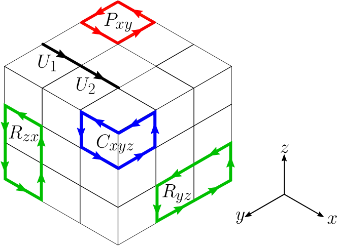
where and are the electric and magnetic field strengths with spatial components and . Alternatively, the magnetic energy density can be written in terms of , the spatial-spatial field strength tensor, as: with Latin indices indicating spatial directions as shown in Fig. 1. In terms of color components, , , with being generators of the gauge group. To ensure gauge invariance, lattice Hamiltonians are built from gauge links connecting lattice site to its neighbor in the spatial direction, with being the gauge coupling and the lattice gauge field [62]. By replacing the magnetic field term with the plaquettes (see Fig. 1 for and ) built from , and the electric field with the lattice electric field , one arrives at [58]:
| (2) | ||||
As temporal and spatial directions are treated differently, coupling and are introduced for the kinetic term and potential term , respectively. The discrepancy between and is of , as seen by series-expanding with denoting the covariant derivative:
| (3) |
For Symanzik improvement, one adds terms to , and adjusts couplings to cancel the discretization errors [63, 64]. The above classical error from can be cancelled by including the rectangle term (see Fig. 1), as detailed in the Supplementary Material. At the quantum level errors arise, requiring more terms, say the six-link bent loop terms (see Fig. 1).
The improved Hamiltonian can be written as with the improved potential term and the improved kinetic term [64]. is defined as
| (4) |
and has analogous expressions to . To cancel the errors in , one adds the two-link term :
| (5) |
For classical improvement, the couplings should be [63, 64]: , , , and . Perturbative improvements at the quantum level generate corrections of [61, 65]. One can further nonperturbatively tune these couplings numerically. For quantum simulations, these couplings could be extracted via analytic continuation of Euclidean calculations [55]. The resulting then has leading errors of to .
Both and can be derived from Euclidean actions via the transfer matrix in the continuous-time limit. The Lüscher-Weisz action [60] was used to derive [63, 64] and has improved errors of compared to the Wilson action used to derive [66]. For the Lüscher-Weisz action, fm lattices were found to have similar discretization errors to fm lattices with the Wilson action [67]. Similar scaling is suggested by the limited direct studies of and [68]. As the number of qubits required is , using may require fewer qubits in realistic quantum simulations for a fixed discretization error compared to . While we occupy ourselves with pure gauge theory, future effort should consider the fermion Hamiltonians [69] – particularly for chiral fermions.
Circuit Design - For quantum field theory calculations, is quantized by promoting the fields to operators: , . The magnetic field basis is the eigenbasis of the link operator while its Fourier transformation gives the electric field basis diagonalizing . The quantum state of a link is stored in a set of qubits - a link register. Any gauge circuit can be built from a set of primitive gates [70] acting on link registers:
-
•
inverse gate: ,
-
•
left and right multiplication gates: , ,
-
•
trace gate: ,
-
•
Fourier gate: with denoting the Fourier transform of .
-
•
L-phase gate: is a gauge group specific phase rotation, implemented by a diagonal matrix.
We implement the quantum circuits for term by term. Optimal quantum circuits depend on the underlying architecture – in particular connectivity. We assume register connectivity between a pair of links sharing a common site (linear register connectivity).
includes for every individual plaquette and the rectangles for every neighboring two plaquettes. We denote the circuits for as (Fig. 2(a)) and for the rectangles (Fig. 2(b)), with the coupling and trotter step encoded in . The circuit of Fig. 2(b) with registers appropriately changed implements .


The circuits for can be implemented by the L-phase gate in the electric field basis [70], as shown in Fig. 2(c). To avoid dealing with and operators simultaneously, we rewrite as
| (6) |
using the right electric field operator [19]:
| (7) |
For simplicity, we denote the two succeeding links in one direction as and following Fig. 1, and thus becomes . For non-Abelian gauge theories, this sum of non-commuting terms ( with color index ) is difficult to implement. We bypass this obstacle by decomposing as
| (8) |
With , the first two terms can be absorbed into . Thus, for the only new term is . Defining the evolution operator , and using , the matrix elements of are found to be (see Supplementary Material):
| (9) |
The circuit in Fig. 2(d) implements Eq. (9) by first storing the conserved quantity in the second register via , then performing on with the sequence . Finally, we ensure the conserved product of imposed by using the information stored in the second register via .
While using should require times fewer qubits, it requires additional gates to implement evolutions with the improved terms. Since the dominant quantum errors today are from decoherence and the entangling gates with error rates of [71, 72, 73], this increased cost may diminish the gain from using . We list the gate costs in terms of primitive gates in Tab. 1 for one trotter step using either or . Depending on which primitive gates dominate the circuits, the gate cost for is 2 to 4 times that of per link register. For the group and [74], different primitive gates take approximately the same order of entangling native gates. Since should require fewer link registers, for the cases of we anticipate the same or fewer total primitive gate cost.
| Gate | Impl. | ||
| 2 | 2 | ||
| 1 | 1 | ||
| CNOT |
Demonstration -


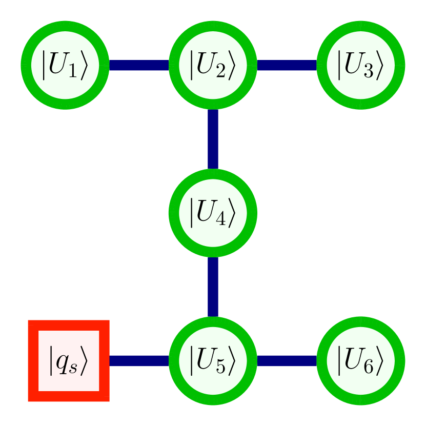
For gauge theory, can be mapped to Pauli matrices. Choosing the magnetic field basis, the qubit state () represents the element 1 (-1) of . Implementations of the primitive gates are listed in the last column of Tab. 1. We consider the most expensive gate, on the 7-qubit ibm_perth device (Fig. 3(c)). The connectivity of ibm_perth prevents implementing as shown in Fig. 3(a). With the mapping from links to qubits shown in Fig. 3(c), a transpiled version of the circuit with 12 CNOTs and 20 additional one-qubit gates are used. We use the benchmark value , precluding circuit optimization when using values such as .
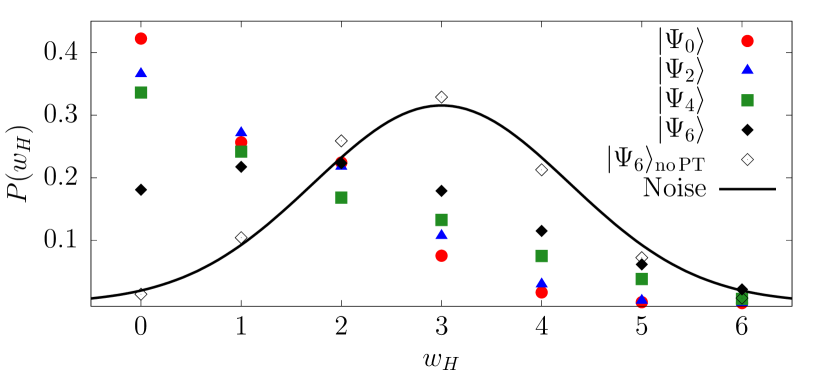
To quantify quantum errors, we evolve states with and its inverse, and compare the measurement with noiseless expectations, implemented as the circuit in Fig. 4. Without noise, the state preparation and are exactly cancelled by their complex conjugations, thus all measurements return , and the distribution of the Hamming weight – the number of qubits measured in the state – returns . In the noise-dominated limit where all states are equally populated, follows the binomial distribution with 6 trials.

We take as a definition of the quantum fidelity of for the state . Determining the fidelity requires testing all the possible states , a prohibitively expensive task [75]. Therefore we consider a restricted set consisting of for with indicating the qubit to which is applied.
To mitigate the coherent noise dominating the CNOT errors, we implement Pauli twirling [76, 77, 78, 79, 80] which converts coherent errors into random errors in Pauli channels and has found success in low-dimensional lattice field theories [81]. The circuits are modified by wrapping each CNOT with a set of Pauli gates randomly sampled from sets satisfying
| (10) |
where the -th qubit (including spectators) was rotated by before the CNOT and by after. Despite the enormous number of possible circuits, prior work has found circuits to be sufficient for error mitigation [76]. Therefore we implemented 15 unique circuits and run each circuit times. We also compute without Pauli twirling to gauge its effect.
With the above setup, we obtain the distribution in Fig. 5 for selected and the state-dependent fidelities (Table 2), yielding an average . Without Pauli twirling for , is indistinguishable from the noise-dominated limit while all the Pauli-twirled results are skewed toward the noiseless result, with states of lower (and consequently less average entanglement) being closer to the desired value. Comparing the results for with and without Pauli twirling we observe a fourfold improvement in fidelity – clearly demonstrating the advantage from this error mitigation.
| 0.650 | 0.575 | 0.605 | 0.599 | 0.579 | 0.442 | 0.425 | 0.1194 |
For a single trotter step, the time evolution of for a two-plaquette lattice with open boundary conditions requires at least 28 CNOTs (40 one-qubit gates): 12 CNOTs (20 one-qubit gates) for , at least 12 CNOTs (2 one-qubit gates) for the two and 4 CNOTs (6 one-qubit gates) for the two , alongwith 12 one-qubit gates for . Assuming that the average fidelity depends on the total number of CNOT gates, we can estimate the single-trotter-step fidelity for : . Thus current devices are inadequate for real-time computations. However given the expected hardware improvements in the coming years [36, 37, 38], will be improved, allowing simulations of a two-plaquette lattice for gauge theory and direct comparisons between Hamiltonians. Alternatively, classical simulators could explore lattices up to [82] to test improved Hamiltonians.
In this letter, we designed the quantum circuits for simulating the improved Hamiltonian . Comparing to the commonly used , should allow quantum simulations with fewer qubits. With this reduction, we expect the gate count to be comparable or less than that of for theories with despite increases of gate costs per link. For near-term numerical demonstrations, we constructed the circuits for of the gauge theory and found that for ibm_perth the fidelity of the 12 CNOT improved potential term is . Our results suggest that alongside hardware developments, improved Hamiltonians can accelerate quantum simulations by years by reducing the number of qubits required, with optimistic prospects for simulations in the near future.
Acknowledgements.
We would like to thank Erik Gustafson, Joseph Lykken and Michael Wagman for insightful discussions and comments on the manuscript. This work is supported by the Department of Energy through the Fermilab QuantiSED program in the area of “Intersections of QIS and Theoretical Particle Physics”. Fermilab is operated by Fermi Research Alliance, LLC under contract number DE-AC02-07CH11359 with the United States Department of Energy. We acknowledge use of the IBM Q for this work. The views expressed are those of the authors and do not reflect the official policy or position of IBM or the IBM Q team.References
- Yamamoto [2014] A. Yamamoto, Lattice QCD in curved spacetimes, Phys. Rev. D 90, 054510 (2014), arXiv:1405.6665 [hep-lat] .
- Lamm et al. [2020] H. Lamm, S. Lawrence, and Y. Yamauchi (NuQS), Parton physics on a quantum computer, Phys. Rev. Res. 2, 013272 (2020), arXiv:1908.10439 [hep-lat] .
- Kreshchuk et al. [2020] M. Kreshchuk, W. M. Kirby, G. Goldstein, H. Beauchemin, and P. J. Love, Quantum Simulation of Quantum Field Theory in the Light-Front Formulation (2020), arXiv:2002.04016 [quant-ph] .
- Echevarria et al. [2020] M. Echevarria, I. Egusquiza, E. Rico, and G. Schnell, Quantum Simulation of Light-Front Parton Correlators (2020), arXiv:2011.01275 [quant-ph] .
- Cohen et al. [2021] T. D. Cohen, H. Lamm, S. Lawrence, and Y. Yamauchi (NuQS), Quantum algorithms for transport coefficients in gauge theories, Phys. Rev. D 104, 094514 (2021), arXiv:2104.02024 [hep-lat] .
- Feynman [1982] R. P. Feynman, Simulating physics with computers, Int. J. Theor. Phys. 21, 467 (1982).
- Jordan et al. [2018] S. P. Jordan, H. Krovi, K. S. Lee, and J. Preskill, BQP-completeness of Scattering in Scalar Quantum Field Theory, Quantum 2, 44 (2018), arXiv:1703.00454 [quant-ph] .
- Bañuls et al. [2020] M. C. Bañuls et al., Simulating Lattice Gauge Theories within Quantum Technologies, Eur. Phys. J. D 74, 165 (2020), arXiv:1911.00003 [quant-ph] .
- Gustafson et al. [2020] E. Gustafson, H. Kawai, H. Lamm, I. Raychowdhury, H. Singh, J. Stryker, and J. Unmuth-Yockey, Exploring Digitizations of Quantum Fields for Quantum Devices, Snowmass 2021 LOI TF10-97 (2020).
- Hackett et al. [2019] D. C. Hackett, K. Howe, C. Hughes, W. Jay, E. T. Neil, and J. N. Simone, Digitizing Gauge Fields: Lattice Monte Carlo Results for Future Quantum Computers, Phys. Rev. A 99, 062341 (2019), arXiv:1811.03629 [quant-ph] .
- Alexandru et al. [2019] A. Alexandru, P. F. Bedaque, S. Harmalkar, H. Lamm, S. Lawrence, and N. C. Warrington (NuQS), Gluon field digitization for quantum computers, Phys.Rev.D 100, 114501 (2019), arXiv:1906.11213 [hep-lat] .
- Yamamoto [2021] A. Yamamoto, Real-time simulation of (2+1)-dimensional lattice gauge theory on qubits, PTEP 2021, 013B06 (2021), arXiv:2008.11395 [hep-lat] .
- Ji et al. [2020] Y. Ji, H. Lamm, and S. Zhu (NuQS), Gluon Field Digitization via Group Space Decimation for Quantum Computers, Phys. Rev. D 102, 114513 (2020), arXiv:2005.14221 [hep-lat] .
- Haase et al. [2021] J. F. Haase, L. Dellantonio, A. Celi, D. Paulson, A. Kan, K. Jansen, and C. A. Muschik, A resource efficient approach for quantum and classical simulations of gauge theories in particle physics, Quantum 5, 393 (2021), arXiv:2006.14160 [quant-ph] .
- Zohar et al. [2012] E. Zohar, J. I. Cirac, and B. Reznik, Simulating Compact Quantum Electrodynamics with ultracold atoms: Probing confinement and nonperturbative effects, Phys. Rev. Lett. 109, 125302 (2012), arXiv:1204.6574 [quant-ph] .
- Zohar et al. [2013a] E. Zohar, J. I. Cirac, and B. Reznik, Cold-Atom Quantum Simulator for SU(2) Yang-Mills Lattice Gauge Theory, Phys. Rev. Lett. 110, 125304 (2013a), arXiv:1211.2241 [quant-ph] .
- Zohar et al. [2013b] E. Zohar, J. I. Cirac, and B. Reznik, Quantum simulations of gauge theories with ultracold atoms: local gauge invariance from angular momentum conservation, Phys. Rev. A88, 023617 (2013b), arXiv:1303.5040 [quant-ph] .
- Zohar and Burrello [2015] E. Zohar and M. Burrello, Formulation of lattice gauge theories for quantum simulations, Phys. Rev. D91, 054506 (2015), arXiv:1409.3085 [quant-ph] .
- Zohar et al. [2016] E. Zohar, J. I. Cirac, and B. Reznik, Quantum Simulations of Lattice Gauge Theories using Ultracold Atoms in Optical Lattices, Rept. Prog. Phys. 79, 014401 (2016), arXiv:1503.02312 [quant-ph] .
- Zohar et al. [2017] E. Zohar, A. Farace, B. Reznik, and J. I. Cirac, Digital lattice gauge theories, Phys. Rev. A95, 023604 (2017), arXiv:1607.08121 [quant-ph] .
- Klco et al. [2020] N. Klco, J. R. Stryker, and M. J. Savage, SU(2) non-Abelian gauge field theory in one dimension on digital quantum computers, Phys. Rev. D 101, 074512 (2020), arXiv:1908.06935 [quant-ph] .
- Ciavarella et al. [2021] A. Ciavarella, N. Klco, and M. J. Savage, A Trailhead for Quantum Simulation of SU(3) Yang-Mills Lattice Gauge Theory in the Local Multiplet Basis (2021), arXiv:2101.10227 [quant-ph] .
- Bender et al. [2018] J. Bender, E. Zohar, A. Farace, and J. I. Cirac, Digital quantum simulation of lattice gauge theories in three spatial dimensions, New J. Phys. 20, 093001 (2018), arXiv:1804.02082 [quant-ph] .
- Wiese [2014] U.-J. Wiese, Towards Quantum Simulating QCD, Proceedings, 24th International Conference on Ultra-Relativistic Nucleus-Nucleus Collisions (Quark Matter 2014): Darmstadt, Germany, May 19-24, 2014, Nucl. Phys. A931, 246 (2014), arXiv:1409.7414 [hep-th] .
- Luo et al. [2019] D. Luo, J. Shen, M. Highman, B. K. Clark, B. DeMarco, A. X. El-Khadra, and B. Gadway, A Framework for Simulating Gauge Theories with Dipolar Spin Systems (2019), arXiv:1912.11488 [quant-ph] .
- Brower et al. [2019] R. C. Brower, D. Berenstein, and H. Kawai, Lattice Gauge Theory for a Quantum Computer, PoS LATTICE2019, 112 (2019), arXiv:2002.10028 [hep-lat] .
- Mathis et al. [2020] S. V. Mathis, G. Mazzola, and I. Tavernelli, Toward scalable simulations of Lattice Gauge Theories on quantum computers, Phys. Rev. D 102, 094501 (2020), arXiv:2005.10271 [quant-ph] .
- Singh [2019] H. Singh, Qubit nonlinear sigma models (2019), arXiv:1911.12353 [hep-lat] .
- Singh and Chandrasekharan [2019] H. Singh and S. Chandrasekharan, Qubit regularization of the sigma model, Phys. Rev. D 100, 054505 (2019), arXiv:1905.13204 [hep-lat] .
- Buser et al. [2020] A. J. Buser, T. Bhattacharya, L. Cincio, and R. Gupta, Quantum simulation of the qubit-regularized O(3)-sigma model (2020), arXiv:2006.15746 [quant-ph] .
- Raychowdhury and Stryker [2018] I. Raychowdhury and J. R. Stryker, Solving Gauss’s Law on Digital Quantum Computers with Loop-String-Hadron Digitization (2018), arXiv:1812.07554 [hep-lat] .
- Raychowdhury and Stryker [2020] I. Raychowdhury and J. R. Stryker, Loop, String, and Hadron Dynamics in SU(2) Hamiltonian Lattice Gauge Theories, Phys. Rev. D 101, 114502 (2020), arXiv:1912.06133 [hep-lat] .
- Davoudi et al. [2020] Z. Davoudi, I. Raychowdhury, and A. Shaw, Search for Efficient Formulations for Hamiltonian Simulation of non-Abelian Lattice Gauge Theories (2020), arXiv:2009.11802 [hep-lat] .
- Kan and Nam [2021] A. Kan and Y. Nam, Lattice Quantum Chromodynamics and Electrodynamics on a Universal Quantum Computer (2021), arXiv:2107.12769 [quant-ph] .
- Alexandru et al. [2021] A. Alexandru, P. F. Bedaque, R. Brett, and H. Lamm, The spectrum of qubitized QCD: glueballs in a gauge theory (2021), arXiv:2112.08482 [hep-lat] .
- ion [2020] Scaling IonQ’s quantum computers: The roadmap (2020).
- ibm [2021] IBM’s roadmap for building an open quantum software ecosystem (2021).
- Neven [2020] H. Neven, Day 1 opening keynote by Hartmut Neven (quantum summer symposium 2020) (2020).
- Trotter [1959] H. F. Trotter, On the product of semi-groups of operators, Proceedings of the American Mathematical Society 10, 545 (1959).
- Suzuki [1985] M. Suzuki, Decomposition formulas of exponential operators and lie exponentials with some applications to quantum mechanics and statistical physics, Journal of Mathematical Physics 26, 10.1063/1.526596 (1985), https://doi.org/10.1063/1.526596 .
- Şahinoğlu and Somma [2020] B. Şahinoğlu and R. D. Somma, Hamiltonian simulation in the low energy subspace (2020), arXiv:2006.02660 [quant-ph] .
- Hatomura [2022] T. Hatomura, State-dependent error bound for digital quantum simulation of driven systems (2022), arXiv:2201.04835 [quant-ph] .
- Campbell [2019] E. Campbell, Random compiler for fast Hamiltonian simulation, Phys. Rev. Lett. 123, 070503 (2019).
- Cirstoiu et al. [2020] C. Cirstoiu, Z. Holmes, J. Iosue, L. Cincio, P. J. Coles, and A. Sornborger, Variational fast forwarding for quantum simulation beyond the coherence time, npj Quantum Information 6, 1 (2020).
- Gibbs et al. [2021] J. Gibbs, K. Gili, Z. Holmes, B. Commeau, A. Arrasmith, L. Cincio, P. J. Coles, and A. Sornborger, Long-time simulations with high fidelity on quantum hardware (2021), arXiv:2102.04313 [quant-ph] .
- Yao et al. [2020] Y.-X. Yao, N. Gomes, F. Zhang, T. Iadecola, C.-Z. Wang, K.-M. Ho, and P. P. Orth, Adaptive variational quantum dynamics simulations, arXiv preprint arXiv:2011.00622 (2020).
- Berry et al. [2015] D. W. Berry, A. M. Childs, R. Cleve, R. Kothari, and R. D. Somma, Simulating Hamiltonian dynamics with a truncated Taylor series, Phys. Rev. Lett. 114, 090502 (2015).
- Low and Chuang [2019] G. H. Low and I. L. Chuang, Hamiltonian Simulation by Qubitization, Quantum 3, 163 (2019).
- Lamm and Lawrence [2018] H. Lamm and S. Lawrence, Simulation of Nonequilibrium Dynamics on a Quantum Computer, Phys. Rev. Lett. 121, 170501 (2018), arXiv:1806.06649 [quant-ph] .
- Harmalkar et al. [2020] S. Harmalkar, H. Lamm, and S. Lawrence (NuQS), Quantum Simulation of Field Theories Without State Preparation (2020), arXiv:2001.11490 [hep-lat] .
- Gustafson and Lamm [2021] E. J. Gustafson and H. Lamm, Toward quantum simulations of gauge theory without state preparation, Phys. Rev. D 103, 054507 (2021), arXiv:2011.11677 [hep-lat] .
- Yang et al. [2021] Y. Yang, B.-N. Lu, and Y. Li, Accelerated Quantum Monte Carlo with Mitigated Error on Noisy Quantum Computer, PRX Quantum 2, 040361 (2021), arXiv:2106.09880 [quant-ph] .
- Osterwalder and Schrader [1973] K. Osterwalder and R. Schrader, Axioms for Euclidean Green’s Functions, Commun. Math. Phys. 31, 83 (1973).
- Osterwalder and Schrader [1975] K. Osterwalder and R. Schrader, Axioms for Euclidean Green’s Functions. 2., Commun. Math. Phys. 42, 281 (1975).
- Carena et al. [2021] M. Carena, H. Lamm, Y.-Y. Li, and W. Liu, Lattice Renormalization of Quantum Simulations (2021), arXiv:2107.01166 [hep-lat] .
- Rajput et al. [2021] A. Rajput, A. Roggero, and N. Wiebe, Quantum error correction with gauge symmetries (2021), arXiv:2112.05186 [quant-ph] .
- Klco and Savage [2021] N. Klco and M. J. Savage, Hierarchical qubit maps and hierarchically implemented quantum error correction, Physical Review A 104, 10.1103/physreva.104.062425 (2021).
- Kogut and Susskind [1975] J. Kogut and L. Susskind, Hamiltonian formulation of Wilson’s lattice gauge theories, Phys. Rev. D 11, 395 (1975).
- Symanzik [1983] K. Symanzik, Continuum Limit and Improved Action in Lattice Theories. 1. Principles and phi**4 Theory, Nucl. Phys. B 226, 187 (1983).
- Luscher and Weisz [1985a] M. Luscher and P. Weisz, On-Shell Improved Lattice Gauge Theories, Commun. Math. Phys. 97, 59 (1985a), [Erratum: Commun. Math. Phys.98,433(1985)].
- Luscher and Weisz [1985b] M. Luscher and P. Weisz, Computation of the Action for On-Shell Improved Lattice Gauge Theories at Weak Coupling, Phys. Lett. B 158, 250 (1985b).
- Wilson [1974] K. G. Wilson, Confinement of quarks, Phys. Rev. D 10, 2445 (1974).
- Luo et al. [1999] X.-Q. Luo, S.-H. Guo, H. Kroger, and D. Schutte, Improved lattice gauge field Hamiltonian, Phys. Rev. D 59, 034503 (1999), arXiv:hep-lat/9804029 .
- Carlsson and McKellar [2001] J. Carlsson and B. H. McKellar, Direct improvement of Hamiltonian lattice gauge theory, Phys. Rev. D 64, 094503 (2001), arXiv:hep-lat/0105018 .
- [65] G. P. Lepage, Redesigning lattice qcd, Lecture Notes in Physics , 1–48.
- Creutz [1977] M. Creutz, Gauge Fixing, the Transfer Matrix, and Confinement on a Lattice, Phys. Rev. D15, 1128 (1977).
- Alford et al. [1995] M. G. Alford, W. Dimm, G. P. Lepage, G. Hockney, and P. B. Mackenzie, Lattice QCD on small computers, Phys. Lett. B 361, 87 (1995), arXiv:hep-lat/9507010 .
- Carlsson [2003] J. Carlsson, Improvement and analytic techniques in Hamiltonian lattice gauge theory, Other thesis (2003), arXiv:hep-lat/0309138 .
- Spitz and Berges [2019] D. Spitz and J. Berges, Schwinger pair production and string breaking in non-Abelian gauge theory from real-time lattice improved Hamiltonians, Phys. Rev. D 99, 036020 (2019), arXiv:1812.05835 [hep-ph] .
- Lamm et al. [2019] H. Lamm, S. Lawrence, and Y. Yamauchi (NuQS), General Methods for Digital Quantum Simulation of Gauge Theories, Phys. Rev. D100, 034518 (2019), arXiv:1903.08807 [hep-lat] .
- Wei et al. [2021] K. Wei, E. Magesan, I. Lauer, S. Srinivasan, D. Bogorin, S. Carnevale, G. Keefe, Y. Kim, D. Klaus, W. Landers, et al., Quantum crosstalk cancellation for fast entangling gates and improved multi-qubit performance (2021), arXiv:2106.00675 [quant-ph] .
- Lao et al. [2021] L. Lao, A. Korotkov, Z. Jiang, W. Mruczkiewicz, T. E. O’Brien, and D. E. Browne, Software mitigation of coherent two-qubit gate errors (2021), arXiv:2111.04669 [quant-ph] .
- Howe et al. [2021] L. Howe, M. Castellanos-Beltran, A. J. Sirois, D. Olaya, J. Biesecker, P. D. Dresselhaus, S. P. Benz, and P. F. Hopkins, Digital control of a superconducting qubit using a Josephson pulse generator at 3 K (2021), arXiv:2111.12778 [quant-ph] .
- Alam et al. [2021] M. S. Alam, S. Hadfield, H. Lamm, and A. C. Y. Li, Quantum Simulation of Dihedral Gauge Theories (2021), arXiv:2108.13305 [quant-ph] .
- Chuang and Nielsen [1997] I. L. Chuang and M. A. Nielsen, Prescription for experimental determination of the dynamics of a quantum black box, J. Mod. Opt. 44, 2455 (1997), arXiv:quant-ph/9610001 .
- Erhard et al. [2019] A. Erhard, J. J. Wallman, L. Postler, M. Meth, R. Stricker, E. A. Martinez, P. Schindler, T. Monz, J. Emerson, and R. Blatt, Characterizing large-scale quantum computers via cycle benchmarking, Nature Communications 10, 10.1038/s41467-019-13068-7 (2019).
- Li and Benjamin [2017] Y. Li and S. C. Benjamin, Efficient variational quantum simulator incorporating active error minimization, Physical Review X 7, 021050 (2017).
- Endo et al. [2018] S. Endo, S. C. Benjamin, and Y. Li, Practical quantum error mitigation for near-future applications, Physical Review X 8, 10.1103/physrevx.8.031027 (2018).
- Geller and Zhou [2013] M. R. Geller and Z. Zhou, Efficient error models for fault-tolerant architectures and the pauli twirling approximation, Physical Review A 88, 10.1103/physreva.88.012314 (2013).
- Wallman and Emerson [2016] J. J. Wallman and J. Emerson, Noise tailoring for scalable quantum computation via randomized compiling, Physical Review A 94, 10.1103/physreva.94.052325 (2016).
- Yeter-Aydeniz et al. [2022] K. Yeter-Aydeniz, Z. Parks, A. Nair, E. Gustafson, A. F. Kemper, R. C. Pooser, Y. Meurice, and P. Dreher, Measuring NISQ Gate-Based Qubit Stability Using a 1+1 Field Theory and Cycle Benchmarking (2022), arXiv:2201.02899 [quant-ph] .
- Gustafson et al. [2021] E. Gustafson et al., Large scale multi-node simulations of gauge theory quantum circuits using Google Cloud Platform, in IEEE/ACM Second International Workshop on Quantum Computing Software (2021) arXiv:2110.07482 [quant-ph] .