Distributed Optimal Power Flow for VSC-MTDC Meshed AC/DC Grids Using ALADIN

Abstract

The increasing application of voltage source converter (VSC)based high voltage direct current (VSC-HVDC)technology in power grids has raised the importance of incorporating DC grids and converters into the existing transmission network. This poses significant challenges in dealing with the resulting optimal power flow (OPF)problem. In this paper, a recently proposed nonconvex distributed optimization algorithm—Augmented Lagrangian based Alternating Direction Inexact Newton method (aladin), is tailored to solve the nonconvex AC/DC OPF problem for emerging voltage source converter (VSC)based multiterminal high voltage direct current (VSC-MTDC)meshed AC/DC hybrid systems. The proposed scheme decomposes this AC/DC hybrid OPF problem and handles it in a fully distributed way. Compared to the existing state-of-art Alternating Direction Method of Multipliers (admm), which is in general, not applicable for nonconvex problems, aladin has a theoretical convergence guarantee. Applying these two approaches to VSC-MTDC coupled with an IEEE benchmark AC power system illustrates that the tailored aladin outperforms admm in convergence speed and numerical robustness.

I Introduction

Due to AC grid expansion being limited by legislation and the capacity of long-distance transmission, high voltage direct current (HVDC)—especially voltage source converter (VSC)based multiterminal high voltage direct current (VSC-MTDC)technology—is being considered as an alternative solution. HVDC applications have traditionally been restricted to the transmission of power between two buses in the AC grids, which are almost exclusively built using thyristor based LCC-HVDC s. The main drawback of LCC-HVDC is that it cannot independently control the active and reactive power and suffers from commutation failure under inverter AC faults. Therefore it cannot be connected to very weak AC systems. On the contrary, VSC s can connect to very weak AC systems, they are able to independently control active and reactive power. This is benefical for controlling the voltage and frequency when connecting to renewable dominated grid. Another great advantage of VSC over LCC is that it can be employed in systems with more than two terminals, thereby forming a multi-terminal DC system. The world’s first commercial operational MTDC system, Italy-Corsica-Sardinia, was built in 1988 [1]. Now there are 35 VSC-HVDC systems in operation and 51 projects planned until 2019 [2, 3]. In Europe, a pan-European supergrid project is proposed for off-shore wind power transmission utilizing VSC-HVDC [4]. In China, commissioned VSC-MTDC projects, such as Nanao VSC-MTDC project [5], Zhoushan VSC-MTDC project [6], and Zhangbei VSC-MTDC project [7] are built. These projects suggest that the VSC-MTDC system has become a realistic solution for domestic and international power transmission.

Such VSC-MTDC system provides several advantages, including increased reliability of power transmission (by providing alternative paths), improved balancing services through AC interconnections (by controlling power flow), and reduced generation variability (by sharing the diverse portfolio of intermittent energy resources) [8, 9, 10]. Given that MTDC grids offer unique capability in terms of regulating power flow, which means that the VSC-MTDC meshed AC/DC system can be operated more flexibly and cost-effectively compared with point-to-point HVDC connections. As a result, the optimal power flow (OPF)problem of meshed AC/DC systems is becoming an urgent task to be investigated carefully. For the purpose of economic efficiency, OPF is used to determine the operating points of the meshed AC/DC grid. In [11], the first OPF algorithm was introduced for AC grids incorporating point-to-point HVDC connections, which is formulated as a quadratic programming problem without consideration for converter losses, converter transformers, and filters. In [12] and [13], a nonlinear AC/DC OPF model was proposed including a quadratic loss model for HVDC converters. In fact, the converter losses can add up to a significant fraction of the overall system losses. Thus, the converter losses should be carefully considered in the AC/DC OPF problem. In various literature [14, 15, 16, 17, 18], the converter losses are more accurately approximated by a quadratic function of its current magnitude. The AC/DC OPF problem is a nonconvex problem due to the nonlinear power flow equations and the highly nonlinear operating constraints imposed by the converters. Several methods have been proposed to address the AC/DC OPF with VSC-HVDC connections such as heuristic and interior point methods [14], Newton-Raphson method [19], second-order cone programming [20], sequential quadratic programming methods [21], or semidefinite programming relaxation methods [22]. Although the above literature has investigated the OPF of AC/DC systems, they are formulated in a centralized manner without fully considering the multilevel structure of VSC-MTDC meshed AC/DC systems.

Although regional grids are physically connected in this context, they make their generating plans independently, with very limited interactions with their neighbours. If a centralized optimization approach is adopted, all the generation information and network topology data needs to be acquired by a single central entity. This centralization may create substantial regulatory and political issues because the local system operators have to give up their governance and control to the central entity, which becomes almost impossible under the deregulated electricity market [8]. Hence, distributed optimization approaches have drawn significant attention in recent times. The most well-known distributed algorithms for tackling the AC OPF problems are Optimality Condition Decomposition (ocd) [23], Auxiliary Problem Principle (app) [24], and Alternating Direction Method of Multipliers (admm) [25, 26, 27]. ocd applies a modified Lagrangian relaxation decomposition. The original problem is partitioned into several subproblems, in which the local variables are decision variables and all foreign variables are fixed to the values of the previous iteration. By penalizing coupling constraints, ocd can converge to a solution with moderate accuracy under certain assumptions, e.g., relative weakly coupled subproblems, which cannot be guaranteed in general. In contrast to ocd, each subproblem shares the coupling variables with their neighbors and reformulates their objective function by using Augmented Lagrangian Relaxation in the context of both app and admm. Compared to app, admm reduces necessary information exchange and only requires neighbor-to-neighbor communication such that admm surpasses app in terms of communication effort. In [27, 28, 29], admm has been adopted to deal with the AC OPF problem. However, there are no generic convergence guarantees for AC OPF using the standard admm. Although [28] shows the convergence under some technical assumptions, the branch flow limits were not considered and these additional nonlinearities always result in divergence of admm. Recently,  [30] proposed a two-level admm approach, which as an exception, can deal with AC OPF problem with branch flow limits while guaranteeing convergence. Nevertheless, the AC OPF was formulated as a Quadratically Constrained Quadratic Program (qcqp)problem at the cost of accuracy, and it numerically converges slowly to a modest accuracy.

Different from these existing approaches, the Augmented Lagrangian based Alternating Direction Inexact Newton method (aladin)presented recently in [31] for distributed nonconvex optimization can provide a local convergence guarantee. As a distributed approach, the local agents’ associated subproblems are solved in the parallelizable step of aladin while an equality constrained quadratic program (qp)is solved in the consensus step, which is in principle close to a Sequential Quadratic Programming (sqp)step such that the convergence is sped up. At the expense of communication effort, aladin obtains locally quadratic convergence for nonconvex problems if suitable Hessian approximations are used, and a global convergence guarantee can also be achieved if the globalization strategy proposed in [31, Algorithm 3] is implemented.

Based on the existing literatures, there are still research gaps that need to be studied.

1. The traditional highly nonlinear and nonconvex OPF problem for meshed AC/DC hybrid systems is usually solved in a centralized manner. In reality, the different regional AC grids and the MTDC grid are owned and operated by different utilities under the deregulated electricity market, which is an independent decision-making process. Thus, the distributed optimization is much more preferable. Regarding the special structure of VSC-MTDC meshed AC/DC hybrid systems, it can be partitioned according to the grid-type naturally, and the resulting separated AC/DC OPF problem can be solved by applying a distributed algorithm.

2. In a practical VSC-MTDC meshed AC/DC hybrid systems, considering the AC branch flow limits, the DC branch flow limits, and the dynamic VSC operating constraints for meshed AC/DC hybrid systems leads to additional highly nonlinear and nonconvex inequality constraints in the resulting optimization problem such that the existing state-of-art distributed algorithms, such as admm, cannot guarantee the convergence. Recently, an exceptional distributed nonconvex optimization algorithm aladin has been investigated to deal with distributed AC OPF in [32] and distributed AC/DC hybrid OPF in [33] with convergence guarantee. The first is our previous work [32] that studied AC-OPF problem for the AC transmission system, which is the first journal paper applying aladin to deal with AC-OPF problem in a distributed manner. However, the most challenging AC branch flow limits were not considered. The second is literature [33] that adopted aladin to deal with the distributed AC/DC OPF problem for an oversimplified AC/DC hybrid system. However, the necessary and most challenging AC branch flow limits, DC branch flow limits, and highly nonlinear and nonconvex VSC operating constraints are all ignored. In terms of physical model, ignoring the AC and DC branch flow limits may lead to line overload; ignoring the essential dynamic operating constraints of VSC stations is unacceptable in the practical operation of VSC-MTDC meshed AC/DC grids (e.g. the converter power losses can add up to a significant fraction of the overall system losses, which are essential in the AC/DC OPF problem [16, 34, 22, 17]). In terms of mathematics, such an oversimplified scheme is much less practical and always leads to relatively weaker couplings between the AC grids and the DC grid. As a result, it is much easier to be solved by using distributed algorithms while heuristic implementation could simply work without encountering numerical challenges.

To fill these research gaps, this paper investigates the potential of using aladin for the highly nonlinear and nonconvex OPF problem of VSC-MTDC meshed AC/DC grids. The contributions are summarized as follows.

1. We consider complicated VSC-MTDC meshed AC/DC grids including AC/DC interconnections compared to the traditional point-to-point HVDC link. The full nonlinear and nonconvex AC/DC OPF model is built in an affinely coupled separable form and thus, is feasible for distributed algorithms. Compared to the existing oversimplified model on aladin-based distributed AC/DC OPF [33], this paper simultaneously takes the AC branch flow limits, the DC branch flow limits, and the complex dynamic operating model of VSC stations into account. Mathematically, this leads to additional highly nonlinear and nonconvex inequality constraints in the resulting optimization problem. Then, we tailor aladin algorithm to tackle this challenging nonconvex OPF problem in a distributed manner. At each iteration, the regional subproblems are solved in parallel while an equality constrained qp is solved in the consensus step, which is in principle close to a sqp step such that the convergence is sped up. The computation speed of the tailored aladin is numerically demonstrated to be faster than traditional centralized method. This indicates that the proposed approach will be of great potential in practical distributed implementation.

2. A detailed numerical investigation of aladin for the proposed AC/DC OPF problem is presented. Compared to the existing state-of-art admm, which is, in general, has no convergence guarantee for nonconvex problems, aladin has theoretical local convergence guarantee. In practice, although admm has been applied to solve nonconvex AC OPF [28, 29], one can always observe its divergence when including the branch flow limits. Our numerical comparison illustrates that aladin outperforms admm in all perspective for the proposed nonconvex AC/DC OPF problem. The improved performance comes at the cost of an increased per-step communication effort, which can be reduced by using quasi-Newton Hessian approximation. To this end, the number of iterations is slightly increased but aladin is still faster and more accurate than admm.

The rest of this paper is organized as follows: Section II presents the non-convex AC/DC OPF model. Section III introduces the distributed optimization formulation. Section IV presents numerical results. Section V concludes this paper.

II Problem Formulation

In this section, a mathematical model of the VSC-MTDC meshed AC/DC grids, e.g., the Zhangbei four terminal MTDC grid in China [7], is presented. Then, both centralized and distributed OPF formulations are respectively discussed.

II-A System Model of VSC-MTDC Meshed AC/DC Grids

Figure 1: VSC station schematic in VSC-MTDC meshed AC/DC grids with point of common coupling (PPC)

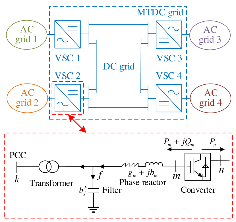
Fig. 1 shows the topology of the proposed grid model, which is abstracted from the Zhangbei four-terminal VSC-MTDC grid connected with four AC grids [7] in Northern China. The VSC station is considered with a transformer, AC filter, phase reactor, and converter. Without loss of generality, the VSC station is assumed to be a two- or three-level converter using the pulse-width modulation (PWM)switching method. We assume there is no generation or load in the MTDC grid.

Before discussing the grid model further, we introduce some nomenclature. We represent the meshed AC/DC grids by a tuple $(\mathcal{R},\mathcal{N},\mathcal{N}^{ac},\mathcal{N}^{mtdc},\mathcal{L},\mathcal{L}^{ac},\mathcal{L}^{mtdc})$. Thereby, $\mathcal{R}$ represents the set of all sub-grids, including 4 AC grids and a MTDC grid, i.e., $|\mathcal{R}|=5$, $\mathcal{N}=\mathcal{N}^{ac}\cup\mathcal{N}^{mtdc}$ denotes the set of all buses, $\mathcal{N}^{ac}$ the set of buses in AC grids, $\mathcal{N}^{mtdc}=\mathcal{N}^{vsc}\cup\mathcal{N}^{dc}$ the set of buses in MTDC grid, $\mathcal{N}^{dc}$ the set of buses in DC grid, $\mathcal{N}^{vsc}=\mathcal{N}_{ac}^{c}\cup\mathcal{N}_{dc}^{c}\cup\mathcal{N}_{ac}^{p}\cup\mathcal{N}_{ac}^{f}$ the set of all VSC buses, $\mathcal{N}_{ac}^{c}$ the set of AC side converter buses, $\mathcal{N}_{dc}^{c}$ the set of DC side converter buses, $\mathcal{N}_{ac}^{p}$ the set of PCC buses, $\mathcal{N}_{ac}^{f}$ the set of filter buses. $\mathcal{L}=\mathcal{L}^{ac}\cup\mathcal{L}^{mtdc}$ denotes the set of all branches, $\mathcal{L}^{ac}$ the set of branches in AC grids, $\mathcal{L}^{mtdc}$ the set of DC branches in MTDC grid. In Fig. 1, for example, bus $k$ is in set $\mathcal{N}_{ac}^{p}$, bus $f$ is in set $\mathcal{N}_{ac}^{f}$, bus $n$ is in set $\mathcal{N}_{dc}^{c}$, and bus $m$ is in set $\mathcal{N}_{ac}^{c}$.

II-B Objective

The objective of the AC/DC OPF problem is to jointly minimize the total generation cost and the total power losses on the branches and converters, where the total power losses are equal to the total generation minus the total load of the system. The objective of a subproblem can be divided into two parts, the total generation cost given by

$$C_{1}=\sum_{i\in\mathcal{N}^{ac}}\left\{c_{1i}\left(P_{i}^{G}\right)^{2}+c_{2i}P_{i}^{G}+c_{3i}\right\},$$ (1)

and the total system losses given by

$$C_{2}=\sum_{i\in\mathcal{N}^{ac}}\left(P_{i}^{G}-P_{i}^{D}\right),$$ (2)

where $c_{1i}$, $c_{2i}$, and $c_{3i}$ denote the cost coefficients of generator $i\in\mathcal{N}^{ac}$. $P_{i}^{G}$ and $P_{i}^{D}$ denote the generator active power output and load at bus $i$, respectively. If bus $i$ is not a generator bus, then, we have $P_{i}^{G}=0$ same to the load bus. For this, we only consider the active power losses of the system since the reactive power does not dissipate energy.

The objective function of the AC/DC OPF problem for VSC-MTDC meshed AC/DC grids is given by

$$C=C_{1}+\eta C_{2},$$ (3)

where $\eta$ denote a positive scaling coefficient. By increasing $\eta$, the total system losses have a larger weight in the objective function as compared with the generation cost. The typical value of $\eta$ is around the value of coefficients $c_{2i}$, since the total system losses is usually a linear function of the generators’ output. An appropriate value of $\eta$ can enable timely adjustment of control settings to jointly reduce the generation costs, VSC losses and transmission line losses. Thus, it can improve the operational economic efficiency of the entire system.

II-C Constraints of AC System

For the AC/DC OPF problem, the constraints of AC grids consist of power flow balance, branch flow limit and the limit on decision variables, i.e., voltage magnitude of all buses, as well as active and reactive power of generators.

II-C1 Nodal power balance of AC grid

$$P_{i}^{G}-P_{i}^{D}=V_{i}\sum_{j\in i}\left(G_{ij}\cos\theta_{ij}+B_{ij}\sin\theta_{ij}\right)V_{j},$$ (4a)

$$Q_{i}^{G}-Q_{i}^{D}=V_{i}\sum_{j\in i}\left(G_{ij}\sin\theta_{ij}-B_{ij}\cos\theta_{ij}\right)V_{j},$$ (4b)

with $i\in\mathcal{N}^{ac}$ and $j\in\mathcal{N}^{ac}\cup\mathcal{N}_{ac}^{p}$. Notice that the bus $l\in\mathcal{N}_{ac}^{p}$ belongs to VSC-MTDC system and branch $(l^{\prime},l)$ is the linking AC tie-line shown in Fig. 2. $G_{ij}$ and $B_{ij}$ denote the real and imaginary part in the admittance matrix. $Q_{i}^{G}$ and $Q_{i}^{D}$ denote the reactive power output of generator and reactive load at bus $i\in\mathcal{N}^{ac}$. $\theta_{ij}$ denotes the phase angle difference between buses $i$ and $j$. $V_{i}$ denotes the voltage magnitude of bus $i\in\mathcal{N}^{ac}$.

II-C2 Branch flow limit of AC grid

$$P_{ij} =V_{i}^{2}g_{ij}-V_{i}V_{j}\left(g_{ij}\cos\theta_{ij}+b_{ij}\sin\theta_{ij}\right)$$ (5a)

$$Q_{ij} =-V_{i}^{2}b_{ij}+V_{i}V_{j}\left(b_{ij}\cos\theta_{ij}-g_{ij}\sin\theta_{ij}\right)$$ (5b)

$$P_{ij}^{2} +Q_{ij}^{2}\leq\overline{S}_{ij}^{2}$$ (5c)

for all $\left(i,j\right)\in\mathcal{L}^{ac}$. Here $g_{ij}$ and $b_{ij}$ denote the conductance and susceptance of branch $\left(i,j\right)\in\mathcal{L}^{ac}$. $P_{ij}$ and $Q_{ij}$ denote the active and reactive power on branch $\left(i,j\right)\in\mathcal{L}^{ac}$. $\overline{S}_{ij}$ denotes the maximum allowable apparent power flow through branch $\left(i,j\right)\in\mathcal{L}^{ac}$.

II-C3 Limits on voltage magnitude, generator active and reactive power of AC grid

$$\underline{V}_{i} \leq V_{i}\leq\overline{V}_{i},\quad\;\,i\in\mathcal{N}^{ac},$$ (6a)

$$\underline{P}_{i}^{G} \leq P_{i}^{G}\leq\overline{P}_{i}^{G},\;\;i\in\mathcal{N}^{ac},$$ (6b)

$$\underline{Q}_{i}^{G} \leq Q_{i}^{G}\leq\overline{Q}_{i}^{G},\;\;i\in\mathcal{N}^{ac},$$ (6c)

where $\underline{V}_{i}$ and $\overline{V}_{i}$ denote the minimum and maximum nodal voltage magnitude at bus $i\in\mathcal{N}^{ac}$. $\underline{P}_{i}^{G}$ and $\overline{P}_{i}^{G}$ denote the minimum and maximum active power of generator $i\in\mathcal{N}^{ac}$. $\underline{Q}_{i}^{G}$ and $\overline{Q}_{i}^{G}$ denote the minimum and maximum reactive power of generator $i\in\mathcal{N}^{ac}$.

II-D Constraints of VSC-MTDC System

Constraints of the VSC-MTDC system consist of nodal power balance of MTDC system, operating limits of converters, as well as limits on branch flow and nodal voltage.

II-D1 Nodal power balance inside a VSC station

The power flow in a VSC station should satisfy the similar AC power balance at PCC bus $k$ and filter bus $f$, c.f. (4):

$$0= V_{i}\sum_{j\in i}\left(G_{ij}\cos\theta_{ij}+B_{ij}\sin\theta_{ij}\right)V_{j},$$ (7a)

$$-Q_{i}^{D}= V_{i}\sum_{j\in i}\left(G_{ij}\sin\theta_{ij}-B_{ij}\cos\theta_{ij}\right)V_{j}$$ (7b)

with $i\in\{k,f\}$ and $j\in\{k^{\prime},k,f,m\}$. Notice that the bus $k^{\prime}$ belongs to AC system and branch $(k^{\prime},k)$ is the linking AC tie-line shown in Fig. 2. The coupling between AC system and VSC-MTDC system will be discussed in the rest part of this section.

Regarding the reactive power of the AC filter, the demand at the AC filter bus, i.e., bus $f$, can be expressed as

$$Q_{f}^{D}=-V_{f}^{2}b_{f}^{F},\;f\in\mathcal{N}_{ac}^{f}$$ (8)

where $b_{f}^{F}$ denotes the shunt susceptance of the AC filter connected to bus $f$, while there is no reactive power demand at the PCC bus $k$.

II-D2 Voltage coupling between the converter AC bus and DC bus

The voltages of converter AC bus $m$ and DC bus $n$ are coupled by the PWM’s amplitude modulation factor, which can be set according to the modulation mode. The voltage magnitude at converter AC bus is upper bounded by [22, 35]

$$V_{m}\leq\delta V_{n},\;m\in\mathcal{N}_{ac}^{c},\;n\in\mathcal{N}_{dc}^{c},$$ (9)

where $V_{m}$ denotes the voltage magnitude at converter AC bus $m\in\mathcal{N}_{ac}^{c}$, $V_{n}$ the voltage at converter DC bus $n\in\mathcal{N}_{dc}^{c}$. $\delta$ denotes the PWM’s amplitude modulation factor.

II-D3 Active power coupling between the converter AC bus and DC bus

The coupling between the converter active power on AC side and DC side is described by

$$P_{m}+P_{n}+P^{loss}=0,\;m\in\mathcal{N}_{ac}^{c},\;n\in\mathcal{N}_{dc}^{c},$$ (10)

where $P_{m}$ and $P_{n}$ denote the active power at converter AC bus $m\in\mathcal{N}_{ac}^{c}$ and DC bus $n\in\mathcal{N}_{dc}^{c}$, respectively. $P^{loss}$ denotes the converter power losses.

The converter power losses can be approximated as a quadratic function of the phase current of the VSC valve as discussed in [22, 15],

$$P^{loss}=a_{1m}I_{m}^{2}+a_{2m}I_{m}+a_{3m},\;m\in\mathcal{N}_{ac}^{c}$$ (11)

with

$$I_{m}=\sqrt{\frac{P_{m}^{2}+Q_{m}^{2}}{V_{m}^{2}}},\;m\in\mathcal{N}_{ac}^{c},$$ (12)

where $I_{m}$ denotes the current magnitude at converter AC bus $m\in\mathcal{N}_{ac}^{c}$. $Q_{m}$ denotes the reactive power at converter AC bus $m\in\mathcal{N}_{ac}^{c}$. $a_{1m}$, $a_{2m}$, and $a_{3m}$ denote the conduction losses of the valves, the switching losses of valves and freewheeling diodes, and the no load losses of transformers and averaged auxiliary equipment losses, respectively. The values of the coefficients depend on the components and the power rating of the VSC station, and can be obtained using various approaches such as online identification or by aggregating the loss patterns of each component.

The converter losses contribute a relatively large percentage of the total system losses. The highly non-convex of converter losses adds a considerable computational burden for the AC/DC OPF problem in VSC-MTDC meshed AC/DC grids.

II-D4 Apparent capacity limit of a converter

The power injected into a converter from AC side is calculated by

$$P_{m}=V_{m}^{2}g_{m}-V_{m}V_{f}\left(g_{m}\cos\theta_{mf}+b_{m}\sin\theta_{mf}\right)$$ (13a)

$$Q_{m}=-V_{m}^{2}b_{m}+V_{m}V_{f}\left(b_{m}\cos\theta_{mf}-g_{m}\sin\theta_{mf}\right)$$ (13b)

for all $m\in\mathcal{N}_{ac}^{c}$ and $f\in\mathcal{N}_{ac}^{f}$. Here $g_{m}$ and $b_{m}$ denote the conductance and susceptance of phase reactor.

The VSC station is principally constrained by the maximum current through VSC valves and the maximum DC voltage [36]. The former determines the maximum VSC apparent power limit, and the latter defines the VSC reactive power output limit. In the present paper, VSC constraints at the converter AC bus are used because the VSC power exchange at the converter AC bus is set as control variables. The maximum current through the VSC valve has an upper limit as follows.

$$I_{m}\leq\overline{I}_{m},\;m\in\mathcal{N}_{ac}^{c},$$ (14)

where $\overline{I}_{m}$ denotes the maximum current through the VSC valve at converter AC bus $m\in\mathcal{N}_{ac}^{c}$.

Upon the substitution of (12) into (14), the apparent capacity limit of the converter is expressed as

$$P_{m}^{2}+Q_{m}^{2}\leq\left(V_{m}\overline{I}_{m}\right)^{2},\;m\in\mathcal{N}_{ac}^{c}.$$ (15)

II-D5 Reactive power limit of the converter

The operation of the VSC station is constrained by the upper and lower limits of the converter reactive power output. In practical VSCs, the maximum reactive power that the converter absorbs is approximately proportional to the nominal value of its apparent power [22, 16].

$$-\gamma S_{m}\leq Q_{m},\;m\in\mathcal{N}_{ac}^{c},$$ (16)

where $\gamma$ denotes a positive constant and can be determined by the type of the converter, $S_{m}$ denotes the nominal value of the apparent power of the converter.

According to [22, 15], since the susceptance $b_{m}$ of the phase reactor is normally much larger than its conductance $g_{m}$, the upper limit on the reactive power produced by the converter is expressed as

$$Q_{m}\leq-b_{m}\overline{V}_{m}\left(\overline{V}_{m}-V_{f}\right),\;m\in\mathcal{N}_{ac}^{c},f\in\mathcal{N}_{ac}^{f}.$$ (17)

where $\overline{V}_{m}$ denotes the maximum voltage magnitude of converter AC bus $m\in\mathcal{N}_{ac}^{c}$, $V_{f}$ the voltage magnitude of AC filter bus $f\in\mathcal{N}_{ac}^{f}$.

II-D6 Nodal power balance of DC grid

$$P_{n}=V_{i}\sum\limits_{\left({i,j}\right)\in{\mathcal{L}^{mtdc}}}{g_{ij}\left({V_{i}-V_{j}}\right)},\;i\in{\mathcal{N}^{dc}},n\in\mathcal{N}_{dc}^{c},$$ (18)

where $g_{ij}$ denotes the conductance of DC branch $(i,j)\in\mathcal{L}^{mtdc}$, $V_{i}$ denotes the nodal voltage of DC bus $i\in{\mathcal{N}^{dc}}$.

II-D7 Branch flow limit of DC grid

$$-\overline{P}_{ij}\leq{g_{ij}\left({V_{i}-V_{j}}\right)V_{i}}\leq\overline{P}_{ij},\;\left({i,j}\right)\in\mathcal{L}^{mtdc},$$ (19)

where $\overline{P}_{ij}$ denotes the maximum capacity of DC branch $(i,j)\in\mathcal{L}^{mtdc}$.

II-D8 Nodal voltage limit of DC grid

The terminal voltage of one DC bus in DC grid fixed as a reference has to satisfy the limit

$$\underline{V}_{i}\leq V_{i}\leq\overline{V}_{i},\;i\in{\mathcal{N}^{dc}}.$$ (20)

II-E Centralized and Distributed Problem

II-E1 Centralized Problem

The full AC/DC OPF Problem of VSC-MTDC meshed AC/DC grids is summarized as follows:

$$\text{minimize}\quad\eqref{eq::C}$$ (21)

subject to $$\eqref{eq::nodalAC}-\eqref{eq::Caceq},\eqref{eq::Smax}-\eqref{eq::voltDC}.$$

Overall, this full AC/DC OPF model is a non-convex nonlinear optimization problem, which could have solutions based on local optimums. The interior point method is commonly used in solving large-scale nonlinear optimization problems. This paper focuses on the formulation of the distributed non-convex optimization rather than on the development of the advanced solution algorithms for the global optimum of the nonlinear optimization problem. For different (local optimal) solutions with the same objective function value, the total costs obtained based on local optimums could be the same; however, the generation dispatches and system losses could be different.

For the proposed problem (21), it can only be directly solved in a centralized manner. However, the centralization will lead to the operation by a single central entity with complete knowledge and control of the entire meshed AC/DC grids. This centralization may create substantial regulatory and political issues because the local system operators have to give up their governance and control to the central entity. Thus, a distributed architecture is preferred. The distribution optimization repeatedly alternates solving a series small-scale subproblems and deploying a consensus step for coordination and hence, the iterative process is inevitable. However, this iterative process is worthwhile and essential as the distributed algorithm can not only preserve the information privacy and decision independence, but also comply with the philosophy of electricity market operations.

II-E2 Distributed Problem

Similar to [37], we reformulate the full AC/DC OPF problem in affinely coupled separable form amenable to distributed optimization. Operating the VSC-MTDC meshed AC/DC grids in a distributed way requires one to find the proper couplings between the regional AC grid and the MTDC grid. Take the coupling of AC grid 1 and MTDC grid as an example, shown in  Fig. 2(a),

Figure 2: Decomposition by sharing elements between neighboring regions

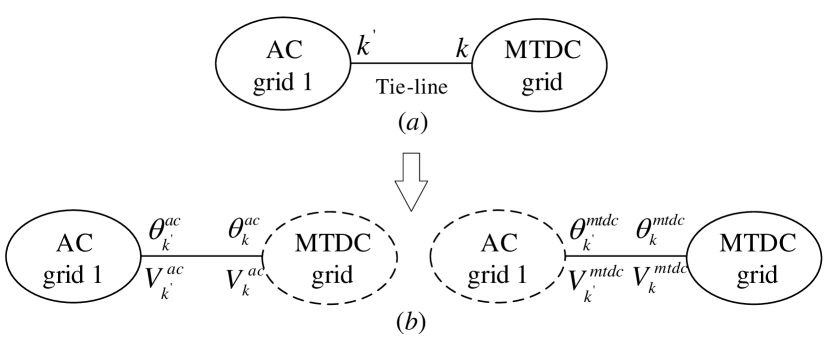
in which the system is divided into two parts that are connected through an AC tie-line between buses $k$ and $k^{\prime}$. Buses $k$ and $k^{\prime}$, and the linking AC tie-line are modeled together as a shared connection, labeled ($k$, $k^{\prime}$), between these two parts. This shared connection is taken into account in the local problems of the AC grid and the MTDC grid as shown in Fig. 2(b). In the proposed distributed optimization algorithm, the nodal voltage magnitude and the phase angle on buses $k$ and $k^{\prime}$ are coupled. Then, the consensus constraints are given by

$$V_{k}^{ac} =V_{k}^{mtdc},\;\;V_{k^{\prime}}^{ac}=V_{k^{\prime}}^{mtdcc},$$ (22a)

$$\theta_{k}^{ac} =\theta_{k}^{mtdc},\;\;\theta_{k^{\prime}}^{ac}=\theta_{k^{\prime}}^{mtc},$$ (22b)

which state that the complex voltage perceived by its connected zones should be identical.

Remark 1

The concept of sharing elements between neighboring regions allows one to compose the distributed OPF problem in a physically consistent manner: no additional modeling assumptions are introduced or required. If a solution to the distributed problem exists, then this will also be the solution to the respective centralized problem [27][37].

For each AC grid $\ell\in\mathcal{R}$, the local objective is given by

$$f_{\ell}(x_{\ell})=\sum_{i\in\mathcal{N}_{\ell}^{ac}} \left\{c_{1i}\left(P_{i}^{G}\right)^{2}+c_{2i}P_{i}^{G}+c_{3i}\right\}$$ (23)

$$\qquad\qquad\qquad+\eta\sum_{i\in\mathcal{N}_{\ell}^{ac}}\left(P_{i}^{G}-P_{i}^{D}\right),$$

with stacked local variables $x_{\ell}$, while the objective of the MTDC grid is set to be zero. This follows the fact that there is neither generator nor load in the MTDC grid. Hence, generation cost $C_{1}=0$ and losses term $C_{2}=0$ for the MTDC grid.

Based on the description in this section, the full hybrid OPF problem (21) can be summarized into the standard affinely coupled distributed form

$$\min_{x}\quad f(x):=\sum_{\ell\in\mathcal{R}}f_{\ell}(x_{\ell})$$ (24a)

s.t. $$\sum_{\ell\in\mathcal{R}}A_{\ell}x_{\ell}=0\quad\;\;\mid\lambda$$ (24b)

$$h_{\ell}(x_{\ell})\leq 0\qquad\quad\mid\kappa_{\ell},\;\ell\in\mathcal{R}$$ (24c)

$$\underline{x}_{\ell}\leq x_{\ell}\leq\overline{x}_{\ell}\qquad\mid\gamma_{\ell},\,\;\ell\in\mathcal{R}$$ (24d)

Here, the affine constraints (24b) summarize the coupling (22) between the AC grids and the MTDC grid. Constraints (24c) and (24d) collect all inequality constraints of each local model, where the box constraints (24d) denote the bounds on the local generator active/reactive power and nodal voltage magnitudes. In the following, we use notation

$$\tilde{h}(x_{\ell}):=[h_{\ell}(x_{\ell})^{\top}\;(x_{\ell}-\overline{x}_{\ell})^{\top}\;(\underline{x}_{\ell}-x_{\ell})^{\top}]^{\top}\leq 0,\;i\in\mathcal{R}$$

to stack (24c) and (24d). Moreover, we use notation $x$ to concatenate $x_{i}$ for all $i\in\mathcal{N}$, and throughout the rest of this paper, we write down the Lagrangian multipliers right after the constraints such that $\lambda$, $\kappa_{\ell}$, $\gamma_{\ell}$ denote the dual variables (multipliers) of constraints (24b), (24c), and (24d), respectively.

III Distributed Optimization Algorithm

This section presents admm and aladin as algorithms to approach a distributed solution. Both algorithms share the same idea—update primal variables in an alternating fashion, whereas the major difference lays in the consensus step.

III-A ADMM

The main idea of recalling admm is to use it as a benchmark method reflecting the current state-of-the-art. In order to apply admm for solving (21), we copy the variables $x_{\ell}$ and replace the consensus constraint (24b) by

$$x_{\ell}=z_{\ell}\quad\mid\xi_{\ell},\;\;\ell\in\mathcal{R}\quad\text{and}\quad 0=\sum_{i\in\mathcal{R}}A_{\ell}z_{\ell}$$ (25)

with Lagrangian multipliers $\xi_{\ell}$, $\ell\in\mathcal{R}$.

Algorithm 1 outlines the main steps of admm. Step 1 solves $|\mathcal{R}|$ decoupled problems that are constructed according to the augmented Lagrangian. Step 2 updates the dual iterate $\xi_{\ell}$ based on the gradient ascend method [38]. Notice that both Step 1 and 2 can be executed in parallel. Then, a practical terminal condition $\left\lVert\sum_{\ell\in\mathcal{R}}A_{\ell}x_{\ell}^{+}\right\rVert_{\infty}\leq\epsilon$ can be checked based on the local solution $x_{\ell}^{+}$. Step 3 deals a consensus QP whose solution can be worked out analytically, requiring one to collect $x_{\ell}^{+}$ and $\xi_{\ell}^{+}$. Once (27) is solved, the solution $z^{+}$ is broadcast to local agents, and the algorithm returns to Step 1.

Algorithm 1 admm

Input: $z$, $\xi$, $\rho>0$
Repeat:

1. update $x_{\ell}$ by solving all decoupled nlp problems

   $$x_{\ell}^{+}=\underset{\tilde{h}_{\ell}(x_{\ell})\leq 0}{\mathrm{argmin}}\quad f_{\ell}(x_{\ell})+\xi_{\ell}^{\top}x_{\ell}+\frac{\rho}{2}\left\lVert x_{\ell}-z_{\ell}\right\rVert^{2}_{2}$$ (26)

2. compute $\xi_{\ell}^{+}=\xi_{\ell}+\rho(x_{\ell}-z_{\ell})$, for all $\ell\in\mathcal{R}$.

3. update $z$ by solving the coupled averaging step

   hou

   $$z^{+}=\text{arg}\min_{z}\quad \sum_{\ell\in\mathcal{R}}\left\{\frac{\rho}{2}\left\lVert x_{\ell}^{+}-z_{\ell}\right\rVert_{2}^{2}-\xi_{\ell}^{\top}z_{\ell}\right\}\quad$$ (27a)

   s.t. $$\sum_{\ell\in\mathcal{R}}A_{\ell}z_{\ell}=0$$ (27b)

Remark 2

By taking advantage of the topological structure, solving (27) in the consensus step 3 of Algorithm 1 could only require neighbor-to-neighbor communications. This follows the fact that matrices $A_{\ell}$ denote the adjacency of the graph. More details refer to [39].

III-B ALADIN

aladin, originally proposed in [31], is developed for dealing with generic distributed nonlinear programming. Solving (24) by using aladin is outlined in Algorithm 2. Similar to admm, Steps 1 and 2 of Algorithm 2 are parallelizable. The local problems (28) are also formulated following the idea of the augmented Lagrangian. Here, one may adjust either the scaling matrices $\Sigma_{\ell}$ or penalty parameter $\rho$ during the iterations in order to improve performance. A practical strategy to update $\rho$ for distributed AC OPF can be found in [32]. Based on the local solutions $x_{\ell}$, the algorithm terminates if

$$\left\lVert\sum_{\ell\in\mathcal{R}}A_{\ell}x_{\ell}\right\rVert_{\infty}\leq\epsilon\;\text{and}\;\max_{\ell}\left\lVert\Sigma_{\ell}(x_{\ell}-z_{\ell})\right\rVert_{\infty}\leq\epsilon.$$

holds. This condition implies that $x_{\ell}$ satisfies the first order optimality condition of (24)

$$\left\|\nabla\left\{f_{\ell}(x_{\ell})+\kappa^{\top}h_{\ell}(x_{\ell})+\gamma_{\ell}^{\top}x_{\ell}\right\}+A_{\ell}^{\top}\lambda\right\|\leq\epsilon$$

up to the user-specified numerical tolerance $\epsilon$. As discussed in [31], the iterate $(x,\lambda,\kappa,\gamma)$ is a primal-dual KKT point of Problem (24)—up to the user specified numerical accuracy $\epsilon$. Step 2 evaluates the sensitivities at the local primal-dual solutions. Here, the Hessian approximation (30) is required to be positive definite such that QP (31) is convex and has unique solution. In practice, some numerical heuristics can be applied to make it be satisfied such as adding a small regularization. In our implementation, we adopt the heuristic implemented in open-source toolkit ACADO [40], which flips the negative eigenvalue of $H_{\ell}$.

Algorithm 2 aladin

Input: $z$, $\lambda$, $\rho>0$, $\mu>0$ and scaling symmetric matrices $\Sigma_{\ell}\succ 0$
Repeat:

1. solve the following decoupled nlp s for all $\ell\in\mathcal{R}$

   $$\min_{x_{\ell}}\quad f_{\ell}(x_{\ell})+\lambda^{\top}A_{\ell}x_{\ell}+\frac{\rho}{2}\left\lVert x_{\ell}-z_{\ell}\right\rVert^{2}_{\Sigma_{\ell}}$$ (28a)

   s.t. $$h_{\ell}(x_{\ell})\leq 0\qquad\mid\kappa_{\ell},$$ (28b)

   $$\underline{x}_{\ell}\leq x_{\ell}\leq\overline{x}_{\ell}\quad\mid\gamma_{\ell}$$ (28c)

2. compute the Jacobian matrix $J_{\ell}$ based on the active set at the local solution $x_{\ell}$ by

   $$[J_{\ell}]_{i}=\begin{cases}\partial\;[\tilde{h}_{\ell}(x_{\ell})]_{i}&\text{if }[\tilde{h}_{\ell}(x_{\ell})]_{i}=0\\[3.41418pt] 0&\text{otherwise}\end{cases}$$ (29)

   with $[J_{\ell}]_{i}$ the i-th row of matrix $J_{\ell}$ and gradient $g_{\ell}=\nabla f_{\ell}(x_{\ell})$, choose Hessian approximation

   $${\color[rgb]{0,0,0}H_{\ell}\approx\nabla^{2}\left\{f_{\ell}(x_{\ell})+\kappa_{\ell}^{\top}h_{\ell}(x_{\ell})\right\}\succ 0.}$$ (30)

3. solve coupled qp

$$\min_{\Delta x,s} \sum_{\ell\in\mathcal{R}}\left\{\frac{1}{2}\Delta x_{\ell}^{\top}\;H_{\ell}\;\Delta x_{\ell}+g_{\ell}^{\top}\Delta x_{\ell}\right\}+\lambda^{\top}\;s+\frac{\mu}{2}\left\lVert s\right\rVert^{2}_{2}$$ (31a)

s.t. $$\quad\sum_{\ell\in\mathcal{R}}A_{\ell}(x_{\ell}+\Delta x)=b+s\quad\mid\lambda^{QP}$$ (31b)

$$\quad J_{\ell}\Delta x_{\ell}=0,\;\;\ell\in\mathcal{R}\;.$$ (31c)

1. update primal and dual variable $z$, $\lambda$ by

   $$z^{+} =x+\alpha_{1}(x-z)+\alpha_{2}\Delta x,$$ (32a)

   $$\lambda^{+} =\lambda+\alpha_{3}(\lambda^{QP}-\lambda),$$ (32b)

   where the line search scheme [31, Algorithm 3] can be used to calculate the step sizes $\alpha_{1}$, $\alpha_{2}$ and $\alpha_{3}$.

Notice that the size of Jacobian matrices $J_{\ell}$ is changed during the iterations as the active set might be changed. In practice, if the quasi-Newton Hessian approximation such as Broyden–Fletcher–Goldfarb–Shanno (bfgs) is used to compute $H_{\ell}$, the communication cost can be significantly reduced [32]. The main difference between admm and aladin is the consensus step. While both approaches require one to solve a qp problem, different from (27), Problem (31) is equivalent to an inexact Newton step for solving (24) with only considering the active constraints at the local solution $x_{\ell}$. This is crucial for the convergence improvement of aladin. Notice that introducing the slack variables $s$ in (31) guarantees that Problem (31) is always feasible no matter if the original problem (24) is feasible or not. In practice, solving the equality constrained QP (31) only needs a basic linear algebraic routine such as Lapack as it is equivalent to solve the resulting KKT system based linear equations. Its analytical solution can be found in Appendix. One can see that if the full step is applied at Step 4, only the dual update (36) requires communication while it is not necessary to communicate all sensitivities. Thus, if there exists a central entity or any local agent could perform as a central coordinator, Step 3 can be efficiently implemented. Moreover, if only neighbor-to-neighbor communication is allowed, [41] has proposed bi-level distributed variants of aladin, in which three methods, including Schur complement method, decentralized ADMM method and decentralized conjugate gradient method, was adopted to deal with (31) in a decentralized manner.

The overall frameworks of Algorithms 1 and 2 are similar. However, in general, applying admm to nonconvex optimization (24) does not have any theoretical guarantees. In contrast to this, aladin has a local convergence guarantee while the globalization presented in [31, Algorithm 3] can guarantee the global convergence with doing line search in Step 4) of Algorithm 2. In this paper, we focus on the local convergence properties of Algorithm 2 as in practice, according to the physical model of the power grids, a good initial guess of the primal-dual iterates can be obtained. In order to introduce the local convergence results of Algorithm 2, we need the following definition.

Definition 1

A KKT point for generic constrained optimization is called regular [42] if the linear independence constraint qualification (LICQ), strict complementarity conditions (SCC), as well as the second order sufficient condition (SOSC) are satisfied.

Now, we summarize the local convergence property of Algorithm 2 as follows:

Theorem 1

Let the KKT point $(z^{*},\lambda^{*},\kappa^{*},\gamma^{*})$ of Problem (24) be regular such that following the SOSC it is a local minimizer. And let the penalty parameter $\rho<\infty$ in Algorithm 2 be sufficiently large with $\nabla^{2}\left\{f_{\ell}(x_{\ell})+\kappa_{\ell}^{\top}h_{\ell}(x_{\ell})\right\}+\rho\Sigma_{\ell}\succ 0$. Moreover, let matrices

$$H_{\ell}=\nabla^{2}\left\{f_{\ell}(x_{\ell})+\kappa_{\ell}^{\top}h_{\ell}(x_{\ell})\right\}+\mathcal{O}(\|x_{\ell}-z_{\ell}\|)$$ (33)

holds for all $\ell\in\mathcal{R}$, the iterates $x_{\ell}$ of Algorithm 2 converge locally with quadratic rate if full step size is appled in Step 4), i.e., $\alpha_{1}=\alpha_{2}=\alpha_{3}=1$.

Here, the local convergence means that the initial guess of primal-dual iterates are located in a small neighborhood at the local minimizer $(x^{*}=z^{*},\lambda^{*})$. The proof of Theorem 1 can be established in two steps. First, according to the assumptions of regularity and $\rho$, the local minimizer of subproblems (28), $x_{\ell}$ is parametric with $(z,\lambda)$ and the solution maps are Lipschitz continuous, i.e., there exists constants $\chi_{1},\chi_{2}>0$ such that

$$\left\|x-z^{*}\right\|\leq\chi_{1}\left\|z-z^{*}\right\|+\chi_{2}\left\|\lambda-\lambda^{*}\right\|.$$ (34)

This result was formally stated in [31, Lemma 3] and the proof can be established by applying the implicit function theorem [42, Appendix 2, Page 630], which refer to [43, Lemma 1] for more details. The second step follows the fact that the active sets are not changed locally based on the assumptions. Then, the standard analysis of Newton’s method [42, Chapter 3.3] gives

$$\left\|\begin{bmatrix}z^{+}-z^{*}\\ \lambda^{+}-\lambda^{*}\end{bmatrix}\right\|\leq \left\|H-\nabla^{2}f(x)+\kappa^{\top}h_{\ell}\right\|\cdot\mathcal{O}\left(\left\|x-z^{*}\right\|\right)$$

$$+\mathcal{O}\left(\left\|x-z^{*}\right\|^{2}\right)$$

Based on condition (33), we have that there exists a constant $\sigma>0$ such that the local quadratic contraction

$$\left\|z^{+}-z^{*}\right\|\leq\sigma\left\|x-z^{*}\right\|^{2}\;\;\text{and}\;\;\left\|\lambda^{+}-\lambda^{*}\right\|\leq\sigma\left\|x-z^{*}\right\|^{2}$$ (35)

can be established. Combing (34) and (35) yields the result. A more detailed proof of Theorem 1 can be found in [31, Section 7].

Remark 3

If we use BFGS Hessian approximation, a local superlinear convergence rate is achieved instead [44]. The analysis is close to Theorem 1 with slight difference in the second step of the proof.

Remark 4

In practice, only a numerical solution of decoupled problem (28) is achievable while convergence result in Theorem 1 can be still established by assuming that the local solutions of (28) is bounded by $\left\|\bar{x}-x\right\|\leq\zeta\left\|x-z\right\|$ with $\bar{x}$ the approximate solution given by the numerical solver. The proof refers to [32, Theorem 2]

IV Numerical Results

Figure 3: Convergence behavior of admm for Case 1

Figure 4: Convergence behavior of aladin for Case 1

Figure 5: Coupling variables convergence towards optimal value of aladin with exact Hessian for Case 1

Figure 6: Coupling variables convergence towards optimal value of aladin with inexact Hessian for Case 1

Figure 7: Convergence behavior of aladin using exact Hessians for Case 2

This section illustrates the performance of the proposed distributed algorithms with comparison to admm. The model is merged by a four-terminal VSC-HVDC network with four AC grids from Matpower [45], which are modified using open-source rapidpf toolbox, proposed in [37].

In Case 1 a VSC-HVDC network is connected with four IEEE 9-bus AC grids as shown in Fig. 1 while a VSC-HVDC network is connected with four IEEE 118-bus AC grids in Case 2. Bus 2 and Bus 8 are the connecting bus for 9-bus AC grid and 118-bus AC grid respectively. For both Cases, base power and base voltage is set to 100MVA and 345kV; voltage magnitude of both AC and DC grid are limited to [0.95, 1.05] p.u.; the master VSC station connecting to AC grid 3 keeps 1 p.u. to provide the constant DC voltage reference; the parameters for VSC stations and DC branches in the grid’s per-unit system (p.u.)are given in  Table I and II to differentiate the four AC grids in both Cases, the generator cost coefficients and load of AC regions 1 and 2 are set to be smaller than regions 3 and 4, shown in Table III. In this way, we force the power exports from AC regions 1 and 2 to regions 3 and 4. The scaling coefficient for system loss term is set to $\eta=10$ to jointly minimize the total generation cost and system losses. For reasons of a fair comparison, our implementation initializes the primal variables $x$ for each AC block with 1 p.u for voltage magnitudes while 0 for all other values. This flat starting strategy is standard, which was used in literature, for example, [32, 37], and also chosen as the default strategy in Matpower [45]. For the MTDC block, we applied a similar strategy that intuitively initialized voltage magnitudes by $1$ p.u, and the injected power by $0$. The initial dual variable $\lambda$ are set to zero (flat start).

Applying admm and aladin to solve problems requires selecting tuning parameters $\rho$ and $\mu$. To enable a fair comparison, these parameters are determined by parameter sweeps aiming for fast convergence, shown in Table IV. To obtain a similar scaling, the weighting matrices are chosen such that each diagonal entry is inversely proportional to its corresponding decision variable range, as suggested in [32].

TABLE I: VSC station parameters

Term	Value	Term	Value	Term	Value
$a_{1m}$	0.011 p.u.	$R_{m}$	0.00025 p.u.	$R_{f}$	0.0005 p.u.
$a_{2m}$	0.003 p.u.	$X_{m}$	0.04 p.u.	$X_{f}$	0.0125 p.u.
$a_{3m}$	0.0043 p.u.	$B_{f}$	0.2 p.u.	$S_{m}$	11 p.u.
$\delta$	1.05	$\gamma$	0.5	$\overline{V}_{m}$	1.05 p.u.
$\overline{I}_{m}$	11 p.u.

TABLE II: DC branch parameters

Line No.	From bus	To bus	Resistance [pu]	Flow limit [pu]
				Case 1	Case 2
1	1	2	0.00042	1.5	8
2	1	3	0.00174	1.5	8
3	2	4	0.00175	1.5	8
4	3	4	0.00159	1.5	8

TABLE III: Load and generator cost coefficients ratio setting

	AC grid No.	$P^{D}$ [MW]	$Q^{D}$ [MVar]	Cost Coefficients ratio
Case 1	1	315	115	1.0
	2	318	116	1.3
	3	321	117	1.7
	4	324	118	2.2
Case 2	1	4242	1438	1.0
	2	4666	1582	1.3
	3	5090	1726	1.7
	4	5515	1869	2.2

TABLE IV: Algorithm parameters of admm and aladin

Parameters	ADMM		ALADIN-BFGS		ALADIN
	Case 1	Case 2	Case 1	Case 2	Case 1	Case 2
$\rho$	$10^{4}$	-	$10^{4}$	-	$10^{2}$	$10^{2}$
$\mu$	-	-	$10^{3}$	-	$10^{3}$	$10^{3}$

The framework is built on Matlab-R2021a and the AC grid modeling follows AC-OPF model of Matpower. The case studies are carried out on a standard desktop computer with Intel^® i5-6600K CPU @ 3.50GHz and 16.0 GB installed ram. casadi toolbox [46] is used in Matlab and ipopt [47] is used as the solver for both the decoupled nlp s and the coupled qp. The computation time is posted in Table V.

TABLE V: Comparisons of different algorithms for Cases 1 and 2

Case	Algorithm	Iterations	Time [s]	$\left\lVert x-x^{*}\right\rVert_{\infty}$	Generation Cost $C_{1}$		System Losses $C_{2}$
					Cost [$\times 10^{2}\$$]	Solution gap	Losses [MW]	Solution gap
1	Centralized	-	$0.181$	-	$249.354$	-	$23.484$	-
	admm	$\geq 3\times 10^{4}$	$\geq 3000$	$0.151$	$249.141$	$8.56\times 10^{-4}$	$23.505$	$8.95\times 10^{-4}$
	aladin-bfgs	$49$	$0.700$	$5.62\times 10^{-3}$	$249.354$	$2.03\times 10^{-8}$	$23.484$	$1.77\times 10^{-6}$
	aladin	$9$	$0.142$	$7.52\times 10^{-6}$	$249.354$	$7.94\times 10^{-7}$	$23.484$	$1.978\times 10^{-7}$
2	Centralized	-	$1.465$	-	$9547.316$	-	$515.985$	-
	admm	Did not converge
	aladin-bfgs	Did not converge
	aladin	$13$	$0.878$	$1.50\times 10^{-6}$	$9547.316$	$6.63\times 10^{-9}$	$515.985$	$7.59\times 10^{-9}$

Similar to [32], we use the following quantities in order to depict the algorithm convergence behavior. The reference solution $x^{*}$ is obtained by solving problem (21) with ipopt centrally.

1. The deviation of optimization variables from the optimal value $\left\lVert x-x^{*}\right\rVert_{\infty}$.

2. The consensus violation $\left\lVert Ax\right\rVert_{\infty}=\left\lVert\sum_{\ell\in\mathcal{R}}A_{\ell}x_{\ell}\right\rVert_{\infty}$.

3. The dual residual $\left\lVert r\right\rVert_{\infty}$ with $r=\sum_{\ell\in\mathcal{R}}\left\{A_{\ell}(x_{\ell}-z_{\ell})\right\}$ for admm, $r=\sum_{\ell\in\mathcal{R}}\left\{\Sigma_{\ell}(x_{\ell}-z_{\ell})\right\}$ for aladin.

4. The solution gap between a specific distributed algorithm and the centralized algorithm is calculated as $\frac{f(x)-f(x^{*})}{f(x^{*})}$.

Remark 5

When the problem is feasible, it means that the VSC-MTDC Meshed AC/DC Grid has at least one safe operating point, in which neither the transmission lines nor the converters are overloaded, etc. Meanwhile, the correct solution represents the operating point with the best economic efficiency for the grid.

IV-A Four-Terminal VSC-HVDC with Four IEEE 9-bus AC Grids

IV-A1 ADMM vs. ALADIN

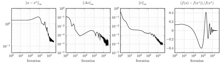
In general, admm has no convergence guarantee for and AC-OPF problem, especially when the AC branch flow limits are implemented as the nonlinear inequality constraint[32]. The mathematical model of VSC-MTDC meshed AC/DC grids is much more complicated and the convergence of admm is highly sensitive to the tuning parameters. Fig. 3 shows the convergence behaviors of admm, with tuning parameter $\rho=10^{4}$. It is observed that admm requires thousands of iterations to converge to modest accuracy, i.e., $\epsilon=10^{-4}$. To approach higher accuracy, primal variables $y$ start damping near the optimizer. Nevertheless, the solution gap by applying admm is acceptable for practical use.

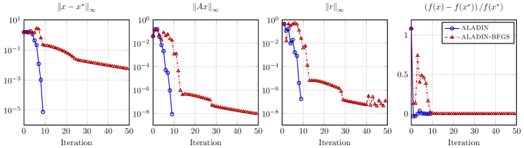
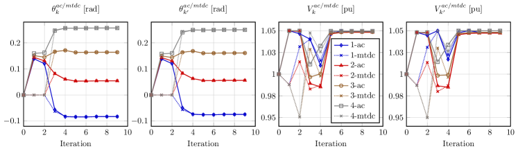
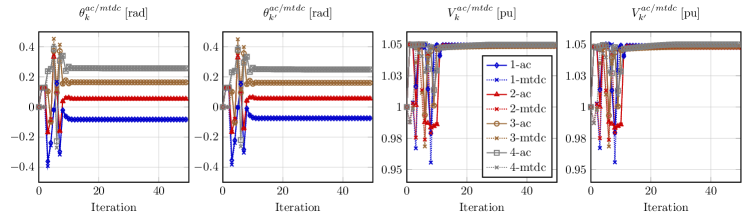
In contrast to admm, aladin obtains curvature information of all subproblems in the central coordinator and has the ability to deal with the non-convex constraints. Fig. 4 presents convergence behavior of aladin with two different methods for computing the Hessian matrix. It is obvious that aladin converges significantly faster than admm. Unlike admm, the solution gap of aladin is fairly small compared with the centralized method, as shown in Table V. The number of iterations and the computation time in aladin is much less than admm. The computational costs per iteration are only slightly higher for aladin, which leads to a strong computation time decrease while much higher accuracy in terms of the optimal gap and dual residual are obtained. In summary, despite higher communication effort, aladin surpasses admm in all perspective for solving the AC/DC OPF problem of VSC-MTDC meshed AC/DC grids.

IV-A2 Exact Hessian vs. BFGS

To reduce the per-step communication effort between decoupled nlp s and the central coordinator, the bfgs method is implemented to avoid communicating the full Hessian matrix. Considering the theoretically worst case, i.e., all matrices and vectors required to communicate are dense without zero elements, Algorithm 2 with exact Hessian requires to communicate

$$\sum_{\ell\in\mathcal{R}}\underbrace{n_{\ell}}_{g_{\ell}}+\underbrace{\frac{n_{\ell}(1+n_{\ell})}{2}}_{\text{symmetric}\;H_{i}}+\underbrace{n_{\ell}\sum_{j\in\mathcal{A}_{\ell}}m_{i}}_{J_{\ell}}$$

float numbers in forward communication while using BFGS update can reduce this number as $\sum_{\ell\in\mathcal{R}}\left(3n_{\ell}+n_{\ell}\sum_{i\in\mathcal{A}_{\ell}}m_{i}\right)$. Here, $n_{\ell}$ defines the dimension of $x_{\ell}$ and set $\mathcal{A}_{\ell}$ collects the index of the active inequality constraints $[\tilde{h}_{\ell}(x_{\ell})]_{i}=0$ at local solution $x_{\ell}$. Fig. 4 compares the convergence behaviors of using exact Hessian and using bfgs to approximate Hessian for solving the AC/DC OPF problem. For both options, aladin can converge to a solution with modest accuracy, i.e., $\epsilon=10^{-4}$ for all termination criteria, within a dozen iterations. Furthermore, aladin using inexact Hessians needs just slightly more iterations compared with aladin using exact Hessians. One can observe that the convergence rate for aladin using inexact Hessians is faster than linear. Nonetheless, it needs several dozens more iterations to converge when a high accurate solution is required, while aladin with exact Hessian needs only several iterations.

In the perspective of coupling variables, as illustrated in Fig. 5 and 6, the nodal voltage magnitude and phase angle of boundary bus and fictitious bus among the local AC grids and MTDC grid converge to the same operating point after $9$ iterations (exact Hessians) and $49$ iterations (inexact Hessians), respectively.

IV-B Four-Terminal VSC-HVDC with Four IEEE 118-bus AC Grids

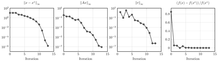
The performance of the proposed algorithm is further analyzed on a larger VSC-MTDC meshed AC/DC grid in Case 2. As summarized in Table V, the admm and aladin-bfgs fail to converge for solving this larger system no matter how the step size $\rho$ is adapted. The algorithm convergence behavior for Case 2 using aladin with exact Hessians is depicted in Fig. 7. Similar to Case 1, the solution gap of aladin is fairly small compared with the centralized method.

The proposed aladin algorithm with exact Hessian takes 0.142 and 0.878 seconds for the two cases, respectively, and the computation time of aladin is slightly faster than the centralized approach that takes 0.181 and 1.465 seconds, respectively. In conclusion, aladin with exact Hessian outperform both centralized approach and admm method for the two cases. This indicates that aladin has more potential in practical distributed implementation.

V Conclusions

To fully coordinate the AC grids and the MTDC grid to mutually benefit multiple regions, the present paper tailors the recently proposed novel distributed aladin algorithm to solve the non-convex AC/DC OPF problem for the VSC-MTDC meshed AC/DC grids. By operating the AC grids and MTDC grid in a fully distributed way, the information privacy and decision independency of local systems can be achieved, which is under the operating philosophy of the electricity market and the hierarchical and partitioned operating mode in China. In contrast to the commonly used admm, aladin has theoretical convergence guarantee and is able to outperform admm in all perspective for the non-convex AC/DC OPF problem.

In order to work out the analytical solution of (31), we write down the KKT system of (31) as follows

$$\begin{bmatrix}H&&A^{\top}&J^{\top}\\ &\mu I&-I&\\ A&-I&&\\ J&&&\end{bmatrix}\begin{bmatrix}\Delta x\\ s\\ \lambda^{QP}\\ \kappa^{QP}\end{bmatrix}=\begin{bmatrix}-g\\ -\lambda\\ b-Ax\\ 0\end{bmatrix}$$

with $H=\text{diag}\{H_{\ell}\}_{\ell\in\mathcal{R}}$, $J=\text{diag}\{J_{\ell}\}_{\ell\in\mathcal{R}}$, and $\Delta x$, $g$ and $\kappa^{QP}$ stacks $\Delta x_{\ell}$, $g_{\ell}$ and $\kappa^{QP}_{\ell}$ for all $\ell\in\mathcal{R}$ as column vectors. Here $\kappa^{QP}_{\ell}$ defines the Lagrangian multipliers of constraint (31c). By using the Schur complement, we can have the dual solution $\lambda^{QP}$ in a form

$$\lambda^{QP} =\left(\sum_{\ell\in\mathcal{R}}\begin{bmatrix}A_{\ell}^{\top}\\ 0\end{bmatrix}^{\top}\begin{bmatrix}H_{\ell}&J_{\ell}^{\top}\\ J_{\ell}\end{bmatrix}^{-1}\begin{bmatrix}A_{\ell}^{\top}\\ 0\end{bmatrix}+\mu^{-1}I\right)^{-1}$$ (36)

$$\cdot\left(\mu^{-1}\lambda+\sum_{\ell\in\mathcal{R}}\begin{bmatrix}A_{\ell}^{\top}\\ 0\end{bmatrix}^{\top}\left(\begin{bmatrix}x_{i}\\ 0\end{bmatrix}-\begin{bmatrix}H_{\ell}&J_{\ell}^{\top}\\ J_{\ell}\end{bmatrix}^{-1}\begin{bmatrix}g_{\ell}\\ 0\end{bmatrix}\right)\right)$$

and the decoupled solutions for all $\ell\in\mathcal{R}$,

$$\begin{bmatrix}\Delta x_{\ell}\\ \kappa_{\ell}^{QP}\end{bmatrix}=\begin{bmatrix}H_{\ell}&J_{\ell}^{\top}\\ J_{\ell}&\end{bmatrix}^{-1}\left(\begin{bmatrix}-g_{\ell}\\ 0\end{bmatrix}-\begin{bmatrix}A_{\ell}^{\top}\\ 0\end{bmatrix}\lambda^{QP}\right).$$ (37)

References

- [1] V. Billon, J. Taisne, V. Arcidiacono, and F. Mazzoldi, “The corsican tapping: from design to commissioning tests of the third terminal of the sardinia-corsica-italy hvdc,” IEEE Transactions on Power Delivery, vol. 4, no. 1, pp. 794–799, 1989.
- [2] M. Barnes, “Vsc-hvdc newsletter,” SuperGen HubNet Univ. Manchester, vol. 7, no. 6, pp. 10–14, 2019.
- [3] J. Zhai, M. Zhou, J. Li, X.-P. Zhang, and W. Zhang, “Decentralised and distributed day-ahead robust scheduling frameworks for bulk ac/dc hybrid interconnected systems with a high share of wind power,” Electric Power Systems Research, vol. 201, 2021.
- [4] K. Rouzbehi, A. Miranian, J. I. Candela, A. Luna, and P. Rodriguez, “A generalized voltage droop strategy for control of multiterminal dc grids,” IEEE Transactions on Industry Applications, vol. 51, no. 1, pp. 607–618, 2015.
- [5] Y. Wang, Z. Yuan, and J. Fu, “A novel strategy on smooth connection of an offline mmc station into mtdc systems,” IEEE Transactions on Power Delivery, vol. 31, no. 2, pp. 568–574, 2016.
- [6] A. Kirakosyan, E. F. El-Saadany, M. S. E. Moursi, S. Acharya, and K. A. Hosani, “Control approach for the multi-terminal hvdc system for the accurate power sharing,” IEEE Transactions on Power Systems, vol. 33, no. 4, pp. 4323–4334, 2018.
- [7] M. Kong, X. Pei, H. Pang, J. Yang, X. Dong, Y. Wu, and X. Zhou, “A lifting wavelet-based protection strategy against dc line faults for zhangbei hvdc grid in china,” in EPE’17 ECCE Europe, pp. P.1–P.11, 2017.
- [8] J. Zhai, M. Zhou, J. Li, X. Zhang, G. Li, C. Ni, and W. Zhang, “Hierarchical and robust scheduling approach for vsc-mtdc meshed ac/dc grid with high share of wind power,” IEEE Trans. Power Syst., vol. 36, no. 1, pp. 793–805, 2021.
- [9] K. Meng, W. Zhang, Y. Li, Z. Y. Dong, Z. Xu, K. P. Wong, and Y. Zheng, “Hierarchical scopf considering wind energy integration through multiterminal vsc-hvdc grids,” IEEE Trans. Power Syst., vol. 32, no. 6, pp. 4211–4221, 2017.
- [10] M. Zhou, J. Zhai, G. Li, and J. Ren, “Distributed dispatch approach for bulk ac/dc hybrid systems with high wind power penetration,” IEEE Trans. Power Syst., vol. 33, no. 3, pp. 3325–3336, 2018.
- [11] N. C., Chen, S. S., Ing, and M. C., “The incorporation of hvdc equations in optimal power flow methods using sequential quadratic programming techniques,” IEEE Trans. Power Syst., vol. 3, no. 3, pp. 1005–1011, 1988.
- [12] R. Wiget and G. Andersson, “Optimal power flow for combined ac and multi-terminal hvdc grids based on vsc converters,” in IEEE Power Energy Soc. Gen. Meet., pp. 1–8, 2012.
- [13] M. Aragüés-Peñalba, A. Egea-Àlvarez, O. Gomis-Bellmunt, and A. Sumper, “Optimum voltage control for loss minimization in hvdc multi-terminal transmission systems for large offshore wind farms,” Electr. Power Syst. Res., vol. 89, pp. 54–63, 2012.
- [14] J. Cao, W. Du, H. F. Wang, and S. Q. Bu, “Minimization of transmission loss in meshed ac/dc grids with vsc-mtdc networks,” IEEE Trans. Power Syst., vol. 28, no. 3, pp. 3047–3055, 2013.
- [15] Z. Yang, H. Zhong, A. Bose, Q. Xia, and C. Kang, “Optimal power flow in ac–dc grids with discrete control devices,” IEEE Trans. Power Syst., vol. 33, no. 2, pp. 1461–1472, 2018.
- [16] W. Feng, L. A. Tuan, L. B. Tjernberg, A. Mannikoff, and A. Bergman, “A new approach for benefit evaluation of multiterminal vsc–hvdc using a proposed mixed ac/dc optimal power flow,” IEEE Trans. Power Del., vol. 29, no. 1, pp. 432–443, 2014.
- [17] H. Ergun, J. Dave, D. Van Hertem, and F. Geth, “Optimal power flow for ac–dc grids: Formulation, convex relaxation, linear approximation, and implementation,” IEEE Trans. Power Syst., vol. 34, no. 4, pp. 2980–2990, 2019.
- [18] S. Khan and S. Bhowmick, “A generalized power-flow model of vsc-based hybrid ac–dc systems integrated with offshore wind farms,” IEEE Trans. Sustain. Energy, vol. 10, no. 4, pp. 1775–1783, 2019.
- [19] A. Pizano-Martinez, C. R. Fuerte-Esquivel, H. Ambriz-PÉrez, and E. Acha, “Modeling of vsc-based hvdc systems for a newton-raphson opf algorithm,” IEEE Trans. Power Syst., vol. 22, no. 4, pp. 1794–1803, 2007.
- [20] M. Baradar, M. R. Hesamzadeh, and M. Ghandhari, “Second-order cone programming for optimal power flow in vsc-type ac-dc grids,” IEEE Trans. Power Syst., vol. 28, no. 4, pp. 4282–4291, 2013.
- [21] A. Rabiee, A. Soroudi, and A. Keane, “Information gap decision theory based opf with hvdc connected wind farms,” IEEE Trans. Power Syst., vol. 30, no. 6, pp. 3396–3406, 2015.
- [22] S. Bahrami, F. Therrien, V. W. Wong, and J. Jatskevich, “Semidefinite relaxation of optimal power flow for ac–dc grids,” IEEE Trans. Power Syst., vol. 32, no. 1, pp. 289–304, 2017.
- [23] G. Hug-Glanzmann and G. Andersson, “Decentralized optimal power flow control for overlapping areas in power systems,” IEEE Trans. Power Syst., vol. 24, no. 1, pp. 327–336, 2009.
- [24] R. Baldick, B. Kim, C. Chase, and Y. Luo, “A fast distributed implementation of optimal power flow,” IEEE Trans. Power Syst., vol. 14, no. 3, pp. 858–864, 1999.
- [25] J. Zhai, Y. Jiang, J. Li, C. Jones, and X.-P. Zhang, “Distributed adjustable robust optimal power-gas flow considering wind power uncertainty,” International Journal of Electrical Power and Energy Systems, vol. 139, 2022.
- [26] J. Zhai, Y. Jiang, Y. Shi, C. Jones, and X. Zhang, “Distributionally robust joint chance-constrained dispatch for integrated transmission-distribution systems via distributed optimization,” IEEE Transactions on Smart Grid, 2022.
- [27] T. Erseghe, “Distributed optimal power flow using admm,” IEEE Trans. Power Syst., vol. 29, no. 5, pp. 2370–2380, 2014.
- [28] T. Erseghe, “A distributed approach to the opf problem,” EURASIP J. Adv. Signal Process, vol. 2015, no. 1, pp. 1–13, 2015.
- [29] J. Guo, G. Hug, and O. K. Tonguz, “A case for nonconvex distributed optimization in large-scale power systems,” IEEE Trans. Power Syst., vol. 32, no. 5, pp. 3842–3851, 2017.
- [30] K. Sun and X. A. Sun, “A two-level admm algorithm for ac opf with global convergence guarantees,” 2021.
- [31] B. Houska, J. V. Frasch, and M. Diehl, “An augmented lagrangian based algorithm for distributed nonconvex optimization,” SIAM J. Optim., vol. 26, no. 2, pp. 1101–1127, 2016.
- [32] A. Engelmann, Y. Jiang, T. Mühlpfordt, B. Houska, T. Faulwasser, “Toward Distributed OPF Using ALADIN,” IEEE Trans. Power Syst., vol. 34, no. 1, pp. 584–594, 2019.
- [33] N. Meyer-Huebner, M. Suriyah, and T. Leibfried, “Distributed optimal power flow in hybrid AC–DC grids,” IEEE Trans. Power Syst., vol. 34, no. 4, pp. 2937–2946, 2019.
- [34] Z. Yang, H. Zhong, A. Bose, Q. Xia, and C. Kang, “Optimal power flow in ac–dc grids with discrete control devices,” IEEE Transactions on Power Systems, vol. 33, no. 2, pp. 1461–1472, 2018.
- [35] R. W. Erickson and D. Maksimovic, Fundamentals of power electronics. New York, NY, USA: Springer, 2 ed., 2001.
- [36] S. G. Johansson, G. Asplund, E. Jansson, and R. Rudervall, “Power system stability benefits with vsc dc-transmission systems,” CIGRE session B4-204, Paris, France, 2004.
- [37] T. Mühlpfordt, X. Dai, A. Engelmann, and V. Hagenmeyer, “Distributed power flow and distributed optimization—formulation, solution, and open source implementation,” Sustain. Energy, Grids Netw., vol. 26, p. 100471, 2021.
- [38] S. Boyd, N. Parikh, E. Chu, B. Peleato, and J. Eckstein, “Distributed optimization and statistical learning via the alternating direction method of multipliers,” Found. Trends® Mach. Learn., vol. 3, no. 1, pp. 1–122, 2011.
- [39] W. Shi, Q. Ling, K. Yuan, G. Wu, and W. Yin, “On the linear convergence of the admm in decentralized consensus optimization,” IEEE Trans. Signal Process, vol. 62, no. 7, pp. 1750–1761, 2014.
- [40] B. Houska, H. Ferreau, and M. Diehl, “Acado toolkit – an open source framework for automatic control and dynamic optimization,” Optimal Control Applications and Methods, vol. 32, p. 289–312, 2011.
- [41] A. Engelmann, Y. Jiang, B. Houska, and T. Faulwassser, “Decomposition of non-convex optimization via bi-level distributed ALADIN,” IEEE Control Netw. Syst., vol. 7, no. 4, p. 1848–1858, 2020.
- [42] J. Nocedal and S. Wright, Numerical optimization. Springer Science & Business Media, 2006.
- [43] B. Houska and Y. Jiang, “Distributed optimization and control with ALADIN,” Recent Advances in Model Predictive Control: Theory, Algorithms, and Applications, p. 135–163, 2021.
- [44] Y. Jiang, P. Listov, and C. N. Jones, “Block bfgs based distributed optimization for nmpc using polympc,” in 2021 European Control Conference (ECC), pp. 2231–2237, 2021.
- [45] R. D. Zimmerman, C. E. Murillo-Sánchez, and R. J. Thomas, “Matpower: Steady-state operations, planning, and analysis tools for power systems research and education,” IEEE Trans. Power Syst., vol. 26, no. 1, pp. 12–19, 2010.
- [46] J. A. Andersson, J. Gillis, G. Horn, J. B. Rawlings, and M. Diehl, “Casadi: a software framework for nonlinear optimization and optimal control,” Math. Program. Comput., vol. 11, no. 1, pp. 1–36, 2019.
- [47] A. Wächter and L. T. Biegler, “On the implementation of an interior-point filter line-search algorithm for large-scale nonlinear programming,” Math. Program., vol. 106, no. 1, pp. 25–57, 2006.