Dimits transition in three-dimensional ion-temperature-gradient turbulence

Abstract

We extend our previous work on the 2D Dimits transition in ion-scale turbulence (Ivanov et al., 2020) to include variations along the magnetic field. We consider a three-field fluid model for the perturbations of electrostatic potential, ion temperature, and ion parallel flow in a constant-magnetic-curvature geometry without magnetic shear. It is derived in the cold-ion, long-wavelength asymptotic limit of the gyrokinetic theory. Just as in the 2D model, a low-transport (Dimits) regime exists and is found to be dominated by a quasi-static staircase-like arrangement of strong zonal flows and zonal temperature. This zonal staircase is formed and maintained by a negative turbulent viscosity for the zonal flows. Unlike the 2D model, the 3D one does not suffer from an unphysical blow up beyond the Dimits threshold where the staircase becomes nonlinearly unstable. Instead, a well-defined finite-amplitude saturated state is established. This qualitative difference between 2D and 3D is due to the appearance of small-scale ‘parasitic’ modes that exist only if we allow perturbations to vary along the magnetic field lines. These modes extract energy from the large-scale perturbations and provide an effective enhancement of large-scale thermal diffusion, thus aiding the energy transfer from large injection scales to small dissipative ones. We show that in our model, the parasitic modes always favour a zonal-flow-dominated state. In fact, a Dimits state with a zonal staircase is achieved regardless of the strength of the linear drive provided the system is sufficiently extended along the magnetic field and sufficient parallel resolution is provided.

1 Introduction

In our previous work (Ivanov et al., 2020), we discussed the two-dimensional dynamics of ion-scale turbulence driven by the ion-temperature-gradient (ITG) instability in the plane perpendicular to the magnetic field. We identified the fundamental mechanism of the Dimits transition that demarcates saturation dominated by strong coherent zonal flows (ZFs) — the ‘Dimits state’ — and the strongly turbulent regime where no coherent ZFs exist. The turbulent momentum flux of turbulence sheared by ZFs — viz., whether the zonal ‘turbulent viscosity’ was positive or negative — was found to be the key to the demise of the Dimits state.

However, those findings were based on a simplified model (to which we shall here refer as the ‘2D model’), obtained as an asymptotic, highly collisional limit of ion gyrokinetics (GK), with the additional assumption that the dynamics were two-dimensional. This assumption cannot be justified asymptotically. In fact, GK studies of tokamak turbulence have revealed that parallel dynamics are linked to turbulence in the perpendicular plane via the ‘critical balance’ between the nonlinear mixing time and the parallel propagation time (Barnes et al., 2011).

In this paper, we carry our work over to a more general model that is a true asymptotic limit of the GK equations by relaxing the two-dimensionality assumption to determine whether the three-dimensional Dimits transition is governed by the same mechanism as the two-dimensional one. In the highly collisional limit discussed in Ivanov et al. (2020), we obtain virtually the same equations for the perturbations of ion temperature and electric potential, with the addition of parallel dynamics and of a new equation for the perturbed parallel ion flow. These three equations (to which we refer as the ‘3D model’) describe both of the classic ITG instabilities: one mediated by compression along the magnetic field, which we shall call the slab-ITG (sITG) instability (Rudakov & Sagdeev, 1961; Coppi et al., 1967; Cowley et al., 1991), the other by magnetic curvature, which we shall call the curvature-driven ITG (cITG) instability (Pogutse, 1968; Guzdar et al., 1983). Note that we shall consider only the case of zero magnetic shear.

Our numerical results indicate that the Dimits-regime dynamics of the 3D model are essentially the same as those of the 2D model. Namely, we find that the Dimits regime is dominated by a quasi-static staircase-like arrangement of strong ZFs that rip and suppress turbulence. This zonal staircase, reminiscent of the so-called ${\boldsymbol{E}}\times{\boldsymbol{B}}$ staircase seen in global GK simulations (Dif-Pradalier et al., 2010, 2017; Villard et al., 2013; Rath et al., 2016), slowly decays due to collisional viscosity. This viscous decay results in recurrent turbulent bursts that are triggered by localised travelling structures emerging from the ZF maxima, where they are created by a local (‘tertiary’) instability of the ZF profile. The turbulence that develops during a burst is sheared by the ZFs. Locally, the shear breaks the fundamental parity symmetry of GK turbulence (Parra et al., 2011; Fox et al., 2017). This gives rise to a radial flux of poloidal momentum whose sign is controlled by the sign of the zonal shear. This momentum flux consists of two parts — the usual Reynolds stress of the ${\boldsymbol{E}}\times{\boldsymbol{B}}$ flow, which is known to generate strong ZFs (Diamond et al., 2005), and a diamagnetic contribution, which is found to oppose the Reynolds stress. The distinguishing feature of the Dimits regime is that the Reynolds stress overcomes the diamagnetic one. The zonal staircase is stable to turbulent bursts because ZF-sheared turbulence provides an effective negative viscosity for the ZFs. All of these effects are found to be qualitatively identical between the 2D and 3D models.

The Dimits transition to higher turbulent transport occurs when the diamagnetic stress overcomes the Reynolds one, so the effective turbulent viscosity flips its sign and the coherent ZFs that support the Dimits state become nonlinearly unstable. The 2D model fails to reach finite-amplitude saturation in this state; instead, box-sized exponentially growing streamers emerge (Ivanov et al., 2020). While such a blow up has not been observed in prior gyrokinetic studies of turbulence in a $Z$-pinch (Ricci et al., 2006; Kobayashi & Rogers, 2012), it is not entirely unexpected in a 2D fluid system. The 3D fluid system does not suffer from such an unphysical blow up. Instead, a finite-amplitude saturated state without strong ZFs is established. This qualitative difference between the 3D and 2D models is due to the appearance of small-scale sITG modes, which exist only in the 3D model and are primarily driven by the temperature perturbations associated with the large-scale 2D perturbations (rather than by the equilibrium temperature gradient). These ‘parasitic’ modes extract energy from those large-scale perturbations and transfer it to smaller perpendicular scales where it is dissipated, thus enabling the system to achieve saturation at finite amplitudes. The idea of such parasitic modes is hardly original (see, e.g., Drake et al., 1988; Cowley et al., 1991; Rath & Sridhar, 1992). We back their existence both by analytical arguments and by numerical results (section 4.2) and show that their influence on the large-scale perturbations is to provide an effective enhancement to thermal diffusion (section 4.2.4).

The rest of the paper is organised as follows. In section 2, we discuss the 3D extension of the 2D model of Ivanov et al. (2020). Detailed derivations can be found in appendix A. section 3 deals with the linear instability of the 3D model. Then, in section 4, we describe the nonlinear saturated state: section 4.1 is devoted to the 3D Dimits regime, section 4.2 to the small-scale sITG instability and to its role in both the Dimits and the strongly turbulent state. We summarise and discuss our results in section 5.

2 Collisional, cold-ion $Z$-pinch in three dimensions

2.1 Model equations

Figure 1: Illustration of the 3D $Z$-pinch magnetic geometry.

The 3D model can be derived by following appendix A of Ivanov et al. (2020), with the addition of the 3D terms worked out in appendix A of the present paper. We consider a cold-ion plasma in $Z$-pinch magnetic geometry (shown in fig. 1) with magnetic scale length $L_{B}\equiv-\partial_{x}\ln B$, where the magnetic field points in the $z$ direction, ${\boldsymbol{B}}=B\hat{{\boldsymbol{z}}}$, and $x$ and $y$ are the radial and poloidal coordinates, respectively. Here $z$ is the coordinate around the current line of the $Z$-pinch ($L_{B}$ times the azimuthal angle). The ITG scale length is defined as $L_{T}\equiv-\partial_{x}\ln T_{i}$, where $T_{i}$ is the equilibrium ion temperature. We also assume a large-aspect-ratio system, viz., $L_{B}\gg L_{T}$.

The perturbed electron density $\delta n_{e}$ is assumed to obey a modified adiabatic response (Dorland & Hammett, 1993; Hammett et al., 1993)

$$\frac{\delta n_{e}}{n_{e}}=\frac{e(\phi-\overline{\phi})}{T_{e}},$$ (1)

where $n_{e}$ is the equilibrium electron density, $\phi$ is the electric potential, $T_{e}$ is the electron temperature, and

$$\overline{\phi}(x)\equiv\frac{1}{L_{y}L_{z}}\int dydz\ \phi(x,y,z)$$ (2)

is the zonal (flux-surface) spatial average of the perturbed electric potential $\phi$. We refer to zonally averaged fields as ‘zonal fields’. We also define the nonzonal field $\phi^{\prime}\equiv\phi-\overline{\phi}$. Even though, strictly speaking, there are no well-defined flux surfaces in a $Z$-pinch geometry, our aim is to model a tokamak-like system, thus our definition of a flux-surface average eq. 2 is an average over both $y$ and $z$. This can be rationalised by the presence either of asymptotically small, but nonzero, magnetic shear (Ivanov et al., 2020), or of asymptotically small irrational rotational transform. Note that neither of these is present in the final form of our equations.

We take the density, temperature, and parallel-velocity moments of the electrostatic ion gyrokinetic equation and adopt the high-collisionality, cold-ion, long-wavelength, large-aspect-ratio ordering

$$\frac{\partial_{t}}{\nu_{i}}\sim\tau\sim k_{\perp}^{2}\rho_{i}^{2}\sim\frac{L_{T}}{L_{B}}\ll 1,\quad\varphi\sim T,$$ (3)

where $\varphi\equiv Ze\phi/T_{i}$ is the normalised electric potential, $Ze$ is the ion charge, $T=\delta T/T_{i}$ is the normalised ion-temperature perturbation, $\tau=T_{i}/ZT_{e}$ is the temperature ratio, $\rho_{i}\equiv v_{\text{th}i}/\Omega_{i}$ is the ion gyroradius given in terms of the ion thermal speed $v_{\text{th}i}\equiv\sqrt{2T_{i}/m_{i}}$ and the ion gyrofrequency $\Omega_{i}\equiv ZeB/m_{i}c$, $m_{i}$ is the ion mass, and $\nu_{i}$ is the ion-ion collision frequency (for an exact definition of $\nu_{i}$, see appendix A.1 of Ivanov et al., 2020). The resulting equations are

$$\frac{\partial}{\partial t}\mathopen{}\mathclose{{}\left(\tau\varphi^{\prime}-\frac{1}{2}\rho_{i}^{2}\nabla_{\perp}^{2}\varphi}\right)+\frac{\partial u_{\parallel}}{\partial z}-\frac{\rho_{i}v_{\text{th}i}}{L_{B}}\frac{\partial}{\partial y}\mathopen{}\mathclose{{}\left(\varphi+T}\right)+\frac{\rho_{i}v_{\text{th}i}}{2L_{T}}\frac{\partial}{\partial y}\mathopen{}\mathclose{{}\left(\frac{1}{2}\rho_{i}^{2}\nabla_{\perp}^{2}\varphi}\right)$$ (4)

$$\quad+\frac{1}{2}\rho_{i}v_{\text{th}i}\bigg{(}\mathopen{}\mathclose{{}\left\{\varphi,\tau\varphi^{\prime}-\frac{1}{2}\rho_{i}^{2}\nabla_{\perp}^{2}\varphi}\right\}+\frac{1}{2}\rho_{i}^{2}\boldsymbol{\nabla_{\perp}}\bcdot\mathopen{}\mathclose{{}\left\{\boldsymbol{\nabla_{\perp}}\varphi,T}\right\}\bigg{)}$$

$$\quad=-\frac{1}{2}\chi\rho_{i}^{2}\nabla_{\perp}^{4}(a\varphi-bT),$$

$$\frac{\partial T}{\partial t}+\frac{5}{2}\frac{\partial u_{\parallel}}{\partial z}+\frac{\rho_{i}v_{\text{th}i}}{2L_{T}}\frac{\partial\varphi}{\partial y}+\frac{1}{2}\rho_{i}v_{\text{th}i}\mathopen{}\mathclose{{}\left\{\varphi,T}\right\}=\chi\nabla_{\perp}^{2}T,$$ (5)

$$\frac{\partial u_{\parallel}}{\partial t}+\frac{v_{\text{th}i}^{2}}{2}\frac{\partial(\varphi+T)}{\partial z}+\frac{1}{2}\rho_{i}v_{\text{th}i}\mathopen{}\mathclose{{}\left\{\varphi,u_{\parallel}}\right\}=s\chi\nabla_{\perp}^{2}u_{\parallel},$$ (6)

where the Poisson bracket is defined by

$$\mathopen{}\mathclose{{}\left\{f,g}\right\}=\hat{{\boldsymbol{b}}}\bcdot\mathopen{}\mathclose{{}\left({\boldsymbol{\nabla}}_{\perp}f\times{\boldsymbol{\nabla}}_{\perp}g}\right)=\frac{\partial f}{\partial x}\frac{\partial g}{\partial y}-\frac{\partial f}{\partial y}\frac{\partial g}{\partial x}$$ (7)

and ${\boldsymbol{\nabla}}_{\perp}\equiv\partial_{x}\hat{{\boldsymbol{x}}}+\partial_{y}\hat{{\boldsymbol{y}}}$ denotes the gradient operator in the perpendicular plane. The values of the thermal diffusivity $\chi$ and the numerical constants $a=9/40$, $b=67/160$, $s=9/10$ are determined by the collisional operator, for which we have used the linearised Landau collision integral. We have omitted the magnetic-drift terms in (2.1) and eq. 6 because those are an order $L_{T}/L_{B}\sim\mathcal{O}(k_{\perp}^{2}\rho_{i}^{2})\ll 1$ smaller than the rest of the terms in their respective equations. The derivations of eq. 4 and section 2.1 can be found in Ivanov et al. (2020); the equation eq. 6 for the evolution of the parallel flow velocity is derived in appendix A. Note that we are yet to order the (inverse) parallel scale $k_{\parallel}\sim\partial_{z}$ and flow velocity $u_{\parallel}$, so we have kept parallel streaming in all three equations.

Let us discuss briefly the physics of the ‘new’ (compared to the 2D model) terms in eq. 4–eq. 6. The terms $\propto\partial_{z}u_{\parallel}$ in eq. 4 and section 2.1 describe the compressions and rarefactions due to the parallel ion flow. Equation eq. 6 has a straightforward interpretation — the parallel flow is driven by the parallel gradient of the pressure $p=\varphi+T$, advected by the ${\boldsymbol{E}}\times{\boldsymbol{B}}$ flow ${\boldsymbol{V_{\text{{E}}}}}=c\hat{{\boldsymbol{b}}}\times{\boldsymbol{\nabla}}_{\perp}\phi/B$, and damped by the collisional viscosity $s\chi$.

We would like to find an ordering for $k_{\parallel}$ and $u_{\parallel}$ that allows for both sITG and cITG. The former depends on the presence of the parallel-streaming terms in eq. 4 and eq. 6. Thus, we require

$$\omega\tau\varphi\sim k_{\parallel}u_{\parallel},\quad\omega u_{\parallel}\sim v_{\text{th}i}^{2}k_{\parallel}\varphi\implies\omega^{2}\tau\sim v_{\text{th}i}^{2}k_{\parallel}^{2},$$ (8)

where $\omega\sim\partial_{t}$ is the inverse time scale. We want to retain the curvature-driven instability, so we order $\omega\sim\rho_{s}\Omega_{i}/L_{B}$, where $\Omega_{i}$ is the ion gyrofrequency. Then eq. 8 implies

$$k_{\parallel}\sim L_{B}^{-1},\quad u_{\parallel}\sim\tau c_{s}\varphi,$$ (9)

where $\rho_{s}\equiv\rho_{i}/\sqrt{2\tau}$ is the sound radius and $c_{s}\equiv\rho_{s}\Omega_{i}$ is the sound speed.

We now introduce the following normalisations (consistent with those that we used for our 2D model):

$$\begin{gathered}\hat{t}\equiv\frac{2\rho_{s}\Omega_{i}}{L_{B}}t,\qquad\hat{x}\equiv\frac{x}{\rho_{s}},\qquad\hat{y}\equiv\frac{y}{\rho_{s}},\qquad\hat{z}\equiv\frac{2z}{L_{B}}\\ \hat{\varphi}\equiv\frac{\tau L_{B}\varphi}{2\rho_{s}}=\frac{\tau L_{B}}{2\rho_{s}}\frac{Ze\phi}{T_{i}},\qquad\hat{T}\equiv\frac{\tau L_{B}T}{2\rho_{s}}=\frac{\tau L_{B}}{2\rho_{s}}\frac{\delta T}{T_{i}},\qquad\hat{u}\equiv\frac{u_{\parallel}}{\rho_{s}\Omega_{i}\tau}\\ \kappa_{T}\equiv\frac{\tau L_{B}}{2L_{T}},\qquad\hat{\chi}\equiv\frac{L_{B}}{2\rho_{s}}\frac{\chi}{\Omega_{i}\rho_{s}^{2}}.\end{gathered}$$ (10)

All hatted quantities are ordered as $\mathcal{O}(1)$. Dropping hats, we obtain from eq. 4–eq. 6 the following equations in normalised units:

$$\partial_{t}\mathopen{}\mathclose{{}\left(\varphi^{\prime}-\nabla_{\perp}^{2}\varphi}\right)+\partial_{\parallel}{u}-\partial_{y}\mathopen{}\mathclose{{}\left(\varphi+T}\right)+\kappa_{T}\partial_{y}\nabla_{\perp}^{2}\varphi$$

$$+\mathopen{}\mathclose{{}\left\{\varphi,\varphi^{\prime}-\nabla_{\perp}^{2}\varphi}\right\}+{\boldsymbol{\nabla}}_{\perp}\bcdot\mathopen{}\mathclose{{}\left\{{\boldsymbol{\nabla}}_{\perp}\varphi,T}\right\}=-\chi\nabla_{\perp}^{4}(a\varphi-bT),$$ (11)

$$\partial_{t}T+\kappa_{T}\partial_{y}\varphi+\mathopen{}\mathclose{{}\left\{\varphi,T}\right\}=\chi\nabla_{\perp}^{2}T,$$ (12)

$$\partial_{t}{u}+\partial_{\parallel}(\varphi+T)+\mathopen{}\mathclose{{}\left\{\varphi,{u}}\right\}=s\chi\nabla_{\perp}^{2}{u},$$ (13)

where eq. 12 has lost its parallel-streaming term because it is $\mathcal{O}(\tau)$ smaller than the other terms, and we use $\partial_{\parallel}\equiv\partial_{z}$. These equations have two independent parameters: the normalised equilibrium temperature gradient, $\kappa_{T}$, and the normalised collisionality, $\chi$. There are three other parameters — $L_{x}$, $L_{y}$, and $L_{\parallel}$ that are the domain sizes in $x$, $y$ (in units of $\rho_{s}$), and $z$ (in units of $L_{B}/2$), respectively. We have already seen that the physics of the 2D model is independent of $L_{x}$ and $L_{y}$ (Ivanov et al., 2020), and that will be true for the 3D model as well, so the interesting one is $L_{\parallel}$. As we shall later see, the saturated state is independent of $L_{\parallel}$ if $L_{\parallel}$ is large enough, but if it is not, it will play a nontrivial role. Even though the $Z$-pinch geometry imposes a natural $L_{\parallel}$, viz., $L_{\parallel}=4\pi$ (dimensionally this is $2\pi L_{B}$), we will not limit ourselves to that. By considering $L_{\parallel}$ as an independent parameter, we are able to model a shearless flux tube with constant magnetic drifts, periodic boundary conditions, and connection length $L_{\parallel}$. Varying $L_{\parallel}$ in our model is akin to varying the connection length $2\pi qR$ in toroidal geometry, where $q$ is the safety factor and $R$ is the major radius.

2.2 Conservation laws

The 2D cold-ion $Z$-pinch system has three nonlinear invariants (Ivanov et al., 2020). One is the gyrokinetic free energy, while the other two result from the so-called ‘general 2D invariants’ of GK (Schekochihin et al., 2009). The conservation law of free energy for the 3D equations eq. 11–eq. 13 is equivalent (modulo the integration domain) to that of the 2D equations. It reads

$$L_{x}L_{y}L_{\parallel}\partial_{t}W\equiv\partial_{t}\int d^{3}{\boldsymbol{r}}\ \frac{1}{2}T^{2}=-\kappa_{T}\int d^{3}{\boldsymbol{r}}\ T\partial_{y}\varphi-\chi\int d^{3}{\boldsymbol{r}}\ \mathopen{}\mathclose{{}\left({\boldsymbol{\nabla}}_{\perp}T}\right)^{2}.$$ (14)

The first term on the right-hand side of eq. 14 is proportional to the nondimensionalised radial heat flux

$$Q=-\frac{1}{L_{x}L_{y}L_{z}}\int d^{3}{\boldsymbol{r}}\ T\partial_{y}\varphi,$$ (15)

whereas the second one is the collisional thermalisation.

Surprisingly, upgrading from 2D to 3D does not eliminate both of the other two 2D invariants. One of them survives, and the following conservation law holds even in 3D:

$$L_{x}L_{y}L_{\parallel}\partial_{t}I \equiv\partial_{t}\int d^{3}{\boldsymbol{r}}\ \mathopen{}\mathclose{{}\left[\frac{1}{2}\mathopen{}\mathclose{{}\left(\varphi^{\prime}+T^{\prime}}\right)^{2}+\frac{1}{2}\overline{T}^{2}+\frac{1}{2}\mathopen{}\mathclose{{}\left({\boldsymbol{\nabla}}_{\perp}T+{\boldsymbol{\nabla}}_{\perp}\varphi}\right)^{2}+\frac{1}{2}u^{2}}\right]$$

$$=-\kappa_{T}\int d^{3}{\boldsymbol{r}}\ T\partial_{y}\varphi-\chi\int d^{3}{\boldsymbol{r}}\ \bigg{[}\mathopen{}\mathclose{{}\left({\boldsymbol{\nabla}}_{\perp}\varphi^{\prime}}\right)\bcdot\mathopen{}\mathclose{{}\left({\boldsymbol{\nabla}}_{\perp}T}\right)+\mathopen{}\mathclose{{}\left({\boldsymbol{\nabla}}_{\perp}T}\right)^{2}$$

$$\quad+a\mathopen{}\mathclose{{}\left(\nabla_{\perp}^{2}\varphi}\right)^{2}+(a+1-b)\mathopen{}\mathclose{{}\left(\nabla_{\perp}^{2}\varphi}\right)\mathopen{}\mathclose{{}\left(\nabla_{\perp}^{2}T}\right)+(1-b)\mathopen{}\mathclose{{}\left(\nabla_{\perp}^{2}T}\right)^{2}+s\mathopen{}\mathclose{{}\left({\boldsymbol{\nabla}}_{\perp}{u}}\right)^{2}\bigg{]}.$$ (16)

As expected, one recovers a corresponding 2D conservation law by setting $u=0$ and excluding $z$ from the integration (see §2.7 of Ivanov et al., 2020).

Later, it will prove useful to discuss the spectra of $W$ and $I$. For this, we write $W=\sum_{\boldsymbol{k}}W_{\boldsymbol{k}}$ and $I=\sum_{\boldsymbol{k}}I_{\boldsymbol{k}}$, where we have defined

$$W_{\boldsymbol{k}}\equiv\frac{1}{2}|T_{\boldsymbol{k}}|^{2},$$ (17)

$$I_{\boldsymbol{k}}\equiv\frac{1}{2}\mathopen{}\mathclose{{}\left(|\varphi^{\prime}_{\boldsymbol{k}}+T^{\prime}_{\boldsymbol{k}}|^{2}+|\overline{T}_{k_{x}}|^{2}+k_{\perp}^{2}|\varphi_{\boldsymbol{k}}+T_{\boldsymbol{k}}|^{2}+|{u}_{\boldsymbol{k}}|^{2}}\right).$$ (18)

Here the ${\boldsymbol{k}}$ subscript denotes Fourier components, defined for any field $\varphi({\boldsymbol{r}})$ as

$$\varphi({\boldsymbol{r}})=\sum_{\boldsymbol{k}}\varphi_{\boldsymbol{k}}e^{i{\boldsymbol{k}}\bcdot{\boldsymbol{r}}},$$ (19)

and eq. 17 and eq. 18 follow from Parseval’s theorem.

3 Linear ITG instabilities

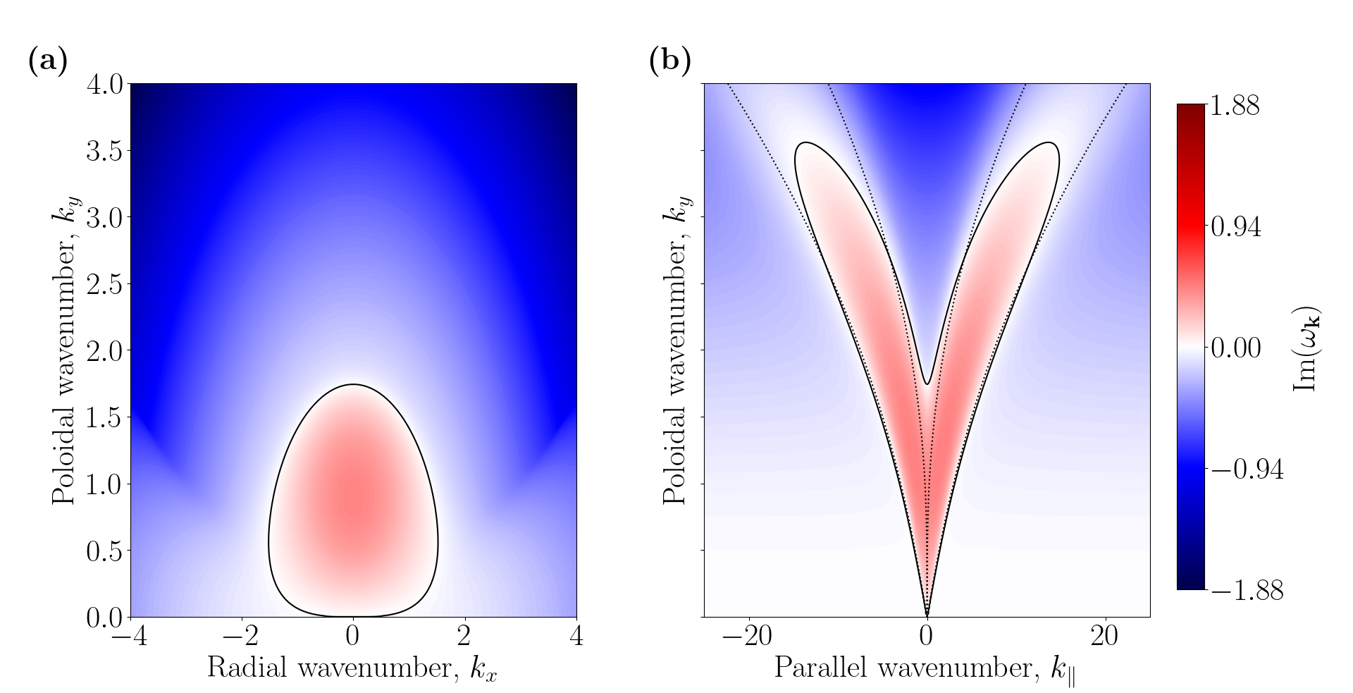
Figure 2: A visualisation of the linear growth rate, ${\text{Im}{\mathopen{}\mathclose{{}\left(\omega_{\boldsymbol{k}}}\right)}}$, given by eq. 20, for $\kappa_{T}=1$ and $\chi=0.1$. (a) The linear growth rate in the $k_{\parallel}=0$ plane. This is the 2D cITG instability that we dealt with in Ivanov et al. (2020). (b) The linear growth rate in the $k_{x}=0$ plane (where it is largest). The solid black lines denote the marginal modes with ${\text{Im}{\mathopen{}\mathclose{{}\left(\omega_{\boldsymbol{k}}}\right)}}=0$. The dotted lines outline the region of unstable collisionless ($\chi=0$), pure-slab ($L_{B}^{-1}=0$) modes, given by eq. 33.

Equations eq. 11–eq. 13 support two distinct types of linear instability, viz., cITG and sITG. The former was studied by Ivanov et al. (2020) and describes the linearly unstable 2D modes. In order to investigate the stability of the 3D modes, we drop the nonlinear terms in eq. 11–eq. 13 and look for Fourier modes $\varphi,T,{u}\propto\exp\mathopen{}\mathclose{{}\left(-i\omega_{\boldsymbol{k}}t+i{\boldsymbol{k}}\bcdot{\boldsymbol{r}}}\right)$, where ${\text{Re}{\mathopen{}\mathclose{{}\left(\omega_{\boldsymbol{k}}}\right)}}$, ${\text{Im}{\mathopen{}\mathclose{{}\left(\omega_{\boldsymbol{k}}}\right)}}$, and ${\boldsymbol{k}}=(k_{x},k_{y},k_{\parallel})$ are the real frequency, growth rate, and wavenumber of the mode, respectively. The dispersion relation can be written as

$$({-i\omega_{\boldsymbol{k}}}+s{k_{\perp}^{2}})D_{2D}+\frac{k_{\parallel}^{2}}{1+{k_{\perp}^{2}}}\mathopen{}\mathclose{{}\left({-i\omega_{\boldsymbol{k}}}+\chi{k_{\perp}^{2}}-i\kappa_{T}k_{y}}\right)=0,$$ (20)

where the 2D dispersion relation is given by

$$D_{2D}\equiv({-i\omega_{\boldsymbol{k}}}+A)({-i\omega_{\boldsymbol{k}}}+B-iC)-fAB+igAC=0,$$ (21)

$$A=\chi k_{\perp}^{2},\quad B=\frac{a\chi k_{\perp}^{4}}{1+k_{\perp}^{2}},\quad C=k_{y}\frac{1+\kappa_{T}k_{\perp}^{2}}{1+k_{\perp}^{2}},\quad f=\frac{\kappa_{T}k_{y}^{2}}{a\chi^{2}k_{\perp}^{6}},\quad g=\frac{b\kappa_{T}k_{\perp}^{2}}{1+\kappa_{T}k_{\perp}^{2}}.$$ (22)

An example of the solutions of eq. 20 is given in fig. 2. It is evident that eq. 20 is too complicated for a general analytical solution. Thus, we will limit our discussion here to several important limits.

3.1 Stable waves

Setting $\kappa_{T}=0$ and $\chi=0$ eliminates the linear instability and damping. The dispersion relation eq. 20 reduces to

$$(1+{k_{\perp}^{2}})\omega_{\boldsymbol{k}}^{2}+k_{y}\omega_{\boldsymbol{k}}-k_{\parallel}^{2}=0,$$ (23)

with solutions

$$\omega_{\boldsymbol{k}}=\frac{-k_{y}\pm\sqrt{k_{y}^{2}+4k_{\parallel}^{2}(1+{k_{\perp}^{2}})}}{2(1+{k_{\perp}^{2}})}.$$ (24)

In the limit $k_{\parallel}\ll k_{y}$ (which, in terms of dimensional wavenumbers, corresponds to $k_{\parallel}L_{B}\ll k_{y}\rho_{s}$), we find the familiar two-dimensional drift waves $\omega_{\boldsymbol{k}}=-k_{y}/(1+{k_{\perp}^{2}})$ that result from the magnetic drift. The opposite limit, $k_{\parallel}\gg k_{y}$, corresponds to equally familiar ion sound waves, modified by ion finite-Larmor-radius (FLR) effects: ${\omega_{\boldsymbol{k}}=k_{\parallel}/\sqrt{1+{k_{\perp}^{2}}}}$. We can undo the normalisations eq. 10 to verify that this is the usual dispersion for the ion sound waves in terms of the dimensional wavenumbers $k_{\parallel}$ and $k_{\perp}$:

$$\omega_{\boldsymbol{k}}=\pm\frac{c_{s}k_{\parallel}}{\sqrt{1+{k_{\perp}^{2}}\rho_{s}^{2}}}.$$ (25)

We now briefly recap the 2D cITG instability before turning to the $k_{\parallel}\neq 0$ sITG.

3.2 Curvature-driven ITG modes

3.2.1 Instability in 2D

The dispersion relation for the unstable 2D ($k_{\parallel}=0$) modes is eq. 21. These modes were studied carefully in Ivanov et al. (2020); let us recap some important points.

The 2D modes exist at large perpendicular scales, viz., $k_{\perp}<\text{min}\{k_{\perp,\text{max,FLR}},k_{\perp,\text{max},\chi}\}$, where the collisionless and collisional cut-offs are given by

$$k_{\perp,\text{max,FLR}}^{2}=\frac{1+2\sqrt{\kappa_{T}}}{\kappa_{T}},\quad k_{\perp,\text{max},\chi}^{2}=\sqrt{\frac{\kappa_{T}}{a\chi^{2}}},$$ (26)

respectively. As shown in Ivanov et al. (2020), the Dimits threshold in 2D satisfies $\kappa_{T}\sim\chi$. Here, however, we shall be interested in the strongly driven limit of $\kappa_{T}\gg\chi$ and $\kappa_{T}\gg 1$, for which a saturated state exists only in 3D. In this limit, eq. 26 tells us that the cITG modes exist at (and below) wavenumbers

$$k_{\perp}\sim k_{\perp,\text{max,FLR}}\sim\kappa_{T}^{-1/4}\ll 1.$$ (27)

Solving eq. 21 shows that these modes also satisfy

$${\text{Re}{\mathopen{}\mathclose{{}\left(\omega_{\boldsymbol{k}}}\right)}}\sim{\text{Im}{\mathopen{}\mathclose{{}\left(\omega_{\boldsymbol{k}}}\right)}}\sim\kappa_{T}^{1/4}.$$ (28)

3.2.2 $k_{\parallel}\neq 0$ corrections

Let us now see how $k_{\parallel}\neq 0$ affects the strongly driven modes at the curvature-driven scales $k_{\perp}\sim\kappa_{T}^{-1/4}\ll 1$. At these large perpendicular scales, the effects of collisions are negligible, so we may set $\chi=0$. Note that the scaling $k_{\perp}\sim\kappa_{T}^{-1/4}\ll 1$ implies $\kappa_{T}k_{\perp}^{2}\sim\sqrt{\kappa_{T}}\gg 1$, in which case the dispersion eq. 20 becomes

$$\omega_{\boldsymbol{k}}\mathopen{}\mathclose{{}\left[\omega_{\boldsymbol{k}}\mathopen{}\mathclose{{}\left(\omega_{\boldsymbol{k}}+\kappa_{T}k_{\perp}^{2}k_{y}}\right)+\kappa_{T}k_{y}^{2}}\right]=k_{\parallel}^{2}\mathopen{}\mathclose{{}\left(\omega_{\boldsymbol{k}}+\kappa_{T}k_{y}}\right),$$ (29)

where the dispersion relation for the curvature-driven 2D modes is the expression in the square brackets on the left-hand side. Using the results in section 3.2.1, we can estimate that for these modes, the left-hand and right-hand sides of eq. 29 satisfy

$$\omega_{\boldsymbol{k}}\mathopen{}\mathclose{{}\left[\omega_{\boldsymbol{k}}\mathopen{}\mathclose{{}\left(\omega_{\boldsymbol{k}}+\kappa_{T}k_{\perp}^{2}k_{y}}\right)+\kappa_{T}k_{y}^{2}}\right]\sim\kappa_{T}^{3/4},\quad k_{\parallel}^{2}\mathopen{}\mathclose{{}\left(\omega_{\boldsymbol{k}}+\kappa_{T}k_{y}}\right)\sim k_{\parallel}^{2}\kappa_{T}^{3/4}.$$ (30)

We can then conclude that for $k_{\parallel}\ll 1$, the solutions are essentially 2D, i.e., the dispersion relation eq. 29 is well-approximated by eq. 21, whereas $k_{\parallel}\gg 1$ is expected to introduce qualitative changes to the modes. Let us now investigate the $k_{\parallel}\gg 1$ sITG instability.

3.3 Collisionless slab-ITG modes

Let us investigate the linear instability of eq. 11–eq. 13 in the absence the magnetic-gradient term $-\partial_{y}(\varphi+T)$ in eq. 11. We shall see shortly when this is appropriate. For now, we limit ourselves to the collisionless ($\chi=0$) regime (see also section 3.4 and appendix C). Then, eq. 20 becomes

$$\mathopen{}\mathclose{{}\left(\hat{\omega}_{\boldsymbol{k}}^{2}-\frac{\hat{k}_{\parallel}^{2}}{1+k_{\perp}^{2}}}\right)\mathopen{}\mathclose{{}\left(\hat{\omega}_{\boldsymbol{k}}+1}\right)=\frac{2k_{\perp}^{2}\hat{\gamma}_{\boldsymbol{k}}^{2}\hat{\omega}_{\boldsymbol{k}}^{2}}{1+k_{\perp}^{2}},$$ (31)

where we have defined $\omega_{\boldsymbol{k}}\equiv\kappa_{T}k_{y}\hat{\omega}_{\boldsymbol{k}}$, $k_{\parallel}\equiv\kappa_{T}k_{y}\hat{k}_{\parallel}$, and $\hat{\gamma}_{\boldsymbol{k}}^{2}\equiv 1/2k_{\perp}^{2}$. The last of these may seem like an inconvenience now, but will make the following analysis more easily generalisable for our needs in section 4. Since eq. 31 is a real cubic in $\hat{\omega}_{\boldsymbol{k}}$, it either has three real solutions, so all linear modes are stable waves, or one real and two complex solutions, in which case one of the complex solutions has a positive imaginary part and thus corresponds to a linearly unstable mode. It can be shown (see appendix B) that eq. 31 has complex solutions if and only if $\hat{\gamma}_{\boldsymbol{k}}^{2}>0$ and $\hat{k}_{\parallel}^{2}\in(\hat{k}_{\parallel,-}^{2},\hat{k}_{\parallel,+}^{2})$, where

$$\hat{k}_{\parallel,\pm}^{2}=\frac{k_{\perp}^{4}+10k_{\perp}^{2}\hat{\gamma}_{\boldsymbol{k}}^{2}(1+k_{\perp}^{2})+k_{\perp}^{2}(4-k_{\perp}^{2}\hat{\gamma}_{\boldsymbol{k}}^{2})+2\pm k_{\perp}\hat{\gamma}_{\boldsymbol{k}}\mathopen{}\mathclose{{}\left[4(1+k_{\perp}^{2})+k_{\perp}^{2}\hat{\gamma}_{\boldsymbol{k}}^{2}}\right]^{3/2}}{2(1+k_{\perp}^{2})}.$$ (32)

Substituting $\hat{\gamma}_{\boldsymbol{k}}^{2}=1/2k_{\perp}^{2}$ yields

$$\hat{k}_{\parallel,\pm}^{2}=\frac{9}{8(1+k_{\perp}^{2})}\mathopen{}\mathclose{{}\left[\frac{8k_{\perp}^{4}}{9}+4k_{\perp}^{2}+3\pm 3\mathopen{}\mathclose{{}\left(1+\frac{8k_{\perp}^{2}}{9}}\right)^{3/2}}\right].$$ (33)

The marginal modes, i.e., those on the boundary between unstable and oscillatory modes, are given by $\hat{k}_{\parallel}^{2}=\hat{k}_{\parallel,\pm}^{2}$; these are shown in fig. 3. We now consider two distinct asymptotic limits of eq. 33: $k_{\perp}\ll 1$ and $k_{\perp}\gg 1$.

3.3.1 Large-scale slab-ITG instability: $k_{\perp}\ll 1$ modes

To lowest order in $k_{\perp}\ll 1$, eq. 31 simplifies to

$$\hat{\omega}_{\boldsymbol{k}}^{3}-\hat{k}_{\parallel}^{2}\hat{\omega}_{\boldsymbol{k}}-\hat{k}_{\parallel}^{2}=0.$$ (34)

This is the well-known sITG dispersion relation without FLR effects and in the absence of a density gradient (Cowley et al., 1991). In this limit, the instability boundaries eq. 33 become

$$\hat{k}_{\parallel,-}=\frac{2}{3\sqrt{3}}k_{\perp}^{3}+\mathcal{O}\mathopen{}\mathclose{{}\left(k_{\perp}^{5}}\right),\quad\hat{k}_{\parallel,+}=\frac{3\sqrt{3}}{2}+\frac{\sqrt{3}}{4}k_{\perp}^{2}+\mathcal{O}\mathopen{}\mathclose{{}\left(k_{\perp}^{4}}\right).$$ (35)

For small $\hat{k}_{\parallel}$, the linearly unstable solution of eq. 34 is $\hat{\omega}_{\boldsymbol{k}}\approx|\hat{k}_{\parallel}^{2/3}|(-1+i\sqrt{3})/2$. Thus, the linear growth rate for small $\hat{k}_{\parallel}$, or $k_{\parallel}\ll\kappa_{T}k_{y}$, is

$${\text{Im}{\mathopen{}\mathclose{{}\left(\omega_{\boldsymbol{k}}}\right)}}\approx\frac{\sqrt{3}}{2}\mathopen{}\mathclose{{}\left(\kappa_{T}k_{y}k_{\parallel}^{2}}\right)^{1/3}.$$ (36)

This is the most widely recognised expression for the sITG growth rate at long wavelengths, however, it is not the fastest-growing mode at $k_{y}\ll 1$. From eq. 35, we know that eq. 34 has ${\text{Im}{(\hat{\omega}_{\boldsymbol{k}})}}>0$ solutions up to $\hat{k}_{\parallel}=\mathcal{O}(1)$, or $k_{\parallel}\sim\kappa_{T}k_{y}$. The growth rate of these modes evidently satisfies ${\text{Im}{(\hat{\omega}_{\boldsymbol{k}})}}=\mathcal{O}(1)$, or ${\text{Im}{(\omega_{\boldsymbol{k}})}}\sim\kappa_{T}k_{y}$.

We are now able to confirm that neglecting the magnetic drift in deriving eq. 31, and hence eq. 34, was appropriate. As we saw in section 3.2.1, the strongly driven ($\kappa_{T}\gg 1$) 2D cITG modes satisfy $k_{y}\sim\kappa_{T}^{-1/4}$. At these wavenumbers, the sITG modes exist at scales $k_{\parallel}\sim\kappa_{T}^{3/4}\gg 1$ (as expected and assumed) and have a growth rate ${\text{Im}{(\omega_{\boldsymbol{k}})}}\sim\kappa_{T}k_{y}\sim\kappa_{T}^{3/4}$, which is asymptotically larger than the growth rate ${\text{Im}{(\omega_{\boldsymbol{k}})}}\sim\kappa_{T}^{1/4}$ of the cITG modes.

3.3.2 Small-scale slab-ITG instability: $k_{\perp}\gg 1$ modes

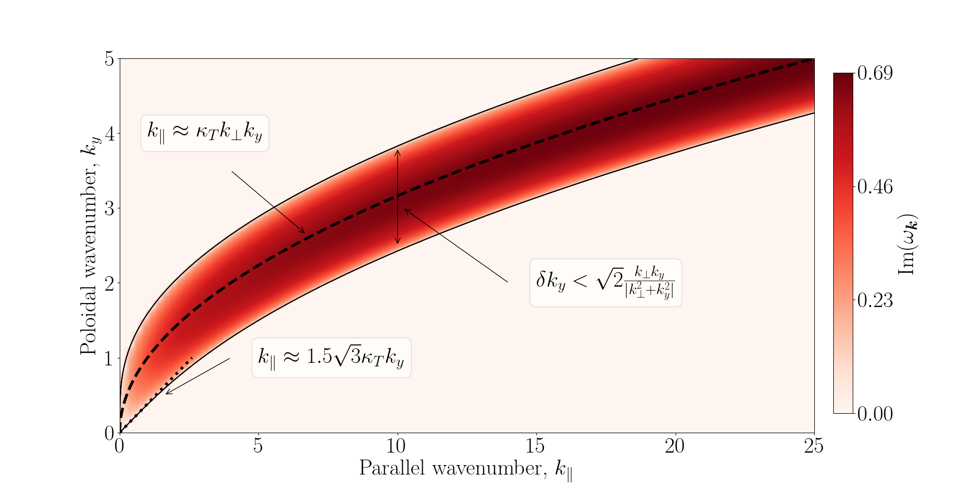
Figure 3: Linear growth rates for the sITG instability (without the magnetic drift) as a function of parallel ($k_{\parallel}$) and poloidal ($k_{y}$) wavenumbers for $k_{x}=0$, $\kappa_{T}=1$, $\chi=0$. The growth rate along the $k_{\parallel}=\kappa_{T}k_{\perp}k_{y}$ line converges to $\kappa_{T}/\sqrt{2}\approx 0.7$ for large $k_{\parallel}$. The solid black lines are the instability boundary given by eq. 33.

Expanding eq. 32 for $k_{\perp}\gg 1$ and using $\hat{\gamma}_{\boldsymbol{k}}=\mathcal{O}\mathopen{}\mathclose{{}\left(k_{\perp}^{-1}}\right)$, we find

$$\hat{k}_{\parallel,\pm}=k_{\perp}(1\pm 2\hat{\gamma}_{\boldsymbol{k}})+\mathcal{O}\mathopen{}\mathclose{{}\left(k_{\perp}^{-1}}\right).$$ (37)

Therefore, at small perpendicular scales, the sITG is localised at $\hat{k}_{\parallel}=\pm k_{\perp}$, or, equivalently, at

$$k_{\parallel}\approx\pm\kappa_{T}k_{y}k_{\perp}.$$ (38)

In terms of the dimensional wavenumbers, eq. 38 tells us that this instability is localised at $k_{\parallel}L_{B}/2\approx\pm\kappa_{T}k_{y}k_{\perp}\rho_{s}^{2}$, or, equivalently, $k_{\parallel}L_{T}\approx\pm k_{y}k_{\perp}\rho_{i}^{2}$. For $\hat{\gamma}_{\boldsymbol{k}}^{2}=1/2k_{\perp}^{2}$, eq. 37 is

$$\hat{k}_{\parallel,\pm}=k_{\perp}\pm\sqrt{2}+\mathcal{O}\mathopen{}\mathclose{{}\left(k_{\perp}^{-1}}\right),$$ (39)

which implies, for the unstable modes,

$$\mathopen{}\mathclose{{}\left\lvert\hat{k}_{\parallel}-k_{\perp}}\right\rvert=\mathopen{}\mathclose{{}\left\lvert\frac{k_{\parallel}}{\kappa_{T}k_{y}}-k_{\perp}}\right\rvert<\sqrt{2}.$$ (40)

We can also find the $k_{y}$ width of the region of instability at fixed $k_{\parallel}$. Substituting $k_{y}=k_{\parallel}/\kappa_{T}k_{\perp}+\delta k_{y}$ into eq. 40 and expanding for $\delta k_{y}\ll k_{y}$, we find

$$|\delta k_{y}|<\sqrt{2}\frac{k_{\perp}k_{y}}{|k_{\perp}^{2}+k_{y}^{2}|}\leq\frac{\sqrt{2}}{2}.$$ (41)

To find the growth rate, consider the $k_{\perp}\gg 1$ limit of eq. 31 and set $\hat{k}_{\parallel}=\pm k_{\perp}+\delta\hat{k}_{\parallel}$ and $\hat{\omega}_{\boldsymbol{k}}=-1+\delta\hat{\omega}_{\boldsymbol{k}}$, where $\delta\hat{\omega}_{\boldsymbol{k}}\sim\delta\hat{k}_{\parallel}/k_{\perp}\sim\mathcal{O}(k_{\perp}^{-1})\ll 1$. Keeping terms of order up to $\mathcal{O}(k_{\perp}^{-2})$, eq. 31 becomes

$$\mathopen{}\mathclose{{}\left(\delta\hat{\omega}_{\boldsymbol{k}}\pm\frac{\delta\hat{k}_{\parallel}}{k_{\perp}}}\right)\delta\hat{\omega}_{\boldsymbol{k}}+\hat{\gamma}_{\boldsymbol{k}}^{2}\approx 0\implies\delta\hat{\omega}_{\boldsymbol{k}}\approx-\frac{\delta\hat{k}_{\parallel}}{2k_{\perp}}\pm\sqrt{\frac{\delta\hat{k}_{\parallel}^{2}}{4k_{\perp}^{2}}-\hat{\gamma}_{\boldsymbol{k}}^{2}}.$$ (42)

Thus, in agreement with eq. 40, the instability exists only for $|\delta\hat{k}_{\parallel}|<2k_{\perp}\hat{\gamma}_{\boldsymbol{k}}$, and its growth rate is

$${\text{Im}{\mathopen{}\mathclose{{}\left(\hat{\omega}_{\boldsymbol{k}}}\right)}}\approx\sqrt{\hat{\gamma}_{\boldsymbol{k}}^{2}-\frac{\delta\hat{k}_{\parallel}^{2}}{4k_{\perp}^{2}}}.$$ (43)

The maximum growth rate is then achieved for $\delta\hat{k}_{\parallel}=0$, i.e., at $k_{\parallel}=\pm\kappa_{T}k_{y}k_{\perp}$, and is given by ${\text{Im}{\mathopen{}\mathclose{{}\left(\hat{\omega}_{\boldsymbol{k}}}\right)}}\approx\hat{\gamma}_{\boldsymbol{k}}$. Since $\hat{\gamma}_{\boldsymbol{k}}^{2}=1/2k_{\perp}^{2}$, this is

$${\text{Im}{\mathopen{}\mathclose{{}\left(\omega_{\boldsymbol{k}}}\right)}}\approx\frac{\kappa_{T}k_{y}}{\sqrt{2}k_{\perp}}\leq\frac{\kappa_{T}}{\sqrt{2}}.$$ (44)

The characteristics of the small-scale sITG instability are summarised in fig. 3.

Note that for $\kappa_{T}\gg 1$, the linear growth rate eq. 44 of the small-scale sITG modes scales as $\mathcal{O}(\kappa_{T})$ and, therefore, dominates both the curvature-driven modes (section 3.2.1) and the large-scale slab modes (section 3.3.1). This time-scale separation will prove critical for the saturation of strongly driven turbulence (see section 4.2.2).

Finally, an important feature of the $k_{\perp}\gg 1$ sITG modes is the approximate relation $T\approx-\varphi$, or equivalently, $p/\varphi\ll 1$, where $p=\varphi+T$ is the perturbed pressure. Indeed, using eq. 12 and eq. 42, we find

$$\frac{T_{\boldsymbol{k}}}{\varphi_{\boldsymbol{k}}}=\frac{\kappa_{T}k_{y}}{\omega_{\boldsymbol{k}}}=\frac{1}{\hat{\omega}_{\boldsymbol{k}}}=-1+\frac{\delta\hat{k}_{\parallel}}{2k_{\perp}}-i\sqrt{\hat{\gamma}_{\boldsymbol{k}}^{2}-\frac{\delta\hat{k}_{\parallel}^{2}}{4k_{\perp}^{2}}}+\mathcal{O}\mathopen{}\mathclose{{}\left(k_{\perp}^{-2}}\right)$$ (45)

for the modes with ${\text{Im}{\mathopen{}\mathclose{{}\left(\hat{\omega}_{\boldsymbol{k}}}\right)}}>0$. Thus, these modes generally have $p_{\boldsymbol{k}}/\varphi_{\boldsymbol{k}}\sim\mathcal{O}(k_{\perp}^{-1})\ll 1$, while the most unstable of them ($\delta\hat{k}_{\parallel}=0$) satisfy $p_{\boldsymbol{k}}/\varphi_{\boldsymbol{k}}\sim\mathcal{O}(k_{\perp}^{-2})$ and ${\text{Re}{\mathopen{}\mathclose{{}\left(T_{\boldsymbol{k}}/\varphi_{\boldsymbol{k}}}\right)}}=-1+\mathcal{O}(k_{\perp}^{-2})$. This relationship between $T_{\boldsymbol{k}}$ and $\varphi_{\boldsymbol{k}}$ will allow us to identify the sITG modes in the saturated state, and will prove useful in understanding their role in maintaining the Dimits state (see section 4.2.1 and section 4.2.5).

3.4 Mechanism of the small-scale slab-ITG instability

The analysis in section 3.3.2 is somewhat physically opaque. To get a better grasp of the small-scale sITG modes, we can consider the problem from a slightly different angle. Let us subtract the Laplacian $\nabla_{\perp}^{2}$ of eq. 12 from eq. 11 and rewrite the linear part of the system eq. 11–eq. 13 as

$$\partial_{t}\mathopen{}\mathclose{{}\left(\varphi^{\prime}-\nabla_{\perp}^{2}\varphi}\right)+\partial_{\parallel}{u}-\partial_{y}p+\kappa_{T}\partial_{y}\nabla_{\perp}^{2}\varphi+\chi\nabla_{\perp}^{4}\mathopen{}\mathclose{{}\left[(a+b)\varphi-bp}\right]=0,$$ (46)

$$-\partial_{t}\nabla_{\perp}^{2}p+\partial_{\parallel}{u}-\partial_{y}p+\chi{\boldsymbol{\nabla}}_{\perp}^{4}(1-b)p=-\partial_{t}\varphi^{\prime}-\chi{\boldsymbol{\nabla}}_{\perp}^{4}(a+b-1)\varphi,$$ (47)

$$\partial_{t}{u}+\partial_{\parallel}p-s\chi\nabla_{\perp}^{2}{u}=0,$$ (48)

where $p=\varphi+T$ is the pressure perturbation. Let us first concentrate on the $\chi=0$ case, viz.,

$$\partial_{t}\mathopen{}\mathclose{{}\left(\varphi^{\prime}-\nabla_{\perp}^{2}\varphi}\right)+\partial_{\parallel}{u}-\partial_{y}p+\kappa_{T}\partial_{y}\nabla_{\perp}^{2}\varphi=0,$$ (49)

$$-\partial_{t}\nabla_{\perp}^{2}p+\partial_{\parallel}{u}-\partial_{y}p=-\partial_{t}\varphi^{\prime},$$ (50)

$$\partial_{t}{u}+\partial_{\parallel}p=0.$$ (51)

Observe that the term $\partial_{t}\varphi^{\prime}$ on the right-hand side of eq. 50 is asymptotically small in the $k_{\perp}\gg 1$ limit. Indeed, had we approximated $\partial_{t}(1+k_{\perp}^{2})\varphi\approx\partial_{t}k_{\perp}^{2}\varphi$ in eq. 11, as we should have done for $k_{\perp}\gg 1$, the right-hand side of eq. 50 would have been zero. In this approximation, eq. 50 and eq. 51 decouple from eq. 49. Their dispersion relation coincides with the $k_{\perp}\gg 1$ limit of eq. 24, so eq. 50 and eq. 51 describe two propagating waves, independent of $\kappa_{T}$. Let us call these two modes ‘pressure waves’. The third mode is a $p={u}=0$ wave, described by eq. 49; its frequency in the $k_{\perp}\gg 1$ limit is $\omega_{\boldsymbol{k}}=-\kappa_{T}k_{y}$. We shall call this a ‘diamagnetic wave’ because the restoring force comes from the diamagnetic-drift term $\kappa_{T}\partial_{y}\nabla_{\perp}^{2}\varphi$ in eq. 49.

Since the diamagnetic and pressure waves have, in general, disparate frequencies, the small coupling term $-\partial_{t}\varphi^{\prime}$ in eq. 50 can indeed be neglected. However, if the frequencies of these modes happen to coincide, i.e., if they are in resonance, the small coupling term can no longer be neglected. Using eq. 24 for the frequency of the pressure waves and $\omega_{\boldsymbol{k}}=-\kappa_{T}k_{y}$ for the diamagnetic wave, we find that such a resonance occurs when $k_{\parallel}=\kappa_{T}k_{\perp}k_{y}$, assuming $k_{\perp}\gg 1$. Thus, the instability condition eq. 38 for collisionless small-scale sITG modes is the resonance condition for the two types of linear modes in the system, viz., pressure waves and diamagnetic waves.

Let us now restore $\chi\neq 0$. Then, eq. 47 shows that for $a+b\neq 1$ (as is generally the case), there is a second coupling mechanism, via the term $\chi{\boldsymbol{\nabla}}_{\perp}^{4}(a+b-1)\varphi$. For $\omega_{\boldsymbol{k}}\sim\kappa_{T}k_{y}$, this term is comparable to the collisionless-coupling term $\partial_{t}\varphi^{\prime}$ when $\omega_{\boldsymbol{k}}\sim\kappa_{T}k_{y}\sim\chi k_{\perp}^{4}$, i.e., when

$$k_{\perp}\sim\mathopen{}\mathclose{{}\left(\frac{\kappa_{T}}{\chi}}\right)^{1/3}\equiv k_{\chi},$$ (52)

assuming $k_{\perp}\sim k_{y}$. We find that $k_{\chi}$ is the perpendicular scale at which the collisionless results of section 3.3.2 are no longer valid as the effects of finite $\chi$ can no longer be neglected. Naïvely, one might expect that for $k_{\perp}>k_{\chi}$, collisions will act to damp the sITG instability. However, this turns out not to be the case, and, in fact, the coupling term $\chi{\boldsymbol{\nabla}}_{\perp}^{4}(a+b-1)\varphi$ can mediate a new collisional ITG instability ($\chi$ITG) for $k_{\perp}\gtrsim k_{\chi}$ in the absence of the collisionless coupling term $\partial_{t}\varphi^{\prime}$. However, it turns out that in order for $\chi$ITG to be non-negligible compared to sITG, very large temperature gradients are required, viz., $\kappa_{T}/\chi\gtrsim 830$. Numerically, we shall not investigate such large gradients, so the $\chi$ITG instability will not be relevant for us. The detailed treatment of the $\chi$ITG instability has been relegated to appendix C.

4 Nonlinear states of low and high transport

We now proceed to study the nonlinear saturated state of eq. 11–eq. 13. We solve these equations using an enhanced version of the code used in Ivanov et al. (2020), whereby eq. 11–eq. 13 are solved using a pseudo-spectral algorithm in a triply periodic box of dimensions $L_{x}$, $L_{y}$, and $L_{\parallel}$. The linear terms are integrated implicitly in time, while the nonlinear terms are integrated explicitly using the Adams–Bashforth three-step method. This integration scheme is similar to the one implemented in the popular GK code GS2 (Kotschenreuther et al., 1995; Dorland et al., 2000). As the 3D model has no dissipation terms that depend on $k_{\parallel}$, we usually include small (compared to the collisional dissipation) parallel hyperviscosity of the form $\nu k_{\parallel}^{4}$. It is incorporated in the equations by replacing $\partial_{t}\mapsto\partial_{t}+\nu k_{\parallel}^{4}$ for all three fields in the model. The value of $\nu$ is typically chosen to give a maximum parallel hyperviscosity of $10\%$ of $\chi k_{\perp,\text{largest}}^{2}$, where $k_{\perp,\text{largest}}$ is the largest $k_{\perp}$ included the simulation. This form of hyperviscosity effectively subtracts $\nu k_{\parallel}^{4}$ from the growth rate of every mode, but does not alter the linear mode structure, i.e., it does not influence the ratio of Reynolds to diamagnetic stresses given by ${\text{Re}{\mathopen{}\mathclose{{}\left(T_{\boldsymbol{k}}/\varphi_{\boldsymbol{k}}}\right)}}$ (see section 4.1 and section 4.2.5). Thus, it dissipates energy without perturbing the saturated state either towards or away from the Dimits regime.

Recall that the 2D model has two distinct nonlinear states — a Dimits regime, where saturation is achieved with the aid of strong ZFs that quench the cITG instability by shearing the perturbations it produces, and a blow-up regime, where no finite-amplitude saturation is achieved, but amplitudes continue to grow exponentially indefinitely (or at least until numerical efforts become futile). This unphysical blow up is arguably the main limitation of the 2D model, and there are good reasons to believe that it is a consequence of the $k_{\parallel}=0$ restriction (see §4.5 of Ivanov et al., 2020). This will indeed be corroborated below as we find that the 3D model is able to saturate for all values of $\kappa_{T}$ and $\chi$ that we have investigated numerically.

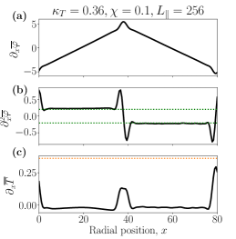
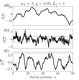
Figure 4: Example of instantaneous radial profiles of perturbations in the 3D Dimits state for $L_{x}=L_{y}=80$: (a) ZF, (b) zonal shear, (c) zonal temperature gradient. Example of instantaneous radial profiles in strong turbulence: (d) ZF, (e) zonal shear, (f) zonal temperature gradient. The dotted green lines in (b) and (e) are the largest linear growth rates for the respective simulations. The dotted orange lines in (c) and (f) show the value of $\kappa_{T}$, which is equal to minus the normalised equilibrium temperature gradient. Just as in 2D, the zonal shear in the Dimits state is determined by the largest linear growth rate. Strongly turbulent ZFs do not have regions of coherent shear.

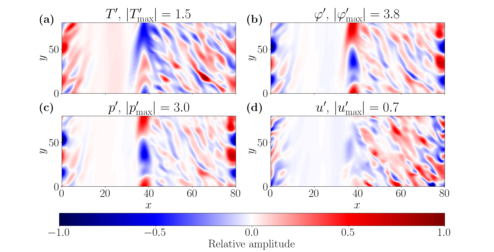
Figure 5: Snapshots of the perturbed nonzonal (a) temperature $T^{\prime}$, (b) potential $\varphi^{\prime}$, (c) pressure $p^{\prime}=\varphi^{\prime}+T^{\prime}$, and (d) parallel velocity ${u}^{\prime}$ in the 3D Dimits state. The colour scale is relative to the maximum absolute amplitude in each panel (given in the panels’ titles). We see that ferdinons carry a ${u}$ perturbation, as well as $T$ and $\varphi$ perturbations. A more detailed view of one of the ferdinons is shown in fig. 7. These snapshots are from the same simulation as figures 4a–c.

At low collisionality (which can be argued to be the most relevant case, at least for core turbulence, see Ivanov et al., 2020), the Dimits regime of the 3D model is strikingly similar to its 2D counterpart. The saturated state is dominated by quasi-static triangular ZFs that break up the radial domain into regions (shear zones) of constant zonal shear, where turbulence is sheared and thus suppressed (see figures 4a–c). Localised patches of turbulence remain present at the turning points of the ZFs, where the zonal shear vanishes.

Periodically, when viscosity has eroded the ZFs and their ability to suppress turbulence has diminished, turbulent bursts are triggered. Just as in 2D, these bursts are foreshadowed by an instability located at the ZF maxima and by the appearance of localised travelling structures produced by this instability (‘ferdinons’, discovered by van Wyk et al. 2016, 2017 in GK simulations with external flow shear). An example of a turbulent burst in the 3D model is shown in fig. 5. It is visually indistinguishable from a burst in 2D when viewed as a cross section in the $(x,y)$ plane. We shall discuss the 3D structure of the Dimits regime in detail in section 4.1.

The crucial qualitative change in physics that allowing 3D perturbations brings about is the sITG instability. Recall that the collisionless small-scale sITG modes live at wavenumbers up to $k_{\chi}\sim(\kappa_{T}/\chi)^{1/3}$ (see section 3.4). This is in stark contrast with the behaviour of the 2D cITG modes whose cut-off wavenumber eq. 26 scales as $k_{\perp,\text{2D cut-off}}\sim\kappa_{T}^{-1/4}$ (see also §2.6.1. of Ivanov et al., 2020). Moreover, the maximal growth rate of the sITG modes eq. 44 scales as ${\text{Im}{\mathopen{}\mathclose{{}\left(\omega_{\boldsymbol{k}}}\right)}}\sim\kappa_{T}$, while that of the cITG modes eq. 28 satisfies ${\text{Im}{\mathopen{}\mathclose{{}\left(\omega_{{\boldsymbol{k}},\text{2D}}}\right)}}\sim\kappa_{T}^{1/4}$. This implies that there is a natural scale separation between slow, large-scale curvature-driven modes and fast, small-scale sITG modes. Crucially, this scale separation allows small-scale turbulence to be driven both by the equilibrium gradients and by the gradients associated with the large-scale 2D modes (which are themselves generated by the cITG instability). In fact, as we shall see in section 4.2, the latter type of driving dominates in the saturated state to such an extent that the equilibrium temperature gradient can be turned off for the $k_{\parallel}\neq 0$ modes and the saturated state remains largely unchanged. In other words, the sITG modes are ‘parasitic’ modes, a type of 3D ‘secondary’ instability of the 2D cITG modes.

Most importantly, in the Dimits state, the small-scale instability can be shown always to favour strong, coherent ZFs. It does so in two ways: by providing an effective positive thermal diffusion for the large-scale modes that would otherwise destabilise the ZFs in 2D (see section 4.2.4), and by generating momentum transport that is beneficial for the ZFs (i.e., a negative turbulent viscosity for the zonal flow, see section 4.2.5). This makes the 3D Dimits state much more resilient than the 2D one. In fact, we find that the 3D system stays in a Dimits state regardless of the values of the parameters $\kappa_{T}$ and $\chi$, provided the domain is ‘sufficiently 3D’, i.e., provided $L_{\parallel}$ is large enough and that our numerical simulations have sufficient parallel resolution to resolve the sITG modes (see section 4.3).

We now recap the physical mechanism that gives rise to the Dimits regime and also discuss any qualitative and quantitative changes that the 3D physics brings about. Then, in section 4.2, we turn to the small-scale sITG instability and its consequences for the saturated state. Finally, in section 4.3, we examine the circumstances that can prevent the system from establishing a Dimits state and force it into the strongly turbulent regime.

4.1 Dimits regime

4.1.1 The 2D picture

Recall that the 2D Dimits transition is a sharp transition from a finite-amplitude saturated state with strong ZFs to a ‘blow-up’ state dominated by ever-growing streamers (Ivanov et al., 2020). The key to understanding this is the equation for the zonal electrostatic potential

$$\partial_{t}\overline{\varphi}+\Pi_{\varphi}+\Pi_{T}+\Pi_{\chi}=0,$$ (53)

where

$$\Pi_{\varphi}\equiv-\overline{(\partial_{x}\varphi)(\partial_{y}\varphi)},\qquad\Pi_{T}\equiv-\overline{(\partial_{x}\varphi)(\partial_{y}T)},\qquad\Pi_{\chi}\equiv-\chi\partial_{x}^{2}\mathopen{}\mathclose{{}\left(a\overline{\varphi}-b\overline{T}}\right)$$ (54)

are the Reynolds, diamagnetic, and diffusive stresses, respectively. Equation eq. 53 describes how the ZFs are generated or eroded by turbulence (via the Reynolds and diamagnetic stresses, depending on their sign) and damped by collisional viscosity. We then consider a region of nearly constant zonal shear (a ‘shear zone’) of radial width $d$ and find that the integral of the total turbulent stress $\Pi_{t}=\Pi_{\varphi}+\Pi_{T}$ over such a region can be written as

$$\frac{1}{d}\int dx\Pi_{t}=-\sum_{\boldsymbol{k}}k_{x}k_{y}|\varphi_{\boldsymbol{k}}|^{2}\mathopen{}\mathclose{{}\left[1+{\text{Re}{\mathopen{}\mathclose{{}\left(\frac{T_{\boldsymbol{k}}}{\varphi_{\boldsymbol{k}}}}\right)}}}\right].$$ (55)

Thus, the effect of the mode with wavenumber ${\boldsymbol{k}}$ on the ZFs depends on the ratio ${\text{Re}{\mathopen{}\mathclose{{}\left(T_{\boldsymbol{k}}/\varphi_{\boldsymbol{k}}}\right)}}$. Namely, ${\text{Re}{\mathopen{}\mathclose{{}\left(T_{\boldsymbol{k}}/\varphi_{\boldsymbol{k}}}\right)}}<-1$ implies that the mode will destabilise the ZFs, while ${\text{Re}{\mathopen{}\mathclose{{}\left(T_{\boldsymbol{k}}/\varphi_{\boldsymbol{k}}}\right)}}>-1$ means that the mode will reinforce the ZFs. This observation is based on the fact that sheared (by the ZFs) turbulence is ‘tilted’ and the sign of $k_{x}k_{y}$ is correlated with the sign of the zonal shear in each shear zone. In Ivanov et al. (2020), we derived a simple estimate for the Dimits threshold at large $\kappa_{T}$ that was based on applying these ideas to the linear modes of the 2D system. More generally, we argued that the Dimits transition occurred at the threshold of a nonlinear version of the secondary instability — when sheared by ZFs, turbulence either reinforced these flows and thus a Dimits state was maintained (the Reynolds stress won), or it failed to do so (the diamagnetic stress won) and saturation had to be reached via a different route that did not rely on zonal shear. In the 2D case, no such alternative route for finite-amplitude saturation existed. This description of how a ZF-dominated state was maintained was demonstrated to be accurate by calculating the turbulent viscosity

$$\nu_{t}\equiv-\frac{\langle\int_{0}^{L_{x}}dx\ \Pi_{t}S\rangle_{\Delta t}}{\langle\int_{0}^{L_{x}}dx\ S^{2}\rangle_{\Delta t}}$$ (56)

in numerical simulations with an imposed static ZF profile; here $\langle\dots\rangle_{\Delta t}$ is a saturated-state time average and $S\equiv\partial_{x}^{2}\overline{\varphi}$ is the zonal shear. Essentially, $\nu_{t}$ is a measure of the correlation between the turbulent stress $\Pi_{t}$ and the zonal shear $S$. We found that $\nu_{t}<0$ on the Dimits side of the threshold, indicating that sheared turbulence was feeding the ZFs, which were shearing it. Accordingly, we also found $\nu_{t}>0$ beyond the threshold, implying that the turbulent stress was actively suppressing the ZFs.

4.1.2 The influence of $L_{\parallel}$ on the Dimits state

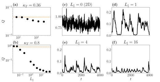
Figure 6: (a) Dependence of the time-averaged heat flux $Q$ on the parallel size of the box $L_{\parallel}$ for $\chi=0.1$, $L_{x}=L_{y}=80$, and $\kappa_{T}=0.36$. The orange dotted line shows the time-averaged heat flux for the 2D state ($L_{\parallel}=0$). (b) Same as (a), but with $\kappa_{T}=0.8$. (c)–(f) Time evolution of the heat flux $Q$ for $\kappa_{T}=0.8$, $\chi=0.1$, $L_{x}=80$, $L_{y}=80$ and four different values of $L_{\parallel}$ (notated on each panel). As $L_{\parallel}$ increases, the turbulent bursts become more frequent and less violent, and the time-averaged $Q$ drops.

Taking the limit $L_{\parallel}\to 0$ effectively restricts our model equations eq. 11–eq. 13 to 2D, and thus their saturated Dimits state converges to that of the 2D model. In figures 6a and 6b, we show what happens to the turbulent heat flux $Q$ with increasing $L_{\parallel}$ for two cases: far below the 2D Dimits threshold ($\kappa_{T}=0.36$, $\chi=0.1$), where turbulent bursts dominate the 2D state, and closer to it ($\kappa_{T}=0.8$, $\chi=0.1$), where the bursts start to overlap in time. As expected, if $L_{\parallel}$ is small enough, we recover the 2D results. As $L_{\parallel}$ increases, $Q$ converges in a monotonic way to a definite 3D value that is smaller than the 2D heat flux. Figures 6c–f show that, for larger values of $L_{\parallel}$, the turbulent bursts become more frequent, but shorter in duration and lower in amplitude. There are two effects responsible for this — parallel localisation of turbulence and the development of the ‘parasitic’ small-scale sITG modes.

Parallel localisation is inevitable because the turbulent nonzonal modes cannot propagate information infinitely quickly along the field lines. As we increase $L_{\parallel}$ away from 0, we see elongated nonzonal modes that eventually lose the ability to stay coherent along the field lines if $L_{\parallel}$ is large enough. Figure 7 shows that the typical Dimits-state ferdinons are not true 2D structures and develop a finite parallel extent if the parallel size of the box allows it. This is in contrast with the ZFs, which do stay perfectly coherent along the entire domain regardless of $L_{\parallel}$. This puts the ZFs at an advantage because the turbulent stresses in eq. 53 are parallel averages and so a turbulent burst that is localised to a fraction $\Delta L_{\parallel}/L_{\parallel}$ of the parallel extent of the box has its turbulent stress diminished by a factor of $\Delta L_{\parallel}/L_{\parallel}$. As we increase $L_{\parallel}$, every such localised burst provides a smaller restoring ‘kick’ to the ZFs and so it takes less time for the ZFs to decay to a level that permits the development of a new burst. The turbulent heat flux $Q$ is also a spatial average of the turbulent fields and it too is diminished for a localised burst. Thus, we expect smaller, more frequent bursts, and this is precisely what is observed. Note that the ability of ZFs to communicate infinitely fast along the field lines is a consequence of the asymptotic limit of small mass ratio and the modified adiabatic electron response eq. 1, which is itself due to the assumed infinitely fast parallel electron streaming. Therefore, the inclusion of kinetic electron effects in the equations would lead to qualitative changes for a large enough $L_{\parallel}$. Naturally, this is outside the scope of this work, but is certainly an important consideration for real devices.

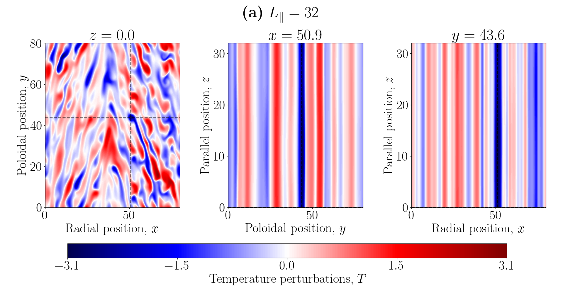
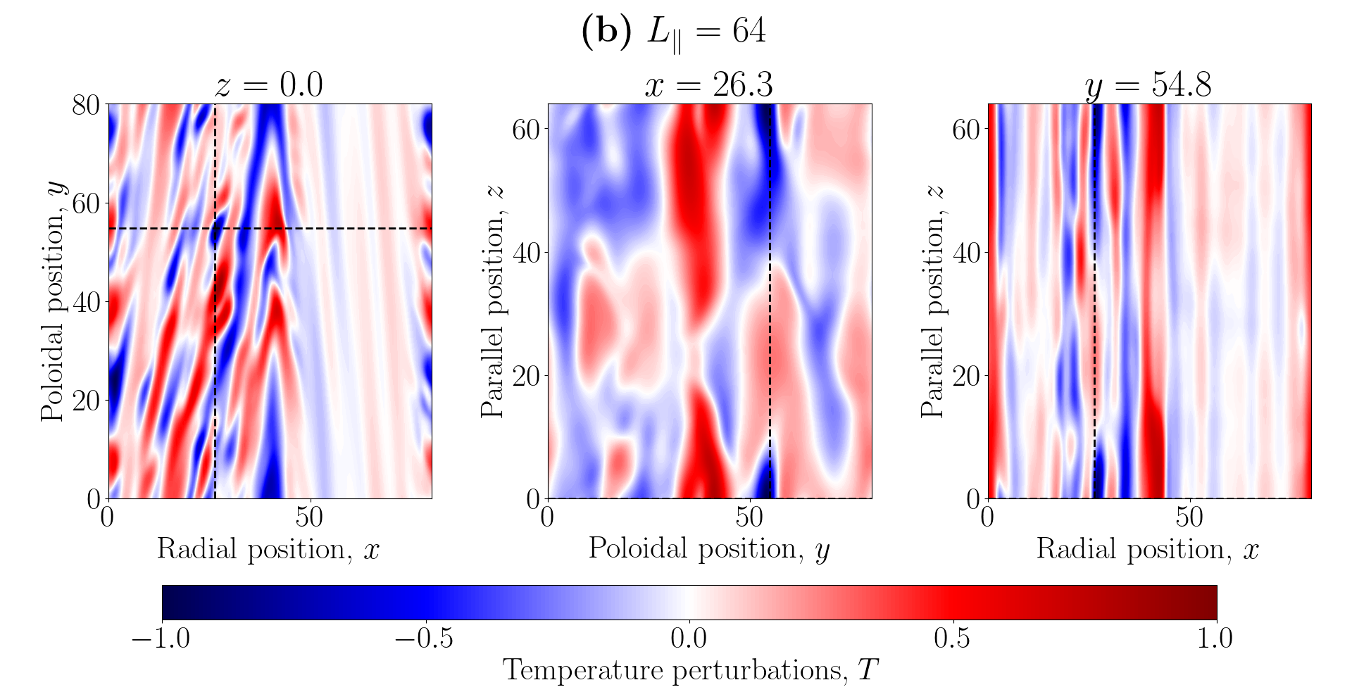
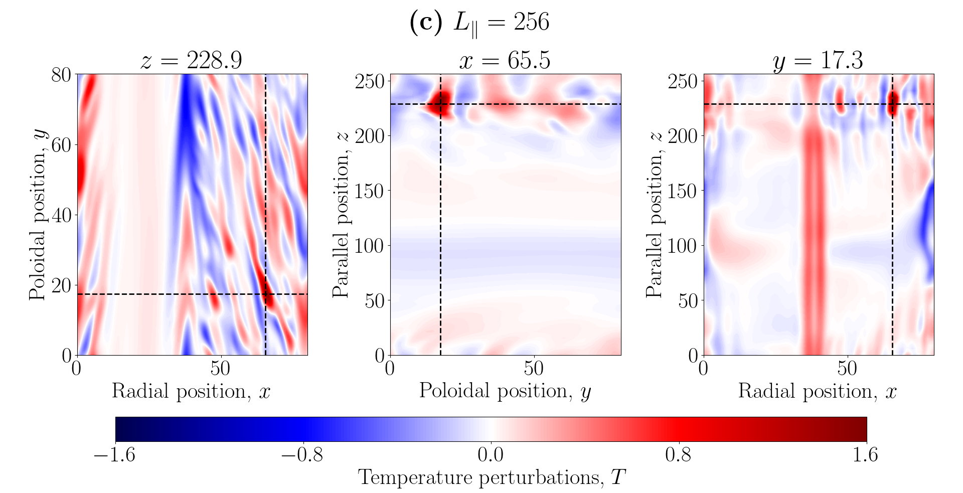
Figure 7: Snapshots of the 3D temperature perturbations associated with a ferdinon. The plots in each row are cross sections in different planes at the same $t$ taken from simulations that have the same $\kappa_{T}=0.36$, $\chi=0.1$, $L_{x}=L_{y}=80$, but (a) $L_{\parallel}=32$, (b) $L_{\parallel}=64$, and (c) $L_{\parallel}=256$. The black dashed lines visualise the intersections of the cross-sectional planes. As we increase $L_{\parallel}$, turbulence loses the ability to stay coherent along the parallel extent of the box and the bursts become localised in $z$.

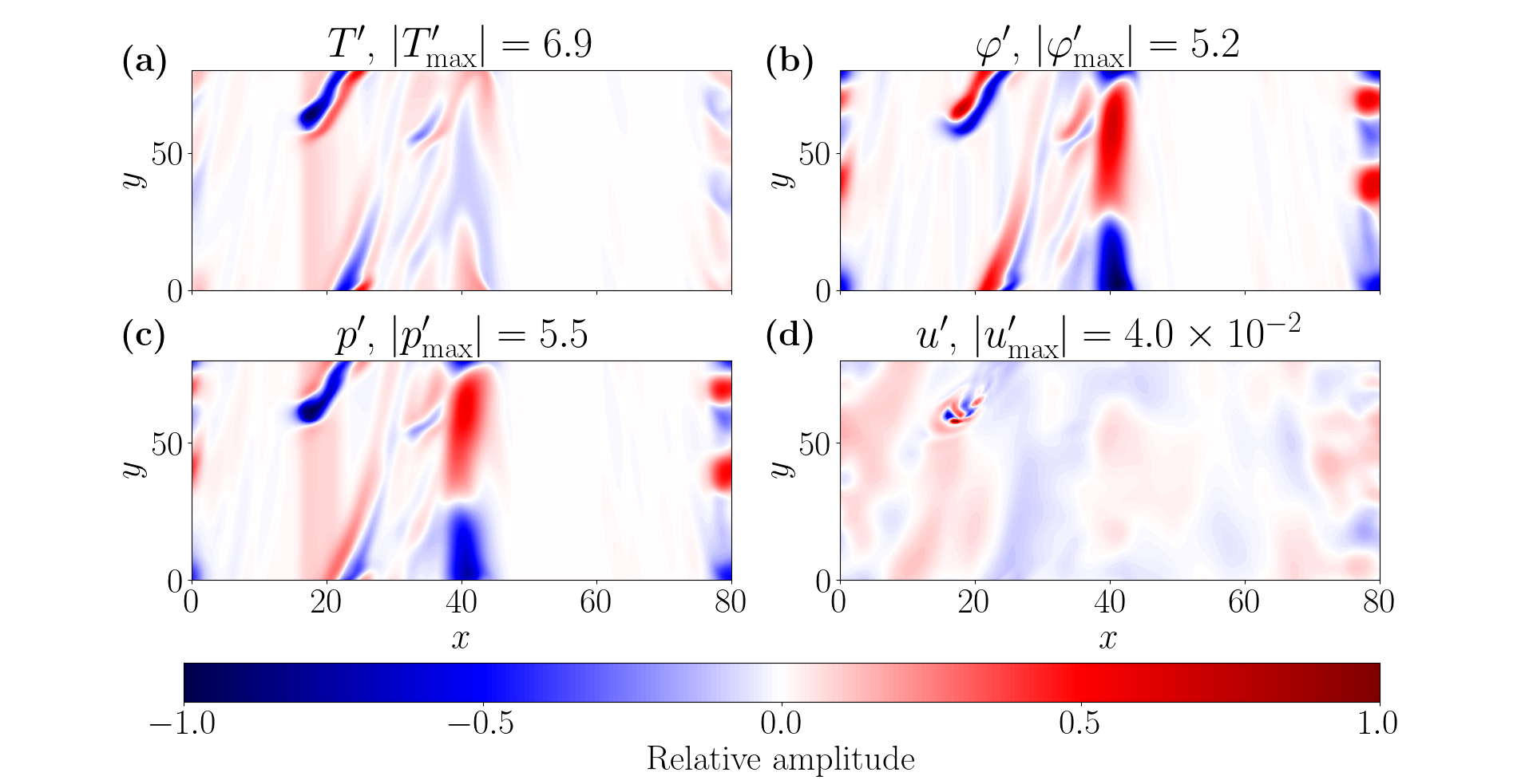
Figure 8: Snapshots of perturbed nonzonal (a) temperature, (b) potential, (c) pressure, and (d) parallel velocity at fixed $z$ in the Dimits state with parameters $\kappa_{T}=0.8$, $\chi=0.1$, $L_{x}=L_{y}=80$, $L_{\parallel}=1$, parallel hyperviscosity $\nu=2.4\times 10^{-8}$, and Fourier-space resolution $(n_{x},n_{y},n_{z})=(171,171,21)$. The colour scale is relative to the maximum absolute amplitude in each panel (given in the panel’s title). Small-scale sITG modes driven by the gradients of the ferdinon are evident in panel (d).

Secondly, we find small-scale sITG modes that feed off the perpendicular temperature gradients associated with the ferdinons. The presence of this three-dimensional small-scale ‘parasitic’ instability can be detected via the parallel velocity ${u}$, because the latter is only involved in the 3D sITG modes and not in the 2D cITG modes. Figure 8 shows an example of a ferdinon that is ‘infected’ with such small-scale sITG instabilities. As we shall discuss in section 4.2, the small-scale instability leads to an effective increase in thermal diffusion, and thus an increase in the effective damping at large scales that reduces the large-scale temperature perturbations. This additional damping likely contributes to the reduced $Q$ of the 3D Dimits state. It also enables saturation at finite amplitude when the Dimits state is broken (section 4.3).

4.2 The parasitic slab-ITG instability and its role in the saturated state

4.2.1 Numerical evidence

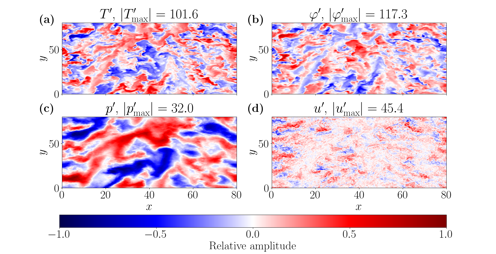
Figure 9: Snapshots of perturbed nonzonal (a) temperature, (b) potential, (c) pressure, and (d) parallel velocity at fixed $z$ in the strongly turbulent state with parameters $\kappa_{T}=3$, $\chi=0.05$, $L_{x}=L_{y}=80$, $L_{\parallel}=1$, parallel hyperviscosity $\nu=1.5\times 10^{-10}$, and Fourier-space resolution $(n_{x},n_{y},n_{z})=(285,285,83)$. The colour scale is relative to the maximum absolute amplitude in each panel (given in the panel’s title). Time-averaged spectra from the same simulation are shown in fig. 10.

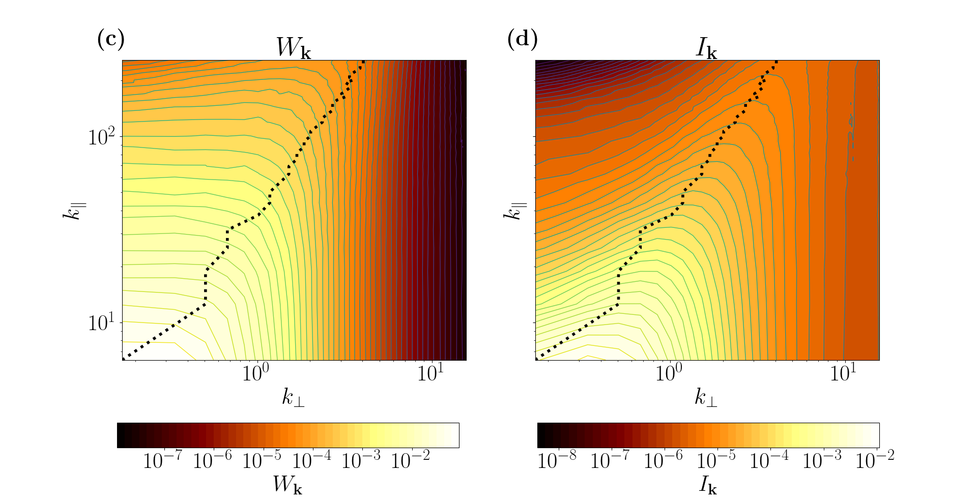
Figure 10: Time-averaged spectra (a) $W_{\boldsymbol{k}}$ and (b) $I_{\boldsymbol{k}}$, defined by eq. 17 and eq. 18, respectively, in the strongly turbulent state with parameters $\kappa_{T}=3$, $\chi=0.05$, $L_{x}=80$, $L_{y}=80$, and $L_{\parallel}=1$. The solid black lines demarcate the region of linear instability for $k_{x}=0$, and the red dashed line is $k_{\parallel}=\kappa_{T}k_{\perp}^{2}$, where the collisionless modes with largest growth rate reside (see section 3.3.2). We can see that the largest contributions to the two conserved quantities are offset from the region of linear instability. The dotted black line denotes the peak $k_{\perp,I}(k_{\parallel})$ of $I_{\boldsymbol{k}}$ at fixed $k_{\parallel}$. Zonal profiles and cross-sectional snapshots from the same simulation are shown in fig. 4 and fig. 9, respectively. The spectra of the saturated state with the same parameters, but with $\kappa_{T}$ set to $0$ for all $k_{\parallel}\neq 0$ modes, are given in (c) and (d). Turning off the equilibrium gradient for the 3D modes does not alter the spectra noticeably. Snapshots from this modified simulation are shown in fig. 11.

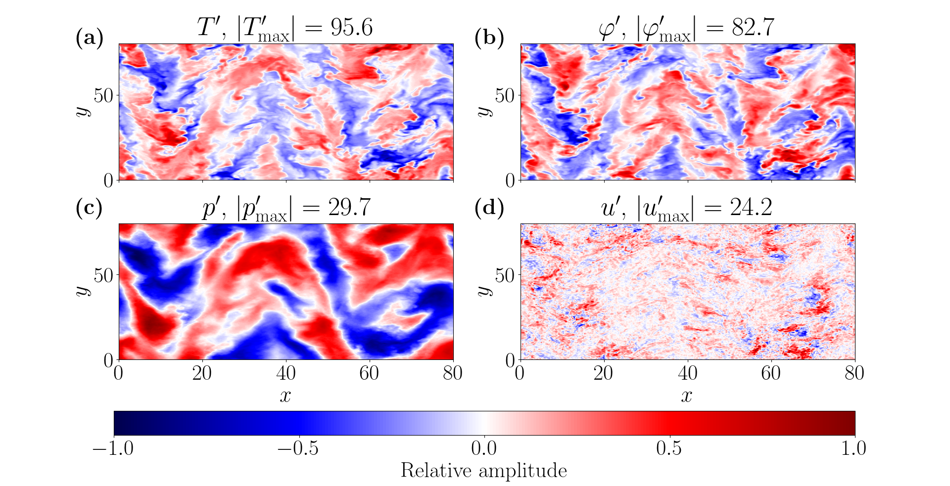
Figure 11: Same as fig. 9, but for a modified simulation, i.e., with $\kappa_{T}$ set to $0$ for the $k_{\parallel}\neq 0$ modes. Visually, the saturated state is identical to that shown in fig. 9.

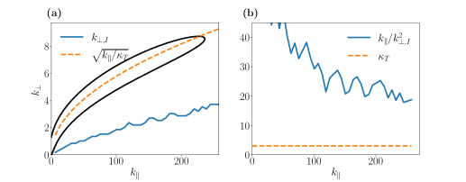
Figure 12: (a) Comparison of the location of the spectral peak $k_{\perp,I}(k_{\parallel})$ of $I_{\boldsymbol{k}}$ (blue line) and the location of the peak of the growth rate of the collisionless linear instability driven by the equilibrium gradient (orange dashed line), given by $k_{\parallel}=\kappa_{T}k_{\perp}^{2}$. The black curve circumscribes the region of linear instability, i.e., all ${\text{Im}{\mathopen{}\mathclose{{}\left(\omega_{\boldsymbol{k}}}\right)}}\geq 0$ solutions to eq. 20 are inside it and outside of it, all solutions satisfy ${\text{Im}{\mathopen{}\mathclose{{}\left(\omega_{\boldsymbol{k}}}\right)}}\leq 0$. (b) Comparison of the equilibrium temperature gradient $\kappa_{T}$ and the ‘effective’ temperature gradient $\kappa_{T}^{\text{eff}}(k_{\parallel})\equiv k_{\parallel}/k_{\perp,I}^{2}$. The data is from the same simulation as shown in fig. 9. The spectra of this simulation are given in fig. 10. This rough estimate of $\kappa_{T}^{\text{eff}}$ being about 5–10 times larger than $\kappa_{T}$ is consistent with the calculated growth rate of the parasitic small-scale instability (see fig. 13).

Let us now address the small-scale sITG instability. This instability exists only in the 3D model and is the most important distinction between it and its 2D counterpart. It is the presence of this instability that enables, in 3D and with finite $L_{\parallel}$, the existence of a strongly turbulent saturated state, i.e., one in which there are no strong, coherent ZFs (the zonal profiles of such a state are shown in figures 4d–f). We find that the most distinctive feature of this state is the concentration of pressure perturbations at perpendicular scales that are much larger than the typical (small) scales for the perturbations in $\varphi$ and $T$ (or, to be more precise, the absence of pressure perturbations in the small-scale structure present in $\varphi$ and $T$). This is manifest in fig. 9.

In section 3.3.2, we showed that the smallness of the pressure perturbations (compared to the perturbations of the electrostatic potential and temperature) was characteristic of the small-scale ($k_{\perp}\gg 1$) sITG instability: see (45). However, the small-scale structure that we see in fig. 9 is not produced by the equilibrium-driven instability. In fact, the equilibrium-driven sITG instability is inconsequential in the saturated state. To show this, we ran artificially modified simulations where $\kappa_{T}$ was set to $0$ for all modes with $k_{\parallel}\neq 0$ (this is straightforward to do in our spectral code). This removed the equilibrium-driven linear instability from all 3D ($k_{\parallel}\neq 0$) modes. Examining the spectra of the two conserved quantities $W_{\boldsymbol{k}}$ and $I_{\boldsymbol{k}}$ (see section 2.2), we see that turning off the equilibrium temperature gradient for the 3D modes has no noticeable effect on the structure of turbulence (see fig. 10). As fig. 11 shows, the modified simulations are also visually indistinguishable from the unmodified ones shown in fig. 9. The total heat flux $Q$ changes by about 20-30%, likely due to the loss of radial-symmetry breaking for the 3D modes, which are now free to transport heat in either direction equally, so on average, they have zero radial heat flux. The nonlinear interactions between the 2D ($k_{\parallel}=0$) modes cannot produce the 3D modes that we see in the modified simulations. Therefore, these 3D modes must be produced by a ‘parasitic’ sITG instability of the 2D fields (into which energy is injected by the equilibrium gradient).

Furthermore, the spectra of $W_{\boldsymbol{k}}$ and $I_{\boldsymbol{k}}$ measured in regular simulations are inconsistent with the region of linear instability of the dispersion relation eq. 20. Namely, figures 10a and 10b show that $W_{\boldsymbol{k}}$ and $I_{\boldsymbol{k}}$ of the linearly unstable modes of eq. 20 are orders of magnitude smaller than the corresponding spectral peaks of the two conserved quantities. We can quantify this by using the turbulent spectra to determine the ‘dominant’ perpendicular scale as a function of the parallel scale $k_{\parallel}$. As figures 10a and 10b show, this is the scale at which $I_{\boldsymbol{k}}$ peaks and the dependence of $W_{\boldsymbol{k}}$ on $k_{\perp}$ changes from flat to steeply declining. To extract this scale, we define $k_{\perp,I}(k_{\parallel})$ as the $k_{\perp}$ that maximises $I_{\boldsymbol{k}}$ at a fixed $k_{\parallel}$. Figure 12a shows that $k_{\perp,I}(k_{\parallel})$ lies outside of the region of linear instability of eq. 20. Thus, the 3D structure of the saturated state is not produced by the linear sITG instability driven by the equilibrium gradient.

In section 3.3.2, we showed that the equilibrium-driven sITG instability is localised at $k_{\parallel}\approx\kappa_{T}k_{\perp}^{2}$. A similar relationship holds for $k_{\perp,I}(k_{\parallel})$, viz., $k_{\parallel}\approx\kappa_{T}^{\text{eff}}k_{\perp,I}^{2}$, where $\kappa_{T}^{\text{eff}}$ can be thought of as an effective temperature gradient. Figure 12b shows that this $\kappa_{T}^{\text{eff}}$ is several times larger than the equilibrium temperature gradient. As we shall see shortly, $\kappa_{T}^{\text{eff}}$ is actually the gradient of the large-scale 2D temperature perturbations.

4.2.2 Scale-separated equations for curvature-ITG and slab-ITG modes

The numerical analysis above leads us to believe that the 3D structure of the saturated state is a consequence of an instability driven not by the equilibrium gradient $\kappa_{T}$, but rather by the gradients of the 2D perturbations. Let us attack on the analytical front. As we discussed at the start of section 4, the 3D sITG modes are naturally scale-separated from the 2D cITG modes both in wavenumber and in frequency. We then introduce the parallel average

$$\mathopen{}\mathclose{{}\left\langle f}\right\rangle_{\parallel}\equiv\int\frac{dz^{\prime}}{L_{z}}f(z^{\prime}).$$ (57)

This average allows us to split eq. 11–eq. 13 into separate equations for the slow 2D modes governed by the cITG instability at large perpendicular scales ($k_{\perp}\ll 1$), and for the fast 3D sITG modes, which live at small perpendicular scales ($k_{\perp}\gg 1$). We define the small-scale perturbations as $\widetilde{f}\equiv f-\mathopen{}\mathclose{{}\left\langle f}\right\rangle_{\parallel}$. The large-scale equations are then

$$\partial_{t}\mathopen{}\mathclose{{}\left(\mathopen{}\mathclose{{}\left\langle\varphi^{\prime}}\right\rangle_{\parallel}-\nabla_{\perp}^{2}\mathopen{}\mathclose{{}\left\langle\varphi}\right\rangle_{\parallel}}\right)-\partial_{y}\mathopen{}\mathclose{{}\left(\mathopen{}\mathclose{{}\left\langle\varphi}\right\rangle_{\parallel}+\mathopen{}\mathclose{{}\left\langle T}\right\rangle_{\parallel}}\right)+\kappa_{T}\partial_{y}\nabla_{\perp}^{2}\mathopen{}\mathclose{{}\left\langle\varphi}\right\rangle_{\parallel}$$

$$+\mathopen{}\mathclose{{}\left\{\mathopen{}\mathclose{{}\left\langle\varphi}\right\rangle_{\parallel},\mathopen{}\mathclose{{}\left\langle\varphi^{\prime}}\right\rangle_{\parallel}-\nabla_{\perp}^{2}\mathopen{}\mathclose{{}\left\langle\varphi}\right\rangle_{\parallel}}\right\}+{\boldsymbol{\nabla}}_{\perp}\bcdot\mathopen{}\mathclose{{}\left\{{\boldsymbol{\nabla}}_{\perp}\mathopen{}\mathclose{{}\left\langle\varphi}\right\rangle_{\parallel},\mathopen{}\mathclose{{}\left\langle T}\right\rangle_{\parallel}}\right\}+\chi\nabla_{\perp}^{4}\mathopen{}\mathclose{{}\left(a\mathopen{}\mathclose{{}\left\langle\varphi}\right\rangle_{\parallel}-b\mathopen{}\mathclose{{}\left\langle T}\right\rangle_{\parallel}}\right)=$$

$$-\mathopen{}\mathclose{{}\left\langle\mathopen{}\mathclose{{}\left\{\widetilde{\varphi},\widetilde{\varphi}^{\prime}-\nabla_{\perp}^{2}\widetilde{\varphi}}\right\}-{\boldsymbol{\nabla}}_{\perp}\bcdot\mathopen{}\mathclose{{}\left\{{\boldsymbol{\nabla}}_{\perp}\widetilde{\varphi},\widetilde{T}}\right\}}\right\rangle_{\parallel},$$ (58)

$$\partial_{t}\mathopen{}\mathclose{{}\left\langle T}\right\rangle_{\parallel}+\kappa_{T}\partial_{y}\mathopen{}\mathclose{{}\left\langle\varphi}\right\rangle_{\parallel}+\mathopen{}\mathclose{{}\left\{\mathopen{}\mathclose{{}\left\langle\varphi}\right\rangle_{\parallel},\mathopen{}\mathclose{{}\left\langle T}\right\rangle_{\parallel}}\right\}-\chi\nabla_{\perp}^{2}\mathopen{}\mathclose{{}\left\langle T}\right\rangle_{\parallel}=-\mathopen{}\mathclose{{}\left\langle\mathopen{}\mathclose{{}\left\{\widetilde{\varphi},\widetilde{T}}\right\}}\right\rangle_{\parallel},$$ (59)

$$\partial_{t}\mathopen{}\mathclose{{}\left\langle{u}}\right\rangle_{\parallel}+\mathopen{}\mathclose{{}\left\{\mathopen{}\mathclose{{}\left\langle\varphi}\right\rangle_{\parallel},\mathopen{}\mathclose{{}\left\langle{u}}\right\rangle_{\parallel}}\right\}-s\chi\nabla_{\perp}^{2}\mathopen{}\mathclose{{}\left\langle{u}}\right\rangle_{\parallel}=-\mathopen{}\mathclose{{}\left\langle\mathopen{}\mathclose{{}\left\{\widetilde{\varphi},\widetilde{{u}}}\right\}}\right\rangle_{\parallel}.$$ (60)

The right-hand sides of eq. 58–eq. 60 represent the influence of the 3D sITG modes on the large-scale fields. Subtracting eq. 58–eq. 60 from eq. 11–eq. 13, we find the small-scale equations:

$$\partial_{t}\mathopen{}\mathclose{{}\left(\widetilde{\varphi}^{\prime}-\nabla_{\perp}^{2}\widetilde{\varphi}}\right)+\partial_{\parallel}\widetilde{{u}}-\partial_{y}(\widetilde{\varphi}+\widetilde{T})+\kappa_{T}\partial_{y}\nabla_{\perp}^{2}\widetilde{\varphi}+\widetilde{\mathopen{}\mathclose{{}\left\{\widetilde{\varphi},\widetilde{\varphi}^{\prime}-\nabla_{\perp}^{2}\widetilde{\varphi}}\right\}}+{\boldsymbol{\nabla}}_{\perp}\bcdot\widetilde{\mathopen{}\mathclose{{}\left\{{\boldsymbol{\nabla}}_{\perp}\widetilde{\varphi},\widetilde{T}}\right\}}$$

$$+\chi\nabla_{\perp}^{4}\mathopen{}\mathclose{{}\left(a\widetilde{\varphi}-b\widetilde{T}}\right)=-\Big{[}\mathopen{}\mathclose{{}\left\{\mathopen{}\mathclose{{}\left\langle\varphi}\right\rangle_{\parallel},\widetilde{\varphi}^{\prime}-\nabla_{\perp}^{2}\widetilde{\varphi}}\right\}+\mathopen{}\mathclose{{}\left\{\widetilde{\varphi},\mathopen{}\mathclose{{}\left\langle\varphi^{\prime}}\right\rangle_{\parallel}-\nabla_{\perp}^{2}\mathopen{}\mathclose{{}\left\langle\varphi}\right\rangle_{\parallel}}\right\}$$

$$+{\boldsymbol{\nabla}}_{\perp}\bcdot\mathopen{}\mathclose{{}\left\{{\boldsymbol{\nabla}}_{\perp}\mathopen{}\mathclose{{}\left\langle\varphi}\right\rangle_{\parallel},\widetilde{T}}\right\}+{\boldsymbol{\nabla}}_{\perp}\bcdot\mathopen{}\mathclose{{}\left\{{\boldsymbol{\nabla}}_{\perp}\widetilde{\varphi},\mathopen{}\mathclose{{}\left\langle T}\right\rangle_{\parallel}}\right\}\Big{]},$$ (61)

$$\partial_{t}\widetilde{T}+\kappa_{T}\partial_{y}\widetilde{\varphi}+\widetilde{\mathopen{}\mathclose{{}\left\{\widetilde{\varphi},\widetilde{T}}\right\}}-\chi\nabla_{\perp}^{2}\widetilde{T}=-\mathopen{}\mathclose{{}\left[\mathopen{}\mathclose{{}\left\{\mathopen{}\mathclose{{}\left\langle\varphi}\right\rangle_{\parallel},\widetilde{T}}\right\}+\mathopen{}\mathclose{{}\left\{\widetilde{\varphi},\mathopen{}\mathclose{{}\left\langle T}\right\rangle_{\parallel}}\right\}}\right],$$ (62)

$$\partial_{t}\widetilde{{u}}+\partial_{\parallel}\mathopen{}\mathclose{{}\left(\widetilde{\varphi}+\widetilde{T}}\right)+\widetilde{\mathopen{}\mathclose{{}\left\{\widetilde{\varphi},\hat{u}}\right\}}-s\chi\nabla_{\perp}^{2}\hat{u}=-\mathopen{}\mathclose{{}\left[\mathopen{}\mathclose{{}\left\{\mathopen{}\mathclose{{}\left\langle\varphi}\right\rangle_{\parallel},\widetilde{{u}}}\right\}+\mathopen{}\mathclose{{}\left\{\widetilde{\varphi},\mathopen{}\mathclose{{}\left\langle{u}}\right\rangle_{\parallel}}\right\}}\right].$$ (63)

In order to simplify the following analysis, we shall assume both temporal and spatial scale separation between eq. 58–eq. 60 and eq. 61–eq. 63, i.e., that the large-scale fields are constant in time in eq. 61–eq. 63 and that the spatial and temporal scales of eq. 61–eq. 63 are short compared to the respective scales of eq. 58–eq. 60. In particular, we shall assume that the perpendicular scales of the 2D modes are sufficiently large for the derivatives of their gradients to be ignored. This assumption turns out to be equivalent to $k_{\perp}q_{\perp}\ll 1$, where $k_{\perp}$ and $q_{\perp}$ are the typical perpendicular wavenumbers of the 2D and parasitic modes, respectively. According to eq. 27 and eq. 52, the linearly unstable modes satisfy $k_{\perp}\sim\kappa_{T}^{-1/4}$ and $q_{\perp}\sim(\kappa_{T}/\chi)^{1/3}$ in the limit $\kappa_{T}\gg\chi$. Therefore, the condition $k_{\perp}q_{\perp}\ll 1$ is equivalent to $\chi\gg\kappa_{T}^{1/4}$. Additionally, recall that the Dimits threshold in 2D is found at $\kappa_{T}\sim\chi$ (Ivanov et al., 2020) and that, as we showed in section 4.1, the 2D Dimits regime is qualitatively unchanged when we include 3D effects. Thus, for the remainder of this section, we shall consider the limit

$$\kappa_{T}\gg\chi\gg\kappa_{T}^{1/4}\gg 1,$$ (64)

which puts us beyond the 2D Dimits transition (i.e., in 2D, such a state blows up). Importantly, we limit our analysis to $\kappa_{T}/\chi\ll 830$, in which case the $\chi$ITG instability can safely be neglected (see appendix C). The limit eq. 64 then allows us to simplify eq. 58–eq. 60 and eq. 61–eq. 63 significantly and thus to describe the interplay between 2D and parasitic modes analytically. These analytical results agree with our simulations, even though the latter do not strictly conform to eq. 64.

4.2.3 Parasitic slab-ITG instability

First, we investigate the small-scale sITG instability in the presence of large-scale 2D modes. Linearising eq. 61–eq. 63 in the limit eq. 64, we obtain

$$\mathopen{}\mathclose{{}\left(\partial_{t}+\mathopen{}\mathclose{{}\left\langle{\boldsymbol{V_{\text{{E}}}}}}\right\rangle_{\parallel}\bcdot{\boldsymbol{\nabla}}_{\perp}}\right)\mathopen{}\mathclose{{}\left(\widetilde{\varphi}^{\prime}-\nabla_{\perp}^{2}\widetilde{\varphi}}\right)+\partial_{\parallel}\widetilde{{u}}-\partial_{y}(\widetilde{\varphi}+\widetilde{T})$$

$$\quad+{\boldsymbol{\kappa}}_{T}\bcdot{\boldsymbol{\nabla}}_{\perp}\nabla_{\perp}^{2}\widetilde{\varphi}+{\boldsymbol{\kappa}}_{n}\bcdot{\boldsymbol{\nabla}}_{\perp}\widetilde{\varphi}=-\chi\nabla_{\perp}^{4}(a\widetilde{\varphi}-b\widetilde{T}),$$ (65)

$$\mathopen{}\mathclose{{}\left(\partial_{t}+\mathopen{}\mathclose{{}\left\langle{\boldsymbol{V_{\text{{E}}}}}}\right\rangle_{\parallel}\bcdot{\boldsymbol{\nabla}}_{\perp}}\right)\widetilde{T}+{\boldsymbol{\kappa}}_{T}\bcdot{\boldsymbol{\nabla}}_{\perp}\widetilde{\varphi}=\chi\nabla_{\perp}^{2}\widetilde{T},$$ (66)

$$\mathopen{}\mathclose{{}\left(\partial_{t}+\mathopen{}\mathclose{{}\left\langle{\boldsymbol{V_{\text{{E}}}}}}\right\rangle_{\parallel}\bcdot{\boldsymbol{\nabla}}_{\perp}}\right)\widetilde{{u}}+\partial_{\parallel}\mathopen{}\mathclose{{}\left(\widetilde{\varphi}+\widetilde{T}}\right)=s\nabla_{\perp}^{2}\widetilde{{u}},$$ (67)

where the ‘local-equilibrium’ quantities

$$\mathopen{}\mathclose{{}\left\langle{\boldsymbol{V_{\text{{E}}}}}}\right\rangle_{\parallel}\equiv\hat{{\boldsymbol{z}}}\times{\boldsymbol{\nabla}}_{\perp}\mathopen{}\mathclose{{}\left\langle\varphi}\right\rangle_{\parallel},\quad{\boldsymbol{\kappa}}_{n}\equiv-\hat{{\boldsymbol{z}}}\times{\boldsymbol{\nabla}}_{\perp}\mathopen{}\mathclose{{}\left\langle\varphi^{\prime}}\right\rangle_{\parallel},\quad{\boldsymbol{\kappa}}_{T}\equiv\kappa_{T}\hat{{\boldsymbol{y}}}-\hat{{\boldsymbol{z}}}\times{\boldsymbol{\nabla}}_{\perp}\mathopen{}\mathclose{{}\left\langle T}\right\rangle_{\parallel}$$ (68)

are the ${\boldsymbol{E}}\times{\boldsymbol{B}}$ advecting flow, the local density gradient, and the total local temperature gradient (large-scale perturbation plus equilibrium), respectively. We assume that $|{\boldsymbol{\kappa}}_{T}|\sim|{\boldsymbol{\kappa}}_{n}|$ (see section 4.2.4). Note that only the nonzonal electrostatic potential $\varphi^{\prime}$ gives rise to a density perturbation — this is a consequence of the modified adiabatic electron response eq. 1. Note also that we have ignored the large-scale 2D parallel flow $\mathopen{}\mathclose{{}\left\langle{u}}\right\rangle_{\parallel}$. Since $\mathopen{}\mathclose{{}\left\langle{u}}\right\rangle_{\parallel}$ is not involved in any linear instability, the only way it could be driven is via the small-scale response, viz., the right-hand side of eq. 60. In appendix E, we show that a small initial $\mathopen{}\mathclose{{}\left\langle{u}}\right\rangle_{\parallel}$ will decay under the influence of growing small-scale modes. Accordingly, in our numerical simulations, we find that $\mathopen{}\mathclose{{}\left\langle u}\right\rangle_{\parallel}$ is many orders of magnitude smaller than the other two 2D fields and is irrelevant for the saturated state.

Ignoring collisions (i.e., setting $\chi=0$) and taking the gradients of the large-scale fields to be constant over the small scales at which eq. 65–eq. 67 hold, we can investigate the small-scale linear instability in a way analogous to what we did in section 3. In particular, we shall focus on the $k_{\parallel}\sim k_{\perp}^{2}\gg 1$ regime analysed in section 3.3.2. We look for Doppler-shifted solutions to eq. 65–eq. 67 of the form $\widetilde{\varphi}_{\boldsymbol{k}},\widetilde{T}_{\boldsymbol{k}},\widetilde{{u}}_{\boldsymbol{k}}\propto\exp{[-i(\omega_{\boldsymbol{k}}+\mathopen{}\mathclose{{}\left\langle{\boldsymbol{V_{\text{{E}}}}}}\right\rangle_{\parallel}\bcdot{\boldsymbol{k}})t+i{\boldsymbol{k}}\bcdot{\boldsymbol{r}}]}$. Note that we ignore the shear in the ${\boldsymbol{E}}\times{\boldsymbol{B}}$ flow $\mathopen{}\mathclose{{}\left\langle{\boldsymbol{V_{\text{{E}}}}}}\right\rangle_{\parallel}$. We also ignore the magnetic-drift term $-\partial_{y}(\widetilde{\varphi}+\widetilde{T})$ in eq. 65 because it is subdominant for the sITG modes with $k_{\perp}\gg 1$. The resulting dispersion relation for these modes is

$$\mathopen{}\mathclose{{}\left(\omega_{\boldsymbol{k}}^{2}-\frac{k_{\parallel}^{2}}{1+k_{\perp}^{2}}}\right)\mathopen{}\mathclose{{}\left(\omega_{\boldsymbol{k}}+{\boldsymbol{\kappa}}_{T}\bcdot{\boldsymbol{k}}}\right)=\frac{\omega_{\boldsymbol{k}}^{2}}{1+k_{\perp}^{2}}\mathopen{}\mathclose{{}\left[\mathopen{}\mathclose{{}\left({\boldsymbol{\kappa}}_{n}+{\boldsymbol{\kappa}}_{T}}\right)\bcdot{\boldsymbol{k}}}\right].$$ (69)

Since eq. 65–eq. 67 describe real fields, eq. 69 must be invariant under ${\boldsymbol{k}}\mapsto-{\boldsymbol{k}}$ and $\omega_{\boldsymbol{k}}\mapsto-\omega_{\boldsymbol{k}}^{*}$. We may, therefore, assume that ${\boldsymbol{\kappa}}_{T}\bcdot{\boldsymbol{k}}>0$ without loss of generality. Repeating the arguments of section 3.3.2, we define $\omega_{\boldsymbol{k}}\equiv\hat{\omega}_{\boldsymbol{k}}{\boldsymbol{\kappa}}_{T}\bcdot{\boldsymbol{k}}$ and $k_{\parallel}\equiv\hat{k}_{\parallel}{\boldsymbol{\kappa}}_{T}\bcdot{\boldsymbol{k}}$. Then eq. 69 turns out to be formally the same as our old dispersion relation (31), but now with

$$\hat{\gamma}_{\boldsymbol{k}}^{2}=\frac{({\boldsymbol{\kappa}}_{n}+{\boldsymbol{\kappa}}_{T})\bcdot{\boldsymbol{k}}}{2k_{\perp}^{2}{\boldsymbol{\kappa}}_{T}\bcdot{\boldsymbol{k}}}.$$ (70)

Thus, the results of section 3.3.2 carry over to the parasitic instability described by eq. 69. In particular, the sITG instability exists if $\hat{\gamma}_{\boldsymbol{k}}^{2}>0$, i.e., if $({\boldsymbol{\kappa}}_{n}+{\boldsymbol{\kappa}}_{T})\bcdot{\boldsymbol{k}}$ and ${\boldsymbol{\kappa}}_{T}\bcdot{\boldsymbol{k}}$ have the same sign, and is localised to $k_{\parallel}\approx\pm{\boldsymbol{\kappa}}_{T}\bcdot{\boldsymbol{k}}k_{\perp}$. Its growth rate is given by

$${\text{Im}{\mathopen{}\mathclose{{}\left(\omega_{\boldsymbol{k}}}\right)}}\approx\text{Re}\sqrt{\frac{{\boldsymbol{\kappa}}_{T}\bcdot\hat{{\boldsymbol{k}}}\mathopen{}\mathclose{{}\left({\boldsymbol{\kappa}}_{n}+{\boldsymbol{\kappa}}_{T}}\right)\bcdot\hat{{\boldsymbol{k}}}}{2}},$$ (71)

where $\hat{{\boldsymbol{k}}}={\boldsymbol{k}}/k_{\perp}$. As expected, this is the same as eq. 44 if ${\boldsymbol{\kappa}}_{n}=0$ and ${\boldsymbol{\kappa}}_{T}=\kappa_{T}\hat{{\boldsymbol{y}}}$. In fig. 13b, we show the maximum growth rate obtained from the numerical solution of the full (with collisionality and magnetic curvature turned back on) dispersion relation eq. 20 with the addition of the local temperature and density gradients of the large-scale fields. As expected from the numerical analysis in section 4.2.1, the small-scale instability driven by the large-scale gradients is significantly ($\approx 5$ times in this case) stronger than the equilibrium-driven instability. This is consistent with the estimate of the effective temperature gradient $\kappa_{T}^{\text{eff}}$ for the sITG instability that we showed in fig. 12b.

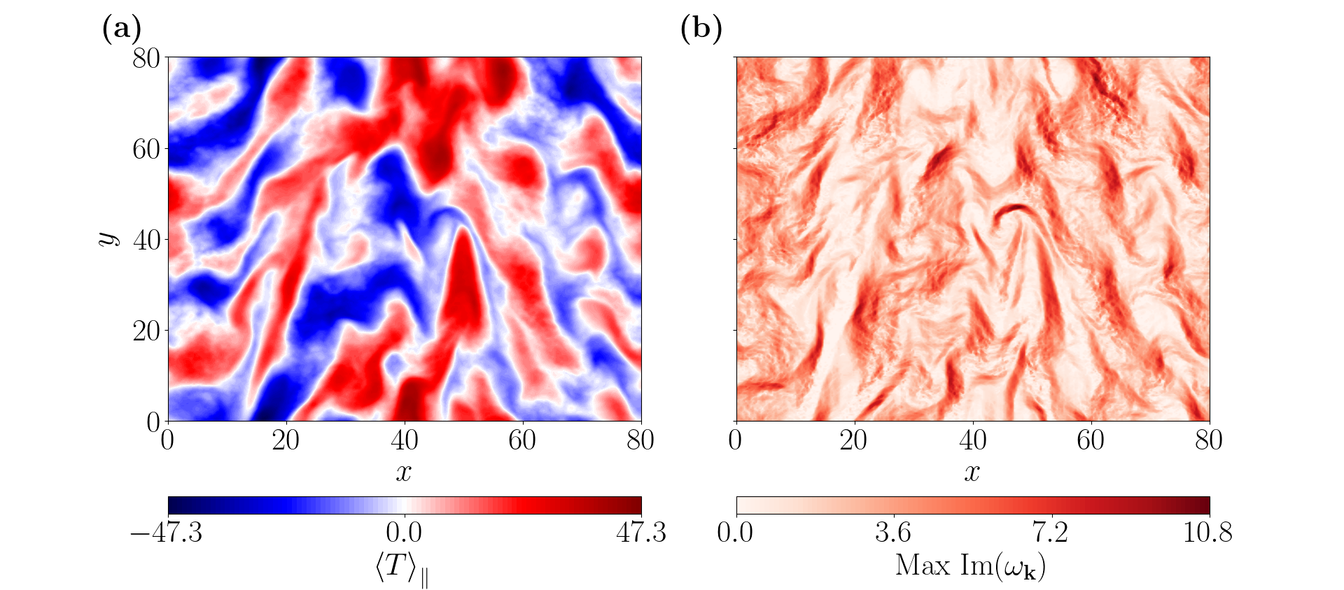
Figure 13: (a) Snapshot of the 2D temperature perturbation $\mathopen{}\mathclose{{}\left\langle T}\right\rangle_{\parallel}$ in the $(x,y)$ plane. The data is taken from the same $\kappa_{T}=3$, $\chi=0.05$ simulation that we showed in fig. 9. The 2D temperature perturbations lack the small-scale structure that was seen in fig. 9a, confirming that the parallel average eq. 57 removes small-scale perpendicular structure. (b) Small-scale growth rate in the $(x,y)$ plane. This plot is obtained by finding the maximum growth rate of the full (including collisionality and magnetic curvature) dispersion relation eq. 20 with the addition of the local temperature and density gradients of the large-scale fields at every point. For this simulation, $\kappa_{T}=3$, and so the largest collisionless growth rate, given by eq. 44, is $\kappa_{T}/\sqrt{2}\approx 2.1$. It is thus evident that the influence of the gradients of the large-scale fields dominates over that of the equilibrium gradient $\kappa_{T}$ by a factor of $5$. The ‘effective’ $\kappa_{T}^{\text{eff}}$ that we estimated for the same simulation in fig. 12b is, indeed, a factor of 5–10 larger that the equilibrium gradient $\kappa_{T}$.

Note that if ${\boldsymbol{\kappa}}_{n}\neq 0$, eq. 71 implies that modes with ${\boldsymbol{\kappa}}_{T}\bcdot{\boldsymbol{k}}\mathopen{}\mathclose{{}\left({\boldsymbol{\kappa}}_{n}+{\boldsymbol{\kappa}}_{T}}\right)\bcdot{\boldsymbol{k}}<0$ are linearly stable. Is there a ${\boldsymbol{\kappa}}_{n}$ that quenches the sITG instability for all ${\boldsymbol{k}}$? Suppose ${\boldsymbol{\kappa}}_{n}\nparallel{\boldsymbol{\kappa}}_{T}$. Then we can choose $\hat{{\boldsymbol{k}}}\bcdot{\boldsymbol{\kappa}}_{n}=0$, but $\hat{{\boldsymbol{k}}}\bcdot{\boldsymbol{\kappa}}_{T}\neq 0$. By eq. 71, any such $\hat{{\boldsymbol{k}}}$ is an unstable mode. Therefore, to stabilise all modes, we require ${\boldsymbol{\kappa}}_{n}\parallel{\boldsymbol{\kappa}}_{T}$. In this case, it is evident that ${\boldsymbol{\kappa}}_{n}\bcdot\hat{{\boldsymbol{k}}}=({\boldsymbol{\kappa}}_{n}\bcdot{\boldsymbol{\kappa}}_{T})({\boldsymbol{\kappa}}_{T}\bcdot\hat{{\boldsymbol{k}}})/|{\boldsymbol{\kappa}}_{T}|^{2}$. Therefore, in order to quench the sITG instability for all ${\boldsymbol{k}}$, we need

$${\boldsymbol{\kappa}}_{n}\parallel{\boldsymbol{\kappa}}_{T},\quad\frac{{\boldsymbol{\kappa}}_{n}\bcdot{\boldsymbol{\kappa}}_{T}}{|{\boldsymbol{\kappa}}_{T}|^{2}}\leq-1.$$ (72)

We shall now show that the effect of the growing small-scale modes on the large-scale 2D fields can be expressed as an enhanced thermal diffusivity for the latter.

4.2.4 Anomalous heat flux due to parasitic slab-ITG modes

We expect that the growth of small-scale sITG modes, which are driven by the gradients associated with the large-scale fluctuations, will check the growth of the amplitudes of the driving large-scale fields. This is an intuitive consequence of the conservation laws eq. 14 and section 2.2. As the parasitic instability is driven by the nonlinear terms that conserve $W=\sum_{\boldsymbol{k}}W_{\boldsymbol{k}}$ and $I=\sum_{\boldsymbol{k}}I_{\boldsymbol{k}}$, an excitation of parasitic small-scale modes should show up as a sink in the large-scale equations. Let us now calculate explicitly the influence of small-scale sITG modes on the large-scale modes and show that this is indeed true. This influence is represented by the terms of the form $\mathopen{}\mathclose{{}\left\langle\mathopen{}\mathclose{{}\left\{.,.}\right\}}\right\rangle_{\parallel}$ on the right-hand sides of eq. 58–eq. 60.

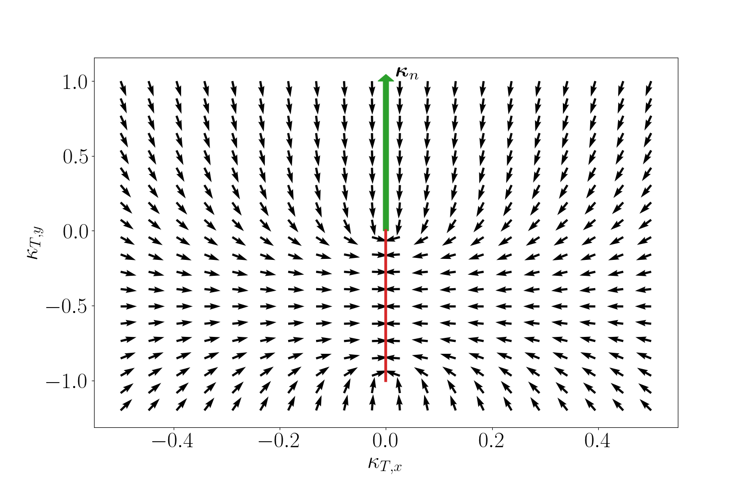
Figure 14: This plot shows the direction in which the heat flux eq. 74 of the most unstable small-scale mode ($\hat{{\boldsymbol{q}}}=\hat{{\boldsymbol{q}}}_{\text{max}}$) pushes the temperature gradient ${\boldsymbol{\kappa}}_{T}=-\hat{{\boldsymbol{z}}}\times{\boldsymbol{\nabla}}_{\perp}\mathopen{}\mathclose{{}\left\langle T}\right\rangle_{\parallel}$. We have chosen a coordinate system in which the large-scale density gradient is ${\boldsymbol{\kappa}}_{n}=(0,1)$, denoted by the green arrow. The red line shows the values of ${\boldsymbol{\kappa}}_{T}$ for which the sITG instability has zero growth rate, according to eq. 72. The black arrows represent the direction of $-\hat{{\boldsymbol{z}}}\times\langle\widetilde{{\boldsymbol{Q}}}\rangle_{\parallel}$. We see that $\langle\widetilde{{\boldsymbol{Q}}}\rangle_{\parallel}$ pushes the large-scale temperature gradient ${\boldsymbol{\kappa}}_{T}$ towards the linearly stable region.

First, consider the temperature equation eq. 59. The relevant term is

$$-\mathopen{}\mathclose{{}\left\langle\mathopen{}\mathclose{{}\left\{\widetilde{\varphi},\widetilde{T}}\right\}}\right\rangle_{\parallel}=-{\boldsymbol{\nabla}}_{\perp}\bcdot\mathopen{}\mathclose{{}\left\langle\mathopen{}\mathclose{{}\left[(\hat{{\boldsymbol{z}}}\times{\boldsymbol{\nabla}}_{\perp}\widetilde{\varphi})\widetilde{T}}\right]}\right\rangle_{\parallel}\equiv-{\boldsymbol{\nabla}}_{\perp}\bcdot\langle\widetilde{{\boldsymbol{Q}}}\rangle_{\parallel},$$ (73)

where $\langle\widetilde{{\boldsymbol{Q}}}\rangle_{\parallel}$ is the turbulent heat flux associated with the small-scale modes. Let us compute it quasilinearly (i.e., assuming that $\langle\widetilde{{\boldsymbol{Q}}}\rangle_{\parallel}$ is determined by the most unstable small-scale modes), assuming scale separation. As stated in section 4.2.2, we imagine that the small-scale equations are solved in an infinitesimal (compared to the large scales) box, and thus the parallel average is equivalent to an average over such a small-scale box:

$$\langle\widetilde{{\boldsymbol{Q}}}\rangle_{\parallel}=-\sum_{\boldsymbol{q}}i\hat{{\boldsymbol{z}}}\times{\boldsymbol{q}}\widetilde{\varphi}_{-{\boldsymbol{q}}}\widetilde{T}_{\boldsymbol{q}}\approx-\sum_{\boldsymbol{q}}\hat{{\boldsymbol{z}}}\times\hat{{\boldsymbol{q}}}\sqrt{\frac{({\boldsymbol{\kappa}}_{T}+{\boldsymbol{\kappa}}_{n})\bcdot\hat{{\boldsymbol{q}}}}{2{\boldsymbol{\kappa}}_{T}\bcdot\hat{{\boldsymbol{q}}}}}|\widetilde{\varphi}_{\boldsymbol{q}}|^{2},$$ (74)

where $\hat{{\boldsymbol{q}}}={\boldsymbol{q}}/q_{\perp}$ and we have assumed that the sum is dominated by the wavenumbers ${\boldsymbol{q}}$ corresponding to the largest linear growth rate of the parasitic sITG instability, and so have replaced $\widetilde{T}_{\boldsymbol{q}}/\widetilde{\varphi}_{\boldsymbol{q}}$ with the collisionless expression eq. 45 for the modes with $k_{\parallel}={\boldsymbol{\kappa}}_{T}\bcdot{\boldsymbol{k}}k_{\perp}$ that maximise this growth rate. Note that the small-scale fields $\widetilde{T}_{\boldsymbol{q}}$ and $\widetilde{\varphi}_{\boldsymbol{q}}$, and thus $\langle\widetilde{{\boldsymbol{Q}}}\rangle_{\parallel}$ itself, depend implicitly on the position variable of the large-scale equations eq. 58–eq. 60.

In order to verify that $\langle\widetilde{{\boldsymbol{Q}}}\rangle_{\parallel}$ does indeed damp the large-scale temperature perturbations $\mathopen{}\mathclose{{}\left\langle T}\right\rangle_{\parallel}$, we multiply eq. 59 by $\mathopen{}\mathclose{{}\left\langle T}\right\rangle_{\parallel}$ and integrate over space to find

$$\partial_{t}\int d^{3}{\boldsymbol{r}}\frac{1}{2}\mathopen{}\mathclose{{}\left\langle T}\right\rangle_{\parallel}^{2}+\text{linear terms}=\int d^{3}{\boldsymbol{r}}\langle\widetilde{{\boldsymbol{Q}}}\rangle_{\parallel}\bcdot{\boldsymbol{\nabla}}_{\perp}\mathopen{}\mathclose{{}\left\langle T}\right\rangle_{\parallel}$$

$$\approx-\int d^{3}{\boldsymbol{r}}\sum_{\boldsymbol{q}}(\hat{{\boldsymbol{z}}}\times\hat{{\boldsymbol{q}}})\bcdot{\boldsymbol{\nabla}}_{\perp}\mathopen{}\mathclose{{}\left\langle T}\right\rangle_{\parallel}\sqrt{\frac{({\boldsymbol{\kappa}}_{T}+{\boldsymbol{\kappa}}_{n})\bcdot\hat{{\boldsymbol{q}}}}{2{\boldsymbol{\kappa}}_{T}\bcdot\hat{{\boldsymbol{q}}}}}|\widetilde{\varphi}_{\boldsymbol{q}}|^{2}$$

$$=-\int d^{3}{\boldsymbol{r}}\sum_{\boldsymbol{q}}\sqrt{\frac{{\boldsymbol{\kappa}}_{T}\bcdot\hat{{\boldsymbol{q}}}({\boldsymbol{\kappa}}_{T}+{\boldsymbol{\kappa}}_{n})\bcdot\hat{{\boldsymbol{q}}}}{2}}|\widetilde{\varphi}_{\boldsymbol{q}}|^{2}=-\int d^{3}{\boldsymbol{r}}\sum_{\boldsymbol{q}}{\text{Im}{\mathopen{}\mathclose{{}\left(\omega_{\boldsymbol{k}}}\right)}}|\widetilde{\varphi}_{\boldsymbol{q}}|^{2},$$ (75)

where ${\text{Im}{\mathopen{}\mathclose{{}\left(\omega_{\boldsymbol{k}}}\right)}}$ is the sITG growth rate eq. 71. Thus, the linearly unstable small-scale modes have a sign-definite effect on $\mathopen{}\mathclose{{}\left\langle T}\right\rangle_{\parallel}$: they provide additional dissipation.

The heat flux eq. 74 depends on $\mathopen{}\mathclose{{}\left\langle T}\right\rangle_{\parallel}$ in a nontrivial way. Let us quantify its influence on $\mathopen{}\mathclose{{}\left\langle T}\right\rangle_{\parallel}$ by working out its direction as a function of ${\boldsymbol{\kappa}}_{T}$. Let us assume that $\langle\widetilde{{\boldsymbol{Q}}}\rangle_{\parallel}$ is dominated by the fastest-growing sITG modes, and let their wavevector direction be $\hat{{\boldsymbol{q}}}_{\text{max}}$, so $\langle\widetilde{{\boldsymbol{Q}}}\rangle_{\parallel}$ is parallel to $\hat{{\boldsymbol{z}}}\times\hat{{\boldsymbol{q}}}_{\text{max}}$. In fig. 14, we illustrate the influence on ${\boldsymbol{\kappa}}_{T}$ of the contribution to $\langle\widetilde{{\boldsymbol{Q}}}\rangle_{\parallel}$ from the most unstable small-scale modes. As expected, we find that the turbulent heat flux due to the small-scale modes pushes the large-scale gradient ${\boldsymbol{\kappa}}_{T}$ towards the linearly stable configuration eq. 72.

Now consider eq. 58, the evolution equation for $\mathopen{}\mathclose{{}\left\langle\varphi}\right\rangle_{\parallel}$. The relevant nonlinear terms are

$$\mathopen{}\mathclose{{}\left\langle\mathopen{}\mathclose{{}\left\{\widetilde{\varphi},\widetilde{\varphi}^{\prime}-\nabla_{\perp}^{2}\widetilde{\varphi}}\right\}+{\boldsymbol{\nabla}}_{\perp}\bcdot\mathopen{}\mathclose{{}\left\{{\boldsymbol{\nabla}}_{\perp}\widetilde{\varphi},\widetilde{T}}\right\}}\right\rangle_{\parallel}={\boldsymbol{\nabla}}_{\perp}\bcdot\mathopen{}\mathclose{{}\left\langle\mathopen{}\mathclose{{}\left\{{\boldsymbol{\nabla}}_{\perp}\widetilde{\varphi},\widetilde{p}}\right\}}\right\rangle_{\parallel}$$

$$\quad={\boldsymbol{\nabla}}_{\perp}{\boldsymbol{\nabla}}_{\perp}\mathbf{:}\sum_{\boldsymbol{q}}(\hat{{\boldsymbol{z}}}\times{\boldsymbol{q}}){\boldsymbol{q}}\mathopen{}\mathclose{{}\left(1+{\text{Re}{\frac{\widetilde{T}_{\boldsymbol{q}}}{\widetilde{\varphi}_{\boldsymbol{q}}}}}}\right)|\widetilde{\varphi}_{\boldsymbol{q}}|^{2}\equiv{\boldsymbol{\nabla}}_{\perp}{\boldsymbol{\nabla}}_{\perp}\mathbf{:}\langle\widetilde{\Uppi}\rangle_{\parallel}.$$ (76)

The collisionless calculations of section 3.3.2 are straightforward to generalise for the collisionless parasitic small-scale instability. They yield the same relation for ${\text{Re}{(\widetilde{T}_{\boldsymbol{q}}/\widetilde{\varphi}_{\boldsymbol{q}})}}$, viz., $1+{\text{Re}{(\widetilde{T}_{\boldsymbol{q}}/\widetilde{\varphi}_{\boldsymbol{q}})}}=\mathcal{O}(q_{\perp}^{-2})$. However, as we shall discuss in section 4.2.5, the presence of nonzero $\chi$ alters this to $1+{\text{Re}{(\widetilde{T}_{\boldsymbol{q}}/\widetilde{\varphi}_{\boldsymbol{q}})}}=\mathcal{O}(q_{\perp}^{-1})$. Assuming therefore that the dominant parasitic modes satisfy $1+{\text{Re}{(\widetilde{T}_{\boldsymbol{q}}/\widetilde{\varphi}_{\boldsymbol{q}})}}\lesssim\mathcal{O}(q_{\perp}^{-1})$, we find ${\boldsymbol{\nabla}}_{\perp}{\boldsymbol{\nabla}}_{\perp}\mathbf{:}\langle\widetilde{\Uppi}\rangle_{\parallel}\lesssim k_{\perp}^{2}q_{\perp}|\hat{\varphi}|^{2}$. However, eq. 74 implies ${\boldsymbol{\nabla}}_{\perp}\bcdot\langle\widetilde{{\boldsymbol{Q}}}\rangle_{\parallel}\sim k_{\perp}|\hat{\varphi}|^{2}$, and so

$$\frac{{\boldsymbol{\nabla}}_{\perp}{\boldsymbol{\nabla}}_{\perp}\mathbf{:}\langle\widetilde{\Uppi}\rangle_{\parallel}}{{\boldsymbol{\nabla}}_{\perp}\bcdot\langle\widetilde{{\boldsymbol{Q}}}\rangle_{\parallel}}\lesssim k_{\perp}q_{\perp}\sim\mathcal{O}\mathopen{}\mathclose{{}\left[\mathopen{}\mathclose{{}\left(\frac{\kappa_{T}^{1/4}}{\chi}}\right)^{1/3}}\right]\ll 1,$$ (77)

in line with the assumption on scales formulated at the end of section 4.2.2. Therefore, assuming that $\mathopen{}\mathclose{{}\left\langle\varphi^{\prime}}\right\rangle_{\parallel}\sim\mathopen{}\mathclose{{}\left\langle T}\right\rangle_{\parallel}$ and that they evolve on the same time scale, we conclude that the main effect of the small-scale modes is to provide a feedback to the large-scale temperature in the form of the additional heat flux $\langle\widetilde{{\boldsymbol{Q}}}\rangle_{\parallel}$.

We can thus summarise the equations that govern the evolution of $\mathopen{}\mathclose{{}\left\langle\varphi^{\prime}}\right\rangle_{\parallel}$ and $\mathopen{}\mathclose{{}\left\langle T}\right\rangle_{\parallel}$ as

$$\partial_{t}\mathopen{}\mathclose{{}\left\langle\varphi^{\prime}}\right\rangle_{\parallel}-\partial_{y}\mathopen{}\mathclose{{}\left(\mathopen{}\mathclose{{}\left\langle\varphi^{\prime}}\right\rangle_{\parallel}+\mathopen{}\mathclose{{}\left\langle T^{\prime}}\right\rangle_{\parallel}}\right)+\kappa_{T}\partial_{y}\nabla_{\perp}^{2}\mathopen{}\mathclose{{}\left\langle\varphi^{\prime}}\right\rangle_{\parallel}$$

$$+\mathopen{}\mathclose{{}\left\{\mathopen{}\mathclose{{}\left\langle\varphi}\right\rangle_{\parallel},\mathopen{}\mathclose{{}\left\langle\varphi^{\prime}}\right\rangle_{\parallel}-\nabla_{\perp}^{2}\mathopen{}\mathclose{{}\left\langle\varphi}\right\rangle_{\parallel}}\right\}^{\prime}+{\boldsymbol{\nabla}}_{\perp}\bcdot\mathopen{}\mathclose{{}\left\{{\boldsymbol{\nabla}}_{\perp}\mathopen{}\mathclose{{}\left\langle\varphi}\right\rangle_{\parallel},\mathopen{}\mathclose{{}\left\langle T}\right\rangle_{\parallel}}\right\}^{\prime}+\chi\nabla_{\perp}^{4}\mathopen{}\mathclose{{}\left(a\mathopen{}\mathclose{{}\left\langle\varphi^{\prime}}\right\rangle_{\parallel}-b\mathopen{}\mathclose{{}\left\langle T^{\prime}}\right\rangle_{\parallel}}\right)=0$$ (78)

$$\partial_{t}\mathopen{}\mathclose{{}\left\langle T}\right\rangle_{\parallel}+\kappa_{T}\partial_{y}\mathopen{}\mathclose{{}\left\langle\varphi}\right\rangle_{\parallel}+\mathopen{}\mathclose{{}\left\{\mathopen{}\mathclose{{}\left\langle\varphi}\right\rangle_{\parallel},\mathopen{}\mathclose{{}\left\langle T}\right\rangle_{\parallel}}\right\}-\chi\nabla_{\perp}^{2}\mathopen{}\mathclose{{}\left\langle T}\right\rangle_{\parallel}=-\mathopen{}\mathclose{{}\left\langle\mathopen{}\mathclose{{}\left\{\widetilde{\varphi},\widetilde{T}}\right\}}\right\rangle_{\parallel},$$ (79)

where the influence of small-scale fields appears only in the temperature equation eq. 79. The system of eq. 65–eq. 67 and eq. 78–eq. 79 respects the conservation of the two conserved quantities described in section 2.2 — this is shown in appendix F.

The above reasoning does not apply to the ZFs. Indeed, the equation for $\overline{\varphi}$ is

$$\partial_{t}\overline{\varphi}-\overline{\partial_{x}\mathopen{}\mathclose{{}\left\langle\varphi}\right\rangle_{\parallel}\partial_{y}\mathopen{}\mathclose{{}\left\langle\varphi+T}\right\rangle_{\parallel}}-\partial_{x}^{2}(a\overline{\varphi}-b\overline{T})=\overline{\partial_{x}\widetilde{\varphi}\partial_{y}(\widetilde{\varphi}+\widetilde{T})}=\overline{\widetilde{\Uppi}_{xx}}.$$ (80)

This shows that the small-scale stress $\widetilde{\Uppi}$ influences the zonal electrostatic potential $\overline{\varphi}$ more strongly (by a factor of $k_{\perp}^{-2}$) than it does the nonzonal $\mathopen{}\mathclose{{}\left\langle\varphi^{\prime}}\right\rangle_{\parallel}$. This is a consequence of the electron response eq. 1 and the asymptotically smaller ‘inertia’ (i.e., the factor in front of the time derivative) $\propto k_{\perp}^{2}$ of the ZFs compared to the ‘inertia’ $\propto(1+k_{\perp}^{2})$ of the nonzonal $\varphi^{\prime}$. Thus, the right-hand side of eq. 80 cannot be ignored. In fact, as we showed in section 4.1, the addition of 3D effects, and hence of parasitic modes, has a profound impact on the stability of the Dimits-state ZFs, viz., the momentum flux $\widetilde{\Uppi}_{xx}$ extends the Dimits state to higher temperature gradients than the 2D system allows. Let us show why this is the case.

4.2.5 Turbulent stress due to parasitic slab-ITG modes

In Ivanov et al. (2020), we obtained a prediction for the critical gradient $\kappa_{T}^{c,\text{2D}}(\chi)$ above which a Dimits state with strong ZFs could not be sustained. This prediction was based on considerations of the ratio ${\text{Re}{\mathopen{}\mathclose{{}\left(T_{\boldsymbol{k}}/\varphi_{\boldsymbol{k}}}\right)}}$ for the linear modes with largest growth rate. As explained in section 4.1.1, this ratio determines the balance of Reynolds and diamagnetic stresses for an individual Fourier mode: if ${\text{Re}{\mathopen{}\mathclose{{}\left(T_{\boldsymbol{k}}/\varphi_{\boldsymbol{k}}}\right)}}>-1$, then the Reynolds stress is larger and the mode favours a Dimits state, otherwise its diamagnetic stress is larger and the mode helps suppress the coherent ZFs needed for the Dimits state. In 2D, this ratio is sensitive to both the temperature gradient $\kappa_{T}$ and the collisionality $\chi$, and thus an appropriate balance between these two parameters is required in order to have ${\text{Re}{\mathopen{}\mathclose{{}\left(T_{\boldsymbol{k}}/\varphi_{\boldsymbol{k}}}\right)}}>-1$ for the dominant modes and thus to keep the system in the Dimits state. In particular, for $\kappa_{T}\gg 1$, the Dimits threshold is given by $\kappa_{T}/\chi=\text{const}$.

Let us adopt a similar approach for the fastest-growing small-scale sITG modes located at $k_{\parallel}\approx{\boldsymbol{\kappa}}_{T}\bcdot{\boldsymbol{k}}k_{\perp}$. Equation eq. 45 tells us that these modes satisfy ${\text{Re}{\mathopen{}\mathclose{{}\left(T_{\boldsymbol{k}}/\varphi_{\boldsymbol{k}}}\right)}}=-1+\mathcal{O}\mathopen{}\mathclose{{}\left(k_{\perp}^{-2}}\right)$ for $k_{\perp}\gg 1$. Therefore, to lowest order, the sITG modes are Dimits-marginal, i.e., their Reynolds and diamagnetic stresses balance out. This means that the lowest-order collisionless calculations of section 3.3.2 are insufficient for our needs. While we can extend these calculations to $\mathcal{O}\mathopen{}\mathclose{{}\left(k_{\perp}^{-2}}\right)$, ignoring $\chi$ is, in fact, an unacceptable oversimplification. As we are about to see, nonzero $\chi$ provides a $\mathcal{O}\mathopen{}\mathclose{{}\left(k_{\perp}^{-1}}\right)$ correction to ${\text{Re}{\mathopen{}\mathclose{{}\left(T_{\boldsymbol{k}}/\varphi_{\boldsymbol{k}}}\right)}}$ and hence renders any collisionless higher-order corrections irrelevant.

As discussed in the beginning of section 4, the dominant collisionless sITG modes are found at $k_{\perp}^{3}\sim\kappa_{T}/\chi$. It turns out that at those scales, it is collisional effects that determine ${\text{Re}{\mathopen{}\mathclose{{}\left(T_{\boldsymbol{k}}/\varphi_{\boldsymbol{k}}}\right)}}$. The details of the relevant calculation can be found in appendix D. We find that for $\chi$ ordered as $\kappa_{T}\sim\chi k_{\perp}^{3}$, the most unstable small-scale sITG modes are still located at $k_{\parallel}={\boldsymbol{\kappa}}_{T}\bcdot{\boldsymbol{k}}k_{\perp}$ and satisfy

$$\frac{T_{\boldsymbol{k}}}{\varphi_{\boldsymbol{k}}}=-1-\sqrt{-\hat{\gamma}_{\boldsymbol{k}}^{2}+\frac{i(a+b-1)\chi k_{\perp}^{2}}{2{\boldsymbol{\kappa}}_{T}\bcdot{\boldsymbol{k}}}}+\mathcal{O}\mathopen{}\mathclose{{}\left(k_{\perp}^{-2}}\right),$$ (81)

where we take the branch of the square root with a positive imaginary part. Since $\hat{\gamma}_{\boldsymbol{k}}^{2}>0$ and ${\boldsymbol{\kappa}}_{T}\bcdot{\boldsymbol{k}}>0$ [as stipulated after eq. 69], we find that the sign of the real part of the square root in eq. 81 is set by the sign of $a+b-1$. Plugging in the numerical values $a=9/40$ and $b=67/160$, we find $a+b-1<0$, hence the square root has a negative real part and ${\text{Re}{\mathopen{}\mathclose{{}\left(T_{\boldsymbol{k}}/\varphi_{\boldsymbol{k}}}\right)}}>-1$. Thus, collisionality always pushes the otherwise Dimits-marginal small-scale sITG modes to side with the Reynolds stress and reinforce the ZFs. This is evident in fig. 15.

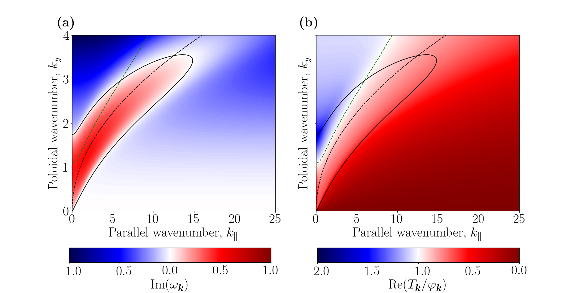
Figure 15: (a) Linear growth rate and (b) the ratio ${\text{Re}{\mathopen{}\mathclose{{}\left(T_{\boldsymbol{k}}/\varphi_{\boldsymbol{k}}}\right)}}$ of the most unstable ($k_{x}=0$) modes versus $k_{\parallel}$ and $k_{y}$ for $\kappa_{T}=1$ and $\chi=0.1$. The green dashed line is ${\text{Re}{\mathopen{}\mathclose{{}\left(T_{\boldsymbol{k}}/\varphi_{\boldsymbol{k}}}\right)}}=-1$. The black dashed line is the location of the largest collisionless growth rate $k_{\parallel}=\kappa_{T}k_{y}^{2}$. While the green and black lines would coincide to $\mathcal{O}(k_{\perp}^{-2})$ for the collisionless modes, we see that the addition of collisions shifts the linearly unstable modes towards the Dimits-favourable ${\text{Re}{\mathopen{}\mathclose{{}\left(T_{\boldsymbol{k}}/\varphi_{\boldsymbol{k}}}\right)}}>-1$ ratio.

The sensitivity of ${\text{Re}{\mathopen{}\mathclose{{}\left(T_{\boldsymbol{k}}/\varphi_{\boldsymbol{k}}}\right)}}$ to the numerical factors $a$ and $b$ allows us to carry out a simple test of the above theory. We pick a simulation that is in the Dimits state in 3D, but above the 2D Dimits threshold, i.e., has $\kappa_{T}>\kappa_{T}^{c,\text{2D}}$. We restart this simulation, but set $a=1$ for all nonzonal modes. Linearly, this increases nonzonal viscosity and reduces growth rates, without affecting zonal physics. Naïvely, one might expect that with an increased damping of the turbulence, the Dimits state should become ‘stronger’. However, such reasoning does not take into account the structure of the 3D modes and the change in the balance of Reynolds and diamagnetic stresses stemming from the change of the sign of $a+b-1$. Indeed, in this numerical experiment, we discover that the Dimits regime is destroyed and strong turbulence sets in, just as the analysis above predicts. This is clear evidence that the most consequential role of collisionality for the Dimits regime of eq. 11–eq. 13 is not to dissipate turbulent energy, but rather to regulate the turbulent stress via the ratio ${\text{Re}{\mathopen{}\mathclose{{}\left(T_{\boldsymbol{k}}/\varphi_{\boldsymbol{k}}}\right)}}$. This also suggests, for future analysis of the Dimits transition in different models of ITG turbulence, that the Dimits threshold may prove to be sensitive to the details of dissipation effects on the unstable modes, especially if, in the absence of collisions, these modes are Dimits-marginal, i.e., if they satisfy ${\text{Re}{(T_{\boldsymbol{k}}/\varphi_{\boldsymbol{k}})}}\approx-1$.

Let us also note that in the simple case of sITG modes in slab geometry, a more general calculation that includes kinetic effects is possible. In appendices G and H, we derive the kinetic sITG dispersion relation and the kinetic equivalent of eq. 53. Then, applying the ideas developed in Ivanov et al. (2020) and in this work, we show that ZF-driving small-scale sITG modes are not limited to the cold-ion limit and could play a role outside of the realm of simple fluid approximations. This, of course, can be conclusively confirmed only by appropriate GK simulations.

4.3 Breaking the Dimits state

Recall that the 2D critical gradient $\kappa_{T}^{c,\text{2D}}$ was found to be an increasing function of $\chi$. Naïvely, this makes sense on the basis of ‘more dissipation means less turbulence’: one expects that one should be able to compensate for an increase in the drive $\kappa_{T}$ by an appropriate increase in $\chi$ and thus keep the system in the Dimits state. However, this simple picture is false. Collisionality and drive are important for maintaining the Dimits state not because they provide dissipation and injection of energy, but rather because they determine the ratio ${\text{Re}{\mathopen{}\mathclose{{}\left(T_{\boldsymbol{k}}/\varphi_{\boldsymbol{k}}}\right)}}$ for the linearly unstable modes. In 2D, this ratio is sensitive to both $\kappa_{T}$ and $\chi$; however, this is not the case in 3D as the small-scale sITG modes always favour the Dimits state. First, their turbulent momentum flux was shown to satisfy ${\text{Re}{\mathopen{}\mathclose{{}\left(T_{\boldsymbol{k}}/\varphi_{\boldsymbol{k}}}\right)}}\approx-1$, with collisions pushing this ever so slightly in the Dimits-stable direction of ${\text{Re}{\mathopen{}\mathclose{{}\left(T_{\boldsymbol{k}}/\varphi_{\boldsymbol{k}}}\right)}}>-1$ (see section 4.2.5). Secondly, they provide an effective thermal diffusion for the large-scale $\mathopen{}\mathclose{{}\left\langle T}\right\rangle_{\parallel}$, which in turn reduces the absolute value of $\mathopen{}\mathclose{{}\left\langle T_{\boldsymbol{k}}}\right\rangle_{\parallel}/\mathopen{}\mathclose{{}\left\langle\varphi_{\boldsymbol{k}}}\right\rangle_{\parallel}$ and partially suppresses the tendency of large-scale modes to destroy the Dimits state (section 4.2.4). Our numerical simulations show that the combination of the mode structure of the small-scale instability and its influence on large-scale modes proves to be enough to keep the system in the Dimits regime regardless of $\kappa_{T}$ and $\chi$. As $\kappa_{T}$ increases beyond the 2D Dimits threshold $\kappa_{T}^{c,\text{2D}}$, the 2D modes flip the sign of their turbulent momentum flux and start eroding the ZFs, but the small-scale sITG modes are able to provide enough ZF drive to maintain the Dimits state (see fig. 16). Figure 17a illustrates the Dimits saturation mechanism.

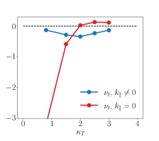
Figure 16: Dependence of the turbulent viscosity eq. 56 on the temperature gradient for $\chi=0.1$ and $L_{\parallel}=1$. The 2D Dimits regime ends at $\kappa_{T}^{c,\text{2D}}\approx 1$. In 3D simulations, the 2D modes eventually reverse their turbulent viscosity (red), but the 3D sITG modes continue to feed the ZFs through a negative turbulent viscosity (blue). The data is taken from simulations with fixed ZF profiles.

Figure 17: Schematic of the flow of energy in (a) the Dimits regime, characterised by strong, turbulence-shearing, staircase ZFs, and (b) strong turbulence, where no such ZFs can be generated or sustained. In the Dimits regime, the equilibrium gradients (EG) inject energy into large-scale modes via the 2D cITG instability. These can then drive ZFs via the secondary instability (see §2.8 of Ivanov et al., 2020) and small-scale perturbations via the parasitic sITG instability (see section 4.2). In the 2D Dimits regime ($\kappa_{T}<\kappa_{T}^{c,\text{2D}}$), the curvature-driven large-scale modes generate a negative turbulent viscosity on the ZFs and hence reinforce the Dimits state. For $\kappa_{T}>\kappa_{T}^{c,\text{2D}}$, the 2D modes erode the ZFs, but the ZF drive of the parasitic modes sustains the ZFs (see section 4.2.5). On the other hand, if a Dimits state cannot be achieved, the energy injected into the large-scale modes is transferred to small scales via the parasitic sITG instability, whence it cascades to even smaller, linearly stable scales where it is taken out of the system.

However, the small-scale sITG modes are able to maintain the Dimits state only if the 3D system is ‘3D enough’. Namely, if we restrict the system in $z$ by either squeezing it to a small $L_{\parallel}$ (see section 4.3.1) or by cutting off large-$k_{\parallel}$ modes (see section 4.3.2), we can break the ZF-dominated Dimits regime and push the system into a stongly turbulent state. The former of these methods can be deemed ‘physical’ in the sense that real system can be geometrically limited along the magnetic field, e.g., by magnetic shear. The latter is but a numerical artefact in our cold-ion system; however, parallel transport processes, which were ordered out in eq. 11–eq. 13, do provide a large-$k_{\parallel}$ cut-off for the sITG instability (see section 4.3.2).

Regardless of how the Dimits state is broken, amplitudes remain finite. The small-scale instability is able to extract energy efficiently from the large-scale ($k_{\perp}\ll 1$) fields, into which the cITG instability inputs energy, and to dump it into the small scales $k_{\perp}\gg 1$ of the sITG instability, whence it cascades to smaller scales, where dissipation can take it out of the system. Figure 17b shows the flow of energy in the strongly turbulent state.

4.3.1 Effect of parallel system size on the Dimits state

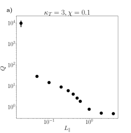
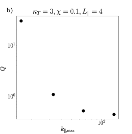
Figure 18: Dependence of the saturated turbulent heat flux $Q$ on (a) the parallel size of the box $L_{\parallel}$ and (b) the largest parallel Fourier mode $k_{\parallel,{\rm max}}$ that is included in the simulation.

Figure 18a shows a typical example of the dependence of the saturated turbulent heat flux $Q$ on the parallel size of the box $L_{\parallel}$ for parameters $\kappa_{T}$ and $\chi$ that lie beyond the 2D Dimits regime. For such parameters, the $L_{\parallel}=0$ system does not reach finite-amplitude saturation. For $L_{\parallel}$ large enough, $Q$ is independent of $L_{\parallel}$, just as it was for parameters that were within the 2D Dimits threshold (see section 4.1). As $L_{\parallel}$ is decreased, the ZFs break up and the system enters a strongly turbulent state. In fig. 18a, this happens for $L_{\parallel}<1$. As $L_{\parallel}$ approaches $0$, $Q$ starts to increase rapidly, signifying the approach to the 2D state, where a blow up occurs.

Therefore, for each pair of values of $\kappa_{T}$ and $\chi$, there exists a critical $L_{\parallel}^{\text{c}}$ such that the system is in the Dimits state for $L_{\parallel}>L_{\parallel}^{\text{c}}$ and in the strongly turbulent regime for $L_{\parallel}<L_{\parallel}^{\text{c}}$. It is clear that $L_{\parallel}^{\text{c}}=0$ if $\kappa_{T}<\kappa_{T}^{c,\text{2D}}$, i.e., if $\kappa_{T}$ and $\chi$ are such that the 2D system is able to reach saturation. The dependence of $L_{\parallel}^{\text{c}}$ on $\kappa_{T}$ and $\chi$ for $\kappa_{T}>\kappa_{T}^{c,\text{2D}}$ is not known at this point, due to the numerical cost of resolving simultaneously both the large $k_{\parallel}$ of the small-scale modes (see section 4.3.2) and the box-sized $k_{\parallel}\sim L_{\parallel}^{-1}$.

4.3.2 Effect of parallel resolution on the Dimits state

The scale separation between the large-scale cITG modes and the small-scale sITG modes increases the numerical cost of solving eq. 11–eq. 13. When the parallel resolution, i.e., the largest $k_{\parallel}$ in the simulation, is too small, the Dimits state is destroyed numerically and the system is pushed into a strong-turbulence regime for parameters for which a Dimits state would have existed if given sufficient parallel resolution. This is shown in fig. 18b. Empirically, we have found that a good rule of thumb is ‘not to chop the leaves’ of the instability, i.e., to make sure that the wavenumbers that lie within the unstable ‘leaves’ at $k_{\parallel}\sim\kappa_{T}k_{\perp}^{2}$ (see fig. 2) are fully included in the simulation. This, however, rapidly increases the numerical cost of the simulations. Recall that according to eq. 52, the collisionless sITG instability satisfies $k_{\perp}\sim(\kappa_{T}/\chi)^{1/3}$. Therefore, for a fixed $\chi$, the dimensional $k_{\parallel}$ of the unstable modes is given by

$$k_{\parallel}L_{B}\sim\kappa_{T}k_{\perp}^{2}\sim\frac{\kappa_{T}^{5/3}}{\chi^{2/3}}.$$ (82)

The number of Fourier modes required to resolve a simulation properly then scales as $\kappa_{T}^{5/3}$, in addition to scaling linearly with $L_{\parallel}$. This quickly renders numerical efforts futile, even for a fluid code.

Of course, the infinitely extending ‘leaves’ of the instability in our 3D model will, in reality, be ‘chopped off’ by phenomena that have been ordered out of our equations by eq. 3. For example, eq. 3 orders out the parallel thermal diffusion (Braginskii, 1965), but we can nonetheless estimate the dimensional $k_{\parallel}$ at which this effect will become important. This is the parallel scale at which the collisional heat conduction rate $v_{\text{th}i}^{2}k_{\parallel}^{2}/\nu_{i}$ becomes comparable to $\partial_{t}\sim c_{s}/L_{B}$ in eq. 11–eq. 13, which happens at

$$k_{\parallel}L_{B}\sim\sqrt{\frac{L_{B}}{\sqrt{\tau}\lambda_{\text{mfp}}}},$$ (83)

where $\lambda_{\text{mfp}}=v_{\text{th}i}/\nu_{i}$ is the mean-free path. In our ordering eq. 3, $\lambda_{\text{mfp}}/L_{B}\sim\tau^{3/2}$, so we find that the collisional heat conduction comes into play at $k_{\parallel}L_{B}\sim 1/\tau$. Formally, this is outside of the regime $k_{\parallel}L_{B}\sim 1$ assumed in eq. 11–eq. 13, but physically, we conclude that the Dimits regime could be broken if the collisional cut-off eq. 82 is superseded by the Braginskii scale eq. 83, i.e., if

$$\frac{L_{B}}{L_{T}}\gtrsim\mathopen{}\mathclose{{}\left(\frac{L_{B}}{\lambda_{\text{mfp}}}}\right)^{7/10}\tau^{-11/20},$$ (84)

where we used $\kappa_{T}\sim\tau L_{B}/L_{T}$ and $\chi\sim L_{B}\tau^{3/2}/\lambda_{\text{mfp}}$. In a real fusion device, this condition will not be very difficult to reach, but, in fact, the more relevant mechanism for limiting the parallel wavenumber of the sITG instability is parallel streaming rather than collisional heat conduction. In appendix G, we show that this too imposes a limit on the parallel wavenumber that is $\mathcal{O}(\tau^{-1})$ too large to be included in our ordering of $k_{\parallel}$. Namely, the sITG cut-off is given by

$$k_{\parallel}^{(c)}L_{B}=\frac{L_{B}}{2\sqrt{\pi}(1+\tau)L_{T}},$$ (85)

which supersedes the the collisional cut-off eq. 82 if

$$\frac{L_{T}}{\lambda_{\text{mfp}}}\lesssim\tau(1+\tau)^{3/2}.$$ (86)

Again, such a regime is entirely plausible for a real fusion device.

We conclude that in a more realistic physical regime than the one assumed in the derivation of our model equations eq. 11–eq. 13, the behaviour (or even existence) of parasitic sITG modes may be influenced by parallel thermal diffusion or parallel streaming in a way that breaks the Dimits regime at large enough temperature gradients.

5 Discussion

Following our analysis of the Dimits regime and its threshold in the 2D model of Ivanov et al. (2020), we have been able to extend both our model and our understanding of ITG turbulence to 3D. The important qualitative features of the 2D Dimits state, viz., strong coherent ZFs with patch-wise constant shear, turbulent bursts, and localised travelling structures survive the inclusion of 3D physics largely unchanged (see section 4.1). ZFs are generated and destroyed by the Reynolds and diamagnetic stresses of sheared ITG turbulence, respectively. If the Reynolds stress is larger, coherent ZFs can be maintained and the system settles into a low-transport Dimits state. Otherwise, a strongly turbulent, high-transport state arises in which saturation occurs unaided by ZFs. In the 2D model, the ratio of Reynolds to diamagnetic stress is sensitive to the equilibrium parameters — the temperature gradient $\kappa_{T}$ and the ion collisionality $\chi$ — and thus an appropriate balance of the two is required in order to keep the system within the Dimits regime. With the inclusion of parallel physics, however, the stresses are modified by the 3D-exclusive sITG instability, which is found always to favour the ZFs (see section 4.2.5). Unless 3D physics is restricted either by a small parallel box size (section 4.3.1) or by insufficient numerical resolution (section 4.3.2), the sITG instability is able to tip the stress balance in the Reynolds direction and a Dimits state is established regardless of the values of the equilibrium parameters.

This 3D sITG instability is found to be scale-separated from the 2D cITG instability (see section 4.2.2). In the absence of collisions, the former exists at arbitrarily small perpendicular and parallel scales, while the latter is confined to large scales. This scale separation allows for sITG modes that are predominantly driven not by the equilibrium gradients but rather by the local gradients of large-scale fields, which are themselves driven by the equilibrium gradients (i.e., the sITG instability is parasitic). The nonlinear energy transfer from large-scale to small-scale modes that results from the sITG instability is found to have the form of an effective large-scale thermal diffusion (see section 4.2.4). The combination of this thermal diffusion and the favourable turbulent stress of the small-scale modes are what makes the 3D Dimits state much more resilient than its 2D counterpart.

The fact that the Dimits state is governed by essentially the same physical mechanisms in both the 2D and 3D cold-ion $Z$-pinch systems gives us not only hope that one day we could understand the Dimits regime of full-blown GK, but also a solid foundation of numerical and analytical work upon which to build such an undertaking. Although there is some numerical evidence of important similarities between these simple systems and GK, e.g., the ferdinon structures seen both by us and by van Wyk et al. (2016, 2017) in their GK simulations of an experimentally realistic configuration, there is still much unknown. The details of the Dimits state in our 3D model depend on certain peculiar features of cold-ion physics. It is the cold-ion approximation that permits the parasitic small-scale sITG instability that underlies the main differences between the 2D and 3D models. As this is only one asymptotic limit of GK, it is difficult to extrapolate any quantitative predictions. However, it is important to note that the kinetic, $\tau\sim 1$, dispersion relation also predicts a collisionless sITG instability at arbitrarily large $k_{\perp}$ (see appendix G), as was already established by Smolyakov et al. (2002). Just as in the cold-ion fluid model, these sITG modes appear to favour a ZF-dominated state (appendix H). Thus, the appearance of parasitic modes is not necessarily limited to our cold-ion model and, in certain regimes, could also be a feature of low-collisionality GK. This may also require a careful investigation of GK collisions along the lines of Frei et al. (2022). All of this, combined with the fact that the nature of the Dimits state in the 2D and 3D models is essentially the same, encourages us to carry our ideas over into the vastly more complex world of GK. At this point, it is unknown whether the Reynolds–diamagnetic stress competition is also behind the Dimits transition in GK. One of the prominent alternative ideas is the primary-secondary-tertiary scenario, first proposed by Rogers et al. (2000). Recently, there have been a number of publications discussing the applicability of this paradigm to both fluid and kinetic models (St-Onge, 2017; Zhu et al., 2018, 2020a, 2020b; Hallenbert & Plunk, 2021). Note that, as we showed in Ivanov et al. (2020), the Dimits transition that we observe cannot be explained by the tertiary instability of ZFs. It is possible that the nature of the transition to high transport in realistic GK simulations is, in fact, not as clear-cut as it is in the simple models, but is rather a combination of both mechanisms, viz., the competition between the stresses and a tertiary instability.

Another important feature that our model lacks is magnetic shear. It is well-known that this can have a significant effect on both the linear instabilities and turbulence levels in realistic-geometry GK simulations (Kinsey et al., 2006). Notably, much effort today is being devoted to spherical tokamak designs, which can have large values of field-line-averaged magnetic shear combined with nontrivial variations in the local shear. Therefore, we consider the addition of magnetic shear to our analytical and numerical models to be a key direction for future work.

Declaration of interests

The authors report no conflict of interest.

Appendix A Derivation of the 3D model

We follow the derivation in Appendix A of Ivanov et al. (2020), but retain the parallel-streaming term in the GK equation. For the sake of brevity, we shall use the notation and definitions of Ivanov et al. (2020).

The electrostatic ion GK equation is

$$\frac{\partial}{\partial t}\mathopen{}\mathclose{{}\left(h-\mathopen{}\mathclose{{}\left\langle\varphi}\right\rangle_{\boldsymbol{R}}F_{i}}\right)+{v_{\parallel}}\partial_{\parallel}h+\frac{\rho_{i}v_{\text{th}i}}{2L_{T}}\mathopen{}\mathclose{{}\left(\frac{v^{2}}{v^{2}_{ti}}-\frac{3}{2}}\right)F_{i}\frac{\partial\mathopen{}\mathclose{{}\left\langle\varphi}\right\rangle_{\boldsymbol{R}}}{\partial Y}-\frac{\rho_{i}v_{\text{th}i}}{L_{B}}\mathopen{}\mathclose{{}\left(\frac{v^{2}_{\parallel}}{v_{\text{th}i}^{2}}+\frac{v^{2}_{\perp}}{2v_{\text{th}i}^{2}}}\right)\frac{\partial h}{\partial Y}$$

$$\quad+\frac{1}{2}\rho_{i}v_{\text{th}i}\mathopen{}\mathclose{{}\left\{\mathopen{}\mathclose{{}\left\langle\varphi}\right\rangle_{\boldsymbol{R}},h}\right\}=\mathopen{}\mathclose{{}\left\langle C_{l}[h]}\right\rangle_{\boldsymbol{R}},$$ (87)

closed via the quasineutrality condition and eq. 1:

$$\frac{1}{n_{i}}\int d^{3}{\boldsymbol{v}}\ \mathopen{}\mathclose{{}\left\langle h}\right\rangle_{\boldsymbol{r}}=\varphi+\tau\varphi^{\prime}.$$ (88)

The 2D fluid model was derived in a highly collisional ($\partial_{t}\ll\nu_{i}$), cold-ion ($\tau\ll 1$), long-wavelength ($k_{\perp}^{2}\rho_{i}^{2}\ll 1$) limit of the ion GK equation that obeys eq. 3. Note that, as discussed in section 2, in order to retain the sITG instability in the final equations, we need to order $\partial_{\parallel}\sim L_{B}^{-1}$. Thus, the parallel-streaming term is ordered as

$${v_{\parallel}}\partial_{\parallel}h\sim\frac{v_{\text{th}i}}{L_{B}}h\ll\partial_{t}h\sim\frac{c_{s}}{L_{B}}h\sim\frac{v_{\text{th}i}}{L_{B}\sqrt{\tau}}h,$$ (89)

i.e., it is one order of $\sqrt{\tau}$ smaller than the $\partial_{t}h$ term. This means that here we need to expand the distribution function in $\sqrt{\tau}$, rather than in $\tau$, as was done in Ivanov et al. (2020). In order to be consistent with the notation of our 2D derivation, we set $h=h^{(0)}+h^{(1/2)}+h^{(1)}+...$, where $h^{(1/2)}\sim\sqrt{\tau}h^{(0)}$, etc.

A.1 Lowest-order solution

To order $\mathcal{O}(\sqrt{\tau})$, the ion GK equation appendix A is dominated by collisions, viz.,

$$C_{l}[h^{(0)}+h^{(1/2)}]=0.$$ (90)

The solution to this equation is a perturbed Maxwellian distribution (Newton et al., 2010):

$$h^{(0)}+h^{(1/2)}=\mathopen{}\mathclose{{}\left[\frac{\delta N}{n_{i}}+\frac{\delta T}{T_{i}}\mathopen{}\mathclose{{}\left(\frac{v^{2}}{v_{\text{th}i}^{2}}-\frac{3}{2}}\right)+\frac{2{v_{\parallel}}u_{\parallel}}{v_{\text{th}i}^{2}}}\right]F_{i}.$$ (91)

Here $\delta T/T_{i}$ will turn out to be just the ion temperature perturbation, while the density-like quantity $\delta N/n_{i}$ is

$$\frac{\delta N}{n_{i}}=\varphi+\tau\varphi^{\prime}-\frac{1}{4}\rho_{i}^{2}\nabla_{\perp}^{2}\mathopen{}\mathclose{{}\left(\varphi+\frac{\delta T}{T_{i}}}\right)+\mathcal{O}\mathopen{}\mathclose{{}\left(k_{\perp}^{4}\rho_{i}^{4}\varphi}\right).$$ (92)

For more details, see the derivations in Ivanov et al. (2020). The ordering $u_{\parallel}\sim\tau c_{s}\varphi$, which we established using eq. 8, implies that

$$\frac{2{v_{\parallel}}u_{\parallel}}{v_{\text{th}i}^{2}}\sim\frac{\tau c_{s}\varphi}{v_{\text{th}i}}\sim\sqrt{\tau}\varphi.$$ (93)

Therefore, the perturbed parallel flow does not enter into $h^{(0)}$. We define solution for the distribution function to two lowest orders as

$$h^{(0)}=\mathopen{}\mathclose{{}\left[\frac{\delta N}{n_{i}}+\frac{\delta T}{T_{i}}\mathopen{}\mathclose{{}\left(\frac{v^{2}}{v_{\text{th}i}^{2}}-\frac{3}{2}}\right)}\right]F_{i},$$ (94)

$$h^{(1/2)}=\frac{2{v_{\parallel}}u_{\parallel}}{v_{\text{th}i}^{2}}F_{i},$$ (95)

and the solubility conditions

$${\int d^{3}{\boldsymbol{v}}\ }h^{(n)}={\int d^{3}{\boldsymbol{v}}\ }v^{2}h^{(n)}={\int d^{3}{\boldsymbol{v}}\ }{v_{\parallel}}h^{(n)}=0$$ (96)

for $n\geq 1$.

Note that our expansion implies that parallel collisional effects (parallel heat flux and parallel viscosity) enter via $h^{(3/2)}$ and so are asymptotically too small to appear in any of our fluid equations.

A.2 Fluid equations

We proceed by taking the density, temperature, and parallel-velocity moments of appendix A. The derivation for the ‘two-dimensional parts’ of the equations for $\varphi$ and $T$ can be found in Ivanov et al. (2020).

The density moment at fixed particle position, $(1/n_{i})\int d^{3}{\boldsymbol{v}}\ \mathopen{}\mathclose{{}\left\langle.}\right\rangle_{\boldsymbol{r}}$, of appendix A is

$$\frac{\partial}{\partial t}\mathopen{}\mathclose{{}\left(\tau\varphi^{\prime}-\frac{1}{2}\rho_{i}^{2}\nabla_{\perp}^{2}\varphi}\right)+\int d^{3}{\boldsymbol{v}}\ {v_{\parallel}}\partial_{\parallel}\mathopen{}\mathclose{{}\left\langle h^{(1/2)}}\right\rangle_{\boldsymbol{r}}-\frac{\rho_{i}v_{\text{th}i}}{L_{B}}\frac{\partial}{\partial y}\mathopen{}\mathclose{{}\left(\varphi+T}\right)+\frac{\rho_{i}v_{\text{th}i}}{2L_{T}}\frac{\partial}{\partial y}\mathopen{}\mathclose{{}\left(\frac{1}{2}\rho_{i}^{2}\nabla_{\perp}^{2}\varphi}\right)$$ (97)

$$\quad+\frac{1}{2}\rho_{i}v_{\text{th}i}\bigg{(}\mathopen{}\mathclose{{}\left\{\varphi,\tau\varphi^{\prime}-\frac{1}{2}\rho_{i}^{2}\nabla_{\perp}^{2}\varphi}\right\}+\frac{1}{2}\rho_{i}^{2}\boldsymbol{\nabla_{\perp}}\bcdot\mathopen{}\mathclose{{}\left\{\boldsymbol{\nabla_{\perp}}\varphi,T}\right\}\bigg{)}$$

$$\quad=-\frac{1}{2}\chi\rho_{i}^{2}\nabla_{\perp}^{4}(a\varphi-bT),$$ (98)

where all terms are of order $\mathcal{O}(\tau h^{(0)})$. The parallel-velocity moment is, using eq. 95,

$$\frac{1}{n_{i}}\int d^{3}{\boldsymbol{v}}\ {v_{\parallel}}\partial_{\parallel}\mathopen{}\mathclose{{}\left\langle h^{(1/2)}}\right\rangle_{\boldsymbol{r}}\approx\partial_{\parallel}u_{\parallel}.$$ (99)

Combining eq. 99 with eq. 97 yields eq. 4.

Similarly, the temperature moment, $(1/n_{i})\int d^{3}{\boldsymbol{v}}\ v^{2}/v_{\text{th}i}^{2}\mathopen{}\mathclose{{}\left\langle.}\right\rangle_{\boldsymbol{r}}$, of appendix A is

$$\frac{\partial T}{\partial t}+\frac{1}{n_{i}}\int d^{3}{\boldsymbol{v}}{v_{\parallel}}\partial_{\parallel}\frac{v^{2}}{v_{\text{th}i}^{2}}\mathopen{}\mathclose{{}\left\langle h^{(1/2)}}\right\rangle_{\boldsymbol{r}}+\frac{\rho_{i}v_{\text{th}i}}{2L_{T}}\frac{\partial\varphi}{\partial y}+\frac{1}{2}\rho_{i}v_{\text{th}i}\mathopen{}\mathclose{{}\left\{\varphi,T}\right\}=\chi\nabla_{\perp}^{2}T,$$ (100)

where the parallel-streaming term is

$$\frac{1}{n_{i}}\int d^{3}{\boldsymbol{v}}{v_{\parallel}}\partial_{\parallel}\frac{v^{2}}{v_{\text{th}i}^{2}}\mathopen{}\mathclose{{}\left\langle h^{(1/2)}}\right\rangle_{\boldsymbol{r}}=\frac{5}{2}\partial_{\parallel}u_{\parallel}.$$ (101)

Hence we obtain section 2.1.

Finally, we take the parallel-velocity moment, $(1/n_{i})\int d^{3}{\boldsymbol{v}}\ {v_{\parallel}}\mathopen{}\mathclose{{}\left\langle.}\right\rangle_{\boldsymbol{r}}$, of appendix A. The first term is the time derivative of

$$\frac{1}{n_{i}}\int d^{3}{\boldsymbol{v}}\ {v_{\parallel}}\mathopen{}\mathclose{{}\left\langle h-\mathopen{}\mathclose{{}\left\langle\varphi}\right\rangle_{\boldsymbol{R}}F_{i}}\right\rangle_{\boldsymbol{r}}\approx\frac{1}{n_{i}}\int d^{3}{\boldsymbol{v}}\ {v_{\parallel}}h^{(1/2)}=u_{\parallel}.$$ (102)

The parallel-streaming term is

$$\frac{1}{n_{i}}\int d^{3}{\boldsymbol{v}}\ v_{\parallel}^{2}\partial_{\parallel}\mathopen{}\mathclose{{}\left\langle h}\right\rangle_{\boldsymbol{r}}\approx\frac{1}{n_{i}}\int d^{3}{\boldsymbol{v}}\ v_{\parallel}^{2}\partial_{\parallel}h^{(0)}=\frac{1}{2}v_{\text{th}i}^{2}\partial_{\parallel}(\varphi+T).$$ (103)

The temperature-gradient term integrates to 0 because the integrand is odd in ${v_{\parallel}}$. The magnetic-gradient term is one order of $L_{T}/L_{B}\sim\mathcal{O}(\tau)\ll 1$ smaller than the rest (the magnetic curvature is absent from eq. 100 for the same reason). The nonlinear term integrates to

$$\frac{1}{n_{i}}\int d^{3}{\boldsymbol{v}}\ {v_{\parallel}}\mathopen{}\mathclose{{}\left\langle\mathopen{}\mathclose{{}\left\{\mathopen{}\mathclose{{}\left\langle\varphi}\right\rangle_{\boldsymbol{R}},h}\right\}}\right\rangle_{\boldsymbol{r}}\approx\frac{1}{n_{i}}\int d^{3}{\boldsymbol{v}}\ {v_{\parallel}}\mathopen{}\mathclose{{}\left\{\varphi,h^{(1/2)}}\right\}=\frac{1}{2}\rho_{i}v_{\text{th}i}\mathopen{}\mathclose{{}\left\{\varphi,u_{\parallel}}\right\}.$$ (104)

Finally, the parallel-velocity moment of the collisional operator is

$$\frac{1}{n_{i}}\int d^{3}{\boldsymbol{v}}\ {v_{\parallel}}\mathopen{}\mathclose{{}\left\langle\mathopen{}\mathclose{{}\left\langle C_{l}[h]}\right\rangle_{\boldsymbol{R}}}\right\rangle_{\boldsymbol{r}}\approx\frac{1}{n_{i}}\int d^{3}{\boldsymbol{v}}\ {v_{\parallel}}C_{l}[h^{(1/2)}]=s\nabla_{\perp}^{2}u_{\parallel},$$ (105)

where $s=9/10$ is a numerical factor (see Newton et al., 2010). Putting together eq. 102–eq. 105, we arrive at eq. 6.

Appendix B Slab-ITG instability condition

Here we derive the instability boundaries eq. 32 for the dispersion relation eq. 31. Note that the left-hand side of eq. 31 is a cubic polynomial in $\hat{\omega}_{\boldsymbol{k}}$ with one positive and two negative roots, while the right-hand side is a simple quadratic propotional to $\hat{\omega}_{\boldsymbol{k}}^{2}$ (see fig. 19). First, if $\hat{\gamma}_{\boldsymbol{k}}^{2}<0$, then the right-hand side is a concave parabola and it is geometrically evident that there will always be three intersections of the parabola and the cubic, and so there are no unstable solutions. On the other hand, if $\hat{\gamma}_{\boldsymbol{k}}^{2}>0$, then these two curves cross three times if and only if the cubic left-hand side is larger than the quadratic right-hand side at $\hat{\omega}_{\boldsymbol{k}}=\hat{\omega}_{\boldsymbol{k}}^{(0)}<0$, where the two curves have the same slope. We differentiate eq. 31 to find that $\hat{\omega}_{\boldsymbol{k}}^{(0)}$ is the negative solution to

$$\mathopen{}\mathclose{{}\left(\hat{\omega}_{\boldsymbol{k}}^{(0)}}\right)^{2}+\mathopen{}\mathclose{{}\left[\frac{2}{3}-\frac{4k_{\perp}^{2}\hat{\gamma}_{\boldsymbol{k}}^{2}}{3(1+k_{\perp}^{2})}}\right]\hat{\omega}_{\boldsymbol{k}}^{(0)}-\frac{1}{3}\frac{k_{\parallel}^{2}}{1+k_{\perp}^{2}}=0.$$ (106)

Using eq. 106 to substitute for $\hat{\omega}_{\boldsymbol{k}}^{(0)}$, the instability condition that the left-hand side of eq. 31 be smaller than its right-hand side is then found to be equivalent to

$$\hat{\omega}_{\boldsymbol{k}}^{(0)}>-\hat{k}_{\parallel}^{2}\frac{4(1+k_{\perp}^{2})+k_{\perp}^{2}\hat{\gamma}_{\boldsymbol{k}}^{2}}{3\hat{k}_{\parallel}^{2}(1+k_{\perp}^{2})+\mathopen{}\mathclose{{}\left(1+k_{\perp}^{2}-2k_{\perp}^{2}\hat{\gamma}_{\boldsymbol{k}}^{2}}\right)^{2}}\equiv\hat{\omega}_{\boldsymbol{k}}^{\text{min}}.$$ (107)

Since $\hat{\omega}_{\boldsymbol{k}}^{(0)}$ is the negative solution of the quadratic eq. 106 and $\hat{\omega}_{\boldsymbol{k}}^{\text{min}}<0$, eq. 107 can be true if and only if the quadratic eq. 106 is positive when we substitute $\hat{\omega}_{\boldsymbol{k}}^{\text{min}}$ for $\hat{\omega}_{\boldsymbol{k}}^{(0)}$. Performing that substitution and simplifying the resulting expression yields a quadratic inequality for $\hat{k}_{\parallel}^{2}$:

$$-(1+k_{\perp}^{2})\hat{k}_{\parallel}^{4}+\hat{k}_{\parallel}^{2}\mathopen{}\mathclose{{}\left[2(1+k_{\perp}^{2})^{2}+10k_{\perp}^{2}\hat{\gamma}_{\boldsymbol{k}}^{2}(1+k_{\perp}^{2})-k_{\perp}^{4}\hat{\gamma}_{\boldsymbol{k}}^{4}}\right]-(1+k_{\perp}^{2}-2k_{\perp}^{2}\hat{\gamma}_{\boldsymbol{k}}^{2})^{3}>0.$$ (108)

Its solution is the interval $\hat{k}_{\parallel}^{2}\in(\hat{k}_{\parallel,-}^{2},\hat{k}_{\parallel,+}^{2})$, where $\hat{k}_{\parallel,\pm}^{2}$ are given by eq. 32.

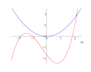
Figure 19: The left-hand (red) and right-hand (blue) sides of the sITG dispersion relation eq. 31 for $\hat{k}_{\parallel}=2$, $k_{\perp}^{2}=0.2$. There is only one real solution, so there exists a complex one with positive imaginary part. Thus, there are linearly unstable modes for $\hat{k}_{\parallel}=2$, $k_{\perp}^{2}=0.2$.

Appendix C Collisional slab instability

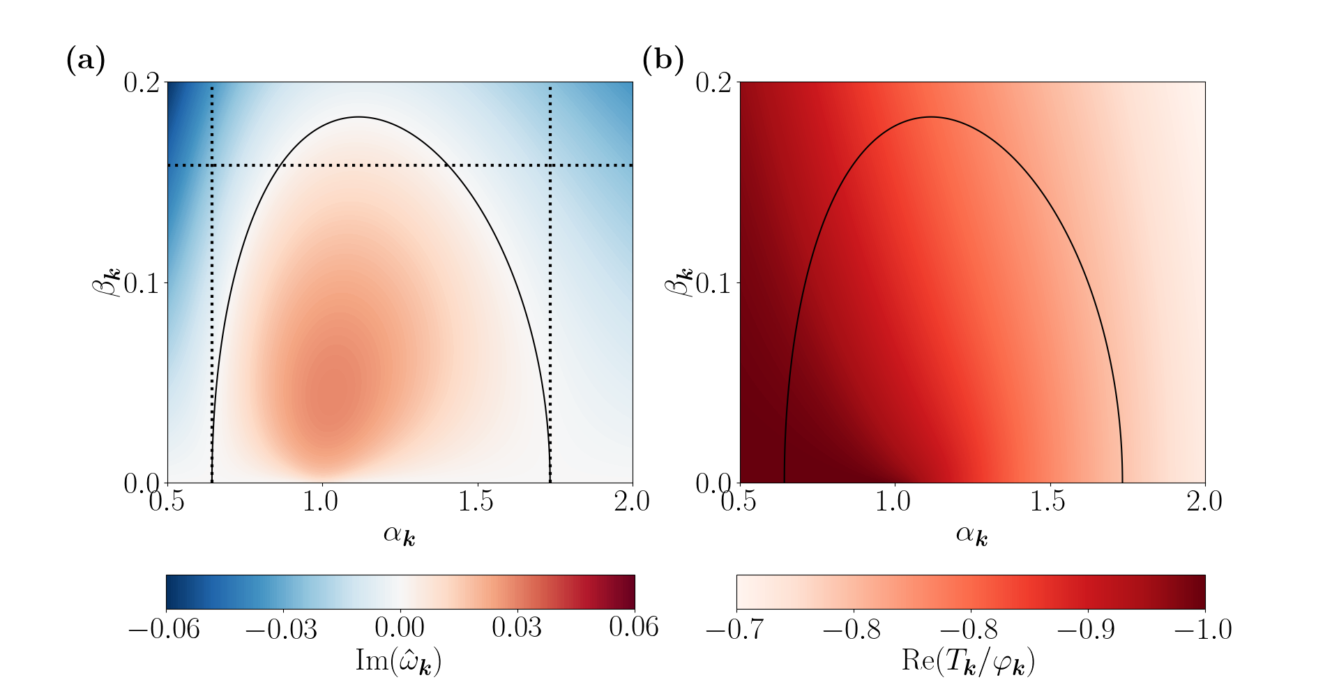
Figure 20: (a) Largest growth rate ${\text{Im}{(\hat{\omega}_{\boldsymbol{k}})}}$ obtained by solving eq. 109. (b) The ratio ${\text{Re}{(T_{\boldsymbol{k}}/\varphi_{\boldsymbol{k}})}}$ for the most unstable mode. The solid black line is the stability boundary ${\text{Im}{(\hat{\omega}_{\boldsymbol{k}})}}=0$. The dotted lines in (a) show the analytic approximations to the $\alpha_{\boldsymbol{k}}$ and $\beta_{\boldsymbol{k}}$ instability boundaries, given by eq. 112 (for $\beta_{\boldsymbol{k}}\ll 1$) and eq. 118 (for $\beta_{\boldsymbol{k}}\sim\lambda\ll 1$). We see perfect agreement with eq. 112, but a slight discrepancy with eq. 118, whose derivation is accurate only under the assumption that $1-a-b=\lambda\approx 0.36$ is small. All unstable modes lie within ${\text{Re}{(T_{\boldsymbol{k}}/\varphi_{\boldsymbol{k}})}}>-1$.

To simplify the dispersion relation and focus on the $\chi$ITG instability promised at the end of section 3.4, let us consider the $k_{\perp}\gg 1$ limit of eq. 46–eq. 48, i.e., drop the $\partial_{t}\varphi^{\prime}$ term in eq. 46, and also drop the collisionless-resonance term $\partial_{t}\varphi^{\prime}$ from the right-hand side of eq. 47. The dispersion relation for the thus simplified equations becomes

$$(\hat{\omega}_{\boldsymbol{k}}+1)(\hat{\omega}_{\boldsymbol{k}}+is\beta_{\boldsymbol{k}})(\hat{\omega}_{\boldsymbol{k}}+i\beta_{\boldsymbol{k}})-\alpha_{\boldsymbol{k}}(\hat{\omega}_{\boldsymbol{k}}+1+i\beta_{\boldsymbol{k}})+i\beta_{\boldsymbol{k}}(\hat{\omega}_{\boldsymbol{k}}+is\beta_{\boldsymbol{k}})(a\hat{\omega}_{\boldsymbol{k}}+ia\beta_{\boldsymbol{k}}-b)=0,$$ (109)

where we have defined $\hat{\omega}_{\boldsymbol{k}}\equiv\omega_{\boldsymbol{k}}/\kappa_{T}k_{y}$, $\alpha_{\boldsymbol{k}}\equiv k_{\parallel}^{2}/\kappa_{T}^{2}k_{y}^{2}k_{\perp}^{2}$, $\beta_{\boldsymbol{k}}\equiv\chi{k_{\perp}^{2}}/\kappa_{T}k_{y}$. Note that the five parameters of a Fourier mode, viz., $\kappa_{T}$, $\chi$, and the three components of ${\boldsymbol{k}}$ have collapsed into only two effective parameters: $\alpha_{\boldsymbol{k}}$ and $\beta_{\boldsymbol{k}}$. Thus, we only need to solve eq. 109 in the $(\alpha_{\boldsymbol{k}},\beta_{\boldsymbol{k}})$ plane. The solution (in particular, its imaginary part) is shown in fig. 20, alongside the value of ${\text{Re}{(T_{\boldsymbol{k}}/\varphi_{\boldsymbol{k}})}}$ for the most unstable mode — a quantity that is crucial for the Dimits regime (see section 4.1 and also Ivanov et al., 2020). Let us discuss this solution in some easy limits.

First, consider the case of $\beta_{\boldsymbol{k}}\ll 1\sim\alpha_{\boldsymbol{k}}$. As $\beta_{\boldsymbol{k}}\sim k_{\perp}$, this limit corresponds to the low-$k_{\perp}$ end of the wavenumber spectrum of the collisional instability. Note that this is a subsidiary expansion to the $k_{\perp}\gg 1$ one used to obtain eq. 109. To lowest order in $\beta_{\boldsymbol{k}}$, eq. 109 yields

$$(\hat{\omega}_{\boldsymbol{k}}^{2}-\alpha_{\boldsymbol{k}})(\hat{\omega}_{\boldsymbol{k}}+1)=0,$$ (110)

whence $\hat{\omega}_{\boldsymbol{k}}\approx\hat{\omega}_{\boldsymbol{k}}^{(0)}=-1,\pm\sqrt{\alpha_{\boldsymbol{k}}}$. Letting $\hat{\omega}_{\boldsymbol{k}}=\hat{\omega}_{\boldsymbol{k}}^{(0)}+\delta\hat{\omega}_{\boldsymbol{k}}$, where $\delta\hat{\omega}_{\boldsymbol{k}}/\hat{\omega}_{\boldsymbol{k}}\sim\beta_{\boldsymbol{k}}\ll 1$, we find in the next order

$$\hat{\omega}_{\boldsymbol{k}}=-1+\frac{-i\beta_{\boldsymbol{k}}(a+b-\alpha_{\boldsymbol{k}})}{1-\alpha_{\boldsymbol{k}}},\ \pm\sqrt{\alpha_{\boldsymbol{k}}}+\frac{-i\beta_{\boldsymbol{k}}\mathopen{}\mathclose{{}\left[\sqrt{\alpha_{\boldsymbol{k}}}(s+a)\pm(s+1-b)}\right]}{2(\sqrt{\alpha_{\boldsymbol{k}}}\pm 1)}.$$ (111)

It is then evident that the $\hat{\omega}_{\boldsymbol{k}}^{(0)}=\sqrt{\alpha_{\boldsymbol{k}}}$ solution is always stable, while the other two give the following condition for instability:

$$\alpha_{\boldsymbol{k}}=\frac{k_{\parallel}^{2}}{\kappa_{T}^{2}k_{y}^{2}k_{\perp}^{2}}\in\mathopen{}\mathclose{{}\left(a+b,\mathopen{}\mathclose{{}\left(\frac{s+1-b}{s+a}}\right)^{2}}\right)\approx(0.64,1.73),$$ (112)

the numerical values being valid for $a$, $b$, and $s$ as given after eq. 7. The instability boundaries in eq. 112 agree with fig. 20. Note that for $a+b\to 1$, eq. 112 implies that $\alpha_{\boldsymbol{k}}\to 1$, i.e., $k_{\parallel}\to\kappa_{T}k_{y}k_{\perp}$, which is precisely the resonance condition we discovered in section 3.4. In hindsight, this is expected because the collisional coupling term on the right-hand side of eq. 47 goes to zero in the limit $a+b\to 1$.

Equation eq. 111 implies that the growth rate ${\text{Im}{(\hat{\omega}_{\boldsymbol{k}})}}$ of the $\beta_{\boldsymbol{k}}\ll 1$ collisional modes satisfies ${\text{Im}{(\hat{\omega}_{\boldsymbol{k}})}}\sim\beta_{\boldsymbol{k}}$. However, these expressions break down when $\alpha_{\boldsymbol{k}}=1+\mathcal{O}(\beta_{\boldsymbol{k}})$. We now show that this is precisely where the fastest-growing mode resides, similarly to what we found in section 3.3.2 for the collisionless sITG mode. Setting $\hat{\omega}_{\boldsymbol{k}}=-1+\delta\hat{\omega}_{\boldsymbol{k}}$, $\alpha_{\boldsymbol{k}}=1+\delta\alpha_{\boldsymbol{k}}$, where $\delta\hat{\omega}_{\boldsymbol{k}}\sim\delta\alpha_{\boldsymbol{k}}\sim\sqrt{\beta_{\boldsymbol{k}}}\ll 1$, we find from eq. 109 that

$$2\delta\hat{\omega}_{\boldsymbol{k}}^{2}+\delta\alpha_{\boldsymbol{k}}+i(a+b-1)\beta_{\boldsymbol{k}}=0\implies{\text{Im}{\mathopen{}\mathclose{{}\left(\hat{\omega}_{\boldsymbol{k}}}\right)}}=\pm\frac{\sqrt{\delta\alpha_{\boldsymbol{k}}^{2}-8i(a+b-1)\beta_{\boldsymbol{k}}}}{4},$$ (113)

which implies that ${\text{Im}{\mathopen{}\mathclose{{}\left(\hat{\omega}_{\boldsymbol{k}}}\right)}}$ is largest when $\delta\alpha_{\boldsymbol{k}}=0$. To see this, note that the imaginary part of the square root of a complex number $u+iv$ is equal to

$${\text{Im}{\mathopen{}\mathclose{{}\left(\sqrt{u+iv}}\right)}}=\sqrt{\frac{-u+\sqrt{u^{2}+v^{2}}}{2}},$$ (114)

which can easily be shown to be a decreasing function of $u$. Therefore, the growth rate in eq. 113 is largest when $\delta\alpha_{\boldsymbol{k}}=0$ and is given by

$${\text{Im}{\mathopen{}\mathclose{{}\left(\hat{\omega}_{\boldsymbol{k}}}\right)}}=\frac{1}{2}\sqrt{|a+b-1|\beta_{\boldsymbol{k}}},$$ (115)

so it scales as ${\text{Im}{\mathopen{}\mathclose{{}\left(\hat{\omega}_{\boldsymbol{k}}}\right)}}\sim\sqrt{\beta_{\boldsymbol{k}}}$. Note that this growth rate vanishes when $a+b=1$, i.e., when the instability boundaries eq. 112 lie on top of each other.

The growth rate given by eq. 115 is comparable to the collisionless growth rate eq. 44 when $\kappa_{T}k_{y}\sqrt{\beta_{\boldsymbol{k}}}\sim\kappa_{T}$, i.e., when $k_{\perp}\sim(\kappa_{T}/\chi)^{1/3}$, where we assumed $k_{y}\sim k_{\perp}$. This is precisely the condition $k_{\perp}\sim k_{\chi}$ for the transition from the collisionless to the collisional regime that we found in section 3.4.

In the opposite limit of $\beta_{\boldsymbol{k}}\gg 1\sim\alpha_{\boldsymbol{k}}$, eq. 109 gives

$$\hat{\omega}_{\boldsymbol{k}}^{3}+i(s+a+1)\beta_{\boldsymbol{k}}\hat{\omega}_{\boldsymbol{k}}^{2}-(s+a+as)\beta_{\boldsymbol{k}}^{2}\hat{\omega}_{\boldsymbol{k}}-ias\beta_{\boldsymbol{k}}^{3}=0,$$ (116)

which has three stable solutions: $\hat{\omega}_{\boldsymbol{k}}=-i\beta_{\boldsymbol{k}},-ia\beta_{\boldsymbol{k}},-is\beta_{\boldsymbol{k}}$. We can therefore conclude that there exists a $\beta_{\text{max}}\sim 1$ such that unstable solutions are possible only for $\beta_{\boldsymbol{k}}<\beta_{\text{max}}$. A simple analytical estimate for $\beta_{\text{max}}$ is obtainable if we make an additional approximation: let $\lambda\equiv 1-a-b\ll 1$ and consider an expansion in small $\lambda$. In this limit, the collisional coupling in eq. 47 is small and eq. 112 requires $\alpha_{\boldsymbol{k}}=1+\mathcal{O}(\lambda)$. We let $\hat{\omega}_{\boldsymbol{k}}=-1+\delta\hat{\omega}_{\boldsymbol{k}}$, $\alpha_{\boldsymbol{k}}=1+\delta\alpha_{\boldsymbol{k}}$, where $\delta\hat{\omega}_{\boldsymbol{k}}\sim\delta\alpha_{\boldsymbol{k}}\sim\beta_{\boldsymbol{k}}\sim\lambda\ll 1$, and expand eq. 109 to $\mathcal{O}(\lambda)$ to find

$$\delta\hat{\omega}_{\boldsymbol{k}}=\frac{-\delta\alpha_{\boldsymbol{k}}-i\beta_{\boldsymbol{k}}(a+s+2)\pm\sqrt{\mathopen{}\mathclose{{}\left[\delta\alpha_{\boldsymbol{k}}+i\beta_{\boldsymbol{k}}(a+s+2)}\right]^{2}-8i\beta_{\boldsymbol{k}}(\lambda+\delta\alpha_{\boldsymbol{k}})+8(a+s)\beta_{\boldsymbol{k}}^{2}}}{4}.$$ (117)

After some unenlightening algebra, we find that eq. 117 supports unstable solutions for

$$\beta_{\boldsymbol{k}}<\beta_{\text{max}}\approx\frac{\lambda}{2(a+s)}=\frac{1-a-b}{2(a+s)}\approx 0.16,$$ (118)

which is in reasonable agreement with the numerically determined $\beta_{\text{max}}\approx 0.18$.

Numerically, we find that the fastest-growing mode is located at $\beta_{\text{fastest}}\approx 0.04$, $\alpha\approx 1.01$, and has a growth rate ${\text{Im}{(\hat{\omega}_{\boldsymbol{k}})}}=\hat{\gamma}_{\text{fastest}}\approx 0.03$. The dependence of ${\text{Im}{(\hat{\omega}_{\boldsymbol{k}})}}$ on $\alpha_{\boldsymbol{k}}$ and $\beta_{\boldsymbol{k}}$ is shown in fig. 20. Undoing the normalisations of $\alpha_{\boldsymbol{k}}$, $\beta_{\boldsymbol{k}}$, and $\hat{\omega}_{\boldsymbol{k}}$, we find that this collisional instability is localised at $k_{\parallel}\approx\kappa_{T}k_{y}k_{\perp}$ (just as the collisionless modes are), is bounded by $\beta_{\text{max}}\approx 0.18>\beta$, and has its largest growth rate

$${\text{Im}{(\omega_{\boldsymbol{k}})}}=\kappa_{T}k_{y}\gamma_{\text{fastest}}\approx 0.03\kappa_{T}k_{y}\ \ \text{at}\ \ \frac{{k_{\perp}^{2}}}{k_{y}}=\frac{\beta_{\text{fastest}}\kappa_{T}}{\chi}\approx\frac{0.04\kappa_{T}}{\chi}.$$ (119)

As $\hat{\omega}_{\boldsymbol{k}}$ depends on ${\boldsymbol{k}}_{\perp}$ through $\beta_{\boldsymbol{k}}$, the contours of constant $\hat{\omega}_{\boldsymbol{k}}$ in the $(k_{x},k_{y})$ plane coincide with those of constant $\beta_{\boldsymbol{k}}$. Since $\beta_{\boldsymbol{k}}=\chi{k_{\perp}^{2}}/\kappa_{T}k_{y}$, these are circles with radius $\kappa_{T}\beta_{\boldsymbol{k}}/2\chi$, centred at $k_{x}=0$ and $k_{y}=\kappa_{T}\beta_{\boldsymbol{k}}/2\chi$. Since $\omega_{\boldsymbol{k}}=\kappa_{T}k_{y}\hat{\omega}_{\boldsymbol{k}}$, the largest ${\text{Im}{(\omega_{\boldsymbol{k}})}}$ for a given $\beta_{\boldsymbol{k}}$ is found at $k_{x}=0$ and $k_{y}=\kappa_{T}\beta_{\boldsymbol{k}}/\chi$. In particular, the most unstable mode has

$$k_{y}=\frac{\beta_{\text{fastest}}\kappa_{T}}{\chi}\approx\frac{0.04\kappa_{T}}{\chi},\quad{\text{Im}{\mathopen{}\mathclose{{}\left(\omega_{\boldsymbol{k}}}\right)}}\approx 0.0012\frac{\kappa_{T}^{2}}{\chi}.$$ (120)

The growth rate eq. 120 scales quadratically with $\kappa_{T}$, unlike the collisionless sITG instabilities considered in section 3.3, and also diverges as $\chi\to 0$. Therefore, either for sufficiently large $\kappa_{T}$ or sufficiently small $\chi$, the collisional instability will dominate. However, the small numerical factor in eq. 120 means that this collisional mode will be more unstable than the collisionless small-scale sITG mode eq. 44 only if

$$\frac{\kappa_{T}}{\chi}\gtrsim 830,$$ (121)

at scales $k_{y}\sim 0.04\kappa_{T}/\chi\gtrsim 33$. Such a regime is both numerically difficult to access and physically questionable, so for all the rest of the paper, we shall consider only $\kappa_{T}/\chi\ll 830$ and ignore the collisional modes. In the absence of collisions, the sITG growth rate asymptotically approaches its maximum value eq. 44 as $k_{\perp}\to\infty$, so we conclude that if $\kappa_{T}/\chi\ll 830$, i.e., if the $\chi$ITG growth rate is much smaller than the sITG one, then $k_{y}\sim k_{\chi}\sim(\kappa_{T}/\chi)^{1/3}$ is also the scale of the fastest-growing sITG mode.

Appendix D Slab-ITG instability with general gradients and low collisionality

Here we solve the dispersion relation of eq. 65–eq. 67 in the $k_{\parallel}\sim k_{\perp}^{2}\gg 1$ limit, neglecting the magnetic-drift contributions, and ordering collisionality as $\chi k_{\perp}^{3}\sim\kappa_{T}$. Ignoring the magnetic-drift term $-\partial_{y}\mathopen{}\mathclose{{}\left(\varphi+T}\right)$ (as it is subdominant for the small-scale sITG modes, see section 3.3.2), we find the following dispersion relation

$$\omega_{\boldsymbol{k}}(1+k_{\perp}^{2})-\frac{k_{\parallel}^{2}}{\omega_{\boldsymbol{k}}+is\chi k_{\perp}^{2}}\mathopen{}\mathclose{{}\left(1+\frac{{\boldsymbol{\kappa}}_{T}\bcdot{\boldsymbol{k}}}{\omega_{\boldsymbol{k}}+i\chi k_{\perp}^{2}}}\right)+k_{\perp}^{2}{\boldsymbol{\kappa}}_{T}\bcdot{\boldsymbol{k}}-{\boldsymbol{\kappa}}_{n}\bcdot{\boldsymbol{k}}+ia\chi k_{\perp}^{4}-\frac{ibk_{\perp}^{4}{\boldsymbol{\kappa}}_{T}\bcdot{\boldsymbol{k}}}{\omega_{\boldsymbol{k}}+i\chi k_{\perp}^{2}}=0.$$ (122)

As already mentioned in section 4.2.3, the dispersion relation must be invariant under ${\boldsymbol{k}}\mapsto-{\boldsymbol{k}}$ and $\omega_{\boldsymbol{k}}\mapsto-\omega_{\boldsymbol{k}}^{*}$, so, without loss of generality, we assume that ${\boldsymbol{\kappa}}_{T}\bcdot{\boldsymbol{k}}>0$. We then write eq. 122 as

$$\mathopen{}\mathclose{{}\left[\hat{\omega}_{\boldsymbol{k}}^{2}(1+k_{\perp}^{2})-\hat{k}_{\parallel}^{2}}\right]\mathopen{}\mathclose{{}\left(\hat{\omega}_{\boldsymbol{k}}+1}\right)=2k_{\perp}^{2}\hat{\gamma}_{\boldsymbol{k}}^{2}\hat{\omega}_{\boldsymbol{k}}^{2}-i\beta_{\boldsymbol{k}}k_{\perp}^{2}\mathopen{}\mathclose{{}\left[\frac{s\hat{k}_{\parallel}^{2}}{k_{\perp}^{2}}\mathopen{}\mathclose{{}\left(1+\frac{1}{\hat{\omega}_{\boldsymbol{k}}}}\right)+\frac{\hat{k}_{\parallel}^{2}}{k_{\perp}^{2}\hat{\omega}_{\boldsymbol{k}}}+a\hat{\omega}_{\boldsymbol{k}}^{2}-b\hat{\omega}_{\boldsymbol{k}}}\right],$$ (123)

where, in addition to the definitions in section 3.3, we have (re)defined the following quantities:

$$\hat{\gamma}_{\boldsymbol{k}}\equiv\sqrt{\frac{\mathopen{}\mathclose{{}\left({\boldsymbol{\kappa}}_{T}+{\boldsymbol{\kappa}}_{n}}\right)\bcdot{\boldsymbol{k}}}{2k_{\perp}^{2}{\boldsymbol{\kappa}}_{T}\bcdot{\boldsymbol{k}}}},\quad\beta_{\boldsymbol{k}}\equiv\frac{\chi{k_{\perp}^{2}}}{{\boldsymbol{\kappa}}_{T}\bcdot{\boldsymbol{k}}}.$$ (124)

Here $\hat{\gamma}_{\boldsymbol{k}}$ is the largest collisionless growth rate eq. 71.

As we discussed in section 3.3.2, the linearly unstable solutions lie close to $\hat{k}_{\parallel}=k_{\perp}$ and are given by $\hat{\omega}_{\boldsymbol{k}}=-1+\delta\hat{\omega}_{\boldsymbol{k}}$, where $\delta\hat{\omega}_{\boldsymbol{k}}\sim\mathcal{O}\mathopen{}\mathclose{{}\left(1/k_{\perp}}\right)\ll 1$. Substituting into eq. 123 $\hat{\omega}_{\boldsymbol{k}}=-1+\delta\hat{\omega}_{\boldsymbol{k}}$ and $\hat{k}_{\parallel}=k_{\perp}+\delta\hat{k}_{\parallel}$, where $\delta\hat{\omega}_{\boldsymbol{k}}/\hat{\omega}_{\boldsymbol{k}}\sim\delta\hat{k}_{\parallel}/\hat{k}_{\parallel}\sim\mathcal{O}\mathopen{}\mathclose{{}\left(1/k_{\perp}}\right)\ll 1$, we find

$$\delta\hat{\omega}_{\boldsymbol{k}}=-\frac{\delta\hat{k}_{\parallel}}{2k_{\perp}}\pm\sqrt{\frac{\delta\hat{k}_{\parallel}^{2}}{4k_{\perp}^{2}}-\hat{\gamma}_{\boldsymbol{k}}^{2}+\frac{i(a+b-1)\beta_{\boldsymbol{k}}}{2}}+\mathcal{O}\mathopen{}\mathclose{{}\left(k_{\perp}^{-2}}\right).$$ (125)

As we discussed in appendix C, ${\text{Im}{(\sqrt{u+iv})}}$ is a decreasing function of $u$, where we have taken the square root with a positive imaginary part. Therefore, eq. 125 attains its largest imaginary part, i.e., the largest growth rate, when $\delta\hat{k}_{\parallel}=0$. Moreover, the sign of ${\text{Re}{(\sqrt{u+iv})}}$ for the branch with ${\text{Im}{(\sqrt{u+iv})}}>0$ is determined by the sign of $v$.

Then, using eq. 12, we obtain

$$\frac{T_{\boldsymbol{k}}}{\varphi_{\boldsymbol{k}}}=\frac{{\boldsymbol{\kappa}}_{T}\bcdot{\boldsymbol{k}}}{\omega_{\boldsymbol{k}}+i\chi k_{\perp}^{2}}=\frac{1}{\hat{\omega}_{\boldsymbol{k}}}+\mathcal{O}\mathopen{}\mathclose{{}\left(k_{\perp}^{-2}}\right)=-1-\delta\hat{\omega}_{\boldsymbol{k}}+\mathcal{O}\mathopen{}\mathclose{{}\left(k_{\perp}^{-2}}\right),$$ (126)

where we have dropped the $i\chi k_{\perp}^{2}$ term from the denominator because $\chi k_{\perp}^{2}\sim|{\boldsymbol{\kappa}}_{T}|k_{\perp}^{-1}\sim\omega_{\boldsymbol{k}}k_{\perp}^{-2}$ is small. Substituting eq. 125 into eq. 126 then gives

$$\frac{T_{\boldsymbol{k}}}{\varphi_{\boldsymbol{k}}}=-1-\sqrt{-\hat{\gamma}_{\boldsymbol{k}}^{2}+\frac{i(a+b-1)\beta_{\boldsymbol{k}}}{2}}+\mathcal{O}\mathopen{}\mathclose{{}\left(k_{\perp}^{-2}}\right)$$ (127)

for the linearly unstable mode with the largest growth rate. This is eq. 81. The sign of the real part of $T_{\boldsymbol{k}}/\varphi_{\boldsymbol{k}}+1$ for the most unstable mode is, therefore, the same as the sign of $a+b-1$.

Appendix E Quasilinear damping of $\mathopen{}\mathclose{{}\left\langle{u}}\right\rangle_{\parallel}$

Here we show that the parallel velocity of the large-scale 2D perturbations is damped by the parasitic modes excited by them. We shall do so by proving that the norm of $\mathopen{}\mathclose{{}\left\langle{u}}\right\rangle_{\parallel}$ always decays.

Multiplying eq. 60 by $\mathopen{}\mathclose{{}\left\langle{u}}\right\rangle_{\parallel}$ and integrating gives

$$\frac{1}{2}\partial_{t}{\int d^{3}{\boldsymbol{r}}\ }\mathopen{}\mathclose{{}\left\langle{u}}\right\rangle_{\parallel}^{2}=-s\chi{\int d^{3}{\boldsymbol{r}}\ }|{\boldsymbol{\nabla}}_{\perp}\mathopen{}\mathclose{{}\left\langle{u}}\right\rangle_{\parallel}|^{2}-{\int d^{3}{\boldsymbol{r}}\ }\mathopen{}\mathclose{{}\left\langle{u}}\right\rangle_{\parallel}\mathopen{}\mathclose{{}\left\langle\mathopen{}\mathclose{{}\left\{\widetilde{\varphi},\widetilde{{u}}}\right\}}\right\rangle_{\parallel},$$ (128)

where the first term on the right-hand side is negative-definite and corresponds to the collisional damping of the parallel flow, and the second term is the energy transfer from small scales. The latter can be rewritten as

$$-{\int d^{3}{\boldsymbol{r}}\ }\mathopen{}\mathclose{{}\left\langle{u}}\right\rangle_{\parallel}\mathopen{}\mathclose{{}\left\langle\mathopen{}\mathclose{{}\left\{\widetilde{\varphi},\widetilde{{u}}}\right\}}\right\rangle_{\parallel}=-{\int d^{3}{\boldsymbol{r}}\ }\widetilde{{u}}\mathopen{}\mathclose{{}\left\{\mathopen{}\mathclose{{}\left\langle{u}}\right\rangle_{\parallel},\widetilde{\varphi}}\right\}={\int d^{3}{\boldsymbol{r}}\ }\widetilde{{u}}{\boldsymbol{\kappa}}_{u}\bcdot{\boldsymbol{\nabla}}_{\perp}\widetilde{\varphi},$$ (129)

where we have defined the gradient of the large-scale parallel flow as

$${\boldsymbol{\kappa}}_{u}\equiv-\hat{{\boldsymbol{z}}}\times{\boldsymbol{\nabla}}_{\perp}\mathopen{}\mathclose{{}\left\langle{u}}\right\rangle_{\parallel}.$$ (130)

Our objective now is to show that the right-hand side of eq. 129 is always negative.

Let us incorporate ${\boldsymbol{\kappa}}_{u}$ into eq. 63. Instead of eq. 67, we find

$$\mathopen{}\mathclose{{}\left(\partial_{t}+\mathopen{}\mathclose{{}\left\langle{\boldsymbol{V_{\text{{E}}}}}}\right\rangle_{\parallel}\bcdot{\boldsymbol{\nabla}}_{\perp}}\right)\widetilde{{u}}+\partial_{\parallel}\mathopen{}\mathclose{{}\left(\widetilde{\varphi}+\widetilde{T}}\right)+{\boldsymbol{\kappa}}_{u}\bcdot{\boldsymbol{\nabla}}_{\perp}\widetilde{{u}}=s\nabla_{\perp}^{2}\widetilde{{u}}.$$ (131)

We now proceed just as we did in section 4.2.3, viz., we assume that the large-scale gradients are constant, ignore collisions, and look for Doppler-shifted Fourier modes $\widetilde{\varphi}_{\boldsymbol{k}},\widetilde{T}_{\boldsymbol{k}},\widetilde{{u}}_{\boldsymbol{k}}\propto\exp{\mathopen{}\mathclose{{}\left[-i\mathopen{}\mathclose{{}\left(\omega_{\boldsymbol{k}}+\mathopen{}\mathclose{{}\left\langle{\boldsymbol{V_{\text{{E}}}}}}\right\rangle_{\parallel}\bcdot{\boldsymbol{k}}}\right)t+i{\boldsymbol{k}}\bcdot{\boldsymbol{r}}}\right]}$. Combining eq. 65, eq. 66, and eq. 131, and going through the algebra yields a dispersion relation that is a modified version of eq. 69:

$$\mathopen{}\mathclose{{}\left(\hat{\omega}_{\boldsymbol{k}}^{2}-\frac{\hat{k}_{\parallel}^{2}}{1+k_{\perp}^{2}}}\right)\mathopen{}\mathclose{{}\left(\hat{\omega}_{\boldsymbol{k}}+1}\right)=\frac{2k_{\perp}^{2}\hat{\gamma}_{\boldsymbol{k}}^{2}\hat{\omega}_{\boldsymbol{k}}^{2}}{1+k_{\perp}^{2}}+\frac{\hat{k}_{\parallel}{\boldsymbol{\kappa}}_{u}\bcdot{\boldsymbol{k}}\hat{\omega}_{\boldsymbol{k}}}{(1+k_{\perp}^{2}){\boldsymbol{\kappa}}_{T}\bcdot{\boldsymbol{k}}},$$ (132)

where, as before, we assumed ${\boldsymbol{\kappa}}_{T}\bcdot{\boldsymbol{k}}>0$ (see section 4.2.3), $\omega_{\boldsymbol{k}}={\boldsymbol{\kappa}}_{T}\bcdot{\boldsymbol{k}}\hat{\omega}_{\boldsymbol{k}}$, $k_{\parallel}={\boldsymbol{\kappa}}_{T}\bcdot{\boldsymbol{k}}\hat{k}_{\parallel}$, and $\hat{\gamma}_{\boldsymbol{k}}$ is given by eq. 70. Again, we shall be concerned with the small-scale limit $\hat{k}_{\parallel}\sim k_{\perp}\gg 1$. Motivated by the numerical observation that $\mathopen{}\mathclose{{}\left\langle{u}}\right\rangle_{\parallel}$ is much smaller than $\mathopen{}\mathclose{{}\left\langle\varphi}\right\rangle_{\parallel}$ and $\mathopen{}\mathclose{{}\left\langle T}\right\rangle_{\parallel}$ (and hence $|{\boldsymbol{\kappa}}_{u}|$ is much smaller than $|{\boldsymbol{\kappa}}_{n}|$ and $|{\boldsymbol{\kappa}}_{T}|$), we consider the case when the second term on the right-hand side of eq. 132 is a small correction to the first one, viz., we assume ${\boldsymbol{\kappa}}_{u}\bcdot{\boldsymbol{k}}/{\boldsymbol{\kappa}}_{T}\bcdot{\boldsymbol{k}}\ll k_{\perp}^{-1}$. In this case, the solution to eq. 132 is given by $\hat{\omega}_{\boldsymbol{k}}=-1+\delta\hat{\omega}_{\boldsymbol{k}}$, $\hat{k}_{\parallel}=\hat{k}_{\parallel}^{(0)}+\delta\hat{k}_{\parallel}$, $\hat{k}_{\parallel}^{(0)}=\pm k_{\perp}$, where $\delta\hat{\omega}_{\boldsymbol{k}}$ satisfies

$$\delta\hat{\omega}_{\boldsymbol{k}}\mathopen{}\mathclose{{}\left(\delta\hat{\omega}_{\boldsymbol{k}}+\frac{\delta\hat{k}_{\parallel}}{\hat{k}_{\parallel}^{(0)}}}\right)\approx-\mathopen{}\mathclose{{}\left(\hat{\gamma}_{\boldsymbol{k}}^{2}-\frac{\hat{k}_{\parallel}^{(0)}{\boldsymbol{\kappa}}_{u}\bcdot{\boldsymbol{k}}}{2k_{\perp}^{2}{\boldsymbol{\kappa}}_{T}\bcdot{\boldsymbol{k}}}}\right).$$ (133)

The maximum growth rate is attained for $\delta\hat{k}_{\parallel}=0$ (see section 3.3.2). It is

$$\delta\hat{\omega}_{\boldsymbol{k}}\approx i\sqrt{\hat{\gamma}_{\boldsymbol{k}}^{2}-\frac{\hat{k}_{\parallel}^{(0)}{\boldsymbol{\kappa}}_{u}\bcdot{\boldsymbol{k}}}{2k_{\perp}^{2}{\boldsymbol{\kappa}}_{T}\bcdot{\boldsymbol{k}}}}.$$ (134)

Thus, we see that to lowest order in ${\boldsymbol{\kappa}}_{u}\bcdot{\boldsymbol{k}}/{\boldsymbol{\kappa}}_{T}\bcdot{\boldsymbol{k}}\ll k_{\perp}^{-1}$, the role of ${\boldsymbol{\kappa}}_{u}$ is to modify the sITG growth rate in a way that breaks the symmetry between the $\hat{k}_{\parallel}=\pm k_{\perp}$ branches of the instability (see fig. 2). Specifically, the $k_{\parallel}{\boldsymbol{\kappa}}_{u}\bcdot{\boldsymbol{k}}>0$ branch is stabilised and the $k_{\parallel}{\boldsymbol{\kappa}}_{u}\bcdot{\boldsymbol{k}}<0$ one is destabilised.

Now let us return to the equation eq. 129 for the large-scale $\mathopen{}\mathclose{{}\left\langle{u}}\right\rangle_{\parallel}$. Repeating the arguments in section 4.2.4, we write eq. 129 as a sum over small-scale modes:

$${\int d^{3}{\boldsymbol{r}}\ }\widetilde{{u}}{\boldsymbol{\kappa}}_{u}\bcdot{\boldsymbol{\nabla}}_{\perp}\widetilde{\varphi}\approx-i\sum_{\boldsymbol{q}}\widetilde{{u}}_{\boldsymbol{q}}{\boldsymbol{\kappa}}_{u}\bcdot{\boldsymbol{q}}\widetilde{\varphi}_{\boldsymbol{q}}^{*}=\sum_{\boldsymbol{q}}\mathopen{}\mathclose{{}\left[\frac{q_{\parallel}{\boldsymbol{\kappa}}_{u}\bcdot{\boldsymbol{q}}}{i\omega_{\boldsymbol{q}}}\mathopen{}\mathclose{{}\left(1+\frac{\widetilde{T}_{\boldsymbol{q}}}{\widetilde{\varphi}_{\boldsymbol{q}}}}\right)+\frac{({\boldsymbol{\kappa}}_{u}\bcdot{\boldsymbol{q}})^{2}}{i\omega_{\boldsymbol{q}}}}\right]|\widetilde{\varphi}_{\boldsymbol{q}}|^{2},$$ (135)

where we used the $\chi=0$ versions of eq. 66 and eq. 131 to find the (quasi)linear expression for $\widetilde{{u}}_{\boldsymbol{q}}/\widetilde{\varphi}_{\boldsymbol{q}}$. Assuming that the small-scale perturbations are dominated by the linearly unstable sITG modes with ${\text{Im}{\mathopen{}\mathclose{{}\left(\omega_{\boldsymbol{q}}}\right)}}>0$, the second term in the square brackets in eq. 135 is clearly negative-definite. The first term requires some work:

$$\frac{q_{\parallel}{\boldsymbol{\kappa}}_{u}\bcdot{\boldsymbol{q}}}{i\omega_{\boldsymbol{q}}}\mathopen{}\mathclose{{}\left(1+\frac{\widetilde{T}_{\boldsymbol{q}}}{\widetilde{\varphi}_{\boldsymbol{q}}}}\right)=\frac{q_{\parallel}{\boldsymbol{\kappa}}_{u}\bcdot{\boldsymbol{q}}}{i\hat{\omega}_{\boldsymbol{q}}{\boldsymbol{\kappa}}_{T}\bcdot{\boldsymbol{q}}}\mathopen{}\mathclose{{}\left(1+\frac{1}{\hat{\omega}_{\boldsymbol{q}}}}\right)\approx\frac{q_{\parallel}{\boldsymbol{\kappa}}_{u}\bcdot{\boldsymbol{q}}}{{\boldsymbol{\kappa}}_{T}\bcdot{\boldsymbol{q}}}{\text{Im}{\mathopen{}\mathclose{{}\left(\delta\hat{\omega}_{\boldsymbol{q}}}\right)}},$$ (136)

where we expressed $\widetilde{T}_{\boldsymbol{q}}/\widetilde{\varphi}_{\boldsymbol{q}}=1/\hat{\omega}_{\boldsymbol{k}}$ using eq. 66. The linearly unstable modes have ${\text{Im}{\mathopen{}\mathclose{{}\left(\delta\hat{\omega}_{\boldsymbol{q}}}\right)}}>0$. Additionally, eq. 134 tells us that the modes with largest growth rate have $q_{\parallel}{\boldsymbol{\kappa}}_{u}\bcdot{\boldsymbol{q}}<0$, so eq. 136 is always negative for these modes. Assuming that eq. 135 is dominated by the most unstable modes, we conclude that it, too, is always negative. So, given a small $\mathopen{}\mathclose{{}\left\langle{u}}\right\rangle_{\parallel}$, the right-hand side of eq. 128 is negative-definite. Therefore, $\mathopen{}\mathclose{{}\left\langle{u}}\right\rangle_{\parallel}=0$ is a quasilinearly stable state.

Appendix F Scale-separated conservation laws

In deriving the simple model for scale-separated dynamics, which consists of the small-scale system eq. 65–eq. 67 and the large-scale one eq. 78–eq. 79, we made several critical approximations: we ignored all but the lowest-order variation of the large-scale fields in eq. 65–eq. 67, we argued that $\mathopen{}\mathclose{{}\left\langle{u}}\right\rangle_{\parallel}=0$, and we showed that the nonlinear terms in eq. 65 were subdominant, hence, to lowest order, eq. 78 did not couple to small scales. Let us show that under these assumptions, the conservation laws of $W$ and $I$ still hold in the scale-separated system of eq. 65–eq. 67 and eq. 78–eq. 79. We shall be concerned only with the nonlinear terms in the relevant equations because they are responsible for the interactions of small and large scales.

Let us first check the conservation of the free energy $W$. Multiplying eq. 66 by $\widetilde{T}$ and integrating gives

$$\partial_{t}{\int d^{3}{\boldsymbol{r}}\ }\frac{1}{2}\widetilde{T}^{2}+\text{linear terms}=-{\int d^{3}{\boldsymbol{r}}\ }\widetilde{T}{\boldsymbol{\kappa}}_{T}\bcdot{\boldsymbol{\nabla}}_{\perp}\widetilde{\varphi}.$$ (137)

Similarly, multiplying the large-scale temperature equation eq. 79 by $\mathopen{}\mathclose{{}\left\langle T}\right\rangle_{\parallel}$ and integrating gives

$$\partial_{t}{\int d^{3}{\boldsymbol{r}}\ }\frac{1}{2}\mathopen{}\mathclose{{}\left\langle T}\right\rangle_{\parallel}^{2}+\text{linear terms}=-{\int d^{3}{\boldsymbol{r}}\ }\mathopen{}\mathclose{{}\left\langle T}\right\rangle_{\parallel}\mathopen{}\mathclose{{}\left\{\widetilde{\varphi},\widetilde{T}}\right\}=-{\int d^{3}{\boldsymbol{r}}\ }\widetilde{T}\mathopen{}\mathclose{{}\left\{\mathopen{}\mathclose{{}\left\langle T}\right\rangle_{\parallel},\widetilde{\varphi}}\right\}$$

$$={\int d^{3}{\boldsymbol{r}}\ }\widetilde{T}\mathopen{}\mathclose{{}\left(-\hat{{\boldsymbol{z}}}\times{\boldsymbol{\nabla}}_{\perp}\mathopen{}\mathclose{{}\left\langle T}\right\rangle_{\parallel}}\right)\bcdot{\boldsymbol{\nabla}}_{\perp}\widetilde{\varphi}={\int d^{3}{\boldsymbol{r}}\ }\widetilde{T}{\boldsymbol{\kappa}}_{T}\bcdot{\boldsymbol{\nabla}}_{\perp}\widetilde{\varphi}.$$ (138)

Adding eq. 137 and appendix F then gives

$$\partial_{t}{\int d^{3}{\boldsymbol{r}}\ }\frac{1}{2}\mathopen{}\mathclose{{}\left(\widetilde{T}^{2}+\mathopen{}\mathclose{{}\left\langle T}\right\rangle_{\parallel}^{2}}\right)+\text{linear terms}=0,$$ (139)

which is precisely the statement of conservation of free energy, see eq. 14.

Let us now check the conservation of the second conserved quantity $I$. We multiply eq. 65 by $\widetilde{\varphi}+\widetilde{T}$, eq. 66 by $\widetilde{\varphi}+\widetilde{T}-\nabla_{\perp}^{2}\widetilde{T}$, and eq. 67 by $\widetilde{{u}}$, sum, and integrate to obtain

$$\partial_{t}{\int d^{3}{\boldsymbol{r}}\ }\mathopen{}\mathclose{{}\left[\frac{1}{2}(\widetilde{\varphi}+\widetilde{T})^{2}+\frac{1}{2}({\boldsymbol{\nabla}}_{\perp}\widetilde{\varphi}+{\boldsymbol{\nabla}}_{\perp}\widetilde{T})^{2}+\frac{1}{2}\widetilde{{u}}^{2}}\right]+\text{linear terms}$$

$$=-{\int d^{3}{\boldsymbol{r}}\ }\mathopen{}\mathclose{{}\left[(\widetilde{\varphi}+\widetilde{T}){\boldsymbol{\kappa}}_{T}\bcdot{\boldsymbol{\nabla}}_{\perp}\nabla_{\perp}^{2}\widetilde{\varphi}+(\widetilde{\varphi}+\widetilde{T}){\boldsymbol{\kappa}}_{n}\bcdot{\boldsymbol{\nabla}}_{\perp}\widetilde{\varphi}+(\widetilde{\varphi}+\widetilde{T}-\nabla_{\perp}^{2}\widetilde{T}){\boldsymbol{\kappa}}_{T}\bcdot{\boldsymbol{\nabla}}_{\perp}\widetilde{\varphi}}\right]$$

$$=-{\int d^{3}{\boldsymbol{r}}\ }\widetilde{T}\mathopen{}\mathclose{{}\left({\boldsymbol{\kappa}}_{T}+{\boldsymbol{\kappa}}_{n}}\right)\bcdot{\boldsymbol{\nabla}}_{\perp}\widetilde{\varphi},$$ (140)

where we got to the last line from the penultimate one using integration by parts and the periodicity of the spatial domain. We now repeat the same procedure with the large-scale equations: we multiply eq. 78 and eq. 79 by $\mathopen{}\mathclose{{}\left\langle\varphi}\right\rangle_{\parallel}+\mathopen{}\mathclose{{}\left\langle T}\right\rangle_{\parallel}$, sum, and integrate to obtain

$$\partial_{t}{\int d^{3}{\boldsymbol{r}}\ }\frac{1}{2}\mathopen{}\mathclose{{}\left(\mathopen{}\mathclose{{}\left\langle\varphi^{\prime}}\right\rangle_{\parallel}+\mathopen{}\mathclose{{}\left\langle T}\right\rangle_{\parallel}}\right)^{2}+\text{linear terms}=-{\int d^{3}{\boldsymbol{r}}\ }\mathopen{}\mathclose{{}\left(\mathopen{}\mathclose{{}\left\langle\varphi}\right\rangle_{\parallel}+\mathopen{}\mathclose{{}\left\langle T}\right\rangle_{\parallel}}\right)\mathopen{}\mathclose{{}\left\{\widetilde{\varphi},\widetilde{T}}\right\}$$

$$=-{\int d^{3}{\boldsymbol{r}}\ }\widetilde{T}\mathopen{}\mathclose{{}\left\{\mathopen{}\mathclose{{}\left\langle\varphi}\right\rangle_{\parallel}+\mathopen{}\mathclose{{}\left\langle T}\right\rangle_{\parallel},\widetilde{\varphi}}\right\}={\int d^{3}{\boldsymbol{r}}\ }\widetilde{T}({\boldsymbol{\kappa}}_{T}+{\boldsymbol{\kappa}}_{n})\bcdot{\boldsymbol{\nabla}}_{\perp}\widetilde{\varphi}.$$ (141)

Therefore, summing appendix F and appendix F, we obtain the conservation law section 2.2, where we have ignored the $\mathcal{O}(k_{\perp}^{2})$ terms in the large-scale contributions to $I$. Note that due to the large 2D scale $k_{\perp}\ll 1$, the zonal $\overline{\varphi}$ is not included in appendix F.

Since $\mathopen{}\mathclose{{}\left\langle{u}}\right\rangle_{\parallel}\approx 0$ (see appendix E), we can obtain simple conservation laws for the 2D equations directly from eq. 58–eq. 60 without any additional simplification. Multiplying eq. 58 by $\mathopen{}\mathclose{{}\left\langle\varphi}\right\rangle_{\parallel}$ and eq. 59 by $\mathopen{}\mathclose{{}\left\langle T}\right\rangle_{\parallel}$, and integrating gives

$$\partial_{t}\frac{1}{2}{\int d^{3}{\boldsymbol{r}}\ }\mathopen{}\mathclose{{}\left[\mathopen{}\mathclose{{}\left\langle\varphi}\right\rangle_{\parallel}^{2}+\mathopen{}\mathclose{{}\left\langle{\boldsymbol{\nabla}}_{\perp}\varphi}\right\rangle_{\parallel}^{2}}\right]-Q_{\text{2D}}+D_{\mathopen{}\mathclose{{}\left\langle\varphi}\right\rangle_{\parallel}}=-\mathcal{T}_{\varphi,\text{2D}\rightarrow\text{3D}}$$ (142)

$$\partial_{t}\frac{1}{2}{\int d^{3}{\boldsymbol{r}}\ }\mathopen{}\mathclose{{}\left\langle T}\right\rangle_{\parallel}^{2}-\kappa_{T}Q_{\text{2D}}+D_{\mathopen{}\mathclose{{}\left\langle T}\right\rangle_{\parallel}}=-\mathcal{T}_{T,\text{2D}\rightarrow\text{3D}},$$ (143)

where the 2D heat flux $Q_{\text{2D}}$, the collisional dissipation terms $D_{\mathopen{}\mathclose{{}\left\langle\varphi}\right\rangle_{\parallel}}$ and $D_{\mathopen{}\mathclose{{}\left\langle T}\right\rangle_{\parallel}}$, and the energy transfer terms $\mathcal{T}_{\varphi,\text{2D}\rightarrow\text{3D}}$ and $\mathcal{T}_{T,\text{2D}\rightarrow\text{3D}}$ are given by

$$Q_{\text{2D}}=-{\int d^{3}{\boldsymbol{r}}\ }\mathopen{}\mathclose{{}\left\langle\varphi}\right\rangle_{\parallel}\partial_{y}\mathopen{}\mathclose{{}\left\langle T}\right\rangle_{\parallel}$$ (144)

$$D_{\mathopen{}\mathclose{{}\left\langle\varphi}\right\rangle_{\parallel}}=\chi{\int d^{3}{\boldsymbol{r}}\ }\mathopen{}\mathclose{{}\left[a\mathopen{}\mathclose{{}\left\langle\nabla_{\perp}^{2}\varphi}\right\rangle_{\parallel}^{2}-b\mathopen{}\mathclose{{}\left\langle\nabla_{\perp}^{2}\varphi}\right\rangle_{\parallel}\mathopen{}\mathclose{{}\left\langle\nabla_{\perp}^{2}T}\right\rangle_{\parallel}}\right]$$ (145)

$$D_{\mathopen{}\mathclose{{}\left\langle T}\right\rangle_{\parallel}}=\chi{\int d^{3}{\boldsymbol{r}}\ }\mathopen{}\mathclose{{}\left\langle{\boldsymbol{\nabla}}_{\perp}T}\right\rangle_{\parallel}^{2}$$ (146)

$$\mathcal{T}_{\varphi,\text{2D}\rightarrow\text{3D}}={\int d^{3}{\boldsymbol{r}}\ }\mathopen{}\mathclose{{}\left\langle\varphi}\right\rangle_{\parallel}{\boldsymbol{\nabla}}_{\perp}\bcdot\mathopen{}\mathclose{{}\left\{{\boldsymbol{\nabla}}_{\perp}\widetilde{\varphi},\widetilde{\varphi}+\widetilde{T}}\right\}$$ (147)

$$\mathcal{T}_{T,\text{2D}\rightarrow\text{3D}}={\int d^{3}{\boldsymbol{r}}\ }\mathopen{}\mathclose{{}\left\langle T}\right\rangle_{\parallel}\mathopen{}\mathclose{{}\left\{\widetilde{\varphi},\widetilde{T}}\right\}.$$ (148)

In a steady state, eq. 142 and eq. 143 imply that $Q_{\text{2D}}-D_{\mathopen{}\mathclose{{}\left\langle\varphi}\right\rangle_{\parallel}}\approx T_{\varphi,\text{2D}\rightarrow\text{3D}}$ and that $\kappa_{T}Q_{\text{2D}}-D_{\mathopen{}\mathclose{{}\left\langle T}\right\rangle_{\parallel}}\approx T_{T,\text{2D}\rightarrow\text{3D}}$. In other words, the energy injected into the 2D fields (by the $Q_{\text{2D}}$ terms) is either dissipated by those fields (through $D_{\mathopen{}\mathclose{{}\left\langle\varphi}\right\rangle_{\parallel}}$ and $D_{\mathopen{}\mathclose{{}\left\langle T}\right\rangle_{\parallel}}$) or nonlinearly transferred to the 3D fields. According to our results and analysis in section 4.2, we expect that the overall energy injection is dominated by the 2D modes, i.e., $Q\approx Q_{\text{2D}}$ (within 20-30%, see section 4.2.1), the nonlinear transfer in eq. 58 is small, i.e., $Q_{\text{2D}}\approx D_{\mathopen{}\mathclose{{}\left\langle\varphi}\right\rangle_{\parallel}}$, confirming the asymptotic analysis in section 4.2.4, and the nonlinear transfer in the $\mathopen{}\mathclose{{}\left\langle T}\right\rangle_{\parallel}$ equation eq. 59 is large, i.e., $\kappa_{T}Q_{\text{2D}}\gg D_{\mathopen{}\mathclose{{}\left\langle T}\right\rangle_{\parallel}}$, which allows $\mathopen{}\mathclose{{}\left\langle T}\right\rangle_{\parallel}\sim\mathopen{}\mathclose{{}\left\langle\varphi}\right\rangle_{\parallel}$ even when the unstable linear 2D modes do not satisfy this. This picture of the saturated state agrees with numerical simulations, as illustrated by fig. 21.

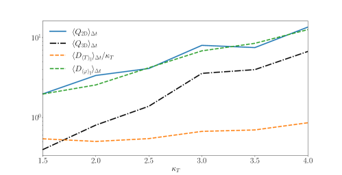
Figure 21: Plot of the time-averaged 2D heat flux $Q_{\text{2D}}$ given by eq. 144 (solid blue), the 3D heat flux $Q_{\text{3D}}\equiv Q-Q_{\text{2D}}$ (dash-dotted black), the collisional dissipation in eq. 142 $D_{\mathopen{}\mathclose{{}\left\langle\varphi}\right\rangle_{\parallel}}$ given by eq. 145 (dashed green), and the collisional dissipation in eq. 143, $D_{\mathopen{}\mathclose{{}\left\langle T}\right\rangle_{\parallel}}/\kappa_{T}$ given by eq. 146 (dashed orange) versus $\kappa_{T}$ for $\chi=0.05$, $L_{x}=L_{y}=60$ and $L_{\parallel}=0.5$. We see that $Q_{\text{2D}}$ is more than twice $Q_{\text{3D}}$, and is balanced nearly perfectly by $D_{\mathopen{}\mathclose{{}\left\langle\varphi}\right\rangle_{\parallel}}$, i.e., the nonlinear transfer in eq. 58 is small. On the other hand, $D_{\mathopen{}\mathclose{{}\left\langle T}\right\rangle_{\parallel}}/\kappa_{T}Q_{\text{2D}}\ll 1$, so the majority of energy injected into $\mathopen{}\mathclose{{}\left\langle T}\right\rangle_{\parallel}$ is nonlinearly transferred to 3D modes.

Appendix G Kinetic slab-ITG instability

The results in section 4.3.2 rely on the existence of the collisionless sITG instability at short parallel and perpendicular wavelengths $k_{\parallel}\sim\kappa_{T}k_{\perp}^{2}\gg 1$. However, the existence of a collisionless sITG instability at infinitely short perpendicular scales is a more general fact that can be established without resorting to a fluid limit. To show this, let us find the sITG dispersion relation directly from the collisionless kinetic equation.

We begin at appendix A with zero collisionality ($\nu_{i}=0$), no magnetic curvature ($L_{B}^{-1}=0$), and linearised:

$$\frac{\partial}{\partial t}\mathopen{}\mathclose{{}\left(h-\mathopen{}\mathclose{{}\left\langle\varphi}\right\rangle_{\boldsymbol{R}}F_{i}}\right)+{v_{\parallel}}\partial_{\parallel}h+\frac{\rho_{i}v_{\text{th}i}}{2L_{T}}\mathopen{}\mathclose{{}\left(\frac{v^{2}}{v^{2}_{ti}}-\frac{3}{2}}\right)F_{i}\frac{\partial\mathopen{}\mathclose{{}\left\langle\varphi}\right\rangle_{\boldsymbol{R}}}{\partial Y}=0.$$ (149)

We shall consider Fourier modes $h,\varphi\propto\exp\mathopen{}\mathclose{{}\left(-i\omega_{\boldsymbol{k}}t+i{\boldsymbol{k}}\bcdot{\boldsymbol{r}}}\right)$. Rearranging eq. 149 and using the fact that $F_{i}$ is a Maxwellian with density $n_{i}$ and thermal speed $v_{\text{th}i}$, we find

$$\frac{h_{\boldsymbol{k}}}{\varphi_{\boldsymbol{k}}}=\frac{n_{i}}{\pi^{3/2}v_{\text{th}i}^{3}}\frac{\zeta+\zeta_{*}\mathopen{}\mathclose{{}\left(\hat{v}^{2}-\frac{3}{2}}\right)}{\zeta-\text{sgn}\mathopen{}\mathclose{{}\left(k_{\parallel}}\right)\hat{v}_{\parallel}}e^{-\hat{v}^{2}}J_{0}\mathopen{}\mathclose{{}\left(k_{\perp}\rho_{i}\hat{v}_{\perp}}\right),$$ (150)

where $\zeta\equiv\omega_{\boldsymbol{k}}/|k_{\parallel}|v_{\text{th}i}$, $\zeta_{*}\equiv\rho_{i}v_{\text{th}i}k_{y}/2L_{T}|k_{\parallel}|v_{\text{th}i}$, $\hat{{\boldsymbol{v}}}\equiv{\boldsymbol{v}}/v_{\text{th}i}$, $\text{sgn}(k_{\parallel})\equiv k_{\parallel}/|k_{\parallel}|$, and $J_{0}$ is the zeroth-order Bessel function of the first kind. Substituting eq. 150 into the quasineutrality condition eq. 88, we find

$$1+\tau =\frac{1}{n_{i}}\int d^{3}{\boldsymbol{v}}\ J_{0}\mathopen{}\mathclose{{}\left(k_{\perp}\rho_{i}\hat{v}_{\perp}}\right)\frac{h_{\boldsymbol{k}}}{\varphi_{\boldsymbol{k}}}$$

$$=\frac{1}{\sqrt{\pi}}\int_{-\infty}^{+\infty}d\hat{v}_{\parallel}\ e^{-\hat{v}_{\parallel}^{2}}\int_{0}^{+\infty}d(\hat{v}_{\perp}^{2})e^{-\hat{v}_{\perp}^{2}}\frac{\zeta+\zeta_{*}\mathopen{}\mathclose{{}\left(\hat{v}^{2}-\frac{3}{2}}\right)}{\zeta-\hat{v}_{\parallel}}J_{0}^{2}\mathopen{}\mathclose{{}\left(k_{\perp}\rho_{i}\hat{v}_{\perp}}\right),$$ (151)

where $\text{sgn}\mathopen{}\mathclose{{}\left(k_{\parallel}}\right)$ is absorbed into $\hat{v}_{\parallel}$ and the integral over $\hat{v}_{\parallel}$ is taken along the Landau contour (i.e., below the pole). After performing the integrals in appendix G, we find the sITG dispersion relation:

$$\mathopen{}\mathclose{{}\left\{-\mathopen{}\mathclose{{}\left(\zeta-\frac{1}{2}\zeta_{*}}\right)\Gamma_{0}(\alpha)+\zeta_{*}\alpha\Gamma_{1}(\alpha)}\right\}Z(\zeta)-\zeta_{*}\zeta\Gamma_{0}(\alpha)\mathopen{}\mathclose{{}\left[1+\zeta Z(\zeta)}\right]=1+\tau,$$ (152)

where $\alpha\equiv k_{\perp}^{2}\rho_{i}^{2}/2$, $\Gamma_{0}(\alpha)\equiv I_{0}(\alpha)e^{-\alpha}$, $\Gamma_{1}(\alpha)\equiv\mathopen{}\mathclose{{}\left[I_{0}(\alpha)-I_{1}(\alpha)}\right]e^{-\alpha}$, $I_{0}(\alpha)$ and $I_{1}(\alpha)$ are the zeroth- and first-order modified Bessel functions of the first kind, and

$$Z(\zeta)=\frac{1}{\sqrt{\pi}}\int dz\frac{e^{-z^{2}}}{z-\zeta}$$ (153)

is the plasma dispersion function (Fried & Conte, 1961), with the integral taken along the Landau contour. To express the relevant integral moments of $J_{0}^{2}$, we used the relation

$$\int_{0}^{+\infty}d(x^{2})\ J_{m}(bx)J_{n}(cx)e^{-x^{2}/a}=aI_{0}\mathopen{}\mathclose{{}\left(a\frac{b^{2}+c^{2}}{4}}\right)e^{-abc/2}\delta_{mn},$$ (154)

for $a=1$ and $b=c=k_{\perp}\rho_{i}$ (Watson, 1966, p. 395).

We can verify that the ‘fluid’ dispersion relation eq. 31 is an asymptotic limit of eq. 152 by expanding the latter for the ordering in eq. 3. Under this ordering, $\zeta\sim\zeta_{*}\sim 1/\sqrt{\tau}\sim 1/\sqrt{\alpha}\gg 1$. The large-$\zeta$ and small-$\alpha$ expansions of the plasma dispersion function and the Bessel functions are

$$Z(\zeta)\approx-\frac{1}{\zeta}\mathopen{}\mathclose{{}\left(1+\frac{1}{2\zeta^{2}}}\right),\quad\Gamma_{0}(\alpha)=1-\alpha+\mathcal{O}\mathopen{}\mathclose{{}\left(\alpha^{2}}\right),\quad\Gamma_{1}(\alpha)=1+\mathcal{O}\mathopen{}\mathclose{{}\left(\alpha}\right).$$ (155)

Using these along with $\alpha/\tau=k_{\perp}^{2}\rho_{s}^{2}$, and adopting the normalisations eq. 10, we find that eq. 152 reduces to eq. 31.

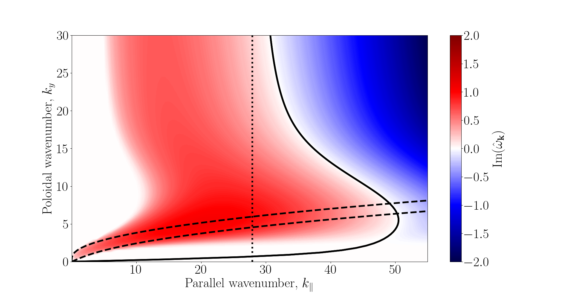
Figure 22: The linear growth rate ${\text{Im}{(\omega_{\boldsymbol{k}})}}$ of the kinetic dispersion relation eq. 152 for $\tau=0.01$, normalised as $\hat{\omega}_{\boldsymbol{k}}=L_{T}\omega_{\boldsymbol{k}}/c_{s}\tau$, which is equivalent to normalisation of time in eq. 10 for $\kappa_{T}=1$. The wavenumbers $k_{y}$ and $k_{\parallel}$ are also normalised according to eq. 10 with $\kappa_{T}=1$. The largest kinetic growth rate is ${\text{Im}{(\hat{\omega}_{\boldsymbol{k}}^{\text{kin}})}}\approx 1.07$, while the largest cold-ion growth rate, given by eq. 44, is ${\text{Im}{(\hat{\omega}_{\boldsymbol{k}}^{\text{cold}})}}\approx 0.71$. The vertical dotted line is the critical parallel wavenumber $k_{\parallel}^{(c)}$ for $k_{\perp}\gg 1$ kinetic modes eq. 159. The dashed black lines are the cold-ion stability boundary eq. 33. The solid black line is the kinetic stability boundary eq. 158. The kinetic sITG instability has a finite growth rate at $k_{\perp}\to\infty$.

We can also find the general stability boundary of eq. 152 in the standard way, by looking for the parameters that allow a ${\text{Im}{(\zeta)}}=0$ solution. For such a solution, the only imaginary contributions to eq. 152 come from the terms containing the plasma dispersion function, so the coefficient of $Z(\zeta)$ must be zero. This gives us a system of two equations:

$$(1+\tau)+\zeta\zeta_{*}\Gamma_{0}(\alpha)=0,$$ (156)

$$\mathopen{}\mathclose{{}\left(\zeta-\frac{1}{2}\zeta_{*}}\right)\Gamma_{0}(\alpha)-\zeta_{*}\alpha\Gamma_{1}(\alpha)+\zeta^{2}\zeta_{*}\Gamma_{0}(\alpha)=0.$$ (157)

Solving this, we find

$$\zeta_{*}^{2}=\frac{2(1+\tau)\mathopen{}\mathclose{{}\left[1+\tau-\Gamma_{0}(\alpha)}\right]}{\Gamma_{0}^{2}(\alpha)+2\alpha\Gamma_{0}(\alpha)\Gamma_{1}(\alpha)}.$$ (158)

Using $\omega_{*}\equiv\rho_{i}v_{\text{th}i}k_{y}/2L_{T}$ and eq. 10, we can express $\zeta_{*}$ and $\alpha$ in terms of the normalised $\hat{k}_{x}$, $\hat{k}_{y}$, and $\hat{k}_{\parallel}$. This gives us an analytic expression for the stability boundary. In the limit $k_{\perp}\gg 1$, i.e., $\alpha\gg 1$, we can expand eq. 158 to find that an instability exists for

$$k_{\parallel}<\frac{1}{2\sqrt{\pi}(1+\tau)L_{T}}\equiv k_{\parallel}^{(c)}.$$ (159)

Similarly to the parallel wavenumber at which Braginskii viscosity would kick in (see section 4.3.2), $k_{\parallel}^{(c)}$ exists outside of the cold-ion ordering for our model, as it is asymptotically large in the ordering eq. 3: $k_{\parallel}^{(c)}L_{B}\sim\mathcal{O}(L_{B}/L_{T})\sim\mathcal{O}(\tau^{-1})\gg 1$. Figure 22 shows the growth rate obtained from solving eq. 152 numerically, along with the stability boundary of the cold-ion limit eq. 33.

Appendix H Quasilinear ZF stress of kinetic sITG modes

The stability of the zonal staircase in the 3D system eq. 11–eq. 13 was attributed to the turbulent stress in the presence of strong zonal shear (see section 4.2.5, as well as Ivanov et al., 2020). In the fluid limit, this stress was found to be the sum of Reynolds and diamagnetic stresses. Therefore, we were able to conclude that whether a mode with wavenumber ${\boldsymbol{q}}$ feeds or destroys the ZFs depends on the sign of the quantity $1+{\text{Re}{(T_{\boldsymbol{q}}/\varphi_{\boldsymbol{q}})}}$ (see section 4.1). We then found that we could predict the Dimits threshold by investigating the value of this quantity for the fastest-growing linear ITG modes. Here we generalise this approach to kinetic sITG modes.

We start with the ion GK equation appendix A and the quasineutrality condition eq. 88. We shall ignore the influence of collisions, so drop the collision operator on the right-hand side of appendix A. Taking a $(1/n_{i})\int d^{3}{\boldsymbol{v}}$ moment of appendix A at constant ${\boldsymbol{r}}$ and integrating over a flux surface, we find

$$\partial_{t}(\overline{\varphi-\mathopen{}\mathclose{{}\left\langle\mathopen{}\mathclose{{}\left\langle\varphi}\right\rangle_{\boldsymbol{R}}}\right\rangle_{\boldsymbol{r}}})+\frac{\rho_{i}v_{\text{th}i}}{2n_{i}}\int d^{3}{\boldsymbol{v}}\ \overline{\mathopen{}\mathclose{{}\left\langle\mathopen{}\mathclose{{}\left\{\mathopen{}\mathclose{{}\left\langle\varphi}\right\rangle_{\boldsymbol{R}},h}\right\}}\right\rangle_{\boldsymbol{r}}}=0.$$ (160)

With $\varphi$ and $h$ decomposed into Fourier modes, $\varphi_{\boldsymbol{k}},h_{\boldsymbol{k}}\propto\exp\mathopen{}\mathclose{{}\left(i{\boldsymbol{k}}\bcdot{\boldsymbol{r}}}\right)$, eq. 160 gives the following equation for each mode:

$$\partial_{t}\mathopen{}\mathclose{{}\left[1-\Gamma_{0}(\alpha)}\right]\varphi_{\boldsymbol{k}}+\frac{\rho_{i}v_{\text{th}i}}{2n_{i}}\int d^{3}{\boldsymbol{v}}\ J_{0}\mathopen{}\mathclose{{}\left(k\rho_{i}\hat{v}_{\perp}}\right)\sum_{\boldsymbol{q}}\hat{{\boldsymbol{z}}}\bcdot({\boldsymbol{q}}_{\perp}\times{\boldsymbol{k}})J_{0}\mathopen{}\mathclose{{}\left(|{\boldsymbol{q}}_{\perp}-{\boldsymbol{k}}|\rho_{i}\hat{v}_{\perp}}\right)\varphi_{{\boldsymbol{k}}-{\boldsymbol{q}}}h_{\boldsymbol{q}}=0,$$ (161)

where ${\boldsymbol{k}}$ is a zonal wavenumber, i.e., ${\boldsymbol{k}}=k\hat{{\boldsymbol{x}}}$, $\alpha=k^{2}\rho_{i}^{2}/2$, and the rest of the notation is the same as in appendix G. To make progress, let us assume that the scale of the ZF is much larger than the scale of the modes that contribute to the nonlinear term in eq. 161, i.e., that $k\rho_{i}\ll q_{\perp}\rho_{i}\sim 1$. We can then expand

$$|{\boldsymbol{q}}_{\perp}-{\boldsymbol{k}}|=\sqrt{({\boldsymbol{q}}_{\perp}-{\boldsymbol{k}})^{2}}=q_{\perp}\mathopen{}\mathclose{{}\left[1-\frac{{\boldsymbol{k}}\bcdot{\boldsymbol{q}}_{\perp}}{q_{\perp}^{2}}+\mathcal{O}\mathopen{}\mathclose{{}\left(k^{2}\rho_{i}^{2}}\right)}\right],$$ (162)

whence

$$J_{0}\mathopen{}\mathclose{{}\left(|{\boldsymbol{q}}_{\perp}-{\boldsymbol{k}}|\rho_{i}\hat{v}_{\perp}}\right)=J_{0}\mathopen{}\mathclose{{}\left(q_{\perp}\rho_{i}\hat{v}_{\perp}}\right)+q_{\perp}\rho_{i}\hat{v}_{\perp}\frac{{\boldsymbol{k}}\bcdot{\boldsymbol{q}}_{\perp}}{q_{\perp}^{2}}J_{1}\mathopen{}\mathclose{{}\left(q_{\perp}\rho_{i}\hat{v}_{\perp}}\right)+\mathcal{O}\mathopen{}\mathclose{{}\left(k^{2}\rho_{i}^{2}}\right),$$ (163)

$$J_{0}\mathopen{}\mathclose{{}\left(k_{\perp}\rho_{i}\hat{v}_{\perp}}\right)=1+\mathcal{O}\mathopen{}\mathclose{{}\left(k^{2}\rho_{i}^{2}}\right),$$ (164)

$$1-\Gamma_{0}(\alpha)=\frac{1}{2}k^{2}\rho_{i}^{2}+\mathcal{O}\mathopen{}\mathclose{{}\left(k^{4}\rho_{i}^{4}}\right).$$ (165)

The integral in eq. 161 vanishes to the lowest order in $k\rho_{i}$, viz.,

$$\int d^{3}{\boldsymbol{v}}\ \sum_{\boldsymbol{q}}\hat{{\boldsymbol{z}}}\bcdot({\boldsymbol{q}}_{\perp}\times{\boldsymbol{k}})J_{0}\mathopen{}\mathclose{{}\left(q_{\perp}\rho_{i}\hat{v}_{\perp}}\right)\varphi_{{\boldsymbol{k}}-{\boldsymbol{q}}}h_{\boldsymbol{q}}=\int d^{3}{\boldsymbol{v}}\ \mathopen{}\mathclose{{}\left\{\varphi,\mathopen{}\mathclose{{}\left\langle h}\right\rangle_{\boldsymbol{r}}}\right\}_{\boldsymbol{k}}=n_{i}(1+\tau)\mathopen{}\mathclose{{}\left\{\varphi,\varphi}\right\}_{\boldsymbol{k}}=0$$ (166)

by quasineutrality eq. 88. To the next order in $k\rho_{i}$, eq. 161 becomes

$$\frac{1}{2}k^{2}\rho_{i}^{2}\partial_{t}\varphi_{\boldsymbol{k}}+\frac{1}{4}\rho_{i}^{3}v_{\text{th}i}\sum_{\boldsymbol{q}}\hat{{\boldsymbol{z}}}\bcdot({\boldsymbol{q}}_{\perp}\times{\boldsymbol{k}}){\boldsymbol{k}}\bcdot{\boldsymbol{q}}_{\perp}\varphi_{{\boldsymbol{k}}-{\boldsymbol{q}}}\mathcal{P}_{\boldsymbol{q}}=0,$$ (167)

where we have defined the GK perpendicular pressure perturbation

$$\mathcal{P}_{\boldsymbol{q}}\equiv\frac{1}{n_{i}}\int d^{3}{\boldsymbol{v}}\ \hat{v}_{\perp}^{2}\frac{2J_{1}\mathopen{}\mathclose{{}\left(q_{\perp}\rho_{i}\hat{v}_{\perp}}\right)}{q_{\perp}\rho_{i}\hat{v}_{\perp}}h_{\boldsymbol{q}}.$$ (168)

Note that for $q_{\perp}\rho_{i}\ll 1$, $J_{1}\mathopen{}\mathclose{{}\left(q_{\perp}\rho_{i}\hat{v}_{\perp}}\right)\approx q_{\perp}\rho_{i}\hat{v}_{\perp}/2$, and eq. 168 gives

$$\mathcal{P}_{\boldsymbol{q}}\approx\frac{1}{n_{i}}\int d^{3}{\boldsymbol{v}}\ \hat{v}_{\perp}^{2}h_{\boldsymbol{q}}=p_{\boldsymbol{q}},$$ (169)

where $p_{\boldsymbol{q}}$ is the pressure perturbation in the cold-ion model.

Fourier transforming eq. 167 back to real space, we find

$$\partial_{t}\overline{\varphi}+\frac{1}{2}\rho_{i}v_{\text{th}i}\overline{\partial_{x}\mathcal{P}\partial_{y}\varphi}=0.$$ (170)

Therefore, $\overline{\partial_{x}\mathcal{P}\partial_{y}\varphi}$ is the GK version of the turbulent stress $\Pi_{t}$ (see section 4.1.1) for large-scale ZFs, but $\rho_{i}$-scale turbulence. In the limit of large-scale turbulence ($q_{\perp}\rho_{i}\ll 1$), eq. 170 reduces to

$$\partial_{t}\overline{\varphi}+\frac{1}{2}\rho_{i}v_{\text{th}i}\overline{\partial_{x}p\partial_{y}\varphi}=0.$$ (171)

Note that eq. 171 is not the same as eq. 53 with $\Pi_{\chi}=0$. This is expected because eq. 53 was obtained in the limit $k_{\perp}\rho_{i}\sim q_{\perp}\rho_{i}\ll 1$, where ${\boldsymbol{k}}$ and ${\boldsymbol{q}}$ were the typical wavenumbers of zonal and nonzonal modes, respectively. In contrast, taking $q_{\perp}\rho_{i}\ll 1$ in eq. 170 is actually the limit $k_{\perp}\rho_{i}\ll q_{\perp}\rho_{i}\ll 1$. The difference between eq. 53 and eq. 171 is an exact derivative, viz., $\partial_{x}(\overline{\varphi\partial_{y}p})$, and so does not influence the integrated momentum transport in a shear zone of radial width $d$:

$$\frac{1}{d}\int dx\overline{\partial_{x}\mathcal{P}\partial_{y}\varphi}=-\sum_{\boldsymbol{q}}q_{x}q_{y}|\varphi_{\boldsymbol{q}}|^{2}{\text{Re}{\mathopen{}\mathclose{{}\left(\frac{\mathcal{P}_{\boldsymbol{q}}}{\varphi_{\boldsymbol{q}}}}\right)}},$$ (172)

where the correspondence with eq. 55 is evident. Therefore, following the arguments in section 4.1.1 and (Ivanov et al., 2020), we can conclude that the effect on the ZFs of a mode with wavenumber ${\boldsymbol{q}}$ depends on the sign of ${\text{Re}{(\mathcal{P}_{\boldsymbol{q}}/\varphi_{\boldsymbol{q}})}}$, viz., modes with ${\text{Re}{(\mathcal{P}_{\boldsymbol{q}}/\varphi_{\boldsymbol{q}}>0)}}$ feed momentum into the ZFs, while those with ${\text{Re}{(\mathcal{P}_{\boldsymbol{q}}/\varphi_{\boldsymbol{q}})}}<0$ take momentum away from the ZFs.

Let us calculate ${\text{Re}{(\mathcal{P}_{\boldsymbol{q}}/\varphi_{\boldsymbol{q}})}}$ for the kinetic sITG modes that we found in appendix G. From eq. 168, we find

$$\frac{\mathcal{P}_{\boldsymbol{q}}}{\varphi_{\boldsymbol{q}}} =\frac{2}{n_{i}}\int d^{3}{\boldsymbol{v}}\frac{\hat{v}_{\perp}}{q_{\perp}\rho_{i}}J_{1}\mathopen{}\mathclose{{}\left(q_{\perp}\rho_{i}\hat{v}_{\perp}}\right)$$

$$=\frac{1}{\sqrt{\pi}}\int_{-\infty}^{+\infty}d\hat{v}_{\parallel}\ e^{-\hat{v}_{\parallel}^{2}}\int_{0}^{+\infty}d(\hat{v}_{\perp}^{2})e^{-\hat{v}_{\perp}^{2}}\frac{\zeta+\zeta_{*}\mathopen{}\mathclose{{}\left(\hat{v}^{2}-\frac{3}{2}}\right)}{\zeta-\hat{v}_{\parallel}}\frac{2\hat{v}_{\perp}}{q_{\perp}\rho_{i}}J_{1}\mathopen{}\mathclose{{}\left(q_{\perp}\rho_{i}\hat{v}_{\perp}}\right)J_{0}\mathopen{}\mathclose{{}\left(q_{\perp}\rho_{i}\hat{v}_{\perp}}\right),$$ (173)

where we have substituted the linear GK expression eq. 150 for $h$, $\hat{{\boldsymbol{v}}}={\boldsymbol{v}}/v_{\text{th}i}$, and $\zeta$ and $\zeta_{*}$ are defined equivalently to those after eq. 150, but with ${\boldsymbol{k}}$ replaced by ${\boldsymbol{q}}$. Notice that

$$\frac{2\hat{v}_{\perp}}{q_{\perp}\rho_{i}}J_{1}\mathopen{}\mathclose{{}\left(q_{\perp}\rho_{i}\hat{v}_{\perp}}\right)J_{0}\mathopen{}\mathclose{{}\left(q_{\perp}\rho_{i}\hat{v}_{\perp}}\right)=-\frac{1}{q_{\perp}\rho_{i}}\frac{\partial}{\partial(q_{\perp}\rho_{i})}J_{0}^{2}\mathopen{}\mathclose{{}\left(q_{\perp}\rho_{i}\hat{v}_{\perp}}\right)=-\frac{\partial}{\partial\alpha}J_{0}^{2}\mathopen{}\mathclose{{}\left(q_{\perp}\rho_{i}\hat{v}_{\perp}}\right),$$ (174)

where $\alpha=q_{\perp}^{2}\rho_{i}^{2}/2$. Therefore, appendix H can be written as

$$\frac{\mathcal{P}_{\boldsymbol{q}}}{\varphi_{\boldsymbol{q}}}=-\frac{\partial}{\partial\alpha}\frac{1}{\sqrt{\pi}}\int_{-\infty}^{+\infty}d\hat{v}_{\parallel}\ e^{-\hat{v}_{\parallel}^{2}}\int_{0}^{+\infty}d(\hat{v}_{\perp}^{2})e^{-\hat{v}_{\perp}^{2}}\frac{\zeta+\zeta_{*}\mathopen{}\mathclose{{}\left(\hat{v}^{2}-\frac{3}{2}}\right)}{\zeta-\hat{v}_{\parallel}}J_{0}^{2}\mathopen{}\mathclose{{}\left(q_{\perp}\rho_{i}\hat{v}_{\perp}}\right),$$ (175)

where the partial derivative with respect to $\alpha$ is taken at constant $\zeta_{*}$. We have already calculated the expression in eq. 175 that needs to be differentiated — this is precisely the left-hand side of eq. 152. Taking the derivative, we obtain

$$\frac{\mathcal{P}_{\boldsymbol{q}}}{\varphi_{\boldsymbol{q}}}=\mathopen{}\mathclose{{}\left[-\mathopen{}\mathclose{{}\left(\zeta-\frac{1}{2}\zeta_{*}}\right)\Gamma_{1}(\alpha)-\zeta_{*}\Gamma_{0}(\alpha)+2\zeta_{*}\alpha\Gamma_{1}(\alpha)}\right]Z(\zeta)-\zeta\zeta_{*}\Gamma_{1}(\alpha)\mathopen{}\mathclose{{}\left[1+\zeta Z(\zeta)}\right].$$ (176)

We determine ${\text{Re}{(\mathcal{P}_{\boldsymbol{q}}/\varphi_{\boldsymbol{q}})}}$ for the sITG modes by solving for $\zeta$ using the dispersion relation eq. 152 and then substituting for $\zeta$ into eq. 176. As we can see in figures 23 and 24, both for $\tau\ll 1$ and $\tau\sim 1$, the small-scale sITG instability drives the ZFs. The role of the dominant sITG modes (i.e., those with the largest growth rate) in the cold-ion limit is clear — they support the ZFs, just as they do in the fluid model. However, as $\tau$ approaches $1$, it is difficult to discern their effect on the ZFs without the knowledge of the spectrum of the fluctuation amplitudes at the relevant wavenumbers. However, it appears that the number of ZF-destabilising modes increases with increasing $\tau$. This suggests that the Dimits threshold might be sensitive to the value of $\tau$.

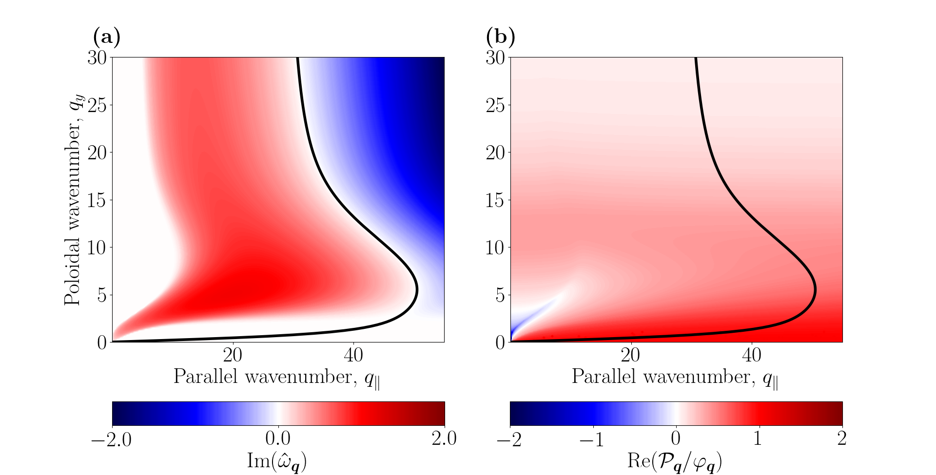
Figure 23: (a) Growth rate ${\text{Im}{(\hat{\omega}_{\boldsymbol{q}})}}$, normalised as $\hat{\omega}_{\boldsymbol{q}}=L_{T}\omega_{\boldsymbol{q}}/c_{s}\tau$, which is equivalent to normalisation of time in eq. 10 for $\kappa_{T}=1$. (b) The ratio ${\text{Re}{(\mathcal{P}_{\boldsymbol{q}}/\varphi_{\boldsymbol{q}})}}$, given by eq. 176. For both panels, $\tau=0.01$ and $q_{x}=0$. The wavenumbers $q_{y}$ and $q_{\parallel}$ are also normalised according to eq. 10 with $\kappa_{T}=1$. The solid black lines show the kinetic stability boundary eq. 158. It is evident that the vast majority of sITG modes, including the dominant ones, support the ZFs, i.e., satisfy ${\text{Re}{(\mathcal{P}_{\boldsymbol{q}}/\varphi_{\boldsymbol{q}})}}>0$.

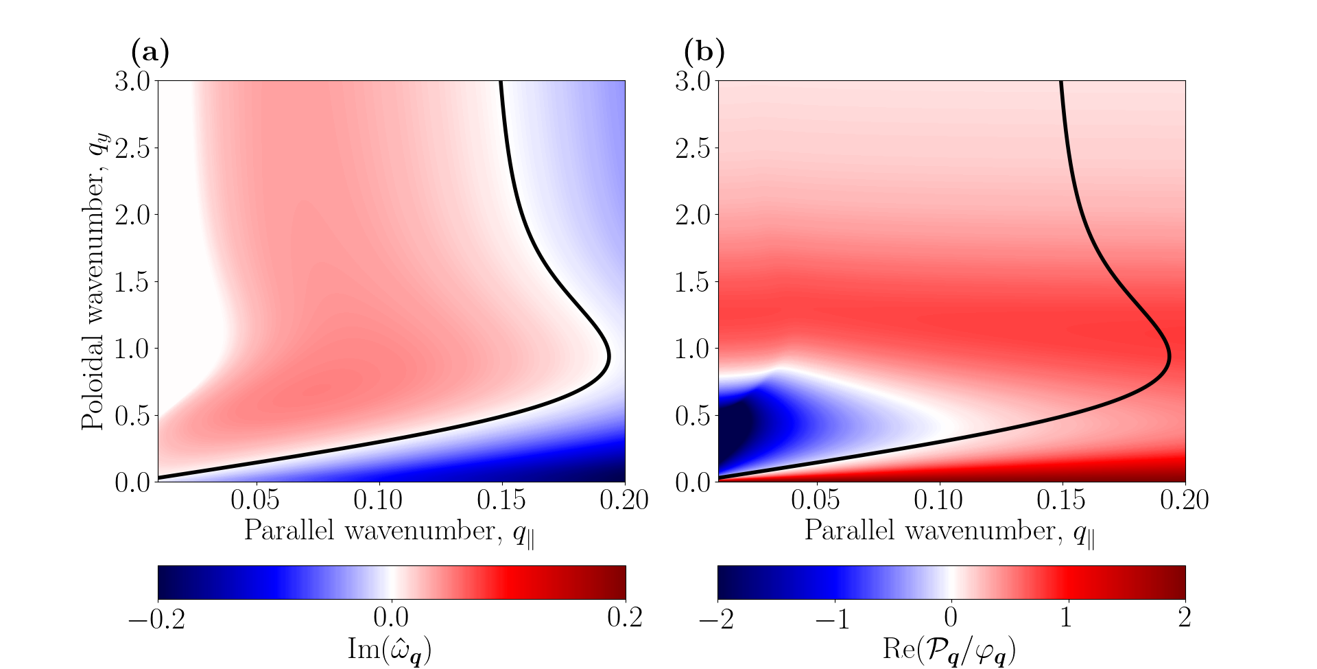
Figure 24: Same as fig. 23, but for $\tau=1$. Evidently, the small-scale sITG modes at $q_{y}\gg 1$ have ${\text{Re}{(\mathcal{P}_{\boldsymbol{q}}/\varphi_{\boldsymbol{q}})}}>0$, i.e., they support the ZFs. However, it is no longer obvious whether the dominant sITG modes support or destroy the ZFs.

References

- Barnes et al. (2011) Barnes, M, Parra, FI & Schekochihin, AA 2011 Critically balanced ion temperature gradient turbulence in fusion plasmas. Phys. Rev. Lett. 107, 115003.
- Braginskii (1965) Braginskii, SI 1965 Transport processes in a plasma. Reviews of Plasma Physics 1, 205.
- Coppi et al. (1967) Coppi, B, Rosenbluth, MN & Sagdeev, RZ 1967 Instabilities due to temperature gradients in complex magnetic field configurations. Phys. Fluids 10, 582.
- Cowley et al. (1991) Cowley, SC, Kulsrud, RM & Sudan, R 1991 Considerations of ion-temperature-gradient-driven turbulence. Phys. Fluids B 3, 2767.
- Diamond et al. (2005) Diamond, PH, Itoh, S-I, Itoh, K & Hahm, TS 2005 Zonal flows in plasma—a review. Plasma Phys. Control. Fusion 47, R35.
- Dif-Pradalier et al. (2010) Dif-Pradalier, G, Diamond, PH, Grandgirard, V, Sarazin, Y, Abiteboul, J, Garbet, X, Ghendrih, Ph, Strugarek, A, Ku, S & Chang, CS 2010 On the validity of the local diffusive paradigm in turbulent plasma transport. Phys. Rev. E 82, 025401.
- Dif-Pradalier et al. (2017) Dif-Pradalier, G, Hornung, G, Garbet, X, Ghendrih, Ph, Grandgirard, V, Latu, G & Sarazin, Y 2017 The ExB staircase of magnetised plasmas. Nuclear Fusion 57, 066026.
- Dorland & Hammett (1993) Dorland, W & Hammett, GW 1993 Gyrofluid turbulence models with kinetic effects. Phys. Fluids B 5, 812.
- Dorland et al. (2000) Dorland, W, Jenko, F, Kotschenreuther, M & Rogers, BN 2000 Electron temperature gradient turbulence. Phys. Rev. Lett. 85, 5579.
- Drake et al. (1988) Drake, JF, Guzdar, PN & Hassam, AB 1988 Streamer formation in plasma with a temperature gradient. Phys. Rev. Lett. 61, 2205.
- Fox et al. (2017) Fox, MFJ, van Wyk, F, Field, AR, Ghim, Y-c, Parra, FI, Schekochihin, AA & Team, MAST 2017 Symmetry breaking in MAST plasma turbulence due to toroidal flow shear. Plasma Phys. Control. Fusion 59, 034002.
- Frei et al. (2022) Frei, BJ, Hoffmann, ACD & Ricci, P 2022 Local gyrokinetic collisional theory of the ion-temperature gradient mode. J. Plasma Phys. 88, 905880304.
- Fried & Conte (1961) Fried, BD & Conte, SD 1961 The Plasma Dispersion Function. Academic Press.
- Guzdar et al. (1983) Guzdar, PN, Chen, L, Tang, WM & Rutherford, PH 1983 Ion-temperature-gradient instability in toroidal plasmas. Phys. Fluids 26, 673.
- Hallenbert & Plunk (2021) Hallenbert, A & Plunk, GG 2021 Predicting the dimits shift through reduced mode tertiary instability analysis in a strongly driven gyrokinetic fluid limit. J. Plasma Phys. 87, 905870508.
- Hammett et al. (1993) Hammett, GW, Beer, MA, Dorland, W, Cowley, SC & Smith, SA 1993 Developments in the gyrofluid approach to tokamak turbulence simulations. Plasma Phys. Control. Fusion 35, 973.
- Ivanov et al. (2020) Ivanov, PG, Schekochihin, AA, Dorland, W, Field, AR & Parra, FI 2020 Zonally dominated dynamics and Dimits threshold in curvature-driven ITG turbulence. J. Plasma Phys. 86, 855860502.
- Kinsey et al. (2006) Kinsey, JE, Waltz, RE & Candy, J 2006 The effect of safety factor and magnetic shear on turbulent transport in nonlinear gyrokinetic simulations. Physics of Plasmas 13, 022305.
- Kobayashi & Rogers (2012) Kobayashi, S & Rogers, BN 2012 The quench rule, Dimits shift, and eigenmode localization by small-scale zonal flows. Phys. Plasmas 19, 012315.
- Kotschenreuther et al. (1995) Kotschenreuther, M, Rewoldt, G & Tang, WM 1995 Comparison of initial value and eigenvalue codes for kinetic toroidal plasma instabilities. Comput. Phys. Commun. 88, 128.
- Newton et al. (2010) Newton, SL, Cowley, SC & Loureiro, NF 2010 Understanding the effect of sheared flow on microinstabilities. Plasma Phys. Control. Fusion 52, 125001.
- Parra et al. (2011) Parra, FI, Barnes, M & Peeters, AG 2011 Up-down symmetry of the turbulent transport of toroidal angular momentum in tokamaks. Phys. Plasmas 18, 062501.
- Pogutse (1968) Pogutse, OP 1968 Magnetic drift instability in a collisionless plasma. Plasma Physics 10, 649.
- Rath et al. (2016) Rath, F, Peeters, AG, Buchholz, R, Grosshauser, SR, Migliano, P, Weikl, A & Strintzi, D 2016 Comparison of gradient and flux driven gyro-kinetic turbulent transport. Phys. Plasmas 23, 052309.
- Rath & Sridhar (1992) Rath, S & Sridhar, S 1992 Core instability of elliptic drift vortices. Phys. Fluids B 4, 1367.
- Ricci et al. (2006) Ricci, P, Rogers, BN & Dorland, W 2006 Small-scale turbulence in a closed-field-line geometry. Phys. Rev. Lett. 97, 245001.
- Rogers et al. (2000) Rogers, BN, Dorland, W & Kotschenreuther, M 2000 Generation and stability of zonal flows in ion-temperature-gradient mode turbulence. Phys. Rev. Lett. 85, 5336.
- Rudakov & Sagdeev (1961) Rudakov, LI & Sagdeev, RZ 1961 On the instability of a nonuniform rarefied plasma in a strong magnetic field. Dokl. Akad. Nauk SSSR 138, 581.
- Schekochihin et al. (2009) Schekochihin, AA, Cowley, SC, Dorland, W, Hammett, GW, Howes, GG, Quataert, E & Tatsuno, T 2009 Astrophysical gyrokinetics: kinetic and fluid turbulent cascades in magnetized weakly collisional plasmas. Astrophys. J. Suppl. S. 182, 310.
- Smolyakov et al. (2002) Smolyakov, AI, Yagi, M & Kishimoto, Y 2002 Short wavelength temperature gradient driven modes in tokamak plasmas. Phys. Rev. Lett. 89, 125005.
- St-Onge (2017) St-Onge, DA 2017 On non-local energy transfer via zonal flow in the Dimits shift. J. Plasma Phys. 83, 905830504.
- Villard et al. (2013) Villard, L, Angelino, P, Bottino, A, Brunner, S, Jolliet, S, McMillan, BF, Tran, TM & Vernay, T 2013 Global gyrokinetic ion temperature gradient turbulence simulations of ITER. Plasma Phys. Control. Fusion 55, 074017.
- Watson (1966) Watson, GN 1966 A Treatise on the theory of Bessel functions, 2nd edn. CUP.
- van Wyk et al. (2017) van Wyk, F, Highcock, EG, Field, AR, Roach, CM, Schekochihin, AA, Parra, FI & Dorland, W 2017 Ion-scale turbulence in MAST: anomalous transport, subcritical transitions, and comparison to BES measurements. Plasma Phys. Control. Fusion 59, 114003.
- van Wyk et al. (2016) van Wyk, F, Highcock, EG, Schekochihin, AA, Roach, CM, Field, AR & Dorland, W 2016 Transition to subcritical turbulence in a tokamak plasma. J. Plasma Phys. 82, 905820609.
- Zhu et al. (2018) Zhu, H, Zhou, Y & Dodin, IY 2018 On the Rayleigh–Kuo criterion for the tertiary instability of zonal flows. Phys. Plasmas 25, 082121.
- Zhu et al. (2020a) Zhu, H, Zhou, Y & Dodin, IY 2020a Theory of the tertiary instability and the Dimits shift from reduced drift-wave models. Phys. Rev. Lett. 124, 055002.
- Zhu et al. (2020b) Zhu, H, Zhou, Y & Dodin, IY 2020b Theory of the tertiary instability and the dimits shift within a scalar model. J. Plasma Phys. 86, 905860405.