Multi-level images around Kerr-Newman black holes

Abstract

We study the lensing effects of Kerr-Newman (KN) black holes and the multi-level images of luminous sources around the black holes. We obtain the analytic forms of the lens equations in KN spacetime and derive approximately their limiting forms for photon emissions near the bounded photon orbits. After deriving the expressions of three key parameters $\gamma$, $\delta$ and $\tau$, we investigate the primary, the secondary and the higher-order images of spherical sources and equatorial disk-like sources. In particular, we find that the charge of KN black hole has a significant effect on the higher-order images.

^∗ Corresponding author: haopeng.yan@pku.edu.cn

1 Introduction

Recently, the Event Horizon Telescope (EHT) Collaboration has released the horizon-scale images of the supermassive black holes M87* [1] and Sgr A* [2]. These images have opened up a new window to study the strong gravity effects through gravitational lensing by a black hole (see [3, 4] for recent reviews). As we know, the EHT image consists of a central dark area (“black hole shadow”) and a surrounding bright ring (“photon ring”). Since the light rays in the vicinity of a black hole are highly bent [5, 6, 7], the bright ring is actually composed of an infinite sequence of lensed photon emissions from a nearby accretion disk [8, 9, 10, 11, 12, 13, 14, 15, 16, 17, 18, 19, 20, 21, 22]. While the observed profile depends on the less-understood plasma physics in the accretion disk as well, the light bending effect is mainly determined by the spacetime geometry. Thus, the characteristics of the multi-level lensed images may offer us a promising way to test the strong gravity [23, 24, 25, 26, 27, 28, 29, 30, 31, 32, 33, 34, 35].

In General Relativity, the most general asymptotically flat and stationary black hole solution to the Einstein-Maxwell equations is the Kerr-Newman (KN) metric, which describes charged rotating black holes with three parameters: mass $M$, electric charge $Q$ and angular momentum $J=Ma$. The KN metric reduces to the Kerr metric for $Q=0$. The Kerr metric is the most relevance solution in astrophysical application, because astrophysical black holes are thought to be electrically neutral and rotating. The Kerr metric further reduces to the Schwarzschild metric for $a=0$. A Schwarzschild black hole is static and only has one parameter, thus it is the simplest model to study astrophysical problems for black holes. Although we would not expect an astrophysical black hole to be considerably charged, it is still reasonable to assume a black hole is slightly charged, and it is thus interesting to study the effects of the charge on the observational feature of a black hole [36, 37, 27, 38].

The lensing effects by a Schwarzschild black hole have been revisited in [9], where the authors have argued that the results in the Schwarzschild spacetime are qualitatively unchanged in the Kerr spacetime. In order to study the images of an astrophysical source near a black hole, it is convenient to introduce a fractional number $n$ for the photon orbits from the source to an observer. The photons having $n\leq\frac{1}{2}$ produce a “direct” primary image of the source, and photons having $\frac{1}{2}<n\leq 1$ produce a diminished secondary image of the source surrounding the edge of the black hole shadow. We call this edge the critical curve since it corresponds to the critical photon emissions from the unstable bounded photon orbits. The higher-order photons having $n>1$ contribute to exponentially diminished successive images which approach the critical curve rapidly. That is, the higher-order images produce the observed feature of photon ring and they actually corresponds to the near-critical photon emissions. The demagnification between two successive images is determined by the Lyapunov exponent $\gamma$, which characterizes the instability of the bounded photon orbits [39, 40, 8, 5].

Later in [10], the lensing by Kerr black holes has also been restudied. In addition to the Lyapunov exponent $\gamma$, two more parameters, $\delta$ and $\tau$, are introduced to describe the successive images. These two parameters characterize the rotation and time delay of the critical photons over a polar half-libration, respectively. The primary image depicts the overall apparent shape of a given source and thus describes the source-dependent features. On the other hand, the secondary image starts to show the effects of spacetime, and the higher-order images are almost independent of the source and describe the universal feature of a black hole spacetime. The higher-order images can be characterized by the above three key parameters, $\gamma$, $\delta$ and $\tau$, of the bounded photon orbits, which are functions of the black hole spin $a$. In this paper, we will study the multi-level lensed images around KN black holes, generalizing the discussions in the Kerr case, and especially study the influence of black hole charge $Q$ on the images.

The remaining part of this paper is organized as follows. In Sec. 2, we review the KN null geodesics and introduce the KN lens equations by integrating the null geodesics along the photon trajectories from a source to a distant observer. We study the critical light rays and define three key parameters $\gamma$, $\delta$ and $\tau$ in Sec. 2.1. We then derive the near-critical lens equations in Sec. 2.2, which are expressed in terms of these key parameters. In Sec. 3, we introduce two kind of screen coordinates for the observers at distinct inclinations. In Sec. 4, we consider the optical appearances of various sources, focusing on the primary and secondary images. In Sec. 5, we analyze the property of the photon ring (higher-order images) by studying the near-critical lens equations, focusing on the effects of black hole spin and charge. In Sec. 6, we summarize and conclude this work. In Appendix. A, we provide more details in computing the near-critical radial integrals. We work in the geometric units such that $G=c=1$ throughout the paper and we set the black hole mass $M=1$ in Secs. 3, 4 and 5 for simplicity.

2 Light bending near a Kerr-Newman black hole

The KN metric in the Boyer-Lindquist coordinates is given by

$$ds^{2}=-\frac{\Delta}{\Sigma}(dt-a\sin^{2}{\theta}d\phi)^{2}+\Sigma\left(\frac{dr^{2}}{\Delta}+d\phi^{2}\right)+\frac{\sin^{2}{\theta}}{\Sigma}[adt-(r^{2}+a^{2})d\phi]^{2},$$ (2.1)

where

$$\Sigma(r,\theta)=r^{2}+a^{2}\cos^{2}\theta,\qquad\Delta(r)=r^{2}-2Mr+a^{2}+Q^{2},$$ (2.2)

with $M,a,Q$ being the mass, spin and charge of the black hole, respectively. Here the spin parameter is defined by $a=J/M$, where $J$ is the angular momentum of the black hole. The coordinate singularities are located at

$$r_{\pm}=M\pm\sqrt{M^{2}-(a^{2}+Q^{2})},$$ (2.3)

and $r_{+}$ is the outer event horizon. The allowed range of the charge parameter is

$$a^{2}+Q^{2}\leq M^{2}.$$ (2.4)

The outer ergosphere locates at

$$r_{e}=M+\sqrt{M^{2}-(a^{2}\cos^{2}\theta+Q^{2})}.$$ (2.5)

Astronomical observations suggest that one should not expect an astrophysical black hole to have a large electric charge, so we may consider $Q$ in a range of $0\leq Q\leq 0.5M$ [37, 27]. A photon trajectory can be described with its conserved quantities (i.e., the impact parameters), which are the energy-rescaled angular momentum $\lambda$ and the energy-rescaled Carter integral $\eta$. With these two quantities, the four-momentum of a photon along its trajectory is given by

$$\frac{\Sigma}{E}p^{r}=\pm_{r}\sqrt{\mathcal{R}(r)},$$ (2.6)

$$\frac{\Sigma}{E}p^{\theta}=\pm_{\theta}\sqrt{\Theta(\theta)},$$ (2.7)

$$\frac{\Sigma}{E}p^{\phi}=\frac{a}{\Delta}(r^{2}+a^{2}-a\lambda)+\frac{\lambda}{\sin^{2}{\theta}}-a,$$ (2.8)

$$\frac{\Sigma}{E}p^{t}=\frac{r^{2}+a^{2}}{\Delta}(r^{2}+a^{2}-a\lambda)+a(\lambda-a\sin^{2}{\theta}).$$ (2.9)

where

$$\mathcal{R}(r) = (r^{2}+a^{2}-a\lambda)^{2}-\Delta[\eta+(\lambda-a)^{2}],$$ (2.10)

$$\Theta(\theta) = \eta+a^{2}\cos^{2}{\theta}-\lambda^{2}\cot^{2}{\theta},$$ (2.11)

are the “potentials” in radial and angular directions, respectively, and $\pm_{r}$ and $\pm_{\theta}$ denote the signs of $p^{r}$ and $p^{\theta}$ that switch at the radial and angular turning points, respectively. Obviously the potentials should be non-negative along photon trajectories.

Now we consider a photon emitted from the source $(t_{s},r_{s},\theta_{s},\phi_{s})$ and reaching a distant observer $(t_{o},\infty,\theta_{o},0)$. Hereafter, the subscripts “$s$” and “$o$” denote the coordinates of source and observer, respectively. The integral form of the photon motion equations (2.6—2.9) can be obtained by integrating along null geodesics,

$$I_{r}=G_{\theta}=\mathcal{T},\qquad\Delta\phi=I_{\phi}+\lambda G_{\phi},\qquad\Delta t=I_{t}+a^{2}G_{t},$$ (2.12)

where $\mathcal{T}$ is the so called the “Mino time”, a parameter to characterize the length of the geodesics, $\Delta\phi=\phi_{o}-\phi_{s}$, $\Delta t=t_{o}-t_{s}$ and

$$I_{i}=\fint_{r_{s}}^{r_{o}}\frac{\mathcal{I}_{i}}{\pm_{r}\sqrt{\mathcal{R}(r)}}dr,\qquad G_{j}=\fint_{\theta_{s}}^{\theta_{o}}\frac{g_{j}}{\pm_{\theta}\sqrt{\Theta(\theta)}}d\theta,\qquad i\in\{r,\phi,t\},\quad j\in\{\theta,\phi,t\},$$ (2.13)

with

$$\mathcal{I}_{r}=1,\qquad\mathcal{I}_{\phi}=\frac{a(2Mr-a\lambda)}{\Delta(r)},\qquad\mathcal{I}_{t}=\frac{r^{2}\Delta(r)+2Mr(r^{2}+a^{2}-a\lambda)}{\Delta(r)},$$ (2.15)

$$g_{\theta}=1,\qquad g_{\phi}=\csc^{2}\theta,\qquad g_{t}=\cos^{2}\theta.$$

The integral symbol “$\fint$” represents the integration along the path of a photon trajectory. Let $\omega=0,1$ denotes the direct and reflected rays (i.e., for rays with and without radial turning point), respectively, and let $m\geq 0$ denotes the numbers of angular turning points. Then the radial and angular integrals can be formally written as

$$I_{i} \sim \fint_{r_{s}}^{r_{o}}dr\dots\,\,\sim\,\,\int_{r_{s}}^{r_{o}}dr\dots+2\omega\int_{r_{t}}^{r_{s}}dr\dots,$$ (2.16)

$$G_{i} \sim \fint_{\theta_{s}}^{\theta_{o}}d\theta\dots\,\,\sim\,\,2m\int_{\theta_{-}}^{\theta_{+}}d\theta\dots\pm_{s}\int_{r_{s}}^{\pi/2}d\theta\dots\mp_{o}\int_{\pi/2}^{\theta_{o}}d\theta\dots,$$ (2.17)

where $r_{t}$ is the largest real root of the radial potential $\mathcal{R}$, and $\theta_{\pm}$ are the roots of the angular potential $\Theta$, which are given by

$$\theta_{\pm}=\arccos{(\mp\sqrt{u_{+}})},\qquad u_{\pm}=\Delta_{\theta}\pm\sqrt{\Delta_{\theta}^{2}+\frac{\eta}{a^{2}}},\qquad\Delta_{\theta}=\frac{1}{2}\left(1-\frac{\eta+\lambda^{2}}{a^{2}}\right).$$ (2.18)

In terms of elliptic functions for the angular integrals $G_{i}$ [see Eq. (2.17)], the original geodesic equations (2.12) can be rewritten as [10]

$$\,\,\,I_{r}=\frac{1}{a\sqrt{-u_{-}}}[2mK\pm_{s}F_{s}\mp_{o}F_{o}],$$ (2.19)

$$\Delta\phi=I_{\phi}+\frac{\lambda}{a\sqrt{-u_{-}}}[2m\Pi\pm_{s}\Pi_{s}\mp_{o}\Pi_{o}],$$ (2.20)

$$\Delta t=I_{t}-\frac{2au_{+}}{\sqrt{-u_{-}}}[2mE^{\prime}\pm_{s}E^{\prime}_{s}\mp_{o}E^{\prime}_{o}],$$ (2.21)

where $\pm_{s/o}$ denote the sign of $p^{\theta}$ at the source and at the observer, respectively, and

$$F_{s/o}=F\left(\Psi_{s/o};\frac{u_{+}}{u_{-}}\right),\qquad\quad\,\,\,\,K=K\left(\frac{u_{+}}{u_{-}}\right)=F\left(\frac{\pi}{2};\frac{u_{+}}{u_{-}}\right),$$ (2.22)

$$\Pi_{s/o}=\Pi\left(u_{+},\Psi_{s/o};\frac{u_{+}}{u_{-}}\right),\qquad\Pi=\Pi\left(u_{+};\frac{u_{+}}{u_{-}}\right)=\Pi\left(u_{+},\frac{\pi}{2};\frac{u_{+}}{u_{-}}\right)$$ (2.23)

$$E^{\prime}_{s/o}=E^{\prime}_{s/o}\left(\Psi_{s/o};\frac{u_{+}}{u_{-}}\right),\qquad\,\,\,E^{\prime}=E^{\prime}\left(\frac{u_{+}}{u_{-}}\right)=E^{\prime}\left(\frac{\pi}{2};\frac{u_{+}}{u_{-}}\right),$$ (2.24)

with $\Psi=\arcsin\left(\frac{\cos\theta}{\sqrt{u_{+}}}\right)$ and $E^{\prime}=\partial_{n}E(\theta;n)$, and $F_{s/o}$, $\Pi_{s/o}$, $E_{s/o}$ being the incomplete elliptic integrals of the first, second and third kinds, respectively, while $K$, $\Pi$, $E$ being the complete elliptic integral of the first, second and third kinds, respectively. Note that, until now the differences between the geodesics equations for the KN and the Kerr [10] cases are only implicitly contained in the function $\Delta(r)$.

Photons may orbiting around a black hole for several orbits along their pathes, so we introduce the so-called fractional number of orbits [10],

$$n=\frac{G_{\theta}}{2\int^{\theta_{+}}_{\theta_{-}}d\theta\left[\Theta(\theta)\right]^{-1/2}}=\frac{a\sqrt{-u_{-}}}{4K}I_{r}.$$ (2.25)

For later reference, we derive the relation between the fractional number $n$ and the number of angular turning points $m$ by using Eqs. (2.19) and (2.25), which is give by

$$n=\frac{1}{4K}[2mK\pm_{s}F_{s}\mp_{o}F_{o}]=\frac{1}{2}m\pm_{o}\frac{1}{4}\left[(-1)^{m}\frac{F_{s}}{K}-\frac{F_{o}}{K}\right].$$ (2.26)

We call the equations (2.19), (2.20) and (2.21) the KN lens equations, which are the main equations that we will deal with throughout the rest of the paper.

2.1 Critical rays and key parameters

Critical rays are defined by the extremely bent bounded photon orbits, which correspond to double roots of the radial potential, $\mathcal{R}(\tilde{r})=\mathcal{R}^{\prime}(\tilde{r})=0$. If $\tilde{r}>r_{+}$, there are the solutions [41, 10]

$$\tilde{\lambda}(\tilde{r}) = a+\frac{\tilde{r}}{a}\left[\tilde{r}-\frac{2\tilde{\Delta}}{\tilde{r}-M}\right]\ ,$$ (2.27)

$$\tilde{\eta}(\tilde{r}) = \frac{\tilde{r}^{2}}{a^{2}}\left[\frac{4\tilde{\Delta}(M\tilde{r}-Q^{2})}{(\tilde{r}-M)^{2}}-\tilde{r}^{2}\right]\ .$$ (2.28)

These orbits are parameterized by the location of the double root $\tilde{r}$. Hereafter, the quantities with tildes are for those corresponding to the critical photon emissions. It follows from the nonnegativity of the angular potential ($\eta\geq 0$) that $\tilde{r}$ is in the range of $\tilde{r}_{-}\leq\tilde{r}\leq\tilde{r}_{+}$ with $\tilde{r}_{\pm}$ being the solutions for $\eta=0$. These spherical photon orbits $[\tilde{\lambda}(\tilde{r}),\tilde{\eta}(\tilde{r})]$ form a region called the photon shell. The pole-crossing rays lie at the intermediate radius $\tilde{r}=\tilde{r}_{0}$ for which $\tilde{\lambda}=0$ and $[\theta_{-},\theta_{+}]=[0,\pi]$.

Now we consider the photons moving along a precisely critical ray with $(\tilde{\lambda},\tilde{\eta})$ at the radii $r_{i}=\tilde{r}(1+\delta r_{i})$ with $\left|\delta r_{i}\right|\ll 1$, executing $n_{1}$ and $n_{2}$ fractional orbits, respectively. For the radial motion, we have

$$I_{r}=\int_{r_{1}}^{r_{2}}\frac{dr}{\sqrt{\mathcal{R}(r)}}\approx\frac{1}{2\tilde{r}\sqrt{\tilde{\chi}}}\log\left(\frac{\delta r_{2}}{\delta r_{1}}\right).$$ (2.29)

$$I_{\phi}\approx a\left(\frac{\tilde{r}+M}{\tilde{r}-M}+\frac{Q}{\tilde{\Delta}}\right)I_{r},\qquad I_{t}\approx\tilde{r}^{2}\left(\frac{\tilde{r}+3M}{\tilde{r}-M}\right)I_{r}.$$ (2.30)

For the angular motion, we have $G_{i}=\tilde{G}_{i}(\tilde{\lambda},\tilde{\eta})$. Then by applying Eqs. (2.19) and (2.25) we can see that the radial integral has a logarithmic divergence along the path between $r_{1}$ and $r_{2}$,

$$\frac{r_{2}-\tilde{r}}{r_{1}-\tilde{r}}\approx\exp[2\gamma(n_{2}-n_{1})],$$ (2.31)

where the Lyaponent exponent $\gamma$ is defined by [10]

$$\gamma=\frac{4\tilde{r}\sqrt{\tilde{\chi}}}{a\sqrt{-\tilde{u}_{-}}}\tilde{K},\qquad\tilde{\chi}=1-\frac{M\tilde{\Delta}}{\tilde{r}(\tilde{r}-M)^{2}}.$$ (2.32)

By applying the Eqs. (2.20) and (2.21) respectively for a complete orbit with $\theta_{s}=\theta_{o}$ and ${m}=2$, we can define the change in azimuthal angle over a half polar libration, $\delta$, and the change in period over a half polar libration, $\tau$, respectively, which are given by

$$\delta\equiv\frac{1}{2}\Delta\phi|_{\theta_{s}=\theta_{o},m=2}+2\pi H(\tilde{r}-\tilde{r}_{0}),\qquad\tau\equiv\frac{1}{2}\Delta t|_{\theta_{s}=\theta_{o},m=2}.$$ (2.34)

Writing in terms of elliptical functions, we obtain

$$\delta=\frac{2}{a\sqrt{-\tilde{u}_{-}}}\left[a\left(\frac{\tilde{r}+M}{\tilde{r}-M}+\frac{Q}{\tilde{\Delta}}\right)\tilde{K}+\tilde{\lambda}\tilde{\Pi}\right]+2\pi H(\tilde{r}-\tilde{r}_{0}),$$ (2.35)

$$\tau=\frac{2}{a\sqrt{-\tilde{u}_{-}}}\left[\tilde{r}^{2}\left(\frac{\tilde{r}+3M}{\tilde{r}-M}\right)\tilde{K}-2\tilde{u}_{+}a^{2}\tilde{E}^{\prime}\right].$$ (2.36)

The three quantities $\gamma$, $\delta$ and $\tau$ are the key parameters for critical photon emissions. The influence of charge $Q$ on these parameters can be seen from the expression of $\tilde{\Delta}$ [Eq. (2.2)] and from the elliptical integrals implicitly through $\tilde{\lambda}(\tilde{r})$ and $\tilde{q}(\tilde{r})$ [see Eqs. (2.27) and (2.28)]. These are the main analytical results for this paper. We will discuss these in more detail in Sec. 5 to see how these parameters control the behavior of higher-order images.

2.2 Near-critical lens equations

Now we consider near-critical rays whose impact parameters can be written as

$$\lambda=\tilde{\lambda}(1+\delta\lambda),\qquad q=\sqrt{\eta}=\tilde{q}(1+\delta q),$$ (2.37)

with $\left|\delta\lambda\right|\sim\left|\delta q\right|\sim\epsilon\ll 1$. We will discuss the lens equations (2.19), (2.20) and (2.21) in this near-critical limit.

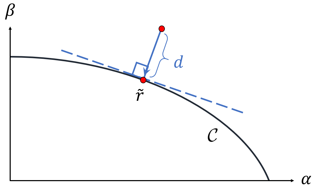
Figure 1: Perpendicular distance $d$ of a nearby point (around $\tilde{r}$) from the critical curve $\mathcal{C}$ [Eq. (3.3)] on a distant observer’s screen [Eq. (3.1)].

By expanding the angular integrals $G_{i}$ in $\varepsilon$, we have $G_{i}\approx\tilde{G}_{i}(\tilde{\lambda},\tilde{q})$. On the other hand, we may compute the leading order radial integrals approximately (see Appendix A). It is convenient to introduce a dimensionless quantity $\delta r_{0}$ to describe the near-criticality [see Eq. (A.8)],

$$\delta r_{0}^{2}=\frac{\tilde{\Delta}}{2\tilde{r}^{2}\tilde{\chi}}\left[\frac{\tilde{q}^{2}}{\tilde{r}^{2}}\delta q-\frac{\tilde{\lambda}}{a}\left(\frac{\tilde{r}-3M}{\tilde{r}-M}\right)\delta\lambda\right].$$

This quantity can be connected with the perpendicular distance $d$ from the critical curve for each choice of a $\tilde{r}$ through (see Fig. 1 and Sec. 3 for details) [10]

$$d=\frac{\delta r_{0}^{2}}{\sqrt{(\partial_{\alpha}\delta r_{0}^{2})^{2}+(\partial_{\beta}\delta r_{0}^{2})^{2}}}=\delta r_{0}^{2}\left[\frac{\tilde{\Delta}}{2\tilde{r}^{4}\tilde{\chi}}\sqrt{\tilde{\beta}^{2}+\left[\tilde{\alpha}-\left(\frac{\tilde{r}+M}{\tilde{r}-M}\right)a\sin{\theta_{o}}\right]^{2}}\right]^{-1}.$$ (2.38)

If $\delta r_{0}=0$, then it is for the precisely critical rays and the radial integrals are given in Eqs. (2.29) and (2.30). If $\delta r_{0}\neq 0$, the radial integrals becomes (see Appendix A) [10]

$$I_{r}\approx-\frac{1}{2\tilde{r}\sqrt{\tilde{\chi}}}\log[C_{\pm}(r_{s},\tilde{r})d],$$ (2.39)

$$I_{\phi}\approx a\left(\frac{\tilde{r}+M}{\tilde{r}-M}+\frac{Q}{\tilde{\Delta}}\right)I_{r}+D_{\pm}(r_{s},\tilde{r}),$$ (2.40)

$$I_{t}\approx\tilde{r}^{2}\left(\frac{\tilde{r}+3M}{\tilde{r}-M}\right)I_{r}+H_{\pm}(r_{s},\tilde{r}),$$ (2.41)

where $C_{\pm}(r_{s},\tilde{r})$, $D_{\pm}(r_{s},\tilde{r})$ and $H_{\pm}(r_{s},\tilde{r})$ are independent of $d$ and can be obtained from the results in Appendix A. We also give an example for the expressions of $C_{\pm}$, $D_{\pm}$ and $H_{\pm}$ in Appendix A.3.

By using the relations (2.25) and (2.26), together with (2.39), (2.40) and (2.41), and expressing $\tilde{G}_{i}$ in terms of elliptical integrals, the lens equations (2.19), (2.20) and (2.21) can be expanded as

$$d\approx\frac{1}{C_{\pm}}e^{-2n\gamma},\qquad\Delta\phi\approx 2n[\delta-2\pi H(\tilde{r}-\tilde{r}_{0})]-J^{\phi}_{\pm},\qquad\Delta t\approx 2n\tau-J^{t}_{\pm}$$ (2.42)

where

$$J^{\phi}_{\pm}=\pm_{o}\frac{\tilde{\lambda}\tilde{\Pi}}{a\sqrt{-\tilde{u}_{-}}}\left[(-1)^{m}[\frac{\tilde{F}_{s}}{\tilde{K}}-\frac{\tilde{\Pi}_{s}}{\tilde{\Pi}}]-[\frac{\tilde{F}_{o}}{\tilde{K}}-\frac{\tilde{\Pi}_{o}}{\tilde{\Pi}}]\right]-D_{\pm}(r_{s},\tilde{r}),$$ (2.43)

$$J^{t}_{\pm}=\mp_{o}\frac{2a\tilde{u}_{+}}{\sqrt{-\tilde{u}_{-}}}\tilde{E}^{\prime}\left[(-1)^{m}[\frac{\tilde{F}_{s}}{\tilde{K}}-\frac{\tilde{E}^{\prime}_{s}}{\tilde{E}^{\prime}}]-[\frac{\tilde{F}_{o}}{\tilde{K}}-\frac{\tilde{E}^{\prime}_{o}}{\tilde{E}^{\prime}}]\right]-H_{\pm}(r_{s},\tilde{r}).$$ (2.44)

These near-critical lens equations (2.42) determine the higher-order images which will be discussed in detail in Sec. 5.

3 Observer’s screen and critical curve

We now introduce screen coordinates to describe the image positions of light sources relative to a distant static observer. The screen coordinates can be defined by using the reception angles of photons reaching the observer. Regarding to the observed inclination $\theta_{o}$ relative to the spin axis of the black hole, we will consider the off-axis and on-axis cases separately.

First we consider an off-axis observer at $r_{o}\rightarrow\infty$ and $0<\theta_{o}<\pi/2$. For such an observer, we can set $\phi_{o}=0$ due to the axisymmetry of the spacetime. It is convenient to use the well-established Cartesian coordinates $(\alpha,\beta)$ to cover its screen, which are expressed in terms of the impact parameters $(\lambda,\eta)$ as [42]

$$\alpha=-\frac{\lambda}{\sin{\theta_{o}}}\ ,\qquad\beta=\pm_{o}\sqrt{\eta+a^{2}\cos^{2}{\theta_{o}}-\lambda^{2}\cot^{2}{\theta_{o}}}\ .$$ (3.1)

Note that we have $\pm_{o}=\text{sign}(\beta)$ in this case. We may also transfer $(\alpha,\beta)$ to a pair of polar coordinates $(\rho,\varphi)$ through

$$\rho=\sqrt{\alpha^{2}+\beta^{2}}=\sqrt{\eta+a^{2}\cos^{2}\theta_{o}+\lambda^{2}},\qquad\tan\varphi=\frac{\beta}{\alpha}.$$ (3.2)

Photons arrivaling with critical impact parameters $[\tilde{\lambda}(\tilde{r}),\tilde{\eta}(\tilde{r})]$ [see Eqs. (2.27) and (2.28)] provide a critical curve on the screen

$$\mathcal{C}=\left\{[\tilde{\alpha}(\tilde{r}),\tilde{\beta}(\tilde{r})]\,\Big{|}\,\tilde{r}_{-}<\tilde{r}<\tilde{r}_{+}\right\},$$ (3.3)

which is parameterized by $\tilde{r}$. Therefore, a point on the critical curve $\mathcal{C}$ can also be depicted with $[\tilde{r},\text{sign}(\tilde{\beta})]$. We show several examples for the critical curve observed off the pole on the middle and right columns of Fig. 2. In the following discussions, we select two inclination angles for the off-pole observers. One is at $\theta_{o}=17^{\circ}$, the same as in the M87* observations in EHT, and the other is at $\theta_{o}=80^{\circ}$, nearly edge-on scenario which is quite different from the M87* case.

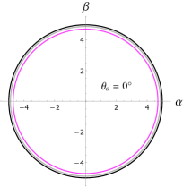
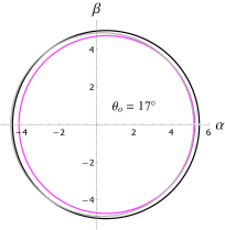
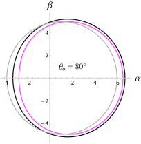
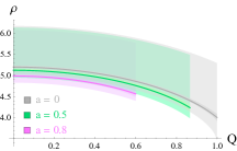
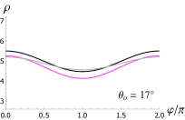
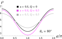
Figure 2: Critical curves $\mathcal{C}$ for the selected black hole parameters. Left column: above we show $\mathcal{C}$ in the Cartesian coordinates (3.5), and below we show the dependence of $\tilde{\rho}$ (central lines in the colored bands), $\Delta\rho^{(1)}$ (lighter colored bands) and $\Delta\rho^{(2)}$ (darker colored bands) on black hole spin $a$ and charge $Q$ in the polar coordinates (3.4). Here $\Delta\rho^{(m)}$ [Eq. (5.6)] represents the width of the $m$-th image ring for an equatorial source ring with $r_{s}\in(r_{+},\infty)$. Middle and right columns: we show $\mathcal{C}$ in the Cartesian coordinates (3.1) (above) and polar coordinates (3.2) (below).

Next we consider an on-axis observer at $r_{o}\rightarrow\infty$ and $\theta_{o}=0$. The photons reaching such an observer would always have zero azimuthal angular momentum and negative polar momentum, that is $\lambda=0$ and $\pm_{o}=\text{sign}(p^{\theta}_{o})=-1$. Then there is only $\eta$ left for a free parameter to use, and both of the choices (3.1) and (3.2) are no longer good in this case. Nevertheless, since the spacetime is axisymmetric relative to the on-axis observer, the angle of arrival photons $\phi_{o}$ can also serve as an independent parameter to describe the image. Therefore, we may introduce another pair of polar coordinates $(\rho,\varphi)$ to cover its screen, which varied from (3.2) to [10]

$$\rho=\sqrt{\eta+a^{2}},\qquad\varphi=\phi_{o}.$$ (3.4)

We may also define the Cartesian coordinates

$$\alpha=\rho\cos\varphi,\qquad\beta=\rho\sin\varphi,$$ (3.5)

for an on-axis observer. When observed form the pole, the critical curve $\mathcal{C}$ is a circle at radius $\tilde{\rho}=\sqrt{\tilde{\eta}+a^{2}}$ and this curve is instead parameterized by the angle $\varphi$. In this case, the perpendicular distance from the critical curve to a point $(\rho,\varphi)$ is then given by $d=\rho-\tilde{\rho}$. We show several examples for the critical curve observed on the pole on the left column of Fig. 2.

4 Observational appearance

In this section, we consider the optical appearances of a spherical source and a thin equatorial disk. We assume axissymmetric for the sources, then the shape of each source can be described by a given function of $r_{s}$ and $\theta_{s}$. Note that we should consider both the direct ($\omega=0)$ and reflected ($\omega=1)$ emissions for radial integrals (2.16) and consider $m\geq 0$ for angular integrals (2.17). Thus we have a series of imaging maps between each source and an observer’s screen, which gives multi-level images: the first (primary), second (secondary) and third images are respectively for $m=0$, $1$, $2$ when viewed form the pole (or respectively for $\bar{m}=0$, $1$, $2$ in Eq. (4.8) when viewed from inclined observers), and the higher-order images are for $m\geq 2$ or $\bar{m}\geq 2$. Here we focus on the primary images and a few lower-order images and discuss the overall feature of these images by applying the lens equations (2.19), (2.20) and (2.21), while the higher-order images will be discussed in detail in the next section by using the near-critical lens equations (2.42).

4.1 Spherical source viewed by an on-axis observer

We now discuss the image positions of a spherical source viewed by an on-axis observer from above ($\theta_{o}=0$ and $\pm_{o}=-1$). For a spherical source we have

$$r_{s}=\text{const},\qquad\theta_{s}\in(0,\pi),$$ (4.1)

then Eq. (2.19) becomes

$$I^{(\omega)}_{r}(r_{s},\rho)=\frac{1}{\sqrt{\rho^{2}-a^{2}}}[(2m+1)K(\rho)\pm_{s}F(\theta_{s},\rho)].$$ (4.2)

Inserting this for a sphere with radius $r_{s}$, we get the transfer function $\cos\theta_{s}(\rho)|_{r_{s}}$[41],

$$\cos{\theta_{s}}=\text{cd}\left(\sqrt{\rho^{2}-a^{2}}I(\rho)\bigg{|}\frac{a^{2}}{a^{2}-\rho^{2}}\right),$$ (4.3)

where “cd” is the Jacobi cd function. Notice that, due to the periodicity of the elliptic function $K$, the first term on the right side of Eq. (4.2) does not contribute. This transfer function shows directly the connection between the emission latitude $\theta_{s}$ on the emission sphere and the observed radius $\rho$ on the observer’s screen. In Fig. 3, we show several transfer functions $\cos\theta_{s}(\rho)|_{r_{s}}$ for selected values of black hole parameters $a$ and $Q$. Meanwhile, we consider distinct cases for source radii such that $r_{s}<\tilde{r}_{0}$, $\tilde{r}_{0}<r_{s}\ll r_{o}$, $r_{s}\sim r_{o}$ and $\tilde{r}_{0}\ll r_{s}\ll r_{o}$, respectively. For $\rho<\tilde{\rho}$, the transfer function (4.3) is single-valued, corresponding to only the direct emission. For $\rho>\tilde{\rho}$, the transfer function (4.3) becomes double-valued, corresponding to both the direct and reflected emissions. Each oscillation of $\theta_{s}$ from $0$ to $\pi$ corresponds to an image of the source sphere. Near the critical radius $\rho=\tilde{\rho}$, the oscillations become extremely dense, which corresponds to infinitely many images labeled with $m$. We can see that, the primary image in each case mainly reflects the property of the source, while the higher-order images reflect the property of the spacetime which are almost independent of the source directly. A remarkable feature of the the higher-order images is that these images in each plot approach the critical curve at $\rho=\tilde{\rho}$ in a narrow region. As the charge $Q$ or spin $a$ varies, the position of $\tilde{\rho}$ is changed correspondingly (see Fig. 2).

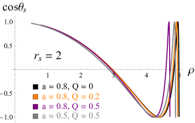
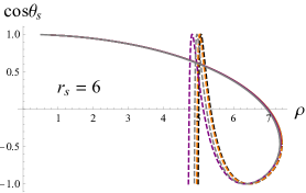
\begin{overpic}[scale={0.4}]{cs100.pdf} \put(15.0,22.0){\includegraphics[scale={0.3}]{cs100fine.pdf}} \end{overpic}

\begin{overpic}[scale={0.4}]{cs1000.pdf} \put(15.0,22.0){\includegraphics[scale={0.3}]{cs1000fine.pdf}} \end{overpic}

Figure 3: Transfer functions $\cos\theta_{s}(\rho)$ for spherical sources with radii $r_{s}=2,\,6,\,100$ and $1000$ viewed from an on-axis observer at $r_{o}=100$. Solid and dashed lines have $\omega=0$ and $1$, respectively.

4.2 Thin equatorial disk viewed by an on-axis observer

We now discuss the images of an equatorial thin disk consisting of emitting rings with $r_{s}>r_{+}$ and $\theta_{s}=\pi/2$, viewed by an on-axis observer from above ($\theta_{o}=0$ and $\pm_{o}=-1$). We first consider the apparent positions of the source rings. From Eq. (2.19) we have

$$I_{r}^{(\omega)}(r_{s},\rho)=\frac{1}{\sqrt{\rho^{2}-a^{2}}}(2m+1)K\left(\frac{a^{2}}{a^{2}-\rho^{2}}\right).$$ (4.4)

This gives a series of transfer functions ${r_{s}}^{(m)}(\rho)$ for $m=0,1,2,\dots$, respectively. Different from the spherical case [Eq. (4.2)], for each certain $m$, Eq. (4.4) is solved either by the direct ray with $\omega=0$ or by the reflected ray with $\omega=1$, and in no case can both of rays solve this equation. We will consider a disk model that extends to the event horizon $r_{+}$. In Fig.[4], we show the first three transfer functions, $r_{s}^{(0)}(\rho)$, $r_{s}^{(1)}(\rho)$ and $r_{s}^{(2)}(\rho)$, under different black hole parameters. We can see that the properties of the disk images at different orders are similar as those of the spherical case. For a black hole with certain parameters, the first transfer function $r_{s}^{(0)}(\rho)$ is approximately linear, $r_{s}\approx\rho-1$, representing that the primary image is a direct reflection of the source. Note that the lower bound of $\rho$ on the screen corresponds to $r_{s}=r_{+}$. The slope of the transfer function $dr_{s}/d\rho$ becomes larger as the image level goes higher, which corresponds to narrower and narrower bands covering the critical radius $\tilde{\rho}$ on the screen. Like in the spherical case, the black hole charge $Q$ and spin $a$ also affect the position of $\tilde{\rho}$. Besides, we see from Fig. 2 that the charge and spin affect the widths of the first and second narrow bands ($\Delta\rho^{(1)}$ and $\Delta\rho^{(2)}$) as well. Thus, the higher-order images again show the dependence on the spacetime parameters clearly.

Next, we consider the change of azimuthal angles between the angles at arrival $\phi_{o}$ and at emission $\phi_{s}$. From Eq. (2.20) we have

$$\Delta\phi^{(m)}=\phi^{(m)}_{o}-\phi_{s}=I_{\phi}(r_{s},\rho^{(m)}(r_{s}))+m\pi,$$ (4.5)

where we have used Eq. (2.33) for the pole-crossing orbits to get the last term. For convenience, we introduce $[\Delta\phi]=\mod_{2\pi}(\Delta\phi)$. In Fig. 4, we show the results of $[\Delta\phi^{(0)}]$, $[\Delta\phi^{(1)}]$ and $[\Delta\phi^{(2)}]$ as functions of $\rho$. Note that a static disk cannot exist inside the ergosphere at $r_{e}$, therefore we only show the results for $r_{s}\in(r_{e},\infty)$. We can see that for a black hole with given parameters $a$ and $Q$, the images with even $m$ have $[\Delta\phi]\in(0,\pi)$ while those with odd $m$ have $[\Delta\phi]\in(\pi,2\pi)$. For the primary image, the influence of black hole parameters on $[\Delta\phi]$ is quite small in general, while the influences become larger and larger as the image level goes higher. For the images at each level, $[\Delta\phi]$ increases with the spin $a$ or the charge $Q$, and the influence of spin is overall greater than that of charge.

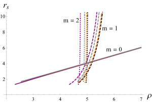
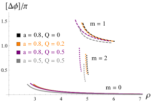
Figure 4: Left: positions of the images of an equatorial disk with $r_{s}\in(r_{+},\infty)$ viewed by an on-axis observer at $r_{o}=1000$. Right: changes of azimuthal angles of the images of an equatorial disk with $r_{s}\in(r_{e},\infty)$ viewed by an on-axis observer at $r_{o}=1000$.

4.3 Thin equatorial disk viewed by an off-axis observer

We now discuss the images of an equatorial thin disk consisting of emitting rings with $r_{s}>r_{+}$ and $\theta_{s}=\pi/2$, viewed by an off-axis observer [$\theta_{o}\neq 0$ and $\pm_{o}=\text{sign}(\beta)$]. We first consider the apparent positions of the equatorial emitting rings. The position of $m$-th image (denoted as ${\mathcal{C}}_{m}$) of a equatorial ring at $r_{s}$ is determined by Eq.(2.19) which now becomes

$${\mathcal{C}}_{m}:\ I_{r}^{(\omega)}(r_{s},\alpha,\beta)=\frac{1}{a\sqrt{-u_{-}(\alpha,\beta)}}[2mK(\alpha,\beta)-\text{sign}(\beta)F_{o}(\alpha,\beta)].$$ (4.6)

However, due to the appearance of $\text{sign}(\beta)$ in the last term, $m$ is no longer a good quantities to label continuous images for an inclined observer. When crossing the $\alpha$-axis, Eq. (4.6) yields

$${\mathcal{C}}_{m}:\ I_{r}^{(\omega)}(r_{s},\alpha)=\begin{cases}\frac{1}{a\sqrt{-u_{-}(\alpha)}}(2m-1)K(\alpha)&\text{if}\,\,\,\beta\rightarrow 0^{+},\\ \frac{1}{a\sqrt{-u_{-}(\alpha)}}(2m+1)K(\alpha)&\text{if}\,\,\,\beta\rightarrow 0^{-}.\end{cases}$$ (4.7)

Note that ${\mathcal{C}}_{m}(\beta\rightarrow 0^{-})={\mathcal{C}}_{m+1}(\beta\rightarrow 0^{+})$, which means that the lower part image of ${\mathcal{C}}_{m}$ and the upper part image of ${\mathcal{C}}_{m+1}$ can be smoothly connected. Thus we can instead introduce

$$\bar{m}=m-H(\beta)$$ (4.8)

as a label for continuous images, where $H$ is the Heaviside function. That is, we have $\{{\mathcal{C}}_{\bar{m}},\bar{m}=0,1,2\dots\}=\{{\mathcal{C}}_{m}(\beta<0)\cup{\mathcal{C}}_{m+1}(\beta>0),\,m=0,1,2,\dots\}$, this gives a set of smooth curves on the observer’s screen. Moreover, one finds that $\bar{m}$ denotes how many times that a photon passes across the equatorial plane before it reaching the screen. We will consider three source rings lying in the ranges $3<r_{s}<3.5$, $6<r_{s}<6.5$ and $9<r_{s}<9.5$, and consider three choices for the black hole parameters $a$ and $Q$. In Fig.[5], we show the first two ($\bar{m}=0,\,1$) images of each selected equatorial source ring for each choice of the black hole parameters. We also describe the first two image rings of source rings at $r_{s}=3$ and $7$ with the polar coordinates $(\rho,\varphi)$ [Eq. (3.2)] in Fig.[6], to quantitatively show the variation of radius $\rho$ along polar angle $\varphi$ for each image. We can see that, again, the primary images mainly reflect the feature of source profile (the inner bound $r_{+}$ of the disk) while the higher-order images become less dependent on the source detail and mainly reflect the property of the spacetime (the critical curve $\mathcal{C}$).

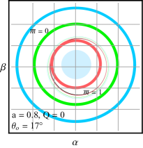
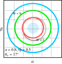
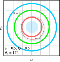
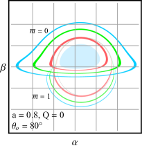
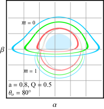
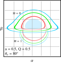
Figure 5: Images positions of equatorial rings with $r_{s}\in[3,3.5]$ (pink), $r_{s}\in[6,6.5]$ (green) and $r_{s}\in[9,9.5]$ (blue) described in Cartesian coordinates (3.1). In each plot, the darker and lighter rings correspond to $\bar{m}=0,1$, respectively, the center lightblue region is the inner shadow [43] with the edge corresponds to a direct map of $r_{+}$, and the black ring corresponds to the critical curve.

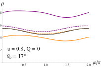
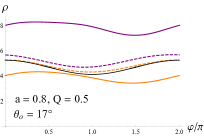
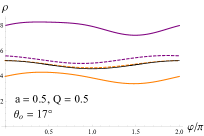
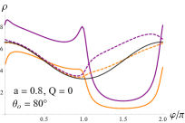
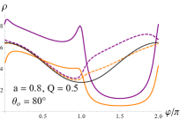
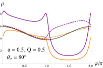
Figure 6: Images positions of equatorial rings at $r_{s}=3$ (orange) and $r_{s}=7$ (purple) described in polar coordinates (3.2). In each plot, the solid and dashed curves correspond to $\bar{m}=0,1$, respectively, and the black curve corresponds to the critical curve.

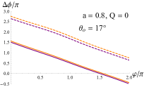
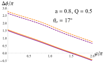
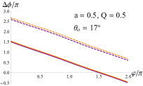
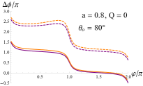
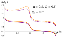
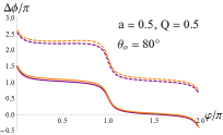
Figure 7: Image rotations $\Delta\phi$ of equatorial rings at $r_{s}=3$ (orange) and $r_{s}=7$ (purple) described in polar coordinates (3.2). In each plot, the solid and dashed curves correspond to $\bar{m}=0,1$, respectively.

Next, we consider the change of azimuthal angles between the angles at arrival $\phi_{o}$ and at emission $\phi_{s}$. Rewriting Eq. (2.20) in terms of the polar coordinates (3.2) we get

$$\Delta\phi=\rho\cos{\varphi}\sin{\theta_{o}}G_{\phi}^{(\bar{m})}(\rho,\varphi)-I^{(\omega)}_{\phi}(r_{s},\rho,\varphi).$$ (4.9)

Note that for an off-axis observer we can set $\phi_{o}=0$, then we have $\Delta\phi=-\phi_{s}$. Therefore, this equation actually gives the relation between the source position $\phi_{s}$ and its image position on the observer’s screen. We show this relation for selected black hole parameters and observer’s inclinations in Fig.[7]. We find that in each plot the primary image is very close to the optical images of inclined source rings in flat spacetime, while the secondary image is rotated by roughly $\sim\pi$ relative to primary image, showing the lensing effects of black hole. We can also see that the image’s rotation depends on the position $\varphi$ along the image ring, the black hole spin $a$ and the charge $Q$. We will study the rotations in more detail in next section.

5 Photon ring (higher-order images)

In the previous section, we have discussed the overall appearances of various sources. In this section, we will move on to the details of higher-order images, which altogether form the so-called photon ring on the screen. The photon ring is composed of the photons arriving near the critical curve $\mathcal{C}$. We have introduced the near-critical lens equations (2.42) in Sec. 2.2, which determine the behaviors of successive higher-order images. Here we will discuss the property of photon ring for various sources in terms of the key parameters $\gamma$, $\delta$ and $\tau$, viewed on or off the pole. In particular, we will study the dependence of these parameters on the black hole spin $a$ and charge $Q$.

5.1 Sources viewed by an on-axis observer

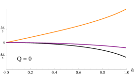
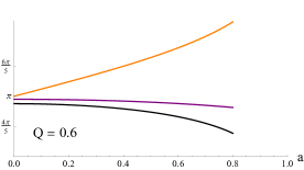
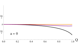
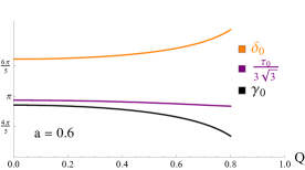
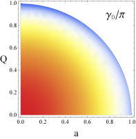
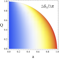
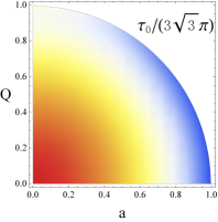
Figure 8: The key parameters $\gamma_{0}$, $\delta_{0}$ and $\tau_{0}$ for an on-axis observer. Top: we show the influences of spin $a$ on these parameters for black holes with charge $Q=0$ (left) and $Q=0.6$ (right). Middle: we show the influences of charge $Q$ on these parameters for black holes with spin $a=0$ (left) and $a=0.6$ (right). Bottom: we show the density plots of these parameters on the $(a,\,Q)$ plane within the whole allowed range for $a$ and $Q$.

We first consider a general source viewed by an on-axis observer using the near-critical equations (2.42). In this case, we have $\theta_{o}=0$, thus $\pm_{o}=-1$, $F_{o}=K$, $\Pi_{o}=\Pi$ and $E^{\prime}_{o}=E^{\prime}$. Moreover, the photon shell radii $\tilde{r}\in(\tilde{r}_{-},\tilde{r}_{+})$ reduces to a single photon sphere radius $\tilde{r}_{0}$, and the key parameters $\gamma$ [Eq. (2.32)], $\delta$ [Eq. (2.35)] and $\tau$ [Eq. (2.36)] reduce to $\gamma_{0}$, $\delta_{0}$ and $\tau_{0}$, respectively. The critical parameters $\gamma_{0}$, $\delta_{0}$ and $\tau_{0}$ are independent of the position around a critical curve. Now we consider successive images labeled with $m$ and $m+1$, then from Eqs. (2.42) we can obtain [10]

$$\frac{d_{m+1}}{d_{m}}\approx\exp\left[-[1+(-1)^{m}\frac{\tilde{F}_{s}}{\tilde{K}}]\gamma_{0}\right],$$ (5.1)

$$(\Delta\phi)_{m+1}-(\Delta\phi)_{m}\approx[1+(-1)^{m}\frac{\tilde{F}_{s}}{\tilde{K}}]\delta_{0}-(-1)^{m}\frac{\tilde{F}_{s}}{\tilde{K}}\pi,$$ (5.2)

$$(\Delta t)_{m+1}-(\Delta t)_{m}\approx[1+(-1)^{m}\frac{\tilde{F}_{s}}{\tilde{K}}]\tau_{0}+(-1)^{m}\frac{4a\tilde{u}_{+}}{\sqrt{-\tilde{u}_{-}}}\tilde{E}^{\prime}[\frac{\tilde{F}_{s}}{\tilde{K}}-\frac{\tilde{E}^{\prime}_{s}}{\tilde{E}^{\prime}}].$$ (5.3)

We have used Eq. (2.33) for the pole-crossing orbits to obtain the last term in Eq. (5.2). Note that $d=\rho-\tilde{\rho}$ for the on-axis case and $C_{\pm},D_{\pm},H_{\pm}$ in Eqs. (2.42) were dropped out from the final results. If we consider the images that execute $m$ and $m+2$ angular turnings, the above equations are simplified dramatically, and reduce to

$$\frac{d_{m+2}}{d_{m}}\approx e^{-2\gamma_{0}},\qquad(\Delta\phi)_{m+2}-(\Delta\phi)_{m}\approx 2\delta_{0},\qquad(\Delta t)_{m+2}-(\Delta t)_{m}\approx 2\tau_{0}.$$ (5.4)

Next, we consider an equatorial source, for which we have $\theta_{s}=\pi/2$, $F_{s}=0$, $\Pi_{s}=0$ and $E^{\prime}_{s}=0$. Then from Eqs. (5.1), (5.2) and (5.3) we get

$$\frac{d_{\text{eq},m+1}}{d_{\text{eq},m}}\approx e^{-\gamma_{0}},\qquad(\Delta\phi)_{\text{eq},m+1}-(\Delta\phi)_{\text{eq},m}\approx\delta_{0},\qquad(\Delta t)_{\text{eq},m+1}-(\Delta t)_{\text{eq},m}\approx\tau_{0}.$$ (5.5)

Now we consider the $m$-th image ring for an equatorial source ring with $r_{s}\in(r_{s-},\,r_{s+})$. We use $\rho^{(m)}_{\pm}$ to denote the outer/inner edges for the image ring. Recalling that $d_{\pm}=\rho_{\pm}-\tilde{\rho}$, then the position $\rho^{(m)}_{\pm}$ can be obtained from Eq. (2.42) and the width of the $m$-th image ring is given by

$$\Delta\rho^{(m)}=\rho^{(m)}_{+}-\rho_{-}^{(m)}.$$ (5.6)

It follows from Eq. (2.42) that $\Delta\rho^{(m+1)}/\Delta\rho^{(m)}\approx e^{-\gamma_{0}}$, meaning that successive images are narrower by a factor of $e^{-\gamma_{0}}$.

The above expressions [from Eq. (5.1) to Eq. (5.5)] have the same form as those for the Kerr case [10], however, the effects of charge $Q$ were included implicitly. Like in the Kerr case, we can see that the three key parameters still control the behaviors of successive images in the KN case. The parameters $\gamma_{0}$, $\delta_{0}$ and $\tau_{0}$ encode the effects of demagnification, angle lapse and time delay, respectively, between successive images. For a general source, even though these effects are not precisely encoded by $\gamma_{0}$, $\delta_{0}$ and $\tau_{0}$ when $m$ is shifted to $m+1$ [see Eqs. (5.1), (5.2) and (5.3)], the effects become evident when we consider images with $m$ and $m+2$. As we can see from Eq. (5.4) that, relative to the images at $m$ level, those at $m+2$ level have demagnification $2\gamma_{0}$, rotation $2\delta_{0}$ and time delay $2\tau_{0}$. For an equatorial source, we can further see from Eq. (5.5) that each successive image has demagnification $\gamma_{0}$, rotation $\delta_{0}$ and time delay $\tau_{0}$ relative to the reference image. In order to see the influences of spin $a$ and charge $Q$, we show the three key parameters for black holes with different choices of $a$ and $Q$ in Fig. 8.

5.2 Sources viewed by an off-axis observer

We now consider a general source viewed by an off-axis observer, for which we have $\theta_{o}\neq 0$ and $\pm_{o}=\text{sign}(\beta)$. For an off-axis observer, the key parameters $\gamma$, $\delta$ and $\tau$ depend on $\tilde{r}$ nontrivially [see Eqs. (2.32), (2.35) and (2.36)]. Near a fixed point $[\tilde{r},\text{sign}(\tilde{\beta})]$ on the critical curve, the near-critical lens equations (2.42) for successive images become [10]

$$\frac{d_{m+1}}{d_{m}}\approx\exp\left[-[1-\text{sign}(\beta)(-1)^{m}\frac{\tilde{F}_{s}}{\tilde{K}}]\gamma\right],$$ (5.7)

$$(\Delta\phi)_{m+1}-(\Delta\phi)_{m}\approx[1-\text{sign}(\beta)(-1)^{m}\frac{\tilde{F}_{s}}{\tilde{K}}]\hat{\delta}+\text{sign}(\beta)(-1)^{m}\frac{2\tilde{\lambda}\tilde{\Pi}}{a\sqrt{-\tilde{u}_{-}}}[\frac{\tilde{F}_{s}}{\tilde{K}}-\frac{\tilde{\Pi}_{s}}{\tilde{\Pi}}],$$ (5.8)

$$(\Delta t)_{m+1}-(\Delta t)_{m}\approx[1-\text{sign}(\beta)(-1)^{m}\frac{\tilde{F}_{s}}{\tilde{K}}]\tau-\text{sign}(\beta)(-1)^{m}\frac{4a\tilde{u}_{+}}{\sqrt{-\tilde{u}_{-}}}\tilde{E}^{\prime}[\frac{\tilde{F}_{s}}{\tilde{K}}-\frac{\tilde{E}^{\prime}_{s}}{\tilde{E}^{\prime}}],$$ (5.9)

where $\hat{\delta}=\delta-2\pi H(\tilde{r}-\tilde{r}_{0})$, and the functions $C_{\pm}$, $D_{\pm}$ and $H_{\pm}$ in Eqs. (2.42) were dropped out again from the final results.

For the images labeled with $m$ and $m+2$, we can still get similar expressions as Eqs. (5.4), in which the key parameters $\gamma_{0},\,\delta_{0},\,\tau_{0}$ are replaced by those without the subscript. Likewise, for an equatorial source, Eqs. (5.5) still hold for the off-axis case once we made the same minor replacement for the key parameters.

When a given source is observed off the pole, the key parameters $\gamma$, $\delta$ and $\tau$ also control the behaviors of its successive images. However, in contrast with the on-axis case, the parameters for the off-axis case depend on the position $\tilde{r}$ along the critical curve $\mathcal{C}$. Near each point on the critical curve, the properties of successive images are the similar as those for the on-axis case described above in Sec. 5.1 and we will not repeat them again. In Fig. 9 we show the value of the key parameters along the critical curve for selected inclination $\theta_{o}$, spin $a$ and charge $Q$.

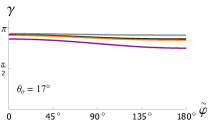
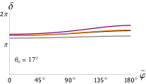
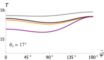
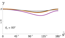
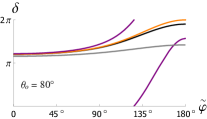
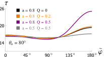
Figure 9: The key parameters $\gamma$, $\delta$ and $\tau$ for off-axis observers with inclinations $\theta_{o}=17^{\circ}$ (above) and $80^{\circ}$ (below). For several selected choices of black hole parameters $a$ and $Q$, we show the values of the key parameters along the critical curve which is parameterized by the polar coordinate $\tilde{\varphi}$ [see Eq. (3.2)].

6 Summary and discussion

In this paper, we studied the lensing effects of charged rotating KN black holes, closely following the work [10] on the lensing by Kerr black holes. Comparing with the results in Kerr case, we found the modifications in the integral form of the photon motion and three key parameters $\gamma$, $\delta$ and $\tau$ of critical photon emissions induced by the charge $Q$ of a KN black hole, see (2.29), (2.30), (2.32), (2.35) and (2.36). Then we investigated the optical appearances of luminous sources around KN black holes, and our main results can be seen in Fig. 2 to Fig. 9. In particular, we paid special attention to the higher-order images ($\bar{m}\geq 2$) of luminous sources, which have not been discussed carefully in the literature.

From our studies, we noticed that for the primary and secondary images the effect of $Q$ are not evident, see Fig. 4 to Figs. 7. However it is worth emphasizing that the charge $Q$ would have a significant effect for higher-order images, see Figs. 8 and 9. The reason why the charge $Q$ is able to have a noticeable effect on the higher-order images is that the photon emissions of higher order images are closer to the critical curve $\mathcal{C}$. Since the lights travel around the black hole more times before reaching the observer, the higher-order images can encode more information of critical curve. On the other hand, from Fig. 2, we can see that the charge $Q$ has a nonnegligible effect on the critical curve. As a result, it is quite reasonable that charge $Q$ would give a detectable effect on higher-order images. We believe that as the observational accuracy of EHT improves [44, 45, 46], observations of higher-order images will become feasible and allows us to constrain the black hole parameters, including the charge [12, 24, 27, 29, 33, 47].

Appendix A Radial integrals for near-critical rays

In this appendix, we will compute the radial integrals for near-critical rays following [10]. We will outline the main steps and provide the final results for reference.

A.1 Asymptotic expansions

For the light rays crossing the equatorial plane we may introduce a nonnegative parameter $q=\sqrt{\eta}$ for convenience. For near-critical rays, the impact parameters can be written as

$$\lambda=\tilde{\lambda}(1+\delta\lambda),\qquad q=\tilde{q}(1+\delta q),$$ (A.1)

with $|{\delta\lambda}|\sim|{\delta q}|\sim\varepsilon\ll 1$. We introduce the $\delta r$-coordinate around the critical radius $\tilde{r}$ as well

$$r=\tilde{r}(1+\delta r).$$ (A.2)

Then we can define the near and far regions as follows,

$$\text{Near region}:\qquad|\delta r|\ll 1,$$ (A.3)

$$\text{Far region}:\quad\quad\,\,\,\,|\delta r|\gg\varepsilon.$$ (A.4)

The far region is disjoint around $\tilde{r}$, as can be seen in Fig.10. Apparently, there are overlapping regions here in which $\varepsilon\ll|\delta r|\ll 1$. This ensures the usability of the matched asymptotic expansion (MAE) method.

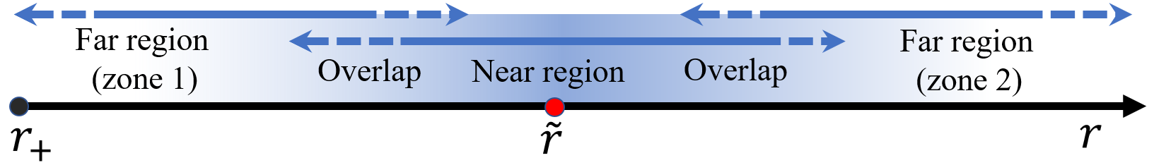
Figure 10: Schematic diagram for near, far and overlapping regions with regards to $\tilde{r}$. Note that zone 1 ($\delta r<0$) and zone 2 ($\delta r>0$) are in two disjoint far regions.

In the near region, the radial potential $\mathcal{R}(r)$ may be expanded in the regime $|\delta r|\sim\sqrt{\varepsilon}$, then

$$\mathcal{R}(r)=\frac{1}{2}\mathcal{R}^{\prime\prime}(\tilde{r})\delta r^{2}+\mathcal{R}_{\lambda}\delta\lambda+\mathcal{R}_{q}\delta q+\mathcal{O}(\varepsilon^{3/2}),$$ (A.5)

where

$$\mathcal{R}^{\prime\prime}(\tilde{r})=\tilde{r}^{2}(6\tilde{r}^{2}+a^{2}-\tilde{\lambda}^{2}-\tilde{q}^{2}),\quad\mathcal{R}_{\lambda}=-2\tilde{\lambda}\tilde{r}\Delta(\tilde{r})\frac{2Q-3M\tilde{r}+\tilde{r}^{2}}{a(M-\tilde{r})},\quad\mathcal{R}_{q}=-2\tilde{q}^{2}\Delta(\tilde{r}).$$ (A.6)

It is convenient to define

$$\mathcal{R}_{n}(\delta r):=\frac{1}{2}\mathcal{R}^{\prime\prime}(\tilde{r})\delta r^{2}+\mathcal{R}_{\lambda}\delta\lambda+\mathcal{R}_{q}\delta q=4\tilde{r}^{4}\tilde{\chi}(\delta r^{2}-\delta r_{0}^{2}),$$ (A.7)

where

$$\delta r_{0}^{2}=\frac{\tilde{\Delta}}{2\tilde{r}^{2}\tilde{\chi}}\left[\frac{\tilde{q}^{2}}{\tilde{r}^{2}}\delta q-\frac{\tilde{\lambda}}{a}\left(\frac{\tilde{r}-3M}{\tilde{r}-M}\right)\delta\lambda\right],\qquad\tilde{\chi}=1-\frac{M\Delta(\tilde{r})}{\tilde{r}(M-\tilde{r})^{2}}.$$ (A.8)

In the far region, we have $|\delta r|\gg\varepsilon$ and the radial potential becomes

$$\mathcal{R}(r)=\mathcal{R}(\tilde{r}(1+\delta r))|_{\lambda=\tilde{\lambda},q=\tilde{q}}+\mathcal{O}(\varepsilon).$$ (A.9)

It is convenient to define

$$\mathcal{R}_{f}(\delta r):=\mathcal{R}(\tilde{r}(1+\delta r))|_{\lambda=\tilde{\lambda},q=\tilde{q}}=4\tilde{r}^{4}\tilde{\chi}\delta r^{2}\mathcal{Q}(\delta r)$$ (A.10)

where

$$\mathcal{Q}(\delta r)=1+\frac{\delta r}{\tilde{\chi}}+\frac{\delta r^{2}}{4\tilde{\chi}}.$$ (A.11)

Similarly, we can also expand the functions $\mathcal{I}_{\phi}$ and $\mathcal{I}_{t}$ [Eq. (2.15)] in the near and far regions, respectively. Then the radial integrals $I_{i}$ ($i=r,\phi,t$) [Eq. (2.13)] can be computed explicitly in each of these regions. Combining the near-zone and far-zone results for a physical photon trajectory by using the MAE method, one can obtain the final results for the radial integrals connecting a source to an observer.

Note that a physical light ray never encounter a turning point in the far region thus we should always have $\mathcal{R}_{f}(\delta r)>0$. On the other hand, a light ray has a turning point $r_{t}$ (corresponding to the larger root of $\mathcal{R}_{n}(\delta r)=0$) in the near region if $\delta r_{0}^{2}>0$. In that case, $r_{t}=\tilde{r}(1+\delta r_{0})$. We have described in Sec. 2.2 that $\delta r_{0}^{2}$ is related to the perpendicular distance $d$ from the critical curve and $\delta r_{0}^{2}\gtrless 0$ corresponds to the rays arriving outside/inside the critical curve, respectively.

A.2 Matched asymptotic expansion computations

In the near region, we use $I^{n}_{i}(\delta r_{a},\delta r_{b})$ to denote the leading order results in $\varepsilon$ of the radial integral from $\delta r_{a}$ to $\delta r_{b}$ with $\delta r_{a}<\delta r_{b}\ll 1$. The radial integrals in (2.13) can be written as

$$I^{n}_{r}=\frac{1}{2\tilde{r}\sqrt{\tilde{\chi}}}\int_{\delta r_{a}}^{\delta r_{b}}\frac{d(\delta r)}{\sqrt{\delta r^{2}-\delta r_{0}^{2}}},\quad I_{\phi}^{n}=a\left(\frac{\tilde{r}+M}{\tilde{r}-M}+\frac{Q}{\tilde{\Delta}}\right)I_{r}^{n},\quad I_{t}^{n}=\tilde{r}^{2}\left(\frac{\tilde{r}+3M}{\tilde{r}-M}\right)I_{r}^{n}.$$ (A.12)

And the result for $I_{r}^{n}$ is

$$I_{r}^{n}(\delta r_{a},\delta r_{b})=\frac{\text{sign}(\delta r)}{2\tilde{r}\sqrt{\tilde{\chi}}}\log{\left(\frac{|\delta r|+\sqrt{\delta r^{2}-\delta r^{2}_{0}}}{|\delta r_{0}|}\right)}\Bigg{|}^{\delta r_{b}}_{\delta r_{a}}.$$ (A.13)

In one zone of the far region (either in zone 1 or in zone 2 in Fig. 10), we use $I^{f}_{i}(\delta r_{a},\delta r_{b})$ to denote the radial integral from $\delta r_{a}$ to $\delta r_{b}$ with $\varepsilon\ll\delta r_{a}<\delta r_{b}$. The radial integrals in (2.13) can be written as

$$I^{f}_{i}=\frac{1}{2\tilde{r}\sqrt{\tilde{\chi}}}\int_{\delta r_{a}}^{\delta r_{b}}\frac{\mathcal{I}^{f}_{i}(\delta r)d(\delta r)}{\sqrt{\delta r^{2}\mathcal{Q}(\delta r)}},\qquad\mathcal{I}^{f}_{i}(\delta r)=\mathcal{I}_{i}(\tilde{r}(1+\delta r))|_{\lambda=\tilde{\lambda},q=\tilde{q}},$$ (A.14)

where $\mathcal{I}_{i}(r)$ are introduced in (2.15). Following the procedure in [10] we get

$$I_{r}^{f}(\delta r_{a},\delta r_{b})=\frac{1}{2\tilde{r}\sqrt{\tilde{\chi}}}\ \text{sign}(\delta r)\log{\left|\frac{\sqrt{\mathcal{Q}(\delta r)}+\delta r/2\tilde{\chi}+1}{\delta r}\right|}\Bigg{|}^{\delta r_{b}}_{\delta r_{a}},$$ (A.15)

$$I_{\phi}^{f}(\delta r_{a},\delta r_{b})=a\left(\frac{\tilde{r}+M}{\tilde{r}-M}+\frac{Q}{\tilde{\Delta}}\right)I_{r}^{f}(\delta r_{a},\delta r_{b})-\text{sign}(\delta r)\frac{Ma}{\tilde{r}^{2}\sqrt{\tilde{\chi}}}\mathcal{Q}_{\phi}(\delta r)\bigg{|}^{\delta r_{b}}_{\delta r_{a}},$$ (A.16)

$$I_{t}^{f}(\delta r_{a},\delta r_{b})=\tilde{r}^{2}\left(\frac{\tilde{r}+3M}{\tilde{r}-M}\right)I_{r}^{f}(\delta r_{a},\delta r_{b})-\text{sign}(\delta r)\frac{\tilde{r}}{2\sqrt{\tilde{\chi}}}\mathcal{Q}_{t}(\delta r)\bigg{|}^{\delta r_{b}}_{\delta r_{a}},$$ (A.17)

where

$$\mathcal{Q}_{\phi}(\delta r) = -\frac{c_{0}+\delta r}{(\delta r_{+}-\delta r_{-})\delta r_{-}\sqrt{\mathcal{Q}(\delta r)}}\operatorname{arctanh}{\mathcal{Q}_{2}(\delta r,\delta r_{-})}+(\delta r_{-}\leftrightarrow\delta r_{+}),$$ (A.18)

$$\mathcal{Q}_{t}(\delta r) = -4\tilde{\chi}\sqrt{\mathcal{Q}(\delta r)}-\frac{4M\sqrt{\tilde{\chi}}}{\tilde{r}}\operatorname{arctanh}{\mathcal{Q}_{2}(\delta r,\infty)}$$ (A.19)

$$+\left[\frac{c_{1}(1+\delta r_{-})+c_{2}(1+\delta r_{-})^{2}+(1+\delta r_{-})^{4}}{\delta r_{-}(\delta r_{-}-\delta r_{+})\sqrt{\mathcal{Q}(\delta r_{-})}}\operatorname{arctanh}{\mathcal{Q}_{2}(\delta r,\delta r_{-})}+(\delta r_{-}\leftrightarrow\delta r_{+})\right],\qquad\,\,\,\,\,\,$$

with $\delta r_{\pm}$ being the radii of the event horizon in the $\delta r-$coordinates, and

$$c_{0}=1-\frac{a\tilde{\lambda}}{2M\tilde{r}},\quad c_{1}=\frac{2Ma}{\tilde{r}^{3}}(a-\tilde{\lambda}),\quad c_{2}=\frac{a^{2}}{\tilde{r}^{2}},$$ (A.20)

$$\mathcal{Q}_{2}(\delta r_{a},\delta r_{b})=\frac{2\sqrt{\mathcal{Q}(\delta r_{a})\mathcal{Q}(\delta r_{b})}}{\mathcal{Q}(\delta r_{a})+\mathcal{Q}(\delta r_{b})-(\delta r_{a}-\delta r_{b})^{2}/4\tilde{\chi}}.$$ (A.21)

Next we use the MAE method to calculate radial integrals for the photons connecting $|\delta r_{a}|\ll 1$ in the near region to $|\delta r_{b}|\gg\varepsilon$ in the far region through their overlapping region $\varepsilon\ll|\delta R|\ll 1$. There are several distinct scenarios. For the photons arriving outside the critical curve, we have $\delta r_{a}>\delta r_{0}$ such that the point is outside the turning point and we denote the integrals for this case as $I_{i,\text{out}}^{n\rightarrow 2}(\delta r_{a},\delta r_{b})$. For the photons arriving inside the critical curve, we may either have $0<\delta r_{a}<\delta r_{b}$ or $\delta r_{b}<\delta r_{a}<0$ and we denote the corresponding integrals as $I_{i,\text{in}}^{n\rightarrow 2}(\delta r_{a},\delta r_{b})$ and $I_{i,\text{in}}^{1\rightarrow n}(\delta r_{b},\delta r_{a})$, respectively. We have used the superscripts “$1\rightarrow n$” to denote the path integrals from zone 1 of the far region to the near region, and “$n\rightarrow 2$” to denote the path integrals from the near region to zone 2 of the far region (see Fig. 10). We have also used the subscript ”in/out” to denote the photons arriving inside or outside the critical curve, respectively.

We will take $I_{r,\text{out}}^{n\rightarrow 2}(\delta r_{a},\delta r_{b})$ as an example to perform the calculation, and list the results for $I_{\phi,\text{out}}^{n\rightarrow 2}(\delta r_{a},\delta r_{b})$ and $I_{t,\text{out}}^{n\rightarrow 2}(\delta r_{a},\delta r_{b})$ without calculation. We compute the integral $I_{r,\text{out}}^{n\rightarrow 2}(\delta r_{a},\delta r_{b})$ by splitting it into two pieces, and read

$$I_{r,\text{out}}^{n\rightarrow 2}(\delta r_{a},\delta r_{b}) = I^{n}_{r}(\delta r_{a},\delta R)+I^{f}_{r}(\delta R,\delta r_{b})$$ (A.22)

$$= \frac{1}{2\tilde{r}\sqrt{\tilde{\chi}}}\left[\log{\left(\frac{|\delta r|+\sqrt{\delta r^{2}-\delta r^{2}_{0}}}{|\delta r_{0}|}\right)}\Bigg{|}^{\delta R}_{\delta r_{a}}+\log{\left|\frac{\sqrt{\mathcal{Q}(\delta r)}+\delta r/2\tilde{\chi}+1}{\delta r}\right|}\Bigg{|}^{\delta r_{b}}_{\delta R}\right]$$

$$= \frac{1}{2\tilde{r}\sqrt{\tilde{\chi}}}\left[\log\left(\frac{8\tilde{\chi}}{|\delta r_{0}|\sqrt{1-\tilde{\chi}}}\right)-\operatorname{arctanh}\left[\frac{\sqrt{\delta r_{a}^{2}-\delta r_{0}^{2}}}{\delta r_{a}}\right]-\operatorname{arctanh}\frac{\sqrt{\mathcal{Q}(\delta r_{b})}}{1+\delta r_{b}/2\tilde{\chi}}\right],\qquad\,\,\,\,$$

where in the last step $\delta R$ was canceled out due to the scaling nature of an overlap region. The results for $I_{\phi,\text{out}}^{n\rightarrow 2}$ and $I_{t,\text{out}}^{n\rightarrow 2}$ are

$$I_{\phi,\text{out}}^{n\rightarrow 2}(\delta r_{a},\delta r_{b})=a\left(\frac{\tilde{r}+M}{\tilde{r}-M}+\frac{Q}{\tilde{\Delta}}\right)I_{r,\text{out}}^{n\rightarrow 2}(\delta r_{a},\delta r_{b})-\frac{Ma}{\tilde{r}^{2}\sqrt{\tilde{\chi}}}[\mathcal{Q}_{\phi}(\delta r_{b})-\mathcal{Q}_{\phi}(0)],$$ (A.23)

$$I_{t,\text{out}}^{n\rightarrow 2}(\delta r_{a},\delta r_{b})=\tilde{r}^{2}\left(\frac{\tilde{r}+3M}{\tilde{r}-M}\right)I_{r,\text{out}}^{n\rightarrow 2}(\delta r_{a},\delta r_{b})-\frac{\tilde{r}}{2\sqrt{\tilde{\chi}}}[\mathcal{Q}_{t}(\delta r_{b})-\mathcal{Q}_{t}(0)].$$ (A.24)

The results for other cases can be obtained in a similar way.

A.3 Radial integrals connecting light sources to observers at infinity

What we really need are the integrals of near-critical photons emitted from $r_{s}=\tilde{r}(1+\delta r_{s})$ and reaching a distant observer $r_{o}\rightarrow\infty$. We have the following four cases for the integrals $I_{i,\text{out/in}}(\delta r_{s},\infty)$ with $i\in\{r,\,\phi,\,t\}$ [to get Eqs. (2.39), (2.40) and (2.41)].

(a). For the source in zone 2 and the photon arriving outside $\mathcal{C}$, we have

$$I_{i,\text{out}}(\delta r_{s},\infty)\approx I_{i}^{f}(\delta r_{s},\infty)\qquad\text{(direct)},$$ (A.25)

$$I_{i,\text{out}}(\delta r_{s},\infty)\approx I_{i,\text{out}}^{n\rightarrow 2}(\delta r_{0},\delta r_{s})+I_{i,\text{out}}^{n\rightarrow 2}(\delta r_{0},\infty)\qquad\text{(reflected)}.$$ (A.26)

(b). For the source in the near region and the photon arriving outside $\mathcal{C}$, we have

$$I_{i,\text{out}}(\delta r_{s},\infty)\approx I_{i,\text{out}}^{n\rightarrow 2}(\delta r_{s},\infty)\qquad\text{(direct)},$$ (A.27)

$$I_{i,\text{out}}(\delta r_{s},\infty)\approx I_{i}^{n}(\delta r_{0},\delta r_{s})+I_{i,\text{out}}^{n\rightarrow 2}(\delta r_{0},\infty)\qquad\text{(reflected)}.$$ (A.28)

(c). For the source in the near region and the photon arriving inside $\mathcal{C}$, we have

$$I_{i,\text{in}}(\delta r_{s},\infty)\approx I_{i,\text{in}}^{n\rightarrow 2}(\delta r_{s},\infty).$$ (A.29)

(d). For the source in zone 1 and the photon arriving inside $\mathcal{C}$, we have

$$I_{i,\text{in}}(\delta r_{s},\infty)\approx I_{i,\text{in}}^{1\rightarrow n}(\delta r_{s},\delta r_{n})+I_{i,\text{in}}^{n\rightarrow 2}(\delta r_{n},\infty),$$ (A.30)

where $\delta r_{n}$ represents a point in the near region and it would be cancelled out in the final result.

The explicit expressions for the above integrals can be obtained by substituting the relevant results from the previous subsection. For example, let us compute the results for the complete integrals that either end up at infinity or at the horizon, that is $\delta r_{s}=\infty$ for $I_{i,\text{out}}$ and $\delta r_{s}=\delta r_{+}$ for $I_{i,\text{in}}$. Then from Eqs. (A.26) and (A.30) we obtain [Eq. (2.39)]

$$I_{r,\text{out}}(\infty,\infty)\approx-\frac{1}{2\tilde{r}\sqrt{\tilde{\chi}}}\log\left[\left(\frac{1+\sqrt{\tilde{\chi}}}{8\tilde{\chi}}\right)^{2}\delta r_{0}^{2}\right]=-\frac{1}{2\tilde{r}\sqrt{\tilde{\chi}}}\log[C_{+}(\infty,\tilde{r})d],$$ (A.31)

$$I_{r,\text{in}}(\delta r_{+},\infty)\approx-\frac{1}{2\tilde{r}\sqrt{\tilde{\chi}}}\log\left[\frac{(1+\sqrt{\tilde{\chi}})\sqrt{1-\tilde{\chi}}}{(8\tilde{\chi})^{2}}\sqrt{\frac{1+\mathcal{Q}_{2}(\delta r_{+},0)}{1-\mathcal{Q}_{2}(\delta r_{+},0)}}|\delta r_{0}^{2}|\right]$$

$$\qquad\qquad\quad\,\,\,\,\,=-\frac{1}{2\tilde{r}\sqrt{\tilde{\chi}}}\log[C_{-}(\delta r_{+},\tilde{r})d],$$ (A.32)

where [see Eq. (2.38)]

$$C_{+}(\infty,\tilde{r})=\left(\frac{1+\sqrt{\tilde{\chi}}}{8\tilde{\chi}}\right)^{2}\frac{\tilde{\Delta}}{2\tilde{r}^{4}\tilde{\chi}}\sqrt{\tilde{\beta}^{2}+\left[\tilde{\alpha}-\left(\frac{\tilde{r}+M}{\tilde{r}-M}\right)a\sin{\theta_{o}}\right]^{2}},$$ (A.33)

$$C_{-}(\delta r_{+},\tilde{r})=-\frac{\sqrt{1-\tilde{\chi}}}{1+\sqrt{\tilde{\chi}}}\sqrt{\frac{1+\mathcal{Q}_{2}(\delta r_{+},0)}{1-\mathcal{Q}_{2}(\delta r_{+},0)}}C_{+}(\infty,\tilde{r}).$$ (A.34)

Similarly, we can obtain the results for $I_{\phi}$ and $I_{t}$, which are written in the form as Eqs. (2.40) and (2.41), respectively, in which $D_{\pm}$ and $H_{\pm}$ for the complete integrals are obtained as

$$D_{+}(\infty,\tilde{r})=-\frac{2Ma}{\tilde{r}^{2}\sqrt{\tilde{\chi}}}[\mathcal{Q}_{\phi}(\infty)-\mathcal{Q}_{\phi}(0)],$$ (A.35)

$$D_{-}(\delta r_{+},\tilde{r})=-\frac{Ma}{\tilde{r}^{2}\sqrt{\tilde{\chi}}}[\mathcal{Q}_{\phi}(\delta r_{+})+\mathcal{Q}_{\phi}(\infty)-2\mathcal{Q}_{\phi}(0)],$$ (A.36)

$$H_{+}(\infty,\tilde{r})=-\frac{\tilde{r}}{\sqrt{\tilde{\chi}}}[\mathcal{Q}_{t}(\infty)-\mathcal{Q}_{t}(0)],$$ (A.37)

$$H_{-}(\delta r_{+},\tilde{r})=-\frac{\tilde{r}}{2\sqrt{\tilde{\chi}}}[\mathcal{Q}_{t}(\delta r_{+})+\mathcal{Q}_{t}(\infty)-2\mathcal{Q}_{t}(0)].$$ (A.38)

Note that the radial integrals for the KN case are almost in the same form as those for the Kerr case [10].

References

- [1] Event Horizon Telescope Collaboration, K. Akiyama et al., “First M87 Event Horizon Telescope Results. I. The Shadow of the Supermassive Black Hole,” Astrophys. J. Lett. 875 (2019) L1, arXiv:1906.11238 [astro-ph.GA].
- [2] Event Horizon Telescope Collaboration, K. Akiyama et al., “First Sagittarius A* Event Horizon Telescope Results. I. The Shadow of the Supermassive Black Hole in the Center of the Milky Way,” Astrophys. J. Lett. 930 no. 2, (2022) L12.
- [3] P. V. P. Cunha and C. A. R. Herdeiro, “Shadows and strong gravitational lensing: a brief review,” Gen. Rel. Grav. 50 no. 4, (2018) 42, arXiv:1801.00860 [gr-qc].
- [4] V. Perlick and O. Y. Tsupko, “Calculating black hole shadows: Review of analytical studies,” Phys. Rept. 947 (2022) 2190, arXiv:2105.07101 [gr-qc].
- [5] E. Teo, “Spherical photon orbits around a Kerr black hole,” Gen. Rel. Grav. 35 (2003) 1909.
- [6] K. Beckwith and C. Done, “Extreme gravitational lensing near rotating black holes,” Mon. Not. Roy. Astron. Soc. 359 (2005) 1217–1228, arXiv:astro-ph/0411339.
- [7] A. Edery and J. Godin, “Second order kerr deflection,” General Relativity and Gravitation 38 (2006) 1715–1722.
- [8] J. P. Luminet, “Image of a spherical black hole with thin accretion disk,” Astron. Astrophys. 75 (1979) 228–235.
- [9] S. E. Gralla, D. E. Holz, and R. M. Wald, “Black Hole Shadows, Photon Rings, and Lensing Rings,” Phys. Rev. D 100 no. 2, (2019) 024018, arXiv:1906.00873 [astro-ph.HE].
- [10] S. E. Gralla and A. Lupsasca, “Lensing by Kerr Black Holes,” Phys. Rev. D 101 no. 4, (2020) 044031, arXiv:1910.12873 [gr-qc].
- [11] E. Himwich, M. D. Johnson, A. Lupsasca, and A. Strominger, “Universal polarimetric signatures of the black hole photon ring,” Phys. Rev. D 101 no. 8, (2020) 084020, arXiv:2001.08750 [gr-qc].
- [12] M. D. Johnson et al., “Universal interferometric signatures of a black hole’s photon ring,” Sci. Adv. 6 no. 12, (2020) eaaz1310, arXiv:1907.04329 [astro-ph.IM].
- [13] J. Peng, M. Guo, and X.-H. Feng, “Influence of quantum correction on black hole shadows, photon rings, and lensing rings,” Chin. Phys. C 45 no. 8, (2021) 085103, arXiv:2008.00657 [gr-qc].
- [14] G. S. Bisnovatyi-Kogan and O. Y. Tsupko, “Analytical study of higher-order ring images of accretion disk around black hole,” arXiv:2201.01716 [gr-qc].
- [15] J. Peng, M. Guo, and X.-H. Feng, “Observational signature and additional photon rings of an asymmetric thin-shell wormhole,” Phys. Rev. D 104 no. 12, (2021) 124010, arXiv:2102.05488 [gr-qc].
- [16] X.-X. Zeng, H.-Q. Zhang, and H. Zhang, “Shadows and photon spheres with spherical accretions in the four-dimensional Gauss–Bonnet black hole,” Eur. Phys. J. C 80 no. 9, (2020) 872, arXiv:2004.12074 [gr-qc].
- [17] M. Guerrero, G. J. Olmo, D. Rubiera-Garcia, and D. S.-C. Gómez, “Shadows and optical appearance of black bounces illuminated by a thin accretion disk,” JCAP 08 (2021) 036, arXiv:2105.15073 [gr-qc].
- [18] Y. Guo and Y.-G. Miao, “Charged black-bounce spacetimes: Photon rings, shadows and observational appearances,” arXiv:2112.01747 [gr-qc].
- [19] G.-P. Li and K.-J. He, “Observational appearances of a f(R) global monopole black hole illuminated by various accretions,” Eur. Phys. J. C 81 no. 11, (2021) 1018.
- [20] Q. Gan, P. Wang, H. Wu, and H. Yang, “Photon ring and observational appearance of a hairy black hole,” Phys. Rev. D 104 no. 4, (2021) 044049, arXiv:2105.11770 [gr-qc].
- [21] P. V. P. Cunha, N. A. Eiró, C. A. R. Herdeiro, and J. P. S. Lemos, “Lensing and shadow of a black hole surrounded by a heavy accretion disk,” JCAP 03 (2020) 035, arXiv:1912.08833 [gr-qc].
- [22] Z. Zhang, S. Chen, X. Qin, and J. Jing, “Polarized image of a Schwarzschild black hole with a thin accretion disk as photon couples to Weyl tensor,” Eur. Phys. J. C 81 no. 11, (2021) 991, arXiv:2106.07981 [gr-qc].
- [23] T. Bronzwaer and H. Falcke, “The Nature of Black Hole Shadows,” Astrophys. J. 920 no. 2, (2021) 155, arXiv:2108.03966 [astro-ph.HE].
- [24] S. E. Gralla, A. Lupsasca, and D. P. Marrone, “The shape of the black hole photon ring: A precise test of strong-field general relativity,” Phys. Rev. D 102 no. 12, (2020) 124004, arXiv:2008.03879 [gr-qc].
- [25] G. Lara, S. H. Völkel, and E. Barausse, “Separating astrophysics and geometry in black hole images,” Phys. Rev. D 104 no. 12, (2021) 124041, arXiv:2110.00026 [gr-qc].
- [26] M. Wielgus, “Photon rings of spherically symmetric black holes and robust tests of non-Kerr metrics,” Phys. Rev. D 104 no. 12, (2021) 124058, arXiv:2109.10840 [gr-qc].
- [27] Event Horizon Telescope Collaboration, P. Kocherlakota et al., “Constraints on black-hole charges with the 2017 EHT observations of M87*,” Phys. Rev. D 103 no. 10, (2021) 104047, arXiv:2105.09343 [gr-qc].
- [28] C. Li, H. Zhao, and Y.-F. Cai, “New test on the Einstein equivalence principle through the photon ring of black holes,” Phys. Rev. D 104 no. 6, (2021) 064027, arXiv:2102.10888 [gr-qc].
- [29] A. E. Broderick, P. Tiede, D. W. Pesce, and R. Gold, “Measuring Spin from Relative Photon Ring Sizes,” arXiv:2105.09962 [astro-ph.HE].
- [30] Z. Younsi, D. Psaltis, and F. Özel, “Black Hole Images as Tests of General Relativity: Effects of Spacetime Geometry,” arXiv:2111.01752 [astro-ph.HE].
- [31] F. Ozel, D. Psaltis, and Z. Younsi, “Black Hole Images as Tests of General Relativity: Effects of Plasma Physics,” arXiv:2111.01123 [astro-ph.HE].
- [32] P. Kocherlakota and L. Rezzolla, “Distinguishing gravitational and emission physics in black-hole imaging: spherical symmetry,” arXiv:2201.05641 [gr-qc].
- [33] D. Ayzenberg, “Testing Gravity with Black Hole Shadow Subrings,” arXiv:2202.02355 [gr-qc].
- [34] C. Bambi, K. Freese, S. Vagnozzi, and L. Visinelli, “Testing the rotational nature of the supermassive object M87* from the circularity and size of its first image,” Phys. Rev. D 100 no. 4, (2019) 044057, arXiv:1904.12983 [gr-qc].
- [35] S. Vagnozzi and L. Visinelli, “Hunting for extra dimensions in the shadow of M87*,” Phys. Rev. D 100 no. 2, (2019) 024020, arXiv:1905.12421 [gr-qc].
- [36] T. Adamo and E. T. Newman, “The Kerr-Newman metric: A Review,” Scholarpedia 9 (2014) 31791, arXiv:1410.6626 [gr-qc].
- [37] G. Bozzola and V. Paschalidis, “General Relativistic Simulations of the Quasicircular Inspiral and Merger of Charged Black Holes: GW150914 and Fundamental Physics Implications,” Phys. Rev. Lett. 126 no. 4, (2021) 041103, arXiv:2006.15764 [gr-qc].
- [38] P.-C. Li, T.-C. Lee, M. Guo, and B. Chen, “Correspondence of eikonal quasinormal modes and unstable fundamental photon orbits for a Kerr-Newman black hole,” Phys. Rev. D 104 no. 8, (2021) 084044, arXiv:2105.14268 [gr-qc].
- [39] C. G. Darwin, “The gravity field of a particle,” Proc. R. Soc. A 249 (1959) 180.
- [40] J. M. Bardeen, W. H. Press, and S. A. Teukolsky, “Rotating black holes: Locally nonrotating frames, energy extraction, and scalar synchrotron radiation,” Astrophys. J. 178 (1972) 347.
- [41] S. E. Gralla and A. Lupsasca, “Null geodesics of the Kerr exterior,” Phys. Rev. D 101 no. 4, (2020) 044032, arXiv:1910.12881 [gr-qc].
- [42] J. M. Bardeen, “Timelike and null geodesics in the Kerr metric,” in Les Houches Summer School of Theoretical Physics: Black Holes. 1973.
- [43] A. Chael, M. D. Johnson, and A. Lupsasca, “Observing the Inner Shadow of a Black Hole: A Direct View of the Event Horizon,” Astrophys. J. 918 no. 1, (2021) 6, arXiv:2106.00683 [astro-ph.HE].
- [44] Event Horizon Telescope Collaboration, K. Akiyama et al., “First M87 Event Horizon Telescope Results. II. Array and Instrumentation,” Astrophys. J. Lett. 875 no. 1, (2019) L2, arXiv:1906.11239 [astro-ph.IM].
- [45] H. Falcke, “Imaging black holes: past, present and future,” J. Phys. Conf. Ser. 942 no. 1, (2017) 012001, arXiv:1801.03298 [astro-ph.HE].
- [46] N. S. Kardashev et al., “Review of scientific topics for the Millimetron space observatory,” Phys. Usp. 57 (2014) 1199, arXiv:1502.06071 [astro-ph.IM].
- [47] H. Paugnat, A. Lupsasca, F. Vincent, and M. Wielgus, “Photon ring test of the Kerr hypothesis: variation in the ring shape,” arXiv:2206.02781 [astro-ph.HE].