Wide-band view of High Frequency QPOs of GRS 1915$+$105 in ‘softer’ variability classes observed with AstroSat

Abstract

We present a comprehensive temporal and spectral analysis of the ‘softer’ variability classes ($i.e.$, $\theta$, $\beta$, $\delta$, $\rho$, $\kappa$, $\omega$ and $\gamma$) of the source GRS 1915+105 observed by AstroSat during $2016-2021$ campaign. Wide-band ($3-60$ keV) timing studies reveal the detection of High Frequency Quasi-periodic Oscillations (HFQPOs) with frequency of $68.14-72.32$ Hz, significance of $2.75-11\sigma$, and rms amplitude of $1.48-2.66\%$ in $\delta$, $\kappa$, $\omega$ and $\gamma$ variability classes. Energy dependent power spectra impart that HFQPOs are detected only in $6-25$ keV energy band and rms amplitude is found to increase ($1-8\%$) with energy. The dynamical power spectra of $\kappa$ and $\omega$ classes demonstrate that HFQPOs seem to be correlated with high count rates. We observe that wide-band ($0.7-50$ keV) energy spectra can be described by the thermal Comptonization component (nthComp) with photon index ($\Gamma_{\rm nth}$) of $1.83-2.89$ along with an additional steep ($\Gamma_{\rm PL}\sim 3$) powerlaw component. The electron temperature ($kT_{e}$) of $1.82-3.66$ keV and optical depth ($\tau$) of $2-14$ indicate the presence of a cool and optically thick corona. In addition, nthComp components ($1.97\lesssim\Gamma_{\rm nth}\lesssim 2.44$, $1.06\times 10^{-8}\lesssim F_{\rm nth}~{}({\rm erg}{\rm~{}cm}^{-2}{\rm~{}s}^{-1})\lesssim 4.46\times 10^{-8}$) are found to dominate in presence of HFQPOs. Overall, these findings infer that HFQPOs are possibly resulted due to the modulation of the ‘Comptonizing corona’. Further, we find that the bolometric luminosity ($0.3-100$ keV) of the source lies within the sub-Eddington ($3-34\%$ $L_{\rm Edd}$) regime. Finally, we discuss and compare the obtained results in the context of existing models on HFQPOs.

1 Introduction

The black hole X-ray binaries (BH-XRBs) occasionally exhibit High Frequency Quasi-periodic Oscillation (HFQPO) features that are potentially viable to probe the effect of strong gravity in the vicinity of the compact objects. The signature of QPOs is observed as a narrow feature with excess power in the power density spectrum (van der Klis, 1988). In general, QPO frequencies are classified in two different categories in BH-XRB systems, namely (a) Low-frequency QPO (LFQPO) with centroid frequency $\nu_{\rm QPO}<40$ Hz, and (b) High-frequency QPO (HFQPO) with $\nu_{\rm QPO}$ exceeding $40$ Hz (Remillard & McClintock, 2006). LFQPOs are common in BH-XRB systems, whereas HFQPOs are detected in few BH-XRBs observed with RXTE, such as, GRS 1915+105 ($65-69$ Hz, Morgan et al. 1997, Belloni & Altamirano 2013a), GRO J1655$-$40 ($300$ and $450$ Hz, Remillard et al. 1999, Strohmayer 2001a, Remillard et al. 2002), XTE J1550$-$564 ($102-284$ Hz, Homan et al. 2001; $188$ Hz and $249-276$ Hz, Miller et al. 2001), H 1743$-$322 ($160$ and $240$ Hz, Homan et al. 2005; $166$ Hz, $239$ Hz and $242$ Hz, Remillard et al. 2006), XTE J1650$-$500 ($50$ Hz and $250$ Hz, Homan et al. 2003), 4U 1630$-$47 ($100-300$ Hz, Klein-Wolt et al. 2004), XTE J1859+226 ($150$ Hz and $187$ Hz, Cui 2000) and IGR J17091$-$3624 ($66$ Hz and $164$ Hz, Altamirano & Belloni 2012), respectively. However, the detection of HFQPOs in XTE J1650$-$500, 4U 1630$-$47, and XTE J1859+226 remain inconclusive due to their broad features with lesser significance (Belloni et al., 2012).

The HFQPOs are detected by RXTE in high flux observations with intermediate hardness ratios. However, it is intriguing that not all observations with high flux do show this feature (Belloni et al., 2012). Typically, HFQPOs are observed with either one or two peaks in power spectra and the corresponding centroid frequencies are found to vary with time (Belloni & Stella, 2014). In some instances, the simultaneous observations of HFQPOs of $\sim 3:2$ frequency ratio are reported in GRO J1655$-$40 and H1743$-$322 (Strohmayer, 2001a; Remillard et al., 2002), which are possibly yielded due to the resonance between two epicyclic oscillation modes (Abramowicz & Kluźniak, 2001). Further, the fractional variabilities ($i.e.$, rms amplitudes) of HFQPOs, detected in various sources, are found to increase with energy (Miller et al., 2001). In particular, for GRS 1915+105, the percentage rms associated with $67$ Hz increases from $1.5\%$ (at $\sim 5$ keV) to $6\%$ (at $\sim 20$ keV) (Morgan et al., 1997). In addition, Homan et al. 2001 measured time lags for $\sim 282$ Hz HFQPO and found either zero or negative time lags (soft photons lag hard photons) for XTE J$1550-564$ source. Also, hard phase lags (hard photons lag soft photons) were observed for $67$ Hz HFQPO in GRS 1915$+$105 including other BH-XRBs as well (Cui, 1999; Méndez et al., 2013). On the other hand, a negative phase lag was observed for $35$ Hz feature, which appeared simultaneously with $67$ Hz HFQPO in GRS $1915+105$. Interestingly, the magnitude of these soft and hard lags are found to increase with energy (Méndez et al., 2013).

Needless to mention that the thermal and non-thermal spectral components of BH-XRB spectra reveal the characteristics of the underlying emission processes and the geometry of the accretion disc. In general, the thermal emissions are mostly originated from the different radii of the multi-temperature accretion disc (Shakura & Sunyaev, 1973), whereas the high energy non-thermal emissions are emanated due to inverse-Compton scattering of seed blackbody photons reprocessed at the ‘hot’ corona surrounding the inner part of the accretion disc (Sunyaev & Titarchuk 1980, and references therein; Tanaka & Lewin 1995, and references therein; Chakrabarti & Titarchuk 1995, and references therein; Mandal & Chakrabarti 2005, and references therein; Iyer et al. 2015, and references therein). Alternative prescriptions of the jet based corona model are also widely discussed in the literature (Beloborodov, 1999; Fender et al., 1999; Wang et al., 2021; Lucchini et al., 2021) including different coronal geometries (Haardt et al., 1993; Markoff et al., 2005; Nowak et al., 2011; Poutanen et al., 2018). Often, the presence of HFQPOs is found to be prominent largely in the softer states dominated by the disc emission (McClintock & Remillard, 2006). Therefore, it is important to carry out the wide-band spectral modeling in the presence of HFQPO features.

GRS 1915$+$105, known as microquasar (Mirabel & Rodríguez, 1994), is a very bright BH-XRB system which was discovered in $1992$ with GRANAT mission (Castro-Tirado et al., 1992). The source possibly harbors a fast spinning Kerr black hole (McClintock & Remillard, 2006) with spin $>0.98$ measured by indirect means (Sreehari et al., 2020, and references therein). The mass and distance of the black hole are constrained as $12.4_{-1.8}^{+2.0}$ M_⊙ and 8.6 kpc, respectively (Reid et al., 2014). Interestingly, GRS $1915+105$ shows different types of structured variabilities in its light curves with time scale of seconds to minutes, and these are identified into $14$ distinct classes (Belloni et al. 2000, Klein-Wolt et al. 2002, Hannikainen et al. 2005). Meanwhile, RXTE extensively observed both LFQPOs (Nandi et al. 2001; Vadawale et al. 2001; Ratti et al. 2012 and references therein) and HFQPOs (Morgan et al. 1997; Strohmayer 2001a; Belloni et al. 2006; Belloni & Altamirano 2013a; Méndez et al. 2013) in this source. Morgan et al. (1997) first detected $65-67$ Hz HFQPO in GRS $1915+105$ observed with RXTE. Belloni et al. (2006) reported the detection of HFQPO with frequency $170$ Hz in $\theta$ class, whereas $63-71$ Hz HFQPO is observed in $\kappa$, $\gamma$, $\mu$, $\delta$, $\omega$, $\rho$, and $\nu$ classes as well (Belloni & Altamirano, 2013a). Simultaneous detection of $34$ and $41$ Hz features with the fundamental HFQPO at $\sim 68$ Hz was also reported with RXTE (Strohmayer 2001b; Belloni & Altamirano 2013b).

Recently, using AstroSat observations, Belloni et al. (2019) and Sreehari et al. (2020) observed HFQPO of frequencies $67.4-72.3$ Hz and $67.96-70.62$ Hz in GRS 1915$+$105, respectively. Belloni et al. (2019) studied the temporal properties of GRS 1915+105 considering only two variability classes from 2017 observations. They found a direct correlation between the centroid frequency of HFQPOs and hardness, including positive phase lags which were found to increase with energy and decrease with hardness. However, they did not investigate the spectral characteristics of the source. Further, Sreehari et al. (2020) observed the gradual decrease of the strength of the HFQPO features in $\delta$ class that eventually disappear with the increase of the count rate and the decrease of hardness ratio. They also infer that HFQPOs are present in the $6-25$ keV energy range and ascertain that the HFQPOs in GRS $1915+105$ seem to be yielded due to an oscillating Comptonized ‘compact’ corona surrounding the central source.

In this paper, for the first time to the best of our knowledge, we carry out in-depth analysis and modeling of wide-band AstroSat observations of eight variability classes ($\theta$, $\beta$, $\delta$, $\rho$, $\kappa$, $\omega$, $\gamma$ and $\chi$) of GRS 1915$+$105 during $2016-2021$ to study the HFQPO features. While doing so, we examine the color-color diagram by defining the soft color (HR1, ratio of count rates in $6-15$ keV to $3-6$ keV) and hard color (HR2, ratio of count rates in $15-60$ keV to $3-6$ keV). Adopting the selection criteria for the ‘softer’ variability classes as $0.02\lesssim{\rm HR2}\lesssim 0.11$ and $0.61\lesssim{\rm HR1}\lesssim 0.90$, and ‘harder’ variability class with ${\rm HR2}>0.11$ and ${\rm HR1}\gtrsim 0.7$, we find seven ‘softer’ variability classes, namely $\delta$, $\rho$, $\kappa$, $\omega$, $\gamma$, $\beta$ and $\theta$, respectively. Subsequently, we examine the light curves and study the energy dependent HFQPO features, percentage rms variabilities ($rms\%$), and dynamic power spectra using LAXPC observations. We find HFQPO features in $\delta$, $\kappa$, $\omega$, and $\gamma$ variability classes, whereas no such HFQPO signatures are seen in $\theta$, $\beta$, $\rho$ and $\chi$ classes. We model the wide-band ($0.7-50$ keV) energy spectra by combining SXT and LAXPC data to understand the characteristics of the emission processes. Finally, we attempt to correlate the temporal and spectral parameters to explain the underlying mechanism responsible for the generation of HFQPO phenomena in the ‘softer’ variability classes of GRS 1915 + 105 observed with AstroSat.

The paper is organized as follows. In §2, we discuss the observations and data reduction procedures of the SXT and LAXPC instruments. In §3, we present the characteristics of different variability classes ($i.e.$, $\theta$, $\beta$, $\delta$, $\rho$, $\kappa$, $\omega$, $\gamma$ and $\chi$) and discuss the results of both static and dynamic analyses of the power density spectra. Results from wide-band spectral analysis with and without HFQPO features are presented in §4. We discuss the results from spectro-temporal correlation in §5. In §6, we present a discussion based on the results from temporal and spectral studies in the context of the existing models of HFQPOs for BH-XRBs. Finally, we conclude in §7.

Table 1: Observation details of the source GRS 1915$+$105 observed by AstroSat during 2016 to 2021 in seven ‘softer’ and one ‘harder’ variability classes. In the table, ObsID along with MJD, Orbit number and exposure time are mentioned. The detected ($\rm r_{det}$) and incident ($\rm r_{in}$) count rate of the LAXPC detector along with hardness ratios are also tabulated. MJD 57451 corresponds to $4^{\rm th}$ March, 2016. See text for details.

ObsID	MJD	Orbit	Effective	$\rm r_{det}$	$\rm r_{in}$	HR1	HR2	Variability	HFQPO
			Exposure (s)	(cts/s)	(cts/s)	(B/A)∗	(C/A)∗	Class
T01_030T01_9000000358	57451.89	2351	3459	7252	8573	0.68	0.07	$\theta$	No
	57452.82	2365	3148	4376	4825	0.69	0.09	$\chi$	No
	57453.35	2373	1099	8915	10997	0.69	0.09	$\theta$	No
G05_214T01_9000000428	57504.02	3124	2533	7308	8651	0.76	0.04	$\omega$	Yes
G05_189T01_9000000492	57552.56	3841	3027	7965	9588	0.75	0.03	$\delta$	No
	57553.88	3860	2381	6744	7872	0.87	0.06	$\delta$	Yes
G06_033T01_9000000760	57689.10	5862	2674	5359	6047	0.62	0.04	$\beta$	No
G06_033T01_9000000792	57705.22	6102	3633	6712	7829	0.68	0.02	$\delta$	No
G07_028T01_9000001232	57891.88	8863	3228	1431	1476	0.73	0.11	$\rho\textprime$	No
G07_046T01_9000001236	57892.74	8876	3627	1292	1328	0.61	0.09	$\rho$	No
G07_028T01_9000001370	57943.69	9629	977	2814	2993	0.76	0.04	$\kappa$	No
	57943.69	9633	3442	2701	2866	0.75	0.04	$\kappa$	Yes
G07_046T01_9000001374	57946.10	9666	1093	3115	3335	0.79	0.04	$\kappa$	Yes
	57946.34	9670	2735	3160	3387	0.79	0.04	$\kappa$	Yes
G07_028T01_9000001406	57961.39	9891	1323	3642	3947	0.86	0.07	$\kappa$	No
	57961.39	9894	2451	4415	4872	0.87	0.05	$\kappa$	Yes
G07_046T01_9000001408	57961.59	9895	3590	4726	5254	0.87	0.05	$\kappa$	Yes
G07_028T01_9000001500	57995.30	10394	3036	5719	6511	0.90	0.06	$\omega$	Yes
G07_046T01_9000001506	57996.46	10411	3632	6160	7088	0.88	0.05	$\omega$	Yes
G07_046T01_9000001534	58007.80	10579	1729	6968	8180	0.84	0.05	$\omega$	Yes
	58008.08	10583	1898	7392	8769	0.88	0.05	$\gamma$	Yes
A04_180T01_9000001622	58046.36	11154	2059	7312	8657	0.66	0.02	$\delta$	No
A04_180T01_9000002000	58209.13	13559	2632	1403	1445	0.87	0.19	$\chi$	No
A05_173T01_9000002812	58565.82	18839	3626	300	302	1.02	0.28	$\chi$	No

• A, B and C are the count rates in $3-6$ keV, $6-15$ keV and $15-60$ keV energy ranges, respectively (see Sreehari et al., 2020).

2 Observation and Data Reduction

India’s first multi-wavelength space-based observatory AstroSat (Agrawal, 2006) provides a unique opportunity to observe various astrophysical objects in the X-ray band of $0.3-100$ keV energy range. It consists of three basic X-ray instruments, namely Soft X-ray Telescope (SXT) (Singh et al., 2017), Large Area X-ray Proportional Counter (LAXPC) (Yadav et al., 2016; Agrawal et al., 2017; Antia et al., 2017) and Cadmium Zinc Telluride Imager (CZTI) (Vadawale et al., 2016). The source GRS 1915$+$105 was observed by AstroSat for $47$ pointed observations (termed as ObsID) during different time periods in between $2016-2021$. In this work, we examine all $47$ ObsIDs that include 38 Guaranteed Time (GT) data, 4 Announcement of Opportunity (AO) cycle data, and 5 Target of Opportunity (TOO) cycle data of LAXPC and SXT instruments. These observations exhibit all together seven ‘softer’ ($\theta$, $\beta$, $\delta$, $\rho$, $\kappa$, $\omega$ and $\gamma$) and one ‘harder’ ($\chi$) variability classes, respectively. In order to avoid repetition of results from identical variability classes, we consider $24$ Orbits from $17$ ObsIDs as delineated in Table 1.

2.1 Soft X-ray Telescope (SXT)

SXT is a Charged Coupled Device (CCD) based X-ray imaging instrument onboard AstroSat in the energy range of $0.3-8$ keV, which operates both in Fast Window (FW) and Photon Counting (PC) modes. SXT data is analyzed following the guidelines provided by the SXT instrument team. We obtain level-2 SXT data from the Indian Space Science Data Center (ISSDC) archive. For all the observations under consideration, SXT data are available in PC mode except two observations (Orbit 3841, 3860) which are available in FW mode. The source images, light curves, and spectra are generated from level-2 cleaned event file using XSELECT V2.4g in HEASOFT V6.26.1. While examining the pile-up effect, we find that the source counts are less than $0.5$ cts$/$pixel$/$frame and less than $40$ cts/s in the central $1$ arcmin circular region of the image. Hence, we do not incorporate the pile-up correction in our analysis following the AstroSat Handbook (see also Baby et al. (2020); Katoch et al. (2021), for details). Further, we consider two scenarios of $12$ arcmin and $14$ arcmin circular regions concentric with the source coordinate for PC mode data. Extracting source counts within these two regions separately, we find that $12$ arcmin region contains up to $90\%$ of the total photon counts. Hence, in our analysis, we choose $12$ arcmin circular region as the source region (Fig. 1) for all the PC mode data and extract the source images, light curves, and spectra from this region. For the observations corresponding to FW mode data, we find that the source was in offset in the CCD frame (Sreehari et al., 2020). Because of this, we choose the source region as $5$ arcmin circular region for these two observations. Since the timing resolution ($\sim 2.38$ s) of SXT is poor compared to LAXPC, we use SXT data only for the spectral analysis. In this work, we use the SXT instrument response file, the background spectrum file, and the ancillary response file (ARF) for both PC and FW mode data provided by the SXT instrument team.

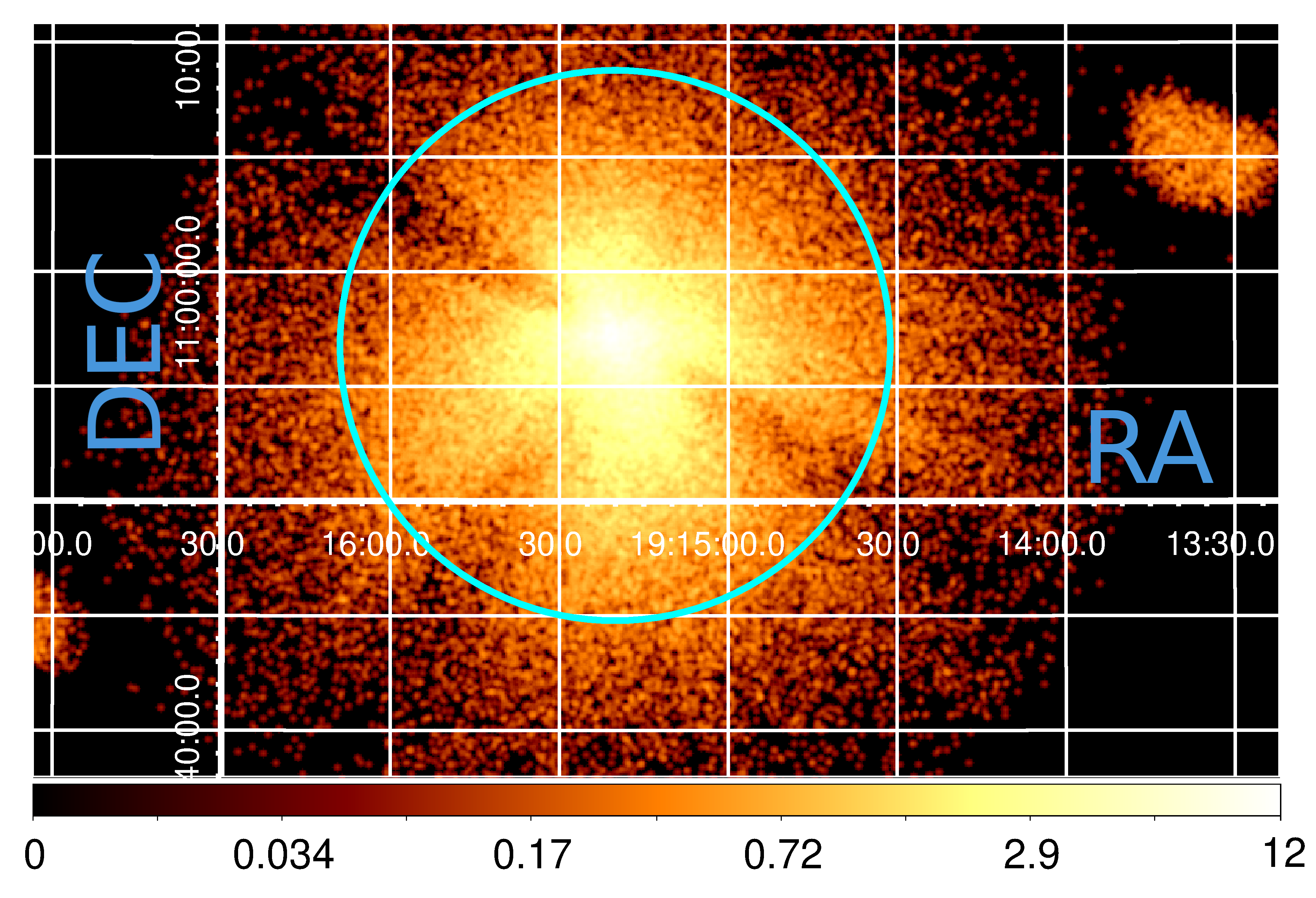
Figure 1: SXT image of the source GRS 1915$+$105 obtained with the PC mode data in $\omega$ class observation on MJD 57995.30 (Orbit 10394). The cyan circle corresponds to $12$ arcmin circular region, which is considered as the source region. The colormap denotes the intensity distribution of the source. See text for details.

2.2 Large Area X-ray Proportional Counter (LAXPC)

LAXPC is a proportional counter consisting of three identical detectors LAXPC10, LAXPC20 and LAXPC30 having combined effective area of 6000 ${\rm cm}^{2}$, which operates in $3-80$ keV energy range (Yadav et al., 2016; Agrawal et al., 2017; Antia et al., 2017). All the three LAXPC detectors have a temporal resolution of $10~{}\mu s$ that offers rich timing analysis compared to SXT. We use LAXPC level-1 data in event analysis mode available in AstroSat public archive³ for timing as well as spectral analyses. The details of LAXPC data extraction procedure and analysis methods are mentioned in Sreehari et al. (2019); Sreehari et al. (2020). The software LaxpcSoftv3.4(Antia et al., 2017), released on June 14, 2021 is used to process the level-1 data to level-2 data. We extract data from the top layer of the detector and consider only single events in our analysis. Further, we choose the background models, which are generated closest to the observation dates. While doing data extraction, LAXPC instrument response files are generated following Antia et al. (2017). The software generates the Good Time Interval (GTI) of the data consisting of the observation’s time information excluding the data gap due to Earth occultation and South Atlantic Anomaly (SAA). The longest continuous observation in each orbit is considered in the present analysis (see Table 1). Background subtracted LAXPC10 and LAXPC20 combined light curve of $1$ s time resolution in different energy ranges are generated by choosing the corresponding LAXPC channels using the standard routine of the software. It may be noted that we extract the source spectra from LAXPC20 data only as it’s gain remain stable throughout the entire observational period (Antia et al., 2021).

Table 2: Details of the best fitted PDS parameters from LAXPC observations of GRS 1915$+$105 in $3-60$ keV energy range in different variability classes. Results are obtained with combined data from LAXPC10 and LAXPC20. CO and L_i ($i=1,2,3,4$) denote the constant and multiple Lorentzians used to obtain the best fit. $\sigma$ denotes the significance of HFQPOs. $\rm HFQPO_{\rm rms}\%$ and $\rm Total_{\rm rms}\%$ represent the rms percentage of the HFQPO feature and the entire PDS. The centroid frequency (LC), FWHM (LW) and normalization (LN) of the detected HFQPOs are highlighted in bold font. All the errors are computed with 68% confidence level. See text for details.

	Model Parameters							Estimated Parameters
MJD (Orbit)	CO ($10^{-4}$)		$\rm L_{1}$	$\rm L_{2}$	$\rm L_{3}$	$\rm L_{4}$	$\chi^{2}/dof$	$\sigma$	$\rm HFQPO_{\rm rms}\%$	$\rm Total_{\rm rms}\%$	Class
		LC	0.0	0.0	$5.05_{-0.07}^{+0.05}$	$-$
57451.89 (2351)†	$1.58_{-0.01}^{+0.01}$	LW	$5.47_{-0.43}^{+0.57}$	$0.90_{-0.11}^{+0.14}$	$1.09_{-0.12}^{+0.23}$	$-$	$170/229$	$-$	$-$	$19.78\pm 6.78$	$\theta$
		LN	$0.0034_{-0.0007}^{+0.0007}$	$0.033_{-0.004}^{+0.004}$	$0.0010_{-0.0001}^{+0.0001}$	$-$
		LC	0.0	0.0	$3.25_{-0.01}^{+0.02}$	$6.11_{-0.11}^{+0.08}$
57452.82 (2365)†	$1.34_{-0.01}^{+0.01}$	LW	$3.94_{-0.49}^{+0.53}$	$0.85_{-0.21}^{+0.24}$	$0.44_{-0.01}^{+0.03}$	$2.36_{-0.31}^{+0.38}$	$168/232$	$-$	$-$	$17.71\pm 3.59$	$\chi$
		LN	$0.0037_{-0.0007}^{+0.0008}$	$0.0055_{-0.0008}^{+0.0007}$	$0.019_{-0.001}^{+0.002}$	$0.00077_{-0.00004}^{+0.00005}$
		LC	0.0	0.0	$6.19_{-0.16}^{+0.14}$	$-$
57453.35 (2373)†	$1.53_{-0.01}^{+0.01}$	LW	$7.87_{-1.81}^{+3.23}$	$1.37_{-0.18}^{+0.19}$	$1.75_{-0.39}^{+0.61}$	$-$	$137/235$	$-$	$-$	$20.09\pm 4.43$	$\theta$
		LN	$0.0011_{-0.0006}^{+0.0009}$	$0.0303_{-0.0031}^{+0.0036}$	$0.00046_{-0.00008}^{+0.00009}$	$-$
		LC	0.0	$1.71_{-0.21}^{+0.20}$	$\textbf{71.52}_{-0.29}^{+0.36}$	$-$
57504.02 (3124)	$1.86_{-0.01}^{+0.01}$	LW	$0.26_{-0.03}^{+0.04}$	$2.71_{-0.22}^{+0.23}$	$\textbf{1.25}_{-0.55}^{+0.62}$	$-$	$151/233$	$3.67$	$1.48\pm 0.36$	$21.03\pm 4.12$	$\omega$
		LN	$0.21_{-0.04}^{+0.05}$	$0.00097_{-0.00013}^{+0.00016}$	$\textbf{0.00011}_{-0.00003}^{+0.00004}$	$-$
		LC	0.0	0.0	$0.75_{-0.05}^{+0.06}$	$2.73_{-0.18}^{+0.21}$
57552.56 (3841)†	$1.39_{-0.01}^{+0.01}$	LW	$8.45_{-2.25}^{+1.84}$	$0.33_{-0.05}^{+0.06}$	$0.77_{-0.11}^{+0.14}$	$4.05_{-1.24}^{+0.98}$	$165/231$	$-$	$-$	$7.64\pm 2.18$	$\delta$
		LN	$0.00004_{-0.00001}^{+0.00001}$	$0.012_{-0.001}^{+0.002}$	$0.0014_{-0.0002}^{+0.0003}$	$0.00023_{-0.00004}^{+0.00004}$
		LC	0.0	$1.62_{-0.20}^{+0.23}$	$0.83_{-0.05}^{+0.04}$	$\textbf{69.31}_{-0.16}^{+0.11}$
57553.88 (3860)	$1.36_{-0.01}^{+0.01}$	LW	$0.018_{-0.004}^{+0.005}$	$3.10_{-0.16}^{+0.19}$	$1.05_{-0.19}^{+0.24}$	$\textbf{1.39}_{-1.06}^{+0.94}$	$134/228$	$2.75$	$1.54\pm 0.48$	$9.69\pm 2.23$	$\delta$
		LN	$0.29_{-0.02}^{+0.03}$	$0.0012_{-0.0003}^{+0.0003}$	$0.0021_{-0.0003}^{+0.0003}$	$\textbf{0.00011}_{-0.00004}^{+0.00004}$
		LC	0.0	${0.0}$	${3.59_{-0.34}^{+0.32}}$	${3.35_{-0.28}^{+0.39}}$
57689.10 (5862)†	${1.72_{-0.01}^{+0.01}}$	LW	${0.023_{-0.002}^{+0.001}}$	${1.34_{-0.14}^{+0.15}}$	${6.41_{-0.46}^{+0.49}}$	${0.98_{-0.23}^{+0.26}}$	${129/231}$	$-$	$-$	${26.30\pm 6.12}$	${\beta}$
		LN	${5.05_{-1.21}^{+1.45}}$	${0.013_{-0.002}^{+0.002}}$	${0.00071_{-0.00008}^{+0.00008}}$	${0.0012_{-0.0003}^{+0.0003}}$
		LC	0.0	0.0	$1.73_{-0.26}^{+0.33}$	$-$
57705.22 (6102)†	$1.37_{-0.01}^{+0.01}$	LW	$1.68_{-0.61}^{+0.71}$	$0.06_{-0.01}^{+0.02}$	$4.21_{-0.16}^{+0.15}$	$-$	$154/231$	$-$	$-$	$11.68\pm 2.71$	$\delta$
		LN	$0.0019_{-0.0003}^{+0.0006}$	$0.16_{-0.03}^{+0.08}$	$0.00092_{-0.00023}^{+0.00021}$	$-$
		LC	0.0	0.0	$5.14_{-0.02}^{+0.04}$	$10.33_{-0.21}^{+0.18}$
57891.88 (8863)†	$1.48_{-0.01}^{+0.01}$	LW	$13.47_{-1.66}^{+1.41}$	$0.18_{-0.03}^{+0.04}$	$1.15_{-0.11}^{+0.12}$	$3.47_{-0.89}^{+1.43}$	$183/232$	$-$	$-$	$27.38\pm 5.69$	$\rho\textprime$
		LN	$0.0011_{-0.0001}^{+0.0001}$	$0.42_{-0.12}^{+0.16}$	$0.0032_{-0.0002}^{+0.0003}$	$0.00042_{-0.00004}^{+0.00006}$
		LC	0.0	0.0	$5.74_{-0.05}^{+0.06}$	$10.63_{-0.23}^{+0.28}$
57892.74 (8876)†	$1.58_{-0.01}^{+0.01}$	LW	$3.80_{-0.67}^{+0.81}$	$0.13_{-0.03}^{+0.05}$	$1.54_{-0.14}^{+0.15}$	$8.43_{-0.93}^{+1.18}$	$144/222$	$-$	$-$	$23.53\pm 2.70$	$\rho$
		LN	$0.0016_{-0.0003}^{+0.0004}$	$0.71_{-0.18}^{+0.21}$	$0.0019_{-0.0001}^{+0.0002}$	$0.00043_{-0.00002}^{+0.00005}$
		LC	0.0	$-$	$-$	$-$
57943.69 (9629)†	$1.52_{-0.01}^{+0.01}$	LW	$0.14_{-0.01}^{+0.02}$	$-$	$-$	$-$	$149/239$	$-$	$-$	$35.49\pm 5.35$	$\kappa$
		LN	$1.26_{-0.24}^{+0.28}$	$-$	$-$	$-$
		LC	0.0	0.0	$\textbf{ {71.55}}_{-0.96}^{+0.96}$	$-$
57943.69 (9633)	$1.59_{-0.01}^{+0.01}$	LW	${0.13_{-0.01}^{+0.01}}$	${2.21_{-0.13}^{+0.15}}$	$\textbf{ {5.67}}_{-2.17}^{+2.76}$	$-$	${172/234}$	${3.71}$	${2.14\pm 0.50}$	$38.32\pm 6.67$	$\kappa$
		LN	${1.36_{-0.21}^{+0.24}}$	${0.016_{-0.002}^{+0.002}}$	$\textbf{0.000052}_{-0.000014}^{+0.000019}$	$-$
		LC	0.0	$\textbf{69.76}_{-0.74}^{+0.89}$	$-$	$-$
57946.10 (9666)	$1.55_{-0.01}^{+0.01}$	LW	$0.17_{-0.01}^{+0.02}$	$\textbf{5.01}_{-2.29}^{+2.93}$	$-$	$-$	$146/237$	${3.27}$	$2.55\pm 0.71$	$37.28\pm 6.31$	$\kappa$
		LN	$1.12_{-0.22}^{+0.26}$	$\textbf{0.000085}_{-0.000026}^{+0.000042}$	$-$	$-$
		LC	0.0	$6.79_{-1.05}^{+1.38}$	$\textbf{70.45}_{-0.53}^{+0.54}$	$-$
57946.34 (9670)	$1.67_{-0.01}^{+0.01}$	LW	$0.13_{-0.01}^{+0.01}$	$7.43_{-1.98}^{+1.69}$	$\textbf{4.67}_{-1.07}^{+1.56}$	$-$	$142/234$	${5.06}$	$2.49\pm 0.37$	$37.98\pm 5.35$	$\kappa$
		LN	$1.55_{-0.22}^{+0.25}$	$0.000078_{-0.000014}^{+0.000021}$	$\textbf{0.000086}_{-0.000017}^{+0.000018}$	$-$
		LC	0.0	$-$	$-$	$-$
57961.39 (9891)†	$5.46_{-0.01}^{+0.01}$	LW	$0.29_{-0.02}^{+0.04}$	$-$	$-$	$-$	$147/240$	$-$	$-$	$31.51\pm 4.35$	$\kappa$
		LN	$0.44_{-0.08}^{+0.12}$	$-$	$-$	$-$
		LC	0.0	0.0	$2.14_{-0.42}^{+0.48}$	$\textbf{71.68}_{-0.75}^{+0.84}$
57961.39 (9894)	$1.57_{-0.01}^{+0.01}$	LW	$2.14_{-0.01}^{+0.02}$	$0.09_{-0.02}^{+0.03}$	$1.25_{-0.31}^{+0.36}$	$\textbf{4.70}_{-2.21}^{+2.60}$	$156/232$	${3.43}$	$2.28\pm 0.63$	$42.31\pm 8.66$	$\kappa$
		LN	$0.04_{-0.01}^{+0.01}$	$1.70_{-0.53}^{+0.84}$	$0.0042_{-0.0011}^{+0.0011}$	$\textbf{0.000072}_{-0.000021}^{+0.000038}$
		LC	0.0	${0.72_{-0.01}^{+0.02}}$	$\textbf{70.47}_{-0.65}^{+0.69}$	$-$
57961.59 (9895)	$2.11_{-0.01}^{+0.01}$	LW	${0.13_{-0.01}^{+0.02}}$	${4.01_{-0.62}^{+0.66}}$	$\textbf{3.86}_{-1.32}^{+1.69}$	$-$	${171/234}$	${4.40}$	$1.98\pm 0.41$	${39.38\pm 7.30}$	$\kappa$
		LN	${1.59_{-0.28}^{+0.36}}$	${0.00105_{-0.00033}^{+0.00069}}$	$\textbf{0.000066}_{-0.000015}^{+0.000017}$	$-$
		LC	0.0	$0.32_{-0.02}^{+0.04}$	$6.79_{-0.24}^{+0.34}$	$\textbf{68.14}_{-0.61}^{+0.65}$
57995.30 (10394)	$2.06_{-0.01}^{+0.01}$	LW	${0.08_{-0.01}^{+0.02}}$	$0.61_{-0.02}^{+0.03}$	$2.46_{-1.10}^{+0.91}$	$\textbf{5.42}_{-1.11}^{+1.49}$	${165/231}$	${5.55}$	$2.25\pm 0.31$	$34.27\pm 9.76$	$\omega$
		LN	${1.23_{-0.39}^{+0.59}}$	$0.05_{-0.01}^{+0.01}$	$0.00012_{-0.00003}^{+0.00004}$	$\textbf{0.000061}_{-0.000011}^{+0.000012}$
		LC	0.0	$0.11_{-0.03}^{+0.02}$	$\textbf{70.01}_{-0.49}^{+0.56}$	$-$
57996.46 (10411)	$1.75_{-0.01}^{+0.01}$	LW	$0.03_{-0.01}^{+0.01}$	$0.57_{-0.05}^{+0.07}$	$\textbf{5.96}_{-0.99}^{+1.22}$	$-$	$193/234$	${7.01}$	$2.66\pm 0.29$	$26.45\pm 7.47$	$\omega$
		LN	$1.75_{-0.23}^{+0.44}$	$0.08_{-0.01}^{+0.01}$	$\textbf{0.000077}_{-0.000011}^{+0.000012}$	$-$
		LC	0.0	${1.89_{-0.31}^{+0.23}}$	$\textbf{72.22}_{-0.39}^{+0.49}$	$-$
58007.80 (10579)	$1.83_{-0.01}^{+0.01}$	LW	${0.25_{-0.03}^{+0.05}}$	${3.04_{-0.40}^{+0.42}}$	$\textbf{2.25}_{-1.48}^{+0.77}$	$-$	${128/234}$	${4.95}$	$1.86\pm 0.37$	$19.01\pm 3.66$	$\omega$
		LN	${0.18_{-0.03}^{+0.07}}$	${0.00068_{-0.00009}^{+0.00011}}$	$\textbf{0.000099}_{-0.000020}^{+0.000032}$	$-$
		LC	0.0	0.0	$2.25_{-0.05}^{+0.06}$	$\textbf{72.32}_{-0.21}^{+0.23}$
58008.08 (10583)	$1.37_{-0.01}^{+0.01}$	LW	$9.71_{-2.66}^{+4.19}$	$0.27_{-0.03}^{+0.03}$	$1.52_{-0.21}^{+0.23}$	$\textbf{3.61}_{-0.45}^{+0.48}$	$133/231$	${11.00}$	$2.46\pm 0.19$	$12.98\pm 3.72$	$\gamma$
		LN	$0.00021_{-0.00009}^{+0.00016}$	$0.062_{-0.011}^{+0.013}$	$0.0010_{-0.0001}^{+0.0001}$	$\textbf{0.00011}_{-0.00001}^{+0.00001}$
		LC	0.0	0.0	$0.61_{-0.02}^{+0.04}$	$-$
58046.36 (11154)†	$1.36_{-0.01}^{+0.01}$	LW	$4.66_{-0.32}^{+0.32}$	$0.21_{-0.04}^{+0.05}$	$0.43_{-0.06}^{+0.09}$	$-$	$166/234$	$-$	$-$	$7.91\pm 1.77$	$\delta$
		LN	$0.00086_{-0.00009}^{+0.00011}$	$0.013_{-0.003}^{+0.004}$	$0.0018_{-0.0002}^{+0.0003}$	$-$
		LC	0.0	0.0	${3.26_{-0.02}^{+0.02}}$	${6.32_{-0.06}^{+0.07}}$
58209.13 (13559)†	${1.43_{-0.01}^{+0.01}}$	LW	${6.18_{-0.35}^{+0.42}}$	${0.84_{-0.11}^{+0.13}}$	${0.64_{-0.04}^{+0.04}}$	${1.24_{-0.21}^{+0.23}}$	${171/232}$	$-$	$-$	${24.02\pm 4.23}$	${\chi}$
		LN	${0.0059_{-0.0008}^{+0.0006}}$	${0.018_{-0.002}^{+0.002}}$	${0.016_{-0.001}^{+0.001}}$	${0.00104_{-0.00011}^{+0.00012}}$
		LC	0.0	0.0	${2.20_{-0.01}^{+0.01}}$	${4.42_{-0.03}^{+0.03}}$
58565.82 (18839)†	${1.52_{-0.01}^{+0.01}}$	LW	${7.76_{-0.81}^{+1.29}}$	${0.57_{-0.15}^{+0.27}}$	${0.15_{-0.01}^{+0.03}}$	${0.39_{-0.09}^{+0.11}}$	${130/232}$	$-$	$-$	${21.14\pm 5.13}$	${\chi}$
		LN	${0.0045_{-0.0009}^{+0.0007}}$	${0.014_{-0.002}^{+0.003}}$	${0.031_{-0.003}^{+0.004}}$	${0.0048_{-0.0008}^{+0.0009}}$

• ^† Non-detection of HFQPO.

3 Timing Analysis and Results

3.1 Variability Classes and Color-Color Diagram (CCD)

We generate $1$ s binned light curve in the energy range $3-60$ keV, after combining the data from LAXPC10 and LAXPC20 while studying the structured variability in different classes. Following Agrawal et al. (2018); Sreehari et al. (2019); Sreehari et al. (2020), we correct the dead-time effect in all the light curves and calculate the average incident and detected count rates in $3-60$ keV energy range as tabulated in Table 1. The light curves are generated in $3-6$ keV, $6-15$ keV and $15-60$ keV energy ranges to plot the CCDs. We define the soft color and hard color following Sreehari et al. (2020) as ${\rm HR1}=B/A$ and ${\rm HR2}=C/A$, where $A$, $B$ and $C$ are the photon count rates in $3-6$ keV, $6-15$ keV and $15-60$ keV energy bands, respectively. The CCDs are obtained by plotting HR1 against HR2. It may be noted that the combined LAXPC10 and LAXPC20 background count rate ($\sim 225$ cts/s) is negligible ($\sim 2.5\%$) compared to the combined source count rate ($\sim 10000$ cts/s). Accordingly, we incorporate the background correction while carrying out the color-color and spectral analyses. However, power spectra are generated without background correction of light curves.

Following the classification scheme of Belloni et al. (2000), the light curves and CCDs indicate the presence of seven ‘softer’ variability classes as $\theta$, $\beta$, $\delta$, $\rho$, $\kappa$, $\omega$ and $\gamma$ with an additional variant ($\rho\textprime$) of $\rho$ class (Athulya et al., 2021), and one ‘harder’ variability class ($\chi$). The hardness ratios $HR1$ and $HR2$ for each class are tabulated in Table 1. It is clearly seen that the soft color $HR1$ and the hard color $HR2$ are generally less than $0.9$ and $0.1$, respectively, which imply the ‘softer’ variability classes. In Fig. 2, we present background subtracted and dead-time corrected LAXPC light curves of eight different variability classes ($\theta$, $\beta$, $\delta$, $\rho$, $\kappa$, $\omega$, $\gamma$ and $\chi$) with the CCD at the top-left inset of each panel. Different structured variability patterns along with the variations in the CCDs are observed in various classes.

During the AstroSat campaign, the source was initially observed in $\theta$ variability class (see Banerjee et al., 2021), where the count rate went up to $20$ kcts/s and both colors are softened as observed in the CCD. Further, the source was found in $\omega$, $\delta$ and $\beta$ variability classes (see Table 1.) Subsequently, the source was found in a variability class $\rho$ on MJD 57892.74. In this period, we see a ‘flare’ like nature in the light curve, and in the CCD, the points are distributed more towards the harder range. Next, the source displayed $\kappa$ class variability, in which the count rates were high as 15 kcts/s and multiple ‘dips’ (low counts) of few tens to hundred seconds of duration are observed. In addition, small duration ($\sim$ few seconds) ‘non-dips’ (high counts) are also present between the two ‘dips’. The CCD shows a uniform C-shaped distribution of points. In $\omega$ class, the duration of ‘non-dips’ between two ‘dips’ increases up to a few hundred of seconds, and the CCD shows a similar pattern as observed in $\kappa$ class. In $\gamma$ class, the long duration ‘dips’ are absent instead of small ‘dips’ with a few seconds of duration are observed along with high counts. A diagonally elongated distribution of points is found in the CCD. Finally, the source was found in ‘harder’ variability class ($\chi$) with count rate less than $1.5$ kcts/s (Athulya et al., 2021). In each panel of Fig. 2, we show the SXT light curves of the same observations in the energy range of $0.5-7$ keV at the top-middle inset. Similar structured variabilities are also observed in SXT light curves as seen in LAXPC observations.

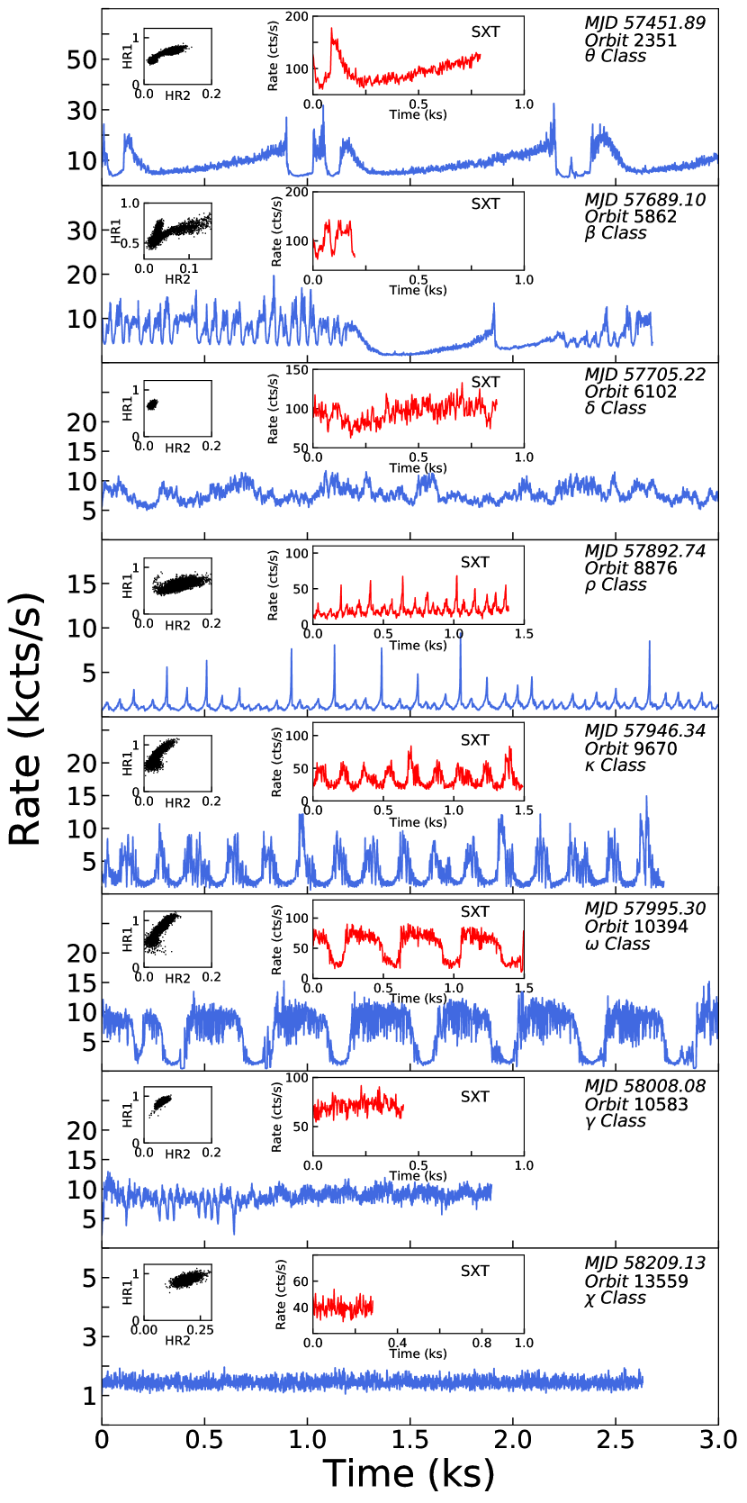
Figure 2: Background subtracted and dead-time corrected $1$ s binned light curves of GRS 1915+105 observed with AstroSat. Light curves corresponding to eight different variability classes, namely $\theta$, $\beta$, $\delta$, $\rho$, $\kappa$, $\omega$, $\gamma$ and $\chi$ are depicted from top to bottom panels. Each light curve is obtained by combining LAXPC10 and LAXPC20 data in $3-60$ keV energy band. In every panel, the CCD and the SXT light curves ($0.5-7$ keV) are also shown at the top-left and top-middle insets, respectively. See text for details.

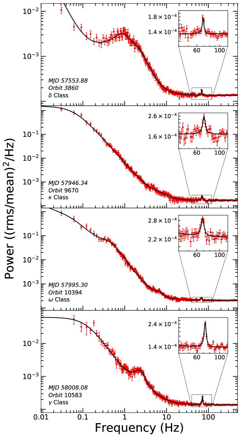
Figure 3: Power density spectra of four different variability classes in the presence of HFQPOs. Each PDS is obtained in $3-60$ keV energy range by combining LAXPC10 and LAXPC20 observations. In each panel, variability classes are marked, and the detected HFQPO features (zoomed view) are shown in the inset. See text for details.

3.2 Static Power Spectra

We generate light curves of $1$ ms resolution corresponding to each variability class with combined data from LAXPC10 and LAXPC20. We generate a power density spectrum (PDS) for each observation considering Nyquist frequency of $500$ Hz with these light curves. We choose $32768$ bins per interval for generating the respective PDS, which are further averaged to obtain the final PDS. A geometric binning factor of $1.03$ is used for the power spectral analysis. Finally, the dead-time corrected power spectra are obtained following Agrawal et al. (2018); Sreehari et al. (2019); Sreehari et al. (2020).

Each PDS (in units of $\rm(rms/mean)^{2}/Hz$) is then modelled using multiple Lorentzians and a constant component in the wide frequency range of $0.01-500$ Hz. Each Lorentzian is represented by three parameters, namely centroid (LC), width (LW), and normalization (LN). In Fig. 3, we present the model fitted PDS of $\delta$, $\kappa$, $\omega$ and $\gamma$ variability classes with the detected HFQPO feature as depicted in the inset of each panel. The variability class and the observation details are marked in each panel. First, we begin with the modeling of the power spectrum of $\gamma$ class observation using the model combination of a constant and four Lorentzians. Initially, two zero centroid Lorentzians and one Lorentzian with centroid frequency at 2.25 Hz along with a constant component are used to fit the entire PDS. The fit is resulted in a $\chi_{\rm red}^{2}$ of $310/234=1.32$. Further, to model the HFQPO feature, we include an additional Lorentzian with the centroid frequency of $\sim 72$ Hz. We emphasize that while modeling the entire PDS and estimating the errors associated with the model parameters, all the model parameters are kept free. The best fit is obtained with a $\chi_{\rm red}^{2}$ of $133/231=0.58$ (see also Sreehari et al., 2020). We follow the above procedure to fit the PDS in the presence of HFQPO features for $\delta$, $\kappa$ and $\omega$ classes, and the best fitted model parameters along with errors are tabulated in Table 2. In addition, we also note the presence of a broad feature in the PDS of $\delta$ and $\gamma$ class observations at $\sim 1$ Hz and $2$ Hz, respectively, which is absent in $\kappa$ and $\omega$ classes.

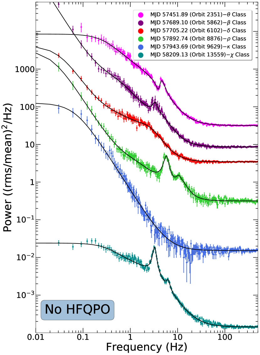
Figure 4: Power density spectra of six different observations in $3-60$ keV energy band, where HFQPO is absent. Magenta, purple, red, green, blue and darkcyan filled circles denote the PDS corresponding to $\theta$, $\beta$, $\delta$, $\rho$, $\kappa$ and $\chi$ classes, respectively. The power corresponding to $\theta$, $\beta$, $\delta$, $\rho$ and $\kappa$ class observations are scaled by multiplying $200000$, $50000$, $25000$, $2000$ and $100$ for the purpose of clarity. See text for details.

The presence of a HFQPO feature in the power spectra is determined by means of quality factor ($Q=LC/LW\geq 3$) and significance ($\sigma=LN/err_{\rm neg}\geq 3$), where $LC$, $LW$, $LN$ and $err_{\rm neg}$ denote the centroid frequency, width, normalization, and negative error of normalization of the fitted Lorentzian function (Sreehari et al., 2020, and references therein). Best fitted PDS of $\gamma$ class observation shows a strong signature of HFQPO feature of centroid frequency $72.32_{-0.21}^{+0.23}$ Hz with significance of $11\sigma$ as shown in the inset of the bottom panel of Fig. 3. We calculate the percentage rms of the HFQPO by taking the square root of the definite integral of Lorentzian function (van der Klis, 1988; Ribeiro et al., 2019; Sreehari et al., 2020, and references therein) with the HFQPO fitted parameters (i.e., LC, LW and LN) and obtain as $2.46\pm 0.19\%$. Further, we calculate the percentage rms of the entire PDS in the wide frequency range $0.01-500$ Hz and for $\gamma$ class observation, we obtain its value as $12.98\pm 3.72\%$. We detect $11$ such HFQPO features in four variability classes ($i.e.$, $\delta$, $\kappa$, $\omega$, $\gamma$) with centroid frequencies in the range of $68.14-72.32$ Hz, significance in the range of $2.75-11.0\sigma$ and the percentage rms in the range of $1.48-2.66$. The model fitted as well as estimated parameters of all observations are tabulated in Table 2.

To address the non-detection of the HFQPO features, we compute the percentage rms amplitude ($rms\%$) of the most significant peak near the observed HFQPO frequency for all the observations. We find the highest value of the percentage rms amplitude as $0.94\pm 0.15$ ($rms\%$ less than this value considered as ‘insignificant QPO rms’) for non-detection of HFQPO feature (see Table 3, Fig. 4 for PDS of $\kappa$ class). On contrary, we obtain the lowest value of $rms\%$ for the confirmed HFQPO detection as $1.48\pm 0.36$ in the power spectra. Accordingly, we identify thirteen observations in $\theta$, $\beta$, $\delta$, $\rho$, $\kappa$ and $\chi$ variability classes that do not exhibit the signature of HFQPO feature as presented in Table 3. Further, for reconfirmation (Belloni et al., 2001; Sreehari et al., 2020), we include one additional Lorentzian in the PDS of Orbit 9629 ($\kappa$ class, as an example) by freezing the centroid frequency at $69.76$ Hz and width at $5.01$ Hz, similar to the HFQPO characteristics obtained in Orbit 9666 ($\kappa$ class) having similar exposure. The significance of the best fitted Lorentzian feature is found to be $1.21$ at $1\sigma$ unit, which indicates the non-detection of HFQPO. All the model fitted parameters of the power spectra are presented in Table 2. In Fig. 4, we show the model fitted PDS corresponding to $\theta$, $\beta$, $\delta$, $\rho$, $\kappa$ and $\chi$ classes, modelled with Lorentzians and a constant. Note that in wide frequency band, the power spectra of $\delta$ class observation (Orbit 6102) shows a bump like feature near $2$ Hz, whereas the PDS corresponding to $\kappa$ class (Orbit 9629) is completely featureless. We find a strong Type-C LFQPO at $\sim 5.05$ Hz, $\sim 5.74$ Hz and $\sim 3.2$ Hz for $\theta$, $\rho$ and $\chi$ classes, respectively, whereas LFQPO feature at $\sim 3.35$ Hz is found broader for $\beta$ variability class. Here, we avoid the discussion on LFQPOs as it is beyond the scope of the present work.

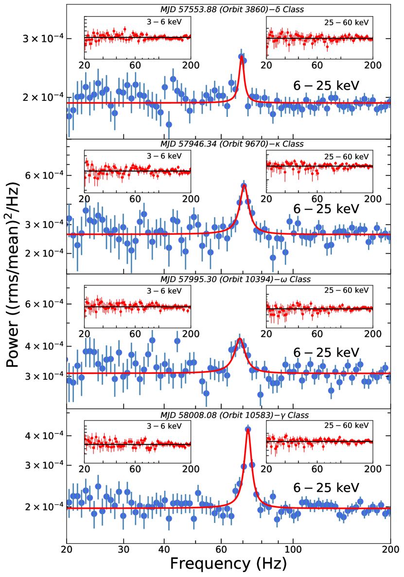
Figure 5: Energy dependent power density spectra depicted in $20-200$ Hz frequency range. PDS corresponding to $\delta$, $\kappa$, $\omega$ and $\gamma$ class observations are presented in sequence from top to bottom panels. Energy ranges are marked in each panel including insets. The PDS corresponding to $3-6$ keV and $25-60$ keV energy ranges are modelled with a constant, whereas the PDS in $6-25$ keV energy range is modelled using a constant and a Lorentizian. See text for details.

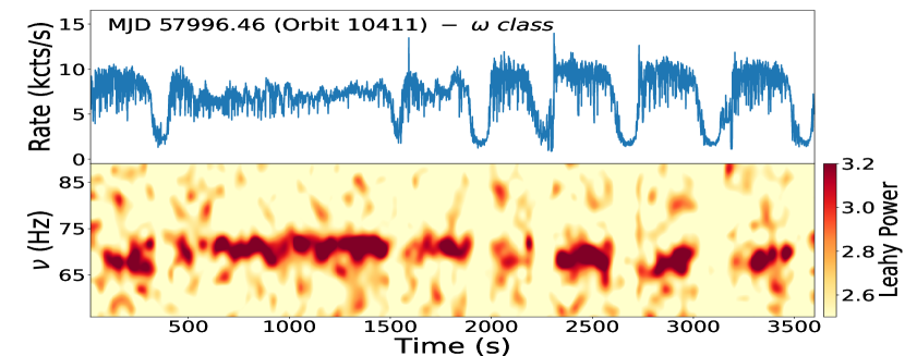
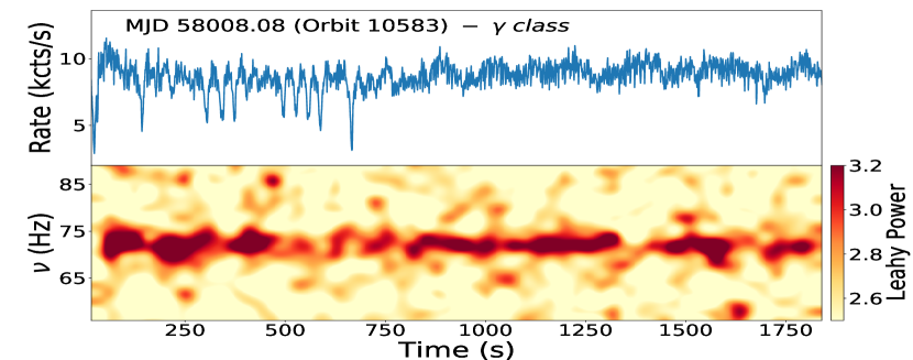
Figure 6: The light curves ($3-60$ keV) of $\omega$ and $\gamma$ classes are depicted in the top panels of each plot. In the bottom panels of each plot, the dynamical power spectra generated from the high resolution ($1$ ms) light curve are presented. Here, $32$ s segment size and $2$ Hz frequency bin are used to represent the dynamical power spectra. The obtained results are presented using color code, where colorbars are marked in the right of the bottom panels. See text for details.

3.3 Energy dependent Power Spectra

We study the energy dependent PDS for all the ‘softer’ variability classes to examine the HFQPO features. While doing so, we divide $3-60$ keV energy band into different energy intervals and search for HFQPO features following the same method as discussed in section 3.2. We find that for $\gamma$ class observation, the HFQPOs are present only in $6-25$ keV energy range with higher rms amplitude ($\sim 3.64\%$) and higher significance ($\sigma\sim 12$) at $1\sigma$ unit compared to that in $3-60$ keV energy band (see Table 2 and 3). What is more is that the PDS corresponding to $3-6$ keV and $25-60$ keV energy bands are found to be featureless (see Fig. 5) as the $rms\%$ corresponding to the most significant peak are obtained as $\sim 0.92$ and $\sim 0.74$, respectively. In addition, we model the PDS in $3-6$ keV and $25-60$ keV energy bands using Lorentzian function with centroid fixed at $\sim 72.32$ Hz for $\gamma$ class (see Belloni et al., 2001; Sreehari et al., 2020). The highest values of the significance of the fitted Lorentzian are found to be $1.63\sigma$ and $0.7\sigma$ in $3-6$ keV and $25-60$ keV energy bands, respectively. These results clearly indicate the non-detection of HFQPO feature as the percentage rms are insignificant. We follow same methodology for all the observations under consideration and find that the prominent HFQPO features are present only in $6-25$ keV energy range (see Fig. 5 and Table 3). In Fig. 5, HFQPO feature is shown in each panel along with the non-detection cases at the insets. Moreover, we carry out the wide-band spectral analysis to understand the emission mechanisms that possibly manifest the HFQPO signatures (see section 4).

3.4 Dynamical Power Spectra

The power spectra in different variability classes reveal that HFQPOs are not persistent but rather sporadic in nature. Therefore, we examine the dynamic nature of the power spectrum, where we search for HFQPO in each segment of duration $32$ s of the entire light curve of $1$ ms resolution. The Leahy power spectrum (Leahy et al., 1983) for each segment of the light curve is computed and plotted as a vertical slice corresponding to each time bin using the stingray package (Huppenkothen et al., 2019). The frequency bin size is chosen as $2$ Hz. We use bicubic interpolation (Huppenkothen et al., 2019) to improve clarity and smoothen the dynamic power spectrum. The power corresponding to each frequency is color coded such that yellow indicates minimum power and red indicates maximum power as shown in the colorbar of Fig. 6.

In the left side of Fig. 6, we present the light curve (top panel) of Orbit 10411, generated by combining LAXPC10 and LAXPC20 light curves along with the corresponding dynamic power spectrum (bottom panel). The light curve corresponds to the $\omega$ class variability (see Fig. 2). It is observed that the power at frequencies around $70$ Hz is significant during ‘non-dips’ (high counts) and is insignificant during the ‘dips’ (low counts). The percentage rms amplitude of the HFQPO during high counts and low counts are obtained as $2.38\pm 0.29$ and $0.67\pm 0.18$ for $\omega$ class observation, respectively. This clearly suggests that the HFQPO of frequencies around $70$ Hz are generated when the count rate is high. We also observe similar behavior during $\gamma$ class observation. From the right side of Fig. 6, it is evident that the source emits at high count rate of about $9000$ cts/s throughout the observation. As a result, HFQPO is seen to be present in almost every $32$ s interval, although its power amplitude reduces during the narrow dips ($500-700$ s) present in the light curve. Overall, by analyzing the dynamic PDS, we infer that within the ‘softer’ variability classes ($\kappa$, $\omega$ and $\gamma$), high count rate (non-dips) seems to be associated with the generation of HFQPO features as illustrated in Appendix A.

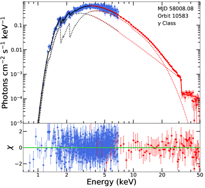
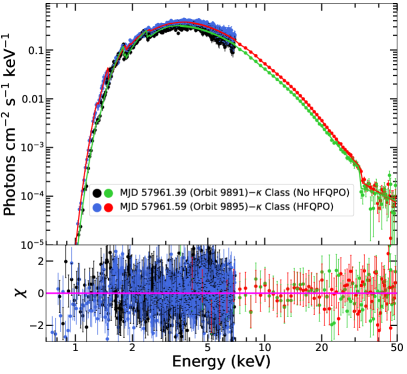
Figure 7: Unfolded wide-band ($0.7-50$ keV) energy spectra of the source GRS $1915+105$. The spectra are modelled with Tbabs$\times$(smedge$\times$nthComp + powerlaw)$\times$constant. The spectra of $\gamma$ class observation on MJD 58008.08 (Orbit 10583) is presented in the left. Two best fitted spectra of $\kappa$ class variabilities without (MJD 57961.39; Orbit 9891) and with (MJD 57961.59; Orbit 9895) HFQPO are depicted in the right. The bottom panels of each plot show the residuals in units of $\sigma$. See text for details.

Table 3: Estimated percentage rms amplitudes of HFQPOs in different energy bands. All the errors are computed with 68% confidence level. See text for more details.

	HFQPO rms amplitude (%)			Non-detection of HFQPO	Detection of HFQPO
MJD (Orbit)	energy band	energy band	energy band	rms%	HFQPO rms%	Class
	($3-6$ keV)	($6-25$ keV)	($25-60$ keV)	($3-60$ keV)	($3-60$ keV)
57451.89 (2351)†	$-$	$-$	$-$	$0.54\pm 0.23$	$-$	$\theta$
57452.82 (2365)†	$-$	$-$	$-$	$0.38\pm 0.11$	$-$	$\chi$
57453.35 (2373)†	$-$	$-$	$-$	$0.44\pm 0.16$	$-$	$\theta$
57504.02 (3124)	$0.39\pm 0.11$	$2.33\pm 0.25$	$0.81\pm 0.32$	$-$	$1.48\pm 0.36$	$\omega$
57552.56 (3841)†	$-$	$-$	$-$	$0.61\pm 0.23$	$-$	$\delta$
57553.88 (3860)	$0.79\pm 0.28$	$2.12\pm 0.22$	$0.88\pm 0.25$	$-$	$1.54\pm 0.48$	$\delta$
57689.10 (5862)†	$-$	$-$	$-$	$0.16\pm 0.09$	$-$	$\beta$
57705.22 (6102)†	$-$	$-$	$-$	$0.86\pm 0.15$	$-$	$\delta$
57891.88 (8863)†	$-$	$-$	$-$	$0.23\pm 0.12$	$-$	$\rho\textprime$
57892.74 (8876)†	$-$	$-$	$-$	$0.77\pm 0.26$	$-$	$\rho$
57943.69 (9629)†	$-$	$-$	$-$	$0.94\pm 0.15$	$-$	$\kappa$
57943.69 (9633)	$0.38\pm 0.14$	$3.65\pm 0.31$	$0.56\pm 0.12$	$-$	$2.14\pm 0.50$	$\kappa$
57946.10 (9666)	$0.75\pm 0.18$	$3.34\pm 0.48$	$0.62\pm 0.21$	$-$	$2.55\pm 0.71$	$\kappa$
57946.34 (9670)	$0.83\pm 0.22$	$4.29\pm 0.54$	$0.71\pm 0.13$	$-$	$2.49\pm 0.37$	$\kappa$
57961.39 (9891)†	$-$	$-$	$-$	$0.82\pm 0.24$	$-$	$\kappa$
57961.39 (9894)	$0.79\pm 0.15$	$2.86\pm 0.29$	$0.77\pm 0.11$	$-$	$2.28\pm 0.63$	$\kappa$
57961.59 (9895)	$0.19\pm 0.07$	$3.12\pm 0.63$	$0.84\pm 0.33$	$-$	$1.98\pm 0.41$	$\kappa$
57995.30 (10394)	$0.72\pm 0.21$	$3.30\pm 0.55$	$0.67\pm 0.12$	$-$	$2.25\pm 0.31$	$\omega$
57996.46 (10411)	$0.84\pm 0.24$	$4.01\pm 0.37$	$0.81\pm 0.15$	$-$	$2.66\pm 0.29$	$\omega$
58007.80 (10579)	$0.68\pm 0.12$	$3.21\pm 0.42$	$0.89\pm 0.19$	$-$	$1.86\pm 0.37$	$\omega$
58008.08 (10583)	$0.92\pm 0.16$	$3.64\pm 0.24$	$0.74\pm 0.21$	$-$	$2.46\pm 0.19$	$\gamma$
58046.36 (11154)†	$-$	$-$	$-$	$0.42\pm 0.14$	$-$	$\delta$
58209.13 (13559)†	$-$	$-$	$-$	$0.76\pm 0.13$	$-$	$\chi$
58565.82 (18839)†	$-$	$-$	$-$	$0.69\pm 0.11$	$-$	$\chi$

• ^† Non-detection of HFQPO.

Table 4: Best fitted parameters of the wide-band ($0.7-50$ keV) energy spectra of GRS 1915$+$105 with the model Tbabs$\times$(smedge$\times$nthComp $+$ powerlaw)$\times$constant for different observations as mentioned in Table 1. In the table, $kT_{e}$ is the electron temperature in keV, $\Gamma_{\rm nth}$ is the nthComp photon index, $norm_{\rm nth}$ is the nthComp normalization. $\Gamma_{\rm PL}$ and $norm_{\rm PL}$ are the powerlaw photon index and normalization, respectively. $F_{\rm nth}$ and $F_{\rm PL}$ are the flux in erg cm^-2 s^-1 associated with nthComp and powerlaw components, respectively. $F_{\rm bol}$, $L_{\rm bol}$, $\tau$ and y-par are the bolometric flux, bolometric luminosity in units of $\%L_{\rm Edd}$, optical depth and Compton y-parameter, respectively. All the errors are computed with $90$ per cent confidence level. See text for details.

	Model fitted parameters						Estimated parameters
MJD (Orbit)	$kT_{e}$	$\Gamma_{\rm nth}$	$norm_{\rm nth}$	$\Gamma_{\rm PL}$	$norm_{\rm PL}$	$\chi_{\rm red}^{2}$	$F_{\rm nth}$	$F_{\rm PL}$	$F_{\rm bol}$	$L_{\rm bol}$	$\tau$	y-par	Class
	(keV)						($0.7-50$ keV)	($0.7-50$ keV)	($0.3-100$ keV) ⊞	( $\%L_{\rm Edd}$)
							($\tiny{10^{-8}}$ erg ${\rm cm}^{-2}{\rm s}^{-1}$)	($\tiny{10^{-8}}$ erg ${\rm cm}^{-2}{\rm s}^{-1}$)	($\tiny{10^{-8}}$ erg ${\rm cm}^{-2}{\rm s}^{-1}$)
57451.89 (2351)†	$3.66_{-0.12}^{+0.11}$	$2.89_{-0.05}^{+0.08}$	$34_{-2}^{+3}$	$2.85_{-0.07}^{+0.07}$	$42_{-3}^{+4}$	1.14	2.51	2.84	5.38	30	6	0.83$\pm$0.06	$\theta$
57452.82 (2365)†,¶	$23.92_{-4.72}^{+7.54}$	$2.57_{-0.03}^{+0.03}$	$18_{-1}^{+1}$	$-$	$-$	1.06	2.45	$-$	3.03	17	2	0.63$\pm$0.08	$\chi$
57453.35 (2373)†	$3.10_{-0.07}^{+0.08}$	$2.47_{-0.02}^{+0.03}$	$29_{-2}^{+4}$	$2.59_{-0.03}^{+0.03}$	$23_{-2}^{+2}$	1.08	2.85	3.14	6.05	34	7	1.29$\pm$0.04	$\theta$
57504.02 (3124)	$2.37_{-0.11}^{+0.12}$	$1.97_{-0.05}^{+0.06}$	$16_{-2}^{+3}$	$2.65_{-0.08}^{+0.09}$	$4_{-1}^{+2}$	1.18	4.46	0.44	5.06	28	12	2.47$\pm$0.21	$\omega$
57552.56 (3841)†	$1.94_{-0.05}^{+0.04}$	$1.83_{{-0.08}}^{+0.06}$	${16_{-4}^{+3}}$	$3.27_{{-0.06}}^{{+0.05}}$	${34_{-7}^{+6}}$	1.19	3.52	1.71	5.24	29	14	3.12$\pm$ 0.35	$\delta$
57553.88 (3860)	$2.53_{{-0.11}}^{{+0.10}}$	$2.08_{{-0.11}}^{{+0.09}}$	${19_{-5}^{+5}}$	$3.18_{{-0.04}}^{{+0.05}}$	${32_{-3}^{+4}}$	1.12	3.57	1.15	4.73	27	10	2.11$\pm$ 0.31	$\delta$
57689.10 (5862)†	$1.82_{-0.09}^{+0.11}$	$2.13_{-0.06}^{+0.06}$	$12_{-3}^{+4}$	$2.83_{-0.07}^{+0.07}$	$20_{-5}^{+4}$	1.11	1.64	1.91	3.85	22	12	2.06$\pm$0.16	$\beta$
57705.22 (6102)†	$1.93_{{-0.04}}^{{+0.06}}$	$1.90_{{-0.05}}^{{+0.05}}$	${15_{-2}^{+4}}$	$3.21_{{-0.03}}^{{+0.04}}$	${24_{-2}^{+3}}$	1.08	2.37	1.67	4.26	24	14	2.80$\pm$ 0.21	$\delta$
57891.88 (8863)†	10∗	$2.30_{{-0.02}}^{{+0.04}}$	${9_{-1}^{+2}}$	$-$	$-$	1.22	1.03	$-$	1.05	6	$-$	$-$	$\rho\textprime$
57892.74 (8876)†	10∗	$2.86_{{-0.07}}^{{+0.04}}$	${13_{-2}^{+3}}$	$-$	$-$	1.17	1.02	$-$	1.16	7	$-$	$-$	$\rho$
57943.69 (9629)†	$2.38_{{-0.06}}^{{+0.06}}$	$1.96_{{-0.07}}^{{+0.08}}$	${6_{-1}^{+1}}$	$2.73_{{-0.05}}^{{+0.05}}$	${2_{-1}^{+1}}$	1.02	1.04	0.59	1.65	9	12	2.51$\pm$ 0.29	$\kappa$
57943.69 (9633)	$2.36_{{-0.05}}^{{+0.06}}$	$2.11_{{-0.09}}^{{+0.07}}$	${7_{-2}^{+1}}$	$3.26_{{-0.03}}^{{+0.04}}$	${15_{-1}^{+3}}$	1.18	1.06	0.52	1.57	9	11	2.04$\pm$ 0.21	$\kappa$
57946.10 (9666)	$2.39_{{-0.08}}^{{+0.11}}$	$2.03_{{-0.05}}^{{+0.06}}$	${7_{-1}^{+2}}$	$3.13_{{-0.04}}^{{+0.04}}$	${13_{-2}^{+3}}$	1.03	1.21	0.54	1.76	10	11	2.27$\pm$ 0.19	$\kappa$
57946.34 (9670)	$2.50_{{-0.06}}^{{+0.07}}$	$2.06_{{-0.04}}^{{+0.04}}$	${7_{-1}^{+1}}$	$3.24_{{-0.03}}^{{+0.03}}$	${16_{-1}^{+1}}$	1.17	1.10	0.55	1.78	10	11	2.17$\pm$ 0.12	$\kappa$
57961.39 (9891)†	$2.48_{{-0.08}}^{{+0.09}}$	$1.97_{{-0.06}}^{{+0.06}}$	${7_{-1}^{+1}}$	$2.80_{{-0.06}}^{{+0.05}}$	${6_{-2}^{+1}}$	1.23	1.03	0.84	2.03	12	11	2.46$\pm$ 0.21	$\kappa$
57961.39 (9894)	$2.64_{{-0.07}}^{{+0.10}}$	$2.10_{{-0.05}}^{{+0.07}}$	${10_{-1}^{+1}}$	$3.05_{{-0.04}}^{{+0.05}}$	${14_{-1}^{+1}}$	1.12	1.52	0.83	2.48	14	10	2.04$\pm$ 0.19	$\kappa$
57961.59 (9895)	$2.77_{{-0.12}}^{{+0.11}}$	$2.23_{{-0.12}}^{{+0.07}}$	${16_{-2}^{+3}}$	$3.12_{{-0.05}}^{{+0.05}}$	${18_{-1}^{+1}}$	1.06	1.53	0.98	2.53	14	9	1.72$\pm$ 0.25	$\kappa$
57995.30 (10394)	$3.06_{{-0.08}}^{{+0.13}}$	$2.44_{{-0.08}}^{{+0.05}}$	${33_{-5}^{+4}}$	$3.12_{{-0.03}}^{{+0.04}}$	${26_{-2}^{+4}}$	1.06	1.74	1.37	3.23	18	8	1.33$\pm$ 0.12	$\omega$
57996.46 (10411)	$3.07_{{-0.11}}^{{+0.11}}$	$2.36_{{-0.05}}^{{+0.05}}$	${27_{-3}^{+3}}$	$3.13_{{-0.04}}^{{+0.04}}$	${24_{-1}^{+1}}$	1.17	1.94	1.36	3.43	19	8	1.46$\pm$ 0.08	$\omega$
58007.80 (10579)	$2.67_{{-0.11}}^{{+0.09}}$	$2.17_{{-0.11}}^{{+0.06}}$	${21_{-4}^{+3}}$	$3.10_{{-0.04}}^{{+0.03}}$	${26_{-1}^{+2}}$	0.98	2.24	1.31	3.85	22	9	1.86$\pm$ 0.14	$\omega$
58008.08 (10583)	$2.62_{{-0.12}}^{{+0.10}}$	$2.02_{{-0.07}}^{{+0.06}}$	${15_{-2}^{+2}}$	$3.00_{{-0.06}}^{{+0.05}}$	${21_{-3}^{+4}}$	1.08	2.49	1.37	4.16	23	11	2.27$\pm$ 0.22	$\gamma$
58046.36 (11154)†	$2.03_{{-0.06}}^{{+0.08}}$	$1.84_{{-0.05}}^{{+0.05}}$	${15_{-2}^{+3}}$	$2.99_{{-0.06}}^{{+0.07}}$	${14_{-1}^{+2}}$	1.25	3.36	1.68	5.12	29	14	3.05$\pm$ 0.24	$\delta$
58209.13 (13559)†,¶	20∗	$2.19_{-0.04}^{+0.04}$	$8_{-1}^{+1}$	$-$	$-$	0.93	2.21	$-$	2.34	13	$-$	$-$	$\chi$
58565.82 (18839)†,¶	20∗	$1.88_{-0.02}^{+0.02}$	$0.71_{-0.02}^{+0.03}$	$-$	$-$	1.03	0.51	$-$	0.53	3	$-$	$-$	$\chi$

• SXT response extends from $0.3$ keV. ^† No detection of HFQPO.

• Frozen at $10$ and $20$ keV, below this value the spectral fitting is affected yielding higher $\chi^{2}_{red}$.

• Modelled with diskbb and nthComp component. Inner disc temperature, $T_{in}\sim 0.25$ keV.

4 Spectral Analysis and results

For each variability class, we generate the corresponding wide-band energy spectra combining the SXT and LAXPC20 data. We consider $0.7-7$ keV energy range for SXT spectra, whereas LAXPC spectra are extracted in the energy range of $3-50$ keV (see Sreehari et al., 2019; Sreehari et al., 2020, for details). The dead-time corrections are applied to the LAXPC spectra while extracting with LaxpcSoftv3.4 software (Antia et al., 2017).

We model the wide-band energy spectra using XSPEC V12.10.1f in HEASOFT V6.26.1 to understand the radiative emission processes active around the source. While modelling the energy spectra, we consider a systematic error of 2$\%$ for both SXT and LAXPC data (Antia et al., 2017; Leahy & Chen, 2019; Sreehari et al., 2020). We use the gain fit command in XSPEC to take care of the instrumental features at $1.8$ keV and $2.2$ keV in SXT spectra. While applying gain fit, we allow the offset to vary and fix the slope at $1$. The hydrogen column density (nH) is kept fixed at $6\times 10^{22}$ atoms/cm² following Yadav et al. (2016); Sreehari et al. (2020).

To begin with, we adopt a model Tbabs$\times$nthComp$\times$constant to fit the wide-band energy spectrum of $\gamma$ class observation (Orbit 10583) for which the strongest HFQPO feature is seen in the PDS (bottom panel of Fig. 3). Here, the model Tbabs (Wilms et al., 2000) takes care of the galactic absorption between the source and the observer. The model nthComp (Zdziarski et al., 1996) represents the thermally Comptonized continuum. A constant parameter is used to account for the offset between the spectra from two different instruments, SXT and LAXPC. The obtained fit is yielded a poor reduced $\chi^{2}$ ($\chi_{\rm red}^{2}=\chi^{2}/dof$) of $2095/546=3.83$ as there are large residuals left at the higher energies beyond $30$ keV. Hence, we include a powerlaw along with one Xenon edge component at $32$ keV (Sreehari et al., 2019) to fit the high energy part of the spectrum. The Xenon edge is required for all the energy spectra to account for the instrumental absorption feature at $32-35$ keV. Also, one smedge component is used at $\sim 9$ keV to obtain the best fit. The model Tbabs$\times$(smedge$\times$nthComp $+$ powerlaw)$\times$constant provides statistically acceptable fit with $\chi_{\rm red}^{2}=\chi^{2}/dof$ of $563/533=1.08$. In the left side of Fig. 7, we present the best fitted unfolded energy spectrum of $\gamma$ class observation for representation.

The best fitted model parameters of the nthComp component for $\gamma$ class observation (Orbit 10583) are obtained as electron temperature $(kT_{e})=2.62^{+0.10}_{-0.12}$ keV, photon index $(\Gamma_{\rm nth})=2.02^{+0.06}_{-0.07}$ with normalization $(norm_{\rm nth})=15\pm 2$. The seed photon temperature ($kT_{\rm bb}$) is kept fixed at $0.1$ keV during the fitting. The best fitted value for the powerlaw photon index ($\Gamma_{\rm PL}$) is obtained as $\Gamma_{\rm PL}=3.00^{+0.05}_{-0.06}$ with powerlaw normalization $norm_{\rm PL}=21^{+4}_{-3}$. Following the same approach, we carry out the spectral modelling for all other observations of various variability classes ($i.e.$, $\theta$, $\beta$, $\delta$, $\rho$, $\kappa$, $\omega$, $\gamma$ and $\chi$) irrespective to the presence or absence of HFQPOs. The best fitted model parameters are tabulated in Table LABEL:table:Spectral_parameters. It is found that in all observations, the model Tbabs$\times$(smedge$\times$nthComp $+$ powerlaw)$\times$constant satisfactorily describes the energy spectra except for $\rho$ and $\chi$ class observations. For $\rho$ class, the acceptable fit is obtained without powerlaw component, whereas in $\chi$ class observation, an additional diskbb component is required along with nthComp. Note that we are unable to constrain the electron temperature for the observations of $\rho$, $\rho^{\prime}$ and two $\chi$ classes and hence we fix the electron temperature $kT_{e}=10$ keV and $20$ keV, respectively (see Table LABEL:table:Spectral_parameters). In the right side of Fig. 7, we present the wide-band energy spectra of two $\kappa$ class observations on MJD 57961.39 (Orbit 9891) and MJD 57961.59 (Orbit 9895) without and with HFQPO feature, respectively. We point out that the best fitted energy spectrum of orbit 9891 (without HFQPO) has a weak nthComp contribution ( $norm_{\rm nth}\sim 7$), whereas in orbit 9895 (with HFQPO), the nthComp contribution ( $norm_{\rm nth}\sim 16$) is relatively higher. We also find relatively high electron temperatures in those observations that ascertain the detection of HFQPOs except one observation in $\theta$ class (Orbit 2351).

Further, we estimate the flux in the energy range $0.7-50$ keV associated with different model components used for the spectral fitting. While doing so, the convolution model cflux in XSPEC is used. For $\gamma$ class observation, the fluxes associated with nthComp and powerlaw components are estimated as $2.49$ and $1.37$ in units of $10^{-8}$ erg ${\rm cm}^{-2}~{}{\rm s}^{-1}$, respectively (see Table LABEL:table:Spectral_parameters). We also calculate bolometric flux ($F_{\rm bol}$) in the energy range $0.3-100$ keV using the cflux model. Considering the mass ($M_{\rm BH}$) and the distance ($d$) of the source as $M_{\rm BH}=12.4M_{\odot}$ and $d=8.6$ kpc (Reid et al., 2014), we calculate the bolometric luminosity in units of Eddington luminosity ($L_{\rm Edd}$) as $L_{\rm bol}=F_{\rm bol}\times 4\pi d^{2}$. The luminosity is found to vary in the range of $3-34\%$ $L_{\rm Edd}$. The calculated flux values and bolometric luminosities for all the observations are given in Table LABEL:table:Spectral_parameters.

In order to understand the nature of the Comptonizing medium in the vicinity of the source, we calculate the optical depth ($\tau$) of the medium. Following Zdziarski et al. (1996); Chatterjee et al. (2021), the relation among the optical depth ($\tau$), nthComp spectral index ($\alpha=\Gamma_{\rm nth}-1$), and electron temperature ($kT_{e}$) is given by,

$$\alpha=\left[\frac{9}{4}+\frac{1}{\left(\nicefrac{{kT_{e}}}{{m_{e}c^{2}}}\right)\tau\left(1+\nicefrac{{\tau}}{{3}}\right)}\right]^{\nicefrac{\mathrm{1}}{\mathrm{2}}}-\frac{3}{2},$$

where $m_{e}$ is the electron mass, and $c$ refers to the speed of light. Using equation (1), the optical depth ($\tau$) is calculated and found in the range $2\lesssim\tau\lesssim 14$ for all the observations. This implies that an optically thick corona is present as a Comptonizing medium in the vicinity of the source. Moreover, we calculate the Compton y-parameter, which measures the degree of Compton up-scattering of soft photons in the underlying accretion flow by the Comptonizing medium. Following Agrawal et al. (2018); Chatterjee et al. (2021), the Compton y-parameter ($=4kT_{e}\tau^{2}/m_{e}c^{2}$) in the optically thick medium is found to be in the range of $0.63\pm 0.08~{}-~{}3.12\pm 0.35$. In Table LABEL:table:Spectral_parameters, we tabulate the obtained optical depth ($\tau$) and Compton y-parameter values for all the observations.

5 Spectro-temporal correlation

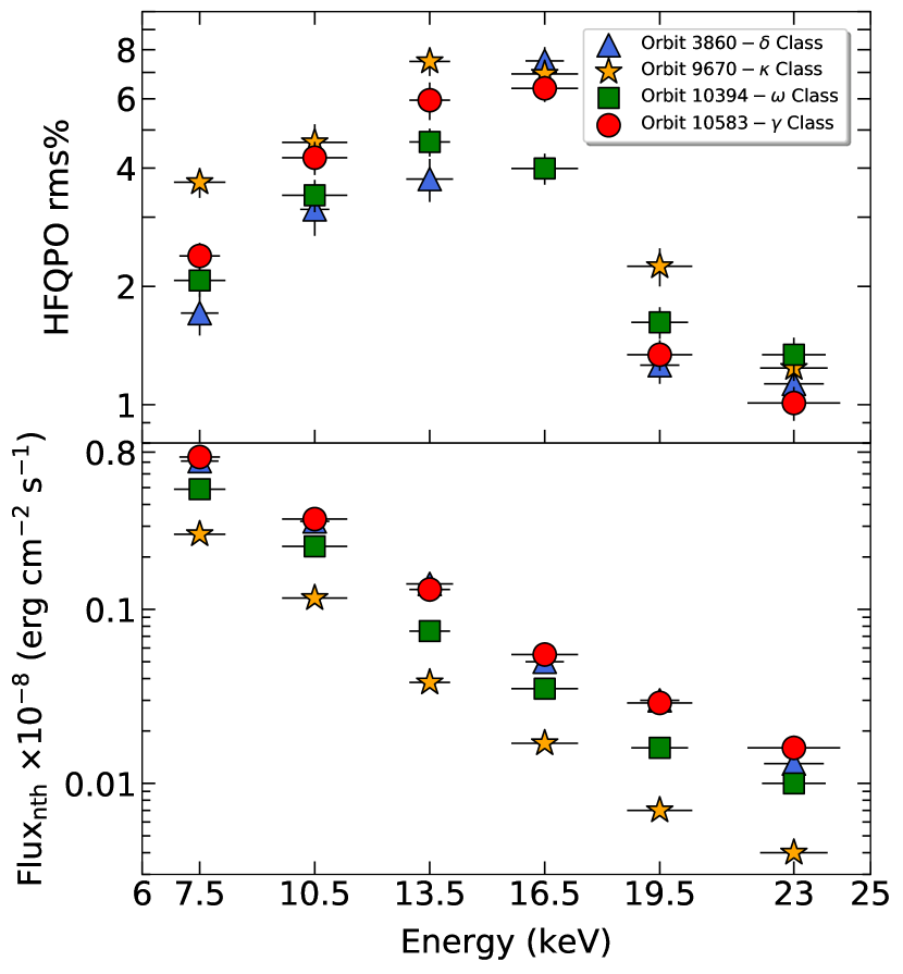
Figure 8: Top: Variation of percentage rms amplitudes ($rms\%$) of HFQPOs with energy for $\delta$, $\kappa$, $\omega$ and $\gamma$ variability classes. Bottom: Variation of nthComp flux with energy corresponding to the variability classes as marked in the inset of the top panel. See text for details.

In this section, we examine the spectro-temporal correlation of the observed properties in different variability classes of GRS 1915+105. While doing so, we consider four variability classes, namely $\delta$, $\kappa$, $\omega$ and $\gamma$, and study the variation of the percentage rms amplitude ($rms\%$) of HFQPO features as function of energy shown in the top panel of Fig. 8. The results corresponding to $\delta$, $\kappa$, $\omega$ and $\gamma$ classes are denoted by the filled triangles (blue), asterisks (yellow), squares (green) and circles (red), respectively. We find that HFQPO $rms\%$ increases with energy up to $\sim 17$ keV and then sharply decreases. Further, to correlate the evolution of $rms\%$ with the Comptonized flux ($i.e.$, nthComp), we present the variation of the estimated nthComp flux in the respective energy bands as shown in the bottom panel of Fig. 8. We notice that nthComp flux decreases with energy and it becomes negligible beyond $\sim 25$ keV ($\sim 2\%$ of the total nthComp flux in $3-60$ keV; see also Fig. 7).

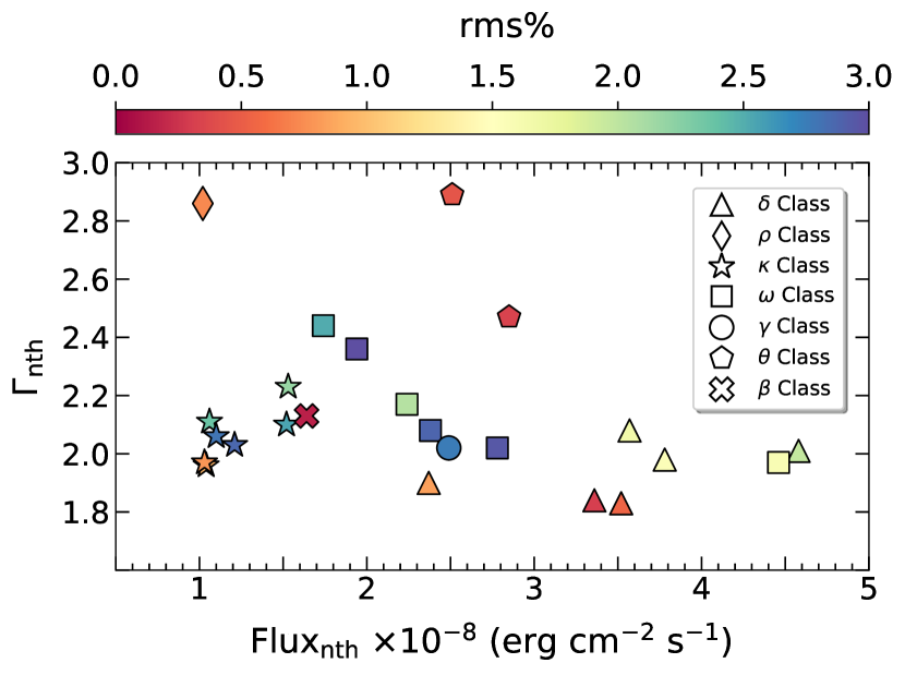
Figure 9: Variation of photon index ($\Gamma_{\rm nth}$) as a function of Comptonized flux associated with nthComp (see Table LABEL:table:Spectral_parameters) for $\delta$, $\rho$, $\kappa$, $\omega$, $\gamma$, $\theta$ and $\beta$ variability classes. The color codes denote the rms amplitudes ($rms\%$) corresponding to the detection and non-detection of HFQPOs. Obtained results for different variability classes are presented using different symbols which are marked in the inset. See text for details.

In Fig. 9, we present the variation of photon index ($\Gamma_{\rm nth}$) with the nthComp flux ($F_{\rm nth}$) for observations in $\delta$, $\rho$, $\kappa$, $\omega$, $\gamma$, $\beta$, and $\theta$ variability classes. Here, the variation of the percentage rms amplitude ($rms\%$) of the detected HFQPOs as well as the $rms\%$ of the non-detection of HFQPOs (see Table 3) are shown using color code. We find that $rms\%$ of HFQPOs lies in the range $\gtrsim$ 1.5% and it drops below $1\%$ when HFQPOs are not seen. Further, we notice that in $\omega$ class observations, $\Gamma_{\rm nth}$ decreases with the increase of nthComp flux in the range $1.8\times 10^{-8}\lesssim{\rm Flux}_{\rm nth}~{}({\rm erg~{}cm}^{-2}~{}{\rm s}^{-1})\lesssim 4.5\times 10^{-8}$. In $\kappa$ variability classes, marginal variations are observed in the nthComp flux unlike $\omega$ class observation although photon indices remain $\Gamma_{\rm nth}\gtrsim 2$ when HFQPOs are present. For $\delta$ variability classes, we find $3.5\times 10^{-8}\lesssim{\rm Flux}_{\rm nth}~{}({\rm erg~{}cm}^{-2}~{}{\rm s}^{-1})\lesssim 4.58\times 10^{-8}$ and $\Gamma_{\rm nth}\gtrsim 1.9$ for HFQPOs. In addition, we point out that HFQPOs are not seen for $\theta$, $\beta$ and $\rho$ class observations although they belong to the ‘softer’ variability classes.

6 Discussion

In this work, we carry out a comprehensive timing and spectral analyses of the BH-XRB source GRS 1915+105 using GT, AO and TOO data of entire AstroSat observations ($2016-2021$) in wide frequency ($0.01-500$ Hz) and energy ($0.7-60$ keV) bands. The variation of the hardness ratios in the CCDs and the nature of the light curves confirm the presence of seven ‘softer’ variability classes, namely $\theta$, $\beta$, $\delta$, $\rho$, $\kappa$, $\omega$, and $\gamma$ along with one additional variant of $\rho$ class ($\rho\textprime$) of the source (Athulya et al., 2021). The LAXPC count rates are found to vary in the range of $1328-10997$ cts/s, and the hardness ratios are seen to vary as $0.61\lesssim{\rm HR1}\lesssim 0.90$ and $0.02\lesssim{\rm HR2}\lesssim 0.11$. We observe similar variabilities in the low energy ($0.7-7$ keV) SXT light curves as well.

We examine the origin of the HFQPO features and find its presence only in four ‘softer’ variability classes ($\delta$, $\omega$, $\kappa$, $\gamma$). The centroid frequency and the percentage rms amplitude of the HFQPOs are found to vary in the range of $68.14-72.32$ Hz and $1.48-2.66$ per cent, respectively (see Table 2 and 3). The present findings are consistent with the earlier results reported using RXTE observations (Belloni & Altamirano, 2013a) as well as AstroSat observations (Belloni et al., 2019; Sreehari et al., 2020). It may be noted that the presence of additional peaks in the frequency range $27-41$ Hz along with HFQPOs at $67-69$ Hz was also observed (Belloni et al., 2001; Strohmayer, 2001b) in GRS 1915+105. However, we do not find any signature of additional peak in our analysis. Meanwhile, Morgan et al. (1997); Strohmayer (2001b) noticed the evolution of frequency from $\sim 67$ Hz to $\sim 69$ Hz in $\gamma$ class which is found to evolve further to $72.32^{+0.23}_{-0.21}$ Hz as seen in our observations (see Table 2 and 3). This perhaps indicates an unique characteristics of the evolution of HFQPO in a given variability class that requires further investigation.

Next, we investigate the energy dependent PDS to ascertain the photons that are responsible for the origin of the HFQPOs (see Fig. 5). We observe that HFQPO features are present in $6-25$ keV energy band in four variability classes (see Fig. 5 and Table 3). However, we do not find HFQPO signature in $\theta$, $\beta$, $\rho$ and $\chi$ variability classes (see Fig. 4 and Table 3). We find that the significance and percentage rms amplitudes of the HFQPOs are higher in $6-25$ keV energy band compared to $3-60$ keV energy band (see Table 3). Further, we study the variation of percentage rms amplitude and nthComp flux as function of energy, shown in Fig. 8. These findings are in agreement with the previous studies which were carried out considering energy bands of $2-13$ keV and $13-30$ keV only (Belloni et al., 2001). It is also found that the nthComp flux gradually decreases with energy (see Fig. 8) and beyond $\sim 25$ keV, the flux contribution becomes negligible (see Fig. 7).

We notice that $\kappa$ and $\omega$ class variabilities exhibit different duration of ‘non-dips’ (high counts $\sim 9600$ cts/s) and ‘dips’ (low counts $\sim 1250$ cts/s) features. While studying the dynamic PDS, we find that the HFQPO is generally present during ‘non-dips’ period with relatively higher rms amplitude ($2.38\pm 0.29$ and $2.35\pm 0.22$ for $\omega$ and $\kappa$ classes). We do not find the signature of HFQPO during the ‘dips’ period as seen in Fig. 6 (see also appendix A). Similar findings are also observed for $\gamma$ class variability where the HFQPO is persistently seen during the entire high count duration (see also Belloni et al., 2001).

We find that the wide-band spectra ($0.7-50$ keV) of $\theta$, $\beta$, $\delta$, $\kappa$, $\omega$ and $\gamma$ class observations are satisfactorily described by the thermal Comptonization nthComp along with a powerlaw component (see Fig. 7 and Table LABEL:table:Spectral_parameters). On the contrary, the nthComp component seems to be adequate to fit the energy spectra of $\rho$ class observations. From the spectral modelling, we obtain the range of nthComp photon index as $1.83\lesssim\Gamma_{\rm nth}\lesssim 2.89$, and electron temperature as $1.82\lesssim kT_{e}\lesssim 3.66$ keV (see Table LABEL:table:Spectral_parameters). In addition, we obtain a steep powerlaw photon index ($\Gamma_{\rm PL}$) as $2.59-3.27$ for all the variability classes under consideration. Similar steep $\Gamma_{\rm PL}$ is also reported in the previous studies carried out for $\theta$ (Belloni et al., 2006) and $\delta$ (Sreehari et al., 2020) variability classes of the source. We estimate the optical depth ($\tau$) of the surrounding medium and obtain its value as $2\lesssim\tau\lesssim 14$. This evidently indicates the presence of a cool and optically thick corona around the source, which presumably acts as a Comptonizing medium that reprocesses the soft seed photons. The Compton y-parameter is obtained in the range $0.63\pm 0.08~{}-~{}3.12\pm 0.35$ which infers that the soft photons are substantially reprocessed via Comptonization at the optically thick corona. Further, we calculate the bolometric luminosity in $0.3-100$ keV energy range for all the variability classes and find its value in the range $3-34\%$ $L_{\rm Edd}$. These findings suggest that the source possibly emits in sub-Eddington limit during the observations under consideration.

In Fig. 8, we examine the energy dependent ($6-25$ keV) $rms\%$ of HFQPOs in $\delta$, $\kappa$, $\omega$, and $\gamma$ variability classes, and find that $rms\%$ increases ($1-8\%$) with energy up to $\sim 17$ keV and then decreases. Subsequently, we observe that the Comptonize flux (${\rm Flux}_{\rm nth}$) decreases with energy which tends to become negligible beyond $25$ keV. This possibly happens when the soft photons emitted from the disc are Comptonized by the ‘hot’ electrons from an optically thick corona ($8\lesssim\tau\lesssim 12$) and produce the aforementioned Comptonized continuum. In order to elucidate the spectra above $\sim 25$ keV, an additional powerlaw component with photon index $\Gamma_{\rm PL}\sim 3$ is required. This eventually indicates that there could be an extended corona present surrounding the central corona, which is responsible for this high energy emissions (Sreehari et al., 2020). We further notice that for intermediate range of nthComp photon index ($1.97\lesssim\Gamma_{\rm nth}\lesssim 2.44$) along with the large variation of nthComp flux ($1.06\times 10^{-8}\lesssim{\rm Flux}_{\rm nth}~{}({\rm erg~{}cm}^{-2}~{}{\rm s}^{-1})\lesssim 4.46\times 10^{-8}$) generally yields HFQPO signature in $\delta$, $\kappa$, $\omega$ and $\gamma$ variability classes (see Fig. 9). With this, we argue that Comptonization process plays a viable role in exhibiting HFQPO. Overall, based on the findings presented in Fig. 8 and Fig. 9, we conjecture that HFQPOs in GRS 1915$+$105 are perhaps manifested due to the modulation of the ‘Comptonizing corona’ surrounding the central source (Méndez et al., 2013; Aktar et al., 2017, 2018; Dihingia et al., 2019; Sreehari et al., 2020).

Meanwhile, several theoretical models are put forwarded to explain the HFQPO features occasionally observed in BH-XRBs. Morgan et al. (1997) first attempted to elucidate the HFQPO features with Keplerian frequency associated with the motion of hot gas at the innermost stable circular orbit (ISCO). This model yielded high source mass as $\sim 30~{}M_{\odot}$, which is in disagreement with the dynamical mass measurement of GRS 1915+105 (Greiner et al., 2001; Reid et al., 2014) and hence dissented (Belloni & Altamirano, 2013a). Nowak et al. (1997) interpreted the origin of $67$ Hz QPO in GRS 1915+105 as the resulting frequency of the lowest radial g-mode oscillation in the accretion disc. However, this model lacks cogency for those BH-XRBs that generally manifest $>10\%$ rms amplitude variability. Further, there were alternative attempts to address the origin of HFQPO without dwelling much on observational features (Chen & Taam, 1995; Rezzolla et al., 2003; Stuchlík et al., 2007). Noticing significant hard lag in GRS 1915+105, Cui (1999) infer that a Comptonizing region is responsible for the HFQPOs. Remillard et al. (2002) further stressed on the presence of ‘Compton corona’ that reprocesses the disk photons and yields HFQPO features. In addition, Aktar et al. (2017, 2018) reported that the HFQPO features of GRO J1655$-$40 at $300$ Hz and $450$ Hz perhaps resulted due to the modulations of the post-shock corona (PSC) that radiates Comptonized emissions (Chakrabarti & Titarchuk, 1995). Recently, Dihingia et al. (2019) ascertained that the shock induced relativistic accretion solutions are potentially viable to explain the HFQPOs in well studied BH-XRB sources, namely GRS 1915$+$105 and GRO J1655$-$40. With this, we affirm that the HFQPO models proposed based on the ‘Comptonizing corona’ fervently favor our observational findings delineated in this work.

7 Conclusions

In this paper, we perform in-depth temporal and spectral analyses in the wide-band ($0.7-60$ keV) energy range of the BH-XRB source GRS 1915+105 using entire AstroSat observations ($2016-2021$) in seven ‘softer’ variability classes, namely $\theta$, $\beta$, $\delta$, $\rho$, $\kappa$, $\omega$ and $\gamma$, and one ‘harder’ variability class ($\chi$), respectively. The overall findings of this work are summarized below:

• We find HFQPO feature in $\delta$, $\kappa$, $\omega$ and $\gamma$ classes of GRS 1915 + 105 having frequency in the range $68.14-72.32$ Hz. However, we did not find the signature of HFQPO features in $\theta$, $\beta$, $\rho$, and $\chi$ class observations.

• Energy dependent PDS study indicates that the emergent photons in the energy range $6-25$ keV seem to be responsible for generating the HFQPO features. Beyond this energy range, the HFQPO signature is not detected. We notice that percentage rms amplitude ($rms\%$) of HFQPOs increases ($1-8\%$) with energy up to $\sim 17$ keV and then decreases.

• Dynamical PDS of $\kappa$ and $\omega$ classes reveal that the ‘non-dips’ (high count) features of the light curve are possibly linked with the generation of HFQPOs.

• The wide-band spectral modelling indicates that in presence of HFQPO, the thermal Comptonization components ($1.06\times 10^{-8}\lesssim F_{\rm nth}~{}({\rm erg}{\rm~{}cm}^{-2}{\rm~{}s}^{-1})\lesssim 4.46\times 10^{-8}$) having $\Gamma_{\rm nth}$ of $1.97-2.44$ dominate (up to $\sim 25$ keV) over the additional powerlaw component ($0.52\times 10^{-8}\lesssim F_{\rm PL}~{}({\rm erg}{\rm~{}cm}^{-2}{\rm~{}s}^{-1})\lesssim 1.37\times 10^{-8}$) with $\Gamma_{PL}$ $\sim 3$ (above $\sim 25$ keV).

With the above findings, we argue that the variability produced during the ‘softer’ classes of GRS 1915+105 is possibly due to the modulation of the Comptonizing corona that manifests the HFQPO features.

Data Availability

Data used for this publication are currently available at the Astrobrowse (AstroSat archive) website (https://astrobrowse.issdc.gov.in/astro_archive/archive) of the Indian Space Science Data Center (ISSDC).

Appendix A Intensity dependent power spectra

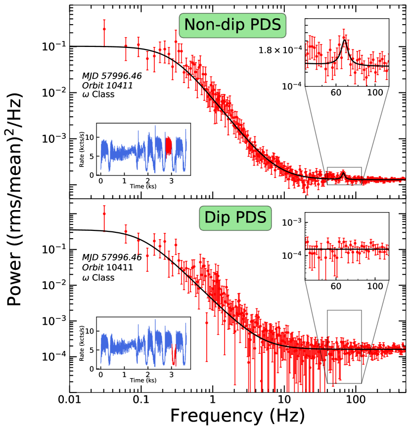
Figure 10: Top: Power density spectrum (PDS) corresponding to one ‘non-dip’ (high counts) duration (red segment of the light curve) of $\omega$ class observation (Orbit 10411) in a wide frequency range of $0.01-500$ Hz. Bottom: PDS corresponding to one ‘dip’ (low counts) duration (red segment of the light curve). Both PDS are obtained for the energy band of $3-60$ keV with LAXPC10 and LAXPC20 combined observations. In each panel, zoomed view of the high frequency region of the PDS is depicted at the inset.

The power spectra are generated separately considering both ‘non-dips’ (high counts) and ‘dips’ (low counts) duration of the light curve (Orbit 10411, $\omega$ class). In the top panel of Figure A1, we show the power spectrum corresponding to the ‘non-dip’ segment of the light curve shown at the bottom-left inset using red color. The HFQPO signature around $67.08^{+1.05}_{-1.35}$ Hz is distinctly visible ($rms\%=2.38\pm 0.29$) at the top-right inset. In the lower panel, we plot the power spectrum obtained for the ‘dip’ segment of the light curve which is indicated in red color at the bottom-left inset. The HFQPO feature is not seen ($rms\%=0.67\pm 0.18$) as shown at the top-right inset. We further confirm that similar findings are observed during $\kappa$ class observation (Orbit 9895) as well, where $rms\%$ of the HFQPO feature for ‘non-dips’ and ‘dips’ duration are obtained as $2.35\pm 0.22$ and $0.26\pm 0.10$, respectively.

References

- Abramowicz & Kluźniak (2001) Abramowicz M. A., Kluźniak W., 2001, A&A, 374, L19
- Agrawal (2006) Agrawal P. C., 2006, Advances in Space Research, 38, 2989
- Agrawal et al. (2017) Agrawal P. C., et al., 2017, Journal of Astrophysics and Astronomy, 38, 30
- Agrawal et al. (2018) Agrawal V. K., Nandi A., Girish V., Ramadevi M. C., 2018, MNRAS, 477, 5437
- Aktar et al. (2017) Aktar R., Das S., Nandi A., Sreehari H., 2017, MNRAS, 471, 4806
- Aktar et al. (2018) Aktar R., Das S., Nandi A., Sreehari H., 2018, Journal of Astrophysics and Astronomy, 39, 17
- Altamirano & Belloni (2012) Altamirano D., Belloni T., 2012, ApJ, 747, L4
- Antia et al. (2017) Antia H. M., et al., 2017, ApJS, 231, 10
- Antia et al. (2021) Antia H. M., et al., 2021, Journal of Astrophysics and Astronomy, 42, 32
- Athulya et al. (2021) Athulya M. P., Radhika D., Agrawal V. K., Ravishankar B. T., Naik S., Mandal S., Nandi A., 2021, MNRAS, Under Review
- Baby et al. (2020) Baby B. E., Agrawal V. K., Ramadevi M. C., Katoch T., Antia H. M., Mandal S., Nandi A., 2020, MNRAS, 497, 1197
- Banerjee et al. (2021) Banerjee A., Bhattacharjee A., Chatterjee D., Debnath D., Chakrabarti S. K., Katoch T., Antia H. M., 2021, ApJ, 916, 68
- Belloni & Altamirano (2013a) Belloni T. M., Altamirano D., 2013a, MNRAS, 432, 10
- Belloni & Altamirano (2013b) Belloni T. M., Altamirano D., 2013b, MNRAS, 432, 19
- Belloni & Stella (2014) Belloni T. M., Stella L., 2014, Space Sci. Rev., 183, 43
- Belloni et al. (2000) Belloni T., Klein-Wolt M., Méndez M., van der Klis M., van Paradijs J., 2000, A&A, 355, 271
- Belloni et al. (2001) Belloni T., Méndez M., Sánchez-Fernández C., 2001, A&A, 372, 551
- Belloni et al. (2006) Belloni T., Soleri P., Casella P., Méndez M., Migliari S., 2006, MNRAS, 369, 305
- Belloni et al. (2012) Belloni T. M., Sanna A., Méndez M., 2012, MNRAS, 426, 1701
- Belloni et al. (2019) Belloni T. M., Bhattacharya D., Caccese P., Bhalerao V., Vadawale S., Yadav J. S., 2019, MNRAS, 489, 1037
- Beloborodov (1999) Beloborodov A. M., 1999, ApJ, 510, L123
- Castro-Tirado et al. (1992) Castro-Tirado A. J., Brandt S., Lund N., 1992, IAU, 5590
- Chakrabarti & Titarchuk (1995) Chakrabarti S., Titarchuk L. G., 1995, ApJ, 455, 623
- Chatterjee et al. (2021) Chatterjee R., Agrawal V. K., Nandi A., 2021, arXiv e-prints, p. arXiv:2105.09051
- Chen & Taam (1995) Chen X., Taam R. E., 1995, ApJ, 441, 354
- Cui (1999) Cui W., 1999, ApJ, 524, L59
- Cui (2000) Cui W., 2000, ApJ, 534, L31
- Dihingia et al. (2019) Dihingia I. K., Das S., Maity D., Nandi A., 2019, MNRAS, 488, 2412
- Fender et al. (1999) Fender R., et al., 1999, ApJ, 519, L165
- Frank et al. (2002) Frank J., King A., Raine D. J., 2002, Accretion Power in Astrophysics: Third Edition
- Greiner et al. (2001) Greiner J., Cuby J. G., McCaughrean M. J., 2001, Nature, 414, 522
- Haardt et al. (1993) Haardt F., Done C., Matt G., Fabian A. C., 1993, ApJ, 411, L95
- Hannikainen et al. (2005) Hannikainen D. C., et al., 2005, A&A, 435, 995
- Homan et al. (2001) Homan J., Wijnands R., van der Klis M., Belloni T., van Paradijs J., Klein-Wolt M., Fender R., Méndez M., 2001, ApJS, 132, 377
- Homan et al. (2003) Homan J., Klein-Wolt M., Rossi S., Miller J. M., Wijnands R., Belloni T., van der Klis M., Lewin W. H. G., 2003, ApJ, 586, 1262
- Homan et al. (2005) Homan J., Miller J. M., Wijnands R., van der Klis M., Belloni T., Steeghs D., Lewin W. H. G., 2005, ApJ, 623, 383
- Huppenkothen et al. (2019) Huppenkothen D., et al., 2019, ApJ, 881, 39
- Iyer et al. (2015) Iyer N., Nandi A., Mandal S., 2015, ApJ, 807, 108
- Katoch et al. (2021) Katoch T., Baby B. E., Nandi A., Agrawal V. K., Antia H. M., Mukerjee K., 2021, MNRAS, 501, 6123
- Klein-Wolt et al. (2002) Klein-Wolt M., Fender R. P., Pooley G. G., Belloni T., Migliari S., Morgan E. H., van der Klis M., 2002, MNRAS, 331, 745
- Klein-Wolt et al. (2004) Klein-Wolt M., Homan J., van der Klis M., 2004, Nuclear Physics B Proceedings Supplements, 132, 381
- Leahy & Chen (2019) Leahy D. A., Chen Y., 2019, ApJ, 871, 152
- Leahy et al. (1983) Leahy D. A., Darbro W., Elsner R. F., Weisskopf M. C., Sutherland P. G., Kahn S., Grindlay J. E., 1983, ApJ, 266, 160
- Lucchini et al. (2021) Lucchini M., et al., 2021, arXiv e-prints, p. arXiv:2108.12011
- Mandal & Chakrabarti (2005) Mandal S., Chakrabarti S. K., 2005, A&A, 434, 839
- Markoff et al. (2005) Markoff S., Nowak M. A., Wilms J., 2005, ApJ, 635, 1203
- McClintock & Remillard (2006) McClintock J. E., Remillard R. A., 2006, Black hole binaries. pp 157–213
- Méndez et al. (2013) Méndez M., Altamirano D., Belloni T., Sanna A., 2013, MNRAS, 435, 2132
- Miller et al. (2001) Miller J. M., et al., 2001, ApJ, 563, 928
- Mirabel & Rodríguez (1994) Mirabel I. F., Rodríguez L. F., 1994, Nature, 371, 46
- Morgan et al. (1997) Morgan E. H., Remillard R. A., Greiner J., 1997, ApJ, 482, 993
- Nandi et al. (2001) Nandi A., Manickam S. G., Rao A. R., Chakrabarti S. K., 2001, MNRAS, 324, 267
- Nowak et al. (1997) Nowak M. A., Wagoner R. V., Begelman M. C., Lehr D. E., 1997, ApJ, 477, L91
- Nowak et al. (2011) Nowak M. A., et al., 2011, ApJ, 728, 13
- Poutanen et al. (2018) Poutanen J., Veledina A., Zdziarski A. A., 2018, A&A, 614, A79
- Ratti et al. (2012) Ratti E. M., Belloni T. M., Motta S. E., 2012, Monthly Notices of the Royal Astronomical Society, 423, 694
- Reid et al. (2014) Reid M. J., McClintock J. E., Steiner J. F., Steeghs D., Remillard R. A., Dhawan V., Narayan R., 2014, ApJ, 796, 2
- Remillard & McClintock (2006) Remillard R. A., McClintock J. E., 2006, ARA&A, 44, 49
- Remillard et al. (1999) Remillard R. A., Morgan E. H., McClintock J. E., Bailyn C. D., Orosz J. A., 1999, ApJ, 522, 397
- Remillard et al. (2002) Remillard R. A., Muno M. P., McClintock J. E., Orosz J. A., 2002, ApJ, 580, 1030
- Remillard et al. (2006) Remillard R. A., McClintock J. E., Orosz J. A., Levine A. M., 2006, ApJ, 637, 1002
- Rezzolla et al. (2003) Rezzolla L., Yoshida S., Maccarone T. J., Zanotti O., 2003, MNRAS, 344, L37
- Ribeiro et al. (2019) Ribeiro E. M., Méndez M., de Avellar M. G. B., Zhang G., Karpouzas K., 2019, MNRAS, 489, 4980
- Shakura & Sunyaev (1973) Shakura N. I., Sunyaev R. A., 1973, A&A, 24, 337
- Singh et al. (2017) Singh K. P., et al., 2017, Journal of Astrophysics and Astronomy, 38, 29
- Sreehari et al. (2019) Sreehari H., Ravishankar B. T., Iyer N., Agrawal V. K., Katoch T. B., Mandal S., Nand i A., 2019, MNRAS, 487, 928
- Sreehari et al. (2020) Sreehari H., Nandi A., Das S., Agrawal V. K., Mandal S., Ramadevi M. C., Katoch T., 2020, MNRAS, 499, 5891
- Strohmayer (2001a) Strohmayer T. E., 2001a, ApJ, 552, L49
- Strohmayer (2001b) Strohmayer T. E., 2001b, ApJ, 554, L169
- Stuchlík et al. (2007) Stuchlík Z., Slaný P., Török G., 2007, A&A, 470, 401
- Sunyaev & Titarchuk (1980) Sunyaev R. A., Titarchuk L. G., 1980, A&A, 86, 121
- Tanaka & Lewin (1995) Tanaka Y., Lewin W. H. G., 1995, X-ray Binaries, pp 126–174
- Vadawale et al. (2001) Vadawale S. V., Rao A. R., Chakrabarti S. K., 2001, A&A, 372, 793
- Vadawale et al. (2016) Vadawale S. V., et al., 2016, in den Herder J.-W. A., Takahashi T., Bautz M., eds, Society of Photo-Optical Instrumentation Engineers (SPIE) Conference Series Vol. 9905, Space Telescopes and Instrumentation 2016: Ultraviolet to Gamma Ray. p. 99051G (arXiv:1609.00538), doi:10.1117/12.2235373
- Wang et al. (2021) Wang J., et al., 2021, ApJ, 910, L3
- Wilms et al. (2000) Wilms J., Allen A., McCray R., 2000, ApJ, 542, 914
- Yadav et al. (2016) Yadav J. S., et al., 2016, in den Herder J.-W. A., Takahashi T., Bautz M., eds, Society of Photo-Optical Instrumentation Engineers (SPIE) Conference Series Vol. 9905, Space Telescopes and Instrumentation 2016: Ultraviolet to Gamma Ray. p. 99051D, doi:10.1117/12.2231857
- Zdziarski et al. (1996) Zdziarski A. A., Johnson W. N., Magdziarz P., 1996, MNRAS, 283, 193
- van der Klis (1988) van der Klis M., 1988, in Ögelman H., van den Heuvel E. P. J., eds, NATO Advanced Science Institutes (ASI) Series C Vol. 262, NATO Advanced Science Institutes (ASI) Series C. Kluwer Academic Publishers, Dordrecht, p. 27