Learning Affinity from Attention: End-to-End Weakly-Supervised Semantic Segmentation with Transformers

Abstract

Weakly-supervised semantic segmentation (WSSS) with image-level labels is an important and challenging task. Due to the high training efficiency, end-to-end solutions for WSSS have received increasing attention from the community. However, current methods are mainly based on convolutional neural networks and fail to explore the global information properly, thus usually resulting in incomplete object regions. In this paper, to address the aforementioned problem, we introduce Transformers, which naturally integrate global information, to generate more integral initial pseudo labels for end-to-end WSSS. Motivated by the inherent consistency between the self-attention in Transformers and the semantic affinity, we propose an Affinity from Attention (AFA) module to learn semantic affinity from the multi-head self-attention (MHSA) in Transformers. The learned affinity is then leveraged to refine the initial pseudo labels for segmentation. In addition, to efficiently derive reliable affinity labels for supervising AFA and ensure the local consistency of pseudo labels, we devise a Pixel-Adaptive Refinement module that incorporates low-level image appearance information to refine the pseudo labels. We perform extensive experiments and our method achieves 66.0% and 38.9% mIoU on the PASCAL VOC 2012 and MS COCO 2014 datasets, respectively, significantly outperforming recent end-to-end methods and several multi-stage competitors. Code is available at https://github.com/rulixiang/afa.

1 Introduction

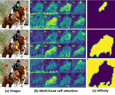
Figure 1: (a) Image and the query points (denote with ”$\bigstar$”) to visualize the attention and affinity maps; (b) the self-attention maps in Transformer blocks only capture coarse semantic-level affinity relations; (c) the learned reliable semantic affinity from self-attention with our proposed method.

Semantic segmentation, aiming at labeling each pixel in an image, is a fundamental task in vision. In the past decade, deep neural networks have achieved great success in semantic segmentation. However, due to the data-hungry nature of deep neural networks, fully-supervised semantic segmentation models usually require a large amount of data with labour intensive pixel-level annotations. To settle this problem, some recent methods seek to devise semantic segmentation models using weak/cheap labels, such as image-level labels [2, 25, 47, 23, 50, 27, 35], points [3], scribbles [28, 54, 52], and bounding boxes [24]. Our method falls into the category of weakly-supervised semantic segmentation (WSSS) using only image-level labels, which is the most challenging one in all WSSS scenarios.

Prevailing WSSS methods with image-level labels commonly adopt a multi-stage framework [35, 23, 22]. Specifically, these methods firstly train a classification model and then generate Class Activation Maps (CAM) [59] as the pseudo labels. After refinement, the pseudo labels are leveraged to train a standalone semantic segmentation network as the final model. This multi-stage framework needs to train multiple models for different purposes, thus obviously complicating the training streamline and slowing down the efficiency. To avoid this problem, several end-to-end solutions have been recently proposed for WSSS [4, 52, 53, 3]. However, these methods are commonly based on convolution neural networks and fail to explore the global feature relations properly, which turns out to be crucial for activating integral object regions [13], thus significantly affecting the quality of generated pseudo labels.

Recently, Transformers [42] have achieved significant breakthroughs in numerous visual applications [49, 58, 5]. We argue that the Transformer architecture naturally benefits the WSSS task. Firstly, the self-attention mechanism in Transformers could model the global feature relations and conquer the aforementioned drawback of convolutional neural networks, thus discovering more integral object regions. As shown in Fig. 1, we find that the multi-head self-attention (MHSA) in Transformers could capture semantic-level affinity, and can thus be used to improve the coarse pseudo labels. However, the affinity captured in MHSA is still inaccurate (Fig. 1(b)), , directly applying MHSA as affinity to revise the labels does not work well in practice, which is shown in Fig. 2 (c).

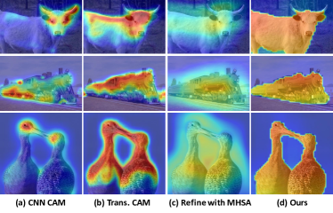
Figure 2: CAM generated with (b) Transformers activates more integral regions than (a) CNN. Refining CAM with (c) coarse MHSA doesn’t work well, while (d) the learned affinity could remarkably improve the generated CAM.

Based on the above analysis, we propose a Transformer-based end-to-end framework for WSSS. Specifically, we leverage Transformers to generate CAM as the initial pseudo labels, to avoid the intrinsic drawback of convolutional neural networks. We further exploit the inherent affinity in Transformer blocks to improve the initial pseudo labels. Since the semantic affinity in MHSA is coarse, we propose an Affinity from Attention (AFA) module, which aims to derive reliable pseudo affinity labels to supervise the semantic affinity learned from the MHSA in Transformer. The learned affinity is then employed to revise the initial pseudo labels via random walk propagation [2, 1], which could diffuse object regions and dampen the falsely activated regions. To derive highly-confident pseudo affinity labels for AFA and ensure the local consistency of the propagated pseudo labels, we further propose a Pixel-Adaptive Refinement module (PAR). Based on the pixel-adaptive convolution [4, 37], PAR efficiently integrates the RGB and position information of local pixels to refine the pseudo labels, enforcing better alignment with low-level image appearance. In addition, given the simplicity, our model can be trained in an end-to-end manner, thus avoiding a complex training pipeline. Experimental results on PASCAL VOC 2012 [12] and MS COCO 2014 [29] demonstrate that our method remarkably surpasses recent end-to-end methods and several multi-stage competitors.

In summary, our contributions are listed as follows.

• We propose an end-to-end Transformer-based framework for WSSS with image-level labels. To the best of our knowledge, this is the first work to explore Transformers for WSSS.

• We exploit the inherent virtue of Transformer and devise an Affinity from Attention (AFA) module. AFA learns reliable semantic affinity from MHSA and propagates the pseudo labels with the learned affinity.

• We propose an efficient Pixel-Adaptive Refinement (PAR) module, which incorporates the RGB and position information of local pixels for label refinement.

2 Related Work

2.1 Weakly-Supervised Semantic Segmentation

Multi-stage Methods. Most WSSS methods with image-level labels are accomplished in a multi-stage process. Commonly, these approaches train a classification network to produce the initial pseudo pixel-level labels with CAM. To address the drawback of incomplete object activation of CAM, [46, 56, 40] utilize Erasing strategy to erase the most discriminative regions and thus discover more complete object regions. Inspired by the observation that the classification network tends to focus on different object regions at different training stages, [16, 51, 18] accumulate the activated regions in the training process. [26, 39, 47] propose to mine semantic regions from multiple input images, discovering similar semantic regions. A prevailing group of WSSS trains classification network with auxiliary tasks to ensure integral object discovery [45, 7, 35, 36]. Some recent researches interpret CAM generation from novel perspectives, such as causal inference [55], information bottleneck theory [22], and anti-adversarial attack [23].

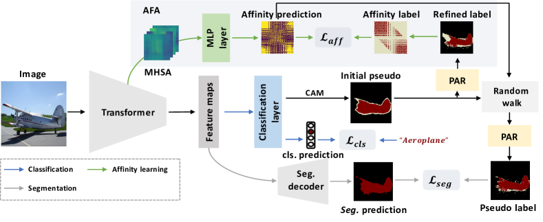
Figure 3: The proposed end-to-end framework for WSSS. We use a Transformer backbone as the encoder to extract feature maps. The initial pseudo labels are generated with CAM [59] and then refined with the proposed PAR. In the AFA module, we derive the semantic affinity from MHSA in Transformer blocks. AFA is supervised with the pseudo affinity labels derived from the refined label. Next, we employ the learned affinity to revise the pseudo labels via random walk propagation [2, 1]. The propagated labels are finally refined with PAR as the pseudo labels for the segmentation branch.

End-to-End Methods. Due to the extremely limited supervision, training an end-to-end model for WSSS with favorable performance is difficult. [31] proposes an adaptive Expectation-Maximization framework to infer pseudo ground truth for segmentation. [32] tackles WSSS with image-level labels as a multi-instance learning (MIL) problem and devises the Log-Sum-Exp aggregation function to drive the network to assign correct pixel labels. Incorporating nGWP pooling, pixel-adaptive mask refinement, and stochastic low-level information transfer, 1Stage [4] achieves comparable performance with multi-stage models. In [53], RRM takes CAM as the initial pseudo labels and employs CRF [20] to produce the refined label as supervision for segmentation. RRM also introduces an auxiliary regularization loss [41] to ensure the consistency between segmentation map and low-level image appearance. [57] introduces the adaptive affinity field [17] with weighted affinity kernels and feature-to-prototype alignment loss to ensure the semantic fidelity. The above methods commonly adopt CNN and raise the inherent drawback of convolution, , failing to capture the global information, leading to the incomplete activation of objects [13]. In this work, we explore Transformers for end-to-end WSSS to address this issue.

2.2 Transformer in Vision

In [11], Dosovitskiy et al.proposes Vision Transformer (ViT), the first work to apply pure Transformer architecture for visual recognition tasks, achieving astonishing performance on visual classification benchmarks. Later variants show ViT also benefits downstream vision tasks, such as semantic segmentation [49, 9, 58], depth estimation [33], and video understanding [5]. In [13], Gao et al.proposes the first Transformers-based method (TS-CAM) for weakly-supervised object localization (WSOL). Close to WSSS, WSOL aims at localizing objects with only image-level supervision. TS-CAM trains a ViT model with image-level supervision, generates semantic-aware CAM, and couples the generated CAM with semantic-agnostic attention maps. The semantic-agnostic attention maps are derived from the attention of class token against other patch tokens. Nevertheless, TS-CAM didn’t exploit the intrinsic semantic affinity in MHSA to promote the localization results. In this work, we propose to learn the reliable semantic affinity from MHSA and propagate CAM with the learned affinity.

3 Methodology

In this section, we first introduce the Transformer backbone and CAM to generate initial pseudo labels. We then present the Affinity from Attention (AFA) module to learn reliable semantic affinity and propagate the initial pseudo labels with the learned affinity. Afterward, we introduce a Pixel-Adaptive Refinement (PAR) module to ensure the local consistency of pseudo labels. The overall loss function for optimization is presented in Section 3.5.

3.1 Transformer Backbone

As shown in Fig. 3, our framework uses the Transformers as the backbone. An input image is firstly split into $h\times w$ patches, where each patch is flattened and linearly projected to form $h\times w$ tokens. In each Transformer block, the multi-head self-attention (MHSA) is used to capture global feature dependencies. Specifically, for the $i^{th}$ head, patch tokens are projected with Multi-Layer Perception (MLP) layers and construct queries $Q_{i}\in\mathbb{R}^{hw\times d_{k}}$, keys $K_{i}\in\mathbb{R}^{hw\times d_{k}}$, and values $V_{i}\in\mathbb{R}^{hw\times d_{v}}$. $d_{k}$ is feature dimension of queries and keys, and $d_{v}$ denotes the feature dimension of values. Based on $Q_{i}$, $K_{i}$ and $V_{i}$, the self-attention matrix ${S_{i}}$ and outputs $X_{i}$ are

$$S_{i}=\frac{{Q_{i}}{K_{i}}^{\top}}{\sqrt{d_{k}}},\quad X_{i}=\mathtt{softmax}({S_{i}})V_{i}.$$ (1)

The final output $X_{o}$ of the Transformer block is constructed by feeding $(X_{1}\|X_{2}\|...\|X_{n})$ into feed-forward layers (FFN), , $X_{o}=\mathtt{FFN}(X_{1}\|X_{2}\|...\|X_{n})$, where $\mathtt{FFN}(\cdot)$ consists of Layer Normalization [6] and MLP layers. $(\cdot\|\cdot)$ denotes the concatenation operation. By stacking multiple Transformer blocks, the backbone produces feature maps for the subsequent modules.

3.2 CAM Generation

Considering the simplicity and inference efficiency, we adopt class activation maps (CAM) [59] as the initial pseudo labels. For the extracted feature maps $F\in\mathbb{R}^{hw\times d}$ and a given class $c$, the activation map $M^{c}$ is generated via weighting the feature maps in $F$ with their contribution to class $c$, , the weight matrix $W$ in the classification layer,

$$\small\begin{split}{M}^{c}&=\mathtt{ReLu}\Bigl{(}\sum_{i=1}^{d}{W}^{i,c}{F}^{i}\Bigr{)},\end{split}$$ (2)

where ReLu function is used to remove the negative activations. Min-Max normalization is applied to scale $M^{c}$ to $[0,1]$. A background score $\beta$ ($0<\beta<1$) is then used to differentiate foreground and background regions.

3.3 Affinity from Attention

As shown in Fig. 1, we notice the consistency between MHSA in Transformers and the semantic-level affinity, which motivates us to use MHSA to discover the object regions. However, since no explicit constraints are imposed on self-attention matrices during the training process, the learned affinity in MHSA is typically coarse and inaccurate, which means directly applying MHSA as affinity to refine the initial labels does not work well (Fig 2 (c)). Therefore, we propose the Affinity from Attention module (AFA) to counter this problem.

Assuming MHSA in a Transformer block is denoted as $S\in\mathbb{R}^{hw\times hw\times n}$, where $hw$ is the flattened spatial size and $n$ is the number of attention heads. In our AFA module, we directly produce the semantic affinity by linearly combining the multi-head attention, , using an MLP layer. Essentially, the self-attention mechanism is a kind of directed graphical model [43], while the affinity matrix should be symmetric since nodes sharing the same semantics are supposed to be equal. To perform such transformation, we simply add $S$ and its transpose. The predicted semantic affinity matrix $A\in\mathbb{R}^{hw\times hw}$ is thus denoted as

$$A=\mathtt{MLP}(S+S^{\top}).$$ (3)

Here, we use the matrix transpose operator ^⊤ to denote the transpose of each self-attention matrix in tensor $S$.

Pseudo Affinity Label Generation. To learn the favorable semantic affinity ${A}$, a key step is to derive a reliable pseudo affinity label $Y_{aff}$ as supervision. As shown in Fig. 3, we derive $Y_{aff}$ from the refined pseudo labels (the refinement module will be introduced later).

We first use two background scores $\beta_{l}$ and $\beta_{h}$, where $0<\beta_{l}<\beta_{h}<1$, to filter the refined pseudo labels to reliable foreground, background, and uncertain regions. Formally, given CAM $M\in\mathbb{R}^{h\times w\times C}$, the pseudo label $Y_{p}$ is constructed as

$$Y_{p}^{i,j}=\left\{\begin{aligned} &\mathtt{argmax}(M^{i,j,:}),&\text{if $\mathtt{max}(M^{i,j,:})\geq\beta_{h}$,}\\ &0,&\text{if $\mathtt{max}(M^{i,j,:})\leq\beta_{l}$,}\\ &255,&\text{otherwise,}\\ \end{aligned}\right.$$ (4)

where $0$ and $255$ denote the index of the background class and the ignored regions, respectively. $\mathtt{argmax}(\cdot)$ extracts the semantic class with the maximum activation value.

The pseudo affinity label $Y_{aff}\in\mathbb{R}^{hw\times hw}$ is then derived from $Y_{p}$. Specifically, for $Y_{p}$, if the pixel $(i,j)$ and $(k,l)$ share the same semantic, we set their affinity as positive; otherwise, their affinity is set as negative. Note that if pixels $(i,j)$ or $(k,l)$ are sampled from the ignored regions, their affinity will also be ignored. Besides, we only consider the situation that pixel $(i,j)$ and $(k,l)$ are in the same local window, and disregard the affinity of distant pixel pairs.

Affinity Loss. The generated pseudo affinity label $Y_{aff}$ is then used to supervise the predicted affinity $A$. The affinity loss term $\mathcal{L}_{aff}$ is constructed as

$$\mathcal{L}_{aff} =\frac{1}{N^{+}}\sum_{(ij,kl)\in\mathcal{R}^{+}}(1-\mathtt{sigmoid}(A^{ij,kl}))$$ (5)

$$+\frac{1}{N^{-}}\sum_{(ij,kl)\in\mathcal{R}^{-}}\mathtt{sigmoid}(A^{ij,kl}),$$

where $\mathcal{R}^{+}$ and $\mathcal{R}^{-}$ denote the set of positive and negative samples in $Y_{aff}$, respectively. $N^{+}$ and $N^{-}$ count the number of $\mathcal{R}^{+}$ and $\mathcal{R}^{-}$. Intuitively, Eq. 5 enforces the network to learn highly confident semantic affinity relations from MHSA. On the other hand, since the affinity prediction $A$ is the linear combination of MHSA, Eq. 5 also benefits the learning of self-attention and further helps to discover the integral object regions.

Propagation with Affinity. The learned reliable semantic affinity could be used to revise the initial CAM. Following [2, 1], we fulfill this process via random walk [44]. For the learned semantic affinity matrix $A$, the semantic transition matrix $T$ is derived as

$$T=D^{-1}A^{\alpha},\quad\text{with $D^{ii}=\sum_{k}{A^{ik}}^{\alpha}$,}$$ (6)

where $\alpha>1$ is a hyper-parameter to ignore trivial affinity values in $A$, and $D$ is a diagonal matrix to normalize $A$ row-wise. The random walk propagation for the initial CAM $M\in\mathbb{R}^{h\times w\times C}$ is accomplished as

$$M_{aff}=T*\mathtt{vec}(M),$$ (7)

where $\mathtt{vec}(\cdot)$ vectorizes $M$. This propagation process diffuses the semantic regions with high affinity and dampens the wrongly activated regions so that the activation maps align better with semantic boundaries.

3.4 Pixel-Adaptive Refinement

As shown in Fig. 3, the pseudo affinity label $Y_{aff}$ is derived from the initial pseudo labels. However, the initial pseudo labels are typically coarse and locally inconsistent, , neighbor pixels with similar low-level image appearance may not share the same semantic. To ensure the local consistency, [19, 53, 57] adopt dense CRF [20] to refine the initial pseudo labels. However, CRF is not a favorable choice in end-to-end framework since it remarkably slows down the training efficiency. Inspired by [4], which utilizes the pixel-adaptive convolution [37] to extract local RGB information for refinement, we incorporate the RGB and spatial information to define the low-level pairwise affinity and construct our Pixel-Adaptive Refinement module (PAR).

Given the input image $I\in\mathbb{R}^{h\times w\times 3}$, for the pixel at position $(i,j)$ and $(k,l)$, the RGB and spatial pairwise terms are defined as:

$$\small\kappa^{ij,kl}_{rgb}=-\Bigl{(}\frac{|I_{ij}-I_{kl}|}{w_{1}{\sigma^{ij}_{rgb}}}\Bigr{)}^{2},\quad\kappa^{ij,kl}_{pos}=-\Bigl{(}\frac{|P_{ij}-P_{kl}|}{w_{2}{\sigma^{ij}_{pos}}}\Bigr{)}^{2},$$ (8)

where $I_{ij}$ and $P_{ij}$ denote the RGB information and the spatial location of pixel $(i,j)$, respectively. In practice, we use the XY coordinates as the spatial location. In Eq. 8, $\sigma_{rgb}$ and $\sigma_{pos}$ denote the standard deviation of RGB and position difference, respectively. $w_{1}$ and $w_{2}$ control the smoothness of $\kappa_{rgb}$ and $\kappa_{pos}$, respectively. The affinity kernel for PAR is then constructed by normalizing $\kappa_{rgb}$ and $\kappa_{pos}$ with softmax and adding them together, ,

$$\small\kappa^{ij,kl}=\frac{\exp(\kappa^{ij,kl}_{rgb})}{\sum_{(x,y)}\exp(\kappa^{ij,xy}_{rgb})}+w_{3}\frac{\exp(\kappa^{ij,kl}_{pos})}{\sum_{(x,y)}\exp(\kappa^{ij,xy}_{pos})},$$ (9)

where $(x,y)$ is sampled from the neighbor set of $(i,j)$, $\mathcal{N}(i,j)$, and $w_{3}$ adjusts the importance of the position term. Based on the constructed affinity kernel, we refine both the initial CAM and the propagated CAM. The refinement is conducted for multiple iterations. For CAM ${M}\in\mathbb{R}^{h\times w\times C}$, in iteration $t$, we have

$${M}^{i,j,c}_{t}=\sum_{(k,l)\in\mathcal{N}(i,j)}\kappa^{ij,kl}{M}^{k,l,c}_{t-1}.$$ (10)

For the neighbor pixel sets $\mathcal{N}(\cdot)$, we follow [4] and define it as the 8-way neighbors with multiple dilation rates. Such design ensures the training efficiency, since the dilated neighbors of a given pixel can be easily extracted using $3\times 3$ dilated convolutions.

3.5 Network Training

As shown in Fig. 3, our framework consists of three loss terms, , a classification loss $\mathcal{L}_{cls}$, a segmentation loss $\mathcal{L}_{seg}$, and an affinity loss $\mathcal{L}_{aff}$.

For the classification loss, following the common practice, we feed the aggregated features into a classification layer to compute the class probability vector $p_{cls}$, then employ the multi-label soft margin loss as the classification function.

$$\mathcal{L}_{cls}=\frac{1}{C}\sum_{c=1}^{C}(y^{c}\log(p_{cls}^{c})+(1-{y}^{c})\log(1-{p}_{cls}^{c})),$$ (11)

where $C$ is the total number of classes, and $y$ is the ground truth image-level label.

For the segmentation loss $\mathcal{L}_{seg}$, we adopt the commonly-used cross-entropy loss. As shown in Fig. 3, the supervision for the segmentation branch is the revised label with affinity propagation. In order to obtain better alignment with low-level image appearance, we use the proposed PAR to further refine the propagated labels. The affinity loss $\mathcal{L}_{aff}$ for affinity learning is previously described in Eq. 5.

The overall loss is the weighted sum of $\mathcal{L}_{cls}$, $\mathcal{L}_{aff}$, and $\mathcal{L}_{seg}$. In addition, to further promote the performance, we also employ the regularization loss $\mathcal{L}_{reg}$ used in [41, 57, 54, 53], which ensures the local consistency of the segmentation predictions. The overall loss is finally formulated as

$$\mathcal{L}=\mathcal{L}_{cls}+\lambda_{1}\mathcal{L}_{seg}+\lambda_{2}\mathcal{L}_{aff}+\lambda_{3}\mathcal{L}_{reg},$$ (12)

where $\lambda_{1},\lambda_{2}$, and $\lambda_{3}$ balance the contributions of different losses.

4 Experiments

4.1 Setup

Datasets. We conduct experiments on PASCAL VOC 2012 and MS COCO 2014 datasets. PASCAL VOC 2012 dataset [12] contains 21 semantic classes (including the background class). This dataset is usually augmented with the SBD dataset [14]. The augmented dataset includes 10,582, 1,449, and 1,464 images for training, validation, and testing, respectively. MS COCO 2014 dataset [29] contains 81 classes and includes 82,081 images for training and 40,137 images for validation. The images in $train$ sets of PASCAL VOC and MS COCO are annotated with image-level labels only. By default, we report mean Intersection-Over-Union (mIoU) as the evaluation criteria.

Network Configuration. For the Transformer backbone, we use the Mix Transformer (MiT) proposed in Segformer [49], which is a more friendly backbone for image segmentation tasks than the vanilla ViT [58]. In brief, MiT uses overlapped patch embedding to keep local consistency, spatial-reductive self-attention to accelerate computation, and FFN with convolutions to safely replace position embedding. For the segmentation decoder, we use the MLP decoder head [49], which fuses multi-level feature maps for prediction with simple MLP layers. The backbone parameters are initialized with ImageNet-1k [10] pre-trained weights, while other parameters are randomly initialized.

Implementation Details. We use an AdamW optimizer [30] to train our network. For the backbone parameters, the initial learning rate is set as $6\times 10^{-5}$ and decays every iteration with a polynomial scheduler. The learning rate for other parameters is 10 times the learning rate of backbone parameters. The weight decay factor is set as $0.01$. For data augmentation, random rescaling with a range of $[0.5,2.0]$, random horizontally flipping, and random cropping with a cropping size of $512\times 512$ are adopted. The batch size is set as 8. For the experiments on the PASCAL VOC dataset, we train the network for 20,000 iterations. To ensure the initial pseudo labels are favorable, we warm-up the classification branch for 2,000 iterations and the affinity branch for the next 4,000 iterations. For experiments on the MS COCO dataset, the number of total iterations is 80,000. Accordingly, the number of warm-up iteration for the classification and affinity branch are 5,000 and 15,000, respectively.

The default hyper-parameters are set as follows. For pseudo label generation, the background thresholds $(\beta_{h},\beta_{l})$ are $(0.55,0.35)$. In PAR, same as [4], the dilation rates for extracting neighbor pixels are $[1,2,4,8,12,24]$. We set the weight factors $(w_{1},w_{2},w_{3})$ as $(0.3,0.3,0.01)$. When computing the affinity loss, the radius of the local window to ignore distant affinity pairs is set as $8$. In Eq. 6, we set the power factor $\alpha$ as 2. The weight factors in Eq. 12 are 0.1, 0.1, and 0.01, respectively. The detailed investigation of the hyper-parameters is reported in the supplementary material.

Table 1: Impact of top-k pooling with different top percentages on CAM. The results are evaluated on the PASCAL VOC $train$ and $val$ set and reported in mIoU(%).

	gap	50%	25%	10%	gmp
$train$	30.7	34.5	39.6	43.5	48.2
$val$	31.1	34.8	39.7	43.6	48.3

4.2 Initial Pseudo Label Generation.

In this work, we use the popular CAM to generate the initial pseudo labels. Empirically, for a CNN-based classification network, the choice of pooling method notably affects the quality of CAM. Specifically, global max-pooling (gmp) tends to underestimate the object size, while global average-pooling (gap) typically overestimates the object regions [19, 59]. Here, we investigate the favorable pooling method for Transformer-based classification network. We first generalize gmp and gap with top-k pooling, , averaging the top $k$% values in each feature map. In this situation, gmp and gap are two special cases of top-k pooling, , top-100% and top-1 pooling. We present the impact of top-k pooling with different $k$ in Tab. 1. Tab. 1 shows that in our framework, for the Transformer-based classification network, using gmp for feature aggregation helps to generate CAM with favorable performance, which is owing to the capacity of global modeling of self-attention.

4.3 Ablation Study and Analysis

Table 2: Ablation studies of our proposed method on PASCAL VOC $val$ set.

Method	PAR	AFA	$\mathcal{L}_{reg}$	CRF	$val$
Our Baseline					46.7
Ours	✓				56.2
	✓	✓			62.6
	✓	✓	✓		63.8
	✓	✓	✓	✓	66.0

The quantitative results of ablation analysis are reported in Tab. 2. Tab. 2 shows that our baseline model based on Transformers achieves 46.7% mIoU on the PASCAL VOC $val$ set. The proposed PAR and AFA further significantly improve the mIoU to 56.2% and 62.6%, respectively. With the auxiliary regularization loss $\mathcal{L}_{reg}$, the proposed framework achieves 63.8% mIoU. The CRF post-processing brings further 2.2% mIoU improvements, promoting the final performance to 66.0% mIoU. In short, the quantitative results in Tab. 2 demonstrate our proposed modules are remarkably effective.

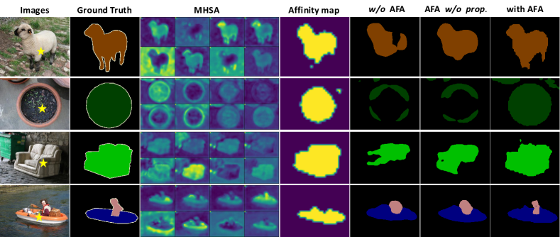
Figure 4: Visualization of the MHSA maps, learned affinity maps, and generated pseudo labels for segmentation. ”$\bigstar$” denotes the query point to visualize the attention and affinity maps.

Table 3: Evaluation of the pseudo labels for segmentation.

		$train$	$val$
PSA [2]		59.7	–
IRN [1]		66.5	–
1Stage [4]		66.9	65.3
Ours	w/o AFA	54.4	54.2
	AFA (w/o $prop.$)	66.3	64.4
	AFA ($prop.$ with MHSA)	58.3	55.9
	AFA	68.7	66.5

AFA. The motivation of AFA is to learn reliable semantic affinity from MHSA and revise the pseudo labels with the learned affinity. In Fig. 4, we present some example images of the self-attention maps (extracted from the last Transformer block) and the learned affinity maps. Fig. 4 shows that our AFA could effectively learn reliable semantic affinity from the inaccurate MHSA. The affinity loss in the AFA module also encourages the MHSA to model the semantic relations well. In Fig. 4, we also present the pseudo labels generated from our model without AFA module (w/o AFA), with AFA module but no random walk propagation (AFA w/o $prop.$) and with full AFA module. For the generated pseudo labels, the AFA module brings notable visual improvements. The affinity propagation process further diffuses the regions with high semantic affinity and dampens the regions with low affinity.

In Tab. 3, we report the quantitative results of the generated pseudo labels on PASCAL VOC $train$ and $val$ set. We also report the results of performing random walk propagation with the average vanilla MHSA as semantic affinity (AFA $prop.$ with MHSA). The results show that the affinity learning loss in the AFA module remarkably improves the accuracy of the pseudo labels (from 54.4% mIoU to 66.3% mIoU on the $train$ set). The propagation process could further promote the reliability of pseudo labels, which harvests the performance gains in Tab. 2. It is also noted that propagation with the naive MHSA significantly reduces the accuracy, demonstrating our motivation and the effectiveness of the AFA module.

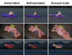
Figure 5: Examples of PAR’s improvements on the pseudo labels. The pseudo labels are generated with CAM and Transformer baseline.

PAR. The proposed PAR aims at refining the initial pseudo labels with low-level image appearance and position information. In Fig. 5, we present the qualitative improvements of PAR. Fig. 5 shows PAR effectively dampens the falsely activated regions, enforcing better alignment with the low-level boundaries.

Quantitatively, as shown in Tab. 4, our PAR improves the CAM (generated with Transformer baseline) from 48.2% to 52.9%, which outperforms PAMR [4], which is also based on the dilated pixel-adaptive convolution to incorporate local image appearance information. Tab. 4 also demonstrates the position kernel $\kappa_{pos}$ in PAR is beneficial for refining CAM. More investigation details on PAR are presented in the supplementary material.

Table 4: Comparison of refinement methods for CAM.

	$\kappa_{rgb}$	$\kappa_{pos}$	$train$
CAM			48.2
PAMR [4]	✓		51.4
PAR	✓		51.7
	✓	✓	52.9

Table 5: Semantic segmentation results on PASCAL VOC 2012 dataset. $Sup.$ denotes supervision type. $\mathcal{F}$: full supervision; $\mathcal{I}$: image-level labels; $\mathcal{S}$: saliency maps. $\dagger$ denotes our implementation.

Method	$Sup.$	Backbone	$val$	$test$
Fully-supervised models.
DeepLab [8]	$\mathcal{F}$	R101	77.6	79.7
WideResNet38 [48]		WR38	80.8	82.5
Segformer † [49]		MiT-B1	78.7	–
Multi-Stage weakly-supervised models.
OAA+ [16] ICCV’2019	$\mathcal{I}+\mathcal{S}$	R101	65.2	66.4
MCIS [39] ECCV’2020		R101	66.2	66.9
AuxSegNet [50] ICCV’2021		WR38	69.0	68.6
NSROM [51] CVPR’2021		R101	70.4	70.2
EPS [25] CVPR’2021		R101	70.9	70.8
SEAM [45] CVPR’2020	$\mathcal{I}$	WR38	64.5	65.7
SC-CAM [7] CVPR’2020		R101	66.1	65.9
CDA [38] ICCV’2021		WR38	66.1	66.8
AdvCAM [23] CVPR’2021		R101	68.1	68.0
CPN [56] ICCV’2021		R101	67.8	68.5
RIB [22] NeurIPS’2021		R101	68.3	68.6
End-to-End weakly-supervised models.
EM [31] ICCV’2015	$\mathcal{I}$	VGG16	38.2	39.6
MIL [32] CVPR’2015		–	42.0	40.6
CRF-RNN [34] CVPR’2017		VGG16	52.8	53.7
RRM [53] AAAI’2020		WR38	62.6	62.9
RRM † [53] AAAI’2020		MiT-B1	63.5	–
1Stage [4] CVPR’2020		WR38	62.7	64.3
AA&LR [57] ACM MM’2021		WR38	63.9	64.8
Ours		MiT-B1	66.0	66.3

4.4 Comparison to State-of-the-art

PASCAL VOC 2012. We report the semantic segmentation performance on PASCAL VOC 2012 $val$ and $test$ set in Tab. 5. R101 and WR38 denote the method uses ResNet101 [15] and WideResNet38 [48] as backbone, respectively. Tab. 5 shows that the proposed model clearly surpasses previous state-of-the-art end-to-end methods. Our method achieves 83.8% of its fully-supervised counterpart, , Segformer [49], while 1Stage [4] and AA&LR [57] only achieve 77.6% and 79.1% of WideResNet38, respectively. Our method is also competitive with some recent multi-stage WSSS methods, such as OAA+ [16], SEAM [45], SC-CAM [7], and CDA [38]. It’s also noted that our method also outperforms RRM with MiT-B1 as backbone, which demonstrates the efficay of the proposed AFA and PAR.

MS COCO 2014. We present the semantic segmentation performance on the challenging MS COCO 2014 dataset in Tab. 6. Our end-to-end method could achieve 38.9% mIoU on the $val$ set, which remarkably outperforms most recent multi-stage methods (except RIB [22]).

Table 6: Semantic segmentation results on MS COCO dataset.

Method	$Sup.$	Backbone	$val$
Multi-Stage weakly-supervised models.
EPS [25] CVPR’2021	$\mathcal{I}+\mathcal{S}$	R101	35.7
AuxSegNet [50] ICCV’2021		WR38	33.9
SEAM [45] CVPR’2020	$\mathcal{I}$	WR38	31.9
CONTA [55] NeurIPS’2020		WR38	32.8
CDA [38] ICCV’2021		WR38	31.7
CGNet [21] ICCV’2021		WR38	36.4
RIB [22] NeurIPS’2021		R101	43.8
End-to-End weakly-supervised models.
Ours		MiT-B1	38.0
Ours + CRF	$\mathcal{I}$	MiT-B1	38.9

Qualitative Results. In Fig. 6, we present the qualitative results of our method on the PASCAL VOC and MS COCO $val$ set. On the PASCAL VOC dataset, visually, our method could outperform 1Stage [4] and produce segmentation results that align finely with object boundaries. The qualitative results on MS COCO dataset are also comparable with the ground truth.

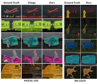
Figure 6: Segmentation results of 1Stage [4] and our method on VOC and COCO $val$ set.

5 Conclusion

In this work, we explore the intrinsic virtue of Transformer architecture for WSSSS tasks. Specifically, we use a Transformer-based backbone to generate CAM as the initial pseudo labels, avoiding the inherent flaw of CNN. Besides, we note the consistency between the MHSA and semantic affinity, and thus propose the AFA module. AFA derives reliable affinity labels from pseudo labels, imposes the affinity labels to supervise the MHSA, and produces reliable affinity predictions. The learned affinity is used to revise the initial pseudo labels via random walk propagation. On PASCAL VOC and MS COCO datasets, our method achieves new state-of-the-art performance for end-to-end WSSS. In a broader view, the proposed method also shows a novel perspective for vision transformers, guiding the self-attention with semantic relation to ensure better feature aggregation.

6 More Technical Details

6.1 Details of Backbone

We use the MiT-B1 proposed in SegFormer [49] as the backbone, which is a more friendly backbone for image segmentation tasks than the vanilla ViT [11]. SegFormer uses Overlapped Patch Merging layers with different strides to produce multi-scale feature maps. As shown in Fig. 7, in SegFormer, the feature of Stage #4 is $\frac{h}{32}\times\frac{w}{32}$. To obtain the initial pseudo labels (CAM) with higher resolution, we change the stride of the last patch merging layer from 2 to 1, increasing resolution of the feature maps to the size of $\frac{h}{16}\times\frac{w}{16}$.

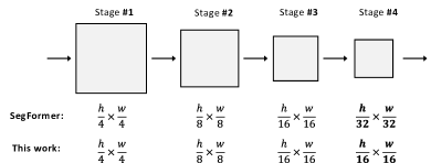
Figure 7: The size of feature maps of different stags.

In practice, to produce the semantic affinity prediction, we use the multi-head self-attention (MHSA) matrices extracted from the last stage, which could capture the high-level semantic information. The MHSA matrices are concatenated to form $S\in\mathbb{R}^{\frac{hw}{256}\times\frac{hw}{256}\times nk}$ and prediction the semantic affinity, where $n$ and $k$ are the number of Transformer blocks and heads in each block, respectively.

6.2 Mask for Affinity Loss

Inspired by [1, 2], when computing affinity loss, we only consider the situation that pixel pairs are in the same local window with the radius of $r$, and disregard their affinity if the distance is too far. Specifically, given a pixel $(i,j)$, if pixel $(k,l)$ is the same window with $(i,j)$, their affinity is computed; otherwise, their affinity is ignored. Unlike [1, 2], which extract pixel pairs when computing affinity loss, we efficiently implemented by applying a mask. The conceptual illustration of this strategy and an example mask is presented in Fig. 8.

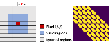
Figure 8: Left: Illustration of the valid pixel pairs. Right: Example mask for computing the affinity loss.

7 More Experimental Results

7.1 Hyper-parameters

Affinity from Attention. In Tab. 7, we present segmentation results on the PASCAL VOC $val$ set with different radius $r$ of the local window size when computing the affinity loss. Intuitively, a small $r$ can not provide enough affinity pairs while a large $r$ may not ensure the reliability of distant affinity pairs. As shown in Tab. 7, $r=8$ is a proper choice.

Table 7: Impact of the radius $r$ when computing the affinity loss. The results are evaluated on the $val$ set of PASCAL VOC 2012.

radius $r$	2	4	8	12	16
$val$	62.4	62.7	63.8	61.5	59.4

Pixel-Adaptive Refinement. In Tab. 8, we report the impact of different configurations of the proposed Pixel-Adaptive Refinement, including the dilation rates, position kernel, and the number of iteration. Tab. 8 shows that for the same dilation rates, our PAR remarkably outperforms PAMR [4], demonstrating the necessity of the position kernel.

Table 8: Ablation of the dilation rates, position kernel and number of iteration of the proposed PAR. The results are evaluated on the $train$ set of PASCAL VOC 2012 in mIoU (%).

	Dilations						$\kappa_{pos}$	Iter	$train$
	1	2	4	8	12	24
CAM									48.2
PAMR[4]	✓	✓	✓	✓	✓	✓			51.4
CRF									54.5
PAR	✓	✓	✓				✓	15	48.8
	✓	✓	✓	✓			✓	15	49.9
	✓	✓	✓	✓	✓		✓	15	51.3
	✓	✓	✓	✓	✓	✓		15	51.5
	✓	✓	✓	✓	✓	✓	✓	15	52.9
	✓	✓	✓	✓	✓	✓	✓	20	52.9

Tab. 9 presents the impact of the weights factors of PAR. For simplicity, we set $w_{1}=w_{2}$. Tab. 9 shows $w_{1}=0.3,w_{2}=0.3,w_{3}=0.01$ is a favorable choice.

Table 9: Ablation of weight factors of the proposed PAR. The results are evaluated on the $train$ set of PASCAL VOC 2012.

		$w_{3}$
		0.005	0.01	0.02	0.03
$w_{1}$ & $w_{2}$	0.1	51.9	51.7	50.1	–
	0.3	52.8	52.9	51.4	48.4
	0.5	51.9	52.5	51.3	48.3
	0.7	–	51.6	50.9	48.0

Weight Factors. We present the segmentation results on the PASCAL VOC $val$ set with different weight factors of loss terms in Tab. 10. $\lambda_{1}=0.1,\lambda_{2}=0.2,\lambda_{2}=0.01$ is a preferred choice for our framework.

Table 10: Impact of the weights of loss terms. The results are evaluated on the $val$ set of PASCAL VOC 2012.

	$\lambda_{1}$	$\lambda_{2}$	$\lambda_{3}$	$val$
Default	0.1	0.1	0.01	63.8
	0.05			62.8
	0.2			61.6
	0.5			57.8
		0.05		63.4
		0.2		61.7
		0.5		58.7
			0.005	62.4
			0.02	62.3
			0.05	61.5

Background Scores We investigate the impact of the background scores $(\beta_{l},\beta_{h})$ to filter the pseudo labels to the reliable foreground, background, and uncertain regions. Intuitively, large $\beta_{h}$ and small $\beta_{l}$ could produce more reliable pseudo labels but reduce the number of valid labels. On the contrary, small $\beta_{h}$ and large $\beta_{l}$ will introduce noise to the pseudo labels. Note that the average value of $\beta_{h}$ and $\beta_{l}$ is always 0.45, which is the preferred background score for generated CAM in our preliminary experiments.

Table 11: Impact of the background scores $\beta_{h},\beta_{l}$. The results are evaluated on the $val$ set of PASCAL VOC 2012.

	$\beta_{h}$	$\beta_{l}$	$val$
	0.65	0.25	60.7
	0.6	0.3	62.5
Default	0.55	0.35	63.8
	0.5	0.4	62.9
	0.45	0.45	60.5

Table 12: Evaluation and comparison of the semantic segmentation results in mIoU on the $val$ set.

	RRM[53]	1Stage [4]	AA&LR [57]	Ours
bkg	87.9	88.7	88.4	89.9
aero	75.9	70.4	76.3	79.5
bicycle	31.7	35.1	33.8	31.2
bird	78.3	75.7	79.9	80.7
boat	54.6	51.9	34.2	67.2
bottle	62.2	65.8	68.2	61.9
bus	80.5	71.9	75.8	81.4
car	73.7	64.2	74.8	65.4
cat	71.2	81.1	82.0	82.3
chair	30.5	30.8	31.8	28.7
cow	67.4	73.3	68.7	83.4
table	40.9	28.1	47.4	41.6
dog	71.8	81.6	79.1	82.2
horse	66.2	69.1	68.5	75.9
motor	70.3	62.6	71.4	70.2
person	72.6	74.8	80.0	69.4
plant	49.0	48.6	50.3	53.0
sheep	70.7	71.0	76.5	85.9
sofa	38.4	40.1	43.0	44.1
train	62.7	68.5	55.5	64.2
tv	58.4	64.3	58.5	50.9
mIOU	62.6	62.7	63.9	66.0

7.2 More Quantitative Results

We present the per-category segmentation results on PASCAL VOC $val$ set in Tab 12. Our method achieves the best results for most categories. The results on $test$ set are available at the official PASCAL VOC evaluation website.

7.3 More Qualitative Results

We present more qualitative results as follows.

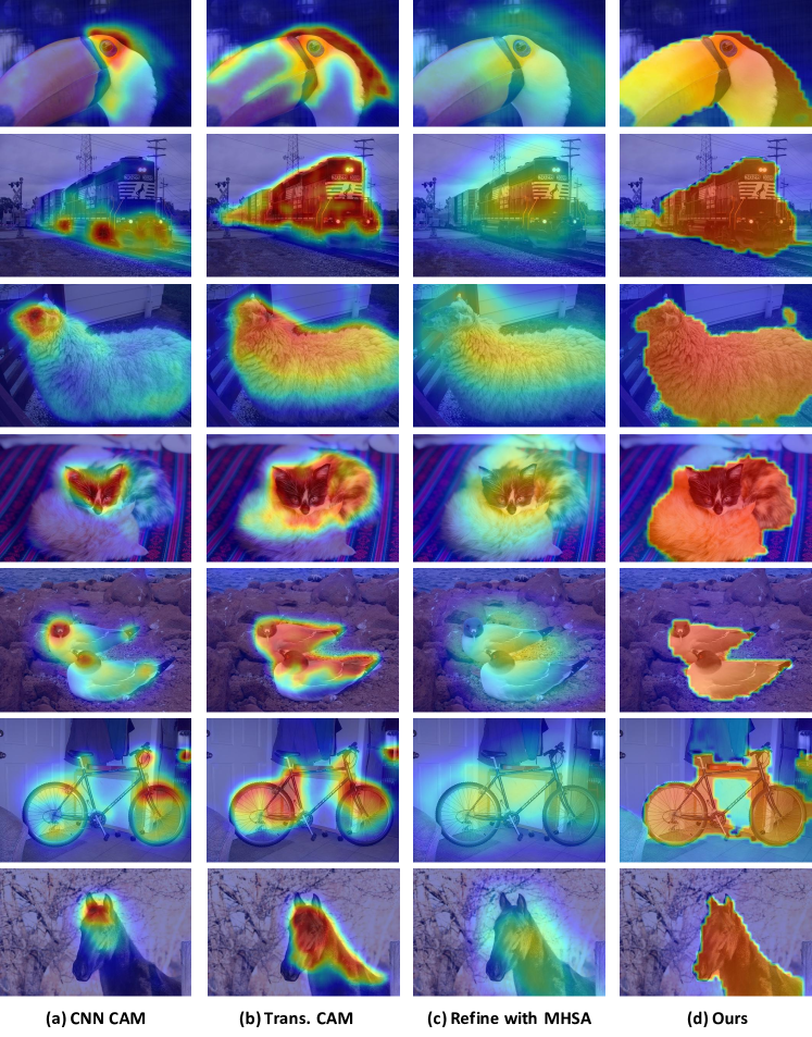
Figure 9: CAM generated with (a) Transformers activates more integral regions than (b) CNN. Refining CAM with (c) coarse MHSA doesn’t work well, while (d) the learned affinity could remarkably improve the generated CAM.

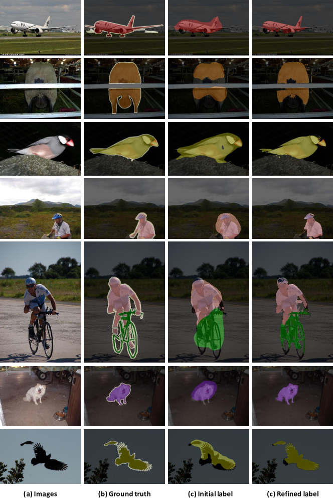
Figure 10: Improvements of the proposed pixel-adaptive refinement (PAR) module on the pseudo labels. The pseudo labels are generated with CAM and Transformer baseline. The proposed PAR could effectively dampen the falsely activated regions and ensure the alignment with low-level image appearance.

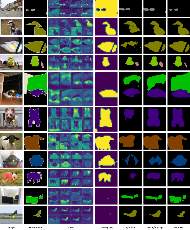
Figure 11: Visualization of the MHSA maps, learned affinity maps, and generated pseudo labels for segmentation. ”$\bigstar$” denotes the query point to visualize the attention and affinity maps. The pseudo labels are generated with our model without AFA module (w/o AFA), with AFA module but no random walk propagation (AFA w/o $prop.$) and with full AFA module (with AFA). For the generated pseudo labels, the AFA module brings notable visual improvements. The affinity propagation process further diffuses the regions with high semantic affinity and dampens the regions with low affinity.

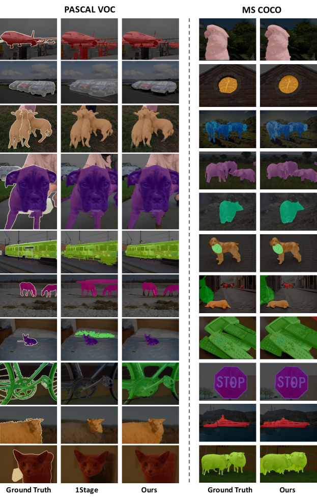
Figure 12: Semantic segmentation results on PASCAL VOC $val$ (left) and MS COCO $val$ set (right). Our method outperforms 1Stage [4] and is comparable with ground truth labels.

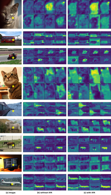
Figure 13: Visualization of the MHSA maps extracted from model without and with our AFA. ”$\bigstar$” denotes the query point. Our AFA could help the MHSA to capture better semantic affinity.

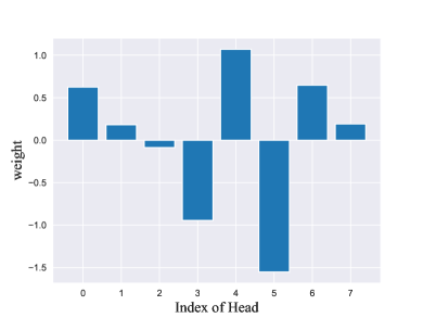
Figure 14: The learned weights of each head of self-attention in the AFA module. Here we only present the 8 heads of the last Transformer block. The MHSA matrices do not contribute equally to semantic affinity. Some self-attention matrices (head #2, head #3, and head #5) contribute negatively to semantic affinity. The learned weights suggest applying MHSA directly as semantic affinity is not beneficial for the pseudo labels.

References

- [1] Jiwoon Ahn, Sunghyun Cho, and Suha Kwak. Weakly supervised learning of instance segmentation with inter-pixel relations. In CVPR, pages 2209–2218, 2019.
- [2] Jiwoon Ahn and Suha Kwak. Learning pixel-level semantic affinity with image-level supervision for weakly supervised semantic segmentation. In CVPR, pages 4981–4990, 2018.
- [3] Peri Akiva and Kristin Dana. Towards single stage weakly supervised semantic segmentation. arXiv preprint arXiv:2106.10309, 2021.
- [4] Nikita Araslanov and Stefan Roth. Single-stage semantic segmentation from image labels. In CVPR, pages 4253–4262, 2020.
- [5] Anurag Arnab, Mostafa Dehghani, Georg Heigold, Chen Sun, Mario Lučić, and Cordelia Schmid. Vivit: A video vision transformer. ICCV, 2021.
- [6] Jimmy Lei Ba, Jamie Ryan Kiros, and Geoffrey E Hinton. Layer normalization. arXiv preprint arXiv:1607.06450, 2016.
- [7] Yu-Ting Chang, Qiaosong Wang, Wei-Chih Hung, Robinson Piramuthu, Yi-Hsuan Tsai, and Ming-Hsuan Yang. Weakly-supervised semantic segmentation via sub-category exploration. In CVPR, pages 8991–9000, 2020.
- [8] Liang-Chieh Chen, George Papandreou, Iasonas Kokkinos, Kevin Murphy, and Alan L Yuille. Deeplab: Semantic image segmentation with deep convolutional nets, atrous convolution, and fully connected crfs. TPAMI, 40(4):834–848, 2017.
- [9] Bowen Cheng, Alexander G Schwing, and Alexander Kirillov. Per-pixel classification is not all you need for semantic segmentation. arXiv preprint arXiv:2107.06278, 2021.
- [10] Jia Deng, Wei Dong, Richard Socher, Li-Jia Li, Kai Li, and Li Fei-Fei. Imagenet: A large-scale hierarchical image database. In CVPR, pages 248–255, 2009.
- [11] Alexey Dosovitskiy, Lucas Beyer, Alexander Kolesnikov, Dirk Weissenborn, Xiaohua Zhai, Thomas Unterthiner, Mostafa Dehghani, Matthias Minderer, Georg Heigold, Sylvain Gelly, et al. An image is worth 16x16 words: Transformers for image recognition at scale. In ICLR, 2020.
- [12] Mark Everingham, Luc Van Gool, Christopher KI Williams, John Winn, and Andrew Zisserman. The pascal visual object classes (voc) challenge. IJCV, 88(2):303–338, 2010.
- [13] Wei Gao, Fang Wan, Xingjia Pan, Zhiliang Peng, Qi Tian, Zhenjun Han, Bolei Zhou, and Qixiang Ye. Ts-cam: Token semantic coupled attention map for weakly supervised object localization. In ICCV, pages 2886–2895, October 2021.
- [14] Bharath Hariharan, Pablo Arbeláez, Lubomir Bourdev, Subhransu Maji, and Jitendra Malik. Semantic contours from inverse detectors. In 2011 International Conference on Computer Vision, pages 991–998, 2011.
- [15] Kaiming He, Xiangyu Zhang, Shaoqing Ren, and Jian Sun. Deep residual learning for image recognition. In CVPR, pages 770–778, 2016.
- [16] Peng-Tao Jiang, Qibin Hou, Yang Cao, Ming-Ming Cheng, Yunchao Wei, and Hong-Kai Xiong. Integral object mining via online attention accumulation. In ICCV, pages 2070–2079, 2019.
- [17] Tsung-Wei Ke, Jyh-Jing Hwang, Ziwei Liu, and Stella X Yu. Adaptive affinity fields for semantic segmentation. In ECCV, pages 587–602, 2018.
- [18] Beomyoung Kim, Sangeun Han, and Junmo Kim. Discriminative region suppression for weakly-supervised semantic segmentation. In AAAI, volume 35, pages 1754–1761, 2021.
- [19] Alexander Kolesnikov and Christoph H Lampert. Seed, expand and constrain: Three principles for weakly-supervised image segmentation. In ECCV, pages 695–711. Springer, 2016.
- [20] Philipp Krähenbühl and Vladlen Koltun. Efficient inference in fully connected crfs with gaussian edge potentials. NeurIPS, 24:109–117, 2011.
- [21] Hyeokjun Kweon, Sung-Hoon Yoon, Hyeonseong Kim, Daehee Park, and Kuk-Jin Yoon. Unlocking the potential of ordinary classifier: Class-specific adversarial erasing framework for weakly supervised semantic segmentation. In ICCV, pages 6994–7003, 2021.
- [22] Jungbeom Lee, Jooyoung Choi, Jisoo Mok, and Sungroh Yoon. Reducing information bottleneck for weakly supervised semantic segmentation. NeurIPS, 34, 2021.
- [23] Jungbeom Lee, Eunji Kim, and Sungroh Yoon. Anti-adversarially manipulated attributions for weakly and semi-supervised semantic segmentation. In CVPR, pages 4071–4080, 2021.
- [24] Jungbeom Lee, Jihun Yi, Chaehun Shin, and Sungroh Yoon. Bbam: Bounding box attribution map for weakly supervised semantic and instance segmentation. In CVPR, pages 2643–2652, 2021.
- [25] Seungho Lee, Minhyun Lee, Jongwuk Lee, and Hyunjung Shim. Railroad is not a train: Saliency as pseudo-pixel supervision for weakly supervised semantic segmentation. In CVPR, pages 5495–5505, 2021.
- [26] Xueyi Li, Tianfei Zhou, Jianwu Li, Yi Zhou, and Zhaoxiang Zhang. Group-wise semantic mining for weakly supervised semantic segmentation. In AAAI, volume 35, pages 1984–1992, 2021.
- [27] Yi Li, Zhanghui Kuang, Liyang Liu, Yimin Chen, and Wayne Zhang. Pseudo-mask matters inweakly-supervised semantic segmentation. ICCV, 2021.
- [28] Di Lin, Jifeng Dai, Jiaya Jia, Kaiming He, and Jian Sun. Scribblesup: Scribble-supervised convolutional networks for semantic segmentation. In CVPR, pages 3159–3167, 2016.
- [29] Tsung-Yi Lin, Michael Maire, Serge Belongie, James Hays, Pietro Perona, Deva Ramanan, Piotr Dollár, and C Lawrence Zitnick. Microsoft coco: Common objects in context. In ECCV, pages 740–755. Springer, 2014.
- [30] Ilya Loshchilov and Frank Hutter. Decoupled weight decay regularization. In ICLR, 2019.
- [31] George Papandreou, Liang-Chieh Chen, Kevin P Murphy, and Alan L Yuille. Weakly-and semi-supervised learning of a deep convolutional network for semantic image segmentation. In ICCV, pages 1742–1750, 2015.
- [32] Pedro O Pinheiro and Ronan Collobert. From image-level to pixel-level labeling with convolutional networks. In CVPR, pages 1713–1721, 2015.
- [33] René Ranftl, Alexey Bochkovskiy, and Vladlen Koltun. Vision transformers for dense prediction. In ICCV, pages 12179–12188, 2021.
- [34] Anirban Roy and Sinisa Todorovic. Combining bottom-up, top-down, and smoothness cues for weakly supervised image segmentation. In CVPR, pages 3529–3538, 2017.
- [35] Lixiang Ru, Bo Du, and Chen Wu. Learning visual words for weakly-supervised semantic segmentation. In IJCAI, pages 982–988, 8 2021.
- [36] Lixiang Ru, Bo Du, Yibing Zhan, and Chen Wu. Weakly-supervised semantic segmentation with visual words learning and hybrid pooling. IJCV, 2022.
- [37] Hang Su, Varun Jampani, Deqing Sun, Orazio Gallo, Erik Learned-Miller, and Jan Kautz. Pixel-adaptive convolutional neural networks. In CVPR, pages 11166–11175, 2019.
- [38] Yukun Su, Ruizhou Sun, Guosheng Lin, and Qingyao Wu. Context decoupling augmentation for weakly supervised semantic segmentation. pages 7004–7014, October 2021.
- [39] Guolei Sun, Wenguan Wang, Jifeng Dai, and Luc Van Gool. Mining cross-image semantics for weakly supervised semantic segmentation. In ECCV, pages 347–365. Springer, 2020.
- [40] Kunyang Sun, Haoqing Shi, Zhengming Zhang, and Yongming Huang. Ecs-net: Improving weakly supervised semantic segmentation by using connections between class activation maps. In ICCV, pages 7283–7292, 2021.
- [41] Meng Tang, Federico Perazzi, Abdelaziz Djelouah, Ismail Ben Ayed, Christopher Schroers, and Yuri Boykov. On regularized losses for weakly-supervised cnn segmentation. In ECCV, pages 507–522, 2018.
- [42] Ashish Vaswani, Noam Shazeer, Niki Parmar, Jakob Uszkoreit, Llion Jones, Aidan N Gomez, Łukasz Kaiser, and Illia Polosukhin. Attention is all you need. In NeurIPS, pages 5998–6008, 2017.
- [43] Petar Veličković, Guillem Cucurull, Arantxa Casanova, Adriana Romero, Pietro Liò, and Yoshua Bengio. Graph attention networks. In ICLR, 2018.
- [44] Paul Vernaza and Manmohan Chandraker. Learning random-walk label propagation for weakly-supervised semantic segmentation. In CVPR, pages 7158–7166, 2017.
- [45] Yude Wang, Jie Zhang, Meina Kan, Shiguang Shan, and Xilin Chen. Self-supervised equivariant attention mechanism for weakly supervised semantic segmentation. In CVPR, pages 12275–12284, 2020.
- [46] Yunchao Wei, Jiashi Feng, Xiaodan Liang, Ming-Ming Cheng, Yao Zhao, and Shuicheng Yan. Object region mining with adversarial erasing: A simple classification to semantic segmentation approach. In CVPR, pages 1568–1576, 2017.
- [47] Tong Wu, Junshi Huang, Guangyu Gao, Xiaoming Wei, Xiaolin Wei, Xuan Luo, and Chi Harold Liu. Embedded discriminative attention mechanism for weakly supervised semantic segmentation. In CVPR, pages 16765–16774, 2021.
- [48] Zifeng Wu, Chunhua Shen, and Anton Van Den Hengel. Wider or deeper: Revisiting the resnet model for visual recognition. PR, 90:119–133, 2019.
- [49] Enze Xie, Wenhai Wang, Zhiding Yu, Anima Anandkumar, Jose M Alvarez, and Ping Luo. Segformer: Simple and efficient design for semantic segmentation with transformers. arXiv preprint arXiv:2105.15203, 2021.
- [50] Lian Xu, Wanli Ouyang, Mohammed Bennamoun, Farid Boussaid, Ferdous Sohel, and Dan Xu. Leveraging auxiliary tasks with affinity learning for weakly supervised semantic segmentation. In ICCV, pages 6984–6993, October 2021.
- [51] Yazhou Yao, Tao Chen, Guo-Sen Xie, Chuanyi Zhang, Fumin Shen, Qi Wu, Zhenmin Tang, and Jian Zhang. Non-salient region object mining for weakly supervised semantic segmentation. In CVPR, pages 2623–2632, 2021.
- [52] Bingfeng Zhang, Jimin Xiao, Jianbo Jiao, Yunchao Wei, and Yao Zhao. Affinity attention graph neural network for weakly supervised semantic segmentation. TPAMI, 2021.
- [53] Bingfeng Zhang, Jimin Xiao, Yunchao Wei, Mingjie Sun, and Kaizhu Huang. Reliability does matter: An end-to-end weakly supervised semantic segmentation approach. In AAAI, number 07, pages 12765–12772, 2020.
- [54] Bingfeng Zhang, Jimin Xiao, and Yao Zhao. Dynamic feature regularized loss for weakly supervised semantic segmentation. arXiv preprint arXiv:2108.01296, 2021.
- [55] Dong Zhang, Hanwang Zhang, Jinhui Tang, Xian-Sheng Hua, and Qianru Sun. Causal intervention for weakly-supervised semantic segmentation. NeurIPS, 33, 2020.
- [56] Fei Zhang, Chaochen Gu, Chenyue Zhang, and Yuchao Dai. Complementary patch for weakly supervised semantic segmentation. In ICCV, pages 7242–7251, 2021.
- [57] Xiangrong Zhang, Zelin Peng, Peng Zhu, Tianyang Zhang, Chen Li, Huiyu Zhou, and Licheng Jiao. Adaptive affinity loss and erroneous pseudo-label refinement for weakly supervised semantic segmentation. In ACM MM, 2021.
- [58] Sixiao Zheng, Jiachen Lu, Hengshuang Zhao, Xiatian Zhu, Zekun Luo, Yabiao Wang, Yanwei Fu, Jianfeng Feng, Tao Xiang, Philip HS Torr, et al. Rethinking semantic segmentation from a sequence-to-sequence perspective with transformers. In CVPR, pages 6881–6890, 2021.
- [59] Bolei Zhou, Aditya Khosla, Agata Lapedriza, Aude Oliva, and Antonio Torralba. Learning deep features for discriminative localization. In CVPR, pages 2921–2929, 2016.