Theoretical results and modeling under the discrete Birnbaum-Saunders distribution

Abstract

In this paper, we discuss some theoretical results and properties of a discrete version of the Birnbaum-Saunders distribution. We present a proof of the unimodality of this model. Moreover, results on moments, quantile function, reliability and order statistics are also presented. In addition, we propose a regression model based on the discrete Birnbaum-Saunders distribution. The model parameters are estimated by the maximum likelihood method and a Monte Carlo study is performed to evaluate the performance of the estimators. Finally, we illustrate the proposed methodology with the use of real data sets.

Keywords

Birnbaum-Saunders distribution; Regression model; Maximum likelihood; Monte Carlo simulation; R software.

1 Introduction

Despite the increasing number of works on discrete distributions in reliability, one can note that in many practical cases there is the need of more flexible distributions to model lifetime data. One way to develop new discrete distributions is by generating the discrete analogous of usual distributions for continuous lifetimes; see Alzaatreh et al., (2012). Some interesting discrete distributions are for example the discrete gamma distribution (Abouammoh and Alhazzani,, 2015) and the discrete Weibull distribution (Vila et al.,, 2019). It is well known that in reliability, the continuous Birnbaum-Saunders (BS) distribution, proposed by Birnbaum and Saunders, (1969), takes advantage than most continuous probability distributions, including the continuous gamma and Weibull distributions; see Leiva, (2016). The continuous BS distribution is a positively skewed model that is closely related to the normal distribution. Despite its origin in material fatigue, it has been considered in business, industry, insurance, inventory, quality control, among others; see, for example, Lio and Park, (2008), Balakrishnan et al., (2009), Ahmed et al., (2010), Vilca et al., (2010), Paula et al., (2012), Marchant et al., (2013), Rojas et al., (2015), Wanke and Leiva, (2015), Leiva et al., (2011); Leiva et al., 2014a ; Leiva et al., 2014b ; Leiva et al., (2017), Saulo et al., (2019), Desousa et al., (2018), Leão et al., (2018), and Ventura et al., (2019). Good recent references on the Birnbaum-Saunders distribution are Leiva, (2016) and Balakrishnan and Kundu, (2019). In particular, a positive random variable $T$ is said to follow a continuous BS distribution if its cumulative distribution function (CDF) is given by

$$F_{T}(t;\bm{\theta})=\Phi\left[a(t;\bm{\theta})\right],\,t>0,$$ (1)

where $\bm{\theta}=(\alpha,\beta)^{\top}$, with $\alpha>0$ and $\beta>0$ denoting the shape and scale parameters, respectively, $a(t;\bm{\theta})=\big{(}\sqrt{{t}/{\beta}}-\sqrt{{\beta}/{t}}\big{)}/\alpha$, and $\Phi[\cdot]$ is the standard normal CDF. This distribution is usually denoted by $T\sim{\rm BS}(\bm{\theta})$. Even though the number of applications of the usual continuous BS distribution has been growing, there is a big number of applications where a discrete version of this distribution could be more appropriate. For example, to model the number of cycles or runs that a material or equipment supports before failing or breaking, the number of sessions of a treatment until the cure of a patient, or even the shelf life (in days) of a food product; see Vila et al., (2019).

In this paper, we study in more depth a discrete version of the continuous BS distribution, which was initially introduced by Sen et al., (2010). The primary objectives of this paper are: (i) to discuss novel theoretical results and properties of this discrete BS (${\rm BS_{d}}$) distribution; and (ii) to introduce the corresponding regression model. The secondary objectives are: (i) to obtain the maximum likelihood estimates of the model parameters; (ii) to carry out Monte Carlo simulations to evaluate the performance of the maximum likelihood estimators; and (iv) to discuss real data applications of the proposed methodology.

The rest of the paper proceeds as follows. In Section 2, we present the ${\rm BS_{d}}$ model and discuss some of its mathematical properties. Also, it is considered estimation of the model parameters based on maximum likelihood method. In Section 3, a ${\rm BS_{d}}$ regression model is proposed, and the model parameter estimation is approached by using the maximum likelihood method. In Section  4, we carry out Monte Carlo simulation studies to evaluate the performance of the estimators and we illustrate the proposed methodology with two real data sets. Finally, in Section 5, we make some concluding remarks.

2 Discrete Birnbaum-Saunders distribution

Before defining the proposed discrete distribution, we present the probability density function (PDF) and quantile function of the continuous BS distribution. If $T\sim{\rm BS}(\bm{\theta})$, then its PDF is given by

$$f_{T}(t;\bm{\theta})=\phi\big{[}a(t;\bm{\theta})\big{]}a^{\prime}(t;\bm{\theta}),\,t>0,$$

where $\phi[\,\cdot\,]$ is the PDF of the standard normal distribution, $a(t;\bm{\theta})$ is as in (1) and $a^{\prime}(t;\bm{\theta})=(t+\beta)/(2t^{3/2}\alpha\beta^{1/2})$ is the derivative of $a(t;\bm{\theta})$ with respect to $t$. Moreover, the $p$-th quantile of $T\sim{\rm BS}(\bm{\theta})$ is given by

$$Q_{p}={\beta\over 4}\,\left\{\alpha\Phi^{-1}(p)+\sqrt{[\alpha\Phi^{-1}(p)]^{2}+4}\right\}^{2},$$ (2)

where $p\in(0,1)$.

Now, we are ready to present a discrete random variable associated to the positive $T$ as follows $S=\lfloor T\rfloor,$ where $\lfloor t\rfloor$ denotes the largest integer contained in $t$. As the set of all possible values of $T$ is the set $(0,\infty)$, then $S=s$ iff $s<T\leq s+1,\,s=0,1,\ldots.$ Consequently, the probability mass function (PMF) of $S$ can be expressed by

$$\mathbb{P}(S=s)=\mathbb{P}(s<T\leq s+1)=\begin{cases}\Phi\big{[}a(1;\bm{\theta})\big{]},&\text{if}\ s=0,\\[5.69046pt] \Phi\big{[}a(s+1;\bm{\theta})\big{]}-\Phi\big{[}a(s;\bm{\theta})\big{]},&\text{if}\ s=1,2,\ldots,\end{cases}$$ (3)

where $a(\cdot;\bm{\theta})$ is as in (1). We can show that $\sum_{s=0}^{\infty}\mathbb{P}(S=s)=\mathbb{P}(T>0)=1$, so $\mathbb{P}(S=s)$ is a PMF. On the other hand, the CDF of $S$ is given by

$${F}(s;\bm{\theta})=\mathbb{P}(S\leq s)=\Phi\big{[}a(\lfloor s\rfloor+1;\bm{\theta})\big{]}\mathds{1}_{\{s\geq 0\}}.$$

The distribution of the discrete random variable $S$ will be denoted by $S\sim{\rm BS_{d}}(\bm{\theta})$ and will be called ${\rm BS_{d}}$ distribution.

The reliability function (RF) and hazard rate function (HR) of $S\sim{\rm BS_{d}}(\bm{\theta})$ are, respectively, given by

$$R(s;\bm{\theta})=1-F(s;\bm{\theta})=1-\Phi\big{[}a({\lfloor s\rfloor}+1;\bm{\theta})\big{]}\mathds{1}_{\{s\geq 0\}},$$ (4)

$${H}(s;\bm{\theta})={\mathbb{P}(S=s)\over\mathbb{P}(S=s)+R(s;\bm{\theta})} =\begin{cases}\Phi\big{[}a({1};\bm{\theta})\big{]},&\text{if}\ s=0,\\[5.69046pt] {\Phi[a({s+1};\bm{\theta})]-\Phi[a({s};\bm{\theta})]\over 1-\Phi[a({s};\bm{\theta})]}&\text{if}\ s=1,2,\ldots,\end{cases}$$

$$=\begin{cases}1-R(0;\bm{\theta}),&\text{if}\ s=0,\\[5.69046pt] 1-{R(s;\bm{\theta})\over R(s-1;\bm{\theta})},&\text{if}\ s=1,2,\ldots.\end{cases}$$

From the above identity, we have

$$R(s;\bm{\theta})=\prod_{y=0}^{s-1}{R(y;\bm{\theta})\over R(y-1;\bm{\theta})}=\prod_{y=0}^{s-1}\big{[}1-H(y;\bm{\theta})\big{]},\quad s=0,1,2,\ldots,$$

with the convention that $\prod_{y=0}^{-1}b_{y}=1$ and that $R(-1;\bm{\theta})=1$.

Figures 1 and 2 displays different shapes of the ${\rm BS_{d}}$ PMF and HR for different choices of parameters. From these figures, we observe that the ${\rm BS_{d}}$ distribution possesses unimodal shapes for the PMF and HR.

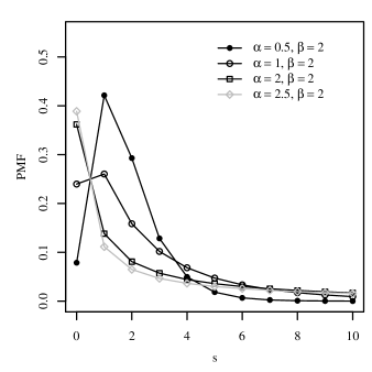
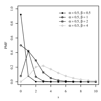
Figure 1: Plots of the PMFs for several parameter values.

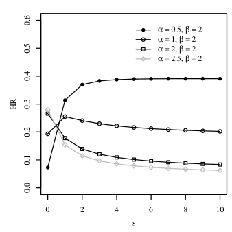
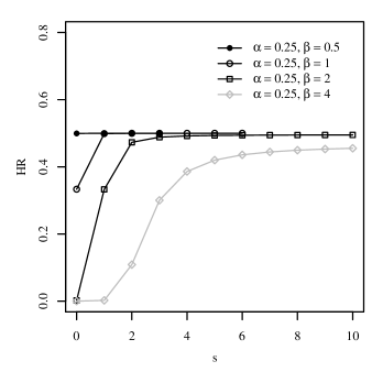
Figure 2: $\text{BS}_{\text{d}}$ HRs for some parameter values.

2.1 Properties

We present some properties of the ${\rm BS_{d}}$ distribution, many of the results can be easily derived from the definition of the ${\rm BS_{d}}$ distribution.

Proposition 1.

If $S\sim{\rm BS_{d}}(\bm{\theta})$ and $t>0$, the following holds:

• $\sum_{s=0}^{\infty}\Phi\big{[}a({s+1};\bm{\theta})\big{]}=1+\sum_{s=0}^{\infty}\Phi\big{[}a({s};\bm{\theta})\big{]};$

• $\mathbb{P}(S\leq t)=\mathbb{P}(S\leq\lfloor t\rfloor)=\Phi\big{[}a({\lfloor t\rfloor+1};\bm{\theta})\big{]}=\mathbb{P}(T\leq\lfloor t\rfloor+1);$

• $\mathbb{P}(S<t)=\mathbb{P}(T\leq\lfloor t\rfloor);$

• $\mathbb{P}(S\geq t)=\mathbb{P}(T\geq\lfloor t\rfloor+1);$

• $\mathbb{P}(S\leq\lfloor t\rfloor)=\mathbb{P}(T\leq\lfloor t\rfloor+1);$

• $\mathbb{P}(S\geq\lfloor t\rfloor)=\mathbb{P}(T>\lfloor t\rfloor)$.

2.1.1 $\boldsymbol{p}$-th quantile

Proposition 2.

Let $S\sim{\rm BS_{d}}(\bm{\theta})$ and $Q_{p}$ the quantile function in (2), $p\in(0,1)$. Then,

• If $Q_{p}>0$ is a natural number, then $Q_{p}-1$ is the $p$-th quantile of the distribution of $S$;

• If $Q_{p}>0$ is not a natural number, then $p$-th quantile of the distribution of $S$ can be represented by any value in the interval $\big{[}\lfloor Q_{p}\rfloor,\lfloor Q_{p}\rfloor+1\big{)}$.

Proof.

Since $Q_{p}$ is the $p$-th quantile for the continuous random variable $T\sim{\rm BS}(\bm{\theta})$, from Proposition 1, Item (e), we have

$$\mathbb{P}(S<Q_{p}-1)\leq\mathbb{P}(S\leq Q_{p}-1)\stackrel{{\scriptstyle\rm(e)}}{{=}}\mathbb{P}(T\leq Q_{p})=p,\quad S\sim{\rm BS_{d}}(\bm{\theta}),$$

whenever $Q_{p}>0$ is a natural number. So, we have that $Q_{p}-1$ is the $p$-th quantile of the distribution of $S$. This proves the first item.

Now, let $t=Q_{p}>0$ be not a natural number. From Items (d) and (c) of Proposition 1 and from inequalities $\lfloor Q_{p}\rfloor\leq Q_{p}\leq\lfloor Q_{p}\rfloor+1$, we have the following

$$\mathbb{P}(S<Q_{p})\stackrel{{\scriptstyle\rm(d)}}{{=}}\mathbb{P}(T\leq\lfloor Q_{p}\rfloor)\leq\mathbb{P}(T\leq Q_{p})=p,$$

$$\mathbb{P}(S\leq Q_{p})\stackrel{{\scriptstyle\rm(c)}}{{=}}\mathbb{P}(T\leq\lfloor Q_{p}\rfloor+1)\geq\mathbb{P}(T\leq Q_{p})=p,$$

and consequently $\mathbb{P}(S<Q_{p})\leq p\leq\mathbb{P}(S\leq Q_{p})$. This will be true for any $\lfloor Q_{p}\rfloor\leq t<\lfloor Q_{p}\rfloor+1$. So, we have that, at the percentage point $p$, the quantile for $S$ can be represented by any value in $\big{[}\lfloor Q_{p}\rfloor,\lfloor Q_{p}\rfloor+1\big{)}$. Thus we complete the proof. ∎

Remark 1.

If $p=0.5,$ then $Q_{p}=\beta$. If $\beta$ is a natural number, by Proposition 2-(a), $m=\beta-1$ is the median of the distribution of $S$. Already, if $\beta$ is not a natural number, by Proposition 2-(b), each $y\in\big{[}\lfloor\beta\rfloor,\lfloor\beta\rfloor+1\big{)}$ represents a median for $S$.

2.1.2 Shape properties

The next two results are related to the unimodality of the ${\rm BS_{d}}$ distribution.

Proposition 3.

The ${\rm BS_{d}}$ distribution is unimodal.

Proof.

Let $T\sim{\rm BS}(\bm{\theta})$ be a random variable with continuous ${\rm BS}$ distribution. Let $f_{T}(t;\bm{\theta})$, $t>0$ be their respective PDF. It is well-known that this distribution is unimodal (see Proposition 7 in Vila et al., (2020)), then there exists a unique point $t_{0}>0$ such that its PDF satisfies the following inequalities:

$$f_{T}(t;\bm{\theta})\geq f_{T}(t-1;\bm{\theta}),\quad\text{for all}\ t\leq t_{0},$$

and

$$f_{T}(t;\bm{\theta})\geq f_{T}(t+1;\bm{\theta}),\quad\text{for all}\ t\geq t_{0}.$$

If $s$ is a natural number such that $s\leq\lfloor t_{0}\rfloor-1$, then

$$\mathbb{P}(S=s)=\int_{s}^{s+1}f_{T}(t;\bm{\theta})\,{\rm d}t\geq\int_{s}^{s+1}f_{T}(t-1;\bm{\theta})\,{\rm d}t=\mathbb{P}(S=s-1),$$

or equivalently,

$$\mathbb{P}(S=s)-\mathbb{P}(S=s-1)\geq 0\quad\text{for all}\ s\leq\lfloor t_{0}\rfloor-1.$$

Similarly, for $s\geq\lfloor t_{0}\rfloor+1$, we obtain

$$\mathbb{P}(S=s+1)-\mathbb{P}(S=s)\leq 0.$$

It follows that $\big{\{}\mathbb{P}(S=s):s=0,1,2,\ldots\big{\}}$ is unimodal, whatever sign $\mathbb{P}(S=\lfloor t_{0}\rfloor)-\mathbb{P}(S=\lfloor t_{0}\rfloor-1)$ may have. ∎

Remark 2.

As a sub-product of the proof of Proposition 3, the mode of the ${\rm BS_{d}}$ distribution is $\lfloor t_{0}\rfloor$, where $t_{0}$ is the mode of the corresponding continuous ${\rm BS}$ distribution.

Proposition 4.

The ${\rm BS_{d}}$ distribution has a unique mode in the set $\big{\{}s=0,1,\ldots:0\leq s\leq\lfloor\beta\rfloor\big{\}}$.

Proof.

Proposition 3 guarantees the uniqueness of mode. It remains to prove that the ${\rm BS_{d}}$ distribution $\mathbb{P}(S=s)$ is decreasing for all $s\geq\lfloor\beta\rfloor+1$. We prove this by comparing the continuous BS distribution with the corresponding ${\rm BS_{d}}$ distribution. Indeed, in Lemma 2.1. of Vila et al., (2020) is proved that the PDF $f_{T}(t;\bm{\theta})$ of the continuous BS distribution is a decreasing function when $t>\beta$. However this extends to every $t\geq\beta$ because $\big{\{}{{\rm d}\over{\rm d}t}\log[f_{T}(t;\bm{\theta})]\big{\}}|_{t=\beta}=a^{\prime\prime}(\beta;\bm{\theta})/a^{\prime}(\beta;\bm{\theta})<0$. Hence, as a sub-product of the proof of Proposition 3, it follows that the ${\rm BS_{d}}$ PMF (3) is decreasing for all $s\geq\lfloor\beta\rfloor+1$. Thus, we have completed the proof. ∎

2.1.3 Order statistics

Proposition 5.

If $S_{1},\ldots,S_{n}$ is a sequence of independent and identically distributed random variables such that $S_{1}\sim{\rm BS_{d}}(\bm{\theta})$, then, the $i$th; $i=1,2,\ldots,n$; order statistic of the ${\rm BS_{d}}$ distribution, denoted $S_{(i)}$, can be written as

$$\mathbb{P}(S_{(i)}\leq s)=\sum_{k=i}^{n}\sum_{j=0}^{n-k}\binom{n}{k}\binom{n-k}{j}(-1)^{j}{F}\big{[}a({\lfloor s\rfloor};\bm{\theta});k+j\big{]},\quad s\geq 1,$$

where ${F}[\cdot;k+j]$ denotes the CDF of the power normal distribution (PND). Different properties of the PND have been discussed by Gupta and Gupta, (2008).

Proof.

It is well-known that $\mathbb{P}(S_{(i)}\leq s)=\sum_{k=i}^{n}\binom{n}{k}[F(s;\bm{\theta})]^{k}[R(s;\bm{\theta})]^{n-k}$, $s\geq 1$ (see Item (2.7) of Shahbaz et al., (2016)). Using the Newton binomial formula and the definition of a PND, the proof follows. ∎

Remark 3.

By using the identity $\sum_{k=i}^{n}\binom{n}{k}p^{k}(1-p)^{n-k}=i\binom{n}{i}\int_{0}^{p}t^{i-1}(1-t)^{n-i}\,{\rm d}t,$ the distribution function of $S_{(i)}$ can also be written as

$${P}(S_{(i)}\leq s)={\Gamma(n+1)\over\Gamma(i)\Gamma(n-i+1)}\,\int_{0}^{\Phi[a(\lfloor s\rfloor;\bm{\theta})]}t^{i-1}(1-t)^{n-i}\,{\rm d}t,\quad s\geq 1,$$

where $\Gamma(\cdot)$ is the Gamma function.

2.1.4 Mean residual life function and variance residual life function

Let $S\sim{\rm BS_{d}}(\bm{\theta})$, the mean residual life function (MRLF) and variance residual life function (VRLF) are defined by

$$\mu_{S}(k)={\mathbb{E}(S-k|S\geq k)}={\sum_{s=k}^{\infty}R(s;\bm{\theta})\over R(k-1;\bm{\theta})}$$

and

$$\sigma^{2}_{S}(k)={\rm Var}(S-k|S\geq k)=2{\sum_{s=k}^{\infty}s\,R(s;\bm{\theta})\over R(k-1;\bm{\theta})}-(2k-1)\mu_{S}(k)-\mu^{2}_{S}(k),$$

respectively, where $R(s;\bm{\theta})$ is given in (4) and $k=0,1,\ldots,$.

Proposition 6.

Let $S\sim{\rm BS_{d}}(\bm{\theta})$ with $\bm{\theta}$ belongs to the set $\Theta=\big{\{}\bm{\theta}_{*}\in(0,\infty)^{2}:\ C(t;\bm{\theta}_{*})=a^{\prime\prime}(t;\bm{\theta}_{*})-a(t;\bm{\theta}_{*})[a^{\prime}(t;\bm{\theta}_{*})]^{2}>0,\ \ \forall\ t>0\big{\}}.$ Then,

• $S$ has decreasing MRLF;

• $S$ has increasing HR;

• $S$ has decreasing VRLF,

whenever $\mathbb{P}(S>0)=1$.

Proof.

For $\bm{\theta}\in\Theta$, we have

$${{\rm d}^{2}\over{\rm d}t^{2}}\log\big{[}R(t;\bm{\theta})\big{]} =-{\phi\big{[}a(t;\bm{\theta})\big{]}\over 1-\Phi\big{[}a(t;\bm{\theta})\big{]}}\,\left\{{\phi\big{[}a(t;\bm{\theta})\big{]}\big{[}a^{\prime}(t;\bm{\theta})\big{]}^{2}\over 1-\Phi\big{[}a(t;\bm{\theta})\big{]}}+C(t;\bm{\theta})\right\}<0\quad\text{for all}\ t>0.$$

In other words, the function $\log[R(t;\bm{\theta})]$ is concave. This condition implies that $\log\big{[}R({t_{1}+t_{2}\over 2};\bm{\theta})\big{]}\geq{1\over 2}\log\big{[}R(t_{1};\bm{\theta})\big{]}+{1\over 2}\log\big{[}R(t_{2};\bm{\theta})\big{]}$ or equivalently that $\big{[}R({t_{1}+t_{2}\over 2};\bm{\theta})\big{]}^{2}\geq R(t_{1};\bm{\theta})R(t_{2};\bm{\theta})$ for all $t_{1},t_{2}>0.$ Hence, taking $t_{1}=s+2$ and $t_{2}=s$ for $s=1,2,3,\ldots$, we have

$$\big{[}R(s+1;\bm{\theta})\big{]}^{2}\geq R(s+2;\bm{\theta})R(s;\bm{\theta})\quad\Longleftrightarrow\quad H(s+1;\bm{\theta})\leqslant H(s+2;\bm{\theta}).$$

That is, $S$ has increasing hazard rate $H(\cdot;\bm{\theta})$. Then, by Theorem 2.1 of Gupta, (2015), it follows that $S$ has decreasing mean residual life function. This proves the statement in Items (a) and (b). Finally, the proof of Item (c) follows directly by combining Item (a) with Theorem 2.2 in Gupta, (2015). ∎

2.1.5 Moments properties

Proposition 7.

The distribution of a random variable $S$ with ${\rm BS_{d}}$ distribution has all moments.

Proof.

In Proposition 3 is proved that $S$ has a strongly unimodal distribution (see Keilson and Gerber, (1971), for a formal definition). Since that all strongly unimodal distribution have all moments (see Theorem 7 in Keilson and Gerber, (1971)), the proof of the proposition follows. ∎

Proposition 8.

If $S\sim{\rm BS_{d}}(\bm{\theta})$ is a random variable, for each natural number $r$, we have

$$\begin{array}[]{lllll}\textrm{\rm(a)}&\displaystyle\mathbb{E}(S^{r})=\sum_{s=0}^{\infty}\big{[}(s+1)^{r}-s^{r}\big{]}\left\{1-\Phi\big{[}a(s+1;\bm{\theta})\big{]}\right\};\\[14.22636pt] \textrm{\rm(b)}&\displaystyle\mathbb{E}(S^{r})=\sum_{s=0}^{\infty}\sum_{k=0}^{r}\sum_{i=0}^{r-k}\binom{r-k}{i}s^{k+i}\,\left\{1-\Phi\big{[}a(s+1;\bm{\theta})\big{]}\right\};\\[18.49411pt] \textrm{\rm(c)}&\displaystyle{\rm Var}(S)=2\sum_{s=0}^{\infty}s\left\{1-\Phi\big{[}a(s+1;\bm{\theta})\big{]}\right\}\\[5.69046pt] &\qquad\quad\,+\displaystyle\sum_{s=0}^{\infty}\left\{1-\Phi\big{[}a(s+1;\bm{\theta})\big{]}\right\}\bigg{[}1-\sum_{s=0}^{\infty}\left\{1-\Phi\big{[}a(s+1;\bm{\theta})\big{]}\right\}\bigg{]}.\end{array}$$

Proof.

The whole proof follows closely Proposition 2 of Saulo et al., (2021) and we present it for the sake of completeness. We emphasize that the statements of Items (a), (b) and (c) are valid for any discrete random variable $S$ with support $\{0,1,\ldots\}$.

By using the telescopic series $\sum_{x=0}^{i-1}[(x+1)^{r}-x^{r}]=i^{r}$, we have

$$\mathbb{E}(S^{r}) =\sum_{i=0}^{\infty}\sum_{s=0}^{\infty}\mathds{1}_{\{s<i\}}[(s+1)^{r}-s^{r}]\,\mathbb{P}(S=i)$$

$$=\sum_{s=0}^{\infty}[(s+1)^{r}-s^{r}]\sum_{i=0}^{\infty}\mathds{1}_{\{i>s\}}\,\mathbb{P}(S=i),$$

where in the second equality we exchange the orders of the summations because

$$\sum_{s=0}^{\infty}\mathds{1}_{\{s<i\}}\big{|}(s+1)^{r}-s^{r}\big{|}\,\mathbb{P}(S=i)=\sum_{s=0}^{\infty}\mathds{1}_{\{s<i\}}\cdot[(s+1)^{r}-s^{r}]\,\mathbb{P}(S=i)=i^{r}\mathbb{P}(S=i),$$

is finite for each $i=0,1,\ldots$; and because $\sum_{i=0}^{\infty}i^{r}\mathbb{P}(S=i)=\mathbb{E}(S^{r})$ always exists (see Proposition 7). This proves Item (a). The second item follows by combining Item (a) with the polynomial identity $a^{n}-b^{n}=(a-b)\sum_{k=0}^{r}a^{r-k}b^{k}$ and the binomial expansion. Already, the proof of Item (c) is obtained by using Item (a) and simple algebraic manipulations. ∎

2.2 Maximum likelihood estimation

In this section, we discuss the maximum likelihood estimation for the unknown model parameters based on a random sample $S_{1},S_{2},\ldots,S_{n}$ from $S\sim{\rm BS_{d}}(\bm{\theta})$, with $\bm{\theta}=(\alpha,\beta)$. Thus, the log-likelihood function for $\bm{\theta}$ is given by

$$l(\bm{\theta})=\sum_{i=1}^{n}\log\left\{\Phi\big{[}a({s_{i}+1};\bm{\theta})\big{]}-\Phi\big{[}a({s_{i}};\bm{\theta})\big{]}\right\}.$$ (6)

In order to obtain the maximum likelihood estimate of $\bm{\theta}$, we have the score function given by $\dot{\bm{l}}(\bm{\theta})=[\dot{l}_{\alpha}(\bm{\theta}),\dot{l}_{\beta}(\bm{\theta})]^{\top}$, whose elements are given by

$$\dot{l}_{z}(\bm{\theta}) =\sum_{i=1}^{n}\sum_{j=0}^{1}(-1)^{j+1}\,{\partial a({s_{i}+j};\bm{\theta})\over\partial z}\,\phi_{j}(s_{i},\bm{\theta}),\quad z\in\{\alpha,\beta\},$$ (7)

where

$$\frac{\partial a(s_{i};\bm{\theta})}{\partial\alpha} = -\frac{1}{\alpha}a(s_{i};\bm{\theta}),\,\frac{\partial a(s;\bm{\theta})}{\partial\beta}=-\frac{1}{2\alpha}\frac{1}{s^{1/2}\beta^{3/2}}(s+\beta)\,\,{\rm and}\,\phi_{j}(s_{i},\bm{\theta})={\phi\big{[}a({s_{i}+j};\bm{\theta})\big{]}\over\mathbb{P}(S=s_{i})}.$$

The maximum likelihood estimate of $\alpha$ and $\beta$ can be obtained solving the equations $\dot{l}_{\alpha}(\bm{\theta})=0$ and $\dot{l}_{\beta}(\bm{\theta})=0$ by an iterative procedure for non-linear optimization. The Hessian matrix of ${l}(\bm{\theta})$ is given by $\ddot{\bm{l}}(\bm{\theta})=\big{[}\frac{\partial^{2}l(\bm{\theta})}{\partial z\partial w}\big{]}_{2\times 2},$ for each $w,z\in\{\alpha,\beta\}$, where

$$\ddot{l}_{wz}(\bm{\theta}) = \sum_{i=1}^{n}\sum_{j=0}^{1}(-1)^{j+1}{\partial^{2}a({s_{i}+j};\bm{\theta})\over\partial w\partial z}\,{\phi_{j}(s_{i},\bm{\theta})}$$ (8)

$$- \sum_{i=1}^{n}\sum_{j=0}^{1}(-1)^{j+1}a({s_{i}+j};\bm{\theta})\,{\partial a({s_{i}+j};\bm{\theta})\over\partial w}\,{\partial a({s_{i}+j};\bm{\theta})\over\partial z}\,{\phi_{j}(s_{i},\bm{\theta})}$$

$$- \sum_{i=1}^{n}\sum_{j=0}^{1}(-1)^{j+1}{\partial a({s_{i}+j};\bm{\theta})\over\partial z}\,{\phi_{j}\big{[}s_{i},\bm{\theta}\big{]}}\sum_{k=0}^{1}(-1)^{k+1}\,{\partial a({s_{i}+k};\bm{\theta})\over\partial w}\,{\phi_{k}(s_{i},\bm{\theta})},$$

where $\phi_{j}(s_{i},\bm{\theta})$ is as in (7) and the second-order partial derivatives of $a(\cdot;\bm{\theta})$, with respect to the parameters, are given by

$$\frac{\partial^{2}a(s_{i};\bm{\theta})}{\partial\alpha\partial\alpha} = \frac{2}{\alpha^{2}}a(s_{i}),\,\,\,\frac{\partial^{2}a(s_{i};\bm{\theta})}{\partial\beta\partial\alpha}=-\frac{1}{\alpha}\frac{\partial a(s_{i};\bm{\theta})}{\partial\beta},\,\,\,\frac{\partial^{2}a(s_{i};\bm{\theta})}{\partial\beta\partial\beta}=\frac{1}{4\alpha s_{i}^{1/2}\beta^{5/2}}(3s_{i}+\beta).$$

3 Discrete Birnbaum-Saunders regression model

In the context of count data, the ${\rm BS_{d}}$ distribution may be an interesting alternative distribution to usual discrete distributions or to those discrete distributions have been derived from continuous distributions. Then, for the ${\rm BS_{d}}$ distribution we are also going to consider its associated regression model, which will be the goal of this part of the study. The associated ${\rm BS_{d}}$ regression model that we are going to introduce is inspired by continuous BS regression model developed by Balakrishnan and Zhu, (2015), where they considered the scale parameter depending on covariates.

Suppose that we observe independent failure times $S_{1},\ldots,S_{n}$, such as

$$S_{i}\sim{\rm BS_{d}}(\bm{\theta}_{i}),$$ (9)

where $\bm{\theta}_{i}=(\alpha,\beta_{i})$, $i=1,\ldots,n$. The distribution depends on covariates $\bm{x}_{i}=(x_{1i},\ldots,x_{pi})^{\top}$ associated with $\beta_{i}$ thought $\beta_{i}=\exp(\bm{x}_{i}^{\top}\bm{\eta})$, with $\bm{\eta}=(\eta_{0},\eta_{1},\ldots,\eta_{p})^{\top}$ being a vector of unknown parameters. The corresponding PMF associated with (9) is

$$\mathbb{P}(S_{i}=s_{i}) = \Phi\big{[}a(s_{i};\bm{\theta}_{i})\big{]}\mathds{1}_{\{s_{i}=0\}}+\left\{\Phi\left(a(s_{i}+1;\bm{\theta}_{i})\right)-\Phi\left(a(s_{i};\bm{\theta}_{i})\right)\right\}\mathds{1}_{\{s_{i}\geqslant 1\}},$$

$i=1,\ldots,n$.

3.1 Maximum likelihood estimation

The log-likelihood function for ${\bm{\theta}}=(\alpha,\bm{\eta}^{\top})^{\top}$ is given by

$$l(\bm{\theta}) = \sum_{i=1}^{n}\log\left\{\Phi\big{[}a(s_{i};\bm{\theta}_{i})\big{]}\mathds{1}_{\{s_{i}=0\}}+\left\{\Phi\left(a(s_{i}+1;\bm{\theta}_{i})\right)-\Phi\left(a(s_{i};\bm{\theta}_{i})\right)\right\}\mathds{1}_{\{s_{i}\geqslant 1\}}\right\}.$$ (10)

Then, the first derivatives of the log-likelihood function (10), with ${\bm{\theta}}=(\alpha,\bm{\eta}^{\top})^{\top}$, can be written as

$$\dot{l}_{u}(\bm{\theta}) = \sum_{i=1}^{n}\sum_{j=0}^{1}(-1)^{j+1}\,{\partial a({s_{i}+j};\bm{\theta})\over\partial z_{i}}\,{\partial z_{i}\over\partial u}\,\phi_{j}(s_{i},\bm{\theta})\quad u\in\{\alpha,\bm{\eta}\},z_{i}\in\{\alpha,\beta_{i}\},$$

where $\dot{l}_{u}(\bm{\theta})={\partial l(\bm{\theta})}/{\partial u}$, and ${\partial a({s}_{i};\bm{\theta})/\partial z_{i}}$ is as in (7). Specifically

$$\dot{l}_{\alpha}(\bm{\theta}) = \sum_{i=1}^{n}\sum_{j=0}^{1}(-1)^{j+1}\,{\partial a({s_{i}+j};\bm{\theta})\over\partial\alpha}\,\phi_{j}(s_{i},\bm{\theta}),$$

$$\dot{l}_{\eta}(\bm{\theta}) = \sum_{i=1}^{n}\sum_{j=0}^{1}(-1)^{j+1}\,{\partial a({s_{i}+j};\bm{\theta})\over\partial\beta_{i}}\,\phi_{j}(s_{i},\bm{\theta}){\partial\beta_{i}\over\partial\bm{\eta}},$$

where ${\partial\beta_{i}/\partial\bm{\eta}}=\beta_{i}\bm{x}_{i};i=1,\ldots,n.$ From the likelihood equations $\dot{l}_{\alpha}(\bm{\theta})=0$ and $\dot{l}_{\eta}(\bm{\theta})=0$, we can see that there is no closed-form solution to the maximization problem, so we implement two algorithms in software R to find the maximum likelihood estimates of $\alpha$, $\beta$ and $\eta_{i}$, $i=0,\ldots,p$, by using the function optim(); see R Core Team, (2020). These procedures are evaluated and used in the next section.

Furthermore, the Hessian matrix of $l(\bm{\theta})$ is given by

$$\big{[}\ddot{l}_{vu}(\bm{\theta})\big{]}_{p\times p}=\begin{bmatrix}\frac{\partial^{2}l(\bm{\theta})}{\partial\alpha^{2}}&\frac{\partial^{2}l(\bm{\theta})}{\partial\alpha\partial\bm{\eta}^{\top}}\\[5.69046pt] \frac{\partial^{2}l(\bm{\theta})}{\partial\bm{\eta}\partial\alpha}&\frac{\partial^{2}l(\bm{\theta})}{\partial\bm{\eta}\partial\bm{\eta}^{\top}}\end{bmatrix},$$

where, for each $v,u\in\{\alpha,\bm{\eta}\}$ and $w_{i},z_{i}\in\{\alpha,\beta_{i}\}$, the elements of the Hessian matrix are given by

$$\ddot{l}_{vu}(\bm{\theta}) = \sum_{i=1}^{n}\sum_{j=0}^{1}(-1)^{j+1}\left[{\partial^{2}a({s_{i}+j};\bm{\theta})\over\partial w_{i}\partial z_{i}}\,{\partial z_{i}\over\partial u}\,{\partial w_{i}\over\partial v}+{\partial a({s_{i}+j};\bm{\theta})\over\partial z_{i}}\,{\partial^{2}z_{i}\over\partial v\partial u}\right]\phi_{j}(s_{i},\bm{\theta})$$

$$- \sum_{i=1}^{n}\sum_{j=0}^{1}(-1)^{j+1}a({s_{i}+j};\bm{\theta})\,{\partial a({s_{i}+j};\bm{\theta})\over\partial w_{i}}\,{\partial a({s_{i}+j};\bm{\theta})\over\partial z_{i}}\,{\partial z_{i}\over\partial u}\,{\partial w_{i}\over\partial v}\,\phi_{j}(s_{i},\bm{\theta})$$

$$- \sum_{i=1}^{n}\sum_{j=0}^{1}(-1)^{j+1}{\partial a({s_{i}+j};\bm{\theta})\over\partial z_{i}}\,\phi_{j}(s_{i},\bm{\theta})\sum_{k=0}^{1}(-1)^{k+1}\,{\partial a({s_{i}+k};\bm{\theta})\over\partial w_{i}}\,{\partial z_{i}\over\partial u}\,{\partial w_{i}\over\partial v}\,\phi_{k}(s_{i},\bm{\theta}),$$

where ${\partial^{2}a({s}_{i};\bm{\theta})/\partial w_{i}\partial z_{i}}$ is as in (8) and

$$\frac{\partial\beta_{i}}{\partial\bm{\eta}}=\beta_{i}\bm{x}_{i}\,\,\,{\rm and}\,\,\,\frac{\partial^{2}\beta_{i}}{\partial\bm{\eta}\partial\bm{\eta}^{\top}}=\beta_{i}\bm{x}_{i}\bm{x}_{i}^{\top}$$

Again, note that the equation $\dot{l}_{u}(\bm{\theta})=\bm{0}$ does not provides analytic solutions for $\widehat{\alpha}$ and $\widehat{\eta_{j}}$, $j=0,\ldots,p$. Therefore, we have implemented two algorithms in software R to find the maximum likelihood estimates of $\alpha$ and $\eta_{i}$, $i=0,\ldots,p$, by using the function optim(); see R Core Team, (2020). These procedures are evaluated and used in the next section.

4 Numerical evaluation

In this section we carry out a simulation study to evaluate the performance of both the maximum likelihood estimators and residuals. Moreover, we analyse two real data sets. All numerical evaluations were done in the R software; see R Core Team, (2019). The R codes are available upon request from the authors.

4.1 Simulation

We first evaluate the performance of the maximum likelihood estimators for the $S\sim{\rm BS_{d}}$ model. Then, we consider a ${\rm BS_{d}}$ regression model where the parameter $\beta$ is associated with a covariate, that is,

$$\beta_{i}=\exp(\eta_{0}+\eta_{1}x_{i})\quad i=1,\ldots,n.$$ (11)

In (11), the covariate values were randomly generated from the uniform distribution in the interval (0,1). The simulation scenario considers: sample size $n\in\{10,50,150,400\}$ and the values of the shape parameter as $\alpha\in\{0.50,1.50,1.50,3.00\}$ , with $1,000$ Monte Carlo replications for each sample size. The values of $\alpha$ have been chosen to cover the performance under low, moderate and high skewness. The $\text{BS}_{\text{d}}$ samples were generated using the Proposition 2.

The maximum likelihood estimation results for the ${\rm BS_{d}}$ model are presented in Table 1. We report the following sample statistics for the maximum likelihood estimates: empirical bias and mean squared error (MSE). Note that the results in Table 1 allows us to conclude that, as the sample size increases, the bias and MSE of the estimators $\widehat{\alpha}$ and $\widehat{\beta}$ decrease, indicating that they are asymptotically unbiased, as expected.

Table 1: Simulated values of biases (MSEs within parentheses) of the estimators of the ${\rm BS_{d}}$ model ($\beta=2$).

		$n=10$			$n=50$
		$\widehat{\alpha}$	$\widehat{\beta}$		$\widehat{\alpha}$	$\widehat{\beta}$
0.5		$-$0.0406(0.0213)	0.0281(0.1052)		$-$0.0075(0.0035)	0.0038(0.0199)
1.5		$-$0.1462(0.1710)	0.1138(0.7972)		0.0047(0.0488)	0.0207(0.1785)
2.5		$-$0.4642(0.6149)	0.8073(2.6281)		$-$0.1262(0.1424)	0.2500(0.3770)
3.0		$-$0.6597(0.9420)	1.2008(4.5642)		$-$0.2351(0.2279)	0.4059(0.5581)
		$n=150$			$n=400$
0.5		$-$0.0013(0.0011)	0.0017(0.0069)		$-$0.0002(0.0004)	$-$0.0013(0.0026)
1.5		$-$0.0021(0.0157)	$-$0.0018(0.0566)		$-$0.0007(0.0062)	$-$0.0028(0.0215)
2.5		$-$0.0372(0.0531)	0.1024(0.1312)		$-$0.0135(0.0255)	0.0319(0.0561)
3.0		$-$0.0998(0.0918)	0.1807(0.1908)		$-$0.0180(0.0433)	0.0410(0.0765)

Table 2 reports the simulation results for the ${\rm BS_{d}}$ regression model. A look at the results in Table 2 allows us to conclude that, as the sample size increases, the empirical bias and MSE decrease, as expected. Moreover, we note that, as the value of the parameter $\alpha$ increases, the performances of the estimators of $\beta_{0}$, $\beta_{1}$ and $\alpha$, deteriorate.

Table 2: Simulated values of biases (MSEs within parentheses) of the estimators of the ${\rm BS_{d}}$ regression model ($\eta_{0}=0.2$ and $\eta_{0}=1.5$).

		$n=10$				$n=50$
		$\widehat{\eta}_{0}$	$\widehat{\eta}_{1}$	$\widehat{\alpha}$		$\widehat{\eta}_{0}$	$\widehat{\eta}_{1}$	$\widehat{\alpha}$
0.5		0.0122(0.1581)	$-$0.0065(0.4129)	$-$0.0586(0.0155)		0.0046(0.0235)	$-$0.0043(0.0665)	$-$0.0104(0.0027)
1.5		$-$0.0457(1.1930)	0.0621(3.0408)	$-$0.1665(0.1672)		$-$0.0072(0.1611)	0.0108(0.4365)	$-$0.0268(0.0279)
2.5		$-$0.2260(3.6180)	0.1322(8.2195)	$-$0.0438(3.0714)		$-$0.0473(0.3325)	0.0326(0.8433)	$-$0.0119(0.1108)
3.0		$-$0.3103(5.2066)	0.1576(11.5868)	0.2436(23.5472)		$-$0.0632(0.4081)	0.0242(0.9987)	0.0156(0.2055)
		$n=150$				$n=400$
0.5		$-$0.0003(0.0082)	0.0023(0.0212)	$-$0.0027(0.0009)		$-$0.0007(0.0030)	0.0011(0.0078)	$-$0.0009(0.0004)
1.5		$-$0.0087(0.0534)	0.0160(0.1354)	$-$0.0072(0.0092)		$-$0.0043(0.0190)	0.0039(0.0499)	$-$0.0015(0.0036)
2.5		$-$0.0195(0.1057)	0.0208(0.2493)	$-$0.0034(0.0359)		$-$0.0128(0.0356)	0.0107(0.0879)	0.0024(0.0133)
3.0		$-$0.0270(0.1289)	0.0209(0.2983)	0.0063(0.0590)		$-$0.0166(0.0433)	0.0143(0.1003)	0.0050(0.0230)

4.2 Examples

The ${\rm BS_{d}}$ distribution and its regression model proposed in Section 3 are now used to analyze two data sets. In the first case, the objective is to fit the BS_d distribution to data corresponding to biaxial fatigue-life of $n=46$ metal specimens (in cycles) until failure; this data set can be found in Rieck, J., (1989). In the second example, we fit the proposed regression model to data on the fatigue-life (in cycles $\times 10^{-3}$) of concrete specimens (response variable $Y$), where the covariate is the ratio of applied stress causing failure (covariate $x$); see Mills, J., (1997). In this second data set, the number of observations is $n=45$.

Case study 1: Metal specimens

A descriptive summary of this data provides the following sample values: 566(median); 943.065(mean); 1110.934(standard deviation); 117.8(coefficient of variation); 2.204(coefficient of skewness); 4.682(coefficient of kurtosis), whereas their minimum and maximum times are 125 and 5046, respectively. The histogram shown in Figure 3 and the value of the coefficient of skewness support the assumption that these data follow an asymmetrical distribution. We have assumed different discrete asymmetrical distributions to describe this data set, including the Weibull, gamma, log-normal, log-Student-$t$, and log-power-exponential (log-PE) distributions; see Nakagawa and Osaki, (1975), Abouammoh and Alhazzani, (2015), and Saulo et al., (2021). Table 3 presents the Akaike (AIC) and Bayesian (BIC) information criteria. The results of Table 3 reveal that the BS_d model provides better adjustment than the other models based on the values of AIC and BIC. The estimates and standard errors (in parenthesis) for the BS_d model are $\widehat{\alpha}=1.0840(0.1130)$ and $\widehat{\beta}=595.1987(81.6782)$, and the fitted PMF is also shown in Figure 3.

Table 3: Values of AIC and BIC for different discrete asymmetrical distributions.

criterion	Weibull	Gamma	log-normal	log-Student-$t$	log-PE	BSd
AIC	726.1691	726.1692	718.8391	719.7321	715.8479	714.8548
BIC	729.8264	729.8265	724.3250	725.2181	721.3338	718.5121

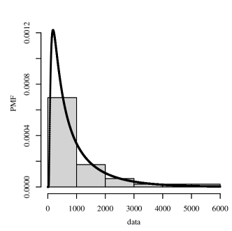
Figure 3: histogram for data of metal specimens.

Case study 2: Concrete specimens

The number of cycles until failure is expected to increase inversely with the ratio of applied stress causing failure. The postulated model is given by

$$\beta_{i}=\exp(\eta_{0}+\eta_{1}x),\quad Y_{i}\sim\textrm{BS}_{d}(\alpha,\beta_{i}),$$

for $i=1,\ldots,45$. The maximum likelihood estimates and standard errors (in parenthesis) for $\alpha$, $\eta_{0}$ and $\eta_{1}$ are $\widehat{\alpha}=0.4966(0.0641)$, $\widehat{\eta}_{0}=27.4913(3.2530)$ and $\widehat{\eta}_{1}=-23.9647(3.5146)$, respectively. Figure 4 presents the QQ plots with envelope of the generalized Cox-Snell and randomized quantile residuals for the ${\rm BS_{d}}$ regression model; see Saulo et al., (2019). Note that all points are inside the bands and around the $y=x$ line, demonstrating a very good fit of the proposed model.

(a)

(b)

Figure 4: QQ plots with envelope for the generalized Cox-Snell (a) and randomized quantile (b) residuals for the concrete specimens data.

5 Concluding remarks

The continuous Birnbaum-Saunders distribution has been widely used in several areas, besides being an alternative to the Weibull and gamma distributions. However, in many practical problems, the use of discrete distributions is more appropriate. In this sense, we have studied a discrete version of the Birnbaum-Saunders distribution. Some important properties have been presented, such as moments, quantile function and reliability. We have presented a formal proof concerning the unimodality property of discrete Birnbaum-Saunders distribution. In addition, we have proposed a new discrete Birnbaum-Saunders regression model. Monte Carlo simulations have been carried out to evaluate the behaviour of the maximum likelihood estimators. Two examples with real data have illustrated the proposed methodology. The results are seen to be quite favorable to the discrete Birnbaum-Saunders distribution as well as its regression model in terms of model fitting.

References

• Abouammoh and Alhazzani, (2015) Abouammoh, A. M. and Alhazzani, N. S. (2015). On discrete gamma distribution. Communications in Statistics - Theory and Methods, 44:3087–3098.
• Ahmed et al., (2010) Ahmed, S., Castro-Kuriss, C., Leiva, V., Flores, E., and Sanhueza, A. (2010). Truncated version of the Birnbaum-Saunders distribution with an application in financial risk. Pakistan Journal of Statistics, 26:293–311.
• Alzaatreh et al., (2012) Alzaatreh, A., Lee, C., and Famoye, F. (2012). On the discrete analogues of continuous distributions. Statistical Methodology, 9:589–603.
• Balakrishnan and Kundu, (2019) Balakrishnan, N. and Kundu, D. (2019). Birnbaum-saunders distribution: A review of models, analysis, and applications. Applied Stochastic Models in Business and Industry, 35(1):4–49.
• Balakrishnan et al., (2009) Balakrishnan, N., Leiva, V., Sanhueza, A., and Cabrera, E. (2009). Mixture inverse Gaussian distribution and its transformations, moments and applications. Statistics, 43:91–104.
• Balakrishnan and Zhu, (2015) Balakrishnan, N. and Zhu, X. (2015). Inference for the Birnbaum-Saunders lifetime regression model with applications. Communications in Statistics - Simulation and Computation, 44(8):2073–2100.
• Birnbaum and Saunders, (1969) Birnbaum, Z. W. and Saunders, S. C. (1969). A new family of life distributions. Journal of Applied Probability, 6:319–327.
• Desousa et al., (2018) Desousa, M. F., Saulo, H., Leiva, V., and Scalco, P. (2018). On a tobit-Birnbaum-Saunders model with an application to antibody response to vaccine. Journal of Applied Statistics, 45:932–955.
• Gupta, (2015) Gupta, P. L. (2015). Properties of reliability functions of discrete distributions. Communications in Statistics - Theory and Methods, 44(19):4114–4131.
• Gupta and Gupta, (2008) Gupta, R. D. and Gupta, R. C. (2008). Analyzing skewed data by power normal model. TEST, 17(1):197–210.
• Keilson and Gerber, (1971) Keilson, J. and Gerber, H. (1971). Some results for discrete unimodality. Journal of the American Statistical Association, 66(334):386–389.
• Leão et al., (2018) Leão, J., Leiva, V., Saulo, H., and Tomazella, V. (2018). Incorporation of frailties into a cure rate regression model and its diagnostics and application to melanoma data. Statistics in Medicine, 37:4421–4440.
• Leiva, (2016) Leiva, V. (2016). The Birnbaum-Saunders Distribution. Academic Press, New York, US.
• Leiva et al., (2017) Leiva, V., Ruggeri, F., Saulo, H., and Vivanco, J. F. (2017). A methodology based on the Birnbaum-Saunders distribution for reliability analysis applied to nano-materials. Reliability Engineering and System Safety, 157:192–201.
• (15) Leiva, V., Santos-Neto, M., Cysneiros, F. J. A., and Barros, M. (2014a). Birnbaum-Saunders statistical modelling: A new approach. Statistical Modelling, 14:21–48.
• (16) Leiva, V., Saulo, H., Leão, J., and Marchant, C. (2014b). A family of autoregressive conditional duration models applied to financial data. Computational Statistics and Data Analysis, 79:175–191.
• Leiva et al., (2011) Leiva, V., Soto, G., Cabrera, E., and Cabrera, G. (2011). New control charts based on the Birnbaum-Saunders distribution and their implementation. Revista Colombiana de Estadística, 34:147–176.
• Lio and Park, (2008) Lio, Y. L. and Park, C. (2008). A bootstrap control chart for Birnbaum-Saunders percentiles. Quality and Reliability Engineering International, 24:585–600.
• Marchant et al., (2013) Marchant, C., Bertin, K., Leiva, V., and Saulo, H. (2013). Generalized Birnbaum-Saunders kernel density estimators and an analysis of financial data. Computational Statistics and Data Analysis, 63:1–15.
• Mills, J., (1997) Mills, J. (1997). Robust estimation of the Birnbaum–Saunders distribution. Master thesis. Technical University of Nova Scotia, Nova Scotia, Canada.
• Nakagawa and Osaki, (1975) Nakagawa, T. and Osaki, S. (1975). The discrete weibull distributions. IEEE Trans. Reliab, 24:300–301.
• Paula et al., (2012) Paula, G. A., Leiva, V., Barros, M., and Liu, S. (2012). Robust statistical modeling using the Birnbaum-Saunders-t distribution applied to insurance. Applied Stochastic Models in Business and Industry, 28:16–34.
• R Core Team, (2019) R Core Team (2019). R: A Language and Environment for Statistical Computing. R Foundation for Statistical Computing, Vienna, Austria.
• R Core Team, (2020) R Core Team (2020). R: A language and environment for statistical computing. R Foundation for Statistical Computing, Vienna, Austria.
• Rieck, J., (1989) Rieck, J. (1989). Statistical Analysis for the Birnbaum–Saunders Fatigue Life Distribution. Ph.D. thesis. Department of Mathematical Sciences, Clemson University, Clemson.
• Rojas et al., (2015) Rojas, F., Leiva, V., Wanke, P., and Marchant, C. (2015). Optimization of contribution margins in food services by modeling independent component demand. Revista Colombiana de Estadística, 38:1–30.
• Saulo et al., (2019) Saulo, H., Leão, J., Leiva, V., and Aykroyd, R. (2019). Birnbaum-Saunders autoregressive conditional duration models applied to high-frequency financial data. Statistical Papers, 60:1605–1629.
• Saulo et al., (2021) Saulo, H., Vila, R., Paiva, L., Balakrishnan, N., and Bourguignon, M. (2021). On a family of discrete log-symmetric distributions. Journal of Statistical Theory and Practice, 15:67.
• Sen et al., (2010) Sen, S., Maiti, S., and Dey, M. (2010). Discrete birnbaum-saunders distribution and its properties related to reliability analysis. IAPQR-Transactions, 35:67–78.
• Shahbaz et al., (2016) Shahbaz, M., Ahsanullah, M., Shahbaz, S., and Al-Zahrani, B. (2016). Ordered Random Variables: Theory and Applications. Atlantis Studies in Probability and Statistics. Atlantis Press.
• Ventura et al., (2019) Ventura, M., Saulo, H., Leiva, V., and Monsueto, S. E. (2019). Log-symmetric regression models: information criteria and application to movie business and industry data. Applied Stochastic Models in Business and Industry, page DOI:10.1002/asmb.2433.
• Vila et al., (2020) Vila, R., Leão, J., Saulo, H., Shahzad, M. N., and Santos-Neto, M. (2020). On a bimodal Birnbaum-Saunders distribution with applications to lifetime data. Brazilian Journal of Probability and Statistics, 34(3):495 – 518.
• Vila et al., (2019) Vila, R., Nakano, E. Y., and Saulo, H. (2019). Theoretical results on the discrete weibull distribution of nakagawa and osaki. Statistics, 53(2):339–363.
• Vilca et al., (2010) Vilca, F., Sanhueza, A., Leiva, V., and Christakos, G. (2010). An extended Birnbaum-Saunders model and its application in the study of environmental quality in Santiago, Chile. Stochastic Environmental Research and Risk Assessment, 24:771–782.
• Wanke and Leiva, (2015) Wanke, P. and Leiva, V. (2015). Exploring the potential use of the Birnbaum-Saunders distribution in inventory management. Mathematical Problems in Engineering, Article ID 827246:1–9.